Embed Size (px)
DESCRIPTION
Get started learning Excel with this introductory step-by-step instruction.
Citation preview
For use with MS Excel 98, 2000, 2001, XP
Modified SPLC Document for use at Neighborhood House Rev 1.1.2010
Microsoft Excel: Exercise 1
Entering Information
In this exercise:
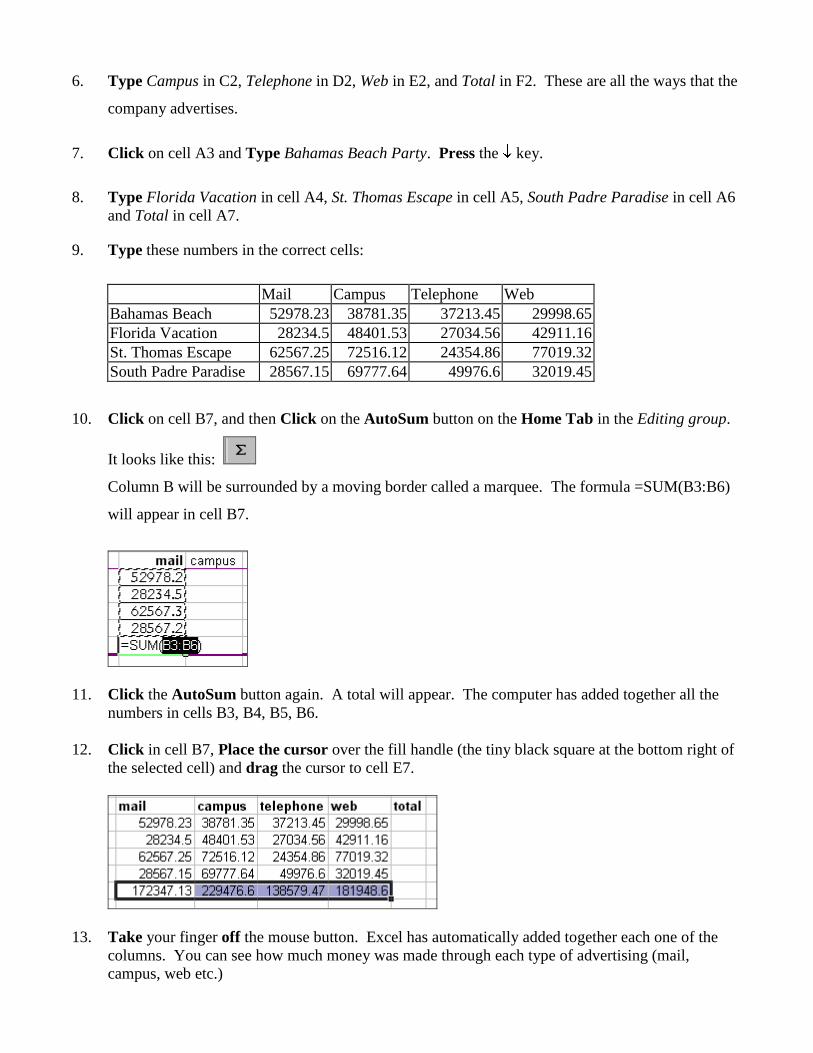
Understanding rows and columns
Typing and editing text in a cell
Formatting text in a cell
Using the series fill handle
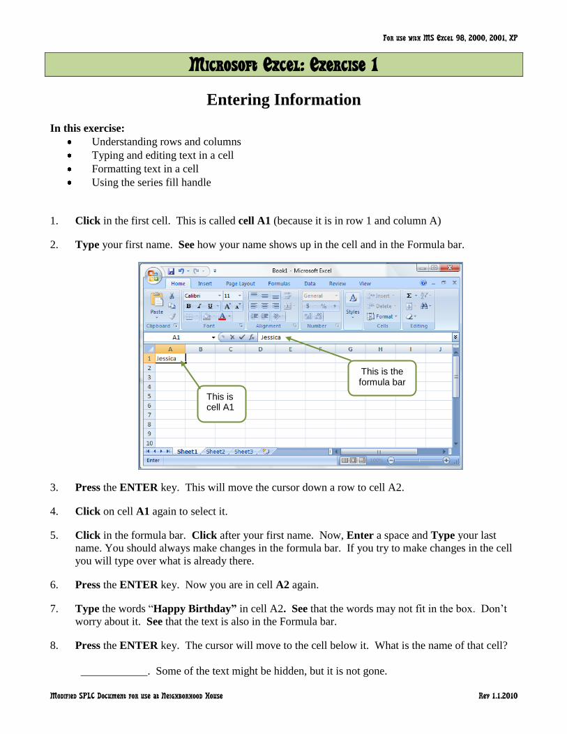
1. Click in the first cell. This is called cell A1 (because it is in row 1 and column A)
2. Type your first name. See how your name shows up in the cell and in the Formula bar.
3. Press the ENTER key. This will move the cursor down a row to cell A2.
4. Click on cell A1 again to select it.
5. Click in the formula bar. Click after your first name. Now, Enter a space and Type your last
name. You should always make changes in the formula bar. If you try to make changes in the cell
you will type over what is already there.
6. Press the ENTER key. Now you are in cell A2 again.
7. Type the words ―Happy Birthday” in cell A2. See that the words may not fit in the box. Don’t
worry about it. See that the text is also in the Formula bar.
8. Press the ENTER key. The cursor will move to the cell below it. What is the name of that cell?
____________. Some of the text might be hidden, but it is not gone.
This is the formula bar
This is cell A1
9. Click in cell A2 again, your text will return. Check the formula bar to be sure.
10. Now, click in cell B2.
11. Type the words ―dear Andrew”. Press the ENTER key.
12. Click in cell B2. Click in the formula bar and change Andrew to ―Andrea”.
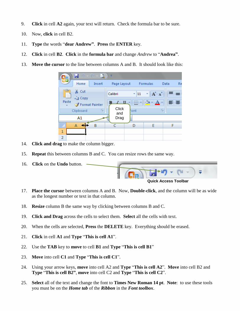
13. Move the cursor to the line between columns A and B. It should look like this:
14. Click and drag to make the column bigger.
15. Repeat this between columns B and C. You can resize rows the same way.
16. Click on the Undo button.
Quick Access Toolbar
17. Place the cursor between columns A and B. Now, Double-click, and the column will be as wide
as the longest number or text in that column.
18. Resize column B the same way by clicking between columns B and C.
19. Click and Drag across the cells to select them. Select all the cells with text.
20. When the cells are selected, Press the DELETE key. Everything should be erased.
21. Click in cell A1 and Type ―This is cell A1‖.
22. Use the TAB key to move to cell B1 and Type ―This is cell B1‖
23. Move into cell C1 and Type ―This is cell C1‖.
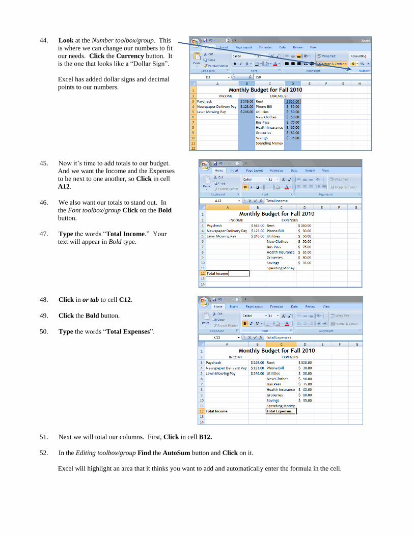
24. Using your arrow keys, move into cell A2 and Type ―This is cell A2‖. Move into cell B2 and
Type ―This is cell B2”, move into cell C2 and Type ―This is cell C2‖.
25. Select all of the text and change the font to Times New Roman 14 pt. Note: to use these tools
you must be on the Home tab of the Ribbon in the Font toolbox.
Click and Drag
26. Bold the text. This tool is also found in the Font toolbox.
27. Click on the corner button to select the entire worksheet.
28. Double-click between the column labels to resize all the columns at the same time.
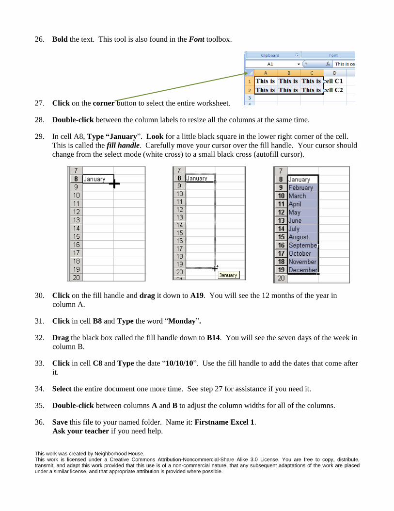
29. In cell A8, Type “January‖. Look for a little black square in the lower right corner of the cell.
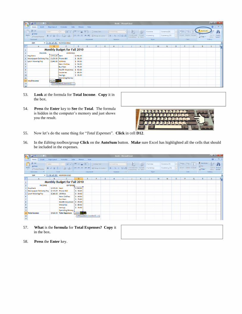
This is called the fill handle. Carefully move your cursor over the fill handle. Your cursor should
change from the select mode (white cross) to a small black cross (autofill cursor).
30. Click on the fill handle and drag it down to A19. You will see the 12 months of the year in
column A.
31. Click in cell B8 and Type the word ―Monday‖.
32. Drag the black box called the fill handle down to B14. You will see the seven days of the week in
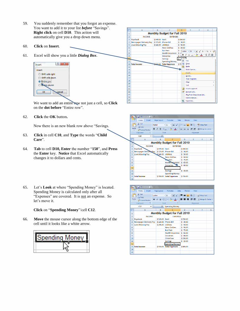
column B.
33. Click in cell C8 and Type the date ―10/10/10‖. Use the fill handle to add the dates that come after
it.
34. Select the entire document one more time. See step 27 for assistance if you need it.
35. Double-click between columns A and B to adjust the column widths for all of the columns.
36. Save this file to your named folder. Name it: Firstname Excel 1.
Ask your teacher if you need help.
This work was created by Neighborhood House. This work is licensed under a Creative Commons Attribution-Noncommercial-Share Alike 3.0 License. You are free to copy, distribute, transmit, and adapt this work provided that this use is of a non-commercial nature, that any subsequent adaptations of the work are placed under a similar license, and that appropriate attribution is provided where possible.
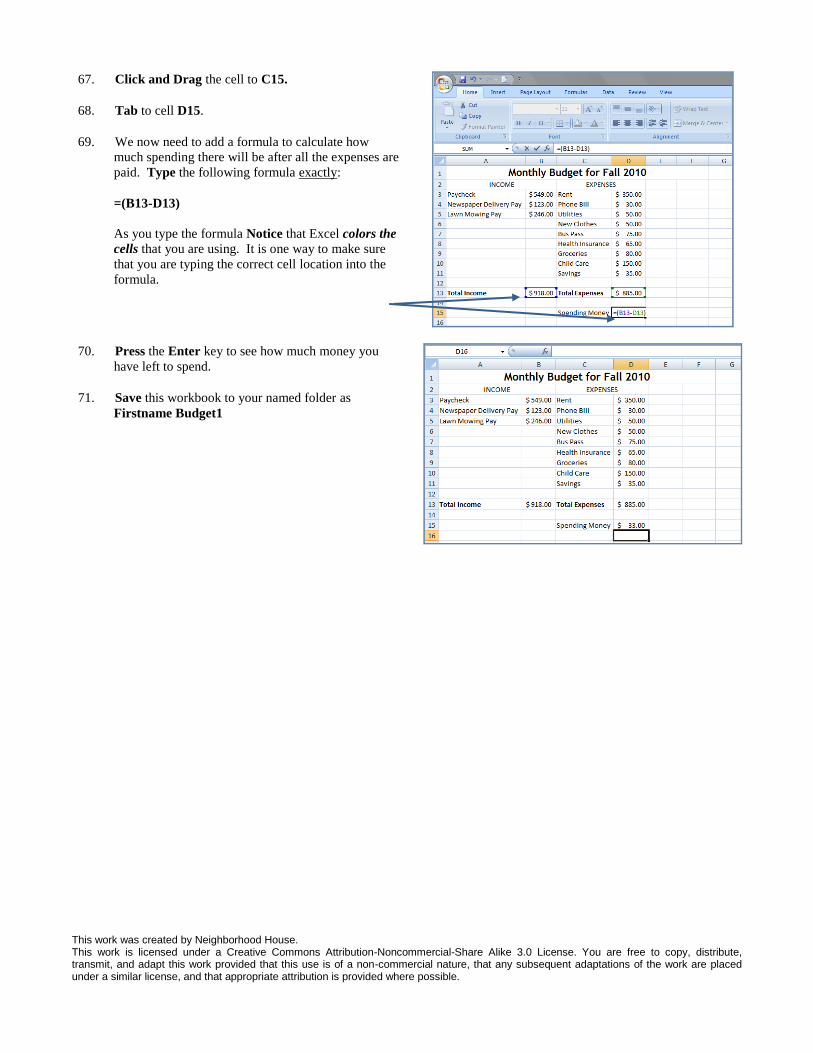
Microsoft Excel: Exercise 2
Making Lists
In this exercise:
Moving from one cell to another
Entering information in cells
Removing a hyperlink
Center and merge
Sort ascending
Deleting a row or column
1. Open a new Excel workbook by doing one of the following:
a. Click the Start button, Click on All Programs, Microsoft Office, Microsoft Excel
b. Click the Start button, if Microsoft Excel is in the first list, click on it.
c. Click the Microsoft Excel Shortcut on the Desktop.
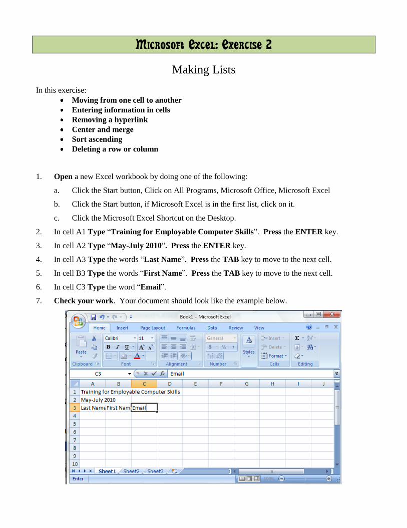
2. In cell A1 Type ―Training for Employable Computer Skills‖. Press the ENTER key.
3. In cell A2 Type ―May-July 2010‖. Press the ENTER key.
4. In cell A3 Type the words ―Last Name‖. Press the TAB key to move to the next cell.
5. In cell B3 Type the words ―First Name‖. Press the TAB key to move to the next cell.
6. In cell C3 Type the word ―Email‖.
7. Check your work. Your document should look like the example below.
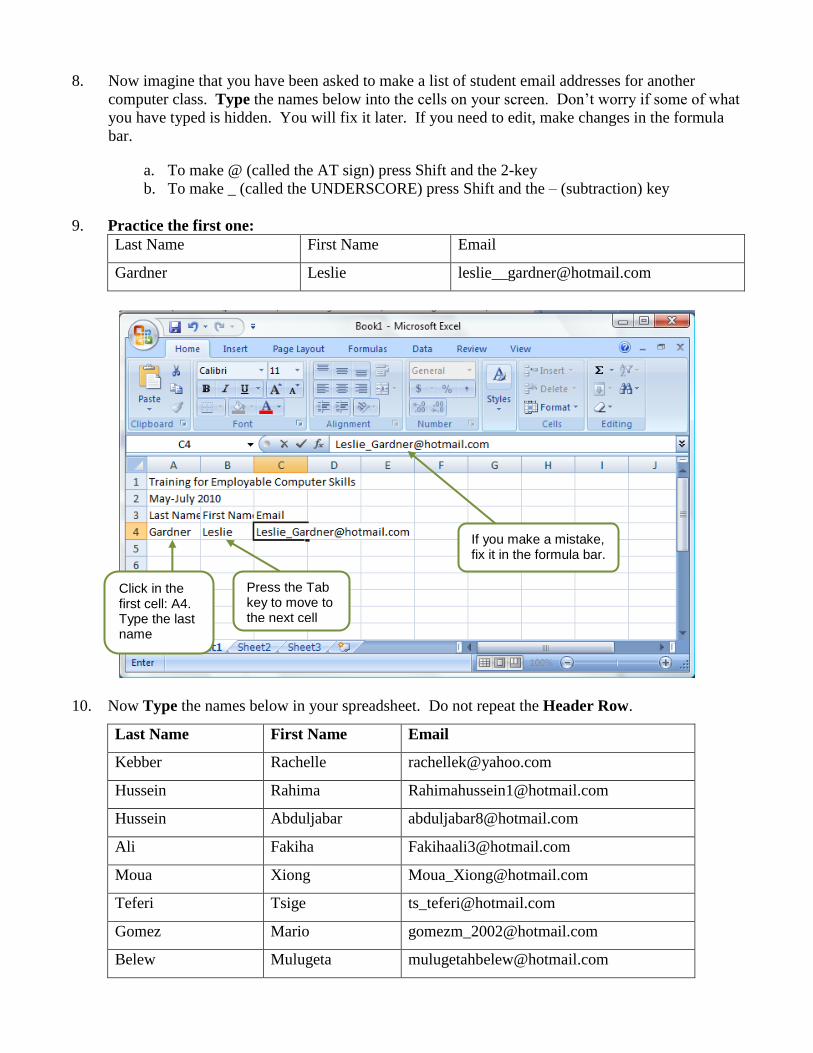
8. Now imagine that you have been asked to make a list of student email addresses for another
computer class. Type the names below into the cells on your screen. Don’t worry if some of what
you have typed is hidden. You will fix it later. If you need to edit, make changes in the formula
bar.
a. To make @ (called the AT sign) press Shift and the 2-key
b. To make _ (called the UNDERSCORE) press Shift and the – (subtraction) key
9. Practice the first one:
Last Name First Name Email
Gardner Leslie [email protected]
10. Now Type the names below in your spreadsheet. Do not repeat the Header Row.
Last Name First Name Email
Kebber Rachelle [email protected]
Hussein Rahima [email protected]
Hussein Abduljabar [email protected]
Ali Fakiha [email protected]
Moua Xiong [email protected]
Teferi Tsige [email protected]
Gomez Mario [email protected]
Belew Mulugeta [email protected]
Click in the first cell: A4. Type the last name
Press the Tab key to move to the next cell
If you make a mistake, fix it in the formula bar.
Last Name First Name Email
Brown John [email protected]
Mohamed Abdullahi [email protected]
Kifleyesus Selamawit [email protected]
Asfaw Tsehay [email protected]
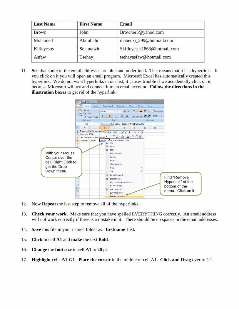
11. See that some of the email addresses are blue and underlined. That means that it is a hyperlink. If
you click on it you will open an email program. Microsoft Excel has automatically created this
hyperlink. We do not want hyperlinks in our list; it causes trouble if we accidentally click on it,
because Microsoft will try and connect it to an email account. Follow the directions in the
illustration boxes to get rid of the hyperlink.
12. Now Repeat the last step to remove all of the hyperlinks.
13. Check your work. Make sure that you have spelled EVERYTHING correctly. An email address
will not work correctly if there is a mistake in it. There should be no spaces in the email addresses.
14. Save this file in your named folder as: firstname List.
15. Click in cell A1 and make the text Bold.
16. Change the font size in cell A1 to 20 pt.
17. Highlight cells A1-G1. Place the cursor in the middle of cell A1. Click and Drag over to G1.
With your Mouse Cursor over the cell, Right Click to get the Drop Down menu.
Find “Remove Hyperlink” at the bottom of the menu. Click on it.
18. Click on the center and merge button located in your toolbar.
Merge and Center changes many cells into one cell.
Excel will also center the text in the middle of this merged cell.
19. Change the font size in cell A2 to 14 pt and Make it Bold.
20. Highlight cells A2 to G2 and Click on the center and merge button.
21. Double click on the line between the labels for Column A and B. Excel will automatically re-size
the column to fit the text.
22. Repeat the same thing between column B and C, and C and D
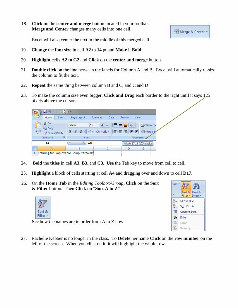
23. To make the column size even bigger, Click and Drag each border to the right until it says 125
pixels above the cursor.
24. Bold the titles in cell A3, B3, and C3. Use the Tab key to move from cell to cell.
25. Highlight a block of cells starting at cell A4 and dragging over and down to cell D17.
26. On the Home Tab in the Editing Toolbox/Group, Click on the Sort
& Filter button. Then Click on ―Sort A to Z‖
See how the names are in order from A to Z now.
27. Rachelle Kebber is no longer in the class. To Delete her name Click on the row number on the
left of the screen. When you click on it, it will highlight the whole row.
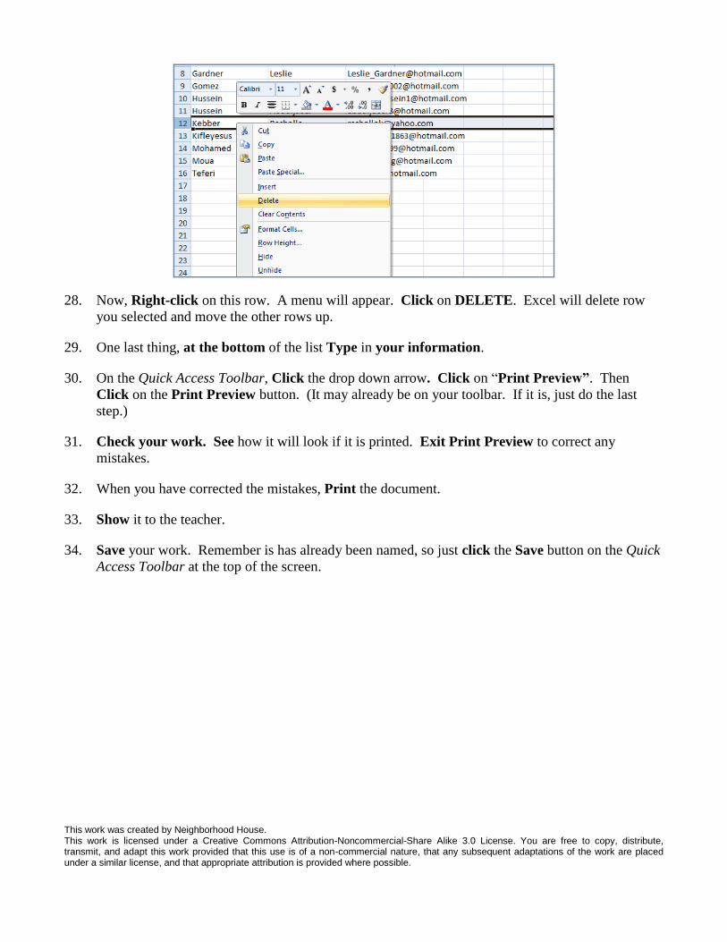
28. Now, Right-click on this row. A menu will appear. Click on DELETE. Excel will delete row
you selected and move the other rows up.
29. One last thing, at the bottom of the list Type in your information.
30. On the Quick Access Toolbar, Click the drop down arrow. Click on ―Print Preview”. Then
Click on the Print Preview button. (It may already be on your toolbar. If it is, just do the last
step.)
31. Check your work. See how it will look if it is printed. Exit Print Preview to correct any
mistakes.
32. When you have corrected the mistakes, Print the document.
33. Show it to the teacher.
34. Save your work. Remember is has already been named, so just click the Save button on the Quick
Access Toolbar at the top of the screen.
This work was created by Neighborhood House. This work is licensed under a Creative Commons Attribution-Noncommercial-Share Alike 3.0 License. You are free to copy, distribute, transmit, and adapt this work provided that this use is of a non-commercial nature, that any subsequent adaptations of the work are placed under a similar license, and that appropriate attribution is provided where possible.

Microsoft Excel: Exercise 3
Budgets 1
1. Open Microsoft Excel. The ―Box‖ cursor
should already be in cell A1. If not, Click
in cell A1.
2. Type the words ―Monthly Budget for
Fall 2010‖.
3. Press the down arrow key.
4. Type the word ―INCOME‖. Use all
capital/uppercase letters. You can either
Hold down the Shift key as you type, or
Use the Caps Lock key.
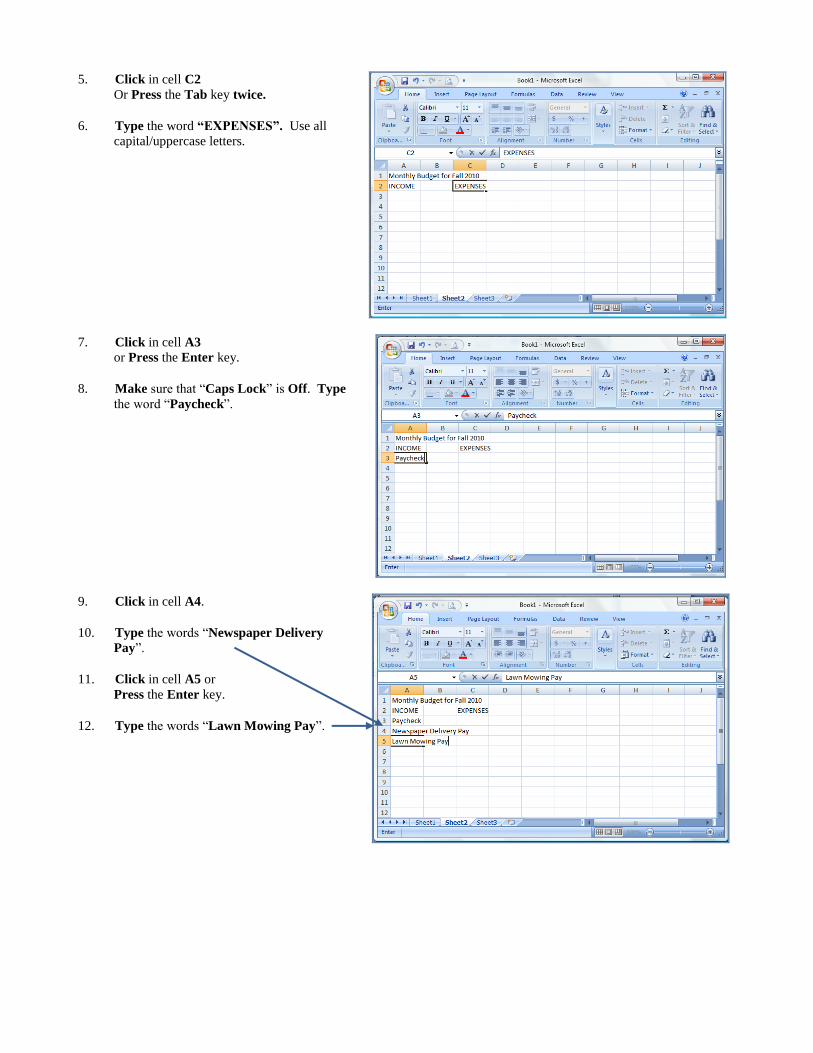
5. Click in cell C2
Or Press the Tab key twice.
6. Type the word “EXPENSES”. Use all
capital/uppercase letters.
7. Click in cell A3
or Press the Enter key.
8. Make sure that ―Caps Lock‖ is Off. Type
the word ―Paycheck‖.
9. Click in cell A4.
10. Type the words ―Newspaper Delivery
Pay‖.
11. Click in cell A5 or
Press the Enter key.
12. Type the words ―Lawn Mowing Pay‖.
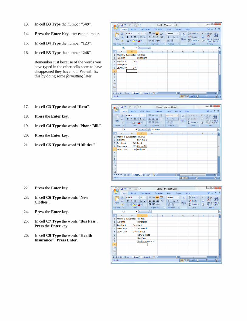
13. In cell B3 Type the number ―549‖.
14. Press the Enter Key after each number.
15. In cell B4 Type the number ―123‖.
16. In cell B5 Type the number ―246‖.
Remember just because of the words you
have typed in the other cells seem to have
disappeared they have not. We will fix
this by doing some formatting later.
17. In cell C3 Type the word ―Rent‖.
18. Press the Enter key.
19. In cell C4 Type the words ―Phone Bill.‖
20. Press the Enter key.
21. In cell C5 Type the word ―Utilities.‖
22. Press the Enter key.
23. In cell C6 Type the words ―New
Clothes‖.
24. Press the Enter key.
25. In cell C7 Type the words ―Bus Pass‖.
Press the Enter key.
26. In cell C8 Type the words ―Health
Insurance‖. Press Enter.
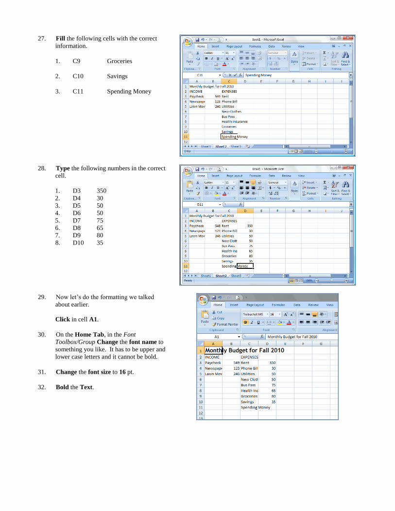
27. Fill the following cells with the correct
information.
1. C9 Groceries
2. C10 Savings
3. C11 Spending Money
28. Type the following numbers in the correct
cell.
1. D3 350
2. D4 30
3. D5 50
4. D6 50
5. D7 75
6. D8 65
7. D9 80
8. D10 35
29. Now let’s do the formatting we talked
about earlier.
Click in cell A1.
30. On the Home Tab, in the Font
Toolbox/Group Change the font name to
something you like. It has to be upper and
lower case letters and it cannot be bold.
31. Change the font size to 16 pt.
32. Bold the Text.
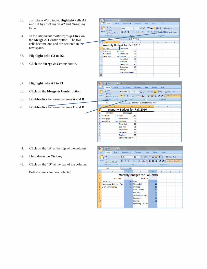
33. Just like a Word table, Highlight cells A2
and B2 by Clicking on A2 and Dragging
to B2.
34. In the Alignment toolbox/group Click on
the Merge & Center button. The two
cells become one and are centered in the
new space.
35. Highlight cells C2 to D2.
36. Click the Merge & Center button.
37. Highlight cells A1 to F1.
38. Click on the Merge & Center button.
39. Double-click between columns A and B.
40. Double-click between columns C and D.
41. Click on the ―B‖ at the top of the column.
42. Hold down the Ctrl key.
43. Click on the ―D‖ at the top of the column.
Both columns are now selected.
44. Look at the Number toolbox/group. This
is where we can change our numbers to fit
our needs. Click the Currency button. It
is the one that looks like a ―Dollar Sign‖.
Excel has added dollar signs and decimal
points to our numbers.
45. Now it’s time to add totals to our budget.
And we want the Income and the Expenses
to be next to one another, so Click in cell
A12.
46. We also want our totals to stand out. In
the Font toolbox/group Click on the Bold
button.
47. Type the words ―Total Income.‖ Your
text will appear in Bold type.
48. Click in or tab to cell C12.
49. Click the Bold button.
50. Type the words ―Total Expenses‖.
51. Next we will total our columns. First, Click in cell B12.
52. In the Editing toolbox/group Find the AutoSum button and Click on it.
Excel will highlight an area that it thinks you want to add and automatically enter the formula in the cell.
53. Look at the formula for Total Income. Copy it in
the box.
54. Press the Enter key to See the Total. The formula
is hidden in the computer’s memory and just shows
you the result.
55. Now let’s do the same thing for ―Total Expenses‖. Click in cell D12.
56. In the Editing toolbox/group Click on the AutoSum button. Make sure Excel has highlighted all the cells that should
be included in the expenses.
57. What is the formula for Total Expenses? Copy it
in the box.
58. Press the Enter key.
59. You suddenly remember that you forgot an expense.
You want to add it to your list before ―Savings‖.
Right click on cell D10. This action will
automatically give you a drop down menu.
60. Click on Insert.
61. Excel will show you a little Dialog Box.
We want to add an entire row not just a cell, so Click
on the dot before ―Entire row‖.
62. Click the OK button.
Now there is an new blank row above ―Savings.
63. Click in cell C10, and Type the words ―Child
Care‖.
64. Tab to cell D10, Enter the number ―150‖, and Press
the Enter key. Notice that Excel automatically
changes it to dollars and cents.
65. Let’s Look at where ―Spending Money‖ is located.
Spending Money is calculated only after all
―Expenses‖ are covered. It is not an expense. So
let’s move it.
Click on ―Spending Money‖/cell C12.
66. Move the mouse cursor along the bottom edge of the
cell until it looks like a white arrow.
67. Click and Drag the cell to C15.
68. Tab to cell D15.
69. We now need to add a formula to calculate how
much spending there will be after all the expenses are
paid. Type the following formula exactly:
=(B13-D13)
As you type the formula Notice that Excel colors the
cells that you are using. It is one way to make sure
that you are typing the correct cell location into the
formula.
70. Press the Enter key to see how much money you
have left to spend.
71. Save this workbook to your named folder as
Firstname Budget1
This work was created by Neighborhood House. This work is licensed under a Creative Commons Attribution-Noncommercial-Share Alike 3.0 License. You are free to copy, distribute, transmit, and adapt this work provided that this use is of a non-commercial nature, that any subsequent adaptations of the work are placed under a similar license, and that appropriate attribution is provided where possible.
Microsoft Excel: Exercise 5
Making Charts 1
In this exercise:
Using AutoSum
Using the fill handle to copy formulas
Using AutoFormat
Using the Chart Wizard to create a pie and bar graph
Building a Spreadsheet.
This is a case study exercise. In a case study you imagine that you are doing work for an actual job.
Read the information in the box below.
Case Study
While traveling in Mexico, Sarah Voyage and three of her friends came up with the idea of starting a
worldwide travel agency for college students. After graduation, they invested $3,000 each and started
their dream company, Spring Break Travels, Inc. Thanks to their good business skills and the popularity
of personal computers and the World Wide Web, the company has become the number one for college
Spring Break trips.
As sales continue to grow, the management at Spring Break Travels, Inc. has realized they need a better
tracking system for first quarter sales. As a result, they have asked you to prepare a first quarter sales
worksheet that shows the sales for the first quarter.
In addition, Sarah has asked you to create 2 graphs showing the first quarter sales (a pie graph showing
the most effective sales method and a bar graph showing the most popular vacation packages) since she
does not like only lists of numbers.
1. Click on cell A1
2. Type Spring Break Travels 1st Qtr Sales in cell A1. This is the title of your spreadsheet.
3. Click on cell B2
4. Type Mail
5. Press the right arrow key to move to cell C2
6. Type Campus in C2, Telephone in D2, Web in E2, and Total in F2. These are all the ways that the
company advertises.
7. Click on cell A3 and Type Bahamas Beach Party. Press the key.
8. Type Florida Vacation in cell A4, St. Thomas Escape in cell A5, South Padre Paradise in cell A6
and Total in cell A7.
9. Type these numbers in the correct cells:
Mail Campus Telephone Web
Bahamas Beach 52978.23 38781.35 37213.45 29998.65
Florida Vacation 28234.5 48401.53 27034.56 42911.16
St. Thomas Escape 62567.25 72516.12 24354.86 77019.32
South Padre Paradise 28567.15 69777.64 49976.6 32019.45
10. Click on cell B7, and then Click on the AutoSum button on the Home Tab in the Editing group.
It looks like this:
Column B will be surrounded by a moving border called a marquee. The formula =SUM(B3:B6)
will appear in cell B7.
11. Click the AutoSum button again. A total will appear. The computer has added together all the
numbers in cells B3, B4, B5, B6.
12. Click in cell B7, Place the cursor over the fill handle (the tiny black square at the bottom right of
the selected cell) and drag the cursor to cell E7.
13. Take your finger off the mouse button. Excel has automatically added together each one of the
columns. You can see how much money was made through each type of advertising (mail,
campus, web etc.)
14. Click on cell F3. Highlight the column down to F7 (do not use the fill handle).
15. Click on the AutoSum button. Now you have added up the total amount of money made at each
vacation place.
16. Click in B5. Type the number 12.
17. Press the ENTER key. See that Excel automatically changes the total to the format we selected.
18. Highlight B3 to F7. In the Number toolbox, Click on the down arrow next to the word ―General‖.
19. On the drop down menu, Click on Accounting. See how Excel automatically formats your spreadsheet.
20. Click in cell A1 and Highlight until F1. Press the center and merge button. Bold the title and Change the font size
to 16pt.
21. Bold the words Mail, Campus, Telephone, Web and also the names for the tours.
22. Double-click between the A and B at the top of the column.
23. Highlight the columns labeled ―B‖ to ―F‖. While it is highlight, double-click between any of the
highlighted columns. This will change the width of each column.
24. Save this workbook in your named folder as Firstname Charts1. Do not close.
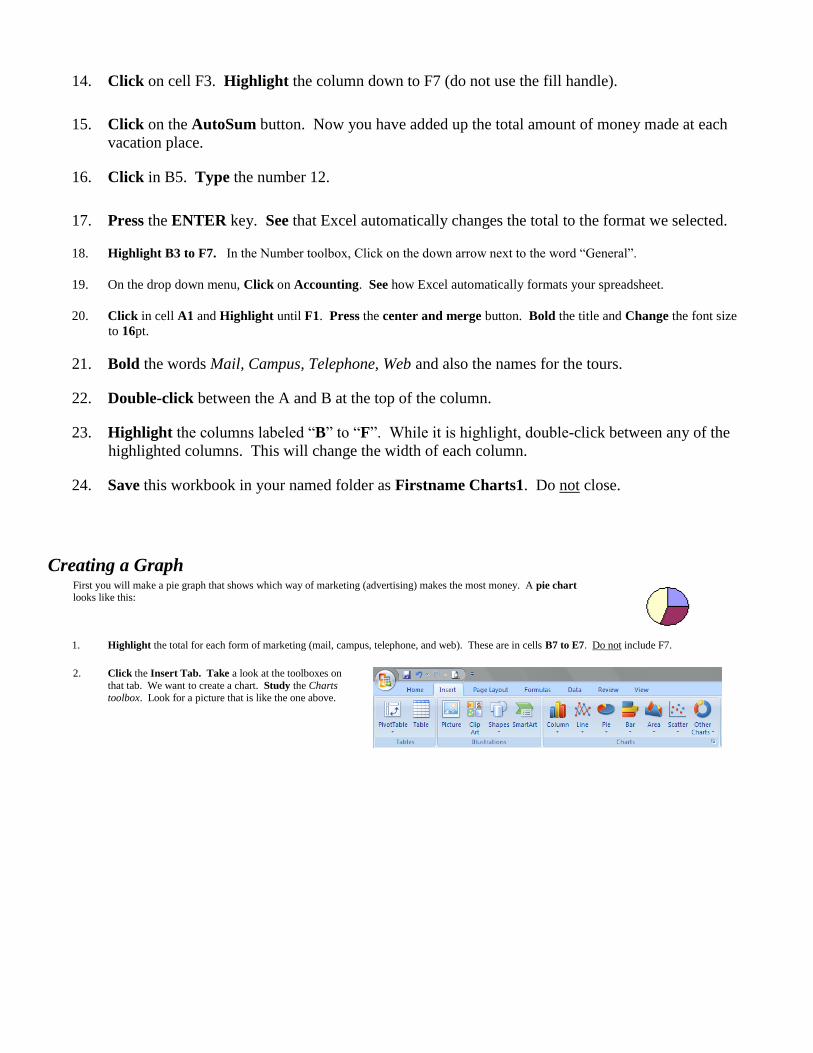
Creating a Graph First you will make a pie graph that shows which way of marketing (advertising) makes the most money. A pie chart looks like this:
1. Highlight the total for each form of marketing (mail, campus, telephone, and web). These are in cells B7 to E7. Do not include F7.
2. Click the Insert Tab. Take a look at the toolboxes on
that tab. We want to create a chart. Study the Charts
toolbox. Look for a picture that is like the one above.
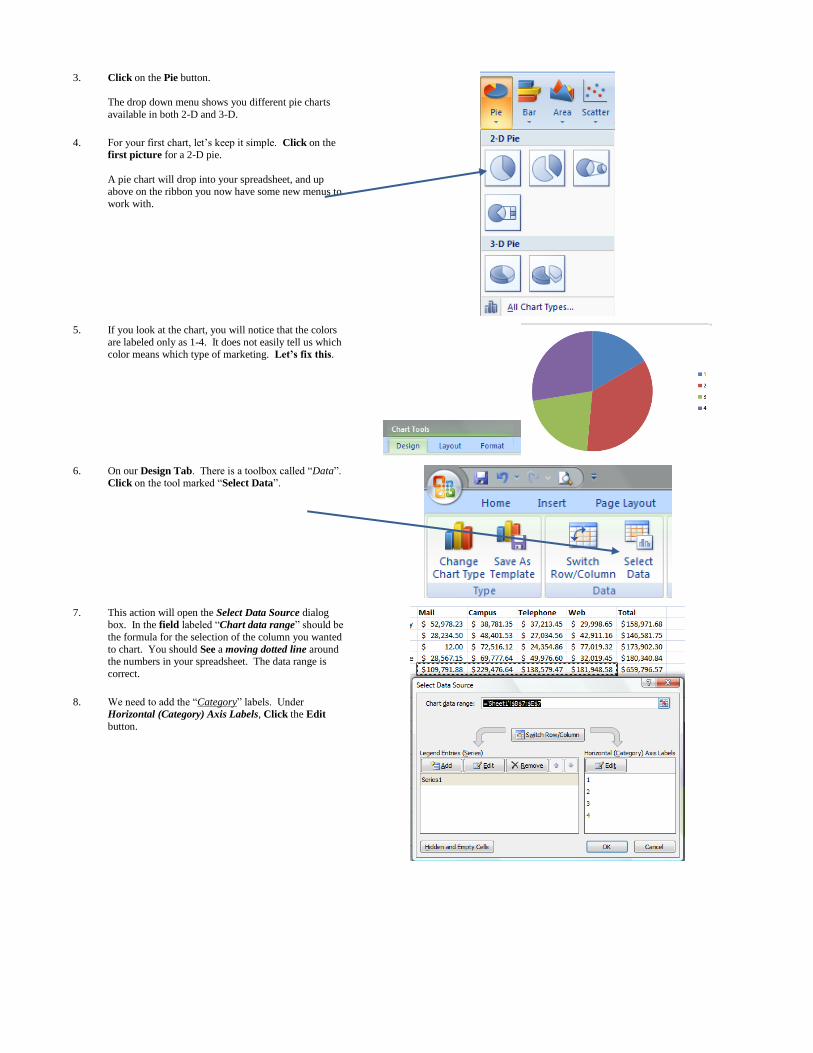
3. Click on the Pie button.
The drop down menu shows you different pie charts
available in both 2-D and 3-D.
4. For your first chart, let’s keep it simple. Click on the first picture for a 2-D pie.
A pie chart will drop into your spreadsheet, and up above on the ribbon you now have some new menus to
work with.
5. If you look at the chart, you will notice that the colors
are labeled only as 1-4. It does not easily tell us which color means which type of marketing. Let’s fix this.
6. On our Design Tab. There is a toolbox called ―Data‖. Click on the tool marked ―Select Data‖.
7. This action will open the Select Data Source dialog box. In the field labeled ―Chart data range‖ should be
the formula for the selection of the column you wanted
to chart. You should See a moving dotted line around the numbers in your spreadsheet. The data range is
correct.
8. We need to add the ―Category‖ labels. Under
Horizontal (Category) Axis Labels, Click the Edit
button.
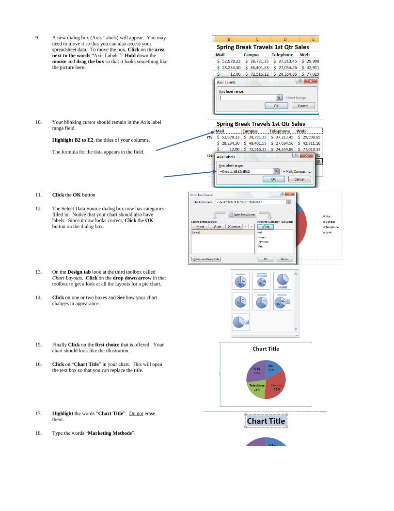
9. A new dialog box (Axis Labels) will appear. You may
need to move it so that you can also access your
spreadsheet data. To move the box, Click on the area
next to the words ―Axis Labels‖. Hold down the
mouse and drag the box so that it looks something like the picture here:
10. Your blinking cursor should remain in the Axis label range field.
Highlight B2 to E2, the titles of your columns.
The formula for the data appears in the field.
11. Click the OK button
12. The Select Data Source dialog box now has categories
filled in. Notice that your chart should also have labels. Since it now looks correct, Click the OK
button on the dialog box.
13. On the Design tab look at the third toolbox called
Chart Layouts. Click on the drop down arrow in that
toolbox to get a look at all the layouts for a pie chart.
14. Click on one or two boxes and See how your chart
changes in appearance.
15. Finally Click on the first choice that is offered. Your
chart should look like the illustration.
16. Click on ―Chart Title‖ in your chart. This will open
the text box so that you can replace the title.
17. Highlight the words ―Chart Title‖. Do not erase
them.
18. Type the words ―Marketing Methods‖.
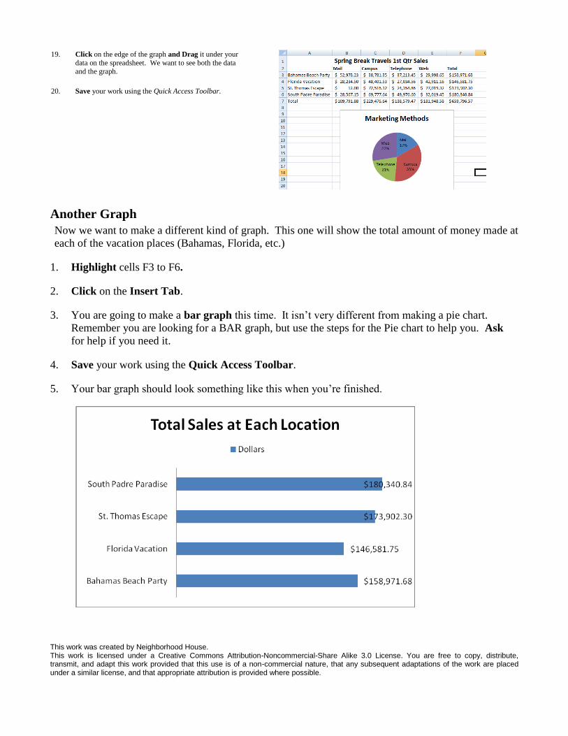
19. Click on the edge of the graph and Drag it under your
data on the spreadsheet. We want to see both the data
and the graph.
20. Save your work using the Quick Access Toolbar.
Another Graph
Now we want to make a different kind of graph. This one will show the total amount of money made at
each of the vacation places (Bahamas, Florida, etc.)
1. Highlight cells F3 to F6.
2. Click on the Insert Tab.
3. You are going to make a bar graph this time. It isn’t very different from making a pie chart.
Remember you are looking for a BAR graph, but use the steps for the Pie chart to help you. Ask
for help if you need it.
4. Save your work using the Quick Access Toolbar.
5. Your bar graph should look something like this when you’re finished.
This work was created by Neighborhood House. This work is licensed under a Creative Commons Attribution-Noncommercial-Share Alike 3.0 License. You are free to copy, distribute, transmit, and adapt this work provided that this use is of a non-commercial nature, that any subsequent adaptations of the work are placed under a similar license, and that appropriate attribution is provided where possible.

Microsoft Excel: Exercise 6
Using Excel on Your Own
Budget 2
This activity is a test to see how well you understand Microsoft Excel and the spreadsheet format.
I would like you to create a monthly budget for an imaginary person named Fred.
This budget will need separate columns for expenses and income.
You should show totals for the expenses and income.
Also show what Fred will have left over by subtracting his total expenses from the total income.
This is Fred’s spending money.
Finally make a bar graph that compares Fred’s monthly expenses with his monthly income.
Good Luck!
Below is the information about how much money Fred earns each month and how much he spends.
Fred earns $123.00 a month delivering newspapers. He earns $246.00 a month mowing lawns. He
earns $549.00 per month stocking shelves at a grocery store.
Fred spends $350.00 a month on rent. He spends about $30.00 a month on phone bills. He spends
$50.00 a month on utilities like heat and electricity. He needs to buy new shoes this month so that will
cost an extra $50.00. He spends about $80.00 a month on groceries. And he tries to save at least $35.00
a month in his savings account. He does not have to pay for gas or car repairs but he does spend about
$75.00 a month on the bus. He also pays for health insurance, which costs $65.00 per month. Decide
what a reasonable amount for Fred to spend on fun things like eating out, movies, and buying new stuff.
You can make this one category in his budget.
Save this document in your named folder as Firstname Budget2
HINT: When it comes to creating the graph/chart for Fred’s Budget, you will need to do the following
steps:
1. Select the Total amount of Fred’s Income—the dollar amount only.
2. Hold down the Ctrl (Control) key.
3. Select the Total amount of Fred’s Expenses—the dollar amount only.
4. Then Click the Insert Tab and choose a simple bar graph/chart.
Use your previous exercises to help you complete the graph. This work was created by Neighborhood House. This work is licensed under a Creative Commons Attribution-Noncommercial-Share Alike 3.0 License. You are free to copy, distribute, transmit, and adapt this work provided that this use is of a non-commercial nature, that any subsequent adaptations of the work are placed under a similar license, and that appropriate attribution is provided where possible.
Microsoft Excel: Exercise 7
Making Charts 2
In this exercise you will collect some information from other people in the class. You will use the information to make a
table and graphs in Microsoft Excel.
1. Ask every person in the classroom (including teachers):
a. What country were you born in?
b. What languages do you speak? (Some people may speak more
than one language. Klingon does count as a language.)
2. Write down the answers on a piece of paper.
3. Open Microsoft Excel.
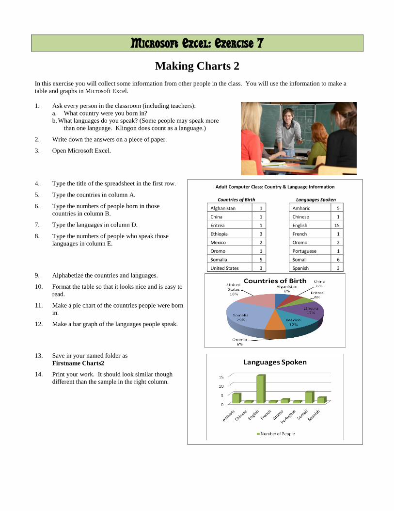
4. Type the title of the spreadsheet in the first row.
5. Type the countries in column A.
6. Type the numbers of people born in those
countries in column B.
7. Type the languages in column D.
8. Type the numbers of people who speak those
languages in column E.
Adult Computer Class: Country & Language Information
Countries of Birth
Languages Spoken
Afghanistan 1
Amharic 5
China 1
Chinese 1
Eritrea 1
English 15
Ethiopia 3
French 1
Mexico 2
Oromo 2
Oromo 1
Portuguese 1
Somalia 5
Somali 6
United States 3
Spanish 3
9. Alphabetize the countries and languages.
10. Format the table so that it looks nice and is easy to
read.
11. Make a pie chart of the countries people were born
in.
12. Make a bar graph of the languages people speak.
13. Save in your named folder as
Firstname Charts2
14. Print your work. It should look similar though
different than the sample in the right column.

This work was created by Neighborhood House. This work is licensed under a Creative Commons Attribution-Noncommercial-Share Alike 3.0 License. You are free to copy, distribute, transmit, and adapt this work provided that this use is of a non-commercial nature, that any subsequent adaptations of the work are placed under a similar license, and that appropriate attribution is provided where possible.