Microsoft Excel 2003 - Department of Psychology ... · Microsoft Excel 2003 Data Analysis ... Using Excel’s Data Analysis Tools Excel includes a number of add-in tools to assist

Microsoft Excel 2003

Data Analysis

Larry F. Vint, Ph.D [email protected] 815-753-8053

Technical Advisory Group

Customer Support Services Northern Illinois University

120 Swen Parson Hall DeKalb, IL 60115

© Copyright 2004 Northern Illinois University Information Technology Services

© Copyright 2004 Northern Illinois University Information Technology Services 1

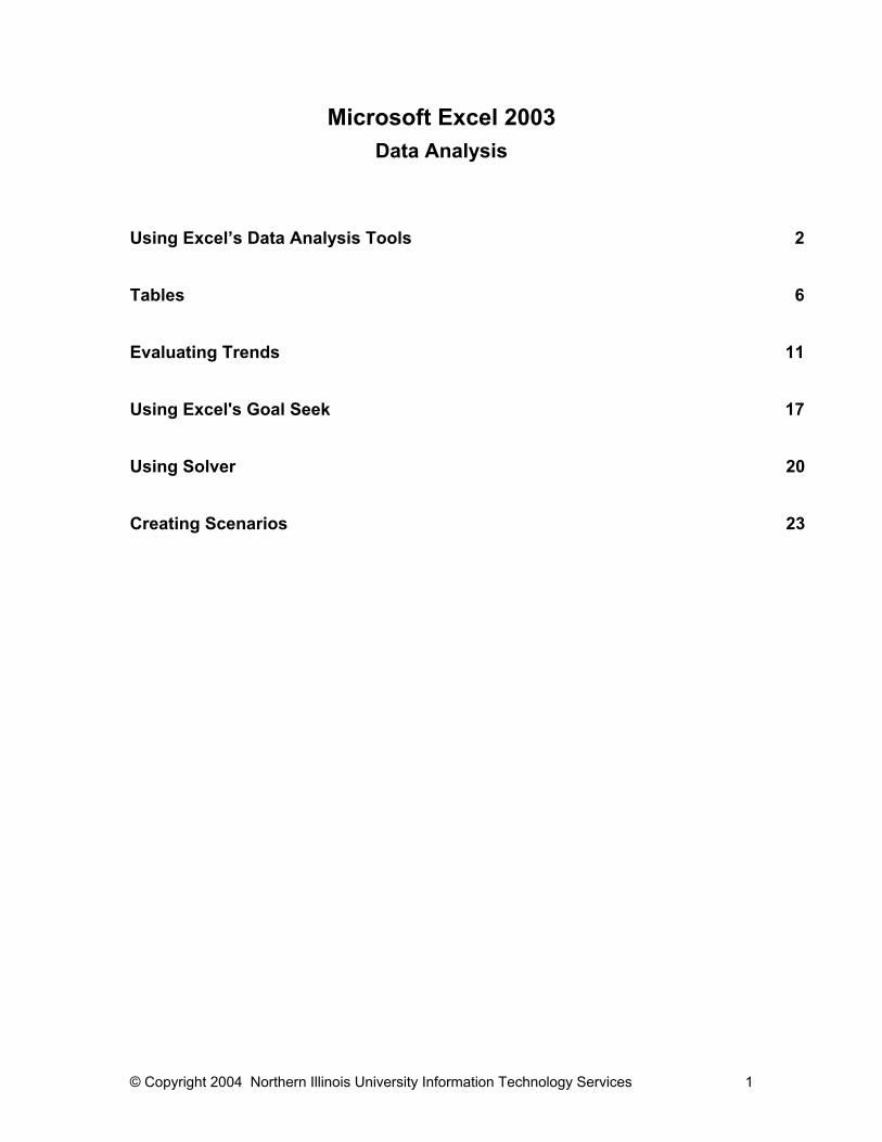
Microsoft Excel 2003 Data Analysis

Using Excel’s Data Analysis Tools 2 Tables 6 Evaluating Trends 11 Using Excel's Goal Seek 17 Using Solver 20 Creating Scenarios 23


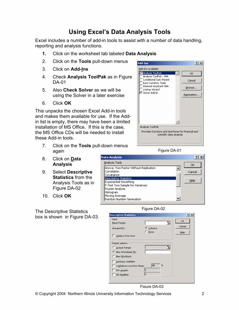
Using Excel’s Data Analysis Tools Excel includes a number of add-in tools to assist with a number of data handling, reporting and analysis functions.

1. Click on the worksheet tab labeled Data Analysis 2. Click on the Tools pull-down menus 3. Click on Add-Ins 4. Check Analysis ToolPak as in Figure

DA-01 5. Also Check Solver as we will be

using the Solver in a later exercise 6. Click OK

This unpacks the chosen Excel Add-in tools and makes them available for use. If the Add-in list is empty, there may have been a limited installation of MS Office. If this is the case, the MS Office CDs will be needed to install these Add-in tools.

7. Click on the Tools pull-down menus again

8. Click on Data Analysis

9. Select Descriptive Statistics from the Analysis Tools as in Figure DA-02

10. Click OK The Descriptive Statistics box is shown in Figure DA-03.

Figure DA-01

Figure DA-02

Figure DA-03


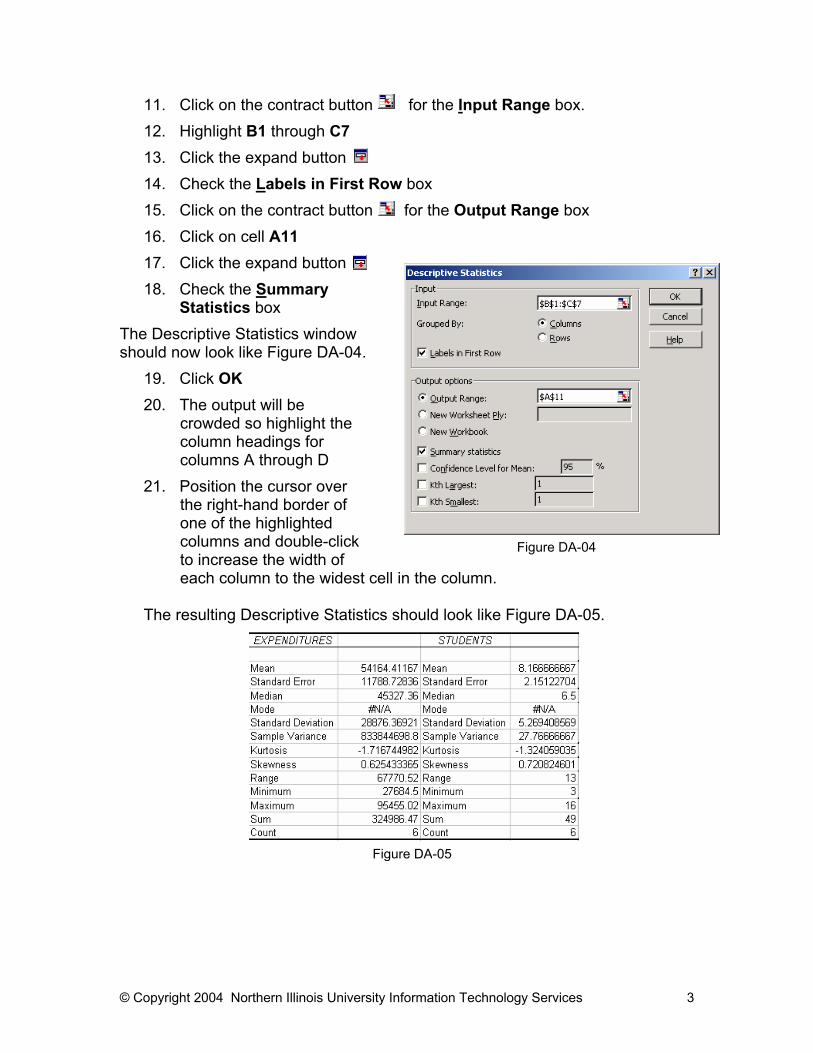
11. Click on the contract button for the Input Range box. 12. Highlight B1 through C7 13. Click the expand button 14. Check the Labels in First Row box 15. Click on the contract button for the Output Range box 16. Click on cell A11 17. Click the expand button 18. Check the Summary

Statistics box The Descriptive Statistics window should now look like Figure DA-04.

19. Click OK 20. The output will be

crowded so highlight the column headings for columns A through D

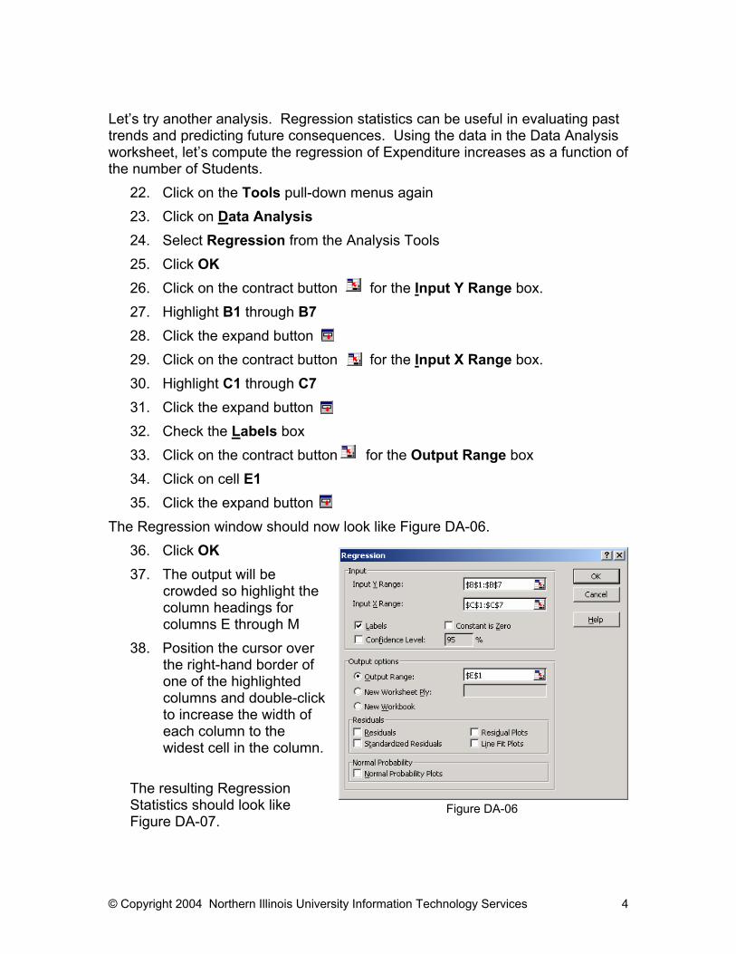
21. Position the cursor over the right-hand border of one of the highlighted columns and double-click to increase the width of each column to the widest cell in the column.

The resulting Descriptive Statistics should look like Figure DA-05.

Figure DA-05

Figure DA-04


Let’s try another analysis. Regression statistics can be useful in evaluating past trends and predicting future consequences. Using the data in the Data Analysis worksheet, let’s compute the regression of Expenditure increases as a function of the number of Students.

22. Click on the Tools pull-down menus again 23. Click on Data Analysis 24. Select Regression from the Analysis Tools 25. Click OK 26. Click on the contract button for the Input Y Range box. 27. Highlight B1 through B7 28. Click the expand button 29. Click on the contract button for the Input X Range box. 30. Highlight C1 through C7 31. Click the expand button 32. Check the Labels box 33. Click on the contract button for the Output Range box 34. Click on cell E1 35. Click the expand button

The Regression window should now look like Figure DA-06. 36. Click OK 37. The output will be

crowded so highlight the column headings for columns E through M

38. Position the cursor over the right-hand border of one of the highlighted columns and double-click to increase the width of each column to the widest cell in the column.

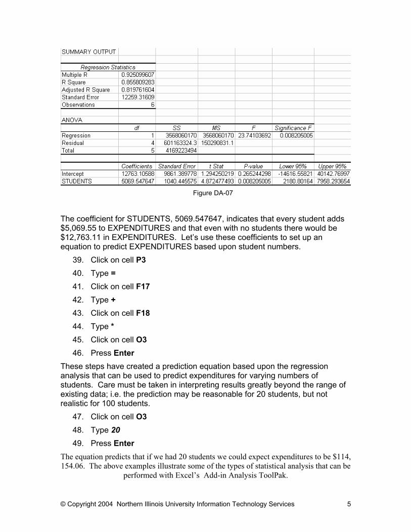
The resulting Regression Statistics should look like Figure DA-07.

Figure DA-06


The coefficient for STUDENTS, 5069.547647, indicates that every student adds $5,069.55 to EXPENDITURES and that even with no students there would be $12,763.11 in EXPENDITURES. Let’s use these coefficients to set up an equation to predict EXPENDITURES based upon student numbers.

39. Click on cell P3 40. Type = 41. Click on cell F17 42. Type + 43. Click on cell F18 44. Type * 45. Click on cell O3 46. Press Enter

These steps have created a prediction equation based upon the regression analysis that can be used to predict expenditures for varying numbers of students. Care must be taken in interpreting results greatly beyond the range of existing data; i.e. the prediction may be reasonable for 20 students, but not realistic for 100 students.

47. Click on cell O3 48. Type 20 49. Press Enter

The equation predicts that if we had 20 students we could expect expenditures to be $114, 154.06. The above examples illustrate some of the types of statistical analysis that can be

performed with Excel’s Add-in Analysis ToolPak.

Figure DA-07


Tables Most people familiar with databases will mistakenly assume the Tables feature in Excel is used similarly but they are mistaken. The Tables feature in Excel is another What-If analysis tool that displays the result of a formula with different sets of input values. For this example we will create a formula that determines the monthly payments for the principal of an investment given a fixed interest rate. We will use the PPMT function that is one of the financial functions provided by Excel to calculate the monthly payments to be made on an investment over a specified period of time. We will enter the interest rate, Let’s first go to the Payment Table worksheet for the function and ensuing table.

1. Click on the Payment Table worksheet tab Let’s enter the input values for the function first and then create the function.

2. Click on cell B1 3. Type 7.5 4. Click on cell B2 5. Type 5 6. Click on cell B3 7. Type 18000

These three values will be used by the PMT function to calculate the monthly payments. Let’s enter the formula.

8. Click on cell B6 9. Click on the Paste Function toolbar button 10. From popup Insert Function window click on the Financial category

from the select a category pick list

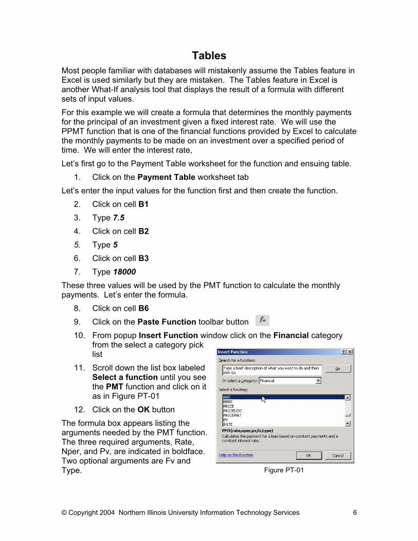
11. Scroll down the list box labeled Select a function until you see the PMT function and click on it as in Figure PT-01

12. Click on the OK button The formula box appears listing the arguments needed by the PMT function. The three required arguments, Rate, Nper, and Pv, are indicated in boldface. Two optional arguments are Fv and Type. Figure PT-01


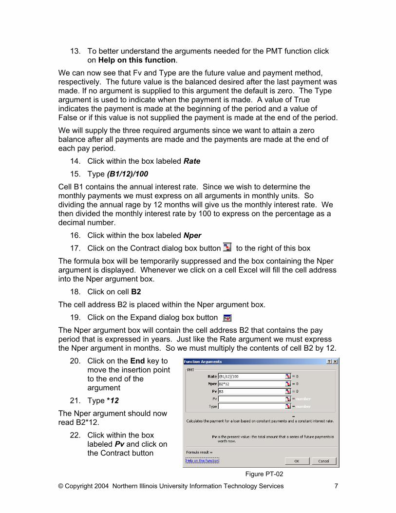
13. To better understand the arguments needed for the PMT function click on Help on this function.

We can now see that Fv and Type are the future value and payment method, respectively. The future value is the balanced desired after the last payment was made. If no argument is supplied to this argument the default is zero. The Type argument is used to indicate when the payment is made. A value of True indicates the payment is made at the beginning of the period and a value of False or if this value is not supplied the payment is made at the end of the period. We will supply the three required arguments since we want to attain a zero balance after all payments are made and the payments are made at the end of each pay period.

14. Click within the box labeled Rate 15. Type (B1/12)/100

Cell B1 contains the annual interest rate. Since we wish to determine the monthly payments we must express on all arguments in monthly units. So dividing the annual rage by 12 months will give us the monthly interest rate. We then divided the monthly interest rate by 100 to express on the percentage as a decimal number.

16. Click within the box labeled Nper 17. Click on the Contract dialog box button to the right of this box

The formula box will be temporarily suppressed and the box containing the Nper argument is displayed. Whenever we click on a cell Excel will fill the cell address into the Nper argument box.

18. Click on cell B2 The cell address B2 is placed within the Nper argument box.

19. Click on the Expand dialog box button The Nper argument box will contain the cell address B2 that contains the pay period that is expressed in years. Just like the Rate argument we must express the Nper argument in months. So we must multiply the contents of cell B2 by 12.

20. Click on the End key to move the insertion point to the end of the argument

21. Type *12 The Nper argument should now read B2*12.

22. Click within the box labeled Pv and click on the Contract button

Figure PT-02


23. Click on cell B3 and then click on the Expand dialog box button The Pv argument is the principal value. We will not supply any arguments for the Fv and Type arguments because we want the future value of this investment to equal zero when the pay period ends and we are paying at the end of each month, which are the defaults when an argument is not supplied. Figure 4 shows the formula box now. Compare your formula box to the figure and correct any mistakes. The value of each argument is evaluated and displayed to the right of the argument boxes. The monthly interest rate, which is expressed as a decimal value, is .00625. The number of periods is 60 months and the principal value is 18000.

24. Click OK A negative value of $360.68 is displayed in cell B6. The payment is negative because it is the amount we must pay each month to pay off an $18,000 investment at 7.5% for 5 years. Suppose you want to see how the monthly payments will change when the annual interest rate and pay period are modified. We can set up a table to perform this what-if analysis. The table will display the input parameters along the top row and left-most column with each cell within the table displaying the formula result for each combination of input values. To set up the table, the formula must be in the top, leftmost column. Then the input values are entered on the same row beginning in the next cell to the right of the formula and on the same column beginning with the next cell below the formula.

25. Position the cursor on cell B7 then continuously hold the left mouse button down

26. Drag the mouse pointer down to cell B9 and then release the mouse button

The cell range B7:B9 should be highlighted. 27. Type 3 and press Enter 28. Type 4 and press Enter 29. Type 5 and press Enter

We will use the leftmost column to supply different number of pay period values to the PMT function.

30. Now position the cursor on cell C6 then continuously hold the left mouse button down

31. Drag the mouse pointer to cell D6 and then release the mouse button The cell range C6:D6 should be highlighted.

32. Type 6 and press Enter 33. Type 6.5 and click on the fill handle of the highlighted range C6:D6


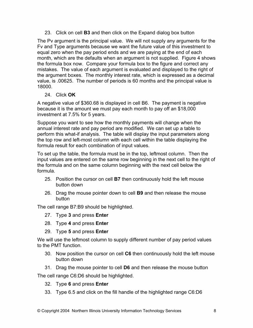
34. Continuously holding down on the left mouse button, drag the fill handle to column K, until the number 10 appears, and release the mouse button

We allowed Excel to use the pattern of 0.5 percent increases to set up a list of interest rates from six to ten in 0.5 increments. Now we can use row six to supply these different interest rate values to the PMT function. Figure PT-03 shows the column and row input values for this table along with the function. To set up the What-if table showing what payments would be across this range of payment periods and interest rates:

35. Position the cursor on cell B6 and hold the left mouse button down

36. Drag the mouse pointer to cell K9 and release the mouse button The cell range B6:K9 should be highlighted and if is not then repeat steps 35 and 36 above. You must highlight the entire cell range that will display the results of the table and the formula must be in the top, leftmost cell of the table.

37. Click on Data in the dropdown menus 38. Click on Table

A dialog box entitled Table appears with two options labeled Row input cell and Column input cell. We must specify the cell range containing the row input values within the table and the cell range containing the column input values.

39. Click within the box labeled Row input cell 40. Click on the Contract button 41. Click on cell B1

The cell address $B$1 should be filled into the Row input cell box. Cell B1 contains the annual interest rate and the table will replace the interest rate using the five values entered in cells C6, D6, E6, F6, and G6.

42. Click on the Expand button to return to the Table dialog box 43. Click within the Column input cell box 44. Click on the Contract button 45. Click on cell B2

Figure PT-03


The cell address $B$2 is filled into the Column input cell box. Cell B2 contains the number of periods and Excel will use the values supplied in cells B7, B8, and B9 to for the number of periods.

46. Click on the Expand button to return to the Table dialog box 47. Click on the OK button

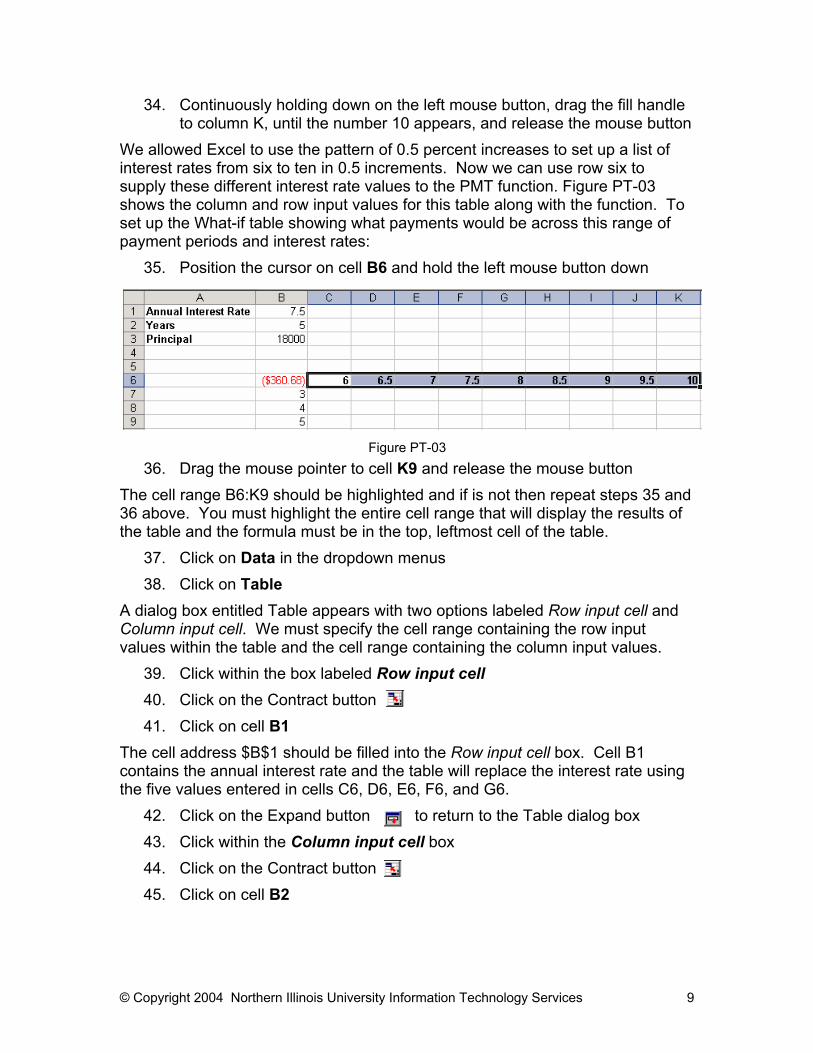
The table should result like Figure PT-04. Cell F9 displays the result of the PMT function using an annual interest rate of 7.5% and a pay period of 5 years.

This is the same result as cell B6 because these were the original values supplied to the function. Now you can compare the different payment values across different interest rates and pay periods. For example, cell E7 shows the monthly payment amount if the interest rate is 7% and the pay period is only 3 years. Cell G8 shows the monthly payment amount if the interest rate is 8% and the pay period is 4 years. The formatting of the monthly payments in the newly created table can be easily set using the Format Painter.

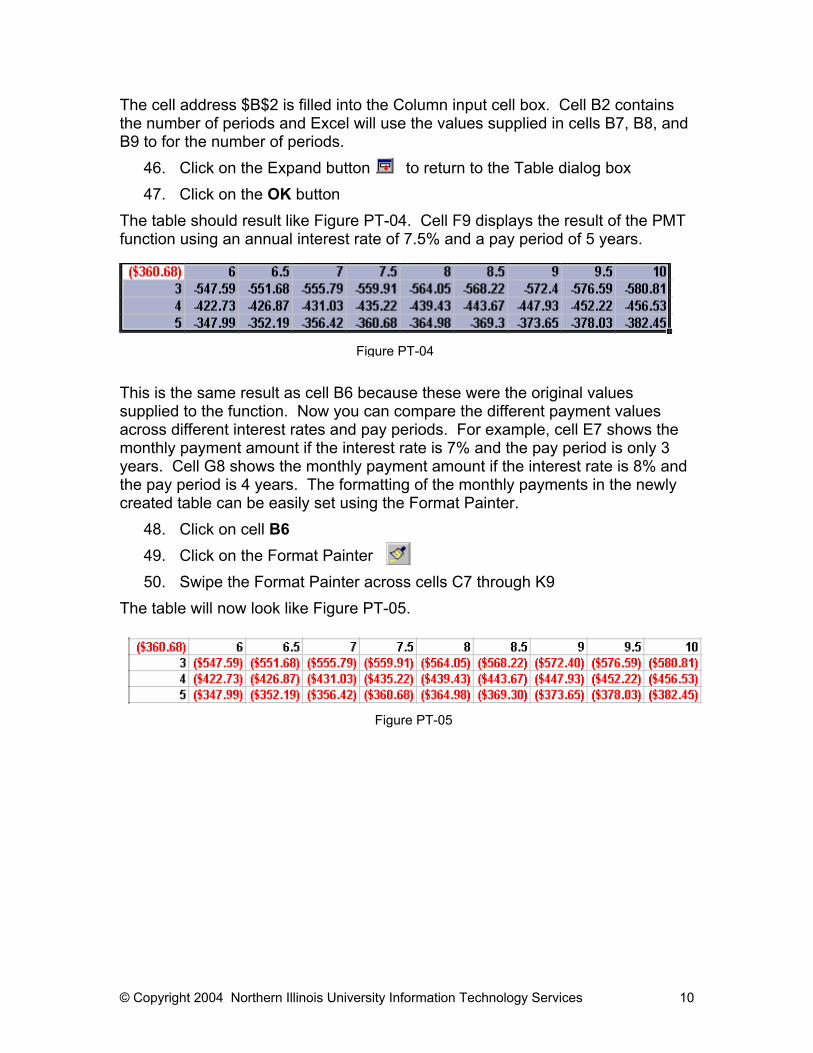
48. Click on cell B6 49. Click on the Format Painter 50. Swipe the Format Painter across cells C7 through K9

The table will now look like Figure PT-05.

Figure PT-04

Figure PT-05


Evaluating Trends Excel has a number of tools to assist in analyzing trends in data. Trend analysis can be utilized to predict future results. In this section we will use Excel’s Trendline tool to analyze several possible trends in a department’s tuition income. We will then utilize Excel’s Linear and Growth Trend tools to predict future tuition income based upon past results.

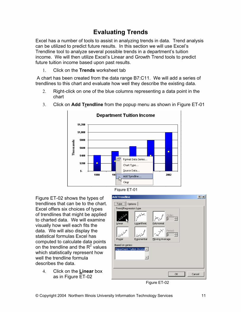
1. Click on the Trends worksheet tab A chart has been created from the data range B7:C11. We will add a series of trendlines to this chart and evaluate how well they describe the existing data.

2. Right-click on one of the blue columns representing a data point in the chart

3. Click on Add Trendline from the popup menu as shown in Figure ET-01 Figure ET-02 shows the types of trendlines that can be to the chart. Excel offers six choices of types of trendlines that might be applied to charted data. We will examine visually how well each fits the data. We will also display the statistical formulas Excel has computed to calculate data points on the trendline and the R2 values which statistically represent how well the trendline formula describes the data.

4. Click on the Linear box as in Figure ET-02

Figure ET-01

Figure ET-02


Figure TL6

5. Click OK A linear trendline has been applied to the chart.

6. Right-click on the trendline. The menu that pops up will allow you to either Format trendline or Clear the trendline

7. Click on Format Trendline The Format Trendline window that pops up has three tabs. The first, Patterns, will allow you to change the line style, color and weight of the trendline. The second, Type, will allow you to change the type of trendline being established.

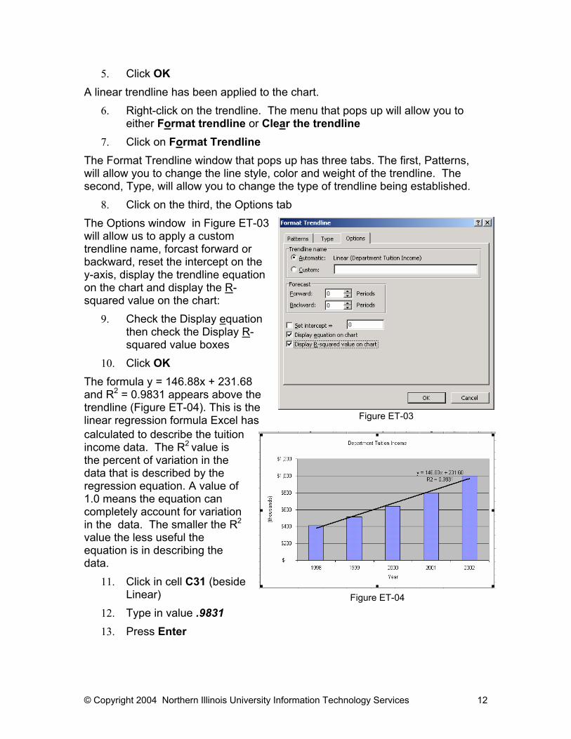
8. Click on the third, the Options tab The Options window in Figure ET-03 will allow us to apply a custom trendline name, forcast forward or backward, reset the intercept on the y-axis, display the trendline equation on the chart and display the R-squared value on the chart:

9. Check the Display equation then check the Display R-squared value boxes

10. Click OK The formula y = 146.88x + 231.68 and R2 = 0.9831 appears above the trendline (Figure ET-04). This is the linear regression formula Excel has calculated to describe the tuition income data. The R2 value is the percent of variation in the data that is described by the regression equation. A value of 1.0 means the equation can completely account for variation in the data. The smaller the R2

value the less useful the equation is in describing the data.

11. Click in cell C31 (beside Linear)

12. Type in value .9831 13. Press Enter

Figure ET-04

Figure ET-03


Since it is so easy to allow Excel to compute various types of regression equations we will proceed to look at each of the various types of equations and enter their R2 values beside the Trendline Type name in the table in cells B31 to C36.

14. Right-click on the trendline. 15. Click on the Type tab 16. Choose the next Trendline Type 17. Click OK 18. Click in the cell in column C corresponding to the trendline type and

enter the R2 value 19. Repeat steps 28 through 32 until R2 values for all trendline types have

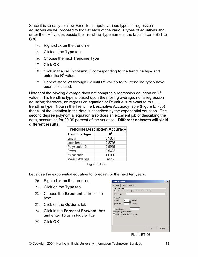
been calculated. Note that the Moving Average does not compute a regression equation or R2

value. This trendline type is based upon the moving average, not a regression equation; therefore, no regression equation or R2 value is relevant to this trendline type. Note in the Trendline Descriptive Accuracy table (Figure ET-05) that all of the variation in the data is described by the exponential equation. The second degree polynomial equation also does an excellent job of describing the data, accounting for 99.99 percent of the variation. Different datasets will yield different results.

Let’s use the exponential equation to forecast for the next ten years. 20. Right-click on the trendline. 21. Click on the Type tab 22. Choose the Exponential trendline

type 23. Click on the Options tab 24. Click in the Forecast Forward: box

and enter 10 as in Figure TL9 25. Click OK

Figure ET-05

Figure ET-06


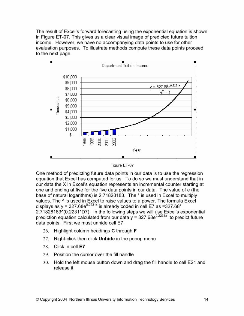
The result of Excel’s forward forecasting using the exponential equation is shown in Figure ET-07. This gives us a clear visual image of predicted future tuition income. However, we have no accompanying data points to use for other evaluation purposes. To illustrate methods compute these data points proceed to the next page.

One method of predicting future data points in our data is to use the regression equation that Excel has computed for us. To do so we must understand that in our data the X in Excel’s equation represents an incremental counter starting at one and ending at five for the five data points in our data. The value of e (the base of natural logarithms) is 2.71828183. The * is used in Excel to multiply values. The ^ is used in Excel to raise values to a power. The formula Excel displays as y = 327.68e0.2231x is already coded in cell E7 as =327.68* 2.71828183^(0.2231*D7). In the following steps we will use Excel’s exponential prediction equation calculated from our data y = 327.68e0.2231x to predict future data points. First we must unhide cell E7.

26. Highlight column headings C through F 27. Right-click then click Unhide in the popup menu 28. Click in cell E7 29. Position the cursor over the fill handle 30. Hold the left mouse button down and drag the fill handle to cell E21 and

release it

Figure ET-07


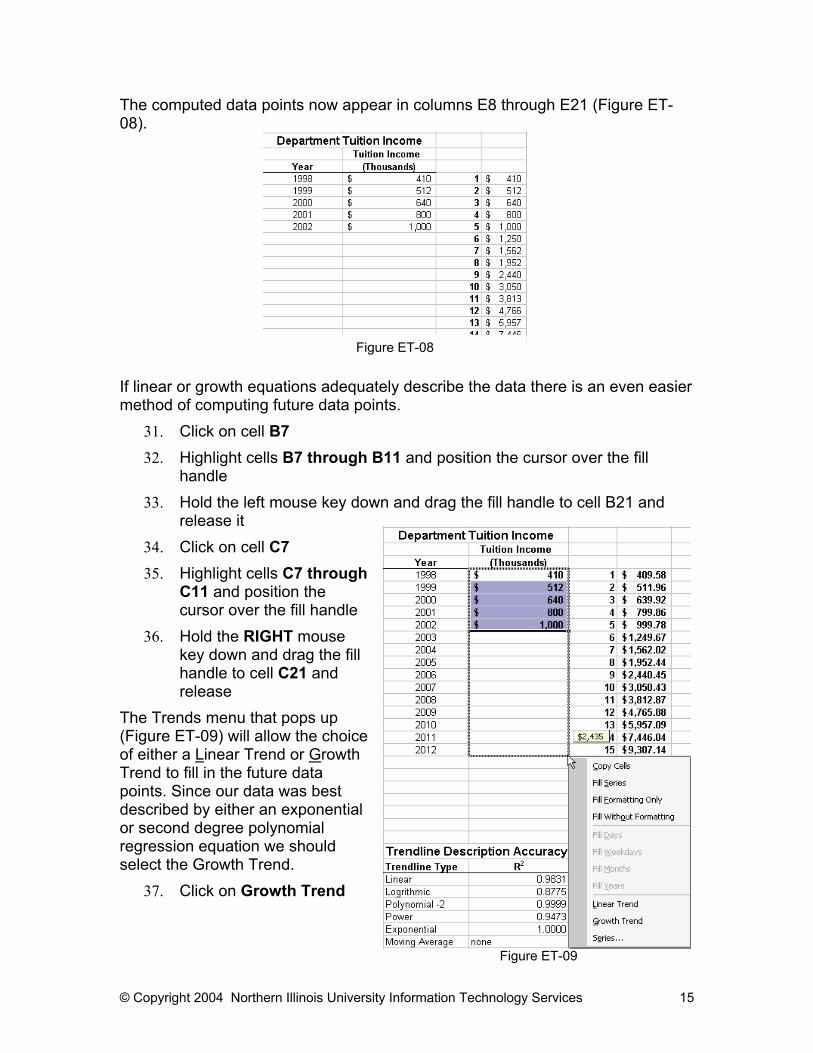
The computed data points now appear in columns E8 through E21 (Figure ET-08). If linear or growth equations adequately describe the data there is an even easier method of computing future data points.

31. Click on cell B7 32. Highlight cells B7 through B11 and position the cursor over the fill

handle 33. Hold the left mouse key down and drag the fill handle to cell B21 and

release it 34. Click on cell C7 35. Highlight cells C7 through

C11 and position the cursor over the fill handle

36. Hold the RIGHT mouse key down and drag the fill handle to cell C21 and release

The Trends menu that pops up (Figure ET-09) will allow the choice of either a Linear Trend or Growth Trend to fill in the future data points. Since our data was best described by either an exponential or second degree polynomial regression equation we should select the Growth Trend.

37. Click on Growth Trend

Figure ET-08

Figure ET-09


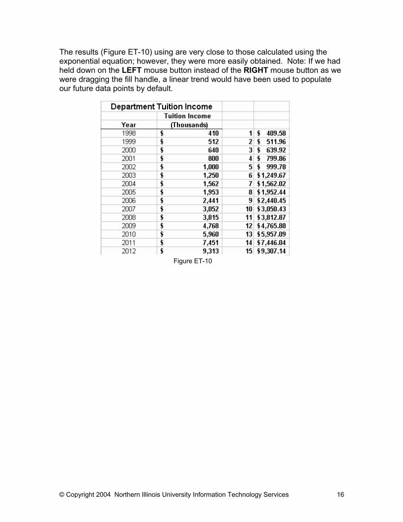
The results (Figure ET-10) using are very close to those calculated using the exponential equation; however, they were more easily obtained. Note: If we had held down on the LEFT mouse button instead of the RIGHT mouse button as we were dragging the fill handle, a linear trend would have been used to populate our future data points by default.

Figure ET-10


Using Goal Seek Goal Seek is one of Excel’s what-if tools. Goal Seek allows you to

• Specify a single adjustable cell.

• Specify a target value that is dependent upon the adjustable cell.

• Generate a solution by manipulating the value of the adjustable cell.

• Generate a single solution to a problem Goal Seek is a relatively easy tool to learn how to use and is a useful tool for finding solutions to complex problems involving a single variable. We will use it to find the coefficient required to reach a Department’s goals for growth in tuition income over the next ten years. The objective is to predict the coefficient of growth (x) required to achieve a ten-year goal and compute the annual tuition targets leading to that objective. It is assumed that the department has $1,000,000 of tuition income in the current year and that tuition income for each future year will increase by (x) times the previous year’s tuition total. This data and accompanying chart are present in the Goal Seek worksheet.

1. Click on the Goal Seek worksheet tab We want use the Goal Seek tool to compute the growth rate required to reach a goal of $10,000,000 of tuition income in the department by year 2011. The current tuition income in 2002 is $1,000,000. Over the past five years an annual growth rate of 125% has been achieved. Using this growth rate the tuition levels over the next ten years has been predicted in the table in the worksheet and charted in the accompanying chart. Tuition has been coded to thousands of dollars. This predicts the department will fail to reach the $10,000,000 tuition income target in 2011. We will use Goal Seek to determine what the future growth rate must be to reach the 2011 objective.

2. Click on cell C17. This is the location of our objective.

3. Click on Tools in the dropdown menus 4. Choose and click on Goal Seek

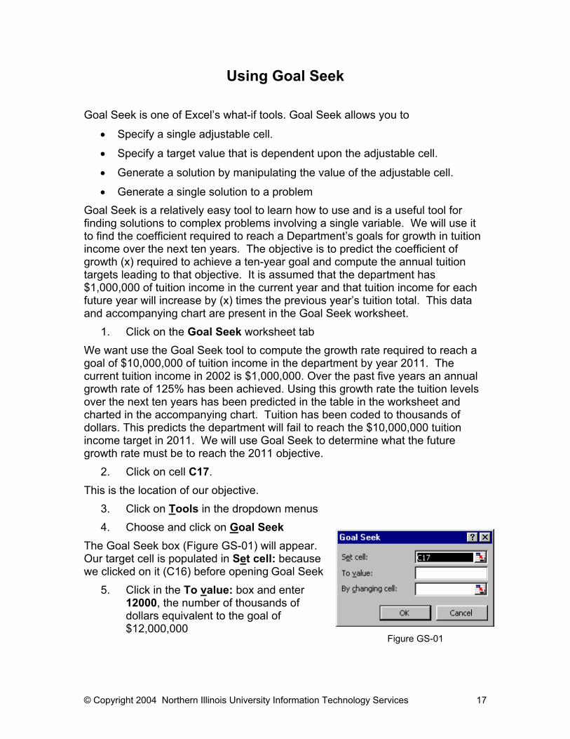
The Goal Seek box (Figure GS-01) will appear. Our target cell is populated in Set cell: because we clicked on it (C16) before opening Goal Seek

5. Click in the To value: box and enter 12000, the number of thousands of dollars equivalent to the goal of $12,000,000

Figure GS-01


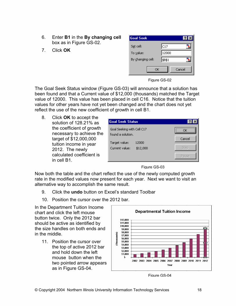
6. Enter B1 in the By changing cell box as in Figure GS-02.

7. Click OK The Goal Seek Status window (Figure GS-03) will announce that a solution has been found and that a Current value of $12,000 (thousands) matched the Target value of 12000. This value has been placed in cell C16. Notice that the tuition values for other years have not yet been changed and the chart does not yet reflect the use of the new coefficient of growth in cell B1.

8. Click OK to accept the solution of 128.21% as the coefficient of growth necessary to achieve the target of $12,000,000 tuition income in year 2012. The newly calculated coefficient is in cell B1.

Now both the table and the chart reflect the use of the newly computed growth rate in the modified values now present for each year. Next we want to visit an alternative way to accomplish the same result.

9. Click the undo button on Excel’s standard Toolbar 10. Position the cursor over the 2012 bar.

In the Department Tuition Income chart and click the left mouse button twice. Only the 2012 bar should be active as identified by the size handles on both ends and in the middle.

11. Position the cursor over the top of active 2012 bar and hold down the left mouse button when the two pointed arrow appears as in Figure GS-04.

Figure GS-02

Figure GS-03

Figure GS-04


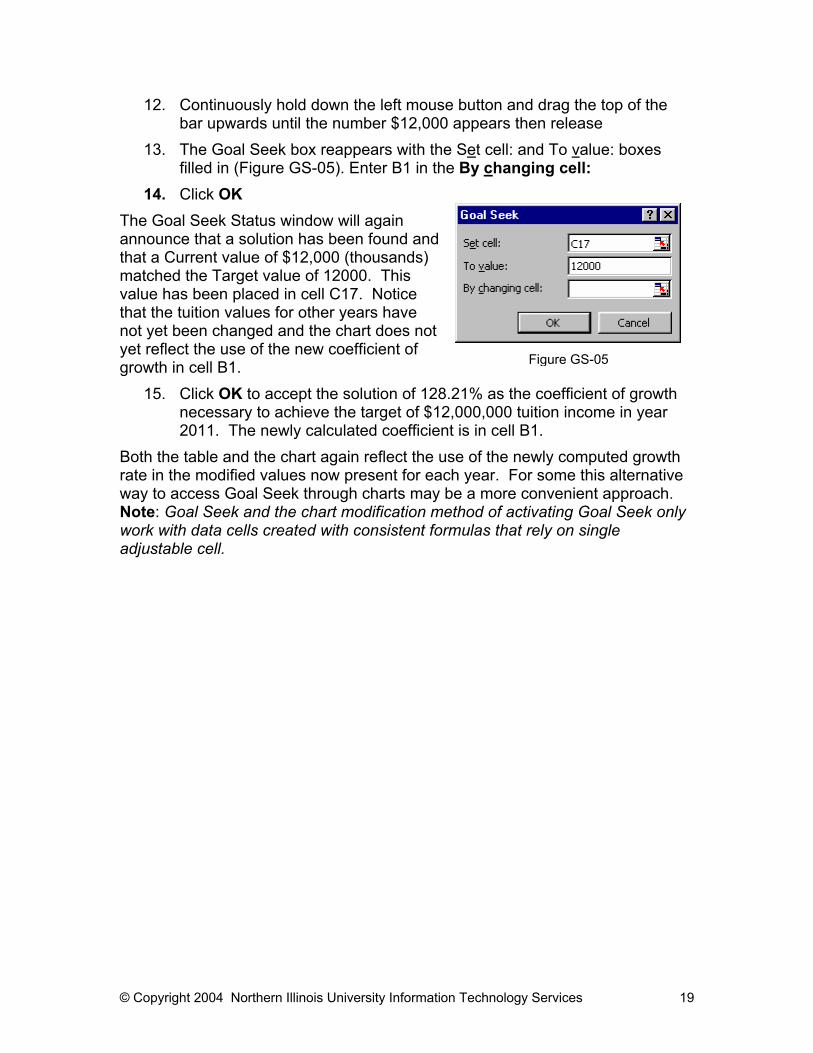
12. Continuously hold down the left mouse button and drag the top of the bar upwards until the number $12,000 appears then release

13. The Goal Seek box reappears with the Set cell: and To value: boxes filled in (Figure GS-05). Enter B1 in the By changing cell:

14. Click OK The Goal Seek Status window will again announce that a solution has been found and that a Current value of $12,000 (thousands) matched the Target value of 12000. This value has been placed in cell C17. Notice that the tuition values for other years have not yet been changed and the chart does not yet reflect the use of the new coefficient of growth in cell B1.

15. Click OK to accept the solution of 128.21% as the coefficient of growth necessary to achieve the target of $12,000,000 tuition income in year 2011. The newly calculated coefficient is in cell B1.

Both the table and the chart again reflect the use of the newly computed growth rate in the modified values now present for each year. For some this alternative way to access Goal Seek through charts may be a more convenient approach. Note: Goal Seek and the chart modification method of activating Goal Seek only work with data cells created with consistent formulas that rely on single adjustable cell.

Figure GS-05


Using Solver Solver is one of Excel’s add-in tools that allows you to

• Specify multiple adjustable cells.

• Specify constraints on the values that the adjustable cells can have.

• Generate a solution that maximizes or minimizes a particular worksheet cell.

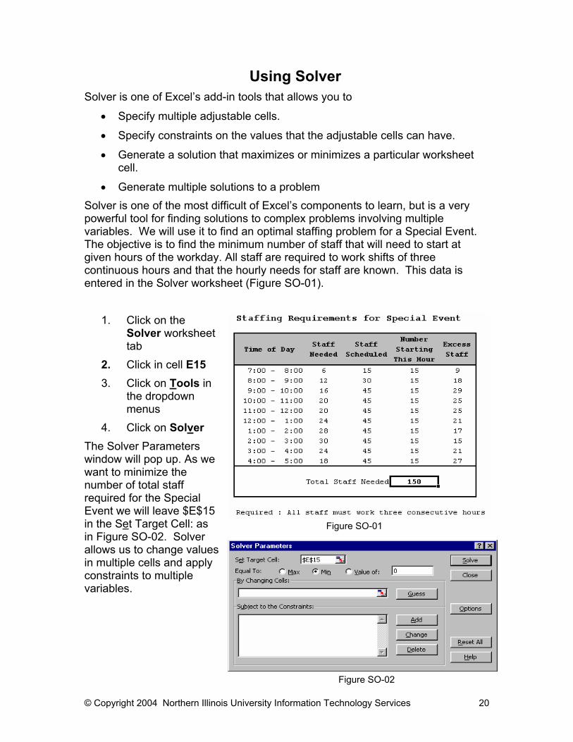
• Generate multiple solutions to a problem Solver is one of the most difficult of Excel’s components to learn, but is a very powerful tool for finding solutions to complex problems involving multiple variables. We will use it to find an optimal staffing problem for a Special Event. The objective is to find the minimum number of staff that will need to start at given hours of the workday. All staff are required to work shifts of three continuous hours and that the hourly needs for staff are known. This data is entered in the Solver worksheet (Figure SO-01).

1. Click on the Solver worksheet tab

2. Click in cell E15 3. Click on Tools in

the dropdown menus

4. Click on Solver The Solver Parameters window will pop up. As we want to minimize the number of total staff required for the Special Event we will leave $E$15 in the Set Target Cell: as in Figure SO-02. Solver allows us to change values in multiple cells and apply constraints to multiple variables.

Figure SO-02

Figure SO-01


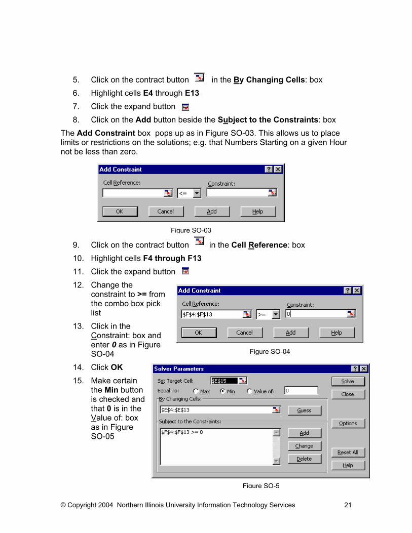
5. Click on the contract button in the By Changing Cells: box 6. Highlight cells E4 through E13 7. Click the expand button 8. Click on the Add button beside the Subject to the Constraints: box

The Add Constraint box pops up as in Figure SO-03. This allows us to place limits or restrictions on the solutions; e.g. that Numbers Starting on a given Hour not be less than zero.

9. Click on the contract button in the Cell Reference: box 10. Highlight cells F4 through F13 11. Click the expand button 12. Change the

constraint to >= from the combo box pick list

13. Click in the Constraint: box and enter 0 as in Figure SO-04

14. Click OK 15. Make certain

the Min button is checked and that 0 is in the Value of: box as in Figure SO-05

Figure SO-03

Figure SO-04

Figure SO-5


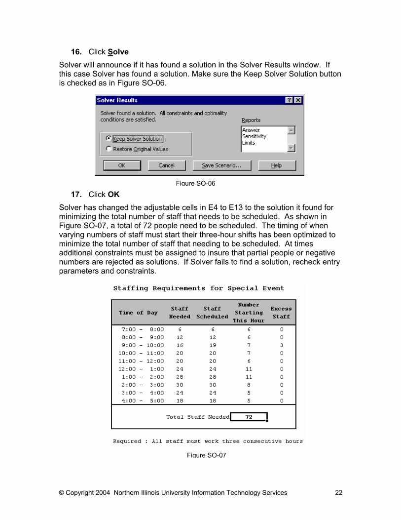
16. Click Solve Solver will announce if it has found a solution in the Solver Results window. If this case Solver has found a solution. Make sure the Keep Solver Solution button is checked as in Figure SO-06.

17. Click OK Solver has changed the adjustable cells in E4 to E13 to the solution it found for minimizing the total number of staff that needs to be scheduled. As shown in Figure SO-07, a total of 72 people need to be scheduled. The timing of when varying numbers of staff must start their three-hour shifts has been optimized to minimize the total number of staff that needing to be scheduled. At times additional constraints must be assigned to insure that partial people or negative numbers are rejected as solutions. If Solver fails to find a solution, recheck entry parameters and constraints.

Figure SO-06

Figure SO7

Figure SO-07


Creating Scenarios

Scenarios are a tool Excel has to allow us to look and be able to recall the effects of making multiple changes to cells affecting the results of our worksheet. Excel's Scenario Manager feature makes it easy to automate your what-if models. You can store different sets of input values (called changing cells by Scenario Manager) for any number of variables and give a name to each set. You can then select a set of values by name, and Excel displays the worksheet by using those values. Next we will try out the Scenario Manager.

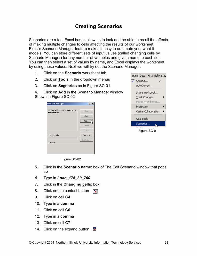
1. Click on the Scenario worksheet tab 2. Click on Tools in the dropdown menus 3. Click on Scenarios as in Figure SC-01 4. Click on Add in the Scenario Manager window Shown in Figure SC-02

5. Click in the Scenario name: box of The Edit Scenario window that pops up

6. Type in Loan_175_30_700 7. Click in the Changing cells: box 8. Click on the contact button 9. Click on cell C4 10. Type in a comma 11. Click on cell C6 12. Type in a comma 13. Click on cell C7 14. Click on the expand button

Figure SC-01

Figure SC-02


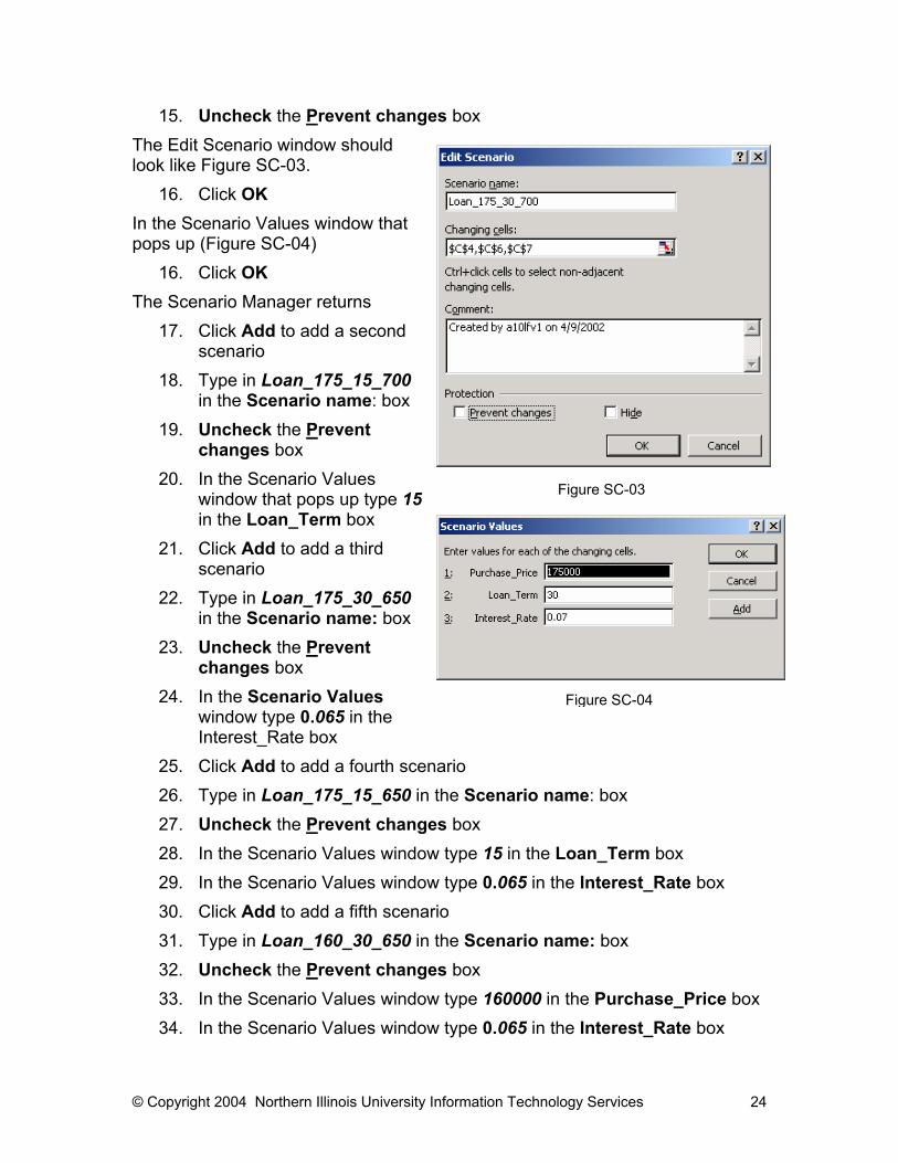
15. Uncheck the Prevent changes box The Edit Scenario window should look like Figure SC-03.

16. Click OK In the Scenario Values window that pops up (Figure SC-04)

16. Click OK The Scenario Manager returns

17. Click Add to add a second scenario

18. Type in Loan_175_15_700 in the Scenario name: box

19. Uncheck the Prevent changes box

20. In the Scenario Values window that pops up type 15 in the Loan_Term box

21. Click Add to add a third scenario

22. Type in Loan_175_30_650 in the Scenario name: box

23. Uncheck the Prevent changes box

24. In the Scenario Values window type 0.065 in the Interest_Rate box

25. Click Add to add a fourth scenario 26. Type in Loan_175_15_650 in the Scenario name: box 27. Uncheck the Prevent changes box 28. In the Scenario Values window type 15 in the Loan_Term box 29. In the Scenario Values window type 0.065 in the Interest_Rate box 30. Click Add to add a fifth scenario 31. Type in Loan_160_30_650 in the Scenario name: box 32. Uncheck the Prevent changes box 33. In the Scenario Values window type 160000 in the Purchase_Price box 34. In the Scenario Values window type 0.065 in the Interest_Rate box

Figure SC-03

Figure SC-04


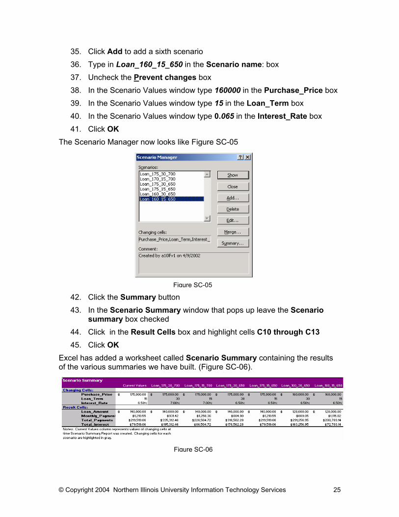
35. Click Add to add a sixth scenario 36. Type in Loan_160_15_650 in the Scenario name: box 37. Uncheck the Prevent changes box 38. In the Scenario Values window type 160000 in the Purchase_Price box 39. In the Scenario Values window type 15 in the Loan_Term box 40. In the Scenario Values window type 0.065 in the Interest_Rate box 41. Click OK

The Scenario Manager now looks like Figure SC-05

42. Click the Summary button 43. In the Scenario Summary window that pops up leave the Scenario

summary box checked 44. Click in the Result Cells box and highlight cells C10 through C13 45. Click OK

Excel has added a worksheet called Scenario Summary containing the results of the various summaries we have built. (Figure SC-06).

Figure SC-05

Figure SC-06

Documents

Microsoft Excel 2003 - Department of Psychology ... · Microsoft Excel 2003 Data Analysis ... Using Excel’s Data Analysis Tools Excel includes a number of add-in tools to assist