Embed Size (px)
Citation preview
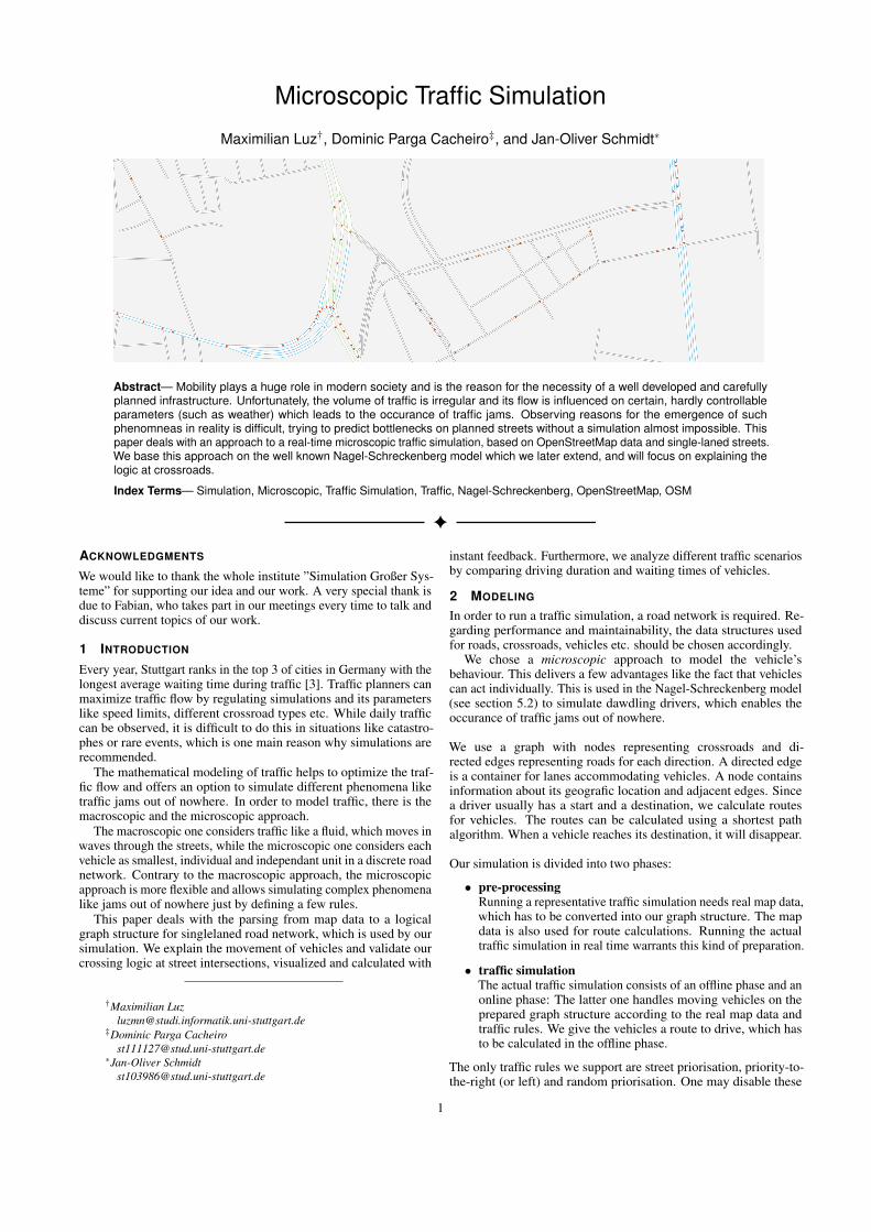
Microscopic Traffic Simulation
Maximilian Luz†, Dominic Parga Cacheiro‡, and Jan-Oliver Schmidt∗
Abstract— Mobility plays a huge role in modern society and is the reason for the necessity of a well developed and carefullyplanned infrastructure. Unfortunately, the volume of traffic is irregular and its flow is influenced on certain, hardly controllableparameters (such as weather) which leads to the occurance of traffic jams. Observing reasons for the emergence of suchphenomneas in reality is difficult, trying to predict bottlenecks on planned streets without a simulation almost impossible. Thispaper deals with an approach to a real-time microscopic traffic simulation, based on OpenStreetMap data and single-laned streets.We base this approach on the well known Nagel-Schreckenberg model which we later extend, and will focus on explaining thelogic at crossroads.
Index Terms— Simulation, Microscopic, Traffic Simulation, Traffic, Nagel-Schreckenberg, OpenStreetMap, OSM
ACKNOWLEDGMENTS
We would like to thank the whole institute ”Simulation Großer Sys-teme” for supporting our idea and our work. A very special thank isdue to Fabian, who takes part in our meetings every time to talk anddiscuss current topics of our work.
1 INTRODUCTION
Every year, Stuttgart ranks in the top 3 of cities in Germany with thelongest average waiting time during traffic [3]. Traffic planners canmaximize traffic flow by regulating simulations and its parameterslike speed limits, different crossroad types etc. While daily trafficcan be observed, it is difficult to do this in situations like catastro-phes or rare events, which is one main reason why simulations arerecommended.
The mathematical modeling of traffic helps to optimize the traf-fic flow and offers an option to simulate different phenomena liketraffic jams out of nowhere. In order to model traffic, there is themacroscopic and the microscopic approach.
The macroscopic one considers traffic like a fluid, which moves inwaves through the streets, while the microscopic one considers eachvehicle as smallest, individual and independant unit in a discrete roadnetwork. Contrary to the macroscopic approach, the microscopicapproach is more flexible and allows simulating complex phenomenalike jams out of nowhere just by defining a few rules.
This paper deals with the parsing from map data to a logicalgraph structure for singlelaned road network, which is used by oursimulation. We explain the movement of vehicles and validate ourcrossing logic at street intersections, visualized and calculated with
†Maximilian [email protected]
‡Dominic Parga [email protected]
∗Jan-Oliver [email protected]
instant feedback. Furthermore, we analyze different traffic scenariosby comparing driving duration and waiting times of vehicles.
2 MODELING
In order to run a traffic simulation, a road network is required. Re-garding performance and maintainability, the data structures usedfor roads, crossroads, vehicles etc. should be chosen accordingly.
We chose a microscopic approach to model the vehicle’sbehaviour. This delivers a few advantages like the fact that vehiclescan act individually. This is used in the Nagel-Schreckenberg model(see section 5.2) to simulate dawdling drivers, which enables theoccurance of traffic jams out of nowhere.
We use a graph with nodes representing crossroads and di-rected edges representing roads for each direction. A directed edgeis a container for lanes accommodating vehicles. A node containsinformation about its geografic location and adjacent edges. Sincea driver usually has a start and a destination, we calculate routesfor vehicles. The routes can be calculated using a shortest pathalgorithm. When a vehicle reaches its destination, it will disappear.
Our simulation is divided into two phases:
• pre-processingRunning a representative traffic simulation needs real map data,which has to be converted into our graph structure. The mapdata is also used for route calculations. Running the actualtraffic simulation in real time warrants this kind of preparation.
• traffic simulationThe actual traffic simulation consists of an offline phase and anonline phase: The latter one handles moving vehicles on theprepared graph structure according to the real map data andtraffic rules. We give the vehicles a route to drive, which hasto be calculated in the offline phase.
The only traffic rules we support are street priorisation, priority-to-the-right (or left) and random priorisation. One may disable these
1
rules seperately, too. Traffic lights are not supported yet.
3 PRE-PROCESSING
The primary objective of the pre-processing stage is to extract theabove discussed data from a given source and present it to thesimulation- and visualization-framework. The secondary objectiveis to do so in a way, that the following stages are able to operateefficiently and in real-time on large data sets, such as the admin-istrative district of Stuttgart (with over 250000 relevant streets inOpenStreetMap).
In this section, we will be discussing OpenStreetMap as a sourcefor this simulation, its implications on the pre-processing pipelineand finally give a detailed overview of said.
3.1 OpenStreetMapThe OpenStreetMap (OSM) project is a collaborative effort to pro-vide free geographic data for the whole world. Founded in 2004 [5],it has long since become a viable alternative to large, commercialproducts like Google Maps and can not only be used for creatingvisual maps for multiple aspects (public transport, cycling, emer-gency healthcare support, etc.) but also for other applications, forinstance, routing. OpenStreetMap provides a vast amount of fea-tures, including but not limited to many street properties, some ofwhich we will discuss later. This and the fact that it is freely andeasily accessible as well as editable has led to its widespread use ingeographic applications.
Being fully community driven, the provided data is constantlyimproving in both, accuracy and completeness. While it may notbe able to match the overall quality of geographic data provided byprofessional companies or government agencies such as the BritishOrdnance Survey, it is suitable for almost any use-case.
The actual data can be obtained in several formats, includingXML and Protocol Buffer based versions. Most available formatsfollow the same structure, however due to simplicity we will focuson the more popular XML variant. The described data is separatedinto three different primitive types: node, way and relation. Nodesdescribe a spatial position, ways a succession of nodes, and relationsa relation between any of these three primitives. In general, streetsare modeled as ways with certain properties. Intersections betweenstreets are represented as a shared node, complex intersections areoften expressed using multiple smaller intersections. To store ad-ditional information such as the previously mentioned properties,every primitive may contain several key-value-pairs, the so calledtags. Through these, OpenStreetMap provides all the necessary in-formation for this simulation. Using the highway-tag, we can detectand classify streets as well as give them logical priorities for thestreet-graph. For the scenarios below, the included types are: motor-way, trunk, primary, secondary, tertiary as well as their link-types,unclassified, residential, living-street, and road. There are severaladditional types, however, many of these may only be accessibleto certain vehicle-types or pedestrians. Furthermore, the provideddata not only contains the type of the street, but also the amountof lanes per direction (lanes-tag), the speed-limit (maxspeed-tag),the information whether a street is a one-way-street (oneway-tag)and several other tags currently not used by the simulation such astags for traffic-lights and signs. There are also several tags purelyfor rendering, such as the bridge- or tunnel-tags. However, not ev-ery property of a street can be expressed using tags. For example,turn-restrictions are modeled using relations which are themselvescategorized and expanded by tags.
The dynamic tag-based approach allows for flexibility and a sim-ple parser base implementation, but it also has several drawbacks.While most of the tags are described clearly in the OpenStreetMapwiki, some differences and inaccuracies may arise in the actual dataset, as it is community-based and every user has their own ideaof how things should be tagged. This problem gets worse whencodependent tags like the number of lanes per direction and theone-way information are inconsistent, although such things do notoccur often.
As seen above, OpenStreetMap is able to supply enough detailfor traffic simulation. Although it may not be able to provide thenecessary quality for highly professional applications, its availabilityand the large amount of existing tools (including editors and formatconverters) make it a viable alternative to commercial products, anda reasonable choice for this project.
3.2 Pre-Processing PipelineThe pre-processing pipeline consists of several stages includingparsing, sanitization, pre-processing for runtime-efficiency improve-ments and the actual generation of the desired data structures. Tonot extend the scope of this paper, we will only cover some moreimportant aspects in depth and outline others.
3.2.1 Intermediate Representation of Extracted Data
To keep the pre-processing pipeline flexible and extendable, we rep-resent the nodes and ways from OpenStreetMap using a modifiedentity-component system. Entity-component systems are a dynamicarchitectural pattern based on composition. Due to its flexibility, itis often used in game-development. Objects are modeled as entitieswhose behavior and data is defined through their attached compo-nents. Normally, entities do not contain any information itself otherthan a unique identifier and, depending on the implementation, alist of their components. Since we only have two general entitytypes, nodes and ways (relations are handled differently due to theirunique types), we also use them to store the basic information of theprimitives they represent. Components are used to store groups oftags describing the primitive concerning a common aspect, e.g. thesimulation parameters (highway, lanes, etc.). This allows to almostdirectly model OpenStreetMaps data representation and gives theflexibility to easily extend the pre-processing pipeline, for exampleto increase diversity of the visualization by simply adding a newcomponent-type and its parser module.
3.2.2 Parsing and Feature Sets
Parsing the OpenStreetMap data is the first step of the pipeline. Asmentioned earlier, implementing a base-parser for the XML-formatis quite simple and the required data can be filtered out easily usingpredicates on the primitives and their tags. However, ways andrelations depend on other primitives such as nodes, and in generalOpenStreetMap files contain much additional information we donot care about in our simulation. To include dependent primitiveswithout loading all nodes, ways and relations into memory, the parserruns multiple passes over the input file.
Additionally to extracting the intermediate format, the parsercategorizes the created entities by assigning them to feature sets,again using predicates based on tags. These feature sets describehow the contained entities are used later in the simulation and/orvisualization. For example, one feature set may contain all relevantstreets used in the simulation, while a second one contains all streetsof major-, and a third all streets of minor type. In this example thesecond and third feature set are used purely for visualization. Notethat a single entity may be assigned to multiple feature sets. Basedon the assigned feature sets, the pre-processing pipeline is later ableto determine which data structures should be generated and whatthey contain. In context of visualization, this approach also allowsthe creation of layers based on feature sets (see figure 1).
3.2.3 Sanitization
Except for filtering, categorizing and evaluating strong implications(e.g. oneway = ungiven∧ oneway 6= motorway→ oneway = no),the parser directly extracts the given OpenStreetMap data to theintermediate representation. As described previously, this data maycontain inconsistencies; the sanitization step aims to eliminate these.Furthermore, some required properties may be unspecified or containvalues unsupported by the simulation (e.g. maxspeed=signals – thesimulation cannot handle speed-limits imposed by dynamic signalssuch as electronic signs) and thus have to be set correctly.
2
An issue affecting the simulation, which cannot be handled in thisstep (without introducing additional complexity), is double geometry,respectively double streets. We approach this problem in the street-processing step.
3.2.4 Pre-Processing Streets
In OpenStreetMap, streets are modeled by a succession of nodes,where a node shared between two or more streets represents a cross-ing. A junction-node may not only be the first or last, but any nodeof this sequence, furthermore a street may intersect itself. A naıveapproach to generate a graph representation of this street-networkwould be to simply model each connection between two nodes as anedge. This, however, has two flaws. Both of them are based on thefact that, using the naıve approach, a street with a complex coursecontaining numerous nodes will be divided into many graph-nodesand edges. The first flaw is, that each edge of the final graph isdivided into a discrete number of cells, depending on the length ofthe represented street segment. Creating many small edges insteadof fewer but larger ones increases the error introduced by roundingthe segment length, even more so considering that an edge mustcontain at least one cell. The second and more important flaw is,that each graph-node is interpreted as a crossroad. This meansthat using the naıve approach would introduce a large amount ofsimple two-street-connections (end to end) that are unnecessarilyinterpreted as crossings, and thus have a major negative influence onthe runtime-performance.
One solution to this problem is – in theory and for an undirectedgraph – simple: Generate a minimal graph by removing nodes withonly two adjacent edges and merging these edges to keep the con-nectivity. In practice, we do not work on a graph to begin with, butthe OpenStreetMap street-network as described above. Additionally,the resulting graph is directed and the edges may have different prop-erties based on which they sometimes cannot be merged. Despitesaid complications this solution is still feasible and it can be dividedinto three major steps: apply restrictions, split and merge, a generaloutline is given as Algorithm 1.
Apply Restrictions Before we can bring the street-network intoa graph-friendly representation (using split and merge), we needto look at turn-restrictions. In OpenStreetMap, these restrictionsare modeled using relations between streets and nodes, and rela-tions reference their participants using unique IDs. The proposedsteps, however, will destroy the binding between street and ID, thusrelations concerning these streets have to be applied before. Tohandle restriction relations, we introduce street-connectors. Theseconnectors are triplets (from,via, to) and indicate an unrestrictedconnection from one street via a node to another street. For eachstreet we now store three sets of connectors: incoming, outgoingand u-turns. Changes to a street can easily be propagated ontothese sets, and during construction of the street-graph the requiredlane-connectors can be derived from these street-connectors.
Split The split-step splits each street on every inner node, sharedbetween at least two streets and therefore the resulting street-networkcontains crossroads only on start or end nodes of street-segments.Such a segment could now be directly mapped to one edge perstreet-direction of a valid street-graph.
Merge The merge-step ensures that the generated graph is mini-mal by – if possible – merging streets on crossroads with only twoparticipants. Note that due to incompatible street-connectors ordifferent properties, not every crossing between exactly two streetscan be removed. After this step, the street network can be easilyconverted to a minimal directed graph (see Algorithm 1).
Removing Double Streets Detecting and removing doublestreet segments can best be done between the split- and merge-step. Between these two steps, double street segments will haveexactly two nodes (double segments intersect on every node), makingcomparison simple.
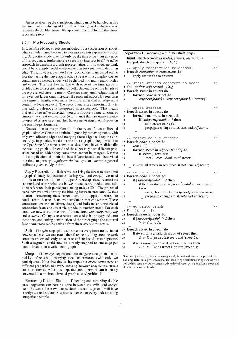
Algorithm 1: Generating a minimal street-graph.Input: street-network as nodes , streets , restrictionsOutput: directed graph G = (V,E)
/* apply restriction relations */1 foreach restriction in restrictions do2 apply restriction to streets;
/* store streets adjacent to nodes */3 ∀n ∈ nodes : adjacent[n] 7→ /0m;4 foreach street in streets do5 foreach node in street do6 adjacent[node]← adjacent[node]∪{street};
/* split streets */7 foreach street in streets do8 foreach inner node in street do9 if |adjacent[node]| ≥ 2 then
10 split street on node;11 propagate changes to streets and adjacent;
/* remove double streets */12 foreach node in nodes do13 rem←{};14 foreach street in adjacent[ node] do15 if street 6∈ rem then16 rem← rem∪doubles of street;
17 remove all streets in rem from streets and adjacent;
/* merge streets */18 foreach node in nodes do19 if |adjacent[node]|= 2 then20 if the two streets in adjacent[ node] are mergeable
then21 merge both streets in adjacent[ node] on node;22 propagate changes to streets and adjacent;
/* generate graph */23 V ←{}; E←{};24 foreach node in nodes do25 if |adjacent[node]| ≥ 2 then26 V ←V ∪node;
27 foreach street in streets do28 if forwards is a valid direction of street then29 E← E ∪ (start(street),end(street));
30 if backwards is a valid direction of street then31 E← E ∪ (end(street),start(street));
Notation: {} is used to denote an empty set, /0m is used to denote an empty multiset.For simplicity, this algorithm assumes that modifying a collection during iteration has awell defined semantic: Any changes made to the collection during iteration are executedafter the iteration has finished.
3

Figure 1: Illustration of the layer-based visualization approach.(https://wiki.openstreetmap.org/wiki/File:Layer-stack.jpg)
4 VISUALIZATION
For real-time simulations such as the one discussed in this paper,displaying live data is a key feature. While many observations canbe summarized during execution and visualized off-line, recordingand storing details often requires a large amount of memory. This is,in case of easily repeatable, deterministic1real-time simulations, notnecessary and makes live visualization the preferred method. How-ever, executing visualization and simulation in parallel puts stricterconstraints (e.g. memory, performance) on the said subsystem.
We will begin this section with an overview of the implementedvisualization subsystem, followed by a short introduction to mapprojections. Lastly, we will discuss two more technical aspects: Linerendering and vehicle visualization in context of OpenGL.
4.1 Overview of the SubsystemClassic online map visualizations, such as Google Maps or theOpenStreetMap web interface, use pre-rendered images, so calledimage-tiles. Tiles are the result of subdividing the map to be drawnat fixed zoom-levels into equally sized and axis aligned rectangularslices (usually creating a quad-tree with one tile per tree-node). Thebenefit of using pre-rendered tiles is a runtime-efficient visualization,however due to the considerable amount of memory2required forstoring these tiles, this approach is not feasible in our case. Analternative would be to utilize the OpenStreetMap tile-server, butthis would limit the visualization to a predefined style and worse, itwould disallow the use of custom generated or modified map files.
For our implementation we decided to use the Open GraphicsLibrary (OpenGL) version 3.3 and a strictly two-dimensional, tile-based approach, compositing the tiles on the fly as required. OpenGLallows for fast, hardware-based and platform independent renderingof basic primitives including triangles, lines and points. Similar tocommon map visualization methods, we generate layers by associat-ing the map-features described in Section 3.2.2 with customizablestyles and blending them together as illustrated in Figure 1. In ad-dition, we differentiate between layers of static and dynamic data:Static data is assumed to change infrequently or not at all, thusmaking it possible to create, maintain, and render via a tiled data
1 The presented simulation uses pseudo-random number generators, thusdeterminism can be achieved by initializing them with known seeds.
2 Assuming a quad-tree based tiling scheme and approximately 633 Bper tile [5], the required memory would be m≈ 633B ·∑n
i=0 22i. For a zoom-level difference (full zoom minus the zoom level on which the completemap-segment can be displayed in one tile) of n = 10, this results in m ≈844MiB, with a zoom-level difference of n = 15 already in m≈ 844GiB ofpre-rendered imagery. A real world example, using OpenStreetMap: Thedistrict of Tokyo can fit on one tile at zoom-level 7. With a maximum zoomlevel of 19, it would require approximately 13.2 GiB.
structure. Dynamic data is assumed to change every frame, thereforea tiled data structure cannot be maintained efficiently. We displaydynamic data (such as the simulated vehicles) directly, atop of thestatic tiles.
4.2 ProjectionsOpenStreetMap uses the WGS 84 coordinate reference system (alsoknown as EPSG:4326) to provide its geographic information [5].This system is based on a spheroid, coordinates are given in latitude(−90◦ to 90◦, south to north) and longitude (−180◦ to 180◦, west toeast). It is mainly used by the Global Positioning System (GPS) andvery suitable for the task of providing accurate geospatial data, how-ever, projections are required to transform the spherical coordinatesinto a two dimensional, visualization friendly, planar representation.
One of the most simplistic projections is the equidistant cylindri-cal (also referred to as equirectangular) projection. This projectionis achieved by replacing the spheroid with a cylinder defining itsheight as latitude, and then unrolling it. The radius of this cylinderdefines the standard parallel, i.e. the latitude at which the scale of theprojection is one. Using the equator as the standard parallel (ϕ1 = 0in Equations 1) yields the Plate Carree projection. In formulas, thisprojection can be written as (omitting terms of east-west adjustmentand scaling)
x = λ cosϕ1y = ϕ
(1)
with λ as longitude, ϕ as latitude, and ϕ1 as standard parallel [6].Besides its simplicity, an important aspect of this projection is thatmeridians and parallels are equidistant straight lines, intersectingat right angles [6]. A major problem with this projection is thedistortion: The scale in x-direction is dependent on the latitude,while the scale on the y-axis is constant.
The Mercator projection fixes said scale problems while keepingthe equidistant and orthogonal properties of meridians and parallels:The scale changes uniformly in x- and y-direction, depending on thelatitude. Different variations of this projection (e.g. Web-Mercator)are often used for map visualization such as OpenStreetMap andGoogle Maps. In formulas, the Mercator projection can be writtenas
x = λ
y = ln tan(
π
4 + ϕ
2) (2)
(again omitting terms of east-west adjustment and scaling) [6]. Bylimiting y to [−π,π] (and thus ϕ to approx [−85◦,85◦]) the resultingrectangular plane can be turned into a square making it ideal for tilebased rendering.
4.3 Technical AspectsIn the following paragraphs we will briefly discuss a few technicalaspects, mainly addressing performance. Please note that this isnot a computer graphics paper, thus implementation details will beomitted.
4.3.1 Drawing Lines in OpenGLThe line rendering capabilities of OpenGL are, to say the least, lim-ited. OpenGL does neither support joins nor caps, and the availablevalues for the line width (other than one pixel) are implementationdependent. Lines may be drawn anti-aliased, but when doing so, theline width may be restricted even more. However one has to keep inmind that OpenGL is designed for performance, providing a smallset of functions around a flexible rendering pipeline, and is not alarge abstract drawing library.
To display lines realiably, we have to transform them into a trian-gle mesh as shown in Figure 2. Anti-aliasing can be achieved using asigned distance vector and exploiting the parameter interpolation onfragments between vertices: The length of distance vector indicatesthe distance from a fragment to the center of the line, based on whichthe OpenGL smoothstep function (Hermite interpolation) can beapplied to the alpha value. This generates a smooth transition of thealpha value between zero and one in a definable radius.
4
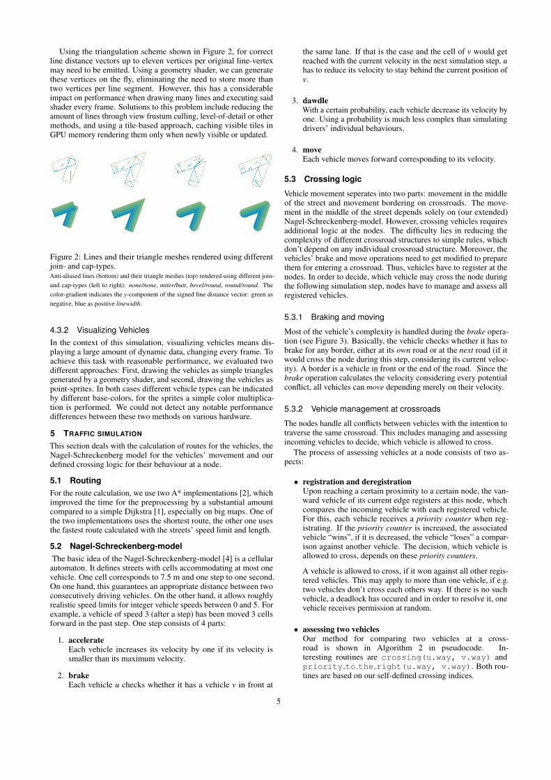
Using the triangulation scheme shown in Figure 2, for correctline distance vectors up to eleven vertices per original line-vertexmay need to be emitted. Using a geometry shader, we can generatethese vertices on the fly, eliminating the need to store more thantwo vertices per line segment. However, this has a considerableimpact on performance when drawing many lines and executing saidshader every frame. Solutions to this problem include reducing theamount of lines through view frustum culling, level-of-detail or othermethods, and using a tile-based approach, caching visible tiles inGPU memory rendering them only when newly visible or updated.
Figure 2: Lines and their triangle meshes rendered using differentjoin- and cap-types.Anti-aliased lines (bottom) and their triangle meshes (top) rendered using different join-and cap-types (left to right): none/none, miter/butt, bevel/round, round/round. Thecolor-gradient indicates the y-component of the signed line distance vector: green asnegative, blue as positive linewidth.
4.3.2 Visualizing VehiclesIn the context of this simulation, visualizing vehicles means dis-playing a large amount of dynamic data, changing every frame. Toachieve this task with reasonable performance, we evaluated twodifferent approaches: First, drawing the vehicles as simple trianglesgenerated by a geometry shader, and second, drawing the vehicles aspoint-sprites. In both cases different vehicle types can be indicatedby different base-colors, for the sprites a simple color multiplica-tion is performed. We could not detect any notable performancedifferences between these two methods on various hardware.
5 TRAFFIC SIMULATION
This section deals with the calculation of routes for the vehicles, theNagel-Schreckenberg model for the vehicles’ movement and ourdefined crossing logic for their behaviour at a node.
5.1 RoutingFor the route calculation, we use two A* implementations [2], whichimproved the time for the preprocessing by a substantial amountcompared to a simple Dijkstra [1], especially on big maps. One ofthe two implementations uses the shortest route, the other one usesthe fastest route calculated with the streets’ speed limit and length.
5.2 Nagel-Schreckenberg-modelThe basic idea of the Nagel-Schreckenberg-model [4] is a cellular
automaton. It defines streets with cells accommodating at most onevehicle. One cell corresponds to 7.5 m and one step to one second.On one hand, this guarantees an appropriate distance between twoconsecutively driving vehicles. On the other hand, it allows roughlyrealistic speed limits for integer vehicle speeds between 0 and 5. Forexample, a vehicle of speed 3 (after a step) has been moved 3 cellsforward in the past step. One step consists of 4 parts:
1. accelerateEach vehicle increases its velocity by one if its velocity issmaller than its maximum velocity.
2. brakeEach vehicle u checks whether it has a vehicle v in front at
the same lane. If that is the case and the cell of v would getreached with the current velocity in the next simulation step, uhas to reduce its velocity to stay behind the current position ofv.
3. dawdleWith a certain probability, each vehicle decrease its velocity byone. Using a probability is much less complex than simulatingdrivers’ individual behaviours.
4. moveEach vehicle moves forward corresponding to its velocity.
5.3 Crossing logic
Vehicle movement seperates into two parts: movement in the middleof the street and movement bordering on crossroads. The move-ment in the middle of the street depends solely on (our extended)Nagel-Schreckenberg-model. However, crossing vehicles requiresadditional logic at the nodes. The difficulty lies in reducing thecomplexity of different crossroad structures to simple rules, whichdon’t depend on any individual crossroad structure. Moreover, thevehicles’ brake and move operations need to get modified to preparethem for entering a crossroad. Thus, vehicles have to register at thenodes. In order to decide, which vehicle may cross the node duringthe following simulation step, nodes have to manage and assess allregistered vehicles.
5.3.1 Braking and moving
Most of the vehicle’s complexity is handled during the brake opera-tion (see Figure 3). Basically, the vehicle checks whether it has tobrake for any border, either at its own road or at the next road (if itwould cross the node during this step, considering its current veloc-ity). A border is a vehicle in front or the end of the road. Since thebrake operation calculates the velocity considering every potentialconflict, all vehicles can move depending merely on their velocity.
5.3.2 Vehicle management at crossroads
The nodes handle all conflicts between vehicles with the intention totraverse the same crossroad. This includes managing and assessingincoming vehicles to decide, which vehicle is allowed to cross.
The process of assessing vehicles at a node consists of two as-pects:
• registration and deregistrationUpon reaching a certain proximity to a certain node, the van-ward vehicle of its current edge registers at this node, whichcompares the incoming vehicle with each registered vehicle.For this, each vehicle receives a priority counter when reg-istrating. If the priority counter is increased, the associatedvehicle “wins”, if it is decreased, the vehicle “loses” a compar-ison against another vehicle. The decision, which vehicle isallowed to cross, depends on these priority counters.
A vehicle is allowed to cross, if it won against all other regis-tered vehicles. This may apply to more than one vehicle, if e.g.two vehicles don’t cross each others way. If there is no suchvehicle, a deadlock has occured and in order to resolve it, onevehicle receives permission at random.
• assessing two vehiclesOur method for comparing two vehicles at a cross-road is shown in Algorithm 2 in pseudocode. In-teresting routines are crossing(u.way, v.way) andpriority to the right(u.way, v.way). Both rou-tines are based on our self-defined crossing indices.
5

Done
Start
Brake fornext road's end
Next road has vehicle? Brake forfirst vehicle
of next road
Permission to cross? Brake forend of road
Route is empty? Brake for road'smax velocity
Would cross road? Brake forfront vehicle
Vehicle in front?
no
yes
yes
no
yesno
yesno
no yes
Figure 3: Flow diagram for step 2 (brake) in Nagel-Schreckenbergmodel
Algorithm 2: Assessing two vehicles at the same nodeInput: Vehicles u and vOutput: Vehicle(s) with priority
1 if crossing(u.way, v.way) then2 cmp← u.way.origin.priority − v .way.origin.priority;
3 if cmp == 0 then4 cmp← u.way.dest.priority − v .way.dest.priority;
5 if cmp == 0 then6 return priority to the right(u.way, v.way);
7 else8 return cmp > 0? {u } : {v };
9 else10 return {u, v };
Notation: A way is an abstract crossing route from the incominglane to the destination lane.
5.3.3 Crossing indicesDuring the preprocessing, each node calculates indices for its incom-ing and leaving edges (reminder: one street corresponds to eitherone or two directed edges depending on the street type: one-way orboth-way):
Every edge has a 2D-vector, that describes, in which direction itenters/leaves the node. These vectors are sorted by their angle to anarbitrary chosen zero vector; counterclockwise for priority-to-the-right, respectively clockwise for priority-to-the-left. It is importantto take either all incoming or all leaving edges’ vectors reversed,so that all edges associated to the same road have the same angle.In the cause of this paper, we always assume priority-to-the-right.Priority-to-the-left works analogously.
Now, each edge receives a nodewide-unique integer according tothe order of the sorted vectors they are corresponding to. Becauseeach node sorts its adjacent edges like this, one edge has one indexper adjacent node.
The calculated indices allow us to determine whether twovehicles’ ways u.way and v.way intersect or not. At first, we createtwo arrays arrayu and arrayv, one per way. Each array is builtas described in Algorithm 3. Metaphorically speaking, this is
Algorithm 3: Creating a crossing indices-arrayInput: Way w of a vehicleInput: # of edges nOutput: Indices-array from w .origin to w .dest
1 i ← w .origin;2 array ← [ ];3 while i 6= w.destination do4 array ← array + [i ];5 i ← (i + 1) % n;
return array
like walking counterclockwise along the node’s edges from theorigin edge to the destination edge. With such indices-arrays, wecan calculate the result of crossing(u.way, v.way) andpriority to the right(u.way, v.way).
The deterministic finite automaton, depicted by figure 4, describesthe process of checking whether two ways are crossing. This DFAchecks an indices-array starting with uo and ending with uo−1 builtanalogously to the algorithm depicted in Algorithm 3. The basicidea of the DFA is: Let k be the order of the edges uo,ud ,vo,vd ,how you pass them, if you would go counterclockwise along thenode’s edges starting from uo. Provided, the ways intersect, k wouldconsist of an alternating order of the edges of the way of u and v.In the case the ways are not intersecting, k would consist of eitheruoudv{o,d}v{d,o} or uov{o,d}v{d,o}ud .
After illustrating crossing(u.way, v.way), onlypriority to the right(u.way, v.way) demandsfurther explanation.
Our algorithm processes two indices-arrays describing an inter-section of two ways. If they didn’t intersect, it wouldn’t be necessaryto detect the prioritized vehicle. An intersection results in the twoindices-arrays having precisely one common pattern. The reason forthis is based on the construction of the indices-arrays:
• There are no dublicate indices in one indices-array.
• An indices-array’s structure is independantly defined from itsorigin and destination.
• An indices-array’s length is limited.
Let u.way be represented by u0u1 . . .un and v.way by v0v1 . . .vm.Since only one vehicle per edge is able to register at the node, theindices-arrays can’t share their first index. Assuming the order of
6

Figure 4: DFA to check, whether two ways are intersecting.Σ = {0,1, . . . , #edges−1} and ud represents the index of the desti-nation edge of the vehicle u. The meaning of uo,vo,vd is analogousto ud . This DFA returns whether the ways are crossing.
Figure 5: We are assuming, that the non-prioritized vehicle is comingfrom the street in the bottom right. The numbers represents the cases,where the prioritized vehicle comes from: right or left of the blueline.
the indices u0,un,v0,vm is u0v0unvm, the common pattern would bev0 . . .un. Because v0 is the first index, vehicle v has priority overu. Metaphorically speaking, if u went counterclockwise aroundthe node, u would reach the origin of v before it would reach itsown destination edge. For the purpose of validation, there are tworelevant cases to differentiate, as you can see in figure 5. In thefirst case, v is coming from the right. Thus, u has to give way. Inthe second case, v is coming from the left, but since u is crossing v’sway by turning left, u has to give way.
6 SCENARIOS AND ANALYSIS
Whilst obtaining real traffic data is rather costly and the fact, thatonly assigning arbitrary routes to cars will not result in a credibletraffic simulation. Therefore, we choose to create a scenario. Butfirst of all, we elaborate on the aspect, that our simulation runs inrealtime and introduce some small scenarios to validate our crossinglogic.
6.1 Realtime
People perceive and analyse data visually very well. If you wantedto change the parameter setting in order to see its repercussions,it would be advantageous to get responses in realtime. For us, re-altime means the simulation runs with at least 25 frames per sec-ond. To achieve this, we implemented the substeps of the Nagel-Schreckenberg-model multithreaded: each thread gets a certain num-ber of vehicles to process their current step. Compared with sin-
glethreaded, we could quarter the time per whole step using a 4-corecpu running 10.000 cars on Stuttgart’s metropolian area.
6.2 Validation scenarios
After going over the theory, we want to display several scenarios,which validate the crossing logic. Our visualization does not showmore than one line per street yet. Each street consists of two directedsingle-laned edges (one incoming and one leaving edge).
Figure 6: Three vehicles are reaching the crossroad simultaneously.The gray (left) one gives priority to the red (bottom) one. The red onegives priority to the black (right) vehicle, which is allowed to traversethe crossroad first. We assume, the index of the left incoming edgeis 0.
In order to comprehend the decision, which vehicle haspermission to drive, we need their crossing indices-arrays. Thegray vehicle wants to drive straight forward from 0 to 3, thusits indices-array is [0,1,2,3]. The red vehicle’s indices-array is[2,3,4,5] and the black one’s [4,5]. These indices-arrays yield thefollowing comparisons:
cmp gray red black priority counter
gray - -1 +1 0
red +1 - -1 0
black +1 +1 - 2
Table 1: cmp stands for ”compare”, which is an interpreted resultof a comparison of two vehicles. Vehicles decreases their prioritycounter by 1, if they have to give way; otherwise they increase it by1. This table belongs to Figure 6.
The black vehicle has permission to drive, because no othervehicle has higher priority over it, which you see in the prioritiycounter. After black traversed the crossroad, only red and grayremain waiting at the node. Sweeping all rows and columns, thatcontain black in the previous table, and updating the prioritycounters result in red having priority over gray.
Another interesting case is a deadlock situation, as depictedin Figure 7. The table shows, that there is no vehicle whose prioritycounter is equal to the number of all vehicles minus one. This meansno vehicle has priority over all other vehicles. The deadlock can beresolved by choosing a prioritized vehicle at random. In the picture,it is the red one.
6.3 Simulation attributes
There are several parameters, which are set in Table 3 and explainedin the following.
We can set the amount of vehicles, that are to be added to thesimulation. Each vehicle has a probability for dawdling, which isset to 20%.
Our route calculation is influenced by a probability for the vehi-cles to choose the shortest path algorithm either for the fastest routeor the shortest route.
7

Figure 7: These four vehicles are reaching the crossroad at the sametime and want to turn left. Therefore, every vehicle has to give waytheir right neighbour. The black vehicle is on the bottom left, thegray one on the bottom right, the red one on the top right and theblue one at the top left.
cmp gray red blue black priority counter
gray - -1 +1 +1 1
red +1 - -1 +1 1
blue +1 +1 - -1 1
black -1 +1 +1 - 1
Table 2: This table belongs to Figure 7
The boolean Priority-to-the-right determines, whether the cross-ing logic calculates priority-to-the-right or priority-to-the-left. Allscenarios are running with priority-to-the-right.
We alter the crossing logic by adding booleans, which decideswhether a traffic rule is considered. Our used traffic rules are 1)street priority and 2) either priority-to-the-right or random.
All vehicles are appended to a node, before any other vehi-cle starts driving its individual route.
We want to compare, how different traffic rules effect our sim-ulation. We’ve run a simulation with the same parameter settingmultiple times to compare the average of the resulting measured data.The Table 3 shows our settings, which we compare.
6.4 AngerWe added an anger value for each vehicle. A vehicle increases itsanger by one if its velocity is 0 for more than one simulation stepconsecutively. If its velocity is not 0, its anger decreases by one.In addition to that, a vehicle counts another anger value withoutdecreasing it. This allows us to evaluate how much the vehicle wasforced to wait until it has disappeared.
6.5 Evacuation scenarioThis scenario describes the situation, in which ”all” people in andaround Stuttgart want to leave it, driving away from the center. Wedon’t support traffic lights yet, but you can imagine, that there wasa power failure. The vehicles start driving distributed uniformly atrandom over all nodes.
scenario 1 2 3 4
#vehicles 10,000
P(fastest route) 1.0
street priority true false
priority to the right random right random
Table 3: This table shows the parameter settings corresponding toour scenarios.
We explain and discuss two distinctive plots of data out of a
0 500 1000 1500 2000 2500 3000 3500 4000 4500age
05
101520253035404550556065707580859095
100
# v
ehic
les
reach
ing d
est
inati
on
wit
h a
ge <
= a
ge (
in %
)
age upon reaching destination
scenario 1scenario 2scenario 3scenario 4
Figure 8: This plot shows the age of vehicles, when reaching theirdestination for scenario 1-4. As you can see, they are almost identi-cal to each other.
simulation run. First, there is the number of vehicles, which arereaching their destination at a particular age, with age being thenumber of simulation steps. Second, our anger attribute allows us toconclude several interesting statements in combination with the firstplot. First of all, in Figure 8, you can see, that the slowest vehiclesneed up to 4500 simulation steps. This equals 4500 seconds, whichis over one hour. For drivers starting in the middle of the city, thissounds like quite a realistic time.
Furthermore, the ages of all vehicles upon reaching the destinationis independant from the traffic rules, because the figure looks verysimilar for all traffic rules.
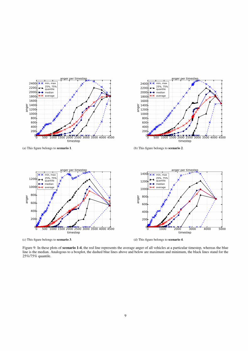
In contrary to that, the anger plots look quite different dependingon the fact, whether street priorities are enabled or not, as you cansee in the figures: Figure 9a and 9b look similar, Figure 9c and 9ddo so, too. The former two show, that the mood of the driver is fairlymoderate in the beginning of the simulation. The main differenceof Figure 9a and 9b towards Figure 9c and 9d lays in the generalmood, and especially, at the end of the simulation, where only about10 % of all drivers remain (see Figure 8). The general mood in thefigures with street priority enabled is up to twice as bad as it is inthe other ones, which is expressed by the maximum anger. The last10 % are a lot more angry in the first two scenarios. In this case, “alot” means, they have had to wait at least 1800 steps. Finishing theroute with an age of 4500 steps, the last remaining drivers have hadto wait around 40 % of their whole driving time.
We think, that the drivers are getting more angry in the middle ofthe simulation, since many drivers try to enter highways/motorways,where they have to wait for vehicles already driving on the high-way/motorway. It is in the middle of the simulation, because thedrivers have to get to the highway/motorway firstly.
In conclusion, street priorities seem to skew the waiting time ofvehicles, rather than distributing it uniformly, on the premise that thestreets are singlelaned. In addition to this, regarding our results ofthe anger plots, we would prefer only priority-to-the-right, becauseall drivers are less angry.
6.6 General traffic problemsWhile simulating different scenarios and cities, we noticed unre-solved overarching deadlocks. Our crossing logic handles deadlocksat one crossroad, but not spread over many crossroads. An exampleis shown in Figure 10.
In general, this deadlocks occurs in road networks including manysmall cycles, like in Stuttgart around roundabouts or in New Yorkwith its typical block structure. This is worse, if e.g. two roundabouts
8
0 500 1000 1500 2000 2500 3000 3500 4000 4500timestep
0
200
400
600
800
1000
1200
1400
1600
1800
2000
2200
2400
anger
anger per timestep
min, max25%, 75%quantilemedianaverage
(a) This figure belongs to scenario 1.
0 500 1000 1500 2000 2500 3000 3500 4000 4500timestep
0
200
400
600
800
1000
1200
1400
1600
1800
2000
2200
2400
anger
anger per timestep
min, max25%, 75%quantilemedianaverage
(b) This figure belongs to scenario 2.
0 500 1000 1500 2000 2500 3000 3500 4000 4500timestep
0
200
400
600
800
1000
1200
anger
anger per timestep
min, max25%, 75%quantilemedianaverage
(c) This figure belongs to scenario 3.
0 1000 2000 3000 4000 5000timestep
0
200
400
600
800
1000
1200
1400
anger
anger per timestep
min, max25%, 75%quantilemedianaverage
(d) This figure belongs to scenario 4.
Figure 9: In these plots of scenario 1-4, the red line represents the average anger of all vehicles at a particular timestep, whereas the blueline is the median. Analogous to a boxplot, the dashed blue lines above and below are maximum and minimum, the black lines stand for the25%/75% quantile.
9

Figure 10: This deadlock is located in Tokyo, but it is representivefor small cycles in cities’ road networks. Especially with muchtraffic, this kind of traffic jam occurs frequently.
are next to each other, connected by a bidirectional street. In thecase, this construct is heavily used, it can cause massive traffic jams.
7 CONCLUSIONS
We explained, which demands are put forth by our traffic model andhow we could fulfill these by using OpenStreetMap data. Besidesdescribing the visualization aspect in detail, e.g. the layer organisa-tion or line joins, we mentioned the projection of the map data andhow we extracted important information from the OSM XML files.
Our traffic model is based on the popular Nagel-Schreckenbergmodel, which is a microscopic approach using a cellular automaton.Our traffic rules contain priority-to-the-right (or left) and streetpriorities. We added an anger to the vehicles, representing a counterof how much time a vehicle has to wait during its route. This angercould show, that different traffic rules do not influence the averagewaiting time, but the distribution, how many vehicles have to wait acertain time. Furthermore, we detected problems of heavily usedstreets, which form a cycle. The smaller the cycles, the higher is thechance of detecting overarching deadlocks.
Future work is the implementation of multilaned streets andtraffic lights, to obtain even more realistic simulation results. Fornow, our bottleneck is the route calculation in the preprocessing.We are planning the use of contraction hierarchies. These needtheir own preprocessing, which depends on the used map, but theroute calculation can be done much faster. This would allow us toimplement dynamic routing, whereas our routing is still static.
An additional future feature is the use of a graphical user interfacefor our simulation, which let the user control simulation parametersand measured data. We also plan a serialization of preprocesseddata like map data to seperate the preprocessing from the simulationitself.
REFERENCES
[1] E. W. Dijkstra. A Note on Two Problems in Connexion with Graphs,pages 269 – 271. 1959.
[2] P. E. Hart, N. J. Nilsson, and B. Raphael. A Formal Basis for the HeuristicDetermination of Minimum Cost Paths, pages 100 – 107. 1968.
[3] INRIX. Jahrliche INRIX Traffic Scorecard – Wichtigste Ergebnisse.http://inrix.com/scorecard/key-findings-de/. Ac-cessed: 2016-04-12.
[4] K. Nagel and M. Schreckenberg. A cellular automaton model for freewaytraffic, pages 2221 – 2229. 1992.
[5] OpenStreetMap Wiki. https://wiki.openstreetmap.org.Accessed: 2016-03-27.
[6] J. P. Snyder. Map Projections Used by the U.S. Geological Survey.Technical Report 1532, U.S. Geological Survey, 1982.
10