Microscopic theory of memory functions

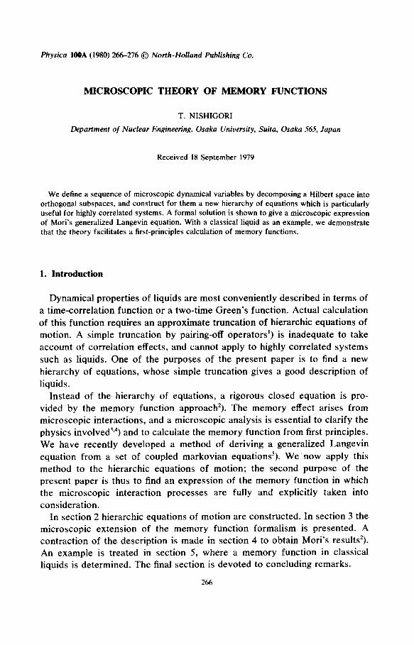
Physica 1OOA (1980) 266-276 @ North-Holland Publishing Co.

MICROSCOPIC THEORY OF MEMORY FUNCTIONS

T. NISHIGORI

Department of Nuclear Engineering, Osaka University, Suita, Osaka 565, Japan

Received 18 September 1979

We define a sequence of microscopic dynamical variables by decomposing a Hilbert space into orthogonal subspaces, and construct for them a new hierarchy of equations which is particularly useful for highly correlated systems. A formal solution is shown to give a microscopic expression of Mori’s generalized Langevin equation. With a classical liquid as an example, we demonstrate that the theory facilitates a first-principles calculation of memory functions.

1. Introduction

Dynamical properties of liquids are most conveniently described in terms of a time-correlation function or a two-time Green’s function. Actual calculation of this function requires an approximate truncation of hierarchic equations of motion. A simple truncation by pairing-off operators’) is inadequate to take account of correlation effects, and cannot apply to highly correlated systems such as liquids. One of the purposes of the present paper is to find a new hierarchy of equations, whose simple truncation gives a good description of liquids.

Instead of the hierarchy of equations, a rigorous closed equation is pro- vided by the memory function approach*). The memory effect arises from microscopic interactions, and a microscopic analysis is essential to clarify the physics involved3v4) and to calculate the memory function from first principles. We have recently developed a method of deriving a generalized Langevin equation from a set of coupled markovian equations’). We now apply this method to the hierarchic equations of motion; the second purpose of the present paper is thus to find an expression of the memory function in which the microscopic interaction processes are fully and explicitly taken into consideration.

In section 2 hierarchic equations of motion are constructed. In section 3 the microscopic extension of the memory function formalism is presented. A contraction of the description is made in section 4 to obtain Mori’s results2). An example is treated in section 5, where a memory function in classical liquids is determined. The final section is devoted to concluding remarks.

266

MICROSCOPIC THEORY OF MEMORY FUNCTIONS 267

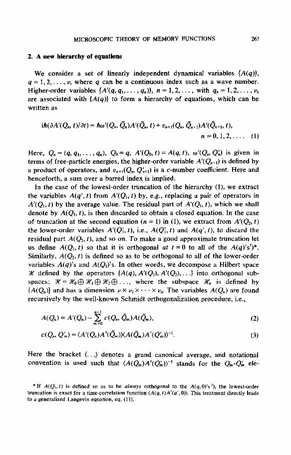
2. A new hierarchy of equations

We consider a set of linearly independent dynamical variables {A(q)},

4=1,2,..., V, where 4 can be a continuous index such as a wave number. Higher-order variables {A’(q, 41, . . . , q.)}, n = 1,2,. . . , with 4. = 1,2,. . . , v,

are associated with {A(q)} to form a hierarchy of equations, which can be written as

iMaA’(Q,, O/W = h~‘(Ch, &A’(on, 0 + G+I(Q., ~n+~M’(~n+~, 0, n=0,1,2 ).... (1)

Here, Qn = (4, a,. . . , 4,,), QO = 4, A’(% t) = A(4,0, w’(Q., Q3 is given in terms of free-particle energies, the higher-order variable A’(Q+J is defined by a product of operators, and u,+r(Q, QL+r) is a c-number coefficient. Here and henceforth, a sum over a barred index is implied.

In the case of the lowest-order truncation of the hierarchy (l), we extract the variables A(q’, t) from A’(Q,, t) by, e.g., replacing a pair of operators in A’(Q,, t) by the average value. The residual part of A’(Q,, t), which we shall denote by A(QI, t), is then discarded to obtain a closed equation. In the case of truncation at the second equation (n = 1) in (l), we extract from A’(@, t)

the lower-order variables A’(Q;, t), i.e., A(Q;, t) and A(q’, t), to discard the residual part A(Q,, t), and so on. To make a good approximate truncation let us define A(@, t) so that it is orthogonal at t = 0 to all of the A(4)‘?)*. Similarly, A(& t) is defined so as to be orthogonal to all of the lower-order variables A(q)‘s and A(QJs. In other words, we decompose a Hilbert space X defined by the operators {A(4), A’(Q), A’(@. . . .} into orthogonal subspaces; X=%)@X,$XZ$..., where the subspace X,, is defined by {A(Q)} and has a dimension v x vl x . . . x vn. The variables A(Qn) are found recursively by the well-known Schmidt orthogonalization procedure, i.e.,

(2) m=O

c(Qn, QLJ = (A’(Q,)A+(~~))(A(~~)A+(~~))-‘. (3)

Here the bracket (. . .) denotes a grand canonical average, and notational convention is used such that (A(Qm)A stands for the Q&L, ele-

* If A(Q,, t) is defined so as to be always orthogonal to the A(q,O)‘s *). the lowest-order truncation is exact for a time-correlation function (A(q, t)A’(q’, 0)). This treatment directly leads to a generalized Langevin equation, eq. (11).

268 T. NISHIGORI

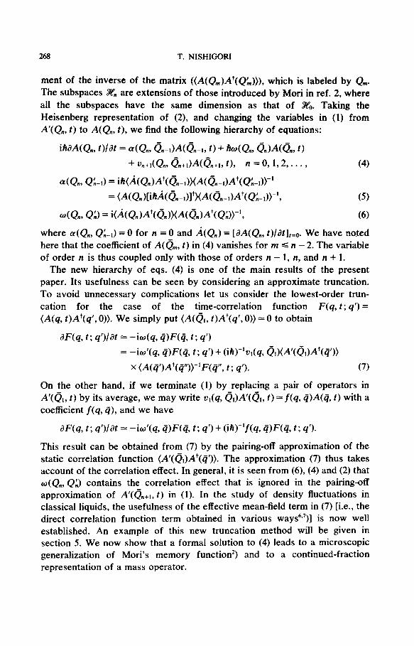
ment of the inverse of the matrix ((A(Q,)A which is labeled by Q,,,. The subspaces 3% are extensions of those introduced by Mori in ref. 2, where all the subspaces have the same dimension as that of X0. Taking the Heisenberg representation of (2), and changing the variables in (1) from A’(Qn, t) to A(Q,, t), we find the following hierarchy of equations:

ihMQ,, O/at = 4Q,, &M(~,-I, 0+~4Qn,~nM(~n,~) + ~+dQn, ~n+,M~n+,, t), n =O, I,&..., (4)

4Qn, QL) = i~(~(Q,)A'(~~-~)XA(~~-~)A'(Q:-I))-' = (A(Q,)[ihA(~"-,)I')(A(~"-,)A+(Q~-,))-', (5)

4Qn9 QA) = i(A(Q.)At(~",)XA(~,)At(Q3)-', (6)

where a(Q., QA_,) = 0 for n = 0 and A(Q”) = [aA(Q., t)/dt],=,. We have noted here that the coefficient of A(& t) in (4) vanishes for m s n - 2. The variable of order n is thus coupled only with those of orders n - 1, n, and n + 1.

The new hierarchy of eqs. (4) is one of the main results of the present paper. Its usefulness can be seen by considering an approximate truncation. To avoid unnecessary complications let us consider the lowest-order truncation for the case of the time-correlation function F(4, t; 4’) = (A(4, t)A’(q’, 0)). We simply put (A(Q,, t)A+(q’, 0)) = 0 to obtain

@(s, r; 4’)lat = -iw(4, iiF(4, t; 4’)

= -iw’(4,4)F(4, t; 4’) + (ifi)-‘vl(4, Q1)(A’(Q9At(4’))

x (A(q’-‘F(q”, t; 4’). (7)

On the other hand, if we terminate (1) by replacing a pair of operators in A’(Q,, t) by its average, we may write vr(4, @A’<QI, t) -f(4, tj)A(q, t) with a coefficient f(4,4), and we have

~334, t ; 4’)lat = -io’(4,4)F(4, r ; 4’) + (ifi)-‘f(4,4F(4, r ; 4’).

This result can be obtained from (7) by the pairing-off approximation of the static correlation function (A’(QI)At(ij’)). The approximation (7) thus takes account of the correlation effect. In general, it is seen from (6), (4) and (2) that w(Qn, QA) contains the correlation effect that is ignored in the pairing-off approximation of A’( on+, , t) in (1). In the study of density fluctuations in classical liquids, the usefulness of the effective mean-field term in (7) [Le., the direct correlation function term obtained in various ways6*‘)1 is now well established. An example of this new truncation method will be given in section 5. We now show that a formal solution to (4) leads to a microscopic generalization of Mori’s memory function*) and to a continued-fraction representation of a mass operator.


3. Microscopic memory function

3.1. The generalized Langevin equation

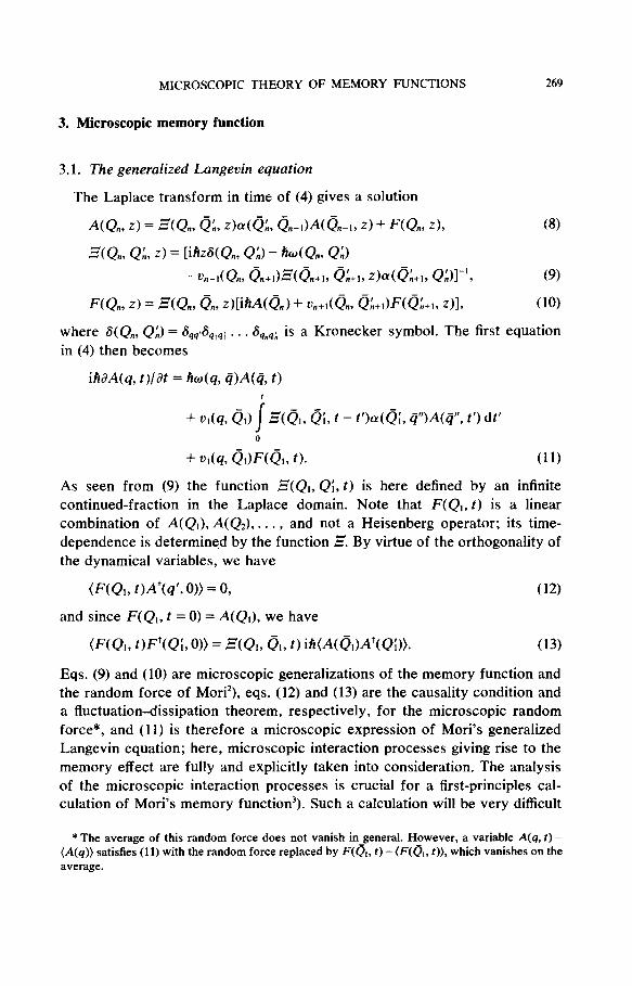
The Laplace transform in time of (4) gives a solution

A(Q”, z) = E(Qn, 0;. z)c&, Q”-,)&&I, z) + F(Q.9 z), (8)

B(Q”, Q;, 2) = [ihzWQn, Q3 - WQn, Q3

- u.+dQn, ~n+,>E@n+,, ~L+I, zMQA+I, QX’, (9)

F(Qn, z) = ECQ,, o,,, z)WUQ,) + G+I(& ~A+M’(QA+I, z)l, (10)

where S(Qn, Q3 = &P%,,; . . . hn4; is a Kronecker symbol. The first equation

in (4) then becomes

ihaA(q, t)/at = hw(q, #A(Q, t)

+ Vl(4, a,> I s(& 0;. t - t’)&, @‘)A(@‘, t’) dt’ 0

+ d4, QMm, t). (11)

As seen from (9) the function B(Q,, Q;, t) is here defined by an infinite continued-fraction in the Laplace domain. Note that F(Qr, t) is a linear combination of A(Q,), A(Q2), . . . , and not a Heisenberg operator; its time- dependence is determined by the function g. By virtue of the orthogonality of the dynamical variables, we have

and

#IQ,, tM+(q’, ON = 0,

since F(Q,, t = 0) = A(Q,), we have

(12)

V’(QI, tFt(QL 0)) = %QI, QI, t) WA(QJAt(Q9). (13)

Eqs. (9) and (10) are microscopic generalizations of the memory function and the random force of Mori’), eqs. (12) and (13) are the causality condition and a fluctuation-dissipation theorem, respectively, for the microscopic random force*, and (11) is therefore a microscopic expression of Mori’s generalized Langevin equation; here, microscopic interaction processes giving rise to the memory effect are fully and explicitly taken into consideration. The analysis of the microscopic interaction processes is crucial for a first-principles calculation of Mori’s memory functior?). Such a calculation will be very difficult

* The average of this random force does not vanish in-general. H_owever, a variable A(q, t) - (A(q)) satisfies (11) with the random force replaced by F(Q,, t) - (F(Q,, t)), which vanishes on the

average.

270 T. NISHIGORI

if we use Mori’s expression, which is a contracted description as will be seen in section 4.

3.2. A mass operator

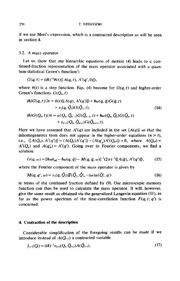
Let us show that our hierarchic equations of motion (4) leads to a continued-fraction representation of the mass operator associated with a quantum-statistical Green’s function’)

G(q, t) = (ih)-‘(Vt)([A(q, t), A+(q’, ON),

where O(t) is a step function. Eqs. (4) become for G(q, t) and higher-order Green’s functions G(Q., t)

ihJG(q, t)/Jt = W([A(q), At(q + Wq, 4M4, t)

+ da QWt& t),

ifiaG(Q,, t)/Jt = a(% &)G(&, 0 + WC&, 6X(& r)

+ u.+,(Qn, en+,)G(on+,, t).

(14)

Here we have assumed that At(q) are included in the set {A(q)} so that the inhomogeneous term does not appear in the higher-order equations (n 3 l),

i.e., ([A(Q), At(q = (A(Q,Mt(4N - (A(q’,Mt(Qn*N = 0, where NC&) = At(Q) and A(q’,) = A+(q’). Going over to Fourier components, we find a solution

G(q, 0) = [fiti& - fiw(q, (5) - M(q, 4, w)l-‘(277-‘(M4), At(q’ (15)

where the Fourier component of the mass operator is given by

M(q, 4’, W) = vl(q, QI)Z(QI, Qr, -iw)cw(QI, 4’) (16)

in terms of the continued fraction defined by (9). Our microscopic memory function can thus be used to calculate the mass operator. It will, however, give the same result as obtained via the generalized Langevin equation (I I), as far as the power spectrum of the time-correlation function F(q, t; q’) is concerned.

4. Contraction of the description

Considerable simplification of the foregoing results can be made if we introduce instead of A(Q+,) a contracted variable

f,+i(Q) = (ih)%+i(Q,, (?,+,)A(o,+i), (17)

MICROSCOPIC THEORY

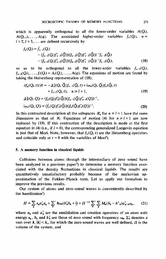
which is apparently orthogonal to

A(QI-I), . . . , A(q). The associated 1+2,1+3,... are defined recursively

fn(Q,) = in-dQ,)

OF MEMORY FUNCTIONS 271

all the lower-order variables A(Q,), higher-order variables f,, (QI), n =

by

- (f,-,tQ~>ft-2(~~)>(fn-,<Q;)f~-2(~,I))-’fn-2(~,1)

- ~“-,(Q,)f~-,(Q;))(f.-,(~~)~~-,(~,l))-’fn-,(~,l), (18)

so as to be orthogonal to all the lower-order variables f,,_r(Q,),

fn-I, . . . 3 f,(Q,) = MQ,), . . . , A(q). The equations of motion are found by taking the Heisenberg representation of (18);

af.(Q~, r)/Jr = -AXQ,, Ql)f”-l(Ql, 0 + io,(QI, Ql)fAQj, t)

+ fn+~(Q/, t), n 3 I+ 1, (19)

&(Q,t Q;) = (fn(Q,lftn(~,r))Cfn-,(~,)~~-,(Q;))-’,

h(Q,, Qi) = (fn(Q,>f~(~,>>(fn<Q>f~(Q~))-‘. (20)

In this contracted description all the subspaces SY,, for n 2 I+ 1 have the same dimension as that of X,. Equations of motion (4) for n 2 I+ 1 are now replaced by (19). If this contraction of the description is made at the first equation in (4) (i.e., if 1 = O), the corresponding generalized Langevin equation is just that of Mori. Note, however, that fn(QI, t) are the Heisenberg operators and coincide only at t = 0 with the variables of Mori2).

5. A memory function in classical liquids

Collisions between atoms through the intermediary of zero sound have been analyzed in a previous paper3) to determine a memory function associated with the density fluctuations in classical liquids. The results are quantitatively unsatisfactory probably because of the markovian approximation of the Fokker-Planck term. Let us apply our formalism to improve the previous results.

Our system of atoms and zero-sound waves is conveniently described by the hamiltonian3)

H = z l &, + F’ hok(b:bt +:> + W2 F’ 2 M,(bL - bt&:+@, , (21) q Q

where a, and u: are the annihilation and creation operators of an atom with energy 4, bk and b: are those of zero sound with frequency wL, Xi denotes a sum over k, Ikj < k,, for which the zero-sound waves are well defined, R is the volume of the system, and

272 T. NISHIGORI

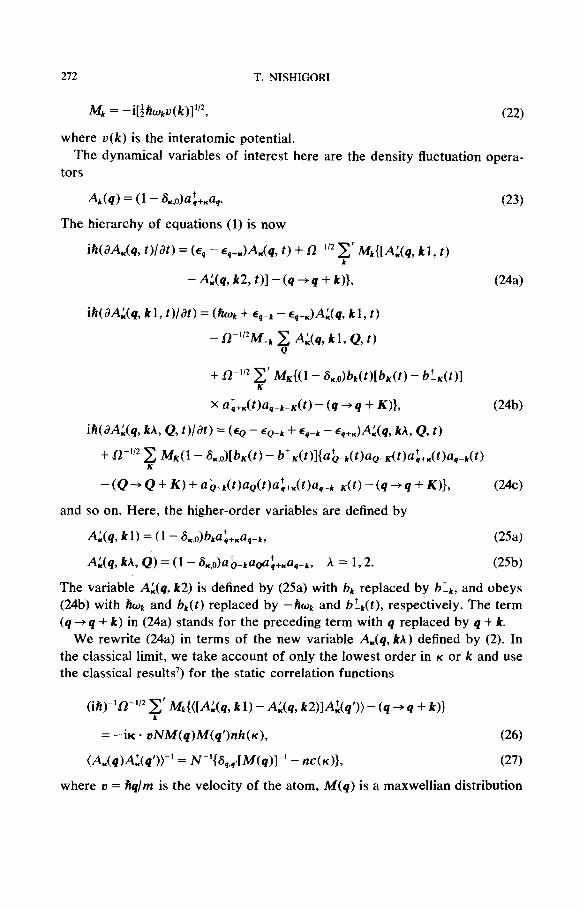
Mk = -i[#okv(k)]1’2, (22)

where u(k) is the interatomic potential. The dynamical variables of interest here are the density fluctuation opera-

tors

A,(q) = (1 - &,~)q:+,q~

The hierarchy of equations (1) is now

ik(aA,(q, O/at) = (e4 - Eq+K)AI(q, r) + O-“’ 2 MOAXq, kl, t) k

(23)

- &(a k2, t)l - (4 -+ 4 + k)I, CW

ih(JAL(q, kl, t)/iV) = (hk + l g-k - l ,+,)AL(q, kl, t)

- fi-“*hf_k 5 A:(q, kl, Q, t)

+ 0-l’” x’ k&&l - &.O)bk(t)[bK(t) - b:,(t)]

x a;+&;a,-k-K(f ) - (4 --, 4 + K)}, Wb)

iWW(q, k& Q, t)/at) = (6 - EQ-k + 4-k - l ,+,)Mq, kh, Q, f)

+ n-“* x MK(1 - &,O)[bK(t) - b’K(t)l{d-k(t)aQ-K(t)a:,,oa,_L(t) K

- (Q --, Q + K) + &k(t)aQ(t)a:+&)&,-k-K(t) - (4 + 4 + K)),

and so on. Here, the higher-order variables are defined by

A:(q, kl) = (1 - &O)bk~:+&-k,

A:(q, k& Q) = (I- &,O)d.-kQ@:+,&k, A = 1,2.

(24~)

(254

(25b)

The variable A:(q, k2) is defined by (25a) with bk replaced by btk, and obeys (24b) with hwk and b,(t) replaced by -fiwk and b:,(t), respectively. The term (q + q + k) in (24a) stands for the preceding term with q replaced by q + k.

We rewrite (24a) in terms of the new variable A,(q, kh) defined by (2). In the classical limit, we take account of only the lowest order in K or k and use the classical results’) for the static correlation functions

(ifi-‘R-“* F’ MkMAXq, k 1) - AXq, WlA,i(q’)) - (q + q + k))

= -iK * UNhf(q)M(q’)dl(K), (26)

(&(q)A:(q’))- = I’-‘@q,,~[~(q)l-’ - dK)h (27)

where u = hq/m is the velocity of the atom, M(q) is a maxwellian distribution

T. NISHIGORI 273

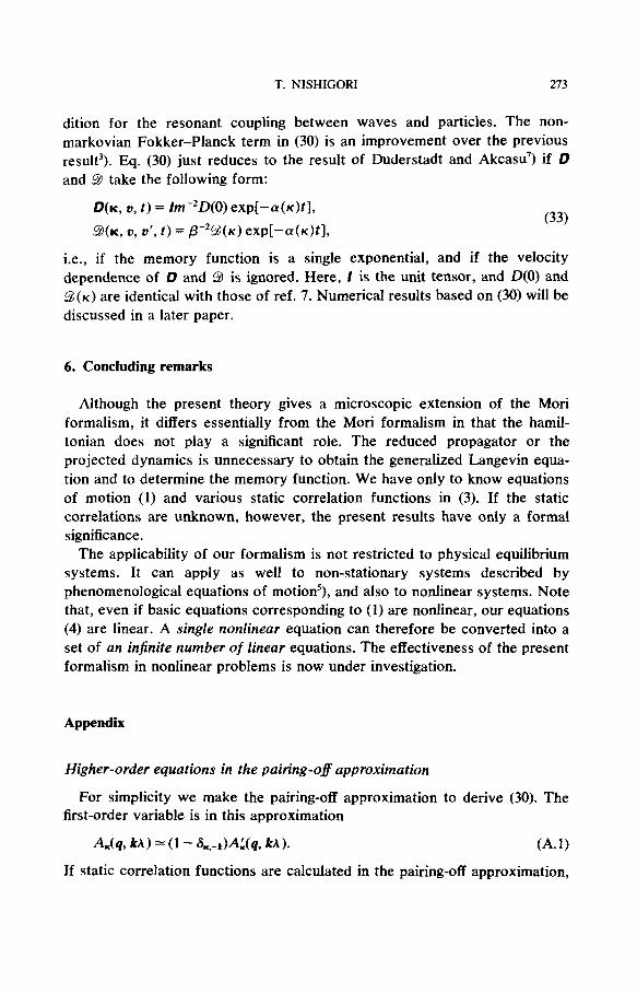
dition for the resonant coupling between waves and particles. The non- markovian Fokker-Planck term in (30) is an improvement over the previous result’). Eq. (30) just reduces to the result of Duderstadt and Akcasu’) if D and 9 take the following form:

D(K, u, t) = Im-*D(O) exp[-cY(K)tl,

9(K,U,D', f)= ,6-*~(K)exp[-a(K)f], (33)

i.e., if the memory function is a single exponential, and if the velocity dependence of D and 9 is ignored. Here, I is the unit tensor, and D(0) and 9(~) are identical with those of ref. 7. Numerical results based on (30) will be discussed in a later paper.

6. Concluding remarks

Although the present theory gives a microscopic extension of the Mori formalism, it differs essentially from the Mori formalism in that the hamiltonian does not play a significant role. The reduced propagator or the projected dynamics is unnecessary to obtain the generalized Langevin equation and to determine the memory function. We have only to know equations of motion (1) and various static correlation functions in (3). If the static correlations are unknown, however, the present results have only a formal significance.

The applicability of our formalism is not restricted to physical equilibrium systems. It can apply as well to non-stationary systems described by phenomenological equations of motion’), and also to nonlinear systems. Note that, even if basic equations corresponding to (1) are nonlinear, our equations (4) are linear. A single nonlinear equation can therefore be converted into a set of an infinite number of linear equations. The effectiveness of the present formalism in nonlinear problems is now under investigation.

Appendix

Higher-order equations in the pairing-of approximation

For simplicity we make the pairing-off approximation to derive (30). The first-order variable is in this approximation

A&, U) = (1 - &,-k)A:(q, kA ). (A.1)

If static correlation functions are calculated in the pairing-off approximation,

274 MICROSCOPIC THEORY OF MEMORY FUNCTIONS

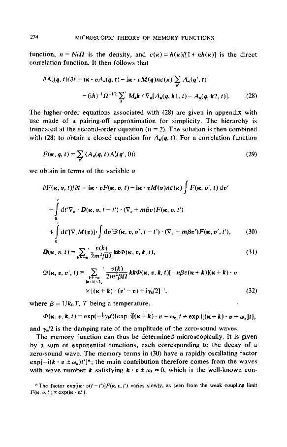
function, n = N/L! is the density, and C(K) = h(~)/[l + n/z(~)] is the direct correlation function. It then follows that

dA,(q, t)/dt = iK - uA.(q, t) - ire. df(q)nC(K) c A,(q’, t) B’

- (ih)-‘R-“2 T’ M,k ;V,[A,(q, kl, t) - A,(q, k2, t)]. (28)

The higher-order equations associated with (28) are given in appendix with use made of a pairing-off approximation for simplicity. The hierarchy is truncated at the second-order equation (n = 2). The solution is then combined with (28) to obtain a closed equation for A,(q, t). For a correlation function

F(K, 4, t) = 3 (A,(q, tMic(q’, 0))

we obtain in terms of the variable u

(2%

d&K, 11, t)/dt = iK * UF(K, 0, t) - iK * uitf(u)nc(~) F(K, u’, t) du’

I

+ I

dt’V, - &K, U, t - t’) * (v, + @U)F(K, U, t’)

0

+ 1 dt’[V,M(u)] j- du’9( K, 0, U’, t - t’) ’ (v,, + @U’)F(K, U’, t’), (30) 0

D(K, u, t) = ,& & kk@(K, u, k, t), (31)

g(K 0, n’, r) = & ’ & kk@(K, u, k, t)[- @I(# + k)](K + k) * u

Jr+kl<k,

x [(K + k) * (U’ - U) + iyk/2]-‘, (32)

where p = l/kBT, T being a temperature,

@(K, 0, k, t) = eXp(-iykt){eXp i[(K + k) * u - Wk]t + exp i[(K + k) * u + w&},

and ‘j&/2 is the damping rate of the amplitude of the zero-sound waves. The memory function can thus be determined microscopically. It is given

by a sum of exponential functions, each corresponding to the decay of a zero-sound wave. The memory terms in (30) have a rapidly oscillating factor exp[-i(k - u 2 b&)t’]*; the main contribution therefore comes from the waves with wave number k satisfying k * u f Wk = 0, which is the well-known con-

* The factor exp[iK * o(t - ~‘)]F(K, o, t’) varies slowly, as seen from the weak coupling limit

F(K, u, t’) a exp(iw . ut’).


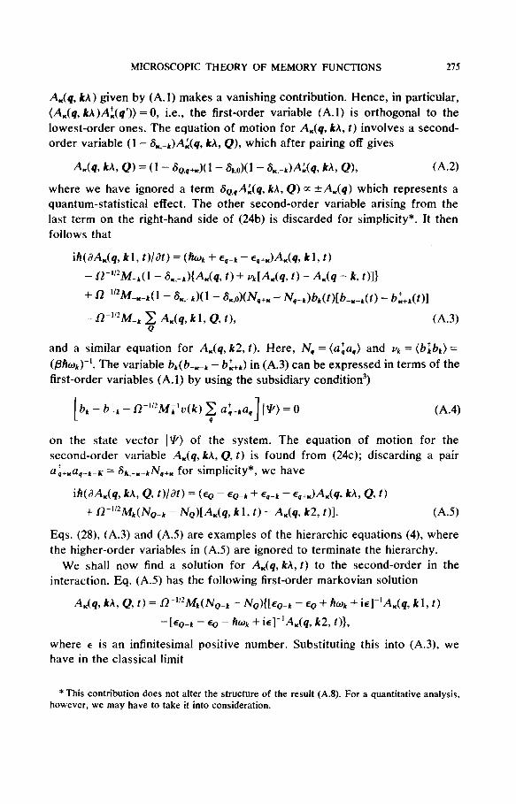
A,(q, rkh) given by (A.l) makes a vanishing contribution. Hence, in particular, (A,(q, kA)Al(q’)) =O, i.e., the first-order variable (A.l) is orthogonal to the lowest-order ones. The equation of motion for A.(q, kA, t) involves a second- order variable (I - S,+)A:(q, M, Q), which after pairing off gives

A.z(q, f& Q) = (I- So.,+,)(l - &ON - &&A:(q, kA, Q), (A.2)

where we have ignored a term 6,,A:(q, kh, Q) 0: *A,(q) which represents a quantum-statistical effect. The other second-order variable arising from the last term on the right-hand side of (24b) is discarded for simplicity*. It then

follows that

ih(aA,(q, k 1, t)/dt) = (hw + E~-L - Eliu)Ar(q, k 1, t)

- O-“zM-dl - S,.-d{A,(q, t) + dA,(q, f) - A,(q - k, t)lI

+ ‘-“zM-E-.dl - &-k)(l - &,d(&+, - Nq-k)bk(t)[b_,_k(t) - b:+,(t)]

- fl-“*M-k 3 Adq, k 1, Q, t). (A.3)

and a similar equation for A.(q, k2, t). Here, Nq = (~:a,) and vk = (b:b,) =

@%J$‘. The variable bk(b_,_k - bt+k) in (A.3) can be expressed in terms of the first-order variables (A.l) by using the subsidiary condition3)

[hk - bt, - ii-“*hf;‘u(k) c C&U,] I?@) = 0 (A.4) P

on the state vector I!@ of the system. The equation of motion for the second-order variable A,(q, kh, Q, t) is found from (24~); discarding a pair

+ aq+K+_K = 8K,_r_k~q+g for simplicity*, we have

iWaA,(q, kh, Q, t)/at) = (6 - EQ-k + 4-k - l ,+.)A(q, kA, Q, r)

+ fi-“*Mk(NQ-k - NQ)[&(q, k 1, t) - Adq, k2, t)l. (A.3

Eqs. (28), (A.3) and (AS) are examples of the hierarchic equations (4), where the higher-order variables in (AS) are ignored to terminate the hierarchy.

We shall now find a solution for A,(q, kh, t) to the second-order in the interaction. Eq. (AS) has the following first-order markovian solution

A.(q, kh, Q, t) = ii-“*b&(&, - NQ){[EQ-k - 6 + hWk + ie]-‘A,(q, kl, t)

-[6-k - EQ - h6& + ie]-‘A,(q, k2, t)},

where 4 is an infinitesimal positive number. Substituting this into (A.3), we have in the classical limit

* This contribution does not alter the structure of the result (A.8). For a quantitative analysis, however, we may have to take it into consideration.

T. NISHIGORI

JA,(q, kl, t)/at = -i[wk -(K+ k). u +&I~ -iyk)]A,(q, kl, t)

+ ib + ix)&(q, G t)

- (ih)-‘R-“2M_L( 1 - S,,_,)( 1 + vkk . V,)A,(q, t)

+ (ih)-‘(K + k) . V,ibf(q)fW(K+ k) c A,(q’, kl, t), (~4.6) Q’

where (K + kj < k,, and pk and 3/k are defined by

(A.7)

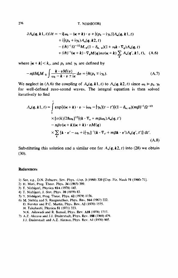
We neglect in (A.6) the COUpiing Of A,(q, k 1, t) t0 A,(q, k2, t) SinCe wk S pk, yk

for well-defined zero-sound waves. The integral equation is then solved iteratively to find

f . A,(q, kl, t) = J exp{i(K+ k) ’ 0 -iOk -$j$.](t - t’)}(l - &_k)(mp)-'~-"2

0

x [dk)/2b]"2{(k *v, + @w)A.(q, t')

- n@(lc + k)(K + k) - uM(q)

X c [k * u’ - ‘I& + i&-‘(k * v,, + tnpk * u’)Ai,(q’, t’)} dt’. q’

(A.8)

Substituting this solution and a similar one for A,(q, k2, t) into (28) we obtain

(30).

References

1) See, e.g., D.N. Zubarev, Sov. Phys. -Usp. 3 (1960) 320 [Usp. Fiz. Nauk 71 (1960) 71). 2) H. Mori, Prog. Theor. Phys. 34 (1965) 399. 3) T. Nishigori, Physica 92A (1978) 145. 4) T. Nishigori, J. Stat. Phys. 20 (1979) 83. 5) T. Nishigori, Prog. Theor. Phys. 62 (1979) 1156. 6) M. Nelkin and S. Ranganathan, Phys. Rev. 164 (1967) 222.

D. Forster and P.C. Martin, Phys. Rev. A2 (1!?70) 1575. H. Takahashi, Physica 51 (1971) 333. N.K. Ailawadi and R. Bansal, Phys. Rev. A18 (1978) 1717.

7) A.Z. Akcasu and J.J. Duderstadt, Phys. Rev. 188 (1%9) 479. J.J. Duderstadt and A.Z. Akcasu, Phys. Rev. Al (1970) 905.

Documents

Microscopic theory of memory functions