MICROSCOPIC THEORY OF

SUPERCONDUCTIVITY

by

Helmut Eschrig

(2001, updated 08/2008)

These lecture notes are dedicatedto Dierk Rainer

on the occassion of his 60th birthday in 2001.He pioneered the systematic treatment

of the low-energy scale in theelectronic theory of condensed matter.

2

Contents

1 The Solid as a Quantum Many-Body System 4

1.1 The Coulomb Hamiltonian of the Solid . . . . . . . . . . . . . . . . . . . . . . . . . . 4

1.2 Reduced Density Matrices and Densities . . . . . . . . . . . . . . . . . . . . . . . . . 7

1.3 Correlation Functions . . . . . . . . . . . . . . . . . . . . . . . . . . . . . . . . . . . 9

2 Green’s Functions 13

2.1 Spectral Representation . . . . . . . . . . . . . . . . . . . . . . . . . . . . . . . . . . 14

2.2 Equation of Motion . . . . . . . . . . . . . . . . . . . . . . . . . . . . . . . . . . . . . 17

2.3 Complex Time . . . . . . . . . . . . . . . . . . . . . . . . . . . . . . . . . . . . . . . 19

2.4 The Interaction Picture . . . . . . . . . . . . . . . . . . . . . . . . . . . . . . . . . . 21

2.5 Wick’s Theorem . . . . . . . . . . . . . . . . . . . . . . . . . . . . . . . . . . . . . . 24

2.6 Feynman Diagrams . . . . . . . . . . . . . . . . . . . . . . . . . . . . . . . . . . . . . 26

2.7 The Self-Energy . . . . . . . . . . . . . . . . . . . . . . . . . . . . . . . . . . . . . . . 28

2.8 Thermodynamic Quantities . . . . . . . . . . . . . . . . . . . . . . . . . . . . . . . . 30

3 Green’s Functions in the Superconducting State 31

3.1 The Bogoliubov-Valatin Transformation . . . . . . . . . . . . . . . . . . . . . . . . . 32

3.2 The Nambu Structure . . . . . . . . . . . . . . . . . . . . . . . . . . . . . . . . . . . 34

3.3 Green’s Functions and Vertices for the Electron-Nucleon System . . . . . . . . . . . 35

4 Split-off of High-Energy Parts 39

4.1 Classification of Primary Diagrams . . . . . . . . . . . . . . . . . . . . . . . . . . . . 39

4.2 Migdal’s Theorem . . . . . . . . . . . . . . . . . . . . . . . . . . . . . . . . . . . . . 42

4.3 Leading Order Self-Energies . . . . . . . . . . . . . . . . . . . . . . . . . . . . . . . . 44

5 The Low Energy Equations 46

5.1 The Quasi-Particle Renormalization . . . . . . . . . . . . . . . . . . . . . . . . . . . 47

5.2 The Electron-Phonon Self-Energy . . . . . . . . . . . . . . . . . . . . . . . . . . . . . 48

5.3 The Electron-Electron Self-Energy . . . . . . . . . . . . . . . . . . . . . . . . . . . . 49

5.4 Bloch Function Representation on the Fermi Surface . . . . . . . . . . . . . . . . . . 49

6 Strong Coupling Theory of the Transition Temperature 53

6.1 Linearization of Eliashberg’s Equations . . . . . . . . . . . . . . . . . . . . . . . . . . 53

6.2 The Tc Formula . . . . . . . . . . . . . . . . . . . . . . . . . . . . . . . . . . . . . . . 55

6.3 The Dirty Limit . . . . . . . . . . . . . . . . . . . . . . . . . . . . . . . . . . . . . . 56

6.4 The Cut-Off Frequency . . . . . . . . . . . . . . . . . . . . . . . . . . . . . . . . . . 58

7 Physical Properties of the Superconducting State 59

7.1 Eliashberg’s Non-Linear Equations . . . . . . . . . . . . . . . . . . . . . . . . . . . . 59

7.2 The Quasiparticle Density of States . . . . . . . . . . . . . . . . . . . . . . . . . . . 62

7.3 The Thermodynamic Critical Field . . . . . . . . . . . . . . . . . . . . . . . . . . . . 63

3

Chapter 1

The Solid as a Quantum

Many-Body System

Physics as a unifying science tends to trace back all empirical phenomena to a small numberof fundamental principles. The microscopic theory of superconductivity is an excellent exam-ple of a steady seventy years progress towards this goal which is still further going on. Theselectures attempt at a concise description of what has been achieved so far in this directionfor the understanding of the electron-phonon mechanism of superconductivity. We take asa staring point the non-relativistic Hamiltonian with Coulomb interactions of electrons andnuclei, although, strictly speaking, this is already a model. However, relativistic kinematicsleading to mass corrections, Darwin’s contact interaction, spin-orbit coupling and spin-spindipolar interaction (including hyperfine interaction with the nuclear spin) may later on beadded as correction terms, and replacement of the Coulomb interaction by the relativisticphoton exchange or consideration of internal nuclear degrees of freedom would practicallynot change any of the considered results.

The first fully satisfactory treatment of the theory starting from this Hamiltonian wasgiven by Dierk Rainer1 in 1986, just in the year of discovery of high temperature supercon-ductivity of the cuprates, which latter has put a completely new and up to now essentiallyunsolved problem for such a type of theory. The early microscopic theory of superconduc-tivity2 was led back to the use of the Frohlich Hamiltonian of electrons and phonons, amodel Hamiltonian which cannot be derived from many-body theory and which has to beused with caution by following certain model recipes. Later on, the elctron-ion system wasproperly treated field theoretically,3 but still the separation of the low energy scale was notmade completely explicit.

1.1 The Coulomb Hamiltonian of the Solid

As mentioned above, we take as the starting point the Hamiltonian

H = t+ Vee + Ven + Vnn + T , (1.1)

1D. Rainer, in: D. F. Brewer (ed.), Progress in Low Temperature Physics, vol. X, p. 371, Elsevier,Amsterdam 1986.

2G. M. Eliashberg, Sov. Phys.-JETP 11, 696 (1960); 12, 1000 (1961).3D. Scalapino, in: R. D. Parks (ed.), Superconductivity, vol. 1, p. 449, Dekker, New York 1969.

4

where

t = −N∑

i=1

1

2

∂2

∂r2i

(1.2)

is the operator of the kinetic energy of the N electrons,

Vee =1

2

N∑

i6=j

1

|ri − rj |(1.3)

is the operator of the electron-electron interaction,

Ven = −N∑

i=1

M∑

m=1

Zm

|ri − Rm| (1.4)

is the operator of the interaction of the electrons with the M nuclei of charges Zm,∑

m Zm =N ,

Vnn =1

2

M∑

m 6=n

ZmZn

|Rm − Rn|(1.5)

is the operator of the nucleus-nucleus interaction, and

T = −M∑

m=1

1

2Mm

∂2

∂R2m

(1.6)

is the operator of the kinetic energy of the nuclei.We used natural atomic units

~ = |e| = me = 1a.u., Mm ≡ mm

me≈ 103 · · · 105,

〈T 〉〈t〉 ≈ 〈M〉−1/2 ≡ α, α ≈ 10−2. (1.7)

The last estimate is the result of the well known Born-Oppenheimer perturbation theory.The presence of the small parameter α will play a key role in all what follows. It allows tosplit the Hamiltonian according to H = H0 + H1 into a zero-order part H0 and the rest. Tothis end, reference positions R0

m of nuclei with a lattice spacing a are introduced in such away that the nuclear displacements um remain small all the time:

Rm = R0m + um,

( 〈um〉a

)2

∼ α. (1.8)

In addition we change the Hamiltonian into a grand canonical one by adding a chemicalpotential term for the electrons. (Since the nuclear wavefunctions do practically not overlap,their statistics need not be taken into consideration.4) Then we have

H0 = t+ Vee + Ven(R0m) + Vnn(R0

m) − µN, (1.9)

where Vnn(R0m) is now just a constant number, N is the operator of the number of electrons,

and µ is the chemical potential of the electrons. The number of electrons need not be fixedany more, instead

∑

m Zm = 〈N〉. The remainder part of the Hamiltonian is

H1 = T + δVnn + δVen, δV = V (Rm) − V (R0m). (1.10)

4ObserveP

P (±1)|P|Q

mϕPm(Rm) =

Q

mϕm(Rm) for non-overlapping orbitals ϕm such that

ϕm(Rm) 6= 0.

5

It can further be expanded in powers of the um.Usually the R0

m are chosen to form a regular crystalline lattice. Then, δV may also con-tain terms with certain δZm, chemical defects, say. In concentrated alloys those terms maynot be small, and one of the subsequently made approximations may become questionablein that dirty limit. Anyhow it may then be helpful to replace Ven(R0

m) in H0 by the realpart of a self-consistent coherent potential of the alloy.

Additional, possibly time-dependent terms are to be added to the Hamiltonian, if externalfields, in particular electromagnetic dc, ac, or photonic fields, are applied to the solid.

The time evolution of a wavefunction state Ψ(t) is given by

i∂

∂tΨ(t) = HΨ(t), Ψ(0) = Ψ0, or Ψ(t) = e−itHΨ0. (1.11)

However, neither can the wavefunction of a solid be measured nor can the solid be preparedor happen to be in a wavefunction state. For instance the time ∆t needed to prepare asystem in a stationary state is ∆t ∼ ~/∆E, where ∆E is the distance to the neighboringstationary states in energy. For a piece of a solid of one cubic centimeter, say, this time is ahuge number of orders of magnitude larger than the age of our universe. . .

In reality, a solid is always in some statistical state

ρ =∑

α

|Ψα〉 pα〈Ψα|,∑

α

pα = 1. (1.12)

For instance, in thermal equilibrium at temperature T and chemical potential µ of theelectrons, the statistical state is a mixture of eigenstates of the grand canonical Hamiltonian:

H|Ψα〉 = |Ψα〉(Eα − µNα), pα =e−β(Eα−µNα)

∑

α e−β(Eα−µNα)

, β =1

kBT, (1.13)

which may be shortly expressed as

ρ = Z−1e−βH , Z = tr e−βH . (1.14)

The trace in the last expression means the trace of the operator e−βH , that is, the scalarmultiplication of the right side of its representation of type (1.12) to its left side. Generally,a function f(A) of an operator A is understood in the spectral sense to be

f(A) =∑

a

|Ψa〉f(a)〈Ψa| where A|Ψa〉 = |Ψa〉a (1.15)

and the |Ψa〉 form a complete set.The electrons are fermions, and their wavefunctions depend on their position vector ri

and spin variable si which latter can only take on two values (↑ and ↓, say). We will combinethem into a compound variable

xi ≡ (ri, si),

∫

dxi ≡∑

si

∫

d3ri. (1.16)

The nuclei may have half-integer or integer spin; however, as already mentioned, we neednot consider their statistics and will suppress their spin completely. That means, the totalwavefunction must be antisymmetric with respect to electron permutation, but need not tohave any symmetry with respect to permutation of nuclei:

Ψ(. . . , xi, . . . , xj , . . . ;R1, . . . ,RM ; t) = −Ψ(. . . , xj , . . . , xi, . . . ;R1, . . . ,RM ; t). (1.17)

6

To account for the electronic symmetry, the most convenient way is the use of the machineryof field quantization. Electron field operators ψ(x) are introduced which obey the canonicalanticommutation relations

[ψ(x), ψ(x′) ]+

= [ψ†(x), ψ†(x′) ]+

= 0, [ψ(x), ψ†(x′) ]+

= δ(x− x′) ≡ δss′δ(r − r′). (1.18)

With their help, a position and spin eigenstate of N electrons is created out of the vacuumstate |〉 as

ψ†(x1) · · · ψ†(xN )|〉, (1.19)

and the value of the wavefunction of the general N -electron state |Ψ(t)〉 is obtained byprojection on that position and spin eigenstate:

Ψ(x1, . . . , xN ; t) = 〈|ψ(xN ) · · · ψ(x1)|Ψ(t)〉. (1.20)

The electronic parts of the Hamiltonian in that field quantization representation are

t− µN =

∫

dxψ†(x)

(

−1

2

∂2

∂r2− µ

)

ψ(x), (1.21)

Vee =1

2

∫

dxdx′ψ†(x)ψ†(x′)1

|r − r′| ψ(x′)ψ(x), (1.22)

Ven = −M∑

m=1

∫

dxψ†(x)Zm

|Rm − r| ψ(x). (1.23)

The nuclear position vectors Rm of the Schrodinger representation (position representation)

will occasionally be replaced by general operators Rm leaving open the representation ofthe nuclear part of the quantum state.

1.2 Reduced Density Matrices and Densities

In this section we suppress the nuclear variables for the sake of brevity and consider electronicstates like (1.20) with the nuclear positions fixed, at values Rm, say. We already mentionedthe uselessness of the N -particle wavefunction in its full glory. Indeed, practically all forreal measurements relevant operators consist of terms depending on a few of the particlevariables or on simple combinations of them only. Typical examples are the operators (1.2–1.4) or their field-quantized counterparts (1.21–1.23). The operators (1.4) and (1.2) are localand quasi-local, resp., examples of a general single-particle operator A1 =

∑

iA1(x′i;xi):

Ven(x′i;xi) = v(ri)δ(x′i − xi), v(r) = −

M∑

m=1

Zm

|r − Rm| , (1.24)

t(x′i;xi) = −1

2δ(x′i − xi)

∂2

∂r2i

= −δs′

isi

2

∂2δ(r′i − ri)

∂r2i

. (1.25)

It is easily seen that the expectation value of a single-particle operator in the wavefunctionstate (1.20) at time t is obtained already with the help of the single-particle density matrixof that state,

n1(x|x′; t) = N

∫

dx2 · · · dxN Ψ(x, x2, . . . , xN ; t)Ψ∗(x′, x2, . . . , xN ; t), (1.26)

7

as

〈A1〉t =

∫

dxdx′ n1(x|x′; t)A1(x′;x) = tr(n1A1). (1.27)

If n1,α is the single particle density matrix of the state |Ψα〉, then n1 =∑

α pαn1,α is thesingle-particle density matrix of the statistical state (1.12). The expectation value of thelocal operator Ven can even be obtained with the particle density

n1(x; t) = n1(x|x; t) (1.28)

only.

The electron-electron interaction operator (1.3) is a local example of a general two-particle operator A2 = (1/2)

∑

ij A2(x′i, x

′j ;xi, xj):

Vee(x′i, x

′j ;xi, xj) =

δ(x′i − xi)δ(x′j − xj)

|ri − rj |. (1.29)

Its expectation value,

〈A2〉t =

∫

dx1dx2dx′1dx

′2 n2(x1, x2|x′1, x′2; t)A2(x

′1, x

′2;x1, x2) = tr(n2A2), (1.30)

is obtained with the help of the two-particle density matrix n2 which in a wavefunction stateis defined as

n2(x1, x2|x′1, x′2; t) =

(

N

2

)∫

dx3 · · · dxN Ψ(x1, x2, x3, . . . , xN ; t)Ψ∗(x′1, x′2, x3, . . . , xN ; t)

(1.31)and in a statistical state analogous to n1. Again, the expectation value of Vee can already beobtained with the help of the two-particle density n2(x1, x2; t) = 2!n2(x1, x2|x1, x2; t) whichis the probability to find one particle at x1 (no matter which one) and one particle at x2.

It is clear how these constructions can be continued up to the N -particle density matrixnN = 〈x1, . . . , xN |ρ(t)|x′1, . . . , x′N 〉 with ρ from (1.12).

In field quantization one has

A1 =

∫

dx′dx ψ†(x′)A1(x′;x)ψ(x), (1.32)

A2 =1

2

∫

dx′1dx′2dx1dx2 ψ

†(x′1)ψ†(x′2)A2(x

′1, x

′2;x1, x2)ψ(x2)ψ(x1) (1.33)

and

n1(x|x′; t) = 〈ψ†(x′)ψ(x)〉t ≡ tr(ρψ†(x′)ψ(x)), (1.34)

n2(x1, x2|x′1, x′2; t) = 〈ψ†(x′1)ψ†(x′2)ψ(x2)ψ(x1)〉t ≡ tr(ρψ†(x′1)ψ

†(x′2)ψ(x2)ψ(x1)). (1.35)

It is immediately seen that (1.27) and (1.30) hold true with these expressions.

In most cases the knowledge of n1 and n2 would suffice to determine the relevant ex-perimental quantities. These reduced density matrices depend on a few variables instead ofthe ∼ 1023 variables on which the N -particle wavefunction of a solid depends. However, thetime dependence of the reduced density matrices cannot be determined in any direct way.Instead of a closed set of dynamical equations one finds himself with an open system of aquantum BBGKY hierarchy structure.

8

1.3 Correlation Functions

Up to here we used the Schrodinger picture of quantum theory in which the quantum states|Ψ(t)〉 are time-dependent and describe the quantum dynamics by yielding time-dependentexpectation values 〈A〉t = 〈Ψ(t)|A|Ψ(t)〉 of time-independent operators A. By inserting(1.11) for Ψ(t):

〈A〉t = 〈Ψ(t)|A|Ψ(t)〉 = 〈Ψ0|eitHAe−itH |Ψ0〉, (1.36)

it is immediately seen that the dynamics is likewise described by time-dependent operators

A(t) = eitHAe−itH (1.37)

and time-independent quantum states |Ψ0〉. This is the Heisenberg picture. (For the sake ofcompleteness of the argument given note that it holds for any matrix element 〈Φ|A|Ψ〉, notjust for the expectation value.)

The same reasoning applies to the time evolution of an expectation value with a statisticalstate (1.12):

〈A〉t = tr(

ρ(t)A)

= tr(

e−itH ρeitHA)

= tr(

ρeitHAe−itH)

= tr(

ρA(t))

. (1.38)

The time dependence of the statistical operator ρ follows directly from (1.12, 1.11). Sincethis operator describes a state and not an observable, its time-dependence is reversed to(1.37) and appears in the Schrodinger picture while ρ is time independent in the Heisenbergpicture. The transition between both pictures is provided by the invariance of the trace ofa product under cyclic permutations of the factors.

From (1.37) and (1.38) it is readily seen that A is conserved if its operator A commuteswith H.

A more democratic interpretation of the relations (1.36) and (1.38) is by giving theexponentiated operators an independent physical meaning as members of a family of time-evolution operators with algebraic group property, where the operator of evolution fromtime t1 to time t2 is

U(t2, t1) = e−i(t2−t1)H , U(t3, t2)U(t2, t1) = U(t3, t1). (1.39)

(Since the sequence of the conventional application to the right of a product of operatorsis from right to left, the ‘time arrow of formulas in this context’ is also from right to left.)Then, (1.36) is cast into

〈A〉t = 〈Ψ(0)|U(0, t)AU(t, 0)|Ψ(0)〉 = 〈Ψ(t0)|U(t0, t)AU(t, t0)|Ψ(t0)〉, (1.40)

which reads: The system was prepared in the quantum state Ψ at time t0 (or 0), evolvedfreely to time t when a measuring device A was applied, and the average result of thisapplication is obtained by rewinding the manipulated state back to time t0 (or 0) andprojecting it onto the initial state.

The latter interpretation immediately allows for the description of more general processesas for instance

〈Ψ(t0)|U(t0, t2)ψ(x2)U(t2, t1)ψ†(x1)U(t1, t0)|Ψ(t0)〉 =

= 〈Ψ(t0)|U(t0, t2)ψ(x2)U(t2, t0)U(t0, t1)ψ†(x1)U(t1, t0)|Ψ(t0)〉 =

= 〈Ψ(t0)|ψ(x2t2)ψ†(x1t1)|Ψ(t0)〉.

In the system prepared at time t0 an additional particle is tried to be created at positionr1 with z-axis spin projection s1, at time t1, then a particle at r2, s2 is tried to be removed

9

at time t2, and the resulting state is rewound to time t0 where it is projected onto theinitial state. Here, the field operators are not observables (they are not Hermitian), theyprovide transitions with a change in particle number, and the square of this double-timecorrelation function is the probability that the system is found back in the initial stateafter the described sequence of manipulations has been performed. There are kinematicconstraints to those transitions because of the (anti-)symmetry of the wavefunction, whencethe phrase ‘is tried to’. In most applications Ψ(t0) is assumed to be a stationary state, andthen the reference time t0 is irrelevant. It may also be a (stationary) statistical state, andthe final definition of the corresponding double-time correlation function is

C>(x2t2, x1t1) ≡ −i〈ψ(x2t2)ψ†(x1t1)〉, t2 > t1, 〈· · ·〉 = 〈Ψ| · · · |Ψ〉 or tr(ρ · · · ). (1.41)

(The factor −i is convention for later convenience.)

A related process of interest would be, first at time t1 to try to remove a particle fromr1, s1 and, at a later time t2, to try to add a particle at r2, s2, expecting the system to returnto the (time evolved without perturbation) initial state. The probability of this process isanother double-time correlation function

C<(x1t1, x2t2) ≡ i〈ψ†(x2t2)ψ(x1t1)〉, t2 > t1. (1.42)

(The superscripts > and < symbolize the direction of increasing time in the arguments ofC.)

Note that the Heisenberg field operators

ψ(xt) = eitH ψ(x)e−itH (1.43)

for different times t and t′ do not any more obey simple anticommutation relations as (1.18),which still hold at equal times t = t′.

Comparison with (1.34, 1.28) immediately reveal

C<(xt, x′t) = in1(x|x′; t), C<(xt, xt) = in1(x; t). (1.44)

Correlation functions of field operators are generalizations of reduced density matrices.

In order to illustrate the kind of additional information contained in double-time corre-lation functions, we consider a model of interaction-free electrons in a box of volume V withperiodic boundary conditions,

H = t− µN. (1.45)

In the ground state, plane-wave orbitals

φkσ(r, s) =1√Veik·rδσs, σ =↑, ↓ (1.46)

are occupied for |k| ≤ kF = (3π2n1)1/3, ǫ = k2/2 ≤ ǫF = µ = k2

F/2. All plane-wave orbitalswith arbitrary k compatible with the boundary conditions and for both values σ form acomplete set of orbitals, hence

ψ(x) =∑

kσ

φkσ(x)ckσ, ψ†(x) =∑

kσ

c†kσφ∗kσ(x), (1.47)

where the ckσ and c†kσ are destruction and creation operators, resp., of orbitals φkσ.

10

Now, C> is easily calculated from (1.41):

C>(x2t2, x1t1) = −i∑

kσ

∑

k′σ′

φkσ(x2)φ∗k′σ′(x1)〈ckσ(t2)c

†k′σ′(t1)〉 =

=−iδs1s2

V

k>kF∑

k

eik·(r2−r1)〈cks1(t2)c

†ks1

(t1)〉 =

=−iδs1s2

V

k>kF∑

k

eik·(r2−r1)〈eit2H cks1e−i(t2−t1)H c†ks1

e−it1H〉 =

=−iδs1s2

V

k>kF∑

k

eik·(r2−r1)eit2E0e−i(t2−t1)(E0+ǫk−µ)e−it1E0 =

=−iδs1s2

V

k>kF∑

k

eik·(r2−r1)−i(ǫk−µ)(t2−t1) =

=δs1s2

V

∑

k

∞∫

−∞

dω

2πC>

s1(kω)eik·(r2−r1)−iω(t2−t1).

after inserting (1.47) into (1.41), one has to realize that the c-operators in the given casecreate and annihilate stationary states, hence 〈· · ·〉 ∼ δkk′δσσ′θ(k − kF), where θ is the stepfunction. Further, E0 = t0 − µN0 is the ground state expectation value of H from (1.45),and finally, C>

s1is introduced as the Fourier transform of C>(x2t2, x1t1) with respect to

r2 − r1 and t2 − t1. From comparing the last two lines (after renaming s1 into σ),

C>σ (kω) = −2πiθ(k − kF)δ(ω − ǫk + µ), (1.48)∑

kσ

C>σ (kω) = −2πiθ(ω)D(ω), (1.49)

which is −2πi times the density of unoccupied states with excitation energy ω. Analogouslyone finds from the complex conjugate of (1.42)

C<σ (kω) = 2πiθ(kF − k)δ(ω − ǫk + µ), (1.50)∑

kσ

C<σ (kω) = 2πiθ(−ω)D(ω), (1.51)

which latter is 2πi times the density of occupied states with binding energy ω.Double-time correlation functions contain in addition to the full information on the

reduced density matrix spectroscopic information which makes them particularly useful inthermodynamics and quantum kinetics.

The results (1.48–1.51) are easily generalized to non-zero temperature. In this case westart from

eitH ckσe−itH = ckσe

−it(ǫk−µ),

eitH c†kσe−itH = c†kσe

it(ǫk−µ),(1.52)

which is obviously valid in application to any occupation number eigenstate and hence ingeneral. Then,

〈ckσ(t2)c†kσ(t1)〉 = tr

(

e−βHeit2H ckσe−i(t2−t1)H c†kσe

−it1H)/

tr e−βH =

= e−i(ǫk−µ)(t2−t1) tr(

e−βH ckσ c†kσ

)/

tr e−βH =

= e−i(ǫk−µ)(t2−t1)〈ckσ c†kσ〉 = e−i(ǫk−µ)(t2−t1)

(

1 − 〈c†kσ ckσ〉)

,

〈c†kσ(t2)ckσ(t1)〉 = ei(ǫk−µ)(t2−t1)〈c†kσ ckσ〉.

11

With the well known result from statistical physics,

〈c†kσ ckσ〉 = fT (ǫk − µ) =[

eβ(ǫk−µ) + 1]−1

, β = T−1, (1.53)

the final answer is that in (1.48–1.51) the step function θ has to be replaced by (1− fT ) andfT , resp. (We have put kB = 1 and measure temperatures in energy units.)

The simple structure of the above correlation functions followed directly from the station-arity of single-particle excitations in an interaction-free system. This had the consequencethat for a given momentum k of the particle its excitation energy or binding energy (exci-tation energy of the hole a removed particle leaves behind) is uniquely determined. In aninteracting system like real matter this is no longer true. A single-particle (or hole) exci-tation at time t1 will dissipate its momentum and energy into the whole system and thusdecay. However, in most cases the decay time has a maximum at a certain relation betweenenergy and momentum of the excited particle (hole) which is large enough so that in azero-order approximation the decay process can be neglected. Then, the interaction onlywill be manifested in an (often dramatically) modified dispersion relation between energyand momentum of this quasi-particle excitation. Even in the general case, the expectationvalues (1.41, 1.42) remain relevant for the response of the system to a time-dependent ex-ternal perturbation or to an energy-biasing external potential. Then, the expressions (1.49)and (1.51) define a density of states, and it is exclusively this type of quantity which isaddressed if one speaks of a density of states in condensed matter physics.

Of course, correlation functions may be considered for all kinds of field operators as wellas for more general operators formed of a few field operators:

CAB(t2, t1) = −i〈A(t2)B(t1)〉. (1.54)

However, their direct calculation for an interacting system is still an awful task, and we willnot consider them before having studied certain combinations of correlation functions withenormously helpful properties, called Green’s functions.

12

Chapter 2

Green’s Functions

There figure two classes of Green’s functions1 in Quantum Statistics with complementaryproperties but with equal importance. The ordinary, sometimes called causal Green’s func-tions are defined as

G(x, x′; t) = −i⟨

T[

ψ(xt)ψ†(x′0)]⟩

,⟨

· · ·⟩

= tr(

e−βH · · ·)/

tr e−βH or⟨

Ψ0| · · · |Ψ0

⟩

, (2.1)

where T is Wick’s time ordering operator which orders any product of Heisenberg operatorsright to its appearance in the order of descending times from left to right, independent of theorder of writing in the product, and necessary permutations of fermionic operators therebyproviding with a statistics factor −1. For non-zero temperature the average is understoodwith the grand-canonical statistical operator, and for T → 0 it is, in the simplest case,with the ground state Ψ0.

2 It has been taken into account that those averages dependonly on the time difference t between the two Heisenberg operators as mentioned before(1.41), whence the reference time has been put arbitrarily to zero in the above definition.This Green’s function is (after a generalization of the time argument in the T > 0 case,see Section 2.3) subject to the famous Wick theorem which is the basis of a diagrammaticexpansion. It is this function which is normally calculated. It has the disadvantage thatits Fourier transform is not analytic on either side of the real energy axis, in particularnot for T > 0. The connection of this Green’s function with the double-time correlationfunctions of the last chapter and hence also with reduced density matrices and mean valuesof observables is obvious from the definition.

The retarded and advanced Green’s functions are defined as

Gr/a(x, x′; t) = ∓iθ(±t)⟨

[

ψ(xt), ψ†(x′0)]

ζ

⟩

, ζ =

+ fermions

− bosons. (2.2)

The upper sign in front and in the time argument of the step function θ is for the retardedand the lower sign for the advanced functions. The (anti-)commutator [· · · ]ζ is to be taken

in accordance with the statistics of the field operators ψ. These Green’s functions are bydefinition non-zero only for a definite sign of time, and hence their Fourier transforms areHerglotz: they are analytic in the whole of one half-plane of the complex energy plane. Theyare in particular providing densities of states and spectral properties of physical relevance.They are in a well defined way connected with the ordinary Green’s functions and that ishow they are obtained in practical calculations.

1A. A. Abrikosov, L. P. Gorkov and I. E. Dzyaloshinski, Methods of Quantum Field Theory in Statistical

Physics, Dover, New York, 1975.L. D. Landau and E. M. Lifshits, Statistical Physics, PartII, Pergamon, London, 1980.

2See, however, W. Kohn and J. M. Luttinger, Phys. Rev. 118, 41 (1960).

13

Like in the case of correlation functions, one may consider more general Green’s functionsGAB(t) for pairs of operators A and B (cf. (1.54)).

2.1 Spectral Representation

Let us start with the retarded and advanced Green’s functions. Introduce a complete set ofstationary states of the grand canonical Hamiltonian:

1 =∑

m

|Ψm〉〈Ψm|, H|Ψm〉 = |Ψm〉ǫm = |Ψm〉(Em − µNm), ǫmn = ǫm − ǫn, (2.3)

where 1 is the unit operator, and

e−βH =∑

n

|Ψn〉e−βǫn〈Ψn|, pn = e−βǫn/ tr e−βH . (2.4)

Then,

Gr/a(x, x′; t) =∓iθ(±t)tr e−βH

tr(

e−βHeitH ψ(x)e−itH ψ†(x′))

+ ζ tr(

e−βH ψ†(x′)eitH ψ(x)e−itH)

= ∓iθ(±t)∑

mn

e−iǫmnt〈Ψn|ψ(x)|Ψm〉〈Ψm|ψ†(x′)|Ψn〉

e−βǫn + ζe−βǫm

tr e−βH=

= ∓iθ(±t)∑

mn

e−iǫmntAmn(x, x′)pn

(

1 + ζe−βǫmn

)

.

(2.5)

In the second trace, the summations over m and n were interchanged as compared tothe first in order to get the same matrix elements. Then, the abbreviation Amn(x, x′) =

〈Ψn|ψ(x)|Ψm〉〈Ψm|ψ†(x′)|Ψn〉 = A∗mn(x′, x) was introduced.

Fourier transformation of the retarded function yields (for the sake of brevity we omitthe arguments x, x′; to ensure convergence of the Fourier integral, an infinitesimal imaginarypart is added to the energy variable ǫ.)

Gr(ǫ+ i0) = −i∞∫

0

dtei(ǫ+i0)t∑

mn

e−iǫmntAmnpn

(

1 + ζe−βǫmn

)

=

=∑

mn

Amnpn

ǫ− ǫmn + i0

(

1 + ζe−βǫmn

)

,

(2.6)

and for the advanced function,

Ga(x, x′; ǫ− i0) = i

0∫

−∞

dtei(ǫ−i0)t∑

mn

· · · = i

∞∫

0

due−i(ǫ−i0)u∑

mn

· · · =[

Gr(x′, x; ǫ+ i0)]∗

,

or, more generally,

Ga(x, x′; ǫ∗) =[

Gr(x′, x; ǫ)]∗

. (2.7)

Hence, Gr(ǫ) has poles below the real ǫ-axis for ǫ = ǫmn − i0, and is analytic in the uppercomplex ǫ-half-plane. Ga(ǫ) has poles above the real ǫ-axis and is analytic in the lowercomplex ǫ-half-plane. In the thermodynamic limit, the pole positions ǫmn∓ i0 become denseand coalesce into branch lines of the complex functions Gr/a(ǫ).

14

By definition, the Green’s function is given by finite expectation values for any t. Hence,the double sum of (2.6) is absolutely converging in the domain of analyticity. If we considerthe limes |ǫ| → ∞ in this domain, it may be interchanged with the summations, resulting in

lim|ǫ|→∞

Gr/a(ǫ) =1

ǫ

∑

mn

Amnpn

(

1 + ζe−βǫmn

)

for Im ǫ

> 0 retarded

< 0 advanced.

The remaining double sum may be calculated by a derivation reversed to the above:

∑

mn

Amnpn

(

1 + ζe−βǫmn

)

=∑

mn

〈Ψn|ψ(x)|Ψm〉〈Ψm|ψ†(x′)|Ψn〉(

e−βǫn + ζe−βǫm

)/

tr e−βH

= tr(

e−βH[

ψ(x), ψ†(x′)]

ζ

)/

tr e−βH = δ(x− x′),

hence, finally,

lim|ǫ|→∞

Gr/a(x, x′; ǫ) =δ(x− x′)

ǫfor Im ǫ

> 0 retarded

< 0 advanced.(2.8)

This result will become essential for calculating the retarded (advanced) Green’s functionfrom the normal one.

The most important consequence of the analytic properties is that for real ǫ the real andimaginary parts of Gr/a(ǫ) are connected. Use the theorem of residues to obtain (P denotesthe principal value of the integral)

∞∫

−∞

dǫ′1

ǫ′ − ǫ± i0=

∞∫

−∞

dǫ′(

P1

ǫ′ − ǫ∓ iπδ(ǫ′ − ǫ)

)

,

which in the meaning of distributions is Dyson’s formula

1

ǫ′ − ǫ± i0= P

1

ǫ′ − ǫ∓ iπδ(ǫ′ − ǫ) (2.9)

(saying that the above integral relation remains valid, if the integrands on both sides aremultiplied by a sufficiently smooth function of ǫ′). Multiply both sides with Gr/a(ǫ′) and in-tegrate again. On the left hand side of the resulting integral relation, the path of integrationmay be closed in the upper half-plane for Gr and in the lower half-plane for Ga yielding zeroin both cases for the closed integral. Now, the asymptotics (2.8) also yields zero separatelyfor the integral on the infinite half-circle, and thus also for the integral along the real axis.The immediate result is

Gr/a(ǫ) = ∓ i

πP

∞∫

−∞

dǫ′Gr/a

ǫ′ − ǫ.

Separating in this result the real and imaginary parts yields the Kramers-Kronig relations:

ReGr/a(ǫ) = ± 1

πP

∞∫

−∞

dǫ′ImGr/a(ǫ′)

ǫ′ − ǫ, ImGr/a(ǫ) = ∓ 1

πP

∞∫

−∞

dǫ′ReGr/a(ǫ′)

ǫ′ − ǫ. (2.10)

These relations allow to complete the Green’s function from the knowledge of its real orimaginary part alone.

15

We now provide the spectral representation for the normal Green’s function:

G(x, x′; t) =−i

tr e−βH

θ(t) tr(

e−βHeitH ψ(x)e−itH ψ†(x′))

−

− ζθ(−t) tr(

e−βH ψ†(x′)eitH ψ(x)e−itH)

=

= −i∑

mn

e−iǫmnt〈Ψn|ψ(x)|Ψm〉〈Ψm|ψ†(x′)|Ψn〉θ(t)e−βǫn − ζθ(−t)e−βǫm

tr e−βH=

= −i∑

mn

Amn(x, x′)pne−iǫmnt

(

θ(t) − ζθ(−t)e−βǫmn

)

.

(2.11)

Fourier transformation results in

G(ǫ) = −i∑

mn

Amnpn

∞∫

0

dteiǫte−iǫmnt − ζ

0∫

−∞

dteiǫte−iǫmnte−βǫmn

=

=∑

mn

Amnpn

1

ǫ− ǫmn + i0+ ζ

e−βǫmn

ǫ− ǫmn − i0

=

=∑

mn

Amnpn

P1 + ζe−βǫmn

ǫ− ǫmn− iπδ(ǫ− ǫmn)

(

1 − ζe−βǫmn

)

.

(2.12)

Both time integrals do not converge any more simultaneously, so that G(ǫ) is not an ordinaryfunction: it is a distribution for real ǫ and is not defined at all for complex ǫ. In the lastline, Dyson’s formula (2.9) was used to separate the real and imaginary parts of G(ǫ).

In the bosonic case (ζ = −1), the imaginary part is negative. In the fermionic case(ζ = 1) its sign depends on the sign of ǫmn and hence of ǫ:

sign ImG(ǫ) = − sign ǫ fermions

ImG(ǫ) < 0 bosons.(2.13)

Comparison with (2.6, 2.7) yields

Gr/a(ǫ) = ReG(ǫ) ± i cothζ βǫ

2ImG(ǫ), (2.14)

which directly connects the Fourier transforms of the various Green’s functions.For the model (1.45) of interaction-free electrons in a box of volume V we find readily

∑

mn

Amnpn =δss′

V

∑

k

eik·(r−r′)〈cksc†ks〉 =

δss′

V

∑

k

eik·(r−r′)(

1 − fT (ǫk − µ))

with fT from (1.53). With ǫmn = ǫk − µ and (1 − fT (ǫk − µ))(1 + e−β(ǫk−µ)) = 1, (2.6)reduces to

Gr(x, x′; ǫ+ i0) =−iV

∑

k

δss′eik·(r−r′)

ǫ− ǫk + µ+ i0=

−iV

∑

k

Grs(k; ǫ+ i0)δss′eik·(r−r′), (2.15)

or

Grσ(k; ǫ+ i0) =

1

ǫ− ǫk + µ+ i0, (2.16)

16

D(ǫ) = − 1

πIm∑

kσ

Grσ(k; ǫ) = − 1

πIm trGr(ǫ). (2.17)

The free-particle retarded Green’s function does not depend on temperature, and its polefor given k yields the excitation energy ǫk −µ of particles and the negative of the excitationenergies of holes. The imaginary part of the trace (sum of diagonal elements of the diagonalGreen’s function Gr

σσ′(k,k′) = δσσ′δkk′Grσ(k)) yields the single-particle density of states

(for particles at positive ǫ and for holes at negative ǫ). Observe, that trk G =∑

k G(k,k) =∑

k

∫

d3rd3r′e−ik·rG(r, r′)eik·r′

=∫

d3rd3r′G(r, r′)∑

k eik(r′−r) =

∫

d3rG(r, r) = trr G.For the advanced Green’s function obtained from (2.7) corresponding statements hold true.

For an interacting system, (2.16) is no longer true. However, if the general retardedGreen’s function (2.6) which is analytical in the upper ǫ-half-plane, for a given k, σ is ana-lytically continued into the lower half-plane of a corresponding Riemann surface (the lowerhalf-plane under consideration belonging to the so called unphysical sheet of that surface),it might be that one hits a pole closest to the real ǫ-axis, at position ηk = Re ηk − i| Im ηk|,so that in its vicinity the Green’s function behaves as

Grσ(k; ǫ) =

Aσ(k)

ǫ− ηk+ gr

σ(k; ǫ), (2.18)

where grσ is regular in the vicinity of ǫ = ηk. For real ǫ, its imaginary part is

− 1

πImGr

σ(k; ǫ) =Aσ(k)| Im ηk|

(ǫ− Re ηk)2 + (Im ηk)2− 1

πIm gr

σ. (2.19)

The pole results in a Lorentzian peak instead of the δ-peak in the interaction-free case. Thetime dependence due to this pole is

e−i Re ηkte−| Im ηk|t = e−i Re ηkte−t/τk , τk =1

| Im ηk|. (2.20)

The absolute value of the imaginary part of this pole position is the lifetime of that quasi-particle. Eq. (2.17) now defines again a spectral distribution relevant for the response ofthe system.

There is no real proof that the Green’s function will have a pole. It appears in variousapproximations, or it is implemented into model expressions for Green’s functions as aworking approximation.

2.2 Equation of Motion

Differentiation of (1.43) yields the Heisenberg equation of motion of the Heisenberg fieldoperators:

i∂

∂tψ(xt) = [ψ(x, t), H ]

−(2.21)

and the same equation for ψ†. With a (grand-canonical) Hamiltonian of the general form

H =

∫

dx′1dx1ψ†(x′1t)h(x

′1, x1)ψ(x1t) + Hint(t), (2.22)

17

where Hint(t) consists of expressions with more than two field operators (recall that H =H(t), but not separately Hint = Hint(t)), the Heisenberg equation takes the form

i∂

∂tψ(xt) =

∫

dx′1dx1h(x′1, x1)[ψ(xt), ψ†(x′1t)ψ(x1t) ]

−+ [ψ(x, t), Hint(t) ]

−=

=

∫

dx′1dx1h(x′1, x1)δ(x− x′1)ψ(x1t) + [ψ(x, t), Hint(t) ]

−=

=

∫

dx1h(x, x1)ψ(x1t) + [ψ(x, t), Hint(t) ]−.

(2.23)

Now, the derivative of (2.2) is

i∂

∂tGr/a(x, x′; t) = δ(t)

⟨

[ψ(xt), ψ†(x′0)]ζ

⟩

∓ iθ(±t)⟨

[

i∂

∂tψ(xt), ψ†(x′0)

]

ζ

⟩

.

Because of the δ-function in the first term on the right hand side we may replace ψ(xt) by

ψ(x0), where after the equal-time (anti-)commutator is δ(x − x′). In the second term weinsert (2.23). The result is the equation of motion for the retarded and advanced Green’sfunctions:∫

dx1

(

iδ(x− x1)∂

∂t− h(x, x1)

)

Gr/a(x1, x′; t) =δ(t)δ(x− x′)∓

∓ iθ(±t)⟨

[

[ψ(x, t), Hint(t) ]−, ψ†(x0)

]

ζ

⟩

.

(2.24)

Depending on the actual content of Hint(t), most various terms may appear from theexpansion of the last line of (2.24), they all will have the general structure of Green’sfunctions with more than two field operators entering. Those Green’s functions obviously willobey equations of motion of a similar structure, with even more complex Green’s functionsappearing on their right sides. Thus, we again end up with an open hierarchy of equations ofmotion for the Green’s functions, and this is not the general way to calculate them. In rarecases it makes sense to close this hierarchy by approximating the higher Green’s functionson their right hand sides with expressions in terms of the Green’s functions figuring on theleft hand sides and then to solve for the latter. One standard frame of this termination ofthe hierarchy by factorization is the Hartree-Fock approximation. We will not consider suchan approach here because it is not leading to our goals.

In the interaction-free case, Hint = 0, the second line of (2.24) is missing, and, aftera Fourier transformation of the time dependence, Gr/a is just the kernel of the resolventoperator G = (ǫ− h)−1 for retarded and advanced boundary conditions:

∫

dx1

(

(ǫ± i0)δ(x− x1) − h(x, x1))

Gr/a(x1, x′; ǫ) = δ(x− x′). (2.25)

This is a Green’s function in the meaning of classical analysis, and that is where fieldtheoretical Green’s functions have got their name from. The even more specific case

hφkσ(x) = φkσ(x)(ǫk − µ) (2.26)

via the orthonormality and completeness of the orbitals,

〈φkσ|φk′σ′〉 = δkk′δσσ′ ,∑

kσ

φkσ(x)φ∗kσ(x′) = δ(x− x′), (2.27)

18

immediately reproduces (2.16) for

Gr/aσ (k; ǫ) = 〈φkσ|(ǫ± 0 − h)−1|φkσ〉 (2.28)

with (2.17) as a direct consequence.

2.3 Complex Time

We now return to the ordinary Green’s function (2.1) for the case of non-zero temperatureand start with positive time, t > 0, that is,

t > 0 : G(x, x′; t) = −i tr(

e−βHeitH ψ(x)e−itH ψ†(x′))/

tr e−βH .

For algebraic manipulations of such expressions it would be desirable to include the statistical

operator e−βH into the group of time evolution operators. To this end, we continue the timeevolution group to include complex times, t→ t−iτ . Since H is bounded below, the operator

eαH has a well defined meaning for Reα ≤ 0 and the Taylor expansion of the exponentialfunction converges absolutely for Reα < 0 to an analytic function of α (in the operatornorm topology). This determines the domain of complex time, for which the above Green’sfunction is well defined and in the interior of which it is analytic:

domain I: −∞ < Re t <∞, −β ≤ Im t ≤ 0. (2.29)

Considering

t < 0 : G(x, x′; t) = ζi tr(

e−βH ψ†(x′)eitH ψ(x)e−itH)/

tr e−βH =

= ζi tr(

e−itHe−βH ψ†(x′)eitH ψ(x))/

tr e−βH ,

we see that this expression is analytic in the interior of the complex time domain

domain II: −∞ < Re t <∞, 0 ≤ Im t ≤ β. (2.30)

Re t

Im t

domain I

−iβ

iβ

domain II

Figure 2.1: Domains of complex time.

Hence, there is a function defined on domain I and analytic in its interior which continuesfrom the Green’s function for positive real time, and there is another function on domain

19

II and analytic on its interior which continues from the Green’s function for negative realtime. Both functions are defined on the whole real axis of time, but are different there (seeFig. 2.1.). The Green’s function of complex time, defined on both domains, is discontinuouson the whole real axis of time.3

There is a most important relation between the function values of the continued Green’sfunction on both domains. Consider a t-value on domain I, the value t+iβ is then in domainII, and the Green’s function is

G(x, x′; t+ iβ) = ζi tr(

e−βH ψ†(x′)ei(t+iβ)H ψ(x)e−i(t+iβ)H)/

tr e−βH =

= ζi tr(

e−βHeitH ψ(x)e−itH ψ†(x′))/

tr e−βH =

= −ζG(x, x′; t).

(2.31)

Only the definition (2.1) of the Green’s function for positive and negative real time, cor-responding to that on domain I and domain II, resp., and the invariance of a trace of aproduct under cyclic permutation of the factors was used. This relation was first consideredby R. Kubo and independently by P. C. Martin and J. Schwinger, and is since called theKMS condition. As a condition on the Green’s function it is decisive for the statistical statefor which the Green’s function is considered, to be thermal equilibrium.

For imaginary time, t = −iτ , the Green’s function is defined in the interval −β ≤ τ ≤ β,and may be expanded into a Fourier series4 (we again omit the arguments x, x′):

G(−iτ) =i

β

∞∑

s=−∞

e−i(iǫs)(−iτ)G(iǫs) =i

β

∞∑

s=−∞

e−iǫsτG(iǫs). (2.32)

Since the KMS condition demands G(−i(τ + β)) = −ζG(−iτ), e−iǫs(τ+β) = −ζe−iǫsτ musthold, hence

ǫs =

(2s+ 1)π/β fermions

2sπ/β bosons.(2.33)

Therefore,

iG(iǫs) =1

2

β∫

−β

dτei(iǫs)(−iτ)G(−iτ) =

β∫

0

dτeiǫsτG(−iτ). (2.34)

This Matsubara Green’s function is just the ordinary Green’s function analytically con-tinued to imaginary time, for τ > 0 from t > 0 (domain I) and for τ < 0 from t < 0 (domainII). Hence, its spectral representation for τ > 0 equals the analytical continuation of thespectral representation (2.11) for t > 0, and

G(iǫs) = −∑

mn

Amnpn

β∫

0

dτeiǫsτe−iǫmn(−iτ) =

=∑

mn

Amnpn

iǫs − ǫmn

(

1 − eiǫsβe−ǫmnβ)

=

=∑

mn

Amnpn

iǫs − ǫmn

(

1 + ζe−ǫmnβ)

.

3In order not to be confused the reader is reminded that we consider here the analytic properties ofthe Green’s function as a function of complex time for the first time in this context, while in the previoussections we exclusively discussed the analytic properties of the Fourier transform of the Green’s function asa function of complex energy ǫ.

4This representation was first introduced by A. A. Abrikosov, L. P. Gorkov and I. E. Dzyaloshinski, 1959,and by E. S. Fradkin, 1959.

20

In the last equation, eiǫsβ = −ζ was used which was the cause for (2.33). Comparison with(2.6) immediately reveals

G(iǫs) =

Gr(iǫs) for ǫs > 0

Ga(iǫs) for ǫs < 0.(2.35)

This explains our introduction of factors i in the Fourier expansion (2.32). The Fouriercomponents of the Matsubara Green’s functions are just the function values of the Fouriertransforms of the retarded and advanced Green’s functions for imaginary frequencies, wherein (2.35) it was taken into account that the spectral representation (2.6) of the retardedGreen’s function continues into the upper ǫ half-plane, and that of the advanced Green’sfunction continues into the lower half-plane.

Knowledge of the function values on the infinite series of imaginary energies ǫs to-gether with the definite asymptotics (2.8) determines the analytic functions Gr/a(ǫ) uniquely.Hence, what is left is the calculation of the Matsubara Green’s function.

Since on the complex time plane the order of τ -values corresponds to the order of realt-values, this function may be defined as

G(x, x′;−iτ) = −i⟨

Tτ

[

ψ(x,−iτ)ψ†(x′0)]⟩

, (2.36)

with

ψ(x,−iτ) = ei(−iτ)H ψ(x)e−i(−iτ)H = eτH ψ(x)e−τH . (2.37)

Tτ orders the factors in descending sequence of τ -values from left to right, again withstatistics sign factors accompanying permutations.5

2.4 The Interaction Picture

Up to here we used the Heisenberg picture for the time evolution, which was most effectivein deriving the spectral representation and all analytic properties of the Green’s functionsas well as the interrelations between them. However, for all non-trivial applications withparticle interaction the Heisenberg field operators ψ(xt) are not explicitly known; the ex-pansion of the exponentials of (1.43) and the subsequent application of the canonical (anti-)-commutation relations creates an infinite number of terms which would have to be insertedinto the Green’s function expression.

There is a more elegant approach dealing with explicitly known field operators at theprice of a non-commutative group for the time evolution between explicit actions of fieldoperators. It starts with splitting the Hamiltonian,

H = H0 + W ,

H0 =

∫

dx′1dx1ψ†(x′1)h(x

′1, x1)ψ(x1) =

∑

k1σ1

c†k1σ1

(

ǫk1σ1− µ

)

ck1σ1

(2.38)

as in (2.22) into a part H0 which is bilinear in the field operators, and the rest W .6

5In non-equilibrium statistics where manifestly time-dependent Hamiltonians figure (external time-dependent fields), more path ordered Green’s functions play a role besides the real time path and theimaginary time path (Matsubara path). Of particular importance there is the Keldysh path and the KeldyshGreen’s function (cf. J. Rammer and H. Smith, Rev. Mod. Phys. 58, 323 (1986)). In our context we donot need it.

6As will be discussed later, W may, besides Hint, also contain part of the bilinear terms.

21

The interaction picture is introduced by defining new field operators,

ψH0(xt) = eitH0 ψ(x)e−itH0 =

∑

kσ

φkσ(x)cH0kσ(t),

ψ†H0

(xt) = eitH0 ψ†(x)e−itH0 =∑

kσ

c†H0kσ(t)φ∗kσ(x).(2.39)

Since of course H0 commutes with itself, it follows that H0 = eitH0H0e−itH0 = H0H0

(t) =∫

dx′dx ψ†H0

(x′t)h(x′, x)ψH0(xt) =

∑

kσ c†H0kσ(ǫkσ − µ)cH0kσ, that is, H0 may likewise be

expressed through the ψ(x) or the ψH0(xt). Hence,

i∂

∂tcH0kσ(t) =

[

cH0kσ(t), H0H0(t)]

−

= cH0kσ(t)(

ǫkσ − µ)

,

which integrates to

cH0kσ(t) = ckσe−i(ǫkσ−µ)t, c†H0kσ(t) = ei(ǫkσ−µ)tc†kσ. (2.40)

The time evolution operator is accordingly written as

U(t2, t1) = e−i(t2−t1)H = e−it2H0 S(t2, t1)eit1H0 , (2.41)

orS(t2, t1) = eit2H0e−i(t2−t1)He−it1H0 = UH0

(t2 − t1). (2.42)

It still contains the whole many-body problem. Obviously,

S(t3, t2)S(t2, t1) = S(t3, t1). (2.43)

These scattering operators form again a group which, however, is not commutative any more.From the group property,

S(t2, t1) =

N∏

n=1

S(t2 − (n− 1)δt, t2 − nδt), δt =t2 − t1N

,

where the order of factors with ascending n from left to right is essential, and for δt→ 0,

S(t+ δt, t) = eitH0

(

1 + iδtH0 − iδtH)

e−itH0 = 1 − iδtWH0(t).

Hence,

S(t2, t1) = limN→∞

N∏

n=1

(

1 − iWH0(t1 + nδt)

)

= T exp

−it2∫

t1

dtWH0(t)

. (2.44)

The last expression is only an elegant way of writing for the previous one, with the help ofWick’s time ordering operator which here acts on the expansion of the exponential into aseries.

The ordinary Green’s function (2.1) can now be written as

G(x, x′; t) = −i⟨

S(−∞,∞)T[

S(∞, t)ψH0(xt)S(t, 0)ψ†

H0(x′0)S(0,−∞)

]⟩

=

= −i⟨

S(−∞,∞)T[

ψH0(xt)ψ†

H0(x′0)S(∞,−∞)

]⟩

.

22

In order to be surely correct with time order, the reference point of the quantum state wasput to t = −∞, and the left reference point for the T -operator was put to t = +∞. Underthe T -operator, the factors may be written in an arbitrary order, and the S-operators werecombined into one by observing the group property.

If the averaging is over the ground state, and if the interaction in the system is adiabat-ically switched on and off for |t| → ∞, then the adiabatic theorem by M. Gell-Man and F.Low says, that S(−∞,∞)|Ψ0〉 = S−1(∞,−∞)|Ψ0〉 ∼ |Ψ0〉, which finally results in

G(x, x′; t) = −i⟨

T[

ψH0(xt)ψ†

H0(x′0)S(∞,−∞)

]⟩

⟨

S(∞,−∞)⟩ , 〈· · ·〉 = 〈Ψ0| · · · |Ψ0〉. (2.45)

If, however, the averaging is over the grand-canonical statistical state, ρ = e−βH/ tr e−βH ,the approach does not directly lead to practical expressions for real time, and the Matsubarapath has to be used.

The interaction picture for the Matsubara Green’s function is introduced in a completelyanalogous manner:

ψH0(x,−iτ) = eτH0 ψ(x)e−τH0 , ψ†

H0(x,−iτ) = eτH0 ψ†(x)e−τH0 , (2.46)

S(τ2, τ1) = UH0(−iτ2,−iτ1) = Tτ exp

−τ2∫

τ1

dτWH0(−iτ)

, (2.47)

G(x, x′;−iτ) = −i tr(

e−βH S(0, β)Tτ

[

ψH0(x,−iτ)ψ†

H0(x′0)S(β, 0)

]

)/

tr e−βH .

Now, for t2 = −iβ, t1 = 0, (2.41) reads

e−βH = e−βH0 S(β, 0) ⇒ e−βH0 = e−βH S(0, β).

This also implies tr e−βH = tr(

e−βH0 S(β, 0))

, which together results in the final expression

G(x, x′;−iτ) = −i⟨

Tτ

[

ψH0(x,−iτ)ψ†

H0(x′0)S(β, 0)

]⟩

0⟨

S(β, 0)⟩

0

, 〈· · ·〉0 = tr(e−βH0 · · · ). (2.48)

This expression has a very close resemblance of (2.45), and indeed both cases are subjectto the same technique of computation introduced in the next two sections. However, oneshould have in mind that for imaginary time neither S is unitary, nor is ψ†

H0the Hermitian

conjugate to ψH0. It is called the Matsubara conjugate.

Consider once more the interaction-free case W ≡ 0, with (2.47) implying S(τ1, τ2) = 1,and, from (2.48) or (2.36),

G0(x, x′;−iτ) = −i

⟨

Tτ

[

ψH0(x,−iτ)ψ†

H0(x′0)

]⟩

=

= −i∑

kσ

φkσ(x)φ∗kσ(x′)

〈cH0kσ(−iτ)c†H0kσ(0)〉−ζ〈c†H0kσ(0)cH0kσ(−iτ)〉

=

= −i∑

kσ

φkσ(x)φ∗kσ(x′)e−(ǫkσ−µ)τ

〈ckσ c†kσ〉 for τ > 0

−ζ〈c†kσ ckσ〉 for τ < 0.

In the second line (2.39) was used, and in the third line (2.40). The final result is

G0(x, x′;−iτ) = −i

∑

kσ

φkσ(x)φ∗kσ(x′)e−(ǫkσ−µ)τ

(

1 − ζfT (ǫkσ − µ))

for τ > 0

−ζfT (ǫkσ − µ) for τ < 0,(2.49)

23

withfT (ǫ− µ) =

[

eβ(ǫ−µ) + ζ]−1

(2.50)

as the Fermi (ζ = 1) or Bose (ζ = −1) distribution function.

2.5 Wick’s Theorem

There are versions of Wick’s theorem for path-ordered Green’s functions for all possiblepaths in the complex time plane, differing in technical details of their proof but resulting inessentially the same statement. In order not to be unnecessarily abstract we consider onlythe case used further on which is the Matsubara path.7

Insertion of (2.47) into (2.48) and expanding the exponentials results in

G(x, x′;−iτ) =

− i

⟨

Tτ

[

ψH0(x,−iτ)ψ†

H0(x′0)

∑∞n=0

(−1)n

n!

∫ β

0· · ·∫ β

0dτ1 · · · dτnWH0

(−iτ1) · · · WH0(−iτn)

]⟩

0⟨

Tτ

[

∑∞n=0

(−1)n

n!

∫ β

0· · ·∫ β

0dτ1 · · · dτnWH0

(−iτ1) · · · WH0(−iτn)

]⟩

0

(2.51)

The structure of the numerator and denominator of this expression depends on the ac-tual structure of W , which normally is a sum of products of more than two fermionicand/or bosonic field operators of the general form of (2.39, 2.40). Denote those operators by

ψA, ψB , . . . (each of which stands for some ψH0or ψ†

H0). The expectation values of (2.51)

are series of terms

tr(

ρ0ψAψBψC · · · ψZ

)

, ρ0 =e−βH0

tr e−βH0

with an even number nZ of field operators, where each ψA, . . . has its imaginary time τA, . . .,and the factors are already put in order of descending τA . . .. Since H0 preserves the particlenumber, the trace with an odd number of field operators vanishes.8 With (2.39), this means

∑

a

∑

b

∑

c

· · ·∑

z

φAa φ

Bb φ

Cc · · ·φZ

z tr(

ρ0caAc

bB c

cC · · · c z

Z

)

.

In the following we omit the superscripts at the c-operators. The latter trace may betransformed into

tr(

ρ0cAcB cC · · · cZ)

= tr(

ρ0

[

cA, cB]

ζ

cC · · · cZ)

− ζ tr(

ρ0cB[

cA, cC]

ζ

· · · cZ)

+

+ · · · + (−ζ)··· tr(

ρ0cB · · ·[

cA, · · ·]

ζ

· · ·)

+ · · ·+

+ (−ζ)nZ−2 tr(

ρ0cB cC · · ·[

cA, cZ]

ζ

)

+ (−ζ)nZ−1 tr(

ρ0cB cC · · · cZ cA)

.

Using the invariance of the trace under cyclic permutations, the last term is

−ζ tr(

cAρ0cB cC · · · cZ)

= −ζe±β(ǫA−µA) tr(

ρ0cAcB cC · · · cZ)

.

7Wick himself considered the real-time case; the Matsubara case was first proved by T. Matsubara, 1955,cf. A. L. Fetter and J. D. Walecka, Quantum Theory of Many-Particle Systems, McGraw-Hill, New York,1971, Chap. 7.

8This holds also true, if the thermodynamic state contains a pair condensate (see next chapter); in thecase of a bosonic single-particle condensate as in superfluid 4He, the field operator of the condensate particleneeds a simple special treatment. We do not consider this case.

24

We finally used relations of the type (1.52), the plus sign of the exponent holds for a cre-

ation operator ψA and the minus sign for an annihilation operator. Now, combine this lastexpression with the left hand side and obtain

tr(

ρ0cAcB cC · · · cZ)

=

[

cA, cB]

ζ

1 + ζe±β(ǫA−µA)tr(

ρ0cC · · · cZ)

− ζ

[

cA, cC]

ζ

1 + ζe±β(ǫA−µA)tr(

ρ0cB · · · cZ)

+ · · · + (−ζ)nZ−2

[

cA, cZ]

ζ

1 + ζe±β(ǫA−µA)tr(

ρ0cB cB · · ·)

.

Since the (anti-)commutators are c-numbers, they may be taken out of the trace. Moreover,they are zero (and hence the written down terms are harmless in the equation) unless theycontain a pair of a creation and an annihilation operator with equal quantum numbersa, b, . . ., in which case either9

[

c†kσ, ckσ

]

ζ

1 + ζeβ(ǫkσ−µ)=

ζ

1 + ζeβ(ǫkσ−µ)=

1

eβ(ǫkσ−µ) + ζ= fT (ǫkσ − µ) =

⟨

c†kσ ckσ

⟩

0

or[

ckσ, c†kσ

]

ζ

1 + ζe−β(ǫkσ−µ)=

1

1 + ζe−β(ǫkσ−µ)= 1 − ζfT (ǫkσ − µ) =

⟨

ckσ c†kσ

⟩

0.

This proves our first important result:

⟨

cAcB cC · · · cZ⟩

0=⟨

Tτ cAcB⟩

0

⟨

cC · · · cZ⟩

0− ζ⟨

Tτ cAcC⟩

0

⟨

cB · · · cZ⟩

0+

+ · · · + (−ζ)nZ−2⟨

Tτ cAcZ⟩

0

⟨

cB cC · · ·⟩

0.

We have added the τ -ordering operators in all pair terms on the right hand side (so calledcontractions), since we considered all the time in this analysis a τ -ordered product of fieldoperators so that the inserted Tτ -operators will have no effect.

The same manipulation can now be made with each second factor of the terms on theright hand side, and by induction and returning to the ψs,

⟨

ψAψBψC · · · ψZ

⟩

0=

1

2nZ/2

∑

P

(−ζ)|P|⟨

Tτ ψPAψPB

⟩

0

⟨

Tτ ψPC · · ·⟩

0· · ·⟨

Tτ · · · ψPZ

⟩

0,

(2.52)where τA > τB > τC > · · · > τZ . Here, P is a permutation of the series ABC · · ·Z, |P|is its order, and the prefactor accounts for the fact that up to here we did not includepermutations inside a contraction, which due to the presence of the Tτ -operators lead onlyto a factor of two for each of the nZ/2 contractions.

Consider now an arbitrarily ordered product, for which

⟨

Tτ ψAψB · · · ψZ

⟩

0= (−ζ)|Pτ |

⟨

ψPτ AψPτ BψPτ C · · · ψPτ Z

⟩

0.

Apply to the right hand side (2.52) and rename PPτ into P, that is, (−ζ)|Pτ |(−ζ)|P| →(−ζ)|P|, to obtain the final form of Wick’s theorem:

⟨

Tτ ψAψBψC · · · ψZ

⟩

0=

1

2nZ/2

∑

P

(−ζ)|P|⟨

Tτ ψPAψPB

⟩

0

⟨

Tτ ψPC · · ·⟩

0· · ·⟨

Tτ · · · ψPZ

⟩

0.

(2.53)

9We perform the calculations of the following two lines for two c-operators at equal time. However, inthe interaction picture the time dependence of a c-operator is a simple c-number phase factor (see (2.40))which equally appears everywhere in the chain of equations so that the final result is unchanged.

25

The sum on the right hand side runs over all possible complete contractions of the operatorsψA · · · ψZ into pairs. Many of those contractions are zero, so that only a small number ofthe nZ !/2nZ/2 different complete contractions really matters.

Wick’s theorem means that both the numerator and the denominator of (2.51) may beexpanded into products of interaction-free single-particle Green’s functions (2.49), multipliedby interaction functions of the x-variables like those in (1.22) and integrated over all x-variables coming from W . Likewise, the orbital representation of the Green’s functions maybe used with matrix elements of orbitals φkσ (which appear in W , for instance by inserting(1.47) into (1.22)) and summations over all orbital quantum numbers coming from W .

2.6 Feynman Diagrams

With Wick’s theorem at hand, finding the expression of the contribution in any perturbationorder in W of the numerator and the denominator of (2.51) is merely a bookkeeping ofintegrations over internal variables xi over free-particle Green’s functions and interactionfunctions, of combinatorics, and of counting prefactors and minus signs. Fortunately, thishas been done once forever for all possible cases and has been cast into rules for drawingdiagrams and translating them into formulas.

In order to be specific, we consider the case of fermions with the interaction (cf. (1.22))

W =1

2

∫

dx1dx′1ψ

†(x1)ψ†(x′1)w(r1 − r′

1)ψ(x′1)ψ(x1). (2.54)

The n-th order contribution to the numerator of (2.51) is obtained in the following way:

1. Mark n pairs of points (vertices) with co-ordinates xi, x′i, i = 1, . . . , n.

2. Connect the pairs with interaction lines

−w(xi − x′i)δ(τi − τ ′i) =

xi x′

i

3. Connect the points in all possible ways with free-particle Green’s function lines

iG0(xA, xB ;−i(τA − τB)) =

xA xB

where A,B label vertices xi or x′i. The connection must be made so that at each vertexone Green’s function line starts and one ends, and exactly one Green’s function linehas a free starting point corresponding to x′ of the numerator of (2.51), and one hasa free endpoint corresponding to x.

4. Interpret

iG0(xi, xi; 0) = i limτ→−0

G0(xi, xi;−iτ) = −ζn0(xi) =

xi

5. Integrate over∫

dxidx′i

∫ β

0dτidτ

′i for i = 1, . . . , n,

(∫

dxi =∑

si

∫

d3ri)

.

6. Multiply with (−1)L, where L is the number of closed fermion loops.

26

7. Diagrams only differing in the labeling of the vertices are to be accounted for onlyonce; this considers the factor 1/n! of the expansion of the exponential in (2.51) andthe factor 1/2n coming from W .

For instance the first order terms for the numerator of (2.51) are10

+ + +

Each connected diagram represents a multiple integral. Disconnected diagrams as the thirdand fourth one above represent products of separate multiple integrals. The diagrams forthe denominator of (2.51) differ from those of the numerator only in the missing free-endGreen’s function lines. The first order terms of those vacuum diagrams are just:

+

It is easily seen that each connected diagram with two free Green’s function line ends for thenumerator of (2.51) will be multiplied with the sum of all possible vacuum diagrams discon-nected from it. This factor, however, is precisely the complete denominator of (2.51). Hence,the full Green’s function (2.51) is just given by the sum of all connected diagrams with twofree Green’s function ends. This connected diagrams theorem is the first big simplificationderiving from Wick’s theorem.

In most practical applications one uses the Fourier transformed Green’s functions, bysubstituting (2.32), in an orbital representation (2.28) (possibly non-diagonal in k and inthe spin), where in many cases the orbitals are plane waves (momentum representation) orBloch waves (quasi-momentum representation). This is achieved as previously with the helpof the relations (1.47) whereafter the integrations over the xi, x

′i produce matrix elements,

and the integrations over τi, τ′i produce Kronecker δs for sums of Matsubara frequencies

corresponding to incoming and outgoing lines at vertices, multiplied with β. The topologicalstructure of the diagrams remains exactly the same, the rules for translation into formulasare now:

1. Mark n pairs of points.

2. Connect the pairs with interaction lines11

−⟨

k1σ1,k2σ2|w|k′2σ

′2,k

′1σ

′1

⟩

=

k′2σ

′2k2σ2

k′1σ

′1k1σ1

3. Connect the points as previously with Green’s function lines

− 1

βG0;kAσA,kBσB

(iǫs) =

kBσBǫskAσA

the quantum numbers kσ at the vertices must match since they originate from thesame expansion (1.47) of which the orbital goes into the interaction matrix element

10In all cases where the directional arrow at the Green’s function lines is omitted, the direction does notmatter.

11We use a convention〈k1σ1, k2σ2|w|k′

2σ′2, k′

1σ′1〉 =

R

dx1dx2φ∗k1σ1

(x1)φ∗k2σ2

(x2)w(x1 − x2)φk′

2σ′

2

(x2)φk′

1σ′

1

(x1).

27

and the operator goes into the Green’s function. The (sum of) incoming Matsubarafrequencies must be equal to the (sum of) outgoing Matsubara frequencies at everyvertex, and each vertex yields a factor β.12

4.

ζ

βn0;kσ,k′σ′ =

ζ

β

⟨

c†kσ ck′σ′

⟩

0=

k′σ′kσ

5. Sum over all inner quantum numbers and Matsubara frequencies. Simplificationsoccur, if the interaction preserves quantum numbers (for instance momentum andspin).

The rules 6. and 7. are the same as in x-representation.It is rather obvious how these rules modify for various interactions W .

2.7 The Self-Energy

Besides the systematization and classification of the perturbation contributions in all ordersalready used in the connected diagrams theorem, further infinite summations of importantpartial sums of the perturbation series can be performed by solving integral equations (inx-representation) or by summing up geometrical series (in orbital representation), derivedfrom further classification of diagrams. The most important partial sum is the self-energy.

The structure of the series of all connected diagrams with two free ends of Green’s func-tion lines representing the full single-particle Green’s function (2.51) may be characterizedas follows:

G(x, x′;−iτ) =

+ + + ...

(2.55)

Here, the checkered rectangle means the sum of all diagrams with two vertices (terminals) forconnecting one external Green’s function line to each of them, and such that they cannotbe disconnected by just cutting through one internal Green’s function line. For reasonsdiscussed below it is called the (proper) self-energy.

Consider the series of diagrams right of the right terminal of the first self-energy part.It exactly repeats the whole series itself. This is precisely the algebraic structure of ageometrical series. If we introduce a thick line for the full Green’s function, this structuremay be expressed by the diagrammatic equation

= + (2.56)

which represents Dyson’s integral equation

iG(x, x′;−i(τ − τ ′)) = iG0(x, x′;−i(τ − τ ′))+

+

∫

dx1dx2

β∫

0

dτ1dτ2iG0(x, x1;−i(τ − τ1))iΣ(x1, x2;−i(τ1 − τ2))iG(x2, x′;−i(τ2 − τ ′))

(2.57)

12The parentheses are added for the case of a more complex W with more operators, leading to verticeswith more lines connected to them. The generalizations of the rules are rather trivial.

28

where iΣ denotes the self-energy part, and the series is summed up by replacing G0 on theright side with G. (Of course, τ ′ may be put to zero.)

In orbital representation, this relation is most simple in the homogeneous electron liquidwith G0(k; ǫ) in the form (2.16) where we omit the preserved spin index. According to therules, the self-energy must pass over the same momentum k and energy ǫ at both terminals,and hence it can only depend on these variables. One has

G(k; iǫs) = G0(k; iǫs) +G0(k; iǫs)Σ(k; iǫs)G(k; iǫs).

From (2.35) we know that this relation can be continued to real energies for the retarded andadvanced Green’s functions. Multiplying both sides with G−1

0 G−1 yields another definitionof the self-energy:

Σ(k; ǫ) = G−10 (k; ǫ) −G−1(k; ǫ), (2.58)

or, with G−10 (k; ǫ) = ǫ− ǫk + µ (cf. (2.16)),

G(k; ǫ) =1

ǫ− ǫk − Σ(k; ǫ) + µ. (2.59)

Hence, Σ shifts the pole position and hence the quasi-particle excitation energy due to inter-action. This is why it is called self-energy. In general the self-energy is complex: accordingto (2.20), its imaginary part describes the decay of quasi-particles due to interaction. Evenif we neglect the imaginary part, we can further analyze (2.59). Suppose that

ηk = ǫk + Σ(k; ηk) − µ (2.60)

is the shifted (real) position of the pole. Taylor expand

Σ(k; ǫ) ≈ Σ(k; ηk) +∂Σ

∂ǫ

∣

∣

∣

∣

ηk

(ǫ− ηk) (2.61)

and insert this into (2.59):

G(k; ǫ) =1

ǫ(

1 − ∂Σ∂ǫ

∣

∣

ηk

)

− ηk

(

1 − ∂Σ∂ǫ

∣

∣

ηk

) =

(

1 − ∂Σ∂ǫ

∣

∣

ηk

)−1

ǫ− ηk. (2.62)

From comparison to (2.18) we see that the energy derivative of the self-energy renormalizesthe spectral amplitude of the quasi-particle.

In full analogy to the proper self-energy part one may define a proper polarization partfor a screened interaction according to

= +

which means (for short in symbolic writing)

w = w + wPw or w =w

1 − wP=w

ε(2.63)

where ε is a screening function. If one further introduces a proper full vertex Γ consisting ofthe sum of all connected diagrams with two Green’s functions terminals and one interactionline terminal and such that they cannot be disconnected by cutting just one Green’s functionline or one interaction line, then the self-energy and the polarization are both given by exactlyone skeleton diagram each:

= , =

which interrelates Σ and ε through Γ (for the considered case of W given by (2.54)).

29

2.8 Thermodynamic Quantities

Single-particle Green’s functions provide the quasi-particle excitation spectrum and quasi-particle lifetimes through the position of their poles in the unphysical sheet of the complexenergy plane. They also provide information on reduced density matrices. Comparison of(2.36) with (1.34) readily yields

n1(x|x′) =⟨

ψ†(x′)ψ(x)⟩

= −iζ limτ→−0

G(x, x′;−iτ). (2.64)

Its diagonal is the particle density n(x) = n1(x|x) (compare to the diagram rule 4. for theinteraction-free density n0). Integration over x gives the total particle number:

−iζ limτ→−0

∫

dxG(x, x;−iτ) = N(V, T, µ) = −∂Ω(V, T, µ)

∂µ. (2.65)

Integration of this relation over µ in principle provides the thermodynamic potentialΩ(V, T, µ).

There is an alternative approach to the total interaction energy and the thermodynamicpotential which compares to the derivation of the equations of motion in Section 2.2. From(2.37) and (2.54),

∂

∂τψ(x,−iτ)

∣

∣

∣

τ=0=[

H, ψ(x)]

−

= −∫

dx1h(x, x1)ψ(x1)−∫

dx1ψ†(x1)w(r − r1)ψ(x1)ψ(x).

Hence, again with (2.36),

iζ

2lim

τ→−0

∫

dxdx1

(

δ(x− x1)∂

∂τ+ h(x, x1)

)

G(x1, x;−iτ) = 〈W 〉. (2.66)

The thermodynamic potential is defined as

e−βΩ = tr e−βH or Ω = − 1

βln tr e−βH . (2.67)

Introduce an explicit coupling constant λ by writing H = H0 + λW . Then,

∂Ω

∂λ= − 1

β tr e−βH

∂

∂λ

(

tr e−βH)

=1

β tr e−βHtr(

e−βHβW)

= 〈W 〉λ.

Integration over λ from 0 to 1 yields

Ω = Ω0 +

1∫

0

dλ〈W 〉λ. (2.68)

The thermodynamic potential of interaction-free particles, Ω0, is well known from the coursein Statistical Physics. The rest is obtained by integrating (2.66) over the coupling constant.It might seem impractical to calculate 〈W 〉λ for each λ and then to integrate. However, froma diagrammatic expansion of the Green’s function in powers of w, (2.66) yields an expansionof 〈W 〉λ in powers of λ. Then, integration of the nth term simply multiplies this term with1/(n+ 1).

30

Chapter 3

Green’s Functions in the

Superconducting State

Hamiltonians in Solid State Physics preserve the electron number. (For instance the in-verse β-decay of nuclei is not included in the Hamiltonian.) Those Hamiltonians H,both in quantum mechanical and grand canonical form, commute with the electron num-ber operator N . Consequently, the eigenstates of the Hamiltonian may be chosen to bealso electron number eigenstates implying that a Green’s function 〈Tτ ψAψB · · · ψZ〉 =∑

α pα〈Ψα|Tτ ψAψB · · · ψZ |Ψα〉 (cf. (1.12)) is only non-zero, if it contains creation and an-nihilation operators in equal number. If the local spectral weight

∑

mnAmn(x, x′)pn (cf.(2.5,2.6)) remains finite in the thermodynamic limit N → ∞, N/V = const., then theabove described situation preserves in this limit. Those Green’s function are called normalGreen’s functions.

In the superconducting state this last condition is not true any more: There is a pairwavefunction with a definite binding energy which is macroscopically occupied, that is, itsoccupation number 〈P †P 〉 ∼ N for N → ∞, N/V = const., where P † is the Cooperpair creator. Since P expresses as a linear combination of pairs of fermionic operators,[P , P †]− = 1, or, in view of 〈P †P 〉 ∼ N equivalently,

〈P P †〉 = 〈P †P 〉(

1 +O(1/N))

and henceP P † = P †P for N → ∞. (3.1)

(The precise meaning of these considerations is that P P † is an extensive thermodynamicquantity and hence may appear in intensive quantities like for instance Green’s functionsonly in the combination P P †/N ; (3.1) then holds in intensive expressions.) Likewise, if Pis expressed through fermionic operators ckσ, all coefficients are ∼ 1/N , and hence

[ckσ, P ]−

= 0 = [c†kσ, P ]−

for N → ∞ (3.2)

in the same sense.It is well understood in Statistical Physics that in case of a macroscopic occupation of

such a pair state the chemical potential of the pairs, that is twice the chemical potentialof electrons, must adjust to the pair energy (again to accuracy ∼ 1/N). Hence, for anysuperconducting state P HP †|Ψ〉 = H|Ψ〉 +O(1/N) or

[P , H ]−

= 0 = [P †, H ]−

for N → ∞ (3.3)

31

even although this time [P , H]− itself is extensive. Now, Green’s functions are non-zero, if

they are composed of operators ψ† or ψP † and operators ψ or P ψ† in equal number outof the two groups. Because of (3.1, 3.2) the pair operators P † and P may be freely movedto the left or to the right in the operator products in Green’s function expressions in the

Heisenberg picture in which eitH figures, and eventually every P †P may be replaced by N .The signature of the superconducting state is the appearance of non-zero anomalous

Green’s functions involving the pair operators.

3.1 The Bogoliubov-Valatin Transformation

In the normal Fermi liquid of interacting electrons, Wick’s theorem mediates a perturbationexpansion of the Green’s functions in terms of interaction-free Green’s functions and inter-action vertices. This expansion can be summed up according to (2.55, 2.56) resulting inDyson’s equation (2.57). The most visible effect of the self-energy figuring in this equationis to modify the quasi-particle excitation energies. The basis of Wick’s theorem was theinteraction picture with a Hamiltonian H0 split off the full Hamiltonian H. Besides thecondition that H0 must be bilinear in the field operators, it can be chosen arbitrarily, defin-ing W as the difference between H and H0. (For that reason we introduced a new nameW in (2.38) instead of Hint of (2.22).) If one guesses a good approximation of the (real)quasi-particle dispersion relation in H0, one obtains a new expansion with a modified vertexstructure due to the modification of W , and a strongly reduced self-energy, the degree ofreduction depending on the quality of the guess. As long as one does not modify the fieldoperators, this is a very simple and transparent procedure. One has to add to the inter-action vertex a ‘blind’ vertex without interaction lines representing the difference betweenthe guessed energies and free-electron energies, which partially compensates the interactionpart of the self-energy. The severe problem with this approach begins, if one also modifiesthe field operators, because then W may become very complicated or even unknown (if themodification of the field operators is not made explicit). It must also be guessed in this case.Nevertheless, one still may obtain a useful semi-phenomenological theory (like for instancethe t− J model with its t part expressed by Hubbard operators).

In the case of anomalous Green’s functions of the superconducting state, Wick’s theoremcannot directly be applied, because the pair operators commute with the full HamiltonianH due to the behavior of the chemical potential, but not with any H0 of the normal bilinearform in the electron field operators (despite (3.2); contrary to a single ckσ, H0 ∼ N isextensive, and the chemical potential argument holds for H but not for H0). New fermionicfield operators which account for the presence of the pair condensate are obtained by thewell known Bogoliubov-Valatin transformation in Josephson’s form which for spin-singletpairing read:

βkσ = ukckσ − σvkP c†−k−σ, β†

kσ = ukc†kσ − σvkc−k−σP

†, (3.4)

withuk = cos γk, vk = sin γk, (3.5)

that is, u2k + v2

k = 1, uk, vk real. It is easily seen that due to (3.5) and (3.2, 3.1) the

new β-operators obey the same canonical fermionic anti-commutation rules as the originalc-operators. Hence, if one would split off a Hamiltonian H0 bilinear in the β-operators withthe γks corresponding to the true condensate density, one has Wick’s theorem and a dia-grammatic expansion with hopefully normal Green’s functions and self-energies only. (Thecorrect γks would be those for which no anomalous functions appear.) Substituting back

(3.4) for the β-operators yields the corresponding structure of the diagrammatic expansion

32

with anomalous Green’s functions in the representation of the original electron field opera-tors. With the normal expansion in the β-representation all manipulations made previouslyas for instance the summation leading to Dyson’s equation remain correct. However, consid-ering the diagrammatic expansion starting with H0 bilinear in the c-operators, anomalousterms cannot appear for any finite sum of diagrams simply by the Feynman rules. Thisclearly indicates the divergency of the perturbation series. It does not mean that the for-mally summed up series, Dyson’s equation, is wrong. By tuning the γk we move againcontributions from G0 to Σ and back. Since we do not know in advance the correct γk-values, we work with the original electron field operators and put all the anomalous partsinto the self-energy. Then we have to work with skeleton diagrams, that is with closedequation systems for the skeleton parts to be solved.

The following Green’s functions and Dyson equations appear in the superconductingstate:1

G(x, x′;−iτ) = −i〈Tτ [ψ(x,−iτ)ψ†(x′0)]〉 =

= = + +(3.6)

F (x, x′;−iτ) = −i〈Tτ [ψ(x,−iτ)ψ(x′0)]P †〉 =

= = +(3.7)

F (x, x′;−iτ) = −i〈Tτ [ψ†(x,−iτ)ψ†(x′0)]P 〉 =

= = +(3.8)

For the sake of symmetry we additionally consider

−G(x′, x; +iτ) = +i〈Tτ [ψ(x′,+iτ)ψ†(x0)]〉 = −i〈Tτ [ψ†(x,−iτ)ψ(x′0)]〉 =

= = + +(3.9)

There are two anomalous Green functions F and F and two anomalous self-energy partslabeled by two outward or two inward arrows. Eq. (3.9) is the ‘particle-hole transposed’ of(3.6). The obvious corresponding relations for the anomalous parts are

F (x, x′;−iτ) = −F (x′, x; +iτ), F (x, x′;−iτ) = −F (x′, x; +iτ). (3.10)

The three self-energy parts in these relations were defined in such a way that the directionof the arrows at their terminals must be preserved.

In these notes we will not consider spin-dependent interactions; spin-flip scattering bymagnetic impurities as well as magnetic order normally strongly impairs the superconduct-ing state.2 Nevertheless, spin structures arise in quantum theory from spin-independentinteractions: states are classified according to their total spin. For the following it is helpfulto use a notation

G(x, x′;−iτ) = Gss′(r, r′;−iτ), . . . . (3.11)

We will only consider cases where G ∼ δss′ , that is the spin of the quasi-particles is preserved.Recalling that the anomalous parts derive from a normal diagrammatic expansion in β-representation and considering (3.4), it is clear that for spin-singlet pairing F ∼

(

0 1−1 0

)

∼ F .We introduce the Pauli matrices (σi)ss′ :

σ0 =

(

1 00 1

)

, σ1 =

(

0 11 0

)

, σ2 =

(

0 −ii 0

)

, σ3 =

(

1 00 −1

)

, (3.12)

1L. P. Gorkov, Sov. Phys.-JETP 7, 505 (1958).2However, exotic systems have been found where magnetic order and superconductivity coexist, and

antiferromagnetic correlations need not imply spin-flip scattering.

33

and have

G ∼ σ0, F ∼ iσ2 ∼ F . (3.13)

From (σi)2 = σ0 it is clear that the self-energy parts must have the same spin structure as

the Green’s functions.

In all what follows, the Fourier transformed Green’s functions and self-energies at theMatsubara frequencies (2.34, 2.33) are used:

Gσσ′(r, r′; iǫs) = −β∫

0

dτeiǫsτ 〈Tτ [ψσ(r,−iτ)ψ†σ′(r

′0)]〉, . . . (3.14)

Again making the connection to the normal Green’s function in β-representation for which(2.8) holds, the asymptotics of the anomalous parts derives from the behavior of theBogoliubov-Valatin transformation (3.4) for |ǫkσ| → ∞, that is from the behavior of theself-energy. One obtains

lim|ǫ|→∞

ǫF (ǫ) = 0 = lim|ǫ|→∞

ǫF (ǫ), (3.15)

since we know from the BCS-model that in (3.5) γk → 0 in this limes.

3.2 The Nambu Structure3

The diagram structure in the superconducting state in ψ-representation seems to be rathertangled if expressed in formulas since one has to observe the arrow rules when linking theparts of skeleton diagrams. However, Nambu observed that everything is automaticallycorrectly arranged, if one collects the normal and anomalous parts into another 2×2 matrixstructure

Gσσ′(r, r′; iǫs) = −β∫

0

dτeiǫsτ

⟨

Tτ

[

ψσ(r,−iτ)ψ†σ′(r′0) ψσ(r,−iτ)ψσ′(r′0)P †

ψ†σ(r,−iτ)ψ†

σ′(r′0)P ψ†σ(r,−iτ)ψσ′(r′0)

]

⟩

=

(

Gσσ′(r, r′; iǫs) Fσσ′(r, r′; iǫs)Fσσ′(r, r′; iǫs) −Gσ′σ(r′, r;−iǫs)

)

,

(3.16)

Σσσ′(r, r′; iǫs) =

( )

. (3.17)

Then, (3.6–3.9) simply reads

G = G0 + G0ΣG (3.18)

where G0 is Nambu diagonal and has no anomalous parts. For the 2 × 2 Nambu structureanother basis of Pauli matrices τi, i = 0, 1, 2, 3 is introduced which is identical with (3.12),but acts in the ‘Nambu space’ and not in the spin space. Hence, any product σiτj has onlya dyadic meaning as a 4 × 4 matrix where the elements of the 2 × 2 Nambu matrices are2 × 2 spin matrices. Our Green’s functions of a superconductor are thus 4 × 4 matrices inthe full Nambu plus spin structure. However, as we already mentioned, we will not considerspin-dependent interactions in the full Hamiltonian H and will confine ourself to spin-singlet

3Y. Nambu, Phys. Rev. 117, 648 (1960).

34

pairing. Then, every diagonal matrix element of the Nambu matrices is proportional to σ0

and every off-diagonal element is proportional to σ2 where (σ2)2 = σ0. Hence, if we put

(Gσσ′) = σ0G, (Fσσ′) = σ2F, (Fσσ′) = σ2F ,

(Σσσ′)ii = σ0Σii, (Σσσ′)i6=j = σ2Σi6=j ,(3.19)

where the outer subscripts of Σ are the Nambu subscripts, then all relations like (3.18) holdfor the spin-independent quantities of the right hand sides of (3.19) forming 2 × 2 Nambumatrices.

In the case of spin-triplet pairing, the Nambu off-diagonal matrix elements are propor-tional to σ2

∑3j=1 σjFj . If one wants to treat spin-flip scattering or magnetic order, one has

to work with the full 4 × 4 structure of the Green’s functions and self-energies.

3.3 Green’s Functions and Vertices for the Electron-

Nucleon System

We are now prepared to return to the Hamiltonian of Section 1.1. We expand it in powersof the lattice displacements um = Rm − R0

m:

H = H0 + H1 + H2 + · · · , (3.20)

H0 = t+ Vee + (Ven + Vnn)(R0m) − µN, (3.21)

H1 =∑

m

∂(Ven + Vnn)

∂R0m

· um, (3.22)

H2 = T +1

2

∑

mn

um ·

∂2(Ven + Vnn)

∂R0m∂R0

n

· un, T = −∑

m

1

2Mm

∂2

∂u2m

, (3.23)

· · ·

Note that Ven depends on both the electron variables xi and the nuclear positions Rm orum. Vnn depends only on the nuclear positions. However, there is very strong compensationbetween both for the tightly bound electrons of the ionic cores, and we will further treattheir sum as one potential acting on both electrons and ions and call it V 0, V 1, V 2, . . . wherethe superscript indicates the power in um. There is also very strong compensation betweenVee and V 0 resulting in a much weaker electron self-energy compared to these potentials. Infact only the sum of all potentials is well behaving (∼ N) in the thermodynamic limit.

We define the free-electron Green’s function with the operator t − µN of (3.21) (cf.(1.25)). From the equation of motion, (2.25), we find

∫

d3r1

(

ǫ−(

−1

2

∂2

∂r2− µ

))

δ(r − r1)Gr/a0 (r1, r

′; ǫ) = δ(r − r′).

There is a conjugate equation of motion which is obtained if one replaces in the derivationsof Section 2.2 ψ(xt)ψ†(x′, 0) with ψ(x0)ψ†(x′,−t). It yields

∫

d3r1Gr/a0 (r, r1;−ǫ)

(

−ǫ−(

−1

2

∂2

∂r′2− µ

))

δ(r1 − r′) = δ(r − r′).

By continuing both equations to the Matsubara frequencies and observing (3.9) which implies[G(r, r′; iǫs)]22 = −G(r′, r;−iǫs), we end up with the equation of motion for the free-electronGreen’s function in Nambu representation:

∫

d3r1

(

τ0iǫs − τ3

(

−1

2

∂2

∂r2− µ

))

δ(r − r1)G0(r1, r′; iǫs) = τ0δ(r − r′) (3.24)

35

with the formal solution

G0(r, r′; iǫs) =

[

τ0iǫs − τ3

(

−1

2

∂2

∂r2− µ

)]−1

δ(r − r′). (3.25)

Besides (2.57) and (2.58), another useful way of writing Dyson’s equation is (G−10 −Σ)G = 1,

or

∫

d3r1

[(

τ0iǫs−τ3

(

−1

2

∂2

∂r2−µ))

δ(r−r1)−Σ(r, r1; iǫs)]

G(r1, r′; iǫs) = τ0δ(r−r′). (3.26)

Here, Σ has to be build from W = H − t − T , where T does not enter Σ because it doesnot depend on the electron variables.

In a crystal lattice, the r and r′ dependences of the Green’s functions must be latticeperiodic. Hence, a quasi-momentum representation may be introduced according to

G(r, r′; iǫs) =(2π)3

V

B.Z.∑

k

∑

QQ′

ei(k+Q)·r−i(k+Q′)·r′

G(k,Q,Q′; iǫs). (3.27)

The sum over quasi-momenta k runs over the first Brillouin zone (B.Z.) in accordance withBorn-von Karman boundary conditions,

∑

k = [V/(2π)3]∫

d3k, and Q, Q′ are reciprocallattice vectors. After insertion the same representation of G0 into (3.24), −∂2/∂r2 maybe replaced by (k + Q)2 there, and then the r1-integration over the δ-function simplyreplaces r1 with r in the Green’s function. Replacing on the right hand side δ(r − r′) =

(2π)3/V∑B.Z.

k

∑

Q ei(k+Q)·(r−r′) and comparing the Fourier components yields

G0(k,Q,Q′; iǫs) = δQQ′

[

τ0iǫs − τ3

(

(k + Q)2

2− µ

)]−1

. (3.28)

This expression will be used in the estimates of the next chapter.For the lattice motion we define a Green’s function

D(lλ, l′λ′; iωs) = −β∫

0

dτeiωsτ 〈Tτ [ulλ(−iτ)ul′λ′(0)]〉, (3.29)

where l, l′ count the unit cells of the crystal lattice, and λ, λ′ count the degrees of freedomwithin a unit cell, that is λ runs over the Cartesian co-ordinates of all nuclei in the unitcell. The bosonic Matsubara frequencies (2.33) will be denoted by ωs in the following todistinguish them from the fermionic frequencies ǫs. The operator ulλ(t) is the Heisenbergoperator of the displacement of the nucleus from the regular lattice position. Likewise, aquasi-momentum (phonon) representation

D(lλ, l′λ′; iωs) =1

M

B.Z.∑

q

eiq·(R0

l−R0

l′)D(q, λ, λ′; iωs) (3.30)

may be introduced where M is the number of unit cells in one Born-von Karman period ofthe crystal.

For a free-phonon Hamiltonian

Hph =∑

qλ

b†qλωqλbqλ

36

where1√M

∑

l

eiq·R0

l ulλ =1

√

2ωqλMλ

(

bqλ + b†qλ

)

one finds (exercise)

D0(q, λ, λ′; iωs) =

= − 1

2ωqλMλ

β∫

0

dτeiωsτ(

⟨

Tτ

[

bqλ(−iτ)b†qλ′(0)]⟩

+⟨

Tτ

[

b†qλ(−iτ)bqλ′(0)]⟩

)

=

=δλλ′

2ωqλMλ

(

1

iωs − ωqλ− 1

iωs + ωqλ

)

= −δλλ′

Mλ

1

ω2s + ω2

qλ

.

Since in our approach the harmonic forces in H2 (terms quadratic in u) depend also on theelectronic degrees of freedom, we have to put them into W and should define the free-phononGreen’s function D0 with the operator T alone, that is, without harmonic forces and hencewith all ‘bare phonon frequencies’ ω0,qλ = 0:

D0(q, λ, λ′; iωs) = − δλλ′

Mλω2s

(3.31)

or, back transformed with (3.30),

D0(lλ, l′λ′; iωs) = −δll′δλλ′

Mλω2s

. (3.32)

A phononic Dyson equation, (D−10 + Π)D = 1, with a phononic self-energy Π reads in the

representation (3.29, 3.32)∑

l1λ1

[

−Mλω2sδll1δλλ1

+ Π(lλ, l1λ1; iωs)]

D(l1λ1, l′λ′; iωs) = δll′δλλ′ . (3.33)

Π has to be build from the same W as Σ, only the two terminals of Π are D0-terminalswhile the two terminals of Σ are G0-terminals.

The situation described in the previous sentence determines the primary vertices of ourtheory. As previously we symbolize a primary vertex by a dot. Since we will now be leftwith quite a number of such vertices differing by the number and kind of ‘legs’, that is offree-particle Green’s functions to be connected to them, we symbolize them by ‘dots withlegs’, having in mind that the legs themselves are not integral constituents of the vertex.They only indicate which types of free-particle Green’s functions in which number are to beconnected with that vertex when forming a complete diagram. The vertices are:

Vee:

V 0:

V 1:

V 2:

· · ·

V 3:

+

+

, = ++

= +

(3.34)

37

We have compressed the dashed line of Section 2.6 into a four-leg vertex. A straight legcorresponds to G0 and a wiggly leg corresponds to D0. The pure phononic vertices comingfrom V i

nn were combined with vertices coupling to the electron density n(r) and comingfrom V i

en. This takes into account the strong compensation of interactions mentioned at thebeginning of the section. (As regards V 0, see below.) We do not attach arrows to the linesbecause both the Nambu Green’s functions and the phonon Green’s functions are composedof parts with arrows in both directions. In momentum representation of course the totalquasi-momentum on each vertex must vanish.

Typical contributions to Σ and Π are:

+ + + + + + · · ·

+

Σ =

Π = + + + · · ·

The other strong cancellation between Vee and V 0en mentioned in the beginning of the section

takes place between the first two diagrams for Σ. Therefore, they will be combined into thevertex V 0 of (3.34). According to our definition in the first line of (3.34), the first diagramfor Σ consists of two parts, the direct Coulomb interaction with the electron density andthe exchange interaction with the single particle density matrix (first two diagrams of theexpansion of (2.51) in Section 2.6). This corresponds to the Hartree-Fock approximation.

Now recall that we have a small parameter α of (1.7) in our theory, which is the ratiobetween the phonon and the electron energies. Before we may introduce proper full verticesand skeleton diagrams we have to classify the diagrams with respect to their order in α.

38

Chapter 4

Split-off of High-Energy Parts

We are now prepared to follow the review article of D. Rainer cited in the first footnoteof Section 1.1. As was stated in that section, there is a small parameter α = 〈T 〉/〈t〉 ≈〈M〉−1/2 ≈ 10−2 in the theory, where the average nuclear mass means the average over thesolid which in case of a crystal is equivalent to the average over the unit cell of the crystal.The cancellations considered in the last section for the tightly bound electrons of the ioniccores make a theory with rigid ions and pseudopotentials for the valence electrons veryclose to the full theory, and the Born-Oppenheimer perturbation theory applies to it, too.Hence, 〈t〉 in the above ratio is to be understood as the average kinetic energy of the valenceelectrons. The ratio 〈T 〉/〈t〉 is in the following replaced by the equivalent ratio ωph/ǫF,where ωph is some characteristic phonon energy, for instance the Debye energy. Anotherratio of the same order α is Tc/ǫF, the ratio between the transition temperature into thesuperconducting state (in energy units) and the Fermi energy.1

The strength of Green’s function theory much derives from the possibility of partial sum-mations, that is from the possibility of deriving integral equations corresponding to equationsof skeleton diagrams, which make sense even in cases when the primary perturbation seriesdo not converge. In this chapter we will classify all primary diagrams with respect to theirorder in α, and then perform partial summations within classes.

4.1 Classification of Primary Diagrams

Since the Hamiltonian (3.20) contains only Coulomb interactions, the virial theorem holdsfor it saying that the average kinetic and potential energies are of the same order. Thekinetic energy is dominated by 〈t〉 which is of order α0. Hence, the Coulomb interaction isalso to be taken as of order α0. Now, realize that the factors um of (3.22, 3.23) go into thephonon Green’s function D0 and not into the vertex. The first statement then is:

1. All primary vertices (black dots of (3.34)) are of order α0.

Since the black dot with an electron loop attached in (3.34) represents the Coulomb potentialof the electron density (cf. rule 4. of Section 2.6), the statement holds also true for the emptydots of (3.34).

With the Green’s functions the situation is more involved; they consist of contributionsof different orders in α. The classification of those contributions can only be made inenergy-momentum representation. Consider G0(k,Q,Q

′; iǫs) from (3.28). From (2.33),

1Normally, Tc is even much smaller than ωph. Since, however, α ≈ 10−2, both ratios are treated as ofthe same order in α.

39

ǫs = (2s+ 1)πT , which in the case T ∼ Tc is of order α1 for s << α−1 and of order α0 fors ≥ α−1. On account of the prefactors τ0 and τ3 one has2

G0 is of order α−1, if both ǫs and (k + Q)2/2 − µ are of order α; otherwise G0

is of order α0.

With ωs = 2sπT and M ∼ α−2, (3.31) yields

2. D0 is of order α0, if ωs ∼ α, and of order α2 otherwise, irrespective of q.

Hence, there is a restricted range of Matsubara frequencies which in the case of electrons isfurther restricted to low excitation energies (while all phonon energies are to be consideredlow) and in which the Green’s functions are of leading order. Outside of these ranges theyare of lower order.

Before proceeding we observe, that any inner phononic line of a diagram increases itsorder in α at least by one: either the phononic Green’s function is ∼ α2 or the Matsubarafrequency summation corresponding to that line is restricted ∼ α. Hence, the leading orderelectronic Green’s function contributions are not affected (to leading order) by phononiccontributions. This lets us introduce a purely electronic Green’s function G0 with use ofthe vertices Vee and V 0 only:

G0 = G0 + G0Σ0G0, Σ

0 = + + + + + · · · (4.1)

Like in Section 3.3, the superscript 0 in G0 and in Σ0 means zeroth order in u while G0 as

previously means the free-electron Green’s function. Clearly, the scale of any frequency orenergy dependence of G0 and Σ

0 is α0 since no α-dependent terms enter.This problem of obtaining the electron Green’s function in a static arrangement of nuclei

is a problem of its own. It is nowadays solved in two steps. Before discussing the detailswe mention that generally Dyson’s equation, G = G0 +G0ΣG, may in an operator sense becast into G−1 = G−1

0 − Σ by multiplying the first form from the left by G−10 and from the

right by G−1 (cf. (2.58)). If now the self-energy is expanded as Σ = Σ0 + Σ1 + · · · , then wemay form a sequence G−1

1 = G−10 −Σ0, G

−12 = G−1

1 −Σ1, . . . which converges to G−1, if theseries for Σ converges. Note that stepping from one equation to the next in this series doesnot simply mean replacing Σn by Σn+1, but implies a complete diagrammatic restructuringof Σn+1 in terms of Gn+1 instead of Gn for the diagram lines. In terms of Dyson’s integralequation the kernel GnΣn is to be replaced by the kernel Gn+1Σn+1.

The first step towards solving our problem is now a density functional calculation. Adescription of density functional theory is outside of the scope of these notes.3 Althoughit could be formulated for non-zero temperature, it is usually treated at T = 0 which iscompletely sufficient in our context, since T ∼ α. It provides a Green’s function G0

1 whichyields the correct final density of the problem as n(r) = −iζ2[G0

1]11(r, r;−iτ → +i0) (thefactor 2 results from the sum over spins), and a self-consistent Kohn-Sham potential VKS(r)representing the diagonal and frequency independent Σ

00:

Σ00(r, r

′; iǫs) = τ3δ(r − r′)VKS(r). (4.2)

Instead of (3.25), the unperturbed electron Green’s function G01 is now defined with the

effective Kohn-Sham Hamiltonian

HKS = −1

2

∂2

∂r2+ VKS(r) − µ (4.3)

2G0 may be even of higher order in α for very large ǫs or Q. Since the corresponding sums over ǫs andover Q, however, converge, there is no need for treating this as a special case.

3See, for instance, H. Eschrig, The Fundamentals of Density Functional Theory, B. G. Teubner, Stuttgart,1996.

40

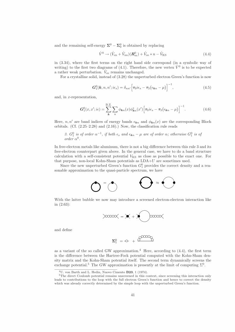
and the remaining self-energy Σ0 − Σ

00 is obtained by replacing

V 0 → (Ven + Vnn)(R0m) + Vee ∗ n− VKS (4.4)

in (3.34), where the first terms on the right hand side correspond (in a symbolic way ofwriting) to the first two diagrams of (4.1). Therefore, the new vertex V 0 is to be expecteda rather weak perturbation. Vee remains unchanged.

For a crystalline solid, instead of (3.28) the unperturbed electron Green’s function is now

G01(k, n, n

′; iǫs) = δnn′

[

τ0iǫs − τ3

(

ǫkn − µ)

]−1

, (4.5)

and, in x-representation,

G01(x, x

′; iǫ) =

B.Z.∑

k

∑

n

φkn(x)φ∗kn(x′)[

τ0iǫs − τ3

(

ǫkn − µ)

]−1

. (4.6)

Here, n, n′ are band indices of energy bands ǫkn and φkn(x) are the corresponding Blochorbitals. (Cf. (2.25–2.28) and (2.16).) Now, the classification rule reads

3. G01 is of order α−1, if both ǫs and ǫkn − µ are of order α; otherwise G0

1 is oforder α0.

In free-electron metals like aluminum, there is not a big difference between this rule 3 and itsfree-electron counterpart given above. In the general case, we have to do a band structurecalculation with a self-consistent potential VKS as close as possible to the exact one. Forthat purpose, non-local Kohn-Sham potentials as LDA+U are sometimes used.

Since the new unperturbed Green’s function G01 provides the correct density and a rea-

sonable approximation to the quasi-particle spectrum, we have

≈=

With the latter bubble we now may introduce a screened electron-electron interaction likein (2.63):

= +

and define

+=Σ01

as a variant of the so called GW approximation.4 Here, according to (4.4), the first termis the difference between the Hartree-Fock potential computed with the Kohn-Sham den-sity matrix and the Kohn-Sham potential itself. The second term dynamically screens theexchange potential.5 The GW approximation is presently at the limit of computing Σ0.

4U. von Barth and L. Hedin, Nuovo Cimento B23, 1 (1974).5The direct Coulomb potential remains unscreened in this context, since screening this interaction only

leads to contributions to the loop with the full electron Green’s function and hence to correct the densitywhich was already correctly determined by the simple loop with the unperturbed Green’s function.

41

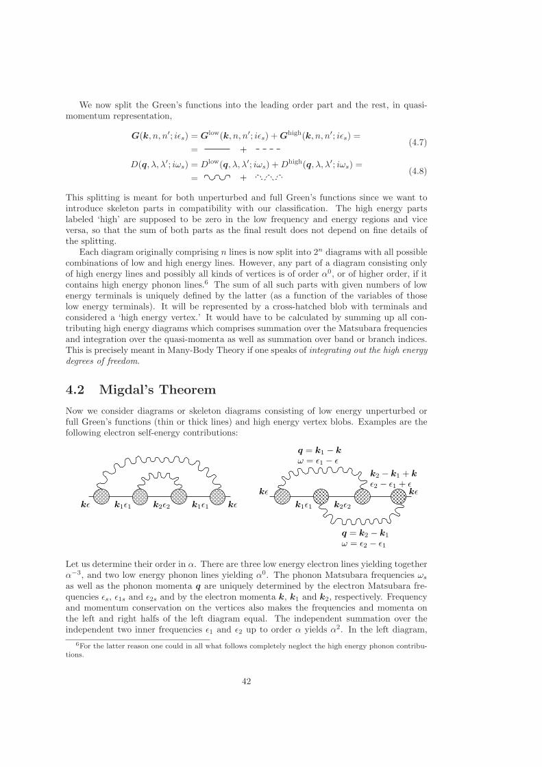
We now split the Green’s functions into the leading order part and the rest, in quasi-momentum representation,

G(k, n, n′; iǫs) = Glow(k, n, n′; iǫs) + Ghigh(k, n, n′; iǫs) =

= +(4.7)

D(q, λ, λ′; iωs) = Dlow(q, λ, λ′; iωs) +Dhigh(q, λ, λ′; iωs) =

= +(4.8)

This splitting is meant for both unperturbed and full Green’s functions since we want tointroduce skeleton parts in compatibility with our classification. The high energy partslabeled ‘high’ are supposed to be zero in the low frequency and energy regions and viceversa, so that the sum of both parts as the final result does not depend on fine details ofthe splitting.

Each diagram originally comprising n lines is now split into 2n diagrams with all possiblecombinations of low and high energy lines. However, any part of a diagram consisting onlyof high energy lines and possibly all kinds of vertices is of order α0, or of higher order, if itcontains high energy phonon lines.6 The sum of all such parts with given numbers of lowenergy terminals is uniquely defined by the latter (as a function of the variables of thoselow energy terminals). It will be represented by a cross-hatched blob with terminals andconsidered a ‘high energy vertex.’ It would have to be calculated by summing up all con-tributing high energy diagrams which comprises summation over the Matsubara frequenciesand integration over the quasi-momenta as well as summation over band or branch indices.This is precisely meant in Many-Body Theory if one speaks of integrating out the high energydegrees of freedom.

4.2 Migdal’s Theorem

Now we consider diagrams or skeleton diagrams consisting of low energy unperturbed orfull Green’s functions (thin or thick lines) and high energy vertex blobs. Examples are thefollowing electron self-energy contributions:

kǫǫ2 − ǫ1 + ǫk2 − k1 + k

kǫkǫ k1ǫ1 k2ǫ2 k1ǫ1

q = k1 − k

ω = ǫ1 − ǫ

q = k2 − k1

ω = ǫ2 − ǫ1

kǫ

k1ǫ1 k2ǫ2

Let us determine their order in α. There are three low energy electron lines yielding togetherα−3, and two low energy phonon lines yielding α0. The phonon Matsubara frequencies ωs

as well as the phonon momenta q are uniquely determined by the electron Matsubara fre-quencies ǫs, ǫ1s and ǫ2s and by the electron momenta k, k1 and k2, respectively. Frequencyand momentum conservation on the vertices also makes the frequencies and momenta onthe left and right halfs of the left diagram equal. The independent summation over theindependent two inner frequencies ǫ1 and ǫ2 up to order α yields α2. In the left diagram,

6For the latter reason one could in all what follows completely neglect the high energy phonon contribu-tions.

42

there are independent integrations over k1 and k2, each over layers of thickness ∼ α aroundthe sheets of the Fermi surface. (The thickness of the k-layer is equal to the thickness of the(ǫkn − µ)-layer divided by the Fermi velocity of the reference band structure which latteris on the high energy scale and hence ∼ α0.) Since the low energy phonon momenta areunrestricted, there is no further restriction on the electron momenta. The two k-integrationsyield another factor α2. Hence, in total from the low energy lines, the frequency summationsand the k-integrations we find the order α−3α2α2 = α for the left diagram.

The difference in the right diagram comes from the additional condition that k2−k1 +k

must also lie in an α-layer around a sheet of the Fermi surface. Hence, k2 must now be closeto the intersection of two sheets of the Fermi surface. One drawn from the origin and onedrawn from the point k1 − k. While in three and two dimensions the Fermi surface is two-and one-dimensional and that intersection is one- and zero-dimensional, respectively, in onedimension there appears no new restriction. There, if k, k1 and k2 are close to a Fermipoint, then k2 −k1 + k is either. (In particular cases which are called Fermi surface nestingthis situation may also appear in higher dimensions.) In higher than one dimension and inthe absence of nesting we find for the right diagram in total by an analogous count as abovethe order α−3α2α3 = α2. Only in one dimension or in case of nesting the same order as forthe left diagram is obtained.

In order to calculate the full electron Green’s function Glow = Glow0 ΣGlow in leading

order α−1, one needs the self-energy Σ in leading order α. The above considered diagramsare part of the skeleton diagrams

The inner phonon line of the previous left diagram is part of the inner full electron line ofthe left skeleton diagram (it contributes to the self energy of that full electron line). Thecheckered vertex on the right skeleton diagram means a full (high energy plus low energy)vertex, to which the right phonon line of the previous right diagram contributes. Migdalhas shown7 that our above findings regarding the order of such diagrams are quite general:

In higher than one dimension and in the absence of nesting, all phononic con-tributions to vertices are of higher than the leading order in α.

What about low energy electronic contributions to full vertices. Consider as an examplethe diagram

kǫ

k1 + k3 − k2

ǫ1 + ǫ3 − ǫ2

kǫ k1ǫ1 k2ǫ2

k3ǫ3

k3 + k1 − k

ǫ3 + ǫ1 − ǫ

It contributes to the right skeleton diagram above. There are four additional low energyelectron lines entering the right full vertex and yielding a contribution of order α−4. Thereare two additional frequency summations over ǫ2 and ǫ3, yielding α2. There are the corre-sponding momentum integrations over k2 and k3 running over Fermi surface layers. Both

7He proved it on the basis of Frohlich’s Hamiltonian, which in this context makes no difference.

43

momenta must, however, fulfill an additional condition which reduces both integrations tointersections of Fermi surfaces with shifted ones. These two integrations hence yield α4, andthe total order of the vertex correction is α−4α2α4 = α2. (It is easily seen that withoutthe phonon line the pure electron vertex would also be of order α2 = α−3α2α3.) By thisreasoning, the factor α−1 of each inner low energy electron line is compensated by a factorα from momentum integration, and the order of the contribution is equal to the number ofindependent new frequency summations:

In higher than one dimension and in the absence of nesting, all low energy elec-tronic contributions to vertices are of higher than the leading order in α.

In all what follows we assume an effective dimension higher than one and the absence ofnesting.

4.3 Leading Order Self-Energies

With these results, the leading order low energy electron self-energy skeleton diagrams are:

+++=Σ

(4.9)

The first contribution is the high energy electron self-energy in the static solid (Σ0 − Σ00

of Section 4.1). It is formally of order α0. This would lead to the appearance of all ordersα−n for all n > 0 in an expansion of Dyson’s equation for the low energy electron Green’sfunction (since G0 ∼ α−1 in G = G0 + G0ΣG would not be compensated by Σ ∼ α inthe second term). Hence it would completely destroy our systematics because our rule 3. ofSection 4.1 would not any more carry over to the full Green’s function. This is why it wasso important to replace the free-electron Green’s function G0 by the band structure Green’sfunction G0

1 in such a way that the remaining self-energy Σ−Σ00, although formally of order

α0, is practically small of order α in the low energy low frequency domain.The second contribution was analyzed in the preceding section, and the last two contri-

butions to Σ contain dressed four leg vertices which are indeed of order α0. However, boththe electron and the phonon loop introduce a factor α: Their frequencies and momenta areindependent from those of the terminals, and hence, by way of the analysis of the last sec-tion the electron loop introduces α−1αα, and the phonon loop introduces α0αα0, the latterfactor since the low energy phonon momentum is unrestricted.

In view of the independence of the frequencies and momenta of the loops one could thinkthat those last two contributions to Σ have a weak frequency and momentum dependence,changing only on the large energy scale like the first contribution. This is indeed the casefor the last diagram, the last but one, however, will develop an anomalous part in thesuperconducting state since the full Green’s function of the electron loop will develop sucha part. Hence, the essential low energy electronic self-energy contributions are the middletwo of (4.9).

The leading order low energy phonon self-energy consists only of the high energy blob oforder α0:

=Π

(4.10)

This is consistent with our systematics, since Dlow0 ∼ α0, and hence Dyson’s equation

preserves this order for Dlow. Hence, the low energy electron Green’s function does notenter the phonon problem to leading order. It is completely determined by the high energy

44

electronic structure and hence by band structure theory. The superconducting state onlyweakly influences the phonon spectrum.

Since the high energy blob of (4.10) has a frequency and energy dependence of the highenergy scale, to leading order this dependence can be neglected in the low energy range,hence (4.10) may be approximated by the adiabatic expression (in the representation of(3.29))

Π(lλ, l′λ′; 0) =∂2E0

∂ulλ∂ul′λ′

∣

∣

∣

∣

u=0

(4.11)

where E0 is the total energy of the normal electronic ground state in a static assembly ofnuclei at positions with coordinates R0

lλ + ulλ. Note that due to (3.22, 3.23) each diagramwith a phononic terminal is obtained from a corresponding diagram without that terminalby differentiation with respect to the nuclear positions.

Multiplication of the force constant matrix elements on the right hand side of (4.11) with1/√MλMλ′ and diagonalization of the resulting matrix yields

Π(lλ, l′λ′; 0) =1

M

∑

qκ

eiq·R0

l eλ(qκ)ω2qκe

∗λ′(qκ)e−iq·R0

l′ , (4.12)

where M is the number of unit cells as previously and the orthogonal polarization vectors eare complete and normalized in such a way that:

1

M

∑

qκ

eiq·R0

l eλ(qκ)e∗λ′(qκ)e−iq·R0

l′ = δll′δλλ′Mλ (4.13)

with the nuclear masses Mλ. Hence, from Dyson’s equation in the form D−1 = D−10 − Π

one finds readily

D(lλ, l′λ′; iωs) = − 1

M

∑

qκ

eiq·R0

l eλ(qκ)1

ω2s + ω2

qκ

e∗λ′(qκ)e−iq·R0

l′ (4.14)

or

D(q, λ, λ′; iωs) = −∑

κ

eλ(qκ)1

ω2s + ω2

qκ

e∗λ′(qκ). (4.15)

If one is interested in the effect of the superconducting state on the phonon frequencies,one can of course calculate a next correction term to Π of a form analogous to the thirddiagram in (4.9).

The same type of consideration as in (4.11) immediately shows that every tadpole partof diagram with a phononic tail is exactly zero in a harmonic crystal:

=

∂E0

∂ulλ

∣

∣

∣

∣

u=0

= 0.(4.16)

Here, the checkered blob means again a full (high plus low energy) skeleton vertex, whichat variance to (4.10) is correctly to all orders in α equal to the first derivative of the totalenergy with respect to the nuclear position. The vanishing of all those first derivativesjust defines the nuclear equilibrium positions relative to which the adiabatic and harmonicphonons are defined. For that reason we did not include tadpole parts with phononic tailsinto our analysis of orders of α (where they would not fit in, if they were non-zero). Ina harmonic crystal, 〈Rm〉 = R0

m holds independent on temperature, there is no thermalexpansion. Anharmonic corrections change this behavior and also correct (4.16).

45

Chapter 5

The Low Energy Equations

In the last chapter, two high energy problems have been separated from the low energyproblem of superconductivity (and of low energy transport in general): the problem (4.1–4.6) of the self-consistent electronic structure of the solid without lattice displacements andthe problem (4.11–4.15) of the adiabatic lattice dynamics of the solid. Both problems need acareful treatment of self-consistent screening of the Coulomb interaction and hence a carefulcalculation of the electronic density. Density functional methods provide nowadays the mostpowerful approach to both problems and allow effectively to solve them with the neededaccuracy.

The remaining part of the electron self-energy, Σ0 − Σ

00, which relates the full high

energy Green’s function, G0, to the unperturbed Green’s function, G01, of non-interacting

band states, may be addressed by GW methods. For the sake of brevity, this remaining partof the self-energy is denoted by Σ

01 in the following. Since it is small, it may be considered

to be of the low energy scale in magnitude but vary on the high energy scale as demanded.This lets us write

Σ01(r, r

′; iǫs) = τ3Σ01(r, r

′; 0) + τ0Σ01′(r, r′; 0) iǫs. (5.1)

as the Taylor expansion of the frequency dependence of Σ01 to linear order. From (3.16) one

can see that not only the sign of the Nambu component G22 is reversed compared to G11

but also the sign of the frequency argument. This must also hold true for Σ0, whence the

first order Taylor term is ∼ τ0. In a normal metal, the imaginary part of Σ0 is ∼ ǫ2, henceΣ0

0 and Σ01 are real (and symmetric as integral operators).

As for the adiabatic lattice dynamics calculated with density functional methods, itnowadays agrees typically within five to ten percent with the experimental phonon spectra.

Given these results and the high energy vertices, the problem of superconductivity re-duces to the solution of the closed non-linear equation system

∫

d3r1

[

τ0iǫsa−1(r, r1)−τ3H

0(r, r1)−Σep1 (r, r1; iǫs)−Σ

ee1 (r, r1; iǫs)

]

Glow(r1, r′; iǫs) =

= τ0δ(r − r′) (5.2)

which is Dyson’s equation for Glow to leading order with the self-energy contributions of thefirst three diagrams of (4.9). H0 consists of HKS and Σ0

1, and a−1 contains Σ01′. Eq. (5.2)

is non-linear since Σep1 and Σ

ee1 depend on Glow.

46

5.1 The Quasi-Particle Renormalization

The first term of (5.2) contains the linear Taylor term of (5.1). Like in (2.62) it leads to arenormalization of the quasi-particle amplitude,

a(r, r′) =[

δ(r − r′) − Σ01′(r, r′; 0)

]−1 ≈ δ(r − r′) + Σ01′(r, r′; 0). (5.3)

(The exponent −1 means the kernel of the inverse integral operator.) This so called Coulombrenormalization factor barely ever has really been calculated for a real band structure.1 Itcould be addressed by GW methods as mentioned above. In normal metals, |Σ0

1′| is of the

order of 0.1 to 0.3, and hence only Σ01′2

is small of order α. (In (5.1), although Σ01 ∼ α, Σ0

1′

may be of order α0, since in the low frequency domain ǫs is of order α.)In the standard approach the Coulomb renormalization factor is considered by renor-

malizing all quantities entering (5.2):

g = τ3a−1/2 ∗ Glow ∗ a−1/2, (5.4)

h0 = a1/2 ∗H0 ∗ a1/2, (5.5)

σep = a1/2 ∗ Σep1 ∗ a1/2τ3, (5.6)

σee = a1/2 ∗ Σee1 ∗ a1/2τ3, (5.7)

where for the sake of brevity a notation of integral operators was used,

a±1/2 ≈ 1 ± 1

2Σ0

1′, (5.8)

and the star means the operation

(a ∗ b)(r, r′) =

∫

d3r1a(r, r1)b(r1, r′). (5.9)

(The factors τ3 in (5.4–5.7) are just convention to reduce the number of factors τ3 in thefollowing relations.) Dyson’s equation (5.2) renormalizes to

[

τ3iǫs − τ0h0 − σee − σep

]

∗ g = 1. (5.10)

The Hamiltonian H0 for the high energy quasi-particle band structure was

H0(r, r′) = HKS(r, r′) + Σ01(r, r

′; 0) (5.11)

with HKS from (4.3). From its renormalized form an effective quasi-particle potential

v0 = h0 − (t− µ) = VKS + Σ01 +

1

2

[

H0, Σ01′ ]

+

(5.12)

may be extracted, which is meaningful for low electron energies (that is close to the Fermisurface) since (5.1) was meaningful in that domain. It is related to the quasi-particle Green’sfunction g (which in the normal state has a spectral amplitude equal to one at the quasi-particle pole and yields a quasi-particle quasi-momentum distribution which jumps fromunity to zero at the Fermi surface). The quasi-particle Green’s function g on the other handis related to the true electron Green’s function G via (5.4) in the low energy domain wherewe still neglect ImΣ ∼ α2. In practical calculations v0 is often approximated by VKS, whileΣ0

1′should not be neglected in (5.4, 5.6, 5.7).

1It has been calculated by many authors for the homogeneous electron liquid or for model systems.

47

5.2 The Electron-Phonon Self-Energy

The potential v0 is also intimately related to the (high energy) electron-phonon vertexentering the second diagram of (4.9). As was already explained in connection with (4.11),a diagram with a phonon leg is obtained from the corresponding diagram without that legby differentiation with respect to the nuclear positions. In the considered case, the electron-phonon vertex denoted by Γep(r, r′|lλ) is obtained by differentiating the two leg electronvertex Σ0(r, r′; 0) of (4.1):

Γep(r, r′|lλ) =∂Σ0(r, r′; 0)

∂ulλ

∣

∣

∣

∣

u=0

. (5.13)

(Since we need the vertices only to zeroth order and in the low frequency range of the legs,Σ0 may be taken for ǫs → 0 here.) In accordance with the previous section we define arenormalized electron-phonon vertex as

γep = a1/2 ∗ Γep ∗ a1/2. (5.14)

With the help of the Feynman rules of Section 2.6, the electron-phonon self-energy diagram(second diagram of (4.9)) is translated into

Σep(r, r′; iǫs) = −

∫

d3r1d3r′1

∑

lλ,l′λ′

1

β

∑

s′

Γep(r, r1|lλ)τ3Glow(r1, r

′1; iǫs − iωs′)τ3Γ

ep(r′1, r

′|l′λ′)D(lλ, l′λ′; iωs′).

(5.15)

(The two factors 1/β attached with Glow and D are canceled against the two factors βattached with the two vertices. Since a self-energy diagram has external structure like aGreen’s function with two vertices, it is translated into −βΣ. Additionally, like H0 in (5.2),each pair of electron legs of electron-electron and electron-phonon vertices gets a factor τ3.)

Substituting (5.15) with the renormalized quantities (5.4–5.7, 5.14) yields finally

σep(r, r′; iǫs) = −∫

d3r1d3r′1

∑

lλ,l′λ′

1

β

∑

s′

γep(r, r1|lλ)g(r1, r′1; iǫs − iωs′)γep(r′

1, r′|l′λ′)D(lλ, l′λ′; iωs′).

(5.16)

The electron-phonon vertex γep is obtained from (5.14) and (5.13):

γep = a1/2 ∗ ∂Σ0

∂u∗ a1/2 = a1/2 ∗ ∂H

0

∂u∗ a1/2 =

= a1/2 ∗[

∂

∂ua−1/2 ∗ h0 ∗ a−1/2

]

∗ a1/2 =∂h0

∂u− 1

2

[

a−1 ∗ ∂a∂u

∗ h0 + h0 ∗ ∂a∂u

∗ a−1

]

.

(5.17)

Since h0 ∼ α in the low energy domain while vertices are generally ∼ α0, the terms in squarebrackets may be neglected, and the final leading order result is

γep(r, r′|lλ) =∂v0(r, r′)

∂ulλ

∣

∣

∣

∣

u=0

. (5.18)

This important result says that the renormalized electron-phonon vertex is obtained as thechange of the quasi-particle crystal potential for a static displacement of the nuclear positionout of equilibrium. It may readily be calculated like v0 itself by means of the same densityfunctional approach, possibly corrected with GW methods.

48

5.3 The Electron-Electron Self-Energy

The third diagram of (4.9) translates into

Σee(r, r′; iǫs) = −

∫

d3r1d3r′1

1

β

∑

s′

Γee(r, r′, r1, r′1; iǫs, iǫs′)τ3G

low(r1, r′1; iǫs′)τ3 (5.19)

(This relation also defines which sign and β factors are attached with Γee.)The Nambu structure of this diagram is

−

−

=

For the diagonal elements, the same holds true what was said in Section 4.3 about thefourth diagram of (4.9). They need not be considered further and we may concentrate onthe off-diagonal diagrams in the sequel.

Even if the normal metallic state is not spin polarized, the exchange part of the electron-electron interaction and hence also Γee depends on the spin of the electrons. For the caseof singlet pairing considered throughout this text, the spin structure of G and Σ was finallydetermined in (3.19). In (5.19), Γee has to be taken in accordance with that spin structure.Clearly, this is different for instance for singlet and triplet pairing, respectively.

Before going into the details, we also observe that again the frequency dependence ofthe vertex Γee may be neglected to leading order for the same reason as in all previousconsiderations of that point, and the vertex may be taken at zero frequencies (in the senseof analytic continuation; zero itself is not an electron Matsubara frequency). Moreover, itmay be renormalized for each electron leg:

γee(r, r′, r1, r′1) =

∫

d3r2d3r′2d

3r3d3r′3a

1/2(r, r2)a1/2(r′, r′

2)Γee(r2, r

′2, r3, r

′3; 0, 0)a1/2(r3, r1)a

1/2(r′3, r

′1).

(5.20)

This reduces (5.19) to

σee(r, r′) = −∫

d3r1d3r′1

1

β

∑

s′

γee(r, r′, r1, r′1)g(r1, r

′1; iǫs′), (5.21)

of which the Nambu off-diagonal matrix elements matter only. Like the vertex, the electron-electron self-energy is to leading order frequency independent.

5.4 Bloch Function Representation on the

Fermi Surface

We now introduce a representation in terms of low energy quasi-electron Bloch states, thatis, eigenstates of the (Hermitian) Hamiltonian h0 with the kernel

h0(r, r′) =

[

−1

2

∂2

∂r2− µ

]

δ(r − r′) + v0(r, r′) (5.22)

49

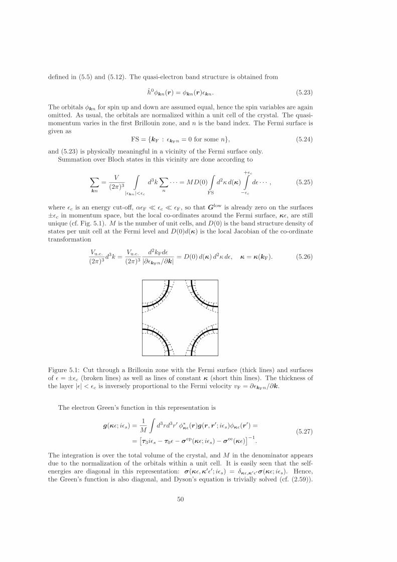
defined in (5.5) and (5.12). The quasi-electron band structure is obtained from

h0φkn(r) = φkn(r)ǫkn. (5.23)

The orbitals φkn for spin up and down are assumed equal, hence the spin variables are againomitted. As usual, the orbitals are normalized within a unit cell of the crystal. The quasi-momentum varies in the first Brillouin zone, and n is the band index. The Fermi surface isgiven as

FS = kF : ǫkFn = 0 for some n, (5.24)

and (5.23) is physically meaningful in a vicinity of the Fermi surface only.Summation over Bloch states in this vicinity are done according to

∑

kn

=V

(2π)3

∫

|ǫkn|<ǫc

d3k∑

n

· · · = MD(0)

∫

FS

d2κ d(κ)

+ǫc∫

−ǫc

dǫ · · · , (5.25)

where ǫc is an energy cut-off, αǫF ≪ ǫc ≪ ǫF, so that Glow is already zero on the surfaces±ǫc in momentum space, but the local co-ordinates around the Fermi surface, κǫ, are stillunique (cf. Fig. 5.1). M is the number of unit cells, and D(0) is the band structure density ofstates per unit cell at the Fermi level and D(0)d(κ) is the local Jacobian of the co-ordinatetransformation

Vu.c.

(2π)3d3k =

Vu.c.

(2π)3d2kFdǫ

|∂ǫkFn/∂k| = D(0) d(κ) d2κ dǫ, κ = κ(kF). (5.26)

Figure 5.1: Cut through a Brillouin zone with the Fermi surface (thick lines) and surfacesof ǫ = ±ǫc (broken lines) as well as lines of constant κ (short thin lines). The thickness ofthe layer |ǫ| < ǫc is inversely proportional to the Fermi velocity vF = ∂ǫkFn/∂k.

The electron Green’s function in this representation is

g(κǫ; iǫs) =1

M

∫

d3rd3r′ φ∗κǫ(r)g(r, r′; iǫs)φκǫ(r′) =

=[

τ3iǫs − τ0ǫ− σep(κǫ; iǫs) − σee(κǫ)]−1

.

(5.27)

The integration is over the total volume of the crystal, and M in the denominator appearsdue to the normalization of the orbitals within a unit cell. It is easily seen that the self-energies are diagonal in this representation: σ(κǫ,κ′ǫ′; iǫs) = δκǫ,κ′ǫ′σ(κǫ; iǫs). Hence,the Green’s function is also diagonal, and Dyson’s equation is trivially solved (cf. (2.59)).

50

Indeed, due to the conservation of the total quasi-momentum at every vertex, self-energiesand Green’s functions are k-diagonal. However, in the considered low energy domain theband index n is uniquely determined by k, and kn-diagonal is the same as κǫ-diagonal.

Eq. (5.16) now reads

σep(κǫ; iǫs) = −∑

lλ,l′λ′

1

β

∑

s′

D(0)

M

∫

FS

d2κ′ d(κ′)

∫

dǫ′

〈φκǫ|γeplλ |φκ′ǫ′〉g(κ′ǫ′; iǫs − iωs′)〈φκ′ǫ′ |γep

l′λ′ |φκǫ〉D(lλ, l′λ′; iωs′) ≈

≈−∑

lλ,l′λ′

1

β

∑

s′

D(0)

M

∫

FS

d2κ′ d(κ′)

〈φκ0|γeplλ |φκ′0〉

∫

dǫ′ g(κ′ǫ′; iǫs − iωs′) 〈φκ′0|γepl′λ′ |φκ0〉D(lλ, l′λ′; iωs′).

(5.28)

Since all ǫ are small and the matrix element of the vertex (5.18) may depend on the energyof the orbitals on the high energy scale only, again to leading order all energy dependencesin the vertex may be neglected. Then, the self-energy does not depend on ǫ any more andonly depends on the energy-integrated Green’s function2

g(κ; iǫs) =

∫

dǫ g(κǫ; iǫs), (5.29)

which is a function on the Fermi surface only. The theory of superconductivity is thenexpressed in terms of functions on the Fermi surface.

With

Iep(κ,κ′|lλ) = 〈φκ0|∂v0

∂ulλ|φκ′0〉 (5.30)

and

λ(κ,κ′; iωs) = −D(0)

M

∑

lλ,l′λ′

Iep(κ,κ′|lλ)D(lλ, l′λ′; iωs)Iep(κ′,κ|l′λ′) (5.31)

the electron-phonon self-energy is

σep(κ; iǫs) =1

β

∑

s′

∫

d2κ′ d(κ′)λ(κ,κ′; iωs′) g(κ′; iǫs − iωs′). (5.32)

This quantity is often averaged over the Fermi surface. Additionally one introduces a phononspectral function B(lλ, l′λ′;ω) according to

D(lλ, l′λ′; iωs) = −2

∞∫

0

dωB(lλ, l′λ′;ω)ω

ω2s + ω2

(5.33)

and a spectral density α2F (ω) of the averaged λ-function:

λ(iωs) =

∫

FS

d2κd2κ′ d(κ)d(κ′)λ(κ,κ′; iωs) = 2

∞∫

0

dω α2F (ω)ω

ω2s + ω2

, (5.34)

2G. Eilenberger, Z. Phys. 214, 195 (1968); A. I. Larkin and Yu. N. Ovchinnikov, Sov. Phys.-JETP 28,1200 (1969).

51

α2F (ω) =D(0)

∫

FS

d2κd2κ′ d(κ)d(κ′)

1

M

∑

lλ,l′λ′

Iep(κ,κ′|lλ)B(lλ, l′λ′;ω)Iep(κ′,κ|l′λ′).(5.35)

The electron-phonon mass enhancement is λ = λ(0).Finally, the matrix elements of the electron-electron vertex are

µ∗(κ,κ′) =D(0)

M〈φκ0|〈φ−κ0|γee|φκ′0〉|φ−κ′0〉, (5.36)

where φ−κ0 is the time reversal of the state φκ0, that is, the state with reversed quasi-momentum k (and reversed spin). The Nambu non-diagonal electron-electron self-energyon the Fermi surface reads

[σee(κ)]i6=j = −∫

d2κ′ d(κ′)µ∗(κ,κ′)1

β

|ǫs′|<ǫc∑

s′

[g(κ′; iǫs′)]i6=j . (5.37)

The frequency cut-off has again been put to a value where the low energy Green’s functionshould have converged so that the final results of the theory to leading order do not dependon this cut-off. For the electron-electron pseudopotential µ∗ also a Fermi surface average

µ∗ =

∫

d2κd2κ′ d(κ)d(κ′)µ∗(κ,κ′) (5.38)

is introduced for later use.With (5.32) and (5.37), the energy integrated Green’s function (5.29) is now

g(κ; iǫs) =

∫

dǫ[

τ3iǫs − τ0ǫ− σep(κ; iǫs) − σee(κ)]−1

. (5.39)

From the integral

+a∫

−a

dx1

z − x= Ln(z − a) − Ln(z + a) = ln

∣

∣

∣

z − a

z + a

∣

∣

∣+ iArg

(z − a

z + a

)

≈

≈− 4Re z

a− i(

π − 2Im z

a

)

sign(Im z) ≈ −iπ sign(Im z),

(5.40)

where z is complex and x is real, we see that for a large enough cut-off energy ǫc (5.39) hasto leading order a meaning independent of the cut-off.

Now the general electron-phonon theory of superconductivity for normal metals withoutFermi surface nesting is reduced to Eliashberg’s equations (5.39), (5.32) and (5.37), the lowenergy equations of the microscopic theory for arbitrarily strong coupling.

52

Chapter 6

Strong Coupling Theory of the

Transition Temperature

In the introduction to Chapter 3 we found that the signature of the superconducting stateis the appearance of non-zero anomalous Green’s functions involving the pair operators,that is, the appearance of Nambu off-diagonal components of the Green’s function. Abovethe transition temperature Tc, in the normal conducting state, those components are zero.Since in the absence of an external magnetic field the transition into the superconductingstate is a second order phase transition, those components veer off continously to non-zerovalues below Tc. Hence, close to Tc the off-diagonal components are small, and Eliashberg’sequations (5.39), (5.32) and (5.37) may be linearized in those components. This is why thetheory of the transition temperature for given quasi-particle band structure, λ(s, s′; iωs) andµ∗(s, s′) is the simplest part of the microscopic theory of superconductivity.

In the BCS theory,1 which is correct in the weak coupling limit, that is, for Tc ≪ ωph inaddition to the small parameter α, Tc is obtained from the solubility condition of a simplegap equation to be

Tc =2γ

πωph exp

− 1

gBCSD(0)

(6.1)

with γ = eC where C is Euler’s constant, 2γ/π ≈ 1.13. Here, ωph is the relevant phononenergy determining the cut-off for the BCS attraction with coupling constant gBCS. Hence,Tc is known once one has calculated gBCS, ωph and D(0) from a microscopic theory with theabove mentioned ingredients. However, calculating gBCS is not really simpler than the directsolution of the strong coupling Tc-equations as described below, and there is no reason anymore to use one of the many semi-empirical derivates of (6.1) found in the literature.

6.1 Linearization of Eliashberg’s Equations

We continue to consider singlet pairing in the absence of magnetic fields or spin dependentdirect interactions. Hence the spin structure of the Nambu Green’s function and self-energyis given by (3.19). We continue to omit the factors σ0 and σ2 since they are automaticallycorrectly replaced in Nambu matrix multiplications:

(

σ0 σ2

σ2 σ0

) (

σ0 σ2

σ2 σ0

)

= 2

(

σ0 σ2

σ2 σ0

)

. (6.2)

1J. Bardeen, L. Cooper and J. R. Schrieffer, Phys. Rev. 108, 1175 (1957); G. Rickayzen, in: R. D. Parks(ed.), Superconductivity, vol. 1, p. 51, Dekker, New York 1969.

53

Apart from these Pauli spin factors, traditionally the Green’s function is expressed as2

g(κ; iǫs) =

(

g(κ; iǫs) if(κ; iǫs)if∗(−κ; iǫs) g∗(−κ; iǫs)

)

(6.3)

and the self-energy as

σep(κ; iǫs) + σee(κ) =

(

i(ǫs − ǫs(κ)) iφs(κ)iφ∗s(κ) −i(ǫs − ǫs(κ))

)

. (6.4)

We insert (6.4) into (5.39), invert the 2 × 2 matrix according to

(

a bc d

)−1

=1

ad− bc

(

d −b−c a

)

, (6.5)

and obtain

g(κ; iǫs) =

∫

dǫ−ǫ− iǫs(κ)

(−ǫ+ iǫs(κ))(−ǫ− iǫs(κ)) + φs(κ)φ∗s(κ)(6.6)

and

if(κ; iǫs) =

∫

dǫiφs(κ)

(−ǫ+ iǫs(κ))(−ǫ− iǫs(κ)) + φs(κ)φ∗s(κ). (6.7)

Linearizing these relations with respect to the off-diagonal matrix elements means neglectingφφ∗ in the denominators. Then, the integrations are elementary with the results

g(κ; iǫs) = −iπ sign(ǫs(κ)), f(κ; iǫs) = πφs(κ)

|ǫs(κ)| . (6.8)

(The first integral is a principal value integral, cf. (5.40), the second one can for instance bedone by contour integration.)

Below we will see that sign(ǫs(κ)) = sign ǫs, hence we can make this replacement. If wenow insert these results into (5.32) and (5.37) and compare to (6.4), we obtain

i(ǫs − ǫs(κ)) =1

βc

∑

s′

∫

d2κ′ d(κ′)λ(κ,κ′; iωs′) (−iπ sign(ǫs − ωs′)), (6.9)

iφs(κ) =1

βc

∑

s′

∫

d2κ′ d(κ′)λ(κ,κ′; i(ǫs − ǫs′)) iπφs′(κ′)

|ǫs′(κ′)| −

−∫

d2κ′ d(κ′)µ∗(κ,κ′)1

βc

|ǫs′|<ǫc∑

s′

iπφs′(κ′)

|ǫs′(κ′)| .(6.10)

Here, βc = 1/Tc since the linearized relations are valid close to the transition temperature,Tc, only. In the first term of the last relation we have changed the summation over ωs′ intoa summation over ǫs′ , where ǫs′ = ǫs − ωs′ . This summation may again be cut off at alarge frequency ǫc without specifying the (earlier) cut off of the low energy Green’s functionf(κ′; iǫs′) because the factor λ(iωs′) ∼ D(iωs′) ∼ ω−2

s′ provides a sufficient convergencyfactor.

2Compare (3.16) with (2.35) and (2.7). Then, from (5.27) with φ−κǫ(r, s) = φ∗κǫ(r,−s), transposition

of x with x′ replaces κ with −κ in the spin singlet Green’s function, and multiplication with τ3 in (5.4)removes the factors −1 in the lower line of the Nambu matrix. For the off-diagonal elements, (6.3) is anansatz which fixes the phase of the superconducting order parameter to be zero.

In view of (5.32) and (5.37), σ has the same structure as g, only it does not depend on the sign of κ dueto time reversion symmetry implying λ(−κ,−κ′) = λ(κ, κ′), µ∗(−κ,−κ′) = µ∗(κ, κ′).

54

Consider first (6.9) and realize that λ, like D, is an even function of ωs′ . Hence, due tothe presence of the sign factor, in the s′-summation all items for positive ωs′ > |ǫs| cancelall items for negative ωs′ < −|ǫs|. Between these limits, the sign of ǫs − ωs′ is equal to thesign of ǫs, and the final result is

ǫs(κ) = ǫs + sign(ǫs)π

βc

|ωs′|<|ǫs|∑

s′

∫

d2κ′ d(κ′)λ(κ,κ′; iωs′). (6.11)

Since from (2.33) (π/β)∑|ω

s′|<|ǫs|

s′ 1 ≈ |ǫs|, we see that the normal component of theelectron-phonon self-energy is proportional to λ and proportional to ǫs. Eq. (6.11) holdsalso for ωph > β−1 > β−1

c in the normal state where φs = 0 = f . This results inG−1 = iǫs(1 + λ) − ǫkn which for the quasi-particle pole means ǫkn = ǫkn/(1 + λ), thewell known result for the normal state at low temperatures. Moreover, since λ was definedin (5.31) to be positive at imaginary frequencies (D is negative definite at imaginary fre-quencies, cf. (4.14)), it follows from (6.11) that indeed sign(ǫs(κ)) = sign(ǫs), consistentwith the assumption in (6.9).

The determination of the normal component of the low energy electron self-energy via(6.11) reduces now to the computation of a finite number of Fermi surface integrals over λ.

6.2 The Tc Formula

Having computed the normal component of the self-energy via (6.11) and (5.30, 5.31), theintegral equation (6.10) for the anomalous component φs(κ) may be considered. (The lessrigorous treatment of µ∗ from (5.36) is postponed to Section 6.4.) We symmetrize (6.10) byintroducing a new function

ψs(κ) =φs(κ)

√

d(κ)|ǫs(κ)|(6.12)

and the kernel

K(κ, s;κ′, s′) =

√

πd(κ)

βc|ǫs(κ)|[

λ(κ,κ′; i(ǫs − ǫs′)) − µ∗(κ,κ′)]

√

πd(κ′)

βc|ǫs′(κ′)| . (6.13)

ǫs = (2s+ 1)π/βc. (6.14)

Then, (6.10) reads

ψs(κ) =

|ǫs′|<ǫc∑

s′

∫

d2κK(κ, s;κ′, s′)ψs′(κ′). (6.15)

This equation may have a non-zero solution, if the operator defined by the kernel K has aneigenvalue equal to unity.

The integral operator K is defined by a finite sum and an integral over a finite surfaceover the Hermitian kernel K which is bounded and continuous as a function of two variablesκ and κ′ on the Fermi surface. Hence K is compact and self-adjoint, and due to the Hilbert-Schmidt theorem it has a bounded sequence of eigenvalues ki which cluster at k = 0.

In (6.11), the number of items in the sum is ∼ βc/π. Since λ(iω) converges to a non-zerovalue for ω → 0, those items become equal for low ωs, and the temperature dependence ofthe sum is canceled by the prefactor: The normal component of the self-energy and ǫ fora given fixed ǫ is nearly temperature independent at low temperatures. Consequently, thesquare roots in (6.13) and hence K itself are again nearly temperature independent, and thesummation in (6.15) introduces a factor βc/π into the norm of K.

55

The operator and hence its spectrum is tuned with this prefactor βc/π. For Tc → ∞ itis tuned down to zero. Hence, if we lower the temperature, there may be a highest value Tc

at which the largest eigenvalue of K becomes unity. This is the superconducting transitiontemperature, since above it the only solution for ψs(κ) and hence for φs(κ) is zero. (Belowthis temperature, on the one hand we obtain a discrete sequence of temperatures for whicheigenvalues of K pass through unity and hence at which there are non-zero solutions, and onthe other hand all those solutions may have an arbitrary amplitude. Both facts are artificalaftereffects of our linearization. Non-linear corrections determine the amplitude of φs(κ)and enable nontrivial solutions of the equations (5.39), (5.32) and (5.37) for all T < Tc: Asφs(κ) is tuned up the temperature of the solution shifts downward.)

For a practical calculation in the general case, one would introduce a set of orthogonalbasis functions on the Fermi surface and expand ψs(κ) and K in this basis. Appropriatebasis functions are the so called Fermi surface harmonics. The kernel K has the symmetryof the Fermi surface, the point symmetry of the reciprocal lattice, and the solution ψs(κ)of this linear problem may always be chosen to have the same symmetry. Like the kernelK, the eigenfunction to the highest eigenvalue will have no nodes on the Fermi surface:Electron-phonon coupling leads normally to s-wave or extended s-wave pairing. (The lattermeans that, although not constant on the Fermi surface, ψs(κ) has no nodes.) It is clearthat rapid basis convergence is expected, and (6.15) is transformed into a purely algebraicmatrix problem with a not to high dimension which can easily be solved on a PC withstandard software. In most cases the largest eigenvalue is well separated from the absolutevalues of all other eigenvalues of K (which are all smaller). Then, the simple von Misesiterations are efficient to solve the eigenvalue problem for this largest eigenvalue.

The condition for this formulation of the theory in Bloch wave representation is thatthe energy width of a quasi-particle κ-state is small compared to the energy scale of thesuperconducting coupling. This is the clean limit in which the Bloch electron mean freepath is large compared to the coherence length of the pair correlation for T = 0.

6.3 The Dirty Limit

If there is impurity scattering, then κ is not conserved any more. For strong impurityscattering the Bloch function representation looses its physical relevance. In this dirtylimit we return to the Hamiltonian (5.22) and include the impurity potential into v0. Thestationary eigenstates φν(r),

h0φν(r) = φν(r)ǫν , (6.16)

are again to be considered in the low energy range only. We denote with φ−ν the timereversal of the state φν (that is the complex conjugated and spin reversed orbital) and haveto consider the analogue of (3.4) for pairs of mutually time reversed states.

Instead of (5.30, 5.31) we now have

λν,ν′;ν1,ν′

1(iωs) =

∑

lλ,l′λ′

〈ν| ∂v0

∂ulλ|ν1〉D(lλ, l′λ′; iωs)〈ν′1|

∂v0

∂ul′λ′

|ν′〉. (6.17)

The functions φν(r) have phases randomly changing from atom position to atom position,which in particular are not correlated to the phases contained in D. Products φ∗νφν′ haveagain random phases and the average of λν,ν′;ν1,ν′

1(iωs) over ν′ will essentially not depend

on ν′1 any more. The average over ν′ and ν1,

λ(iωs) = λν,ν′;ν1,ν′

1(iωs)

ν′ν1

, (6.18)

is a function of ωs only.

56

Instead of (5.32) we have

σepν,ν′(iǫs) =

1

β

∑

s′

∑

ν1,ν′

1

λν,ν′;ν1,ν′

1(iωs)gν1,ν′

1(iǫs − iωs′), (6.19)

wheregν,ν′(iǫs) = 〈ν|g(r, r′; iǫs)|ν′〉 (6.20)

averaged over ν′ keeps only a dependence on ǫν :

g(ǫν ; iǫs) = gν,ν′(iǫs)ν′

, g(iǫs) =

∫

dǫ g(ǫ; iǫs). (6.21)

If now (6.19) is averaged over ν′, then the summation over ν′1 only averages gν1,ν′

1, and after

this the summation over ν1 eventually averages λ:

σep(iǫs) = σepν,ν′(iǫs)

ν′

=1

β

∑

s′

λ(iωs)g(iǫs) (6.22)

Finally, instead of (5.36, 5.37) we have

[

σee]

i6=j= −µ

∗

β

|ǫs′|<ǫc∑

s′

[

g(iǫs′)]

i6=j(6.23)

where µ∗ is the average over the analogue of (5.36).Now, (5.39) is replaced by

∑

ν′

[

(

τ3iǫs − τ0ǫν)

δνν′ − σepνν′(iǫs) − σee

νν′

]

gν′ν′′(iǫs) = τ0δνν′′ . (6.24)

Averaging this relation over ν′′ yields

[

τ3iǫs − τ0ǫ− σep(iǫs) − σee]

g(ǫ; iǫs) = τ0. (6.25)

In the dirty limit, (6.25), (6.22) and (6.23) are the analogues to Eliashberg’s equations (5.39),(5.32) and (5.37). They have precisely the same structure except that averaged quantitiesfigure and there is no κ-dependence. This holds obviously also true for the solutions whichread

ǫs − ǫs + sign(ǫs)π

βc

|ωs′|<|ǫs|∑

s′

λ(iωs′), (6.26)

φs =π

βc

|ǫs′|<ǫc∑

s′

(

λ(iǫs − iǫs′) − µ∗) φs′

|ǫs′ | . (6.27)

The latter equation may be written as

ψs =

|ǫs′|<ǫc∑

s′

Kss′ψs′ , ψs =φs√

|ǫs|(6.28)

with the obvious meaning of Kss′ . This Tc-equation is solved in the same manner as (6.15),only it is even much simpler.

This analysis shows that non-magnetic impurities (we used spin singlet pairing conditionsand did not introduce spin flip scattering) do not suppress superconductivity. It does,

57

however, not really provide a computational approach to the averaged coupling terms λ(iǫs)and µ∗. If the electron mean free path is small compared to the coherence length (which is thecondition for the dirty limit) but still large compared to interatomic distances, then Blochfunctions are not a bad starting point to describe the electronic states, and the averages(5.34) and (5.38) may be used in the above relations. This is the case for which most strongcoupling calculations of Tc in the literature have been done.

6.4 The Cut-Off Frequency

The Green’s function (6.3) is the low energy low frequency Green’s function according tothe splitting (4.7). It should die away somewhere between the characteristic phonon energy,the Debye energy ωD say, and well below the Fermi energy. The solution (6.8) of the lin-earized Eliashberg equations does not automatically provide this behavior for the frequencydependence.

For the Nambu diagonal component g(iǫs) this is not a problem. Due to the dependenceof λ on ω2

s only, first of all the s′-sum of (6.9) is cut off at |ǫs| independently of the actualform of damping of g(iǫs) for large ǫs. Moreover, since λ ∼ ω−2

s for ωs ≫ ωD, this sumconverges towards a constant for large |ǫs|, where this constant is determined by the lowfrequency part of g(iǫs) only.

The same decay of λ(iω) provides a decay of the λ-contribution to the kernel K of(6.13) or of (6.28) away from the diagonal. Together with the ǫ−1

s -decay along the diagonalthis provides sufficient convergency again to render results independent of the actual highfrequency damping of the Green’s function. This is, however, not the case for the µ∗-contribution since it does not decay off the diagonal of K. To get rid of an unphysicaldependence of the results on the frequency cut-off, ǫc, through this contribution to K, oneintroduces a compensating ǫc-dependence of µ∗ in the following way:

Since the correction term in (6.11) converges to a constant, one has ǫs/ǫs → 1 for large|ǫs| and hence, from (6.8), [g(iǫs)]12 = π[σee]12/|ǫs| in this limit (where the contribution of[σep]12 can already be neglected). From (5.37) one then has

1

µ∗(ǫ′c)− 1

µ∗(ǫc)= −2π

β

ǫc<ǫs′

<ǫ′c

∑

s′

1

ǫs′

≈ −ǫ′

c∫

ǫc

dǫ

ǫ= ln

(ǫcǫ′c

)

. (6.29)

It is convention to determine µ∗ for ǫc = 5ωD, and it is good scientific practice to reportthe value of ǫc used in publications whenever a µ∗ was determined or used. With a µ∗(ǫc)according to (6.29) the results for ǫs and φs normally well converge as functions of ǫc forǫc = 5ωD.

58

Chapter 7

Physical Properties of the

Superconducting State

The relative simplicity of the theory of the transition temperature derives from the lineariza-tion of Eliashberg’s equations (5.39), (5.32) and (5.37). This linearization (with respect tothe anomalous self-energy φs(κ)) is only justified in the vicinity of Tc where φ is smallindeed. Otherwise, the full non-linear Eliashberg equations have to be solved.

The solution of Eliashberg’s equations yields the low energy Green’s function and henceall the information on the superconducting state in thermal equilibrium which is containedin this Green’s function. As an example for the spectral information we consider below thequasi-particle spectral density, and as an example for the information on thermodynamicpotentials we consider the thermodynamic critical field.

This chapter concludes our introduction to the modern microscopic theory of supercon-ductivity. Much more can be obtained on its basis for which we have to refer to currentliterature. The microscopic theory is used in both important directions: to obtain quanti-tative results ‘from first principles’ and to guide the formation of phenomenological modeltheories. Both fields have proved their predictive power in the history of the physics ofsuperconductivity.

7.1 Eliashberg’s Non-Linear Equations

We return to the Green’s function (6.3), the self-energy (6.4) and the expressions (6.6, 6.7)for the solution of (5.39), which we write as

g(κ; iǫs) =

∫

dǫ g(κǫ; iǫs), g(κǫ; iǫs) = − iǫs(κ) + ǫ

ǫs(κ)2 + ǫ2 + |φs(κ)|2 (7.1)

and

f(κ; iǫs) =

∫

dǫ f(κǫ; iǫs), f(κǫ; iǫs) =φs(κ)

ǫs(κ)2 + ǫ2 + |φs(κ)|2 . (7.2)

In the spirit of the high-energy cut-off, the first integral is again to be treated as a principalvalue integral like (5.40). Technically it can be obtained by closing the integration path halfby an upper and half by a lower infinite half-circle in the complex ǫ-plane. The result is

g(κ; iǫs) = −iπ ǫs(κ)√

ǫs(κ)2 + |φs(κ)|2. (7.3)

59

The second integral is again converging and is for instance obtained by closing the path inthe upper half-plane with the result

f(κ; iǫs) =πφs(κ)

√

ǫs(κ)2 + |φs(κ)|2. (7.4)

In the limit |φs(κ)|2 → 0, the linearized results (6.8) are reproduced.Instead of (6.9, 6.10), we now have

ǫs(κ) = ǫs +π

β

∑

s′

∫

d2κ′ d(κ′)λ(κ,κ′; i(ǫs − ǫs′))ǫs′(κ′)

√

ǫs′(κ′)2 + |φs′(κ′)|2, (7.5)

φs(κ) =π

β

|ǫs′|<ǫc∑

s′

∫

d2κ′ d(κ′)[

λ(κ,κ′; i(ǫs − ǫs′)) − µ∗(κ,κ′)] φs′(κ′)√

ǫs′(κ′)2 + |φs′(κ′)|2.

(7.6)These are Eliashberg’s non-linear equations for the electron self-energy σep + σee. Theirsimplified variants in the dirty limit are readily read off from (6.27, 6.28):

ǫs = ǫs +π

β

∑

s′

λ(iǫs − iǫs′)ǫs′

√

ǫ2s′ + |φs′ |2, (7.7)

φs =π

β

|ǫs′|<ǫc∑

s′

(

λ(iǫs − iǫs′) − µ∗) φs′

√

ǫ2s′ + |φs′ |2. (7.8)

A notation ǫs/ǫs = Z(ǫs) is often used in the literature.A most important feature of these equations is again, that the expressions under the

s′-sums in (7.5) and (7.7) change sign together with ǫs′ (recall sign ǫs = sign ǫs) while thoseof (7.6) and (7.8) do not: the relevant solution φs related to the largest eigenvalue in (6.15)or (6.28) has a unique sign since the kernel K has a definite sign.

There are several ways of rewriting these equations prior to self-consistent numerical solu-tion. First, the T → 0 limit (β → ∞) is obtained via (π/β)

∑

s F (ǫs) → (1/2)∫

dǫ F (ǫ). Thesummation over the Matsubara frequencies may be transformed into a contour integrationby means of Poisson’s formulas: Observe that

e±βz = e±βx(cosβy ± i sinβy) =

−1 iff x = 0 and βy = (2s+ 1)π

+1 iff x = 0 and βy = 2sπ(7.9)

with any integer s. Hence, (e±βǫ + 1)−1 has single poles at the fermionic Matsubara fre-quencies ǫ = iǫs, and (e±βω − 1)−1 has single poles at the bosonic Matsubara frequenciesω = iωs. With Cauchy’s theorem,1

∞∑

s=−∞

F (iǫs) = − β

2πi

∫

C

dǫF (ǫ)

eβǫ + 1=

β

2πi

∫

C

dǫF (ǫ)

e−βǫ + 1, (7.10)

∞∑

s=−∞

F (iωs) =β

2πi

∫

C

dωF (ω)

eβω − 1= − β

2πi

∫

C

dωF (ω)

e−βω − 1, (7.11)

1There is of course no relation between the frequency ǫ appearing here and on the next page and thesame letter ǫ appearing in (7.1, 7.2).

60

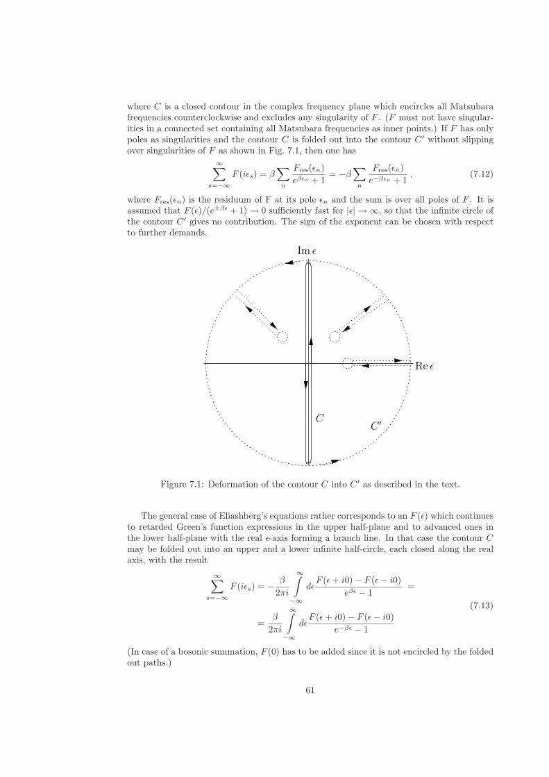
where C is a closed contour in the complex frequency plane which encircles all Matsubarafrequencies counterclockwise and excludes any singularity of F . (F must not have singular-ities in a connected set containing all Matsubara frequencies as inner points.) If F has onlypoles as singularities and the contour C is folded out into the contour C ′ without slippingover singularities of F as shown in Fig. 7.1, then one has

∞∑

s=−∞

F (iǫs) = β∑

n

Fres(ǫn)

eβǫn + 1= −β

∑

n

Fres(ǫn)

e−βǫn + 1, (7.12)

where Fres(ǫn) is the residuum of F at its pole ǫn and the sum is over all poles of F . It isassumed that F (ǫ)/(e±βǫ + 1) → 0 sufficiently fast for |ǫ| → ∞, so that the infinite circle ofthe contour C ′ gives no contribution. The sign of the exponent can be chosen with respectto further demands.

Im ǫ

Re ǫ

CC

′

Figure 7.1: Deformation of the contour C into C ′ as described in the text.

The general case of Eliashberg’s equations rather corresponds to an F (ǫ) which continuesto retarded Green’s function expressions in the upper half-plane and to advanced ones inthe lower half-plane with the real ǫ-axis forming a branch line. In that case the contour Cmay be folded out into an upper and a lower infinite half-circle, each closed along the realaxis, with the result

∞∑

s=−∞

F (iǫs) = − β

2πi

∞∫

−∞

dǫF (ǫ+ i0) − F (ǫ− i0)

eβǫ − 1=

=β

2πi

∞∫

−∞

dǫF (ǫ+ i0) − F (ǫ− i0)

e−βǫ − 1

(7.13)

(In case of a bosonic summation, F (0) has to be added since it is not encircled by the foldedout paths.)

61

When applied to (7.5–7.8), one must realize that λ(ω) inherits the branch line of thephonon Green’s functionD(ω) as readily seen from (5.31). Hence one has to insert (5.31) and(5.33) into Eliashberg’s equations before one can make these transformations. In the dirtylimit, (5.34) may be inserted instead. As regards the continuation of the Green’s function(7.3, 7.4) to the real frequency axis, one first uses a notation iǫs(κ) = iǫ(κ; iǫs) = iǫsZ(κ; iǫs)which implies iǫ(κ; ǫ) = ǫZ(κ; ǫ) by replacing iǫs with ǫ. With the same replacements oneobtains

g(κ; ǫ) = −π ǫZ(κ; ǫ)√

−ǫ2Z2(κ; ǫ) + |φ(κ; ǫ)|2, f(κ; ǫ) = π

φ(κ; ǫ)√

−ǫ2Z2(κ; ǫ) + |φ(κ; ǫ)|2(7.14)

with branch lines of the square root on the real ǫ-axis for |ǫZ(κ; ǫ)| > |φ(κ; ǫ)|. This makesconnection to the real frequency representations of Eliashberg’s equations in the literaturewhich are usually given in the dirty limit, that is, averaged over κ.

7.2 The Quasiparticle Density of States

As seen from the definition (3.6), the Nambu component G11 of the Green’s function isthe normal electron propagator. Its analytic continuation from the positive imaginary Mat-subara frequencies to the real frequency axis yields the retarded propagator which, if itcontinues to a pole on the ‘unphysical sheet’ of the Riemannian surface of Gr below the realaxis, describes a quasi-particle excitation according to (2.18–2.20).

Strictly speaking, the analytic properties can only be taken for granted for the fullGreen’s functions G = Glow + Ghigh. If this splitting were made in an analytic way, nopart would be exactly zero in any frequency region because as an analytic function it thenwould automatically be zero for all frequencies. At best one can expect that Glow is a verygood approximation to the full G for low values |ǫ|, and governs the analytic continuationof the full Gr in the region of interest. (Anyhow, the analytic continuation to a pole in(2.18–2.20) was a mere vehicle to describe Lorentzian shape features of ImGr on the realǫ-axis.) The same considerations with negative Matsubara frequencies apply to Ga. In thisunderstanding we consider the analytic continuation of the right expression of (7.1) to the

real frequency axis to be a good approximation to Gr/a11 . We change the energy notation in

this expression to ǫκ in order not to confuse it with the general complex frequency ǫ, andintroduce again a notation

iǫ(κ; ǫ) = ǫZ(κ; ǫ) (7.15)

for generally complex frequencies ǫ. Recalling that λ(κ,κ′; iωs) or λ(iωs) depends on ω2s

only (cf. (5.33, 5.34)), it can be inferred from (7.5) or (7.7) that ǫs(κ) = −ǫ−s(κ). Moreover,(7.15) is purely imaginary for imaginary ǫ in the frame of our approximations (since λ isreal). Hence, Z(κ; ǫ) is a real and even function of imaginary ǫ. If it is analytic aroundǫ = 0, then its Taylor expansion has only even orders with real coefficients, which meansthat Z is also a real and even function of real ǫ. We introduce additionally the notation

|φ(κ; ǫ)|2 = ∆2(κ; ǫ)Z2(κ; ǫ), (7.16)

where consequently ∆ must also be real. Then, for ǫ real and low, the right expression of(7.1) yields

gr11(κǫκ; ǫ) =

ǫZ(κ; ǫ) + ǫκǫ2Z2(κ; ǫ) − ǫ2κ − ∆2(κ; ǫ)Z2(κ; ǫ)

≈

≈ A+(κ, ǫκ)

ǫ−√

ǫ2κ/Z2(κ) + ∆2(κ)

+A−(κ, ǫκ)

ǫ+√

ǫ2κ/Z2(κ) + ∆2(κ)

,

(7.17)

62

where we further approximated Z(κ; ǫ) ≈ Z(κ; 0) = Z(κ), ∆(κ; ǫ) ≈ ∆(κ; 0) = ∆(κ). Thespectral weights are

A±(κ, ǫκ) =1

2Z(κ)

(

1 ∓ ǫκ/Z(κ)√

ǫ2κ/Z2(κ) + ∆2(κ)

)

. (7.18)

From these expressions one reads off the quasi-particle energies

E(κ, ǫκ) ≈√

ǫ2κ/Z2(κ) + ∆2(κ) (7.19)

with an excitation gap ∆(κ).At each point κ of the Fermi surface, the bandstructure energies ±ǫκ both contribute to

both quasi-particle poles (7.17) (of electron and hole type), and their common contributionin both cases is

A±(κ, ǫκ) +A±(κ,−ǫκ) = Z−1(κ). (7.20)

The total quasi-particle spectral density is obtained as

D(ǫ) ≈∫

d2κd(κ)

∫

dǫκ Z−1(κ)δ(ǫ− E(κ, ǫκ)). (7.21)

Note that these last considerations are only semi-quantitatively correct. A more accurateapproach needs a numerical analysis of the first line of (7.17).

7.3 The Thermodynamic Critical Field

To calculate the Inner Energy of the system we return to (2.66) and transform it with thehelp of (2.32) into

〈W 〉 =iζ

2lim

τ→−0

∫

dxdx1

(

δ(x− x1)∂

∂τ+ h0(x, x1)

)

i

β

∑

s

e−iǫsτG(x1, x; iǫs) =

=ζ

2βlimτ→0

∑

s

eiǫsτ

∫

dxdx1

(

∑

kn

φkn(x)φ∗kn(x1)iǫs−

−∑

kn,k′n′

∫

dx′dx′1φkn(x)φ∗kn(x′)h0(x′, x′1)φk′n′(x′1)φ∗k′n′(x1)

)

G(x1, x; iǫs) =

=ζ

2βlimτ→0

∑

s

eiǫsτ∑

kn

(

iǫs − ǫkn

)

G(k, n, n; iǫs).

(7.22)

In the second equality we replaced the δ-function by a completeness relation of Bloch eigen-functions of h0 and inserted in the same manner two further integrals over δ-functions.

With (2.64), the expectation value of h0 is

〈h0〉 =

∫

dxdx1 h0(x, x1)n1(x1|x) = −iζ lim

τ→−0

∫

dxdx1 h0(x, x1)G(x1, x;−iτ) =

=ζ

βlimτ→0

∑

s

eiǫsτ∑

kn

ǫknG(k, n, n; iǫs).(7.23)

These two results may be combined to yield the Inner Energy E = 〈h0 + W 〉 as

E =ζ

2βlimτ→0

∑

s

eiǫsτ∑

kn

(

iǫs + ǫkn)G(k, n, n; iǫs). (7.24)

63

The eigenvalues ǫkn of the grand canonical Hamiltonian h0 (band structure) are again mea-sured from the chemical potential µ.

Although it was not considered in Section 2.8, it is clear from the derivation given therethat 〈W 〉 contains all interaction energies of electrons with other particles appearing in theHamiltonian in interaction terms with the electrons, notably phonons. It does not containthe single-particle energies of those other particles which would have to be added in analogyto (7.23).

For the undressed phonons one has

D(q, λ, λ;−iτ) = − i

M

∑

ll′

e−iq·(Rl−R′

l)⟨

Tτ

[

ulλ(−iτ)ul′λ(0)]

⟩

=

= − i

2ΩqλMqλ

(⟨

Tτ

[

bqλ(−iτ)b†qλ(0)]

⟩

+⟨

Tτ

[

b†qλ(−iτ)bqλ(0)]

⟩

.

(7.25)

Hence,2iΩqλMqλD(q, λ, λ; τ = 0) =

⟨

bqλb†qλ

⟩

+⟨

b†qλbqλ

⟩

= 2nqλ + 1, (7.26)

and

〈hph〉 =∑

qλ

Ωqλ

(

nqλ +1

2

)

=−1

β

∑

s

∑

qλ

MqλΩ2qλD(q, λ, λ; iωs), (7.27)

which has a structure analogous to (7.23). We used a notation of ‘mode masses’ in the spiritof (4.13), that is Mqλ =

∑

κ eλ(qκ)e∗λ(qκ) with properly normalized polarization vectors asin (4.13). The Ωqλ are the frequencies of the bare ionic lattice without electrons (but ofcourse with a neutralizing charged homogeneous background).

The thermodynamic critical field Bc of the superconducting state is defined as

V B2c

2µ0= EN − ES = ∆E, (7.28)

where ES is the Inner Energy of the superconducting state and EN is the normal statereference energy of a thermodynamic state in which the anomalous self-energy φs(κ) isforced to be zero. (It can likewise be defined with the Free Energy difference, since smallchanges are the same in all thermodynamic potentials.) If we use the same indexing for theGreen’s functions, we have

V B2c

2µ0=

1

2β

∑

s

(

∑

kn

(iǫs + ǫkn)(

GN(k, n, n; iǫs) −GS(k, n, n; iǫs))

−

− 2∑

qλ

MqλΩ2qλ

(

DN(q, λ, λ; iωs) −DS(q, λ, λ; iωs))

)

.

(7.29)

Since the difference between the normal and superconducting Green’s functions vanishesrapidly with increasing frequencies, we need not bother any more about the τ -limes. Ofcourse, GS is again the Nambu 11-component of the Green’s function.

The electronic quasi-particle renormalization of Section 5.1 is not specific for the su-perconducting state. The electronic Green’s functions in (7.29) may be replaced by therenormalized ones, gN and gS. The band structure ǫkn is then of course also to be takenrenormalized, that is, with the potential (5.12).

Although the modification of the phonon Green’s function D from the normal to su-perconducting state does to leading order not influence the electron self-energy, it can notbe neglected in (7.29). Nevertheless, the phonons in both states may be considered inharmonic approximation, whence (7.27) is just twice the kinetic energy T of the nuclei.

64

The kinetic energy T is homogeneous linear in the inverse average of the nuclear masses,µ = 〈1/Mλ〉: µ(∂/∂µ)T = T . If the superconductor condensation energy (7.28) has anisotopic dependence µ2α (that is, Hc ∼ µα), then, by a Hellmann-Feynman argument,2α∆E = µ(∂/∂µ)∆E = µ∆

⟨

(∂/∂µ)H⟩

= ∆T. Hence, the second line of (7.29), which is2∆T , is 4α times the left hand side. If we additionally insert (7.17) and its normal statecounterpart (with ∆(κ, ǫ) = 0) into the first line, we obtain a semi-phenomenological expres-sion (depending on the phenomenological isotope exponent α) for the condensation energyand hence for the thermodynamic critical field:

V B2c

2µ0=

1

4α− 1

1

2β

∑

s

∑

kn

(iǫs + ǫkn) ·

·(

iǫsZS(κ, iǫs) + ǫkn

ǫ2sZ2S(κ, iǫs) + ǫ2kn + ∆2(κ, iǫs)Z2

S(κ, iǫs)+

1

iǫsZN(κ, iǫs) − ǫkn

)

.

(7.30)

Again, by means of the summation technique described in Section 7.1, there are differentways of writing these results possible which are met in the literature. By moving between thereal and imaginary frequency axis for the various parts of the expressions to be calculatedone may optimize the numerical effort and stabilize the numerical convergence of the routinesused. These are, however, technical problems, although of practical importance.

65