ORIGINAL PAPER

Microscale mechanical modeling of deformable geomaterialswith dynamic contacts based on the numerical manifold method

Mengsu Hu1& Jonny Rutqvist1

Received: 2 May 2020 /Accepted: 24 July 2020# The Author(s) 2020

AbstractMicromechanical modeling of geomaterials is challenging because of the complex geometry of discontinuities and potentiallylarge number of deformable material bodies that contact each other dynamically. In this study, we have developed a numericalapproach for micromechanical analysis of deformable geomaterials with dynamic contacts. In our approach, we detect contactsamong multiple blocks with arbitrary shapes, enforce different contact constraints for three different contact states of separated,bonded, and sliding, and iterate within each time step to ensure convergence of contact states. With these features, we are able tosimulate the dynamic contact evolution at the microscale for realistic geomaterials having arbitrary shapes of grains and inter-faces. We demonstrate the capability with several examples, including a rough fracture with different geometric surface asperitycharacteristics, settling of clay aggregates, compaction of a loosely packed sand, and failure of an intact marble sample. With ourmodel, we are able to accurately analyze (1) large displacements and/or deformation, (2) the process of high stress accumulated atcontact areas, (3) the failure of a mineral cemented rock samples under high stress, and (4) post-failure fragmentation. Theanalysis highlights the importance of accurately capturing (1) the sequential evolution of geomaterials responding to stress asmotion, deformation, and high stress; (2) large geometric features outside the norms (such as large asperities and sharp corners) assuch features can dominate the micromechanical behavior; and (3) different mechanical behavior between loosely packed andtightly packed granular systems.

Keywords Dynamic contacts . Bonded and sliding . Cohesion and tensile strength . Fracture asperities . Granular systems .

Numerical manifoldmethod

1 Introduction

Numerical modeling of microscale mechanical behavior ofgeomaterials (soils and rocks) is of great importance for un-derstanding and predicting material constitutive andgeomechanical behavior at larger scales in subsurface engi-neering activities such as unconventional hydrocarbon pro-duction [22], nuclear waste disposal [23], and CO2 sequestra-tion [21]. Some unique features of geomaterials are that theyare naturally stressed and heated to variable degrees, and often

fluid filled. The microscale structure of geomaterials containsminerals, pores, and fractures of complex shapes that evolveas a result of coupled fluid, heat, mechanics, and chemicalreactions. In order to understand such dynamic multiphysicsproblems, in the past decade, new technologies have beendeveloped for visualization and characterization of themultiphysics processes of geomaterials at the pore scale, mi-croscale, and even smaller scales [16, 20, 31, 33, 38].

However, numerical modeling of mechanical processes ingeomaterials at the microscale is challenging because of thecomputational geometry associated with (1) complex evolv-ing geometric features that are discontinuous, and (2) multipledeformable material bodies with dynamic contacts. At themicroscale, geomaterials exhibit more complex geometric fea-tures that cannot be simplified easily and therefore lead todiscontinuities in physical fields (i.e., displacements and stressfor mechanics). Moreover, in addition to the force balance,microscale mechanical processes may involve large deforma-tion, large translational or rotational displacements, and

* Mengsu Humengsuhu@lbl.gov

Jonny Rutqvistjrutqvist@lbl.gov

1 Energy Geosciences Division, Lawrence Berkeley NationalLaboratory, Berkeley, CA 94720, USA

https://doi.org/10.1007/s10596-020-09992-z

/ Published online: 5 August 2020

Computational Geosciences (2020) 24:1783–1797

dynamic contacts. The grand challenge of computing contactsis to identify when and where contacts occur among manyblocks [27]. This is complicated by the fact that these blocksare moving, deforming, and in some cases breaking apart. Inturn, motion, deformation, and breakage of blocks are impact-ed by contact forces, thus constituting a serial process.Inaccurate calculation of contacts, therefore, can lead tocompletely erroneous overall system behavior.

For systems involving both continua and discontinua suchas single fractures at the asperity scale, various models havebeen developed to simulate fluid flow [1, 39], heat transfer[18], reactive transport [28], or their couplings [3]. But numer-ical models that fully address contacts and deformation incombination are much rarer due to the aforementioned chal-lenges. For computation of granular materials, a number ofnumerical approaches based on the discrete element method(DEM) have been developed, including those of Cundall [5],Houlsby [8] and Andrade et al. [2]. Though DEM is designedfor computation of discontinuous bodies with dynamic con-tacts, the assumption of rigid bodies, the use of explicit timeiteration, and the limitation of interpolation fields for contin-uum mechanics limit its accuracy for dealing with realisticgeometric features or dynamic contacts. These limitationsare in addition to its potentially high computational cost. Onthe other hand, a number of approaches have been developedusing the finite element method (FEM) to enable contact cal-culations (Puso and Laursen, [40]; [24]). Though FEM ispowerful for continuum mechanics possibly involving largedeformation, the common contacting algorithms developed inthose approaches assume that contacts are along prefixed con-tact pairs, or generally do not involve multi-body system or alarge number of contacting pairs. Some other approaches havebeen developed for contacts in granular systems, but these donot overcome the fundamental limitations associated withprefixed contact pairs, a limited number of contacts, or thelimited accuracy for either continuum or discontinuum calcu-lations. Therefore, there is a need to develop a powerfultoolset that can accurate capture both continuous and discon-tinuous behavior involving dynamic contacts that may involvea large number of interacting material bodies.

The numerical manifold method (NMM, [25, 26]) is apromising method for analyzing both continuous and discon-tinuous media involving dynamic contacts. NMM is based onthe theory of mathematical manifolds. The numerical meshesof NMM consist of mathematical covers and physical covers.The mathematical covers overlay the entire material domainand the physical covers are divided from the mathematicalcovers by boundaries and discontinuities. Based on thisdual-mesh concept, both continuous and discontinuous prob-lems can be rigorously solved by flexibly defining physicalcovers. In the past two decades, NMM has been successfullyapplied to mechanics analysis of both continuous and discon-tinuous geologic media [17], involving higher-order

interpolation [4], fracture propagation [36], wave propagationthrough fractured media [6], analysis of slope stability [7, 19],and microscale-macroscale modeling of fracturing of sand-stone [34]. Most recently, the authors developed a numberof models for analyzing flow and fully coupled hydro-mechanical processes of fractured porous media at differentscales ([13–15], [9]).

In this paper, we present development of an approach withrigorous treatment of dynamic contacts in deformable geoma-terials for microscale mechanical analysis based on the NMM.We first present a general mathematical description of theproblem of deformable geomaterial bodies with dynamic con-tacts in Section 2. Then, we introduce the approach of model-ing continuum and discontinuum mechanics based on theNMM, including the fundamentals for global continuousand discontinuous interpolation, and a rigorous multi-step ap-proach for contact calculations in Section 3. In Section 4, weapply this approach to a number of examples at the micro-scale, including a single fracture at the asperity scale, granularsystems of aggregated clay settling, compaction of a looselypacked sand, and failure of a cemented marble sample. InSection 5, we conclude and provide perspectives for futuredirections.

2 Mathematical statement of deformablegeomaterial bodies with dynamic contacts

A single continuum or discontinuum material body in dynam-ic states satisfies force balance:

∇ � σþ f¼ρ∂2u∂t2

ð1Þ

where σ is the stress tensor, f is the body force vector, ρ is thedensity of the material body, u is the vector of displacements,and t is time. At steady state, the right-hand side representingthe inertia terms = 0.

The force term is not only a result of loading (Fl), but isalso present whenmaterial bodies are discontinuous and are incontact (i.e., the contact force, Fcontact). Thus, the completeexpression of the force includes both terms as follows:

F ¼ Fl þ Fcontact ð2Þ

In order to include continuum and discontinuummechanicsin a unified way, we express the displacement as:

u ¼ ∫εdsþ utr þ ur ð3Þwhere the displacement includes not only the term that is dueto deformation ∫εds, but also the translational utr and rotation-al ur displacements. When the deformation is assumed small,strain is known as the spatial derivative of displacements.

1784 Comput Geosci (2020) 24:1783–1797

With introduction of translational and rotational displace-ments, the motion of a material body can be described.

When a material body does not interact with other materialbodies, in response to loading, it may move or deform beforethe stress reaches the strength of the material. Various types ofcontinuum constitutive laws with different stress-strain rela-tionships have been developed to describe the continu-um behavior of a material body, which can beexpressed generally as:

σ ¼ g εð Þ ð4Þwhere g is a general function, which can be linear,nonlinear, or rate-dependent. For example, Hooke’slaw is most widely used law to describe the linear elas-tic relationship between the stress and strain tensors.

When a material body interacts with other material bodies,conventional continuum constitutive laws are not sufficient todescribe the relationships between contact forces and dis-placements and/or deformations associated with contacts.Between different material bodies, it is more natural to usethe distance d and the relative displacement in the directionalong the contacting face ⟦us⟧ to describe their state of con-tacts. Here the distance d is the distance between a contact pair(i.e., the exact contacting vertices and/or surfaces between twomaterial bodies). The distance d includes time-dependent in-fluences of relative displacement and relative deformation ofthe twomaterial bodies between the potential contacting faces.Thus, a general expression of contact force as a function of dand ⟦us⟧ can be expressed as:

Fcontact ¼ h d;〚us〛ð Þ ð5Þwhere ⟦us⟧ denotes discontinuity of displacements (i.e., rela-tive displacements) between a contact pair in the directionalong the contacting face, and h is a function of d and ⟦us⟧,both of which may be dynamically changing before reachingequilibrium.

With or without considering motion or deformation of ma-terial bodies, there are always three possible relative positionsbetween two material bodies A and B: (1) A and B are sepa-rated (no contact anywhere); (2) A and B are bonded to eachother on the vertices or surfaces of the body; and (3) A ismoving along B while A is in contact with B, and such amotion is sliding. For these three different contact states, theirrespective functions h are different.

When A and B are separated, in most cases there are nocontact forces between them. Thus, we have:

h ¼ 0 ð6Þ

In rare cases, for example when there is an electrical doublelayer, there are forces between A and B, but this effect is notcurrently included in this study.

When A and B are bonded, the distance between A and Bon the contacting pair (vertices and/or edges in 2D) should bezero, and the relative displacement along the contacting face⟦us⟧ should be zero as well, satisfying:

d ¼ 0 ∩〚us〛¼ 0 ð7Þ

Note that in Eq. (7), we still consider the situations when Aand B are moving and deforming, but remaining bonded toeach other.

When A is sliding along B while A is in contact with B, thecontact occurs at the sliding face. On this face, there is nodistance between A and B, while the sliding satisfies certainfriction laws. We use the Coulomb’s law of friction to de-scribe sliding along the contact face for the sliding state:

d ¼ 0 ∩ Fs ¼ F0ntanφsgn〚us〛ð Þ ð8Þ

where Fs denotes the contacting force in the direction of the

sliding face, F0n denotes the effective contact force in the

direction normal to the contact face (here effective meanseliminating force associated with water pressure), φ is thefriction angle, and sgn(⟦us⟧) means the direction of Fs thatdepends on the direction of relative shear displacement.

Although in Eqs. (7)–(8) there is no explicit description ofthe contact forces, the distance and/or relative displacementconstraints function like implicit boundary conditions. Theseconstraints on the contact faces can be imposed with differentapproaches, such as with a penalty method [25], Lagrangemultiplier method [11], and the most advanced approachbased on the variational inequality method [37], leading toforce terms as contact forces. Numerical implementation ofthese boundary constraints will be introduced in more detailin the next section.

So far, we have described two individual material bodies inseparated, bonded, and sliding contact states. In dynamic con-ditions, these contact states may be changed as follows:

If material bodies A and B were not in contact (separat-ed), but become bonded later, constraints in Eq. (7)should be added. If A and B were not in contact, but thenthey are in sliding state, constraints in Eq. (8) should beadded.If material bodies A and B were bonded but becomeseparated later, we need to consider one condition: Inorder to separate A from B, the effective force in the

direction normal to the contacting face F0n needs to be

larger than the force associated with the tensile strengthT. That is because in a rather long geological period as aresult of thermal-hydro-mechanical-chemical(THMC) processes, adhesion and/or tensile bondstrength can be gained between A and B along theircontacting faces. This criterion for separating two

1785Comput Geosci (2020) 24:1783–1797

bonded bodies in the direction normal to their con-tact face can be expressed as:

F0n > T ð9Þ

If Eq. (9) is satisfied, the two material bodies are no lon-ger in contact; therefore, the constraints in Eq. (8) shouldbe removed.If material bodies A and B were bonded but transfer to asliding state, we need to consider one condition: In orderto initiate sliding of A and B against each other, the forcein the direction of contacting face Fs needs to be largerthan the shear strength S. The shear strength could begained as a result of THMC processes, consisting of fric-tional force (satisfying Coulomb’s law of friction) andcohesive force Fcohe. This criterion for shearing twobonded bodies in the direction along their contact facecan be expressed as:

Fs > S ¼ F0ntanφ

0 þ Fcohe ð10Þwhere φ′ is the internal friction angle. If Eq. (10) is satis-fied, the two material bodies are transferred from bondedto sliding state. Comparing Eq. (7) and (8), we find thatthe constraint in the direction normal to contacting faceshould be retained, while in the sliding direction, the con-straint needs to be changed.If A and B slide on each other but become separated,constraints in Eq. (9) should be removed. If they becomebonded, the constraints should be modified in the direc-tion of the contacting face so that no relative shear dis-placement will occur.With Eqs. (6)–(10), we are able to describe the threedifferent contact states of two material bodies, dynamicchanges of these contact states, and criteria that need to besatisfied for changes of the contact states.

3 Modeling continuum-discontinuummechanics with NMM

3.1 Fundamentals of NMM: global approximation

The numeral manifold method (NMM) [25] is based on theconcept of a “manifold” in topology. In NMM, independentmeshes for interpolation and integration are defined separately.Based on this unique definition, a non-conforming mesh (notnecessarily conforming with the physical boundaries) can beused as a mathematical mesh. Different local approximationfunctions can be constructed and averaged to establish globalapproximations for both continuous and discontinuous analysis.

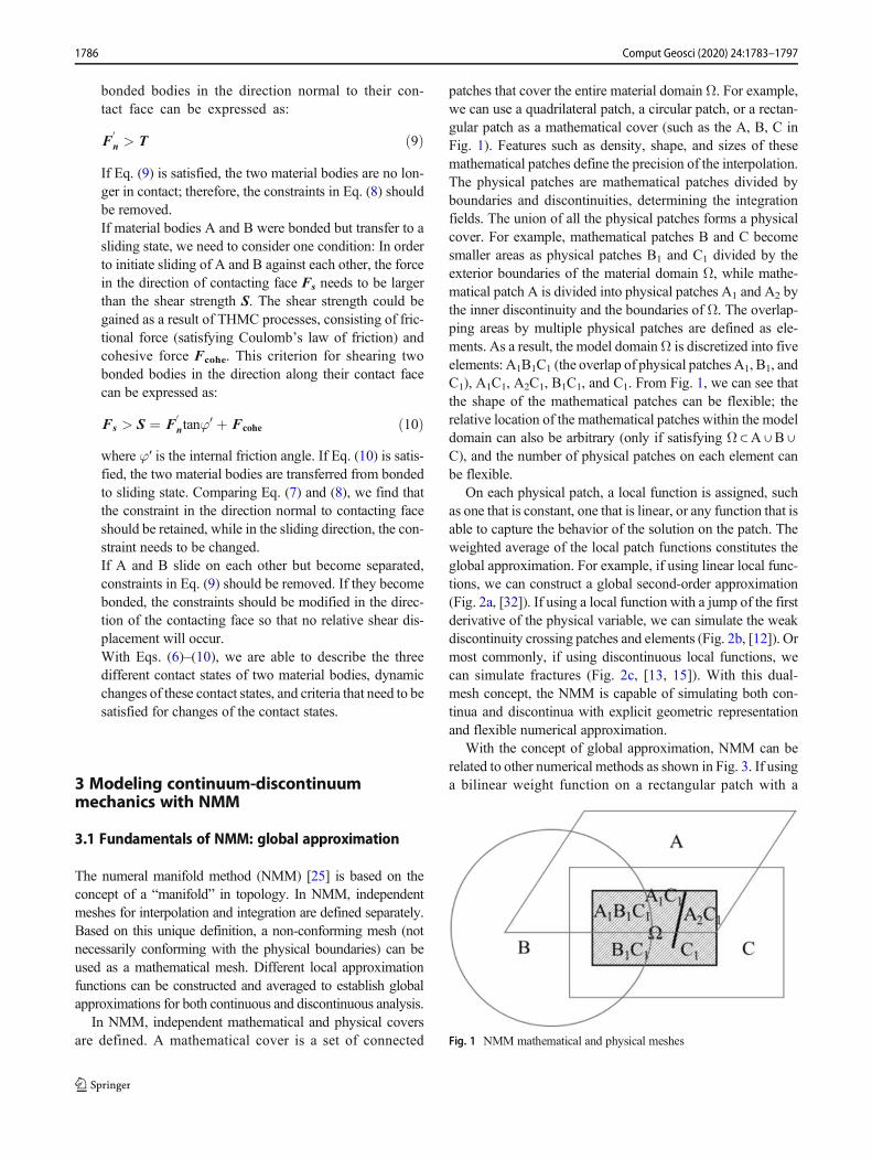
In NMM, independent mathematical and physical coversare defined. A mathematical cover is a set of connected

patches that cover the entire material domain Ω. For example,we can use a quadrilateral patch, a circular patch, or a rectan-gular patch as a mathematical cover (such as the A, B, C inFig. 1). Features such as density, shape, and sizes of thesemathematical patches define the precision of the interpolation.The physical patches are mathematical patches divided byboundaries and discontinuities, determining the integrationfields. The union of all the physical patches forms a physicalcover. For example, mathematical patches B and C becomesmaller areas as physical patches B1 and C1 divided by theexterior boundaries of the material domain Ω, while mathe-matical patch A is divided into physical patches A1 and A2 bythe inner discontinuity and the boundaries of Ω. The overlap-ping areas by multiple physical patches are defined as ele-ments. As a result, the model domainΩ is discretized into fiveelements: A1B1C1 (the overlap of physical patches A1, B1, andC1), A1C1, A2C1, B1C1, and C1. From Fig. 1, we can see thatthe shape of the mathematical patches can be flexible; therelative location of the mathematical patches within the modeldomain can also be arbitrary (only if satisfying Ω ⊂A ⋃B ⋃C), and the number of physical patches on each element canbe flexible.

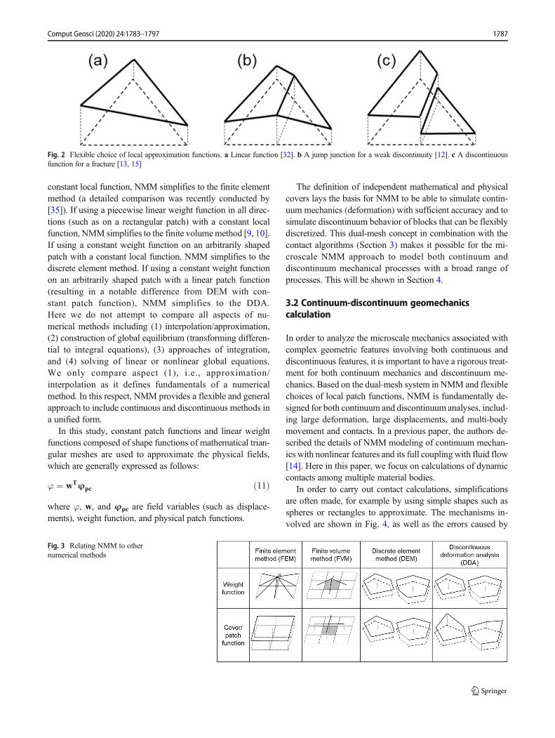
On each physical patch, a local function is assigned, suchas one that is constant, one that is linear, or any function that isable to capture the behavior of the solution on the patch. Theweighted average of the local patch functions constitutes theglobal approximation. For example, if using linear local func-tions, we can construct a global second-order approximation(Fig. 2a, [32]). If using a local function with a jump of the firstderivative of the physical variable, we can simulate the weakdiscontinuity crossing patches and elements (Fig. 2b, [12]). Ormost commonly, if using discontinuous local functions, wecan simulate fractures (Fig. 2c, [13, 15]). With this dual-mesh concept, the NMM is capable of simulating both con-tinua and discontinua with explicit geometric representationand flexible numerical approximation.

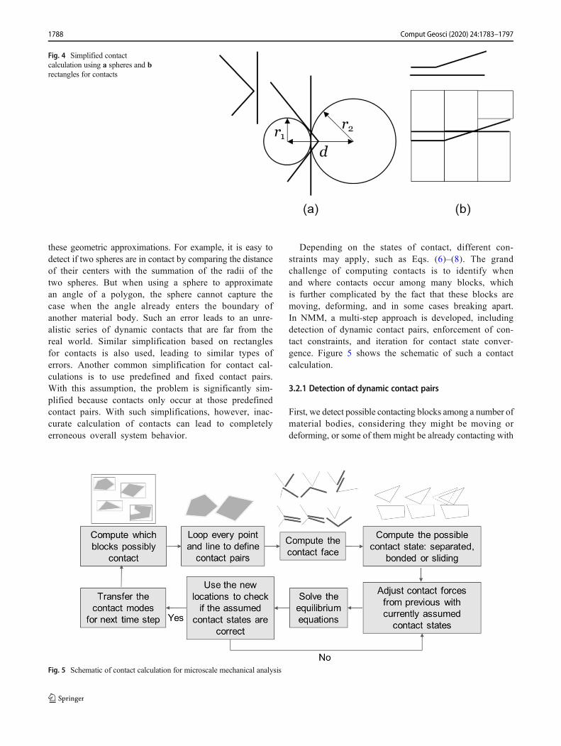
With the concept of global approximation, NMM can berelated to other numerical methods as shown in Fig. 3. If usinga bilinear weight function on a rectangular patch with a

Fig. 1 NMM mathematical and physical meshes

1786 Comput Geosci (2020) 24:1783–1797

constant local function, NMM simplifies to the finite elementmethod (a detailed comparison was recently conducted by[35]). If using a piecewise linear weight function in all direc-tions (such as on a rectangular patch) with a constant localfunction, NMM simplifies to the finite volumemethod [9, 10].If using a constant weight function on an arbitrarily shapedpatch with a constant local function, NMM simplifies to thediscrete element method. If using a constant weight functionon an arbitrarily shaped patch with a linear patch function(resulting in a notable difference from DEM with con-stant patch function), NMM simplifies to the DDA.Here we do not attempt to compare all aspects of nu-merical methods including (1) interpolation/approximation,(2) construction of global equilibrium (transforming differen-tial to integral equations), (3) approaches of integration,and (4) solving of linear or nonlinear global equations.We only compare aspect (1), i.e., approximation/interpolation as it defines fundamentals of a numericalmethod. In this respect, NMM provides a flexible and generalapproach to include continuous and discontinuous methods ina unified form.

In this study, constant patch functions and linear weightfunctions composed of shape functions of mathematical trian-gular meshes are used to approximate the physical fields,which are generally expressed as follows:

φ ¼ wTφpc ð11Þ

where φ, w, and φpc are field variables (such as displace-ments), weight function, and physical patch functions.

The definition of independent mathematical and physicalcovers lays the basis for NMM to be able to simulate contin-uum mechanics (deformation) with sufficient accuracy and tosimulate discontinuum behavior of blocks that can be flexiblydiscretized. This dual-mesh concept in combination with thecontact algorithms (Section 3) makes it possible for the mi-croscale NMM approach to model both continuum anddiscontinuum mechanical processes with a broad range ofprocesses. This will be shown in Section 4.

3.2 Continuum-discontinuum geomechanicscalculation

In order to analyze the microscale mechanics associated withcomplex geometric features involving both continuous anddiscontinuous features, it is important to have a rigorous treat-ment for both continuum mechanics and discontinuum me-chanics. Based on the dual-mesh system in NMM and flexiblechoices of local patch functions, NMM is fundamentally de-signed for both continuum and discontinuum analyses, includ-ing large deformation, large displacements, and multi-bodymovement and contacts. In a previous paper, the authors de-scribed the details of NMM modeling of continuum mechan-ics with nonlinear features and its full coupling with fluid flow[14]. Here in this paper, we focus on calculations of dynamiccontacts among multiple material bodies.

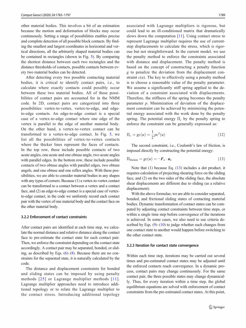
In order to carry out contact calculations, simplificationsare often made, for example by using simple shapes such asspheres or rectangles to approximate. The mechanisms in-volved are shown in Fig. 4, as well as the errors caused by

Fig. 3 Relating NMM to othernumerical methods

Fig. 2 Flexible choice of local approximation functions. a Linear function [32]. b A jump junction for a weak discontinuity [12]. c A discontinuousfunction for a fracture [13, 15]

1787Comput Geosci (2020) 24:1783–1797

these geometric approximations. For example, it is easy todetect if two spheres are in contact by comparing the distanceof their centers with the summation of the radii of thetwo spheres. But when using a sphere to approximatean angle of a polygon, the sphere cannot capture thecase when the angle already enters the boundary ofanother material body. Such an error leads to an unre-alistic series of dynamic contacts that are far from thereal world. Similar simplification based on rectanglesfor contacts is also used, leading to similar types oferrors. Another common simplification for contact cal-culations is to use predefined and fixed contact pairs.With this assumption, the problem is significantly sim-plified because contacts only occur at those predefinedcontact pairs. With such simplifications, however, inac-curate calculation of contacts can lead to completelyerroneous overall system behavior.

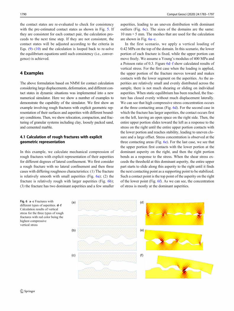
Depending on the states of contact, different con-straints may apply, such as Eqs. (6)–(8). The grandchallenge of computing contacts is to identify whenand where contacts occur among many blocks, whichis further complicated by the fact that these blocks aremoving, deforming, and in some cases breaking apart.In NMM, a multi-step approach is developed, includingdetection of dynamic contact pairs, enforcement of con-tact constraints, and iteration for contact state conver-gence. Figure 5 shows the schematic of such a contactcalculation.

3.2.1 Detection of dynamic contact pairs

First, we detect possible contacting blocks among a number ofmaterial bodies, considering they might be moving ordeforming, or some of them might be already contacting with

Fig. 4 Simplified contactcalculation using a spheres and brectangles for contacts

Fig. 5 Schematic of contact calculation for microscale mechanical analysis

1788 Comput Geosci (2020) 24:1783–1797

other material bodies. This involves a bit of an estimationbecause the motion and deformation of blocks may occurcontinuously. Setting a range of possibilities enables preciseand complete detection of all possible block contacts. By find-ing the smallest and largest coordinates in horizontal and ver-tical directions, all the arbitrarily shaped material bodies canbe contained in rectangles (shown in Fig. 5). By comparingthe shortest distance between each two rectangles and thedistance thresholds of contacts, possible contacts between ev-ery two material bodies can be detected.

After detecting every two possible contacting materialbodies, it is critical to identify contact pairs, i.e., tocalculate where exactly contacts could possibly occurbetween these two material bodies. All of these possi-bilities of contact pairs are accounted for in the NMMcode. In 2D, contact pairs are categorized into threepossibilities: vertex-to-vertex, vertex-to-edge, and edge-to-edge contacts. An edge-to-edge contact is a specialcase of a vertex-to-edge contact where one edge of thevertex is parallel to the edge of another material body.On the other hand, a vertex-to-vertex contact can betransformed to a vertex-to-edge contact. In Fig. 5, welist all the possibilities of vertex-to-vertex contactswhere the thicker lines represent the faces of contacts.In the top row, these include possible contacts of twoacute angles, one acute and one obtuse angle, two acute angleswith parallel edges. In the bottom row, these include possiblecontacts of two obtuse angles with parallel edges, two obtuseangels, and one obtuse and one reflex angles. With these pos-sibilities, we are able to consider material bodies in any shapeswith any types of corners. Because (1) a vertex-to-vertex contactcan be transformed to a contact between a vertex and a contactface, and (2) an edge-to-edge contact is a special case of vertex-to-edge contact, in the code we uniformly record each contactpair with the vertex of onematerial body and the contact face onthe other material body.

3.2.2 Enforcement of contact constraints

After contact pairs are identified at each time step, we calcu-late the normal distance and relative distance along the contactface to pre-estimate the contact state for each contact pair.Then, we enforce the constraint depending on the contact stateaccordingly. A contact pair may be separated, bonded, or slid-ing, as described by Eqs. (6)–(8). Because there are no con-straints for the separated state, it is naturally calculated by thecode.

The distance and displacement constraints for bondedand sliding states can be imposed by using penaltymethods [25] or Lagrange multiplier methods [11].Lagrange multiplier approaches need to introduce addi-tional topology or to relate the Lagrange multiplier tothe contact stress. Introducing additional topology

associated with Lagrange multipliers is rigorous, butcould lead to an ill-conditioned matrix that dramaticallyslows down the computation [11]. Using contact stress torepresent Lagrange multiplier requires the use of current-step displacements to calculate the stress, which is rigor-ous but not straightforward. In the current model, we usethe penalty method to enforce the constraints associatedwith distance and displacement. The penalty method isbased on the concept of constructing a penalty functiong to penalize the deviation from the displacement con-straint c(u). The key to effectively using a penalty methodis to choose a reasonable value of the penalty parameter.We assume a significantly stiff spring applied to the de-viation of a constraint associated with displacements.Therefore, the stiffness of the spring becomes the penaltyparameter p. Minimization of deviation of the displace-ment constraint can be achieved by minimizing the poten-tial energy associated with the work done by the penaltyspring. The potential energy Πc by the penalty spring toenforce the constraint can be generally expressed as:

Πc ¼ gc uð Þ ¼ 1

2pc2 uð Þ ð12Þ

The second constraint, i.e., Coulomb’s law of friction, isimposed directly by constructing the potential energy:

Πfriction ¼ gc uð Þ ¼ −Fs � us ð13Þ

Note that (1) because Eq. (13) includes a dot product, itrequires calculation of projecting shearing force on the slidingface, and (2) on the two sides of the sliding face, the absoluteshear displacements are different due to sliding (as a relativedisplacement).

With the above formulae, we are able to consider separated,bonded, and frictional sliding states of contacting materialbodies. Dynamic transformation of contact states can be com-puted by adjusting contact constraints between time steps, orwithin a single time step before convergence of the iterationsis achieved. In some cases, we also need to use criteria de-scribed by Eqs. (9)–(10) to judge whether such changes fromone contact state to another would happen before switching tothe other contact state.

3.2.3 Iteration for contact state convergence

Within each time step, iterations may be carried out severaltimes and pre-estimated contact states may be adjusted untilthe enforced contacts reach convergence. In a dynamic pro-cess, contact pairs may change continuously. For the samecontact pair, the three possible states may change dynamical-ly. Thus, for every iteration within a time step, the globalequilibrium equations are solved with enforcement of contactconstraints from the pre-estimated contact states. At this point,

1789Comput Geosci (2020) 24:1783–1797

the contact states are re-evaluated to check for consistencywith the pre-estimated contact states as shown in Fig. 5. Ifthey are consistent for each contact pair, the calculation pro-ceeds to the next time step. If they are not consistent, thecontact states will be adjusted according to the criteria inEqs. (9)–(10) and the calculation is looped back to re-solvethe equilibrium equations until such consistency (i.e., conver-gence) is achieved.

4 Examples

The above formulation based on NMM for contact calculationconsidering large displacements, deformation, and different con-tact states in dynamic situations was implemented into a newnumerical simulator. Here we show a number of examples todemonstrate the capability of the simulator. We first show anexample involving rough fractures with explicit geometric rep-resentation of their surfaces and asperities with different bound-ary conditions. Then, we show relocation, compaction, and frac-turing of granular systems including clay, loosely packed sand,and cemented marble.

4.1 Calculation of rough fractures with explicitgeometric representation

In this example, we calculate mechanical compression ofrough fractures with explicit representation of their asperitiesfor different degrees of lateral confinement. We first considera rough fracture with no lateral confinement and then threecases with differing roughness characteristics: (1) The fractureis relatively smooth with small asperities (Fig. 6a); (2) thefracture is relatively rough with larger asperities (Fig. 6b);(3) the fracture has two dominant asperities and a few smaller

asperities, leading to an uneven distribution with dominantoutliers (Fig. 6c). The sizes of the domains are the same:10 mm× 5 mm. The meshes that are used for the calculationare shown in Fig. 6a–c.

In the first scenario, we apply a vertical loading of0.42 MPa on the top of the domain. In this scenario, the lowerportion of each fracture is fixed, while the upper portion canmove freely. We assume a Young’s modulus of 400 MPa anda Poisson ratio of 0.3. Figure 6d–f show calculated results ofvertical stress. For the first case when the loading is applied,the upper portion of the fracture moves toward and makescontacts with the lower segment on the asperities. As the as-perities are relatively small and evenly distributed across thesample, there is not much shearing or sliding on individualasperities. When static equilibrium has been reached, the frac-ture has closed evenly without much displacement laterally.We can see that high compressive stress concentration occursat the three contacting areas (Fig. 6d). For the second case inwhich the fracture has larger asperities, the contact occurs firston the left, leaving an open space on the right side. Then, theentire upper portion slides toward the left as a response to thestress on the right until the entire upper portion contacts withthe lower portion and reaches stability, leading to uneven clo-sure and a large offset. Stress concentration is observed at thethree contacting areas (Fig. 6e). For the last case, we see thatthe upper portion first contacts with the lower portion at thedominant asperity on the right, and then the right portionbends as a response to the stress. When the shear stress ex-ceeds the threshold at this dominant asperity, the entire upperpart starts to slide along this asperity to the right until it findsthe next contacting point as a supporting point to be stabilized.Such a contact point is the top point of the asperity on the rightof the lower point (Fig. 6f). As we can see, the concentrationof stress is mostly at the dominant asperities.

Fig. 6 a–c Fractures withdifferent types of asperities. d–fCalculation results of verticalstress for the three types of roughfractures with red color being thehighest compressivevertical stress

1790 Comput Geosci (2020) 24:1783–1797

This example involved a very soft system without lateralconfinement in order to demonstrate the capability of the sim-ulator to deal with complex micromechanical fracture closureinvolving large displacement, deformation, and multipleevolving contacts. From this example, we conclude that (1)when single fractures do not have confinement, they tend tomove and deform before developing high contacting stress inresponding to loading; (2) large asperities dominate contactsand can lead to highly heterogeneous closure of fractures andstress distribution.

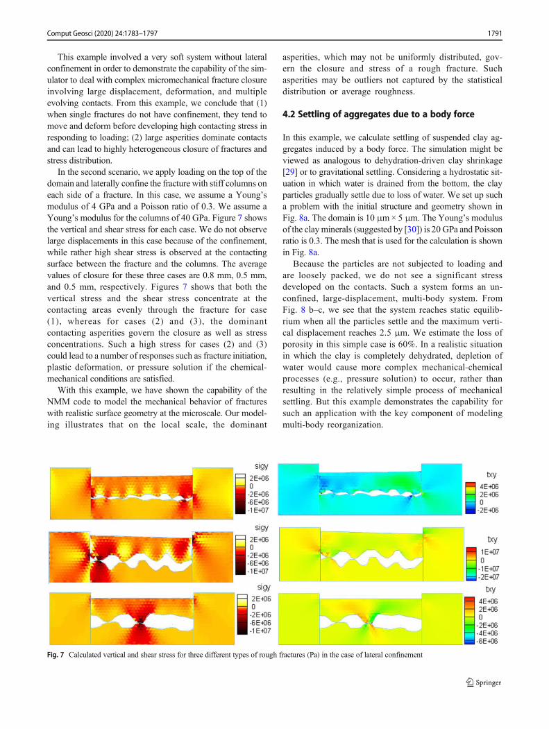
In the second scenario, we apply loading on the top of thedomain and laterally confine the fracture with stiff columns oneach side of a fracture. In this case, we assume a Young’smodulus of 4 GPa and a Poisson ratio of 0.3. We assume aYoung’s modulus for the columns of 40 GPa. Figure 7 showsthe vertical and shear stress for each case. We do not observelarge displacements in this case because of the confinement,while rather high shear stress is observed at the contactingsurface between the fracture and the columns. The averagevalues of closure for these three cases are 0.8 mm, 0.5 mm,and 0.5 mm, respectively. Figures 7 shows that both thevertical stress and the shear stress concentrate at thecontacting areas evenly through the fracture for case(1), whereas for cases (2) and (3), the dominantcontacting asperities govern the closure as well as stressconcentrations. Such a high stress for cases (2) and (3)could lead to a number of responses such as fracture initiation,plastic deformation, or pressure solution if the chemical-mechanical conditions are satisfied.

With this example, we have shown the capability of theNMM code to model the mechanical behavior of fractureswith realistic surface geometry at the microscale. Our model-ing illustrates that on the local scale, the dominant

asperities, which may not be uniformly distributed, gov-ern the closure and stress of a rough fracture. Suchasperities may be outliers not captured by the statisticaldistribution or average roughness.

4.2 Settling of aggregates due to a body force

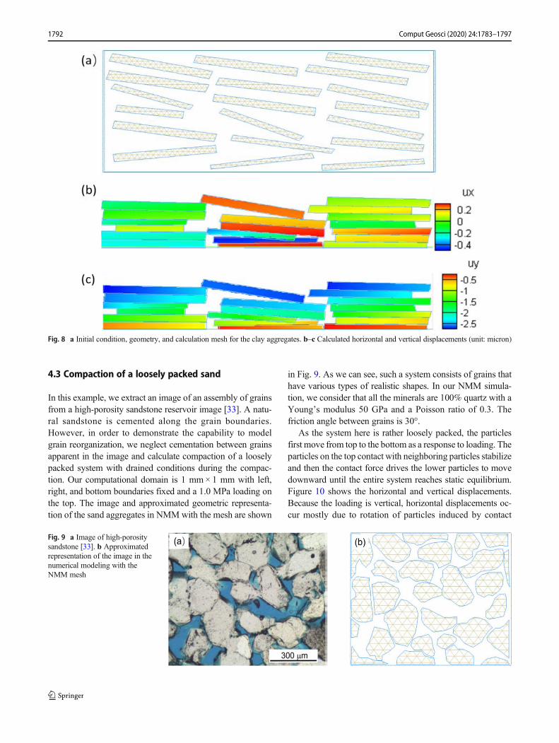
In this example, we calculate settling of suspended clay ag-gregates induced by a body force. The simulation might beviewed as analogous to dehydration-driven clay shrinkage[29] or to gravitational settling. Considering a hydrostatic sit-uation in which water is drained from the bottom, the clayparticles gradually settle due to loss of water. We set up sucha problem with the initial structure and geometry shown inFig. 8a. The domain is 10 μm× 5 μm. The Young’s modulusof the clayminerals (suggested by [30]) is 20 GPa and Poissonratio is 0.3. The mesh that is used for the calculation is shownin Fig. 8a.

Because the particles are not subjected to loading andare loosely packed, we do not see a significant stressdeveloped on the contacts. Such a system forms an un-confined, large-displacement, multi-body system. FromFig. 8 b–c, we see that the system reaches static equilib-rium when all the particles settle and the maximum verti-cal displacement reaches 2.5 μm. We estimate the loss ofporosity in this simple case is 60%. In a realistic situationin which the clay is completely dehydrated, depletion ofwater would cause more complex mechanical-chemicalprocesses (e.g., pressure solution) to occur, rather thanresulting in the relatively simple process of mechanicalsettling. But this example demonstrates the capability forsuch an application with the key component of modelingmulti-body reorganization.

Fig. 7 Calculated vertical and shear stress for three different types of rough fractures (Pa) in the case of lateral confinement

1791Comput Geosci (2020) 24:1783–1797

4.3 Compaction of a loosely packed sand

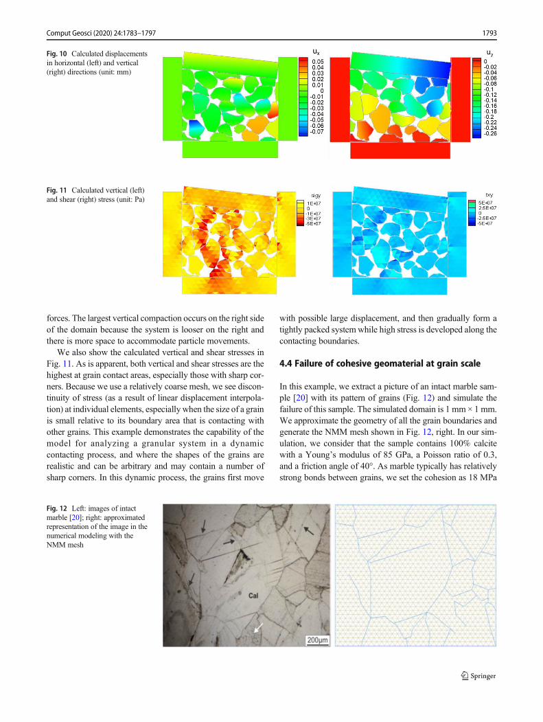
In this example, we extract an image of an assembly of grainsfrom a high-porosity sandstone reservoir image [33]. A natu-ral sandstone is cemented along the grain boundaries.However, in order to demonstrate the capability to modelgrain reorganization, we neglect cementation between grainsapparent in the image and calculate compaction of a looselypacked system with drained conditions during the compac-tion. Our computational domain is 1 mm× 1 mm with left,right, and bottom boundaries fixed and a 1.0 MPa loading onthe top. The image and approximated geometric representa-tion of the sand aggregates in NMMwith the mesh are shown

in Fig. 9. As we can see, such a system consists of grains thathave various types of realistic shapes. In our NMM simula-tion, we consider that all the minerals are 100% quartz with aYoung’s modulus 50 GPa and a Poisson ratio of 0.3. Thefriction angle between grains is 30°.

As the system here is rather loosely packed, the particlesfirst move from top to the bottom as a response to loading. Theparticles on the top contact with neighboring particles stabilizeand then the contact force drives the lower particles to movedownward until the entire system reaches static equilibrium.Figure 10 shows the horizontal and vertical displacements.Because the loading is vertical, horizontal displacements oc-cur mostly due to rotation of particles induced by contact

Fig. 9 a Image of high-porositysandstone [33]. b Approximatedrepresentation of the image in thenumerical modeling with theNMM mesh

Fig. 8 a Initial condition, geometry, and calculation mesh for the clay aggregates. b–c Calculated horizontal and vertical displacements (unit: micron)

1792 Comput Geosci (2020) 24:1783–1797

forces. The largest vertical compaction occurs on the right sideof the domain because the system is looser on the right andthere is more space to accommodate particle movements.

We also show the calculated vertical and shear stresses inFig. 11. As is apparent, both vertical and shear stresses are thehighest at grain contact areas, especially those with sharp cor-ners. Because we use a relatively coarse mesh, we see discon-tinuity of stress (as a result of linear displacement interpola-tion) at individual elements, especially when the size of a grainis small relative to its boundary area that is contacting withother grains. This example demonstrates the capability of themodel for analyzing a granular system in a dynamiccontacting process, and where the shapes of the grains arerealistic and can be arbitrary and may contain a number ofsharp corners. In this dynamic process, the grains first move

with possible large displacement, and then gradually form atightly packed systemwhile high stress is developed along thecontacting boundaries.

4.4 Failure of cohesive geomaterial at grain scale

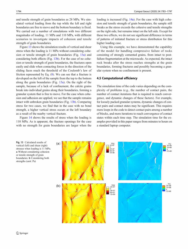
In this example, we extract a picture of an intact marble sam-ple [20] with its pattern of grains (Fig. 12) and simulate thefailure of this sample. The simulated domain is 1 mm× 1 mm.We approximate the geometry of all the grain boundaries andgenerate the NMM mesh shown in Fig. 12, right. In our sim-ulation, we consider that the sample contains 100% calcitewith a Young’s modulus of 85 GPa, a Poisson ratio of 0.3,and a friction angle of 40°. As marble typically has relativelystrong bonds between grains, we set the cohesion as 18 MPa

Fig. 11 Calculated vertical (left)and shear (right) stress (unit: Pa)

Fig. 10 Calculated displacementsin horizontal (left) and vertical(right) directions (unit: mm)

Fig. 12 Left: images of intactmarble [20]; right: approximatedrepresentation of the image in thenumerical modeling with theNMM mesh

1793Comput Geosci (2020) 24:1783–1797

and tensile strength of grain boundaries as 28 MPa. We sim-ulated vertical loading from the top while the left and rightboundaries are free to move and the bottom boundary is fixed.We carried out a number of simulations with two differentmagnitudes of loading, 11 MPa and 110 MPa, with differentscenarios to investigate impacts of cohesion and tensilestrength of grain boundaries.

Figure 13 shows the simulation results of vertical and shearstress when the loading is 11 MPa without considering cohe-sion or tensile strength of grain boundaries (Fig. 13a) andconsidering both effects (Fig. 13b). For the case of no cohe-sion or tensile strength of grain boundaries, the fractures openeasily and slide when contacting forces in the direction of thesliding faces reach the threshold of the Coulomb’s law offriction represented by Eq. (8). We can see that a fracture isdeveloped on the left of the sample from the top to the bottomalong the grain boundaries (Fig. 13a). On the right of thesample, because of a lack of confinement, the calcite grainsbreak into individual grains along their boundaries, forming agranular system that is free to move. For the case when cohe-sion and adhesion are applied, we see that the sample remainsintact with unbroken grain boundaries (Fig. 13b). Comparingstress for two cases, we find that in the case with no bondstrength, a higher vertical stress occurs at the left boundaryas a result of the nearby vertical fracture.

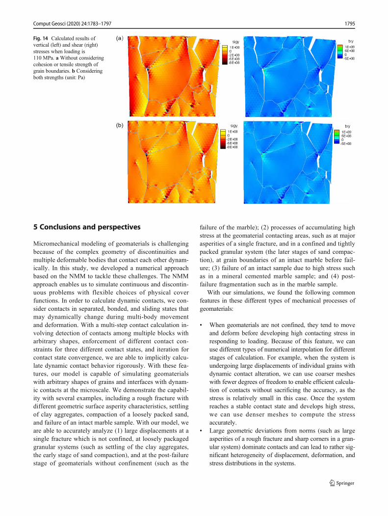
Figure 14 shows the results of stress when the loading is110 MPa. As is apparent, the fracture openings for the casewith no strength for grain boundaries are larger when the

loading is increased (Fig. 14a). For the case with high cohe-sion and tensile strength of grain boundaries, the sample stillbreaks as the stress exceeds the cohesive and tensile strengthson the right side, but remains intact on the left side. Except forthese two effects, we do not see significant difference in termsof patterns of initiated fracture or stress distribution for thishigher loading case.

Using this example, we have demonstrated the capabilityof the model for handling compressive failure of rocksconsisting of strongly cemented grains, from intact to post-failure fragmentation at the microscale. As expected, the intactrock breaks after the stress reaches strengths at the grainboundaries, forming fractures and possibly becoming a gran-ular system when no confinement is present.

4.5 Computational efficiency

The simulation time of the code varies depending on the com-plexity of problems (e.g., the number of contact pairs, thenumber of contact iterations that is required to reach conver-gence, and dynamic changes of these factors). For example,for loosely packed granular systems, dynamic changes of con-tact pairs and contact states may be significant. This requiresmore loops in the code to detect contact pairs among a numberof blocks, and more iterations to reach convergence of contactstates within each time step. The simulation time for the ex-amples provided in this paper ranges fromminutes to hours ona standard laptop computer.

Fig. 13 Calculated results ofvertical (left) and shear (right)stresses when loading is 11 MPa.a Without considering cohesionor tensile strength of grainboundaries. b Considering bothstrengths (unit: Pa)

1794 Comput Geosci (2020) 24:1783–1797

5 Conclusions and perspectives

Micromechanical modeling of geomaterials is challengingbecause of the complex geometry of discontinuities andmultiple deformable bodies that contact each other dynam-ically. In this study, we developed a numerical approachbased on the NMM to tackle these challenges. The NMMapproach enables us to simulate continuous and discontin-uous problems with flexible choices of physical coverfunctions. In order to calculate dynamic contacts, we con-sider contacts in separated, bonded, and sliding states thatmay dynamically change during multi-body movementand deformation. With a multi-step contact calculation in-volving detection of contacts among multiple blocks witharbitrary shapes, enforcement of different contact con-straints for three different contact states, and iteration forcontact state convergence, we are able to implicitly calcu-late dynamic contact behavior rigorously. With these fea-tures, our model is capable of simulating geomaterialswith arbitrary shapes of grains and interfaces with dynam-ic contacts at the microscale. We demonstrate the capabil-ity with several examples, including a rough fracture withdifferent geometric surface asperity characteristics, settlingof clay aggregates, compaction of a loosely packed sand,and failure of an intact marble sample. With our model, weare able to accurately analyze (1) large displacements at asingle fracture which is not confined, at loosely packagedgranular systems (such as settling of the clay aggregates,the early stage of sand compaction), and at the post-failurestage of geomaterials without confinement (such as the

failure of the marble); (2) processes of accumulating highstress at the geomaterial contacting areas, such as at majorasperities of a single fracture, and in a confined and tightlypacked granular system (the later stages of sand compac-tion), at grain boundaries of an intact marble before fail-ure; (3) failure of an intact sample due to high stress suchas in a mineral cemented marble sample; and (4) post-failure fragmentation such as in the marble sample.

With our simulations, we found the following commonfeatures in these different types of mechanical processes ofgeomaterials:

& When geomaterials are not confined, they tend to moveand deform before developing high contacting stress inresponding to loading. Because of this feature, we canuse different types of numerical interpolation for differentstages of calculation. For example, when the system isundergoing large displacements of individual grains withdynamic contact alteration, we can use coarser mesheswith fewer degrees of freedom to enable efficient calcula-tion of contacts without sacrificing the accuracy, as thestress is relatively small in this case. Once the systemreaches a stable contact state and develops high stress,we can use denser meshes to compute the stressaccurately.

& Large geometric deviations from norms (such as largeasperities of a rough fracture and sharp corners in a gran-ular system) dominate contacts and can lead to rather sig-nificant heterogeneity of displacement, deformation, andstress distributions in the systems.

Fig. 14 Calculated results ofvertical (left) and shear (right)stresses when loading is110 MPa. a Without consideringcohesion or tensile strength ofgrain boundaries. b Consideringboth strengths (unit: Pa)

1795Comput Geosci (2020) 24:1783–1797

& For loosely packed granular systems, large displacementsmay be the dominant response to stress. After large dis-placements and deformation, such loosely packed systemsbecome tightly packed and high stress can develop at con-tact areas.

Future work will involve combination of the NMM ap-proach with laboratory experiments for analyzing deformationand contacts of geomaterials with realistic geometric represen-tation, possibly with extension of being coupled with fluidflow, heat transfer, and chemical reaction for multiphysicsanalysis in complex geosystems at the microscale.

Acknowledgments Editorial review by Dr. Carl Steefel at Berkeley Labis greatly appreciated.

Funding information This research was supported by the USDepartmentof Energy (DOE), including the Office of Basic Energy Sciences,Chemical Sciences, Geosciences, and Biosciences Division and theOffice of Nuclear Energy, Spent Fuel and Waste DispositionCampaign, both under Contract No. DE-AC02-05CH11231 withBerkeley Lab. Additional support was from Laboratory DirectedResearch and Development (LDRD) funding from Berkeley Lab.

Open Access This article is licensed under a Creative CommonsAttribution 4.0 International License, which permits use, sharing, adap-tation, distribution and reproduction in any medium or format, as long asyou give appropriate credit to the original author(s) and the source, pro-vide a link to the Creative Commons licence, and indicate if changes weremade. The images or other third party material in this article are includedin the article's Creative Commons licence, unless indicated otherwise in acredit line to the material. If material is not included in the article'sCreative Commons licence and your intended use is not permitted bystatutory regulation or exceeds the permitted use, you will need to obtainpermission directly from the copyright holder. To view a copy of thislicence, visit http://creativecommons.org/licenses/by/4.0/.

References

1. Al-Yaarubi, A.H., Pain, C.C., Grattoni, C.A., Zimmerman, R.W.:Navier–stokes simulations of fluid flow through a rough fracture.Dynamics of fluids and transport in fractured rock. Geophys.Monograph Ser. 162, 55–64 (2005)

2. Andrade, J.E., Lim, K.W., Avila, C.F., Vlahinic, I.: Granular ele-ment method for computational particle mechanics. Comput.Methods Appl. Mech. Eng. 241, 262–274 (2012)

3. Bond, A.E., Bruský, I., Cao, T., Chittenden, N., Fedors, R.,Feng, X.T., Gwo, J.P., Kolditz, O., Lang, P., McDermott, C.,Neretnieks, I., Pan, P.Z., Šembera, J., Shao, H., Watanabe, N.,Yasuhara, H., Zheng, H.: A synthesis of approaches for model-ling coupled thermal–hydraulic–mechanical–chemical process-es in a single novaculite fracture experiment. Environ. Earth Sci.76, 12 (2017)

4. Chen, G., Ohnishi, Y., Ito, T.: Development of high-order manifoldmethod. Int. J. Numer. Methods Eng. 43, 685–712 (1998)

5. Cundall, P.A.: Formulation of a three-dimensional distinct elementmodel—part I. a scheme to detect and represent contacts in a systemcomposed of many polyhedral blocks. Int. J. Rock Mech. Min. Sci.Geomech. Abstr. 25, 107–116 (1988)

6. Fan, L., Yi, X., Ma, G.: Numerical manifold method (NMM) sim-ulation of stress wave propagation through fractured rock mass. Int.J. Comput. Methods. 5(2), 1350022 (2013)

7. He, L., An, X., Ma, G., Zhao, Z.: Development of three-dimensional numerical manifold method for jointed rock slope sta-bility analysis. Int. J. Rock Mech. Min. Sci. 64, 22–35 (2013)

8. Houlsby, G.T.: Potential particles: a method for modelling non-circular particles in dem. Comput. Geotech. 36(6), 953–959 (2009)

9. Hu, M., Rutqvist, J.: Numerical manifold method modeling ofcoupled processes in fractured geological media at multiple scales.J. Rock Mech. Geotech. Eng. (2020a). https://doi.org/10.1016/j.jrmge.2020.03.002

10. Hu, M., Rutqvist, J.: Finite volume modeling of coupled thermo-hydro-mechanical processes with application to brine migration insalt. Comput. Geosci. (2020b). https://doi.org/10.1007/s10596-020-09943-8

11. Hu, M., Wang, Y., Rutqvist, J.: Development of a discontinuousapproach for modeling fluid flow in heterogeneous media using thenumerical manifold method. Int. J. Numer. Anal. MethodsGeomech. 39, 1932–1952 (2015a)

12. Hu, M.,Wang, Y., Rutqvist, J.: An effective approach for modelingwater flow in heterogeneous media using Numerical ManifoldMethod. Int. J. Numer. Methods Fluids. 77, 459–476 (2015b)

13. Hu, M., Rutqvist, J., Wang, Y.: A practical model for flow indiscrete-fracture porous media by using the numerical manifoldmethod. Adv. Water Resour. 97, 38–51 (2016)

14. Hu, M., Wang, Y., Rutqvist, J.: Fully coupled hydro-mechanicalnumerical manifold modeling of porous rock with dominant frac-tures. Acta Geotech. 12(2), 231–252 (2017a)

15. Hu, M., Rutqvist, J., Wang, Y.: A numerical manifold methodmodel for analyzing fully coupled hydro-mechanical processes inporous rock masses with discrete fractures. Adv. Water Resour.102, 111–126 (2017b)

16. Lai, J., Wang, G., Fan, Z., Chen, J., Qin, Z., Xiao, C., Wang, S.,Fan, X.: Three-dimensional quantitative fracture analysis of tightgas sandstones using industrial computed tomography. Sci. Rep. 7,1825 (2017)

17. Ma, G., An, X., He, L.: The numerical manifold method: a review.Int. J. Comput. Methods. 7(1), 1–32 (2010)

18. Neuville, A., Flekkøy, E.G., Toussaint, R.: Influence of asperitieson fluid and thermal flow in a fracture: a coupled Lattice Boltzmannstudy. J. Geophys. Res. Solid Earth. 118, 3394–3407 (2013)

19. Ning, Y., An, X., Ma, G.: Footwall slope stability analysis with thenumerical manifold method. Int. J. Rock Mech. Min. Sci. 48, 964–975 (2011)

20. Rodríguez, P., Arab, P.B., Celestino, T.B.: Characterization of rockcracking patterns in diametral compression tests by acoustic emis-sion and petrographic analysis. Int. J. RockMech. Min. Sci. 83, 73–85 (2016)

21. Rutqvist, J.: The geomechanics of CO2 storage in deep sedimentaryformations. Int. J. Geotech. Geol. Eng. 30, 525–551 (2012)

22. Rutqvist, J., Moridis, G.: Numerical studies on the geomechanicalstability of hydrate-bearing sediments. SPE J. 14, 267–282 (2009)

23. Rutqvist, J., Zheng, L., Chen, F., Liu, H.-H., Birkholzer, J.:Modeling of coupled thermo-hydro-mechanical processes withlinks to geochemistry associated with bentonite-backfilled reposi-tory tunnels in clay formations. Rock Mech. Rock. Eng. 47, 167–186 (2014)

24. Sauer, R., Lorenzis, L.D.: An unbiased computational contact for-mulation for 3d friction. Int. J. Numer. Methods Eng. 101, 251–280(2015)

25. Shi G.: Manifold method of material analysis. Transaction of the9th army conference on applied mathematics and computing, U.S.Army Research Office (1992)

1796 Comput Geosci (2020) 24:1783–1797

26. Shi G.: Simplex integration for manifold method, FEM and DDA.Discontinuous Deformation Analysis (DDA) and Simulations ofDiscontinuous Media. TSI press. 205–262 (1996)

27. Shi, G.: Contact theory. SCIENCECHINATechnol. Sci. 58, 1450–1496 (2015)

28. Steefel, C.I.: Reactive transport at the crossroads. Rev. Mineral.Geochem. 85, 1–26 (2019)

29. Underwood, T.R., Bourg, I.: Large-scale molecular dynamics sim-ulation of the dehydration of a suspension of smectite clay nano-particles. J. Phys. Chem. C. 124, 3702–3714 (2020)

30. Vanorio, T., Prasad, M., Nur, A.: Elastic properties of dry claymineral aggregates, suspensions and sandstones. Geophys. J. Int.155, 319–326 (2003)

31. Voltolini, M., Ajo-Franklin, J.: Evolution of propped fractures inshales: the microscale controlling factors as revealed by in situ x-raymicrotomography. J. Pet. Sci. Eng. 188, 106861 (2020)

32. Wang, Y., Hu, M., Zhou, Q., Rutqvist, J.: A new second-ordernumerical manifold method model with an efficient scheme foranalyzing free surface flow with inner drains. Appl. Math. Model.40, 1427–1445 (2016)

33. Worden, R.H., Armitage, P.J., Butcher, A.R., Churchill, J.M.,Csoma, A.E., Hollis, C., Lander, R.H., Omma, J.E.: Reservoir qual-ity of clastic and carbonate rocks: analysis, modelling and predic-tion. Geol. Soc. Lond., Spec. Publ. 435, 1–31 (2018)

34. Wu, Z., Fan, L., Liu, Q., Ma, G.: Micro-mechanical modeling of themacro-mechanical response and fracture behavior of rock using thenumerical manifold method. Eng. Geol. 225, 49–60 (2017)

35. Zheng, H., Wang, F.: The numerical manifold method for exteriorproblems. Comput. Methods Appl. Mech. Eng. 364, 112968 (2020)

36. Zheng, H., Xu, D.: New strategies for some issues of numericalmanifold method in simulation of crack propagation. Int. J.Numer. Meth. Engng. 97, 986–1010 (2014)

37. Zheng, H., Zhang, P., Du, X.: Dual form of discontinuous defor-mation analysis. Comput. Methods Appl. Mech. Eng. 305, 196–216 (2016)

38. Zhuang, L., Jung, S.G., Diaz, M., Kim, K.Y., Hofmann, H., Min,K.B., Zang, A., Stephansson, O., Zimmerman, G., Yoon, J.S.:Laboratory true triaxial hydraulic fracturing of granite under sixfluid injection schemes and grain-scale fracture observations.Rock Mech. Rock. Eng. (2020). https://doi.org/10.1007/s00603-020-02170-8

39. Zou, L., Jing, L., Cvetkovic, V.: Roughness decomposition andnonlinear fluid flow in a single rock fracture. Int. J. Rock Mech.Min. Sci. 75, 102–118 (2015)

40. Puso, M.A., Laursen, T.A.: A mortar segment-to-segment contactmethod for large deformation solid mechanics. Comput. MethodsAppl. Mech. Engrg. 193, 601–629 (2004)

Publisher’s note Springer Nature remains neutral with regard to jurisdic-tional claims in published maps and institutional affiliations.

1797Comput Geosci (2020) 24:1783–1797