Embed Size (px)
Citation preview

MICRO/MACROSCOPIC FLUID FLOW IN OPEN CELL
FIBROUS STRUCTURES
by
Ali Tamayol M.Sc., Sharif University of Technology, 2005
B.Sc. (Mechanical Engineering), Shiraz University, 1999
DISSERTATION SUBMITTED IN PARTIAL FULFILLMENT OF THE REQUIREMENTS FOR THE DEGREE OF
DOCTOR OF PHILOSOPHY
In the Program of Mechatronic Systems Engineering
Faculty of Applied Science
© Ali Tamayol 2011
SIMON FRASER UNIVERSITY
Summer 2011
All rights reserved. However, in accordance with the Copyright Act of Canada, this work may be reproduced, without authorization, under the conditions for Fair Dealing.
Therefore, limited reproduction of this work for the purposes of private study, research, criticism, review and news reporting is likely to be in accordance with the law,
particularly if cited appropriately.

ii
Approval
Name: Ali Tamayol
Degree: Doctor of Philosophy (PhD)
Title of Thesis: MICRO/MACROSCOPIC FLUID FLOW IN OPEN CELL FIBROUS STRUCTURES
Examining Committee:
Chair:
Name: Martin Ordonez Defense Chair Assistant Professor
Name: Majid Bahrami Senior Supervisor Assistant Professor
Name: Bonnie L. Gray Supervisor Associate Professor
Name: Michael Eikerling Supervisor Associate Professor
Name: Behrad Bahrayni Internal Examiner Assistant Professor
Name: Sushanta K. Mitra External Examiner Associate Professor University of Alberta
Date Defended/Approved: July 14, 2011
iii
Abstract
Fibrous porous materials are involved in a wide range of applications including
composite fabrication, filtration, compact heat exchangers, fuel cell technology, and
tissue engineering to name a few. Fibrous structures, such as metalfoams, have unique
characteristics such as low weight, high porosity, high mechanical strength, and high
surface to volume ratio. More importantly, in many applications the fibrous
microstructures can be tailored to meet a range of requirements. Therefore, fibrous
materials have the potential to be used in emerging sustainable energy conversion
applications.
The first step for analyzing transport phenomena in porous materials is to
determine the micro/macroscopic flow-field inside the medium. In applications where the
porous media is confined in a channel, the system performance is tightly related to the
flow properties of the porous medium and its interaction with the channel walls, i.e.,
macroscopic velocity distribution.
Therefore, the focus of the study has been on:
developing new mechanistic model(s) for determining permeability and
inertial coefficient of fibrous porous materials;

iv
investigating the effects of microstructural and mechanical parameters
such as porosity, fiber orientation, mechanical compression, and fiber
distribution on the flow properties and pressure drop of fibrous structures;
determining the macroscopic flow-field in confined porous media where
the porous structure fills the channel cross-section totally or partially.
A systematic approach has been followed to study different aspects of the flow
through fibrous materials. The complex microstructure of real materials has been
modelled using unit cells that have been assumed to be repeated throughout the media.
Implementing various exact and approximate analytical techniques such as integral
technique, point matching, blending rules, and scale analysis the flow properties of such
media have been modelled; the targeted properties include permeability and inertial
coefficient. In addition, fluid flow through microchannels, fully and partially filled with
porous media, has been modelled using a volume-averaged equation, which is a novel
approach in Microfluidics.
To verify the developed models, several testbeds have been designed and
experimental studies have been conducted with various fluids and porous materials. The
proposed models have been verified with the measured data and the experimental results
reported by others.
Keywords: Fibrous porous media; Permeability; Inertial coefficient; Theoretical
modeling; Numerical simulation; Experimental verification; Confined porous media;
Metalfoams; Gas diffusion layers; Sustainable energy; Transport phenomena.

v
Executive Summary
Fibrous porous materials are involved in a wide range of applications including
composite fabrication, filtration, compact heat exchangers, paper production, fuel cell
technology, and tissue engineering. In comparison with packed beds of spherical
particles, fibrous structures have superior characteristics such as low weight, high
porosity, high mechanical strength, and high surface to volume ratio. More importantly,
in many applications the fibrous microstructures can be tailored to meet a range of
requirements. Therefore, fibrous materials have the potential to be used in emerging
sustainable energy conversion applications.
Despite numerous existing studies, the transport characteristics of fibrous media
are not fully understood. This is one of the several reasons for the current intense
worldwide efforts to investigate transport phenomena in such structures. The first step is
to determine the macroscopic flow-field inside and at the interface of the medium. As
such, the motivation of the present study is to determine pressure drop and both
microscopic and macroscopic flow-field in fibrous materials with focus on the following
applications:
Fuel cell technology: Gas diffusion layer (GDL) of polymer electrolyte
membrane fuel cells (PEMFCs) is a fibrous porous material with a planar structure. In
addition to mechanical support of the membrane, GDL allows transport of reactants,
products, and electrons from the bipolar plate towards the catalyst layer and vice versa.

vi
In-plane and through-plane gas permeability of GDL affects the PEM fuel cell
performance and plays a key role in the design and optimization process of PEMFCs.
Compact heat exchangers: Open cell metalfoams, formed by small ligaments
creating interconnected dodecahedral-like cells, have unique features including: excellent
surface-area-to-volume ratio, high temperature tolerance, low density (typically with
specific gravity of 0.1), high mechanical strength, and corrosion resistance in comparison
with regular steel fins. Foams can be constructed from a wide variety of materials
including metals (aluminum, nickel, copper, iron, and steel alloys), polymers, and carbon.
As a result of recent decrease in production costs, metalfoams have received a special
attention as a candidate for designing compact heat exchangers in the past decade. In-
depth understanding of flow in metalfoams is important for any thermal and heat
exchanger effectiveness analysis
Filtration: Filtration is a common way for separating particles from the bulk
fluid. Usually, a porous structure or membrane is used for trapping the targeted particles.
The microstructure of a majority of filtering media is fibrous. An understanding of flow-
field and the resulting pressure drop is crucial in the design and optimization of filtration
systems.
The morphological parameters that are commonly used to describe porous media
include: 1) porosity that is the ratio of the void volume to the total volume and 2) fiber
diameter. However, in special cases, other parameters have also been used, e.g., the
polytetrafluoro ethylene (PTFE) content for GDLs and pore density, number of pores per
unit length, typically expressed in pores per inch (PPI), for metalfoams.

vii
In many applications, the porous media is embedded inside a channel (confined
porous media), occupying the entire or part of the channel’s cross-section.
Mini/microchannels filled with porous media (micro-porous channels) are currently used
in filtration, detection of particles, compact heat exchanger design, fuel cell technology,
and tissue engineering. Such structures have also been used in biological and life sciences
for analyzing biological materials such as proteins, DNA, cells, embryos, and chemical
reagents. The performance of the abovementioned systems is tightly linked to the flow
properties of the porous media and its interaction with the channel walls.
Objectives
The main goals of the proposed research can be summarized as:
Developing new mechanistic model(s) for the permeability and the inertial
coefficient of fibrous porous materials with 1, 2, and 3 directional
microstructures.
Investigating the effects of microstructural and mechanical parameters
such as porosity, fiber orientation, mechanical compression, and fiber
distribution on the flow properties and pressure drop of fibrous structures.
Determining the macroscopic flow-field and the resulting pressure drop in
confined porous media, where the microstructure totally or partially fills
the channel’ cross-section.
The developed models will serve as a powerful tool in design and optimization
process for engineers and scientist investigating a variety of areas including fuels cell
technology, compact heat exchangers, tissue engineering, and filtration.

viii
Methodology
In this study, a systematic approach is adopted to study various aspects of fluid
flow through fibrous materials. The problem is divided into smaller parts where
analytical and experimental studies are carried out; Figure 1 shows the road map and the
deliverables of the thesis.
The focus of the present study is on developing fundamental models that can
accurately predict the flow properties of fibrous porous media. The developed
fundamental models can be tailored for each specific application through implementing
specific morphological parameters. The random, complex microstructure of real porous
materials is modeled using unit cells that are assumed to be repeated throughout the
volume. Analysis of the considered unit cells enables one to develop compact solutions
with a reasonable accuracy. Then, based on the microstructure and flow characteristics,
various exact and approximate analytical techniques such as integral technique, point
matching, blending rules, and scale analysis are employed to predict the pressure drop
and as a result the permeability. Unlike the majority of the existing studies in the
literature, the proposed models are applicable to various materials without a need to find
a “tuning parameter”. In the moderate Reynolds number flows, numerical simulations are
performed to propose accurate and compact relationships for predicting the inertial
coefficient in the considered microstructures.
To verify the developed models and proposed correlations, three new
experimental test beds have been designed and built at Simon Fraser University to
conduct experimental studies with various fluids and materials at different scales.

ix
Although the thrust of the present study is to determine the flow properties of
GDLs and metalfoams, the reported results and the approach are applicable to any other
fibrous material with similar microstructures.
This dissertation is divided into 5 chapters and 3 appendices. Chapter 1 includes
an introduction including a theoretical background on flow through fibrous media. A
critical review of the pertinent literature is presented is Chapter 2 to justify the necessity
for the research. Chapter 3 includes all the microscopic analysis for determining the flow
properties (permeability and inertial coefficient) of fibrous structures. Boundary effects
on macroscopic velocity distribution and pressure drop in channels partially and fully
filled with porous media is investigated in Chapter 4. Summary and conclusions of the
dissertation is presented in Chapter 5. This chapter also includes the possible
continuations of the current dissertation. Appendix A includes all the experimental and
numerical data collected from various sources and used in the dissertation. Details of the
experimental measurements performed in the dissertation are listed in Appendix B. More
details on the numerical simulations performed in the dissertation are provided in
Appendix C.

x
Macroscopic flow in channels filled with porous media
Partially filled channels
Fully filled channels
Solutions for macroscopic velocity distribution and pressure drop in channels fully/partially filled with porous media
Model(s) for permeability and inertial coefficient of ordered 1D, 2D, 3D, and random structures.
Microscopic flow (flow properties)
Creeping flow Re <1
Inertial flow 1 < Re < 1000
2D 3D1D
Considered geometries
Figure 1: The present research project road map and deliverables.

xi
Dedication
To my family and
my wife
Neda

xii
Acknowledgements
I would like to thank my senior supervisor, Dr. Majid Bahrami, for his support,
guidance, and insightful discussions throughout this research. It was a privilege for me to
work with him and learn from his experience.
I am also indebted to Drs. Bonnie Gray, Nedjib Djilali, and Kamel Hooman for
the useful discussions which helped me to define the project and to pursue its goals;
specially, Dr. Bonnie Gray who allowed me to use MIL’s microfabrication facility. It has
been a great opportunity for me to collaborate with them.
I would like to thank my colleagues and lab mates at Multiscale Thermofluidic
Laboratory for Sustainable Energy Research at Simon Fraser University. Their helps,
comments, and assistance played an important role in the development of this
dissertation. In particular, I want to thank Kelsey Wong, Mohsen Akbari, Fraser
Macgregor, Remington Bouher, Ehsan Sdeghi, Ajit Khosla, and Peyman Taheri.
I have received financial supports from Natural Sciences and Engineering
Research Council (NSERC) of Canada, British Columbia Innovation Council (BCIC),
Kaiser Foundation, University of Victoria, and Simon Fraser University.
I have to thank my family that have endlessly encouraged and supported me
during all the aspects of my life. Preparing this thesis was not possible without the
sacrifice and understanding of my wife, Neda. Sharing my life with her made this
stressful period, pleasant and enjoyable.

xiii
Contents
Approval ................................................................................................................. ii
Abstract .................................................................................................................. iii
Executive Summary ................................................................................................ v
Dedication .............................................................................................................. xi
Acknowledgements ............................................................................................... xii
Contents ............................................................................................................... xiii
List of Figures ..................................................................................................... xvii
Glossary .............................................................................................................. xxv
1: Introduction ......................................................................................................... 1
2: Literature Review ............................................................................................... 9
2.1 Creeping flow through fibrous media ....................................................... 9
2.1.1 Capillaric models and pore network modeling approach .................... 9
2.1.2 Deterministic approach ..................................................................... 12
2.1.3 Blending rules (Mixing rules) ............................................................ 22
2.1.4 Analogy of hydraulic permeability with other diffusive properties ... 23
2.1.5 Experimental studies .......................................................................... 24
xiv
2.2 Inertial flow regime (moderate Reynolds numbers) ............................... 25
2.2.1 Theoretical studies ............................................................................. 26
2.2.2 Experimental studies (moderate Reynolds numbers) ........................ 29
2.3 Flow through channels partially-/fully-filled with porous media ........... 30
2.4 Comparison of the existing models with experimental data ................... 32
2.5 Modeling road map ................................................................................ 37
3: Flow properties of fibrous structures (microscopic analyses) .......................... 39
3.1 Permeability of 1D touching fibers ......................................................... 39
3.2 Determination of the normal permeability of square fiber arrangements
(integral technique) ....................................................................................................... 41
3.3 Parallel permeability of ordered arrangements ....................................... 48
3.3.1 Numerical simulations ....................................................................... 54
3.3.1 Parallel permeability .......................................................................... 55
3.4 Blending methods for permeability of complex fibrous media ............... 61
3.4.1 In-plane permeability of GDLs (2D materials) .................................. 61
3.4.2 In-plane permeability of 3D fibrous materials ................................... 67
3.5 Transverse permeability of fibrous media: An scale analysis approach . 69
3.5.1 Tortuosity factor................................................................................. 72
3.5.2 Experimental study ............................................................................ 73

xv
3.5.3 Results and discussion ....................................................................... 76
3.6 Through-plane permeability of carbon papers ........................................ 84
3.6.1 Experimental Approach ..................................................................... 85
3.6.2 Theoretical Model .............................................................................. 91
3.6.3 Comparison of experimental and theoretical results .......................... 93
3.7 Effect of microstructure on the flow properties of fibrous media ........... 96
3.7.1 Experimental approach ...................................................................... 98
3.7.2 Numerical procedure ........................................................................ 100
3.7.3 Comparison of the numerical results with existing data in the
literature 102
3.7.4 Effects of microstructure on flow properties ................................... 105
4: Macroscopic Flow in confined porous media ................................................. 109
4.1 Pressure drop in microchannels filled with porous media .................... 109
4.2 Experimental procedure ........................................................................ 112
4.2.1 Microfabrication .............................................................................. 112
4.2.1.3 Analysis of experimental data ....................................................... 117
4.2.2 Comparison of the model with the experimental data ..................... 119
4.2.3 Numerical simulations ..................................................................... 120
4.2.4 Parametric study............................................................................... 123

xvi
4.3 Flow in channels partially filled with porous media ............................. 125
4.3.1 Solution development ...................................................................... 127
4.3.2 Comparison with experimental data ................................................ 129
4.3.3 Numerical simulations ..................................................................... 129
5: Conclusions and Future Work ........................................................................ 134
5.1 Future plan ............................................................................................. 136
6: References ................................................................................................. 137
Appendix A: experimental data collected from different sources ...................... 155
Appendix B: Details of The experimental measurements carried out in the
dissertation ...................................................................................................................... 162
Appendix C: Details of the numerical simulations performed in the dissertation
......................................................................................................................................... 169

xvii
List of Figures
Figure 1: The present research project road map and deliverables. ........................ x
Figure 2: Scanning electron micrograph (SEM) of fibrous media in different
applications a) electrospun fibrous scaffold for tissue engineering [10], b) aluminum
foam, and c) Toray carbon paper (GDL). ........................................................................... 2
Figure 3: Structures with different fibers orientation; a) one direction (1D), b) two
directional (2D), and c) three directional (3D). .................................................................. 3
Figure 4: a) Schematic of different layers in a fuel cell, b) channel-to-channel
convection, and c) in-plane flow inside GDL in the flow direction. .................................. 8
Figure 5: Schematic of capillary networks. .......................................................... 12
Figure 6: Schematic of the swarm theory approach. ............................................. 22
Figure 7: The blending technique concept for 2D structures. ............................... 23
Figure 8: Comparison of the existing models for transverse (normal) flow
permeability of square arrangements with experimental data. ......................................... 34
Figure 9: Comparison of the existing models for through-plane flow through two
directional (2D) structures with experimental data. .......................................................... 34
Figure 10: Comparison of the existing models for in-plane flow through two
directional (2D) structures with experimental data. .......................................................... 35

xviii
Figure 11: Comparison of the existing models for three directional (3D) structures
with experimental data. ..................................................................................................... 35
Figure 12: Comparison of the existing models for metalfoams a) Dukhan [98] and
b) Bonnet at al. [97] with experimental data. .................................................................... 36
Figure 13: The modeling road map of the present dissertation. ........................... 38
Figure 14: Rectangular arrangement of cylinders and the considered unit cell. ... 42
Figure 15: Comparison of the present model for permeability of square arrays of
fibers with experimental data. ........................................................................................... 46
Figure 16: a) A typical numerical grid and the boundary conditions used in the
analysis for = 0.65, b) comparison of the present numerical and the experimental data
for the velocity profiles in normal flow and = 0.9. ........................................................ 47
Figure 17: Comparison of the present numerical and parabolic velocity profiles in
normal flow, = 0.9. ........................................................................................................ 48
Figure 18: Unit cell for a) square, b) staggered, and c) hexagonal arrangements. 50
Figure 19: A typical numerical grid used in the numerical analysis a square
arrangement with = 0.9. ................................................................................................. 55
Figure 20: a) analytical velocity contours, Eq. (39), b) numerical velocity
contours, and c) analytical velocity distribution for a square arrangement with = 0.9. 56
Figure 21: Present velocity distributions for staggered arrangement of cylinders
with = 0.45 a) analytical, Eq. (39), and b) numerical. ................................................... 57

xix
Figure 22: Comparison of the proposed model for parallel permeability of square
arrangements of cylinders, experimental and numerical data, and other existing models.
........................................................................................................................................... 58
Figure 23: Comparison of the proposed model, an experimental data point
(touching limit), and other existing models, staggered arrangement. ............................... 59
Figure 24: Comparison of the proposed model with other existing models,
hexagonal arrangement. .................................................................................................... 60
Figure 25: Effect of cell arrangement on the parallel permeability of ordered
arrays of fibers. ................................................................................................................. 60
Figure 26: SEM image of Toray 90 carbon paper used as GDL in PEMFCs. ...... 61
Figure 27: Proposed periodic geometry used for modeling GDLs (2D structures).
........................................................................................................................................... 62
Figure 28: The blending technique concept for GDLs (2D structures). ............... 63
Figure 29: Comparison of different blending models with the bounds for
2/totnormpar . ..................................................................................................... 64
Figure 30: Comparison of the proposed blending model and experimental data. 65
Figure 31: Comparison of present model with other existing correlations for the
in-plane permeability of fiber mats. .................................................................................. 66
Figure 32: Proposed Simple cubic arrangement for modeling 3D (non-planar)
fibrous structures. .............................................................................................................. 67
xx
Figure 33: The blending technique concept for 3D fibrous structures. ................ 68
Figure 34: Comparison of present model with other existing correlation for 3D
structures. .......................................................................................................................... 68
Figure 35: Considered unit cells for ordered 1D structures: a) square, b) staggered,
and c) hexagonal arrays of cylinders. ............................................................................... 69
Figure 36: The 2D unit cell considered in the present study. ............................... 70
Figure 37: 3D structures; a) metalfoam, a real structure (scale bar is equal to
500 m ); b) simple cubic arrangement, modeled unit cell used in the present analysis. .. 71
Figure 38: The gravity driven test bed and the tested samples: a) actual test setup,
b) schematic, c) a sample of tube banks, and d) a sample of aluminum foam. ................ 77
Figure 39: measured pressure gradients for samples of a) tube bank with square
fiber arrangement, b) tube bank with staggered fiber arrays, and c) metalfoams. ............ 78
Figure 40 : Comparison of the proposed model for square arrangements with
experimental data measured in the present study or reported by others. .......................... 79
Figure 41: Comparison of the proposed model and current experimental data with
numerical results of Higdon and Ford [40] for staggered arrangements. ......................... 80
Figure 42: Comparison of the present model, models of Van Doormaal and
Pharoah [51] and Tomadakis and Robertson [11] with experimental data for transverse
permeability of 2D structures. ........................................................................................... 83
xxi
Figure 43: Comparison of the proposed model for 3D structures, models of
Jackson and James [54] and Tomadakis and Robertson [11], present experimental results
and data reported by others. .............................................................................................. 84
Figure 44: SEM Images: a) TGP 120 with 5% PTFE content; b) SGL Sigracet
10AA; c) compressed TGP 120 with 5% PTFE content................................................... 87
Figure 45: The air permeability test bed: a) schematic of the apparatus (exploded
view) b) actual test setup. .................................................................................................. 89
Figure 46: Measured pressure drops for samples of compressed TGP-H-120. .... 90
Figure 47: Effect of compression ratio, 0/ ttcomp on the variation of permeability.
........................................................................................................................................... 94
Figure 48: Comparison of the proposed model with the experimental data for
compressed GDLs measured in the present study or collected from various sources. ..... 94
Figure 49: Effect of PTFE content on the through-plane permeability of two set of
TGP-H-120 samples with various PTFE contents. ........................................................... 95
Figure 50: Comparison of the proposed model with the experimental data for
TGP-H-120 with various PTFE contents. ......................................................................... 96
Figure 51: Measured values of dxdpUD //1 for the samples of tube bank with
square fiber arrangement. ................................................................................................ 100
Figure 52: Comparison between the present numerical results, collected
experimental results, and data from various sources, for normal flow through square fiber
arrays. .............................................................................................................................. 104
xxii
Figure 53: Comparison between the present numerical and experimental results
for Forchheimer coefficient with experimental and numerical data of others. ............... 104
Figure 54: Comparison between the present numerical results for permeability of
simple cubic arrangements with existing numerical and experimental data of 3D
materials. ......................................................................................................................... 106
Figure 55: Comparison of numerical values of dimensionless permeability of
fibrous media with Ergun equation. ................................................................................ 106
Figure 56: Comparison of numerical values of Forchheimer coefficient of fibrous
media with Ergun equation. ............................................................................................ 107
Figure 57: Structure of the considered micro-porous channels a) the schematic, b)
a fabricated sample. ........................................................................................................ 110
Figure 58: Schematic of the simplified 2D geometry. ........................................ 112
Figure 59: Fabrication process steps for SU-8 micromold preparation via
photopatterning of SU-8 100 epoxy-based photopolymer: a) UV exposure, b) making the
mold, c) pouring liquid PDMS, and d) plasma bonding and making the channels. ....... 114
Figure 60: Rough surface of the fabricated cylinders, Sq 04-400 (1). ................ 115
Figure 61: Schematic of the experimental setup for testing pressure drop in micro-
porous channels. .............................................................................................................. 117
Figure 62: Channel pressure drop versus flow rate for Sq-0.4-400 (1), Sq-0.4-400
(2), and Sq-0.7-100. Lines show the theoretical values of pressure drop predicted by Eq.
(75) and symbols show the experimental data. ............................................................... 121

xxiii
Figure 63: Channel pressure drop versus flow rate for Sq-0.9-50 and Sq-0.95-50.
Lines show the theoretical values of pressure drop predicted by Eq. (75) and symbols
show the experimental data. ............................................................................................ 121
Figure 64: The considered unit cell and produced numerical grid for modeling of
sample Sq-04-400(2). ...................................................................................................... 122
Figure 65: Experimental, numerical, and theoretical values of channel pressure
drop predicted by Eq. (75) versus flow rate for Sq-0.4-400 (1), Sq-0.4-400 (2), and Sq-
0.7-100. ........................................................................................................................... 124
Figure 66: Experimental, numerical, and theoretical values of channel pressure
drop predicted by Eq. (75) versus flow rate for Sq-0.9-50 and Sq-0.95-50. .................. 124
Figure 67: Dimensionless pressure drop versus Darcy number squared. ........... 125
Figure 68: a) and b) Flow through channels partially filled with arrays of
cylinders, c) simplified 2D geometry. ............................................................................. 126
Figure 69: Comparison of the velocity distribution reported by Arthur et al. [115]
and the theoretical predictions by Eqs. (51) and (89). .................................................... 130
Figure 70: a) The considered geometry and b) the produced numerical grid for
modeling of sample with =0.4. .................................................................................... 131
Figure 71: Comparison of the volume averaged (Eqs. (51) and (89)) and actual
dimensionless velocity distributions in the channel filled with porous media with =0.7.
......................................................................................................................................... 132

xxiv
Figure 72: Comparison of the volume averaged (Eqs. (51) and (89))and actual
dimensionless velocity distributions in the channel filled with porous media with =0.9.
......................................................................................................................................... 133
Figure 73: Effects of porosity on the dimensionless microscopic velocity
distribution through the channels partially filled with porous media. ............................ 133
Figure 74: Developed velocity profiles in the inlet and outlet of the fourth unit cell
with =0.9. ..................................................................................................................... 170
Figure 75: The pressure drop over a unit cell with =0.9 calculated with different
number of grids. .............................................................................................................. 171
Figure 76: Comparison between the present numerical results and experimental
data, normal flow through square arrays of cylinders. .................................................... 171
Figure 77: The pressure drop over a length of 2cm for square arrays of cylinders
with d= 1 cm and =0.9 calculated with different number of grids. ............................. 173
Figure 78: Comparison between the present numerical results, experimental data,
and the numerical results of Sangani and Yao [39] for parallel permeability of square
arrays of cylinders. .......................................................................................................... 173
Figure 79: Typical computational domain used for modeling of flow a) through
simple cubic; b) parallel to 2D; c) transverse to 2D fibrous structures. ......................... 176
Figure 80: The pressure drop over a unit cell of simple cubic arrays of cylinders
with d= 1 cm and S = 4 cm for two different Reynolds numbers, calculated with different
number of grids. .............................................................................................................. 177

xxv
Glossary
1D One directional
2D Two directional
3D Three directional
A Pore cross-sectional area (normal to flow), 2m
d Fiber diameter, m
HD Hydraulic diameter of the pore, m
f Fanning friction coefficient
GDL Gas diffusion layer
F Formation factor
h Microchannel depth, m
pI Polar moment of inertia of pore cross-section, 4m
*pI Dimensionless polar moment of inertia of pore cross-section,
2* / AII pp

xxvi
K Permeability, 2m
*K Non-dimensional permeability, 2* / dKK
0k Shape factor
(.)0K Modified second kind Bessel function
(.)1K Modified second kind Bessel function
kk Kozeny constant
eqK Equivalent permeability of fiber mixtures, 2m
L Sample length, m
eL Effective length, m
Unit cell length in Eq. (3), m
MEA Membrane electrode assembly
MF Metalfoam
P Pressure, 2/ mN

xxvii
PEMFC Polymer electrolyte membrane fuel cell
PTFE Polytetrafluoro ethylene
Q Volumetric flow rate, sm /3
Re Reynolds number based on fiber diameter, /Re dUD
r Coordinate system, m
S Distance between adjacent fibers in square arrangement, m
xS Distance between adjacent fibers in rectangular unit cell in x-
direction, m
yS Distance between adjacent fibers in rectangular unit cell in y-
direction, m
SEM Scanning electron micrograph
u Velocity component, sm /
bu Velocity at the border of unit cell, sm /
intu Interface velocity, sm /
DU Volume-averaged superficial velocity, sm /

xxviii
intDU Interface volume-averaged superficial velocity, sm /
pu Seepage velocity, sm /
v Velocity component, sm /
w Velocity component, sm /
W Microchannel width, m
x Coordinate system, m
y Coordinate system, m
z Coordinate system, m
Greek symbols
Constant in Eq. (34)
Inertial coefficient, 1m
Distance between surfaces of adjacent fibers, m
Porosity
Microchannel cross-section aspect ratio
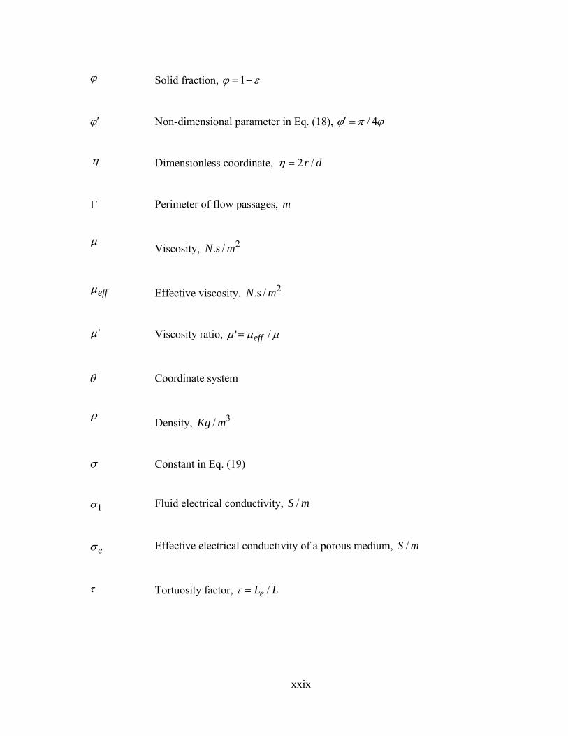
xxix
Solid fraction, 1
Non-dimensional parameter in Eq. (18), 4/
Dimensionless coordinate, dr /2
Perimeter of flow passages, m
Viscosity, 2/. msN
eff Effective viscosity, 2/. msN
' Viscosity ratio, /' eff
Coordinate system
Density, 3/ mKg
Constant in Eq. (19)
1 Fluid electrical conductivity, mS /
e Effective electrical conductivity of a porous medium, mS /
Tortuosity factor, LLe /
1
1: INTRODUCTION
A volume, partly occupied by a permeable solid or semi-solid phase while the rest
is void or occupied by one or several fluids, is called a porous medium [1]. The solid
phase can either form a consolidate matrix, e.g., metalfoams, sponges, or be distributed in
the fluid phase, e.g., particulate mixtures and granular materials. According to this
definition, porous media involve in a diverse range of natural and industrial systems.
Consequently, transport phenomena in porous media have been the focus of numerous
studies since the 1850s, which indicates the importance of this topic. Most of these
studies; however, dealt with low and medium porosity structures such as granular
materials and packed beds of spherical particles.
When the solid particles have a cylindrical shape or the solid matrix is formed by
high aspect ratio ligaments, the material is called a fibrous porous medium. Fibrous
networks can form mechanically stable geometries with high porosity, the ratio of the
void volume to the total volume up to 0.99 [2]. Moreover, these fibrous structures feature
low-weight, high surface-to-volume ratio, high flow conductivity, high heat transfer
coefficient, and high ability to mix the passing fluid [3]. Many natural and industrial
materials involved in physiological systems [4], filtration [5], composite fabrication [6],
compact heat exchangers [2, 3], paper production [7], and fuel cell technology [8, 9] have
a fibrous structure, see Figure 2. As shown in Figure 3, based on the orientation of the
fibers in space, fibrous structures can be categorized into three different groups:

2
(a)
(b)
(c)
Figure 2: Scanning electron micrograph (SEM) of fibrous media in different applications a) electrospun fibrous scaffold for tissue engineering [10], b) aluminum foam, and c) Toray carbon
paper (GDL).
one-directional (1D) such as tube banks where the axes of fibers are
parallel to each other;

3
two-directional (2D), e.g., gas diffusion layer (GDL) of fuel cells, where
the fibers axes locate on planes parallel to each other, with an arbitrary
distribution and orientation on these planes;
three-directional (3D) including metalfoams where their axes are
randomly positioned and oriented in any given volume. With the
exception of the 3D structures, the rest are anisotropic, i.e., the transport
properties are direction dependent [11].
Investigation of the transport properties of these materials dates back to 1940s for
evaluating properties of fibrous filters, and 1980s for composite fabrication. Development
of new materials for novel applications such as fuel cell technology and compact heat
exchangers has motivated researchers to investigate the transport properties of such
media.
Proton exchange membrane fuel cells (PEMFCs) have shown the potential to be
commercialized as green power sources in automotive, electronics, portables, and
(a) (b) (c)
Figure 3: Structures with different fibers orientation; a) one direction (1D), b) two directional (2D), and c) three directional (3D).
4
stationary applications [12]. PEMFCs complete an electrochemical reaction to combine
hydrogen and oxygen releasing heat, water, and electricity which can be used for a
variety of application. The membrane electrode assembly (MEA) is the heart of a
PEMFC. MEA is comprised of a membrane, loaded by catalyst layers on each side,
which is sandwiched between two porous layers named gas diffusion layers (GDLs) [12].
In addition to mechanical support of the membrane, GDL allows transport of reactants,
products, and electrons from the bipolar plate towards the catalyst layer and vice versa.
Therefore, thermophysical properties of GDLs such as gas and water permeability,
thermal, and electrical conductivity affect the PEMFC performance and reliability by
affecting reactant access and heat and product removal from catalyst layers [13, 14].
An in-depth knowledge of the variation of these thermophysical properties with
operating condition and microstructure is important in designing more reliable and
efficient PEMFCs. The important parameters that have been used to describe carbon
papers used as GDLs are: 1) porosity, (defined as the void to the total volume ratio), 2)
fiber diameter, 3) the polytetrafluoro ethylene (PTFE) content of the material.
Improving the thermal performance of thermal management systems by designing
more efficient heat exchangers currently receives an intense attention worldwide. In the
past decade, as a result of the decrease in the production cost and the unique
thermophysical properties, metalfoams have received a special attention [2]. Open cell
metalfoams consist of small ligaments forming interconnected dodecahedral-like cells,
see Figure 2. The shape and size of these open cells vary throughout the medium which
make the structure random and in some cases anisotropic. The geometrical parameters

5
that are reported by manufacturers are: 1) porosity, , 2) fiber diameter, and 3) pore
density, number of pores per unit length, typically expressed in pores per inch (PPI).
These structures can be constructed from a wide variety of materials including metals
(aluminum, nickel, copper, iron, and steel alloys), polymers, and carbon.
Determining the relationship between flow and the resulting pressure drop in
fibrous porous materials is the first step in the analysis of transport phenomena in porous
media. The complex geometry and randomness of porous materials makes developing
exact pore-scale velocity distribution highly unlikely. From an engineering view point,
however, it usually suffices to predict the macroscopic or volume averaged velocity
rather than details of pore scale velocity distribution. As a result, the transport equations
that are used in the design and analysis of fibrous systems are the volume averaged forms
of the conventional equations.
In the creeping flow regime, according to the Darcy equation the relationship
between the volume averaged velocity through porous media, DU , and the pressure drop
is linear [1]:
DUKdx
dP
(1)
where K is the permeability and is the fluid viscosity. The permeability can be
interpreted as the flow conductance of a porous medium for a Newtonian fluid [15]. In
higher Reynolds numbers, the relationship between the flow and pressure drop becomes
nonlinear and a modified Darcy equation is used [1]:

6
2DD UU
Kdx
dP
(2)
where is the inertial coefficient. However, one needs to know K and prior to using
Eqs. (1) and (2). For a fibrous medium, the flow coefficients depend on the geometrical
parameters of the solid matrix including porosity, fiber diameter, fiber shape, fiber
distribution in space, fiber orientation relative to flow direction, and surface
characteristics of the solid phase such as roughness and its behavior when in contact with
the fluid, e.g., hydrophobicity.
The flow coefficients of a porous material are determined either experimentally or
through pore scale analysis of the porous media (determining the detail velocity
distribution and finding the resulting pressure drop) where both are time consuming and
expensive tasks. As a result, having general model(s) or correlation(s) that can accurately
estimate the flow properties of different fibrous matrices is a useful tool for engineers.
In applications where a porous material is confined by solid walls, e.g.,
microchannels filled with porous media (porous channels), or the flow inside the porous
media is boundary driven, the boundary effects become significant. Micro-/mini-porous
channels have potential applications in filtration [16], detection of particles, and tissue
engineering. Moreover such structures have been used in biological and life sciences for
analyzing biological materials such as proteins, DNA, cells, embryos, and chemical
reagents [17, 18]. In addition, since micro-porous channels offer similar thermal
properties such as high heat and mass transfer coefficients, high surface to volume ratio,
and low thermal resistances to regular arrays of microchannels in the expense of lower
pressure drops; these novel designs can be used in micro-cooling systems.

7
Another example of flow in confined porous media is channel-to-channel
convection in PEMFCs. As a result of pressure difference between neighbor channels in
the gas delivery channels of a PEMFC, reactants can pass through GDL in the in-plane
direction, see Figure 4b. Channel-to-channel convection affects the reactant distribution
in the fuel cell [13, 14].
Boundary driven flow through porous media can be seen in many cases such as
channels partially filled porous media, hot spinning, and hot rolling. For example, gas
flowing through GDL of fuel cells is driven in the in-plane direction by the flow in the
gas delivery channels while is retarded by the porous matrix and the membrane that acts
as a solid wall. Figure 4 shows a schematic of different layers in a fuel cell and the flow
distribution inside a gas delivery channel and the underneath GDL.
The Darcy and modified Darcy equations are not capable of including the
boundary effects on the flow through fibrous media. Therefore, the Brinkman equation
[19] is used instead:
2
22
dy
UdUU
Kdx
dP DeffDD
(3)
where eff is called the effective viscosity. The Brinkman equation includes a diffusive
term that allows applying various boundary conditions. This equation was originally
developed for analysis of packed beds of particles [1]. As such, investigation of its
validity for fibrous materials and micro-systems is critical.

8
(a)
Bipolar plate
GDLsMembrane
Gas channels
Gas channels
(b)
Channel to channel
convection
(c)
In-plane flow inside
GDL
Figure 4: a) Schematic of different layers in a fuel cell, b) channel-to-channel convection, and c) in-plane flow inside GDL in the flow direction.

9
2: LITERATURE REVIEW
The literature of flow through fibrous porous media is very rich. Researchers have
used different analytical, numerical, and experimental techniques to determine the flow
properties of fibrous materials. In this section, only a selection of the relevant
publications and techniques is critically reviewed and discussed.
2.1 Creeping flow through fibrous media
The creeping flow and the permeability have been studied either experimentally
or theoretically using capillaric and pore network models, deterministic, blending, and
swarm theory approaches.
2.1.1 Capillaric models and pore network modeling approach
The flow of a fluid in many porous media can be modeled to occur in a network
of closed conduits. The models based on this approach are called “capillaric permeability
models” [20]. The Carman-Kozeny [1] model was based on this approach. In the
Carman-Kozeny model, the pressure drop across the porous medium was calculated using
an equivalent conduit of uniform but non-circular cross-section. The hydraulic diameter
of the equivalent conduit was defined as [1]:
mediuminchannelsofareasurface
mediumofvolumevoid4HD
(4)

10
The seepage velocity, pU , in the equivalent channels was obtained from a Hagen-
Poiseuille type equation [1]:
eHp
LkD
PU
0216
(5)
where eL is the equivalent passage length of flow and 0k is a shape factor. Kozeny
assumed that the seepage velocity is related to the volume-averaged velocity through the
Dupuit-Forchheimer assumption [21]:
D
pU
U
(6)
Carman [22] argued that the time taken for a fluid element to pass through a
tortuous path of length eL is greater than a straight path of length L , by an amount of
LLe / . Accordingly, he proposed that:
D
pU
U
(7)
where is the tortuosity factor. The tortuosity depends on microstructure of porous
media and is always greater than or equal to unity. Combining Eqs. (5) the permeability
becomes [1]:
k
HHk
D
k
DK
1616
2
20
2
(8)

11
The term 20kkk is called the Kozeny constant [1]. It should be noted that the
Carman-Kozeny model is based on the assumption of conduit flow. However, at high
porosity fibrous materials this assumption breaks down.
To improve the accuracy of capillaric approaches, the porous medium has been
modeled by more complex networks of interconnected capillaries; this approach is also
called pore network modeling [20]. The two main macroscopic properties used to define
a porous medium are porosity and permeability that can be interpreted as the storage and
the momentum transfer/pressure drop properties, respectively. Capillary network models
exploit these in representing the medium as a network of pores and throats. The fluids are
stored in the pores, while the volume occupied by throats is zero. The pressure drop is
associated with the throats and pores do not apply any resistance against the flow [20]. A
schematic of a two-dimensional network with each pore connected to four throats is
depicted in Figure 5. For a reasonable accuracy, the considered network should resemble
the structure of real porous media. Partly because of the lack of accurate information on
the details of pore structure, such network models have not yet been successful to predict
the single phase permeability.
The study of Markicevic et al. [23] for employing the pore network modeling to
predict the single phase permeability of GDLs showed that adjusting the distribution of
the throat sizes is not feasible. However, this approach has been successfully employed
for predicting the pattern of water transport in hydrophobic structures such as GDLs [24-
26].

12
PoresThroats
Figure 5: Schematic of capillary networks.
2.1.2 Deterministic approach
Models that use either an explicit or an approximate solution of the Navier-Stokes
equations in the pore level are called “deterministic”. The deterministic studies can be
classified into unit cell approach, random microstructure approach, and swarm theory.
Unit cell approach: A common technique in analyzing fibrous structures is to
model the medium with a unit cell which is assumed to be repeated throughout the
medium. The unit cell (or basic cell) is the smallest volume which can represent the
characteristics of the whole microstructure. Analytical studies of the pore-level flow, in
general, solve the Stokes equation (a simplified form of the Navier–Stokes equation,
which is valid for creeping flow) for a specified domain with periodic boundary
conditions. The studied unit cells in the literature ranged from a single cylinder, ordered
arrays of cylinders, to a specific number of cylinders in random arrangements. The
relevant existing unit cell models in the literature are listed in Table 1.

13
Table 1: Summary of the relationships reported for permeability fibrous media.
Authors (Year) Relationships1 and RemarksHappel (1959)
22
2
11
111ln
132
1dK
Based on limited boundary method Developed for 1D fibers (normal flow) Accurate only for high porosities
Happel (1959)
165.1ln
22
22 dK
Based on limited boundary method Developed for 1D fibers (parallel flow) Accurate only for high porosities, > 0.7
Kwabara (1959)
2122
31ln
132
1dK
Based on limited boundary method Developed for 1D fibers Accurate only for medium to high porosities (normal
flow) Hasimoto (1959)
2476.11ln132
1dK
Based on Fourier series method Developed for square arrays of cylinders (normal flow) Accurate for high porosities
Sangani and Acrivos (1982)
232 1076.41774.1
12476.11ln
132
1dK
Based on an asymptotic solution Developed for square arrays of cylinders (normal flow) Accurate for > 0.7
Sangani and Acrivos (1982)
232 1076.415.0
12490.11ln
132
1dK
Based on an asymptotic solution Developed for square arrays of cylinders (normal flow) Accurate for > 0.7

14
Authors (Year) Relationships1 and RemarksDrummond and Tahir (1984) a
2
22
1605.11489.01
1796.012
473.11ln
132
d
K
Based on distributed singularities approach Developed for square arrays of cylinders (normal flow) Accurate for > 0.7
Drummond and Tahir (1984) b
1660486942.148919241.01
79589781.02
47633597.1ln2
2
2 dK
Based on distributed singularities approach Developed for square arrays of cylinders (parallel
flow) Accurate over the entire range
Van der Westhuizen and Du Plessis (1996)
25.1
2
196
11dK
Based on solution of the phase average Navier-Stokes equation
Random unidirectional fiber beds (normal flow) Sahraoui and Kaviany (1994)
21.5
140606.0 dK
Based on curve fit of numerical results (normal flow) Accurate for 0.4 < < 0.8
Gebart (1992) 2
2/5
11
4/
29
4dK
Based on lubrication theory Developed for square arrays of fibers (normal flow) Accurate for < 0.7
Jackson and James (1986) 2931.01ln
80
3dK
Based on blending technique For hydrogels Developed for 3D structures (normal flow) Accurate only for > 0.85

15
Authors (Year) Relationships1 and RemarksTomadakis and Sotirchos (1993)
,)1(1ln8
22
)2(
2dK
pp
p
0,0 p , 1D structures (parallel)
707.0,33.0 p , 1D structures (normal)
521.0,11.0 p , 2D structures (parallel)
785.0,11.0 p , 2D structures (normal)
661.0,037.0 p , 3D structures
Based on the analogy between electrical and flow conductions
Developed for over lapping fibers Developed for 1D, 2D, and 3D structures Accurate for < 0.85
Van Doormaal and Pharoah (2009) 2
3.4
107.0 dK
normal flow
26.3
1065.0 dK
parallel flow
Based on curve fit of numerical results Developed for 2D gas diffusion layers Accurate only for 0.6 < < 0.8
Spielman and Goren (1968)
142
2
2
2
10
1K
dK
K
dK
d
K
Based on swarm method Developed for 2D filters (normal flow) Implicit and not easy-to use 0K and 1K are the modified second kind Bessel
functions Spielman and Goren (1968)
142
23
5
3
10
1K
dK
K
dK
d
K
Based on swarm method Developed for 3D filters (normal flow) Implicit and not easy-to use
16
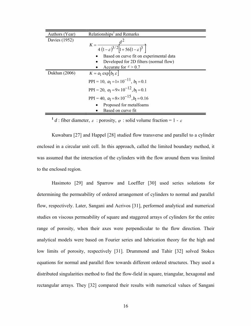
Authors (Year) Relationships1 and RemarksDavies (1952)
32/3
2
156114
dK
Based on curve fit on experimental data Developed for 2D filters (normal flow) Accurate for > 0.7
Dukhan (2006) 11 exp baK
PPI = 10, 1.0,101 111
1 ba
PPI = 20, 1.0,109 112
1 ba
PPI = 40, 16.0,108 115
1 ba
Proposed for metalfoams Based on curve fit
1 d : fiber diameter, : porosity, : solid volume fraction = 1 -
Kuwabara [27] and Happel [28] studied flow transverse and parallel to a cylinder
enclosed in a circular unit cell. In this approach, called the limited boundary method, it
was assumed that the interaction of the cylinders with the flow around them was limited
to the enclosed region.
Hasimoto [29] and Sparrow and Loeffler [30] used series solutions for
determining the permeability of ordered arrangement of cylinders to normal and parallel
flow, respectively. Later, Sangani and Acrivos [31], performed analytical and numerical
studies on viscous permeability of square and staggered arrays of cylinders for the entire
range of porosity, when their axes were perpendicular to the flow direction. Their
analytical models were based on Fourier series and lubrication theory for the high and
low limits of porosity, respectively [31]. Drummond and Tahir [32] solved Stokes
equations for normal and parallel flow towards different ordered structures. They used a
distributed singularities method to find the flow-field in square, triangular, hexagonal and
rectangular arrays. They [32] compared their results with numerical values of Sangani

17
and Acrivos [31] for normal flow and Happel [28] for the parallel case. The model of
Drummond and Tahir [32] for normal permeability was very close to the analytical model
of Sangani and Acrivos [31]; thus, it is only accurate for highly porous materials where
> 0.7.
Keller [33] and Gebart [34] assumed that the permeability of ordered fibrous
structures is controlled by the narrow slots formed between the fibers; they applied the
lubrication theory to determine the flow resistance through the gap. It should be noted
that the lubrication theory is usually valid in the limit of close-packed fibers, < 0.65.
The abovementioned models are compared with experimental data in Section 2.4.
The numerical studies on the flow through fibrous media are summarized in Table
2. Several researchers have numerically simulated the creeping flow through ordered
cylinders [31, 35-38]. In general, numerical simulations cover a wider range of porosity
and fiber distribution in applying the unit cell approach for 1D, 2D, and 3D structures.
Sangani and Yao [39] extended the studies of Sangani and Acrivos [31] for ordered
structures to 1D cylinders in random distribution. Higdon and Ford [40] used a spectral
boundary element formulation to calculate the hydraulic permeability of ordered,
monomodal, three dimensional fibrous media. They considered simple cubic (SC), body-
centered cubic (BCC), and face-centered cubic (FCC) arrangements of fibers in a unit
cell. Applying a singularity method, Clague and Philips [41] computed the permeability
of ordered periodic arrays of cylinders and of disordered cubic (periodic) cells of
cylindrical fibers. Clague et al. [42] employed a lattice-Boltzmann technique to study
similar geometries and extended their studies to include bounded structures. Sobera and
Kleijn [37] studied the permeability of 1D and 2D ordered and random fibrous media

18
both analytically and numerically. Their analytical model was a modification of the scale
analysis proposed by Clauge et al. [42]. Boomsma et al. [43] used a finite volume method
to solve the flow inside dodecahedral and tetrahedral unit cells to investigate flow
properties of metalfoams. Palassini and Remuzzi [44] employed a finite element method
to solve the Stokes equation for a tetrahedral array of fibers to predict the flow properties
of glomerular basement membrane.
Random microstructure approach: As a result of the recent significant growth
of computational power, several researchers have tried to perform simulations on
microstructures formed by a higher number of cylindrical fibers. These researchers have
generated random microstructures that resemble the actual fibrous materials for different
applications.
Clauge and Philips [41] were among the pioneers in employing random
microstructure approach. They used a numerical version of slender body theory to
determine permeability of monodisperse and polydisperse random fibrous
microstructures. Stylianopolous et al. [45], Clauge et al. [42], and Tahir and Tafreshi
[46], used finite element, lattice Boltzmann, and finite volume methods, respectively to
solve creeping flow inside 3D random fibrous structures. Koponen et al. [47] and Zobel
et al. [48] performed numerical simulations for 2D structures using lattice Boltzmann and
finite elements methods, respectively.
Hao and Cheng [49] solved creeping flow through a mesh of 2D random fibers
over a wide range of porosity > 0.6 to model the GDL of PEM fuel cells. They used a
Lattice Boltzmann method in their study. In a similar study Nabovati et al. [50]

19
performed lattice Boltzmann simulations for 3D random structures in the porosity range
of > 0.15. They also reported a correlation for calculating permeability. Lattice
Boltzmann simulations of gas flow through several random fibrous structures were
carried out by Vandoormaal and Pharoah [51] over the porosity range of 0.6 < < 0.8.
They reported numerical results for different fiber orientations which were an order of
magnitude different in a constant porosity.
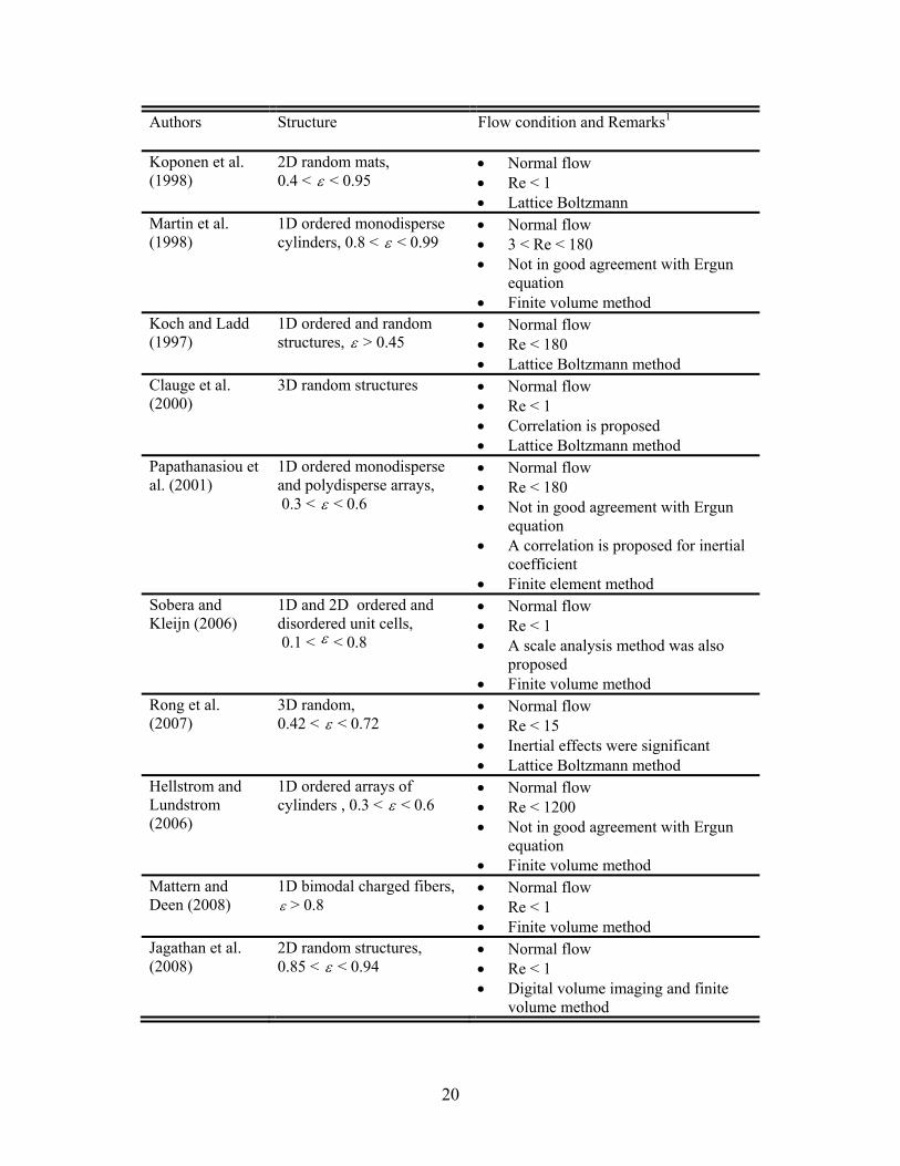
Table 2: Summary of the selected numerical studies for fibrous media.
Authors Structure Flow condition and Remarks1
Sangani and Yao (1988)
1D ordered and random arrays of monodisperse cylinders, 0.3 < < 0.9
Normal and parallel flow Re < 1 Multipole expansion method
Sahraoui and Kaviany (1992)
1D ordered and deformed cylinders, 0.4 < < 0.8
Normal flow Re < 200 Good agreement with
experimental data Finite volume method
Edwards et al. (1990)
1D ordered monodisperse and polydisperse cylinders, 0.4 < < 0.8
Normal flow Re < 180 Not in good agreement with
Ergun equation Finite element method
Higdon and Ford (1996)
1D and 3D ordered unit cells, the entire range of porosity
Normal flow Re < 180 Boundary element method
Ghaddar (1995) 1D ordered and random, 0.4 < < 0.8
Normal flow Re < 200 In good agreement with experimental
data Parallel finite element method
Johson and Deen (1996)
2D unit cell, = 0.32 Normal flow Re < 1 Finite element method
Clauge and Philips (1997)
3D random monodisperse and polydisperse structures
Normal flow Re < 1 Slender body theory
20
Authors Structure Flow condition and Remarks1
Koponen et al. (1998)
2D random mats, 0.4 < < 0.95
Normal flow Re < 1 Lattice Boltzmann
Martin et al. (1998)
1D ordered monodisperse cylinders, 0.8 < < 0.99
Normal flow 3 < Re < 180 Not in good agreement with Ergun
equation Finite volume method
Koch and Ladd (1997)
1D ordered and random structures, > 0.45
Normal flow Re < 180 Lattice Boltzmann method
Clauge et al. (2000)
3D random structures Normal flow Re < 1 Correlation is proposed Lattice Boltzmann method
Papathanasiou et al. (2001)
1D ordered monodisperse and polydisperse arrays, 0.3 < < 0.6
Normal flow Re < 180 Not in good agreement with Ergun
equation A correlation is proposed for inertial
coefficient Finite element method
Sobera and Kleijn (2006)
1D and 2D ordered and disordered unit cells, 0.1 < < 0.8
Normal flow Re < 1 A scale analysis method was also
proposed Finite volume method
Rong et al. (2007)
3D random, 0.42 < < 0.72
Normal flow Re < 15 Inertial effects were significant Lattice Boltzmann method
Hellstrom and Lundstrom (2006)
1D ordered arrays of cylinders , 0.3 < < 0.6
Normal flow Re < 1200 Not in good agreement with Ergun
equation Finite volume method
Mattern and Deen (2008)
1D bimodal charged fibers, > 0.8
Normal flow Re < 1 Finite volume method
Jagathan et al. (2008)
2D random structures, 0.85 < < 0.94
Normal flow Re < 1 Digital volume imaging and finite
volume method
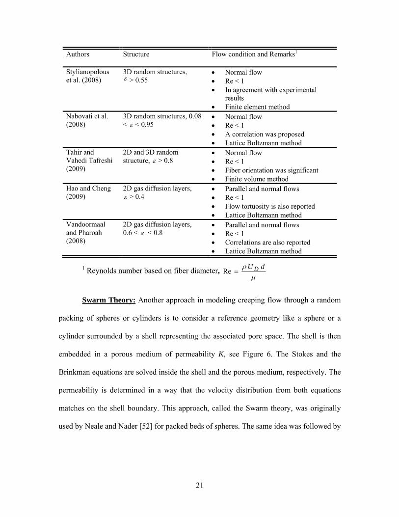
21
Authors Structure Flow condition and Remarks1
Stylianopolous et al. (2008)
3D random structures, > 0.55
Normal flow Re < 1 In agreement with experimental
results Finite element method
Nabovati et al. (2008)
3D random structures, 0.08 < < 0.95
Normal flow Re < 1 A correlation was proposed Lattice Boltzmann method
Tahir and Vahedi Tafreshi (2009)
2D and 3D random structure, > 0.8
Normal flow Re < 1 Fiber orientation was significant Finite volume method
Hao and Cheng (2009)
2D gas diffusion layers, > 0.4
Parallel and normal flows Re < 1 Flow tortuosity is also reported Lattice Boltzmann method
Vandoormaal and Pharoah (2008)
2D gas diffusion layers, 0.6 < < 0.8
Parallel and normal flows Re < 1 Correlations are also reported Lattice Boltzmann method
1 Reynolds number based on fiber diameter,
dU DRe
Swarm Theory: Another approach in modeling creeping flow through a random
packing of spheres or cylinders is to consider a reference geometry like a sphere or a
cylinder surrounded by a shell representing the associated pore space. The shell is then
embedded in a porous medium of permeability K, see Figure 6. The Stokes and the
Brinkman equations are solved inside the shell and the porous medium, respectively. The
permeability is determined in a way that the velocity distribution from both equations
matches on the shell boundary. This approach, called the Swarm theory, was originally
used by Neale and Nader [52] for packed beds of spheres. The same idea was followed by

22
Spielman and Goran [5] for 2D and 3D fibrous structures. They proposed two implicit
models for calculating the permeability of such structures which are presented in Table 1.
2.1.3 Blending rules (Mixing rules)
An approximate method that has been used by researchers to estimate the
permeability of real fibrous media is the blending technique. In this approach, the
complex porous microstructure is modeled as a mixture/combination of fibrous structures
with known permeability [53]. As such, it is expected that the equivalent permeability,
eqK , to be related to the permeability of each component; the concept of blending
technique for 2D fibrous mats is shown in Figure 7. It should be noted that there is no
concrete rule for estimating the mixtures’ permeability. This approach was originally
proposed by Happel [28] for predicting the permeability of 3D random materials which
was not successful. In more recent studies, blending techniques have been successfully
employed to estimate the permeability of fibrous mixtures such as hydrogels [54], fibers
with different sizes [41], and fibers with different charges [55, 56].
Figure 6: Schematic of the swarm theory approach.
r = a
r = b
UD

23
Flow
Parallel to flow
direction
Normal to flow
direction
2D structure
Figure 7: The blending technique concept for 2D structures.
2.1.4 Analogy of hydraulic permeability with other diffusive properties
Several researchers have tried to relate the permeability to different measurable
transport properties of the porous medium. One of the properties that has been used for
calculating the permeability is the electrical formation factor, F, which is defined as [20]:
eF
1
(9)
where e is the effective electrical conductivity of a porous medium of an insulating
solid containing a conducting fluid of conductivity 1 .
Johnson et al. [57] proposed the following approximate relation involving the
electrical conductivity:

24
FK
8
2
(10)
where:
dsrE
dVrE2
2
)(
)(
2 (11)
E(r) is the local electric-field, dV and dS denote integrations over volume and the pore-
solid surface, respectively. The parameter is a weighted pore volume-to-surface ratio
that provides a measure of the dynamically connected parts of the pore region.
Tomadakis and Sotirchos [58] used a random-walk simulation method to calculate the
formation factor for randomly distributed overlapping fibers. Using their simulations
results and combining Eqs. (10) and (11), Tomadakis and Robertson [11] reported a
model for calculating permeability of 1D, 2D, and 3D fibrous structures, see Table 1.
2.1.5 Experimental studies
As a result of the diverse applications of fibrous materials, numerous
experimental studies have been conducted for determination of the permeability of
fibrous media; see for example [22, 36, 48, 59-71]. Good reviews of experimental works
are available in Jackson and James [54], Astrom et al. [15], and Tomadakis and
Robertson [11]. Although our motivation for the present study is mostly coming from
sustainable energy applications such as fuel cell technology and use of metalfoams as
media for heat transfer, a selection of experimental studies on various fibrous materials is
summarized in Table 3. The experimental studies are selected such that structure
inhomogeneity, channeling, fiber mobility, deflection, compression, fiber bending, fiber

25
surface slip, non-viscous flow, inertial effects, tube wall friction, capillary effects, surface
tension, gas compressibility, fiber shape/size distribution, and fiber aspect ratio effects
were not involved in the measurements.
There are few experimental studies available in the literature that reported the
permeability of GDLs in creeping flow regime. Williams et al. [72], Ihonen et al. [73],
and Mueller et al. [74] measured the through-plane permeability of several GDLs. Most
of their measurements were affected by existence of the micro porous layer. Prasanna et
al. [75] and Mathias et al. [76] reported the through-plane permeability of several bare
GDLs with various PTFE loadings.
Ihonen et al. [73] showed that a reverse relationship exists between the in-plane
permeability and compression. Recently, Feser et al. [8] studied the effects of
compression and reported in-plane gas permeability as a function of porosity for a carbon
cloth, a non-woven carbon fiber GDL, and a carbon paper. In a similar work, Gostick et
al. [9] measured permeability of several commercial GDLs under various compressive
loads and reported the in-plane permeability as a function of porosity. They also reported
the through plane permeability of these GDLs. More details of the experimental studies
can be found in Ref. [77].
2.2 Inertial flow regime (moderate Reynolds numbers)
Including the inertial effects in the flow analysis adds to the complexity of the
problem. As such, the moderate Reynolds number flows through fibrous structures are
mostly studied either numerically or experimentally rather than analytically in the
literature.

26
2.2.1 Theoretical studies
Khan et al. [78] employed an integral technique solution to determine pressure
drop in tube banks with regular cylinder arrays, analytically. The velocity profiles were
calculated from a combination of the potential flow and the boundary layer theories.
Their model was developed for high Reynolds number flows, Re > 100, and could
capture trends of the experimental data reported by others qualitatively.
Effects of Reynolds number on the pressure drop through unidirectional mono-
disperse and bimodal fibers were investigated numerically by Nagelhout et al. [79],
Martin et al. [80], Lee and Yang [81], Koch and Lodd [82], Edwards et al. [83], Ghaddar
[84], and Papathanasiou et al. [85]. Their results, in general, confirmed the existence of a
parabolic relationship between pressure drop and flow rate in the considered geometries.
However, comparison of these numerical results with conventional models in the
literature such as the Ergun equation was not successful [85].
The studies of moderate Reynolds number flows through 2D and 3D structures
are not frequent. Recently, Rong et al. [86] used Lattice Boltzmann method to investigate
flow in three dimensional random fiber network with porosities in the range of 0.48 <
< 0.72. Their results were in agreement with Forchheimer equation which is in line with
the observations of [86]. Boomsma et al. [43] have also studied flow in high porosity 3D
fibrous structures to predict the flow properties of open cell aluminum foams.

27
Table 3: Summary of the selected experimental studies for flow properties of fibrous media.
Authors Material Fiber category (flow direction)
Test fluid
maxRe
Fiber diameter (mm)
Carman (1938) stainless steel wire, 0.681 < < 0.765 Random 3D (normal)
Glycerol 0.5
0.328
Wiggins et al. (1939)
Glass rods, copper wire, glass wool, and fiber glass, 0.685 < <0. 93 Random 3D (normal)
Water 8
0.007-0.408
Sullivan (1942)
Drill rod, copper wire, goat wool, Chinese hair, and blond hair Ordered and random 1D (parallel)
Air N.A.
0.008-7.2
Bergelin et al. (1950)
Various arrangements of tubes, 0.42 < < 0.65 Ordered 1D (normal)
Silicon oil 10
9.52, 19.04
Davies (1952) Glass wool, kapok, rayon, > 0.8 Random 2D (normal and parallel)
Air N.A.
N.A.
Kirsch and Fuchs (1967)
Various arrangements of kapron tubes, > 0.7 Ordered 1D (normal)
Water 0.005
0.15, 0.225, 0.4
Kostornov and Schevchuck (1977)
Kapron fibers 2D random (normal)
Water, alcohol 10
N.A.
Jackson and James (1982)
Hyaluronic acid polymer, > 0.99 3D random (normal)
Water 1×10-11
1×10⁻⁶
Gutowski et al. (1987)
Fiber mats 0.2 < < 0.5 1D random (normal)
Silicon oil N.A..
0.008
Skartsis et al. (1992)
Random carbon fibers and ordered aluminum rods, 0.4 < < 0.7 1D ordered and random (normal and parallel)
Water, Silicon oil N.A..
1.19-1.59
Chmielewski and Jayaraman (1992)
Acrylic rods in ordered arrangement, = 0.7 1D ordered (normal)
Polybutene H25 and kerosene 0.3
4.76
Khomami and Moreno (1997)
Acrylic rods, 0.45 < < 0.85 1D ordered (normal)
Silicon oil N.A.
7.1, 14.2
Rahli et al. (1997) Bronze and copper rods, 0.4 < < 0.9 3D random (normal)
Water N.A.
0.15

28
Authors Material Fiber category (flow direction)
Test fluid
maxRe
Fiber diameter (mm)
Shih and Lee (1998)
Random fiber mat U750, 0.4 < < 0.7 2D random (parallel)
Diphenyl-octyl-pthalate N.A.
0.02
Zhong et al. (2006)
Acrylic rods, 0.9 < < 0.975 1D ordered (normal)
Glycerol-water mixture 0.17
3.18
Zobel et al. (2007) Polypropylene fibers, 0.7 < < 0.9 2D random (normal)
Air N.A.
0.015
Williams et al. (2004)
Gas diffusion layer 2D random (normal)
Air N.A.
0.007-0.001
Ihonen et al. (2004)
Gas diffusion layer 2D random (normal and parallel)
Air N.A.
0.009
Prasanna et al. (2004)
Gas Diffusion layer, < 0.78 2D random (normal)
Air N.A.
0.009
Feser et al. (2006) Gas Diffusion layer, 0.7 < < 0.78 2D random (parallel)
Air N.A.
0.009
Gostick et al. (2006)
Gas Diffusion layer, 0.65 < < 0.85 2D random (normal and parallel)
Air N.A.
0.007-0.001
Hunt and Tien (1988)
Chrome, aluminum, and nickel foams, 0.94 < < 0.97 3D random (normal)
Water ReK = 100 1
N.A.
Calmidi and Mahajan (2000)
Aluminum foam, 0.9 < < 0.97 3D random (normal)
Air ReK = 135
0.25-0.5
Boomsma and Poulikakos (2002)
Compressed aluminum foam, 0.61 < < 0.93 3D random (normal)
Air ReK = 27
N.A.
Hwang et al. (2002)
Aluminum foam, 0.7 < < 0.9 3D random (normal)
Air Rep = 7800 2
N.A.
Bhattacharya et al. (2002)
Aluminum foam, 0.9 < < 0.98 3D random (normal)
Air N.A.
0.2-0.55
Boomsma et al. (2003)
Comressed aluminum foam, 0.61 < < 0.93 3D random (normal)
Air ReK = 140
N.A.
Kim et al. (2003) Aluminum foam, = 0.92 3D random (normal)
Air Rep = 2900
0.2-0.4

29
Authors Material Fiber category (flow direction)
Test fluid
maxRe
Fiber diameter (mm)
Khayargoli et al. (2004)
Nickel and nickel-chromium, 0.83 < < 0.9 3D random (normal)
Air N.A.
N.A.
Tadrist et al. (2004)
Comressed aluminum foam, 0.88 < < 0.89 3D random (normal)
Air N.A.
0.69-1
Dukhan (2006) Comressed aluminum foam, 0.68 < < 0.92 3D random (normal)
Air Rep = 1000
0.25-0.5
Bonnet et al. (2008)
Copper, nickel, and nickel-chromium 3D random (normal)
Air, water Rep = 2000
N.A.
1 ReK : Reynolds number based on K ,
KU DRe
2 Rep : Reynolds number based on pore diameter, pD dU
Re
2.2.2 Experimental studies (moderate Reynolds numbers)
Most of the high Reynolds number (Re > 1000) experimental studies on porous
media have been done to investigate the flow properties of heat exchangers. As a result,
accurate correlations have been presented for the turbulent flow properties of 1D tube
banks; see for example [87]. Recently, metalfoams have received an especial attention
because of their thermophyscial properties that make them good candidates for compact
heat exchangers. In metalfoams, the flow Reynolds numbers based on fiber diameter
typically range from 10 to 500. In this range, the pressure drop is related to volume-
averaged velocity through the Forchheimer equation, Eq. (2) and both terms have the
same order of magnitude in the overall pressure drop.
Bergelin et al. [88] measured the pressure drop across several tube bank arrays for
Re < 1000. Kirsch and Fuchs [63] studied similar structures for Re < 10 and found out
30
that the onset of transition from the Darcy equation to the Forchheimer equation is Re
5-8. Few other studies have been conducted for moderate Reynolds flow through fibrous
materials which are listed in.
Hunt and Tien [89] were among the pioneers to investigate thermophysical
properties of metalfoams in 1980s. Since then, several experimental works have reported
the permeability and the inertial coefficient of various metalfoams [2, 90-100]; these
studies are summarized in Table 3. It should be noted that the minimum Reynolds
number in the listed studies generally has been higher than 1; this can affect the accuracy
of the reported values for the permeability.
2.3 Flow through channels partially-/fully-filled with porous media
Although the fully-developed and developing flows in channels of various cross-
sections filled with porous media have been extensively studied in the literature, see for
example [101-103]; however, such studies for micron size channels are not numerous.
Hooman and his coworkers [104, 105] have investigated rarefied gas flows in
microchannels filled with porous media. But, their theoretical analyses were not verified
by experimental data. Few experimental studies have been conducted to study the flow
through mini/microchannels filled with micro pin fins. Kosar et al. [106] studied laminar
flow across four different arrays of micro pin fins embedded inside microchannels with
100 m depth. The pin fin diameters in their study were 50 and 100 m . They compared
their results for Reynolds numbers in the range of 5-128 with existing correlations for
relatively high Reynolds number flows through macro-scale tube banks and observed a
significant deviation. Kosar et al. [106] related this deviation to the difference(s) between
31
flow in micron and regular-size systems. Vanapalli et al. [107] measured the pressure
drop in microchannels of 250 m depth containing various pillar arrays in the Reynolds
number range of 50-500. On the contrary, their results for circular pillars were in good
agreement with conventional relationships. Yeom et al. [108] reported low Reynolds
number flow pressure drops through micro-porous channels with various fibers in square
arrangements. The channels were 200 m deep and the diameters of the microposts
ranged from 200 m to less than 10 m . Similar to [107], Yeom et al. [108] did not
include wall effects into their analysis. Therefore, their results for high permeability
arrays deviated from the values predicted by conventional theories.
Fluid flow in channels or systems partially filled with porous media has a wide
range of engineering applications such as electronic cooling, transpiration cooling, drying
processes, thermal insulation, oil extraction, and geothermal engineering. The two main
challenges involved in modeling this problem are: i) estimating the flow properties of
porous media and ii) finding accurate boundary conditions for the interface region.
Beaver and Joseph [109] were among the pioneers that investigated the interface
boundary condition. They noticed a slip in the experimental values of velocity at the
interface region. Vafai and Kim [110] developed an analytical solution for fluid flow at
the interface between a saturated porous medium and a fluid layer. Kuznetsov [111]
extended the analysis of [110] to higher Reynolds number flows and included the inertial
effects in his analytical solution. Velocity distribution for channels partially filled with
cylinders aligned with the flow direction was reported by Davis and James [112].
Velocity distribution in channels partially filled porous media has been studied

32
experimentally more recently by Tachie et al. [113], Agelinchaab et al. [114], and Arthur
et al. [115] for porous media comprised of regular arrays of cylinders.
To capture the interface velocity distribution more accurately, sophisticated
boundary conditions has been proposed by Ochoa-Tapia and Whitaker [116] and
Sahraoui and Kaviany [38]. However, numerical simulations of Alazmi and Vafai [117]
showed that the difference in the predicted velocity distributions using various boundary
conditions was not significant.
2.4 Comparison of the existing models with experimental data
The existing models/correlations for permeability of 1D, 2D, 3D, and metalfoams,
listed in Table 1, are compared with the experimental data collected from various sources.
Based on Figure 8-Figure 12 and the literature review in Sections 2.1-2.3 the following
conclusions can be made:
The existing models for 1D, 2D, and 3D fibrous structures have limited ranges of
accuracy and none of them can cover the entire range of porosity.
Most of the existing models can only capture the trends of experimental data
qualitatively.
The effects of microstructure and geometrical parameters including fiber
orientation and enclosing walls on flow properties of fibrous materials are not
included in the majority of existing models.
No analytical model exists for the permeability of gas diffusion layer of fuel cells.

33
The existing models are incapable of predicting the experimental data for
permeability of fibrous materials with complex microstructure such as
metalfoams.
Effects of GDL compression on the through-plane permeability have not been
investigated.
Experimental data for permeability of metalfoams are usually based on the
measurements in high Reynolds number flow, Re > 1; thus, a lack of such
experiments exists in the creeping flow regime.
Accuracy of conventional theories developed for macro-scale confined porous
media is not verified for microsystems. Moreover, the wall effects are not
studied in micro-porous channels.
Effects of geometrical and structural properties on the pressure drop inside
channels partially filled with porous media are not investigated.
Microscopic velocity distribution, which is required for heat and mass transfer
analyses in fibrous media, is not available even for ordered arrays of cylinder.
In general, one can say that the exiting studies have provided useful insights, but
remained limited to specific ranges of porosity, structure, and size scale. This clearly
indicates the need for a fundamental study and mechanistic models that can accurately
predict the mechanical properties such as permeability and tortuosity as a function of the
microstructural properties.

34
+
+
+
K/d
2
0.4 0.6 0.8 110-4
10-3
10-2
10-1
100
101
102
Berglin et al. (1950)Kirsch and Fuchs (1967)Sadiq et al. (1995)Khomami and Moreno (1997)Zhong et al. (2006)Happel (1959)Sahraoui and Kaviani (1992)Van der Westhuizen (1996)Drummond and Tahir (1984)Gebart (1992)
+
Transverse flow1D square arrays
Figure 8: Comparison of the existing models for transverse (normal) flow permeability of square arrangements with experimental data.
--
--
++
+++
++
+++
K/d
2
0.6 0.75 0.9
10-3
10-2
10-1
100
101
102Davies (1952)Molnar et al. (1989)Kostornov and Shevchuk (1977)Gostick et al. (2006)Zobel et al. (2007)VanDoormaal and Pharoah (2008)Tomadakis and Sotirchos (1993)
-
+
Transverse flow2D structures
Figure 9: Comparison of the existing models for through-plane flow through two directional (2D) structures with experimental data.

35
+ + + + +++
++
K/d
2
0.5 0.6 0.7 0.8 0.910-3
10-2
10-1
100
101 Shi and Lee (1998)Gostick et al. (2006), SGL 10BAGostick et aL. (2006), SGL 24BAGostick et al. (2006), SGL 34BAGostick et al. (2006), TGP 90Feser et al. (2006), TGP 60Tomadakis and Sotirchos (1993)Van Doormal and Pharoah (2009)
+
In-plane flow
2D strucutres
Figure 10: Comparison of the existing models for in-plane flow through two directional (2D) structures with experimental data.
++ +++
+++
+++
+++
++ +++ +++
K/d
2
0.4 0.6 0.8 1
10-2
10-1
100
101
102
103
Jackson and James (1982)
Carman (1938)
Rahli (1997)
Bhattacharya et al. (2002)
Higdon and Ford (1996)
Jackson and James (1986)
Tomadakis and Sotirchos (1993)
+
Transverse flow3D structures
Figure 11: Comparison of the existing models for three directional (3D) structures with experimental data.

36
(a)
K(m
2)
0.9 0.95
10-8
10-7
10-6
Bhattacharya et al. (2002)Calmidi and Mahajan (2000)Bonnet et al. (2008)Dukhan (2006), correlation PPI = 10Dukhan (2006), correlation PPI = 20Dukhan (2006), correlation PPI = 40
Metal foams
(b)
+
+
++
+
++
dp (m)
K(m
2)
0.001 0.002 0.003 0.004 0.005
10-8
10-7
10-6
Bhattacharya et al. (2002)Khayaroli et al. (2004)Tadrist et al. (2004)Bonnet et al. (2008)Boosma and Poulikakos (2002)Calimdi and Mahajan (2000)Bonnet et al. (2008), correlation
+
Metal foams
Figure 12: Comparison of the existing models for metalfoams a) Dukhan [98] and b) Bonnet at al. [97] with experimental data.

37
2.5 Modeling road map
Our critical review of the pertinent literature indicates the need for model(s) that
can predict the permeability and inertial coefficient of fibrous porous materials. The main
objectives of the current work are to:
Develop comprehensive analytical model(s) that can predict the flow
properties of fibrous materials.
Investigate effects of the major relevant geometrical parameters such as
porosity, pore diameter, fiber diameter, and fiber orientation on the flow
properties of fibrous materials.
Study the boundary effects on the macroscopic flow-field and the resulting
pressure drop in confined porous media.
Design and conduct an experimental program, using various fluids, to
verify our theoretical investigation for permeability, inertial coefficient,
and wall (boundary) effects.
The focus of the proposed study will be on developing and verifying general
model(s) that predict the flow properties of fibrous porous media. Following other
analytical studies, a basic cell approach will be used. Based on the microstructure and
flow characteristics, various exact and approximate analytical techniques described in
previous sections will be employed to predict pressure drop and permeability. The
modeling road map in the present study is shown in Figure 13.

38
The developed models and the analytical solutions will be verified through
comparison with numerical simulations and experimental measurements. Due to the
diversity of the investigated problems, three test rigs have been designed to conduct
experiments with different fluids, fibrous material types and sizes, and materials scales.
Figure 13: The modeling road map of the present dissertation.

39
3: FLOW PROPERTIES OF FIBROUS STRUCTURES (MICROSCOPIC ANALYSES)
The modeling road map, shown in Figure 13, has been followed. This chapter
discusses the flow properties of fibrous porous media that can be evaluated through
microscopic analysis of the media.
The simplest representations of fibrous porous media are regular ordered arrays of
cylinders. First, compact models will be developed to predict the permeability of such
structures in different directions. The analysis, then, will be extended to predict the
permeability of more complex microstructures such as 2D and 3D fibrous matrices using
various techniques such mixing rules and scale analysis. To cover a wider range of
Reynolds numbers, numerical simulations are carried out to calculate the inertial
coefficient in various ordered structures.
3.1 Permeability of 1D touching fibers
Since flow cannot pass perpendicular to touching fibers (see figures in Table 4),
the normal permeability of these geometries is zero. Fluid passing parallel to the axis of
unidirectional fibers experiences a channel-like flow; thus, the media is treated as a
combination of parallel constant cross-sectional conduits. Therefore, the permeability can
be related to the pressure drop in these channel-like conduits. In this approach, the cross
sectional area and the perimeter of the channel are required. Pressure drop can be
calculated using Darcy-Weisbach relation [118]:
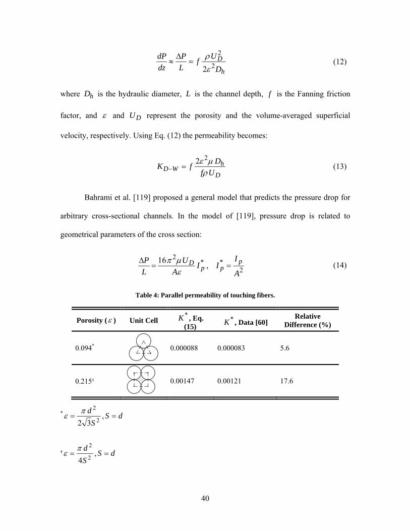
40
h
D
D
Uf
L
P
dz
dP2
2
2
(12)
where hD is the hydraulic diameter, L is the channel depth, f is the Fanning friction
factor, and and DU represent the porosity and the volume-averaged superficial
velocity, respectively. Using Eq. (12) the permeability becomes:
D
hWD Uf
DfK
22
(13)
Bahrami et al. [119] proposed a general model that predicts the pressure drop for
arbitrary cross-sectional channels. In the model of [119], pressure drop is related to
geometrical parameters of the cross section:
2**
2,
16
A
III
A
U
L
P ppp
D
(14)
Table 4: Parallel permeability of touching fibers.
Porosity ( ) Unit Cell *K , Eq. (15)
*K , Data [60] Relative
Difference (%)
0.094*
0.000088 0.000083 5.6
0.215†
0.00147 0.00121 17.6
* dSS
d ,
32 2
2
† dSS
d ,
4 2
2

41
where pI , A , are the polar moment of inertia, the area of the passage cross-section,
and the porosity, respectively. Using the Darcy’s relationship and the model of [119], the
non-dimensional permeability of periodic touching fibrous media can be found as:
*22*
16 pI
A
d
KK
(15)
This relationship can be easily applied to any touching fibrous arrangements including;
triangular, rectangular, hexagonal, and checker boarding.
In Table 4, the values calculated form Eq. (15) are compared with the
experimental data reported by Sullivan [60] for air flowing through staggered and square
arrangements of copper wires, respectively. The difference between the predicted values
by the proposed model and the experimental data is reasonable within the context of
porous media. Equation (15) is also applicable to any foam like materials.
3.2 Determination of the normal permeability of square fiber
arrangements (integral technique)
A powerful method for analyzing fluid mechanic problems without knowing the
exact velocity distribution, is the integral technique solution. In this approach, a general
shape of the velocity profile that satisfies conservation of mass and momentum on the
boundaries is assumed. Then, using the assumed velocity distribution the flow equation is
integrated over the entire region and the resulting pressure drop is determined.

42
Figure 14: Rectangular arrangement of cylinders and the considered unit cell.
For the square arrangement of fibers shown in Figure 14, the unit cell (the
smallest region which has identical flow properties to the whole media) is selected as the
space between parallel cylinders. The porosity for this arrangement is:
2
2
41
S
d
(16)
The permeability is related to the total pressure drop through the unit cell; see Eq.
(1). Employing lubrication theory and neglecting inertial terms, the x -momentum
equation reduces to Stokes equation:
dx
dP
y
u
1
2
2
(17)
Determination of the exact velocity profile requires detail knowledge of the
geometry of the medium which is not feasible in the case of porous media. Moreover,
even with specified geometry and boundary conditions, finding exact analytical solution

43
is not guaranteed and is a difficult task for most cases. To overcome this problem, an
integral method is employed in this study. The integral method provides a powerful
technique for obtaining accurate but approximate solutions to rather complex problems
with remarkable ease. The basic idea is that we assume a general shape of the velocity
profile. It must be noted that we are not interested in the precise shape of velocity profile
but rather need to know the pressure drop over the basic cell to calculate permeability.
This can be accomplished by satisfying conservation of mass and momentum in a lumped
fashion across the unit cell. As a result, an approximate parabolic velocity profile is
considered which satisfies the boundary conditions within the unit cell. The border
velocity is zero on the edge of the cylinders (no-slip condition) and reaches its maximum
value at the half distance between cylinders in the x -direction, see Figure 14. It is also
assumed that the maximum border velocity is a function of the porosity [71], i.e., as the
porosity increases the maximum border velocity increases accordingly. For lower
porosities, the border velocity is very small and for highly porous limits, it approaches to
the Darcy velocity. In this study, the border velocity increases linearly from the edge of
the fibers ( bu = 0) to its peak at the center of the unit cell:
274.0274.1)(22
,2
)(
g
Sx
d
dS
xgUu Db
(18)
Moreover, the maximum border velocity is related to porosity through g( )
where g(0.215) =0 for touching fibers and g(1) =1 for high porosity limits. Therefore, the
following velocity distribution is considered:

44
22,
2)(
4
20,
42
2
1
22
2
2
22
Sx
dU
dS
xgy
S
dxyx
dS
dx
dPu
D
(19)
The total pressure drop of the unit cell is calculated employing an integral
technique solution. In this approach, using continuity equation and the definition of
volumetric flow rate, one can calculate pressure gradient as:
20,
42
3
322
dx
xdS
Q
dx
dp
(20)
22
,2
)(112
3S
xd
dS
xgdS
S
Q
dx
dP
(21)
The pressure drop in the basic cell is calculated as:
2
)(2)(
12
2tan3
)(
26
3
2
522
22
12
22
gdS
S
Q
dS
dS
dSd
SdS
dQP cellunit
(22)
Using the Darcy equation and introducing solid fraction as 1 , the permeability of
square arrangement becomes:

45
1
2
5
1
2*
1
21
1tan18
1
11218
2
)(2112
g
K
(23)
where 2* / dKK , 274.0274.1)( g , and 4/ . In Figure 15, Eq. (23) is
compared with experimental data collected from several sources [61, 63, 68, 71, 120].
The 15% bounds of the model are also shown in the plot, to better demonstrate the
agreement between the data and the model. The experiments were conducted using
different fluids including: air, water, oil, and glycerol with a variety of porous materials
such as metallic rods, glass wool, and carbon. It can be seen that the proposed model, i.e.,
Eq. (23), accurately predicts the trend of experimental data for square arrangement of
fibers over the entire range of porosity [121].
To further investigate the accuracy of the assumed velocity distribution, creeping flow
through the unit cell shown in Figure 14 was solved numerically using Fluent software
[122]. Structured numerical grids with aspect ratios in the range of 1-5 were generated
using Gambit [122]. SIMPLE algorithm was employed for pressure-velocity coupling
[123].
Although fully-developed solution for normal flow can be found by simulating a single
basic cell and applying periodic boundary condition to determine the developing length
for flow in the medium, a set of 7-10 unit cells in series are considered and velocity
profiles are compared at the entrance to each unit cell; details of the numerical results are
provided in Appendix C. The inlet velocity of the media was assumed to be uniform.
Constant pressure boundary condition was applied on the computational domain outlet.
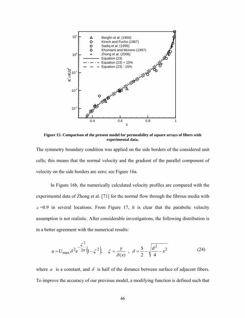
46
+
+
+
K* =
K/d
2
0.4 0.6 0.8 1
10-3
10-2
10-1
100
101Berglin et al. (1950)Kirsch and Fuchs (1967)Sadiq et al. (1995)Khomami and Moreno (1997)Zhong et al. (2006)Equation (23)Equation (23) + 15%Equation (23) - 15%
+
Figure 15: Comparison of the present model for permeability of square arrays of fibers with experimental data.
The symmetry boundary condition was applied on the side borders of the considered unit
cells; this means that the normal velocity and the gradient of the parallel component of
velocity on the side borders are zero; see Figure 16a.
In Figure 16b, the numerically calculated velocity profiles are compared with the
experimental data of Zhong et al. [71] for the normal flow through the fibrous media with
=0.9 in several locations. From Figure 17, it is clear that the parabolic velocity
assumption is not realistic. After considerable investigations, the following distribution is
in a better agreement with the numerical results:
22
222max 42
,)(
,1
2
xdS
x
yeUu
(24)
where is a constant, and is half of the distance between surface of adjacent fibers.
To improve the accuracy of our previous model, a modifying function is defined such that

47
compensates for the difference between the numerical values of pressure drop and those
obtained from parabolic velocity assumption on the cylinders:
)(fPP parabolic
(25)
(a)
(b)
u/UD
y/S
0.5 1 1.5 20
0.25
0.5
0.75
1
Zhong et al. (2006), x/S=0.0Zhong et al. (2006), x/S=0.28Zhong et al. (2006), x/S=0.5Present study, x/S=0.0Present study, x/S=0.28Present study, x/S=0.5
Figure 16: a) A typical numerical grid and the boundary conditions used in the analysis for = 0.65, b) comparison of the present numerical and the experimental data for the velocity profiles in normal
flow and = 0.9.

48
u/UD
0.5 1 1.5 2
Parabolic profile
Present study
x/S=0.17
y/S
0 1 20
0.2
0.4
0.6
0.8
1
Parabolic profile
Present study
x/S=0.0
0.5 1 1.5
Parabolic profile
Present Study
x/S=0.28
Figure 17: Comparison of the present numerical and parabolic velocity profiles in normal flow, = 0.9.
Several functions were tested and the following correlation was found accurate for
predicting the correction function:
58.2/1341.1343.1)( f
(26)
Therefore, the normal permeability of square arrangement becomes:
)1(4
,4
1341.1343.114
54
1
1121858.2/11
5.22*
K
(27)
This equation can predict the numerical results within 5% accuracy over the entire range
of porosity.
3.3 Parallel permeability of ordered arrangements
In the following sub-sections, parallel flow through various ordered arrangements,
shown in Figure 18, will be investigated [124].

49
Using geometric symmetry, only the selected regions of the unit cells are
considered in the analysis. The solid volume fraction ( ) and porosity ( ) of square,
staggered, and hexagonal arrays are:
Hexagonal33
Staggered32
Square4
1
2
2
2
2
2
2
S
d
S
d
S
d
(28)
Therefore, the minimum possible values of for square, staggered, and hexagonal
arrangements with no overlapping are 0.215, 0.094, and 0.395, respectively. These values
indicate the touching limit of fibers.
The conservation of linear momentum, Poisson’s equation, in the cylindrical
coordinate system reads:
dz
dP
r
w
rr
w
r
w
1
22
2
2
2
(29)
where w is the velocity component in the z-direction. Following Sparrow and Loeffler
[30], the general solution of the Poisson’s equation in the cylindrical coordinate is
considered:
1
2sincos
4ln
kkk
kk
kk kFkErDrC
dz
dPrrBAw
(30)

50
For square arrangement, symmetry lines are located at = 0 and = /4. The
first condition results in kF = 0 and the second condition holds when k = 4, 8, 12, … .
The no-slip boundary condition on the solid walls leads to:
dz
dPrrBAandrCD k
kk 4ln
20
02
0
(31)
Figure 18: Unit cell for a) square, b) staggered, and c) hexagonal arrangements.

51
Total frictional force exerted on the fluid by solid rods must be balanced by the net
pressure force acting over the entire cross-section of the basic cell:
4/
0
cos2/4/
0 00
0
S
rddrr
dz
dPdr
r
w
rr (32)
Solving for Eq. (32), the constant B can be found:
dz
dPSB
2
2
(33)
Consequently, the velocity distribution becomes:
2/
4
4cos24
1ln
2
,
,][
2*
1
44244
242
2
2*
d
r
dz
dPd
ww
kS
dG
d
Sw
k
kkkk
kk
(34)
The last constant, kG , is found by applying the symmetry condition on the unit cell
border where cos2/Sr . Therefore, one can write:
014coscos
14coscos
2
1cos
2
1
8
14
2
k
k
kk k
S
dk
g
(35)
where:
24
24
k
kkS
kGg
(36)

52
Sparrow and Loeffler [30] applied Eq. (35) at a finite number of points along the
boundary and solved the resulting set of linear equations to determine the unknown
coefficients, i.e., kg . The same approach is followed here and the calculated coefficients
for several porosities are listed in Table 5. The listed values are in agreement with the
values reported by Sparrow and Loeffler [30].
The triangular unit cell section for the staggered fiber arrangements is shown in
Figure 18b. The symmetry boundaries are located at = 0 and = /6. The governing
equation and its general solution are still Eqs. (29) and (30). Following the same
procedure described above and applying symmetry boundary conditions, one can find:
][1
66262
2
2* 6cos
64
1ln
3
k
kkk
k kS
d
k
g
d
Sw
(37)
The unknown coefficients are evaluated with the same approach used for square
arrangements and the results as listed in Table 5.
Adopting the same approach and considering the location of the symmetry lines
for hexagonal arrays at = 0 and = /3, the velocity distribution can be found as:
][1
33232
2
2* 3cos
34
1ln
2
33
k
kkk
k kS
d
k
g
d
Sw
(38)
The unknown coefficients are listed in Table 5. From the listed coefficients in
Table 5 and the form of the series solutions in Eqs. (34), (37), and (38), it is expected that
truncating the series from the second term, does not affect the velocity distributions
significantly. Our analysis also showed that substituting 1g with an average value has a

53
negligible impact on the predicted results (less than 4 percent). Therefore, 1g is replaced
by -0.107, -0.0437, and -0.246 for square, staggered, and hexagonal arrangements,
respectively. Hence, the velocity distributions become [124]:
Table 5: Calculated coefficients in velocity distribution.
Square arrangement
dS / 1g 2g 3g 4g 5g
4.0 0.95 -0.1253 -0.0106 -0.0006 0 0
2.0 0.80 -0.1250 -0.0105 -0.0006 0 0
1.5 0.65 -0.1225 -0.0091 -0.0002 0 0
1.2 0.45 -0.1104 -0.0024 -0.0015 0.0003 0
1.1 0.35 -0.0987 0.0036 0.0029 0.0005 0
1.05 0.29 -0.0904 0.0073 0.0032 0.0002 0
Staggered arrangement
dS / 1g 2g 3g 4g 5g
4.0 0.94 -0.0505 -0.0008 0.0000 0 0
2.0 0.77 -0. 0505 -0.0008 0.0000 0 0
1.5 0.60 -0. 0502 -0.0007 0.0001 0 0
1.2 0.37 -0. 0469 0.0007 0.0002 0.0000 0
1.1 0.25 -0.0416 0.0028 0.0004 0.0000 0
1.05 0.18 -0.0368 0.0043 0.0003 -0.0001 0.0000
Hexagonal arrangement
dS / 1g 2g 3g 4g 5g
4.0 0.96 -0.2850 -0.0365 -0.0048 -0.0006 -0.0001
2.0 0.85 -0.2827 -0.0350 -0.0043 -0.0005 0.0000
1.5 0.73 -0.2728 -0.0286 -0.0019 0.0002 0.0001
1.2 0.58 -0.2433 -0.0096 0.0053 0.0021 0.0006
1.1 0.50 -0.2216 0.0038 0.0093 0.0029 0.0004
1.05 0.45 -0.2076 0.0116 0.0103 0.0027 -0.0003

54
Hexagonal3cos082.0
4
1ln
2
33
Staggered6cos007.0
4
1ln
3
Square4cos0287.0
4
1ln
2
332
2
2
664
42
2
2
442
22
2
2
*
S
d
d
S
S
d
d
S
S
d
d
S
w
(39)
3.3.1 Numerical simulations
Due to the lack of experimental and numerical data for parallel flow through
ordered arrangements of fibers [15], a numerical study is performed using Fluent
software [122] to verify the velocity distributions reported in Eq. (39). Structured grids
are generated using Gambit [122], the preprocessor in the Fluent [122] package;
numerical grid aspect ratios are kept in the range of 1-5. Fluent [122] is a finite volume
based code and a second order upwind scheme is selected to discretize the governing
equations. SIMPLE algorithm is employed for pressure-velocity coupling.
The inlet velocity to the media is assumed to be uniform; this assumption allows
one to study the developing length. To ensure that the fully-developed condition is
achieved, as shown in Figure 19, very long cylinders are considered, i.e., L/d > 40; the
fully-developed section pressure drops are used for calculating the permeability. Constant
pressure boundary condition is applied on the computational domain outlet. The
symmetry boundary condition is applied on the side borders of the unit cells. Grid
independence is tested for different cases and the size of computational grids used for
each geometry is selected such that the maximum difference in the predicted values for
pressure gradient is less than 2%. The convergence criterion, i.e., the maximum relative
error in the value of dependent variables between two successive iterations, is set at 10-6.

55
Figure 19: A typical numerical grid used in the numerical analysis a square arrangement with = 0.9.
To verify the proposed velocity distribution for the square arrangements,
numerical and analytical velocity profiles are plotted in Figure 20 and Figure 21 for
square and staggered arrangements. The velocity magnitudes are nondimensionalized
using the volume averaged velocity, DU . These figures indicate that Eq. (39) accurately
predicts the velocity distribution in the considered geometries.
3.3.1 Parallel permeability
Velocity distributions are developed analytically for parallel flow through square,
staggered, and hexagonal arrays of cylinders in previous sections. Moreover, the flow-
fields are solved numerically to verify the theoretical results. The volumetric flow rate
that passes through the medium is found by integrating Eq. (39) over the pore area.
Substituting for dzdP / from Darcy’s equation and using the solid volume fraction
definitions for square arrangement of fibers, the non-dimensional permeability is
simplified as:

56
Figure 20: a) analytical velocity contours, Eq. (39), b) numerical velocity contours, and c) analytical velocity distribution for a square arrangement with = 0.9.

57
Figure 21: Present velocity distributions for staggered arrangement of cylinders with = 0.45 a) analytical, Eq. (39), and b) numerical.
Hexagonal258.02
2ln354.116
1
Staggered0018.02
2ln498.116
1
Square0186.02
2ln479.116
1
32
62
42
2*
d
KK
(40)
To verify the proposed model, the parallel permeability of square arrays, Eq. (40),
the results of numerical simulations, experimental data of Sullivan [60] and Skartsis et al.
[36] and the numerical results reported by Sangani and Yao [39] are plotted in Figure 22.
Moreover, the present solution is compared with the analytical models of Happel [28],
Drummond and Tahir [32], and Tamayol and Bahrami [121] in Figure 22.

58
Figure 22 shows that the present model is in agreement with the experimental and
the numerical data over the entire range of porosity. The maximum difference of the
present model with numerical and experimental data is less than 8%.
In Figure 23, the present model for staggered fiber arrangement is compared with
the numerical results, an experimental data reported by Sullivan [60], and the models of
Happel [28] and Drummond and Tahir [32]. In addition, the permeability of touching
fibers is calculated from the solution of Shit [125] for touching fibers and is included in
Figure 23. This figure shows that the present model is accurate over the entire range of
porosity (less than 8% deviations); especially, in lower porosities where the other models
fail.
Figure 22: Comparison of the proposed model for parallel permeability of square arrangements of cylinders, experimental and numerical data, and other existing models.

59
Figure 23: Comparison of the proposed model, an experimental data point (touching limit), and other existing models, staggered arrangement.
The present analytical solution, present numerical results, the models of Happel
[28] and Drummond and Tahir [32] for hexagonal arrangement are compared in Figure
24. The proposed relationship for permeability of hexagonal arrays captures the
numerical results within maximum difference of 9%.
The relationships for dimensionless permeability of various arrangements, given
in Eq. (40), are very similar to each other and the differences are in the constants and the
higher order terms. The higher order terms become negligible for highly porous
structures, i.e., 1 . Therefore, it is expectable that the three equations lead to almost
identical values in this limit. As shown in Figure 25, for > 0.85 the difference between
the models is less than 5%; therefore, the permeability can be considered to be
independent of microstructure. For lower porosities, on the other hand, the effect of
higher order terms is considerable and the staggered array has the lowest permeability

60
while the hexagonal arrangement is the most permeable microstructure. This is in-line
with our previous observations for fully-developed flow through channels with regular
polygonal cross sections [126].
Figure 24: Comparison of the proposed model with other existing models, hexagonal arrangement.
K* =K
/d2
0.2 0.4 0.6 0.8 110-5
10-4
10-3
10-2
10-1
100Staggered arrangement
Square arrangement
Hexagonal arrangement
Fiber arrangementis not important
Fiber arrangementis important
Figure 25: Effect of cell arrangement on the parallel permeability of ordered arrays of fibers.

61
3.4 Blending methods for permeability of complex fibrous media
As discussed in Section 2.1.3, blending methods have been successfully used for
modeling the permeability of mixtures formed by various fibers with different transport
properties. In this Section, blending methods are used to predict the in-plane permeability
of 2D and 3D structures.
3.4.1 In-plane permeability of GDLs (2D materials)
There are different types of GDLs including carbon paper type, carbon fiber cloth,
and wet-/dry-laid papers [51]. The carbon paper type is the focus of the present study. An
SEM image of Toray carbon paper is shown in Figure 26. Gas permeability of such
fibrous structures depends on several factors including: porosity, fibers size and
distribution. In carbon papers, the axes of fibers are located on parallel planes with
random distribution and orientation, see Figure 26. Therefore, the geometry shown in
Figure 27 can be assumed as an idealized representation of the GDLs. The porosity of the
ordered structure is related to the distance between the centers of adjacent fibers, S , and
the fibers diameter d :
Figure 26: SEM image of Toray 90 carbon paper used as GDL in PEMFCs.

62
Figure 27: Proposed periodic geometry used for modeling GDLs (2D structures).
S
d
dS
d
41
4/1
2
(41)
Following Jackson and James [54], carbon paper is modeled as a mixture of fibers
parallel and normal to flow direction with solid volume fractions of par and norm ,
respectively; for the geometry shown in Figure 27, 2/totnormpar . It is expected
that the equivalent permeability, )(eqK , is related to the permeability of each
component; the concept of blending technique is shown in Figure 28.
It should be noted that there are no concrete rules for estimating the mixtures
permeability. Blending techniques have been successfully employed to estimate the
permeability of fibrous mixtures such as hydrogels [54], fibers with different sizes [41],
and fibers with different charges [55, 56]. However, to our best knowledge, the
application of blending techniques to planar structures such as GDL is novel.
Several blending rules, originally developed for different applications, are
rewritten for a mixture of carbon fibers with different orientations and are listed in Table
6. The volume-weighted resistivity scheme assumes that the two fiber categories act
similar to flow resistors in series, while the volume weighted permeability model

63
considers each fiber category as parallel flow resistors [24]. The geometric mean scheme
is a purely mathematical blend. To estimate the mixture permeability from using the
equations listed in Table 6, one needs to know the permeability of the fibers in both
normal and parallel directions.
Flow
Parallel to flow
direction
Normal to flow
direction
2D structure
Figure 28: The blending technique concept for GDLs (2D structures).
Table 6: A summary of various blending methods investigated for estimation of in-plane permeability.
Blending model Relationship
Volume-weighted resistivity
)(
1
)(
1
)(
1
norm
norm
par
par
eq KKK 1
Unweighted resistivity
)(
1
)(
1
)(
1
normnormparpareq KKK
Volume weighted permeability )()()(
normnorm
parpar
eq KKK
Geometric mean
normpar
normpareq KKK )()()(
1 tot

64
The blending models listed in Table 6 combined with normal and parallel
permeability presented by Eqs. (23) and (40) are used to calculate the permeability of the
geometry shown in Figure 27. In the considered geometry, 50% of fibers are parallel and
50% of fibers are normal to flow direction, i.e., 2/totnormpar . The calculated
results from different blending rules are plotted in Figure 29. It can be seen that the
blending rules fall between normal and parallel permeability of square arrays of cylinders
and at high porosities, > 0.7, there is a small difference between different models.
Our analysis showed that the volume-weighted permeability scheme is in better
agreement with experimental data in lower porosities, < 0.7. This blending model is
presented in the following easy-to-use form which is a curve fit of the model:
2222.257.11
9.1395.12exp),( ddK
(42)
K/d
2
0.4 0.5 0.6 0.7 0.8 0.9
10-3
10-2
10-1
100Volume-weighted resistivityVolume weighted permeabilityGeometric meanSquare arrays, normal flowSquare arrays, parallel flow
Blending models with par = norm = tot /2
Kpar
Knorm
Figure 29: Comparison of different blending models with the bounds for 2/totnormpar .

65
This relationship is only a function of porosity and fiber diameter. The proposed blending
model, Eq. (42), is compared with the experimental results of Gostick et al. [9] and Feser
et al. [8] for a variety of carbon paper GDLs in Figure 30. In addition, to cover a wider
range for the porosity of experimental data, the experimental results reported by Shi and
Lee [70] for composite fabrication application are included. Figure 30 shows that the
volume weighted permeability method predicts the trends of experimental data over a
wide range of porosity.
Most of the collected experimental data fall between the normal and parallel
permeability of the square arrangement of fibers. Therefore, normal and parallel
permeability of unidirectional fibers can provide upper and lower bounds for the in-plane
gas permeability of fibrous porous media such as GDLs, respectively. In other words, the
++ + + +
++
+
+
K/d
2
0.5 0.6 0.7 0.8 0.9
10-2
10-1
100
101
Shi and Lee (1998)Gostick et al. (2006), GDL- SGL 10BAGostick et aL. (2006), GDL- SGL 24BAGostick et al. (2006), GDL- SGL 34BAGostick et al. (2006), GDL- TGP 90Feser et al. (2006), GDL- TGP 60Volume weighted permeability, Eq. (42)Square arrays, normal flow, Eq. (23)Square arrays, parallel flow, Eq. (40)
+
Figure 30: Comparison of the proposed blending model and experimental data.

66
permeability of fibers with mixed orientations is bounded by the two limiting cases when
all of the fibers are oriented either parallel or normal to flow direction. This is in line with
observations of Tomadakis and Robertson [11] and Tamayol and Bahrami [121].
In Figure 31, the present model, Eq. (42), and the collected experimental data are
compared against the correlations reported by Tomadakis and Sotirchos [58] and Van
Doormaal and Pharoah [51]. The model of Tomadakis and Sotirchos (TS) [58] was based
on the analogy between electrical and flow conductions. This model was originally
developed for permeability of randomly distributed overlapping fibers in composite
reinforcements [58]. It can be seen that both Eq. (42) and the model of [51] predict the
trends of experimental data over the low to medium range of porosity. However, TS
model [58] overpredicts the data in high porosities, < 0.8, while Eq. (42) is in
agreement with the experimental data over the entire range of porosity.
+ + + + +++
++
K/d
2
0.5 0.6 0.7 0.8 0.910-3
10-2
10-1
100
101 Shi and Lee (1998)Gostick et al. (2006), SGL 10BAGostick et aL. (2006), SGL 24BAGostick et al. (2006), SGL 34BAGostick et al. (2006), TGP 90Feser et al. (2006), TGP 60Tomadakis and Sotirchos (1993)Van Doormal and Pharoah (2009)Equation (42)
+
In-plane permeability of fibrous mats
Figure 31: Comparison of present model with other existing correlations for the in-plane permeability of fiber mats.

67
3.4.2 In-plane permeability of 3D fibrous materials
To further investigate the application of blending techniques for estimating
permeability of fibrous media with complex but non-planar microstructure, a similar
analysis has been conducted for three-directional [11] fibrous structures with random
distribution and orientation of fibers in the space. Following Jackson and James [54], the
complex geometry is modeled with the simple cubic (SC) arrangement shown in Figure
32. In the SC structure, 1/3 of fibers are parallel and 2/3 of fibers are normal to flow
direction, i.e., 3/2,3/ totnormtotpar ; see Figure 33. The volume-weighted
resistivity scheme is in a reasonable agreement with experimental data and can be written
in the following compact form:
225.1056.101
6.4625.43exp),( ddK
(43)
In Figure 34, the proposed relationship, Eq. (43) is compared with experimental data of
3D structures and the models of Tomadakis and Sotirchos [58] and Jackson and James
[54]. It can be observed that Eq. (43) accurately captures the trends of experimental and
numerical data.
Figure 32: Proposed Simple cubic arrangement for modeling 3D (non-planar) fibrous structures.

68
Figure 33: The blending technique concept for 3D fibrous structures.
++ +++
+++
++++++
++ +++ +++
#
##
##
##
# ##
# ---
K/d
2
0.4 0.5 0.6 0.7 0.8 0.910-4
10-3
10-2
10-1
100
101
102
Jackson and James (1982)Carman (1938)Bhattacharya et al. (2002)Rahli et al. (1997)Khayargoli et al. (2004)Dukhan (2006)Equation (43)Tomadakis and Sotirchos (1993)Jackson and James (1986)
+#
-
3D fibrous structures
Figure 34: Comparison of present model with other existing correlation for 3D structures.
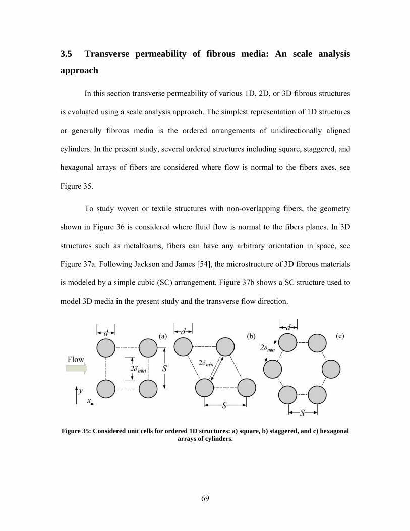
69
3.5 Transverse permeability of fibrous media: An scale analysis
approach
In this section transverse permeability of various 1D, 2D, or 3D fibrous structures
is evaluated using a scale analysis approach. The simplest representation of 1D structures
or generally fibrous media is the ordered arrangements of unidirectionally aligned
cylinders. In the present study, several ordered structures including square, staggered, and
hexagonal arrays of fibers are considered where flow is normal to the fibers axes, see
Figure 35.
To study woven or textile structures with non-overlapping fibers, the geometry
shown in Figure 36 is considered where fluid flow is normal to the fibers planes. In 3D
structures such as metalfoams, fibers can have any arbitrary orientation in space, see
Figure 37a. Following Jackson and James [54], the microstructure of 3D fibrous materials
is modeled by a simple cubic (SC) arrangement. Figure 37b shows a SC structure used to
model 3D media in the present study and the transverse flow direction.
Figure 35: Considered unit cells for ordered 1D structures: a) square, b) staggered, and c) hexagonal arrays of cylinders.
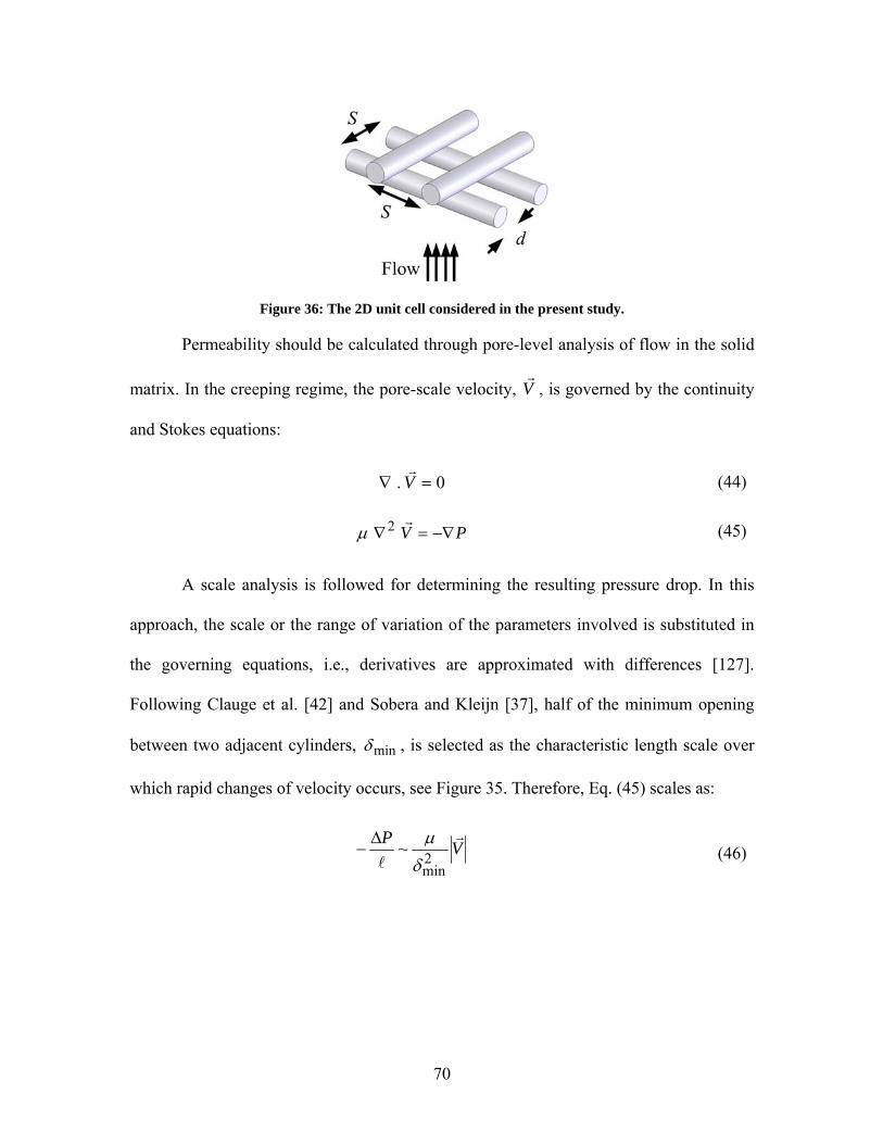
70
Figure 36: The 2D unit cell considered in the present study.
Permeability should be calculated through pore-level analysis of flow in the solid
matrix. In the creeping regime, the pore-scale velocity, V
, is governed by the continuity
and Stokes equations:
0. V
(44)
PV 2 (45)
A scale analysis is followed for determining the resulting pressure drop. In this
approach, the scale or the range of variation of the parameters involved is substituted in
the governing equations, i.e., derivatives are approximated with differences [127].
Following Clauge et al. [42] and Sobera and Kleijn [37], half of the minimum opening
between two adjacent cylinders, min , is selected as the characteristic length scale over
which rapid changes of velocity occurs, see Figure 35. Therefore, Eq. (45) scales as:
VP
2min
~
(46)

71
Figure 37: 3D structures; a) metalfoam, a real structure (scale bar is equal to 500 m ); b) simple
cubic arrangement, modeled unit cell used in the present analysis.
where is the characteristic length scale in the flow direction, see [37] for more details.
In case of non-touching cylinders with their axes perpendicular to the flow direction the
maximum velocity occurs in the section with minimum frontal area. Sobera and Klein
[37] proposed to use the average velocity in the section with minimum frontal area as the
characteristic velocity scale, i.e., /~ DUV
; where was the ratio of the minimum to
the total frontal areas in the unit cell. However, this assumption was only accurate for
highly porous structures, > 0.8, and overpredicted the pressure drop in low porosities
[37]. Carman [22] argued that a fluid particle should travel in a tortuous path of length
eL to pass through a sample of size L . Therefore, it is expected that the resulting

72
velocity scale for a constant pressure drop be inversely related to LLe / ; this ratio is
called the tortuosity factor, . Thus, the scale of the pore-level velocity magnitude
becomes:
DU
V ~
(47)
Substituting from Eq. (47) for velocity scale and using min as the length scale,
permeability can be calculated as:
2minCK
(48)
where C is a constant that should be determined through comparison with data.
Therefore one needs to know the ratio between the minimum to total frontal area, , and
the tortuosity factor, , to be able to calculate the permeability.
3.5.1 Tortuosity factor
The tortuosity factor is defined as the ratio of the average distance, eL , that a
particle should travel in a sample of size L . Due to its importance in mass, thermal and
electrical diffusion, several theoretical and empirical relationship have been proposed for
calculating the tortuosity in the literature; good reviews can be found elsewhere [128,
129]. Any relationship proposed for tortuosity should satisfy three conditions [128, 129]:
>1; 1lim 1; 0lim . One of the most popular empirical relationships for
determination of tortuosity, that satisfies all these conditions, is the Archie’s law [130]:

73
1
11
(49)
where is a constant and is the porosity. is a 'tuning' parameter that is found
through comparison of the Archie's empirical correlation, i.e., Eq. (49), with experimental
data. Boudreau [125], through comparison with data, showed that = 0.5 provides a
reasonable estimate for tortuosity in packed beds. The axes of fibers in 1D and 2D micro-
structures are perpendicular to the transverse flow direction which is similar to the flow
through packed beds of spherical particles. As a result, = 0.5 provides a good estimate
for the tortuosity of 1D and 2D structures as well. However; in 3D structures, some of the
fibers (roughly 1/3, consider an equally-spaced equally-sized cubic unit cell) are parallel
to the flow direction and do not affect the tortuosity of the medium. The study of
Tomadakis and Sotirchos [58] also showed that 3D fibrous structures are less tortuous in
comparison with 1D and 2D matrices. Consequently, an smaller than 0.5 should be
used for 3D microstructures. The deviation of Archie’s law with = 0.3 from the
tortuosity values predicted by the model of Tomadakis and Sotirchos [58] is less than
20%. In the present study, our model for permeability of 3D structures ( = 0.3) captures
the trends of the present experimental results and the data collected from various sources.
3.5.2 Experimental study
Experimental data for creeping flow through fibrous structures that we are
interested in is not abundant in the open literature. As such, several samples of tube banks
with 1D square and staggered fiber arrangements and metalfoams with 3D
microstructures shown in Figure 38 are tested using glycerol. To fabricate the tube bank

74
sample, Polymethyl methacrylate (PMMA) sheets of 3 mm thickness were cut and
drilled using a laser cutter with the accuracy of 0.05 mm . Glass capillary tubes with
diameter of 1.5 mm were inserted and fixed using an adhesive tape to form tube banks,
as shown in Figure 38. The length of the tube banks were selected such that a minimum
of 15 rows of cylinders existed in the flow direction for each sample. Aluminum 6101
metalfoam samples were purchased from ERG Duocel (Oakland, CA) with a number of
pores per inch (PPI) in the range of 10 to 40. The porosity of the samples was also
calculated independently by weighting the samples and measuring their volumes. In this
case, the density of the fibers was reported by manufacturer as 2690 kg/m3 and the solid
volume fraction was calculated as )volume2690/(mass . The fiber diameters were
estimated using SEM images and also compared with the data reported by others [131]
for similar materials. The properties of the samples are summarized in Table 7.
A custom-made gravity driven test bed, illustrated in Figure 38, was built that
included an elevated reservoir, an entry section, sample holder section, and an exit
section with a ball valve. The reservoir cross-section of 300300 mm2 was large enough
to ensure that the variation of the pressure head was negligible during the experiment.
The pressure drop across the samples was measured using a differential pressure
transducer, PX-154 (BEC Controls) with 1% accuracy. To minimize entrance and exit
effects on the pressure drop measurements, pressure taps were located few rows apart (at
least three rows) from the first and the last tube rows in the tube bank samples and 1 cm
apart from the sample edge for metalfoams. Glycerol was used as the testing fluid and the
bulk flow was calculated by weighting the collected test fluid over a period of time.
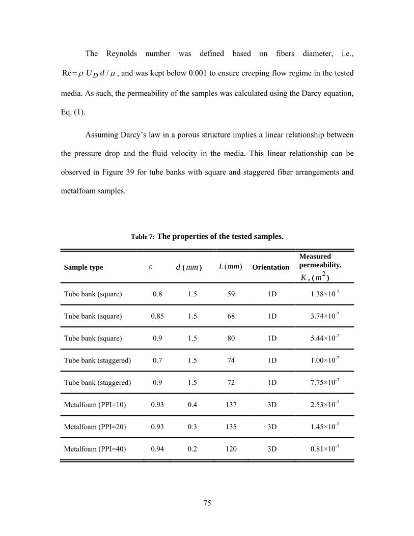
75
The Reynolds number was defined based on fibers diameter, i.e.,
/Re dU D , and was kept below 0.001 to ensure creeping flow regime in the tested
media. As such, the permeability of the samples was calculated using the Darcy equation,
Eq. (1).
Assuming Darcy’s law in a porous structure implies a linear relationship between
the pressure drop and the fluid velocity in the media. This linear relationship can be
observed in Figure 39 for tube banks with square and staggered fiber arrangements and
metalfoam samples.
Table 7: The properties of the tested samples.
Sample type d ( mm ) )(mmL Orientation
Measured permeability,
K , (2m )
Tube bank (square) 0.8 1.5 59 1D 1.38×10⁻⁷
Tube bank (square) 0.85 1.5 68 1D 3.74×10⁻⁷
Tube bank (square) 0.9 1.5 80 1D 5.44×10⁻⁷
Tube bank (staggered) 0.7 1.5 74 1D 1.00×10⁻⁷
Tube bank (staggered) 0.9 1.5 72 1D 7.75×10⁻⁷
Metalfoam (PPI=10) 0.93 0.4 137 3D 2.53×10⁻⁷
Metalfoam (PPI=20) 0.93 0.3 135 3D 1.45×10⁻⁷
Metalfoam (PPI=40) 0.94 0.2 120 3D 0.81×10⁻⁷

76
3.5.3 Results and discussion
Equation (48) relates the permeability of fibrous media to the minimum opening between
adjacent fibers, min , the ratio between minimum to total frontal area, , and tortuosity
factor, , that can be calculated from Eq. (49). In the following subsections, using
geometrical properties of the considered microstructures, compact models will be
developed that relate the permeability to the solid volume fraction.
3.5.3.1 Unidirectionally Aligned Arrangements
For the three different ordered 1D unit cells shown in Figure 35, it can be seen
that SdS /)( and 2/)(min dS . Therefore, Eq. (48) can be rewritten as:
1
3
S
dSCK
(50)
Combining Eqs. (28) and (50), the dimensionless permeability of the ordered
structures becomes:
Hexagonal1
333
333
3316.0
Staggered1
323
323
3216.0
Square1
43
43
416.0
2
d
K
(51)
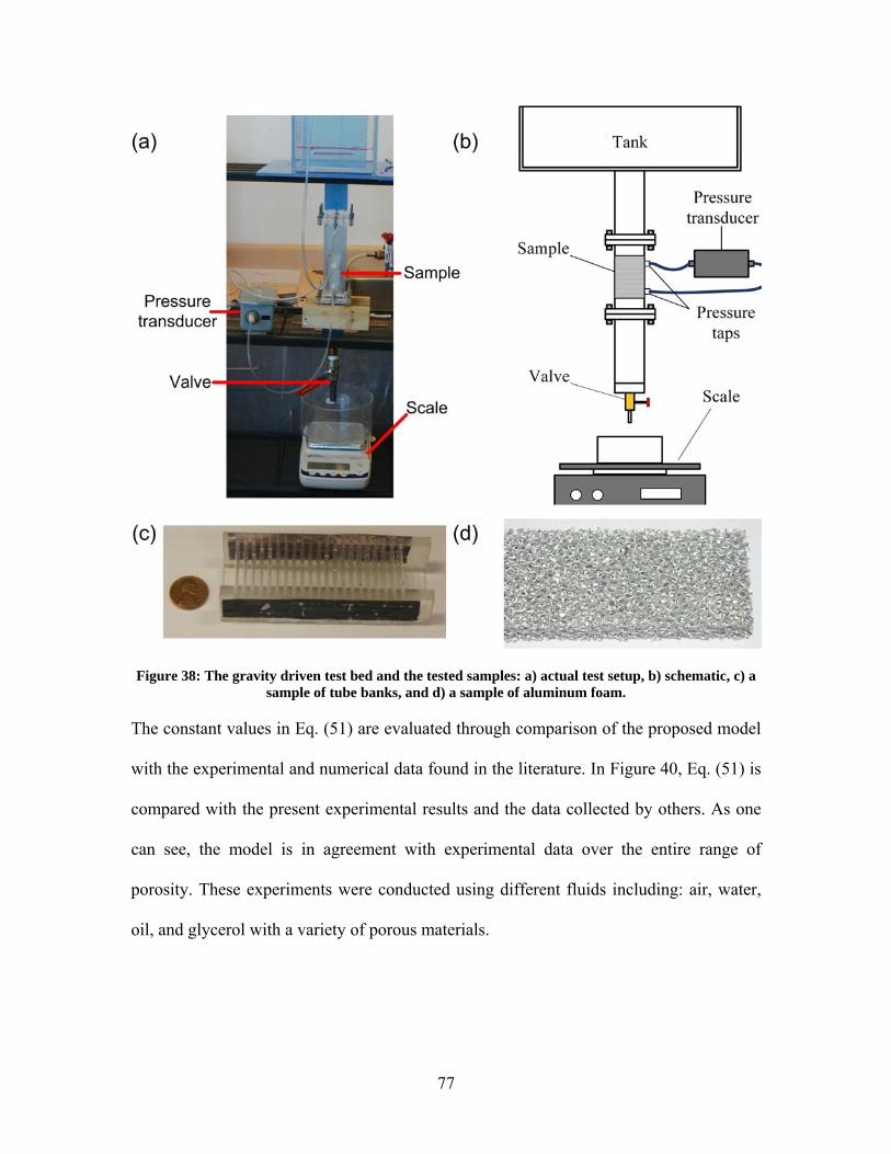
77
Figure 38: The gravity driven test bed and the tested samples: a) actual test setup, b) schematic, c) a sample of tube banks, and d) a sample of aluminum foam.
The constant values in Eq. (51) are evaluated through comparison of the proposed model
with the experimental and numerical data found in the literature. In Figure 40, Eq. (51) is
compared with the present experimental results and the data collected by others. As one
can see, the model is in agreement with experimental data over the entire range of
porosity. These experiments were conducted using different fluids including: air, water,
oil, and glycerol with a variety of porous materials.

78
Figure 39: measured pressure gradients for samples of a) tube bank with square fiber arrangement, b) tube bank with staggered fiber arrays, and c) metalfoams.
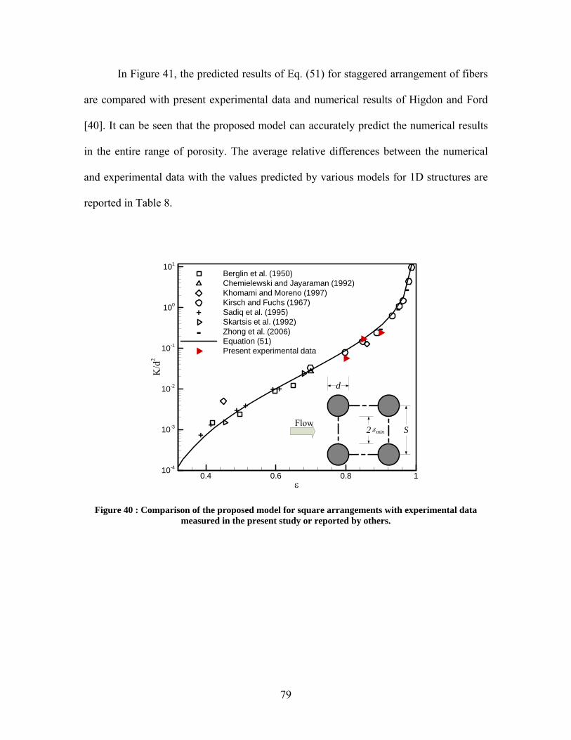
79
In Figure 41, the predicted results of Eq. (51) for staggered arrangement of fibers
are compared with present experimental data and numerical results of Higdon and Ford
[40]. It can be seen that the proposed model can accurately predict the numerical results
in the entire range of porosity. The average relative differences between the numerical
and experimental data with the values predicted by various models for 1D structures are
reported in Table 8.
++
+ +
+ +
--
-
K/d
2
0.4 0.6 0.8 110-4
10-3
10-2
10-1
100
101
Berglin et al. (1950)Chemielewski and Jayaraman (1992)Khomami and Moreno (1997)Kirsch and Fuchs (1967)Sadiq et al. (1995)Skartsis et al. (1992)Zhong et al. (2006)Equation (51)Present experimental data
+
-
Figure 40 : Comparison of the proposed model for square arrangements with experimental data measured in the present study or reported by others.
S
d
Flow2 min
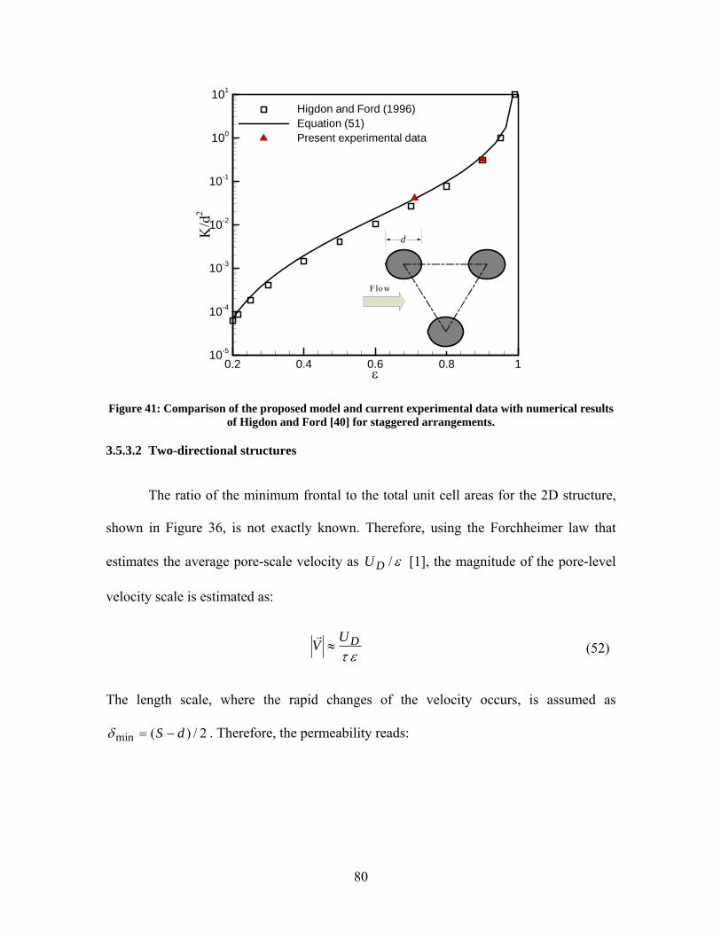
80
K/d
2
0.2 0.4 0.6 0.8 110-5
10-4
10-3
10-2
10-1
100
101
Higdon and Ford (1996)Equation (51)Present experimental data
Figure 41: Comparison of the proposed model and current experimental data with numerical results of Higdon and Ford [40] for staggered arrangements.
3.5.3.2 Two-directional structures
The ratio of the minimum frontal to the total unit cell areas for the 2D structure,
shown in Figure 36, is not exactly known. Therefore, using the Forchheimer law that
estimates the average pore-scale velocity as /DU [1], the magnitude of the pore-level
velocity scale is estimated as:
DU
V
(52)
The length scale, where the rapid changes of the velocity occurs, is assumed as
2/)(min dS . Therefore, the permeability reads:
d
Flow

81
Table 8: The average relative difference between the permeability values predicted by different models with the numerical and experimental data for 1D square, 1D staggered, and 3D simple cubic
structures over the entire range of porosity.1
1D square arrays (compared to experimental data)
Author(s) Relative
difference (%)
Author(s) Relative
difference (%)
Equation (23) 24.9 Happel (1959) 47.5
Gebart (1992) 26.8 Drummond and Tahir (1984) 245.2
Van der Westhuizen (1996) 45.8 Equation (51) 15.8
Sahraoui and Kaviany (1994) 25.6
1D staggered arrays (compared to present experimental data and numerical results of Higdon and Ford [40])
Author(s) Relative
difference (%)
Author(s) Relative
difference (%)
Gebart (1992) 11.6 Equation (51) 26.6
Happel (1959) 38.8
3D simple cubic structure (Compared to numerical results of Higdon and Ford [40])
Author(s) Relative
difference (%)
Author(s) Relative
difference (%)
Tomadakis and Robertson (2005)
24.9 Equation (55) 19.3
Jackson and James (1986) 247.3
1 Relative difference = /modeldatamodel
2dSCK
(53)
Substituting for geometrical parameters from Eq. (41) and the tortuosity from Archie’s
law, the dimensionless permeability becomes:
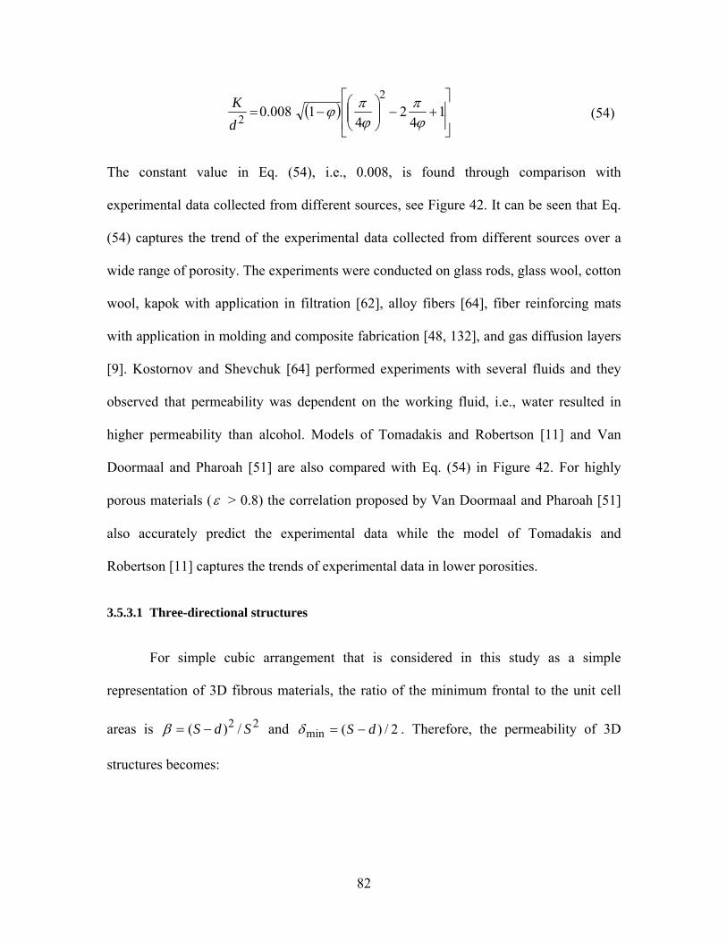
82
1
42
41008.0
2
2
d
K
(54)
The constant value in Eq. (54), i.e., 0.008, is found through comparison with
experimental data collected from different sources, see Figure 42. It can be seen that Eq.
(54) captures the trend of the experimental data collected from different sources over a
wide range of porosity. The experiments were conducted on glass rods, glass wool, cotton
wool, kapok with application in filtration [62], alloy fibers [64], fiber reinforcing mats
with application in molding and composite fabrication [48, 132], and gas diffusion layers
[9]. Kostornov and Shevchuk [64] performed experiments with several fluids and they
observed that permeability was dependent on the working fluid, i.e., water resulted in
higher permeability than alcohol. Models of Tomadakis and Robertson [11] and Van
Doormaal and Pharoah [51] are also compared with Eq. (54) in Figure 42. For highly
porous materials ( > 0.8) the correlation proposed by Van Doormaal and Pharoah [51]
also accurately predict the experimental data while the model of Tomadakis and
Robertson [11] captures the trends of experimental data in lower porosities.
3.5.3.1 Three-directional structures
For simple cubic arrangement that is considered in this study as a simple
representation of 3D fibrous materials, the ratio of the minimum frontal to the unit cell
areas is 22 /)( SdS and 2/)(min dS . Therefore, the permeability of 3D
structures becomes:

83
-
--
-
++
++
+
++
+++
K/d
2
0.5 0.6 0.7 0.8 0.9 110-3
10-2
10-1
100
101 Davies (1952)Molnar et al. (1989)Kostornov and Shevchuk (1977)Gostick et al. (2006)Zobel et al. (2007)VanDoormaal and Pharoah (2008)Tomadakis and Robertson (2005)Equation (54)
-+
Figure 42: Comparison of the present model, models of Van Doormaal and Pharoah [51] and
Tomadakis and Robertson [11] with experimental data for transverse permeability of 2D structures.
3.022
4
208.0
dS
dS
d
K
(55)
where the relationship between geometrical parameters of SC structure is:
3
3
2
22
4
3
S
d
S
d
(56)
The constant in Eq. (55) is found to be 0.08 through comparison of this equation
with the numerical data reported by Higdon and Ford [40] for SC arrangements over a
wide range of porosity. Figure 43 includes the present model, models of Tomadakis and
Robertson [11] and Jackson and James [54], current experimental measurements, and
experimental data collected from different sources. The plotted data are based on the
permeability values reported for polymer chain in solutions [65], glass wool randomly

84
++ +++
+++
+++ ++++
+ +++ +++
K/d
2
0.5 0.6 0.7 0.8 0.9 110-3
10-2
10-1
100
101
102
Jackson and James (1982)Carman (1938)Rahli (1997)Bhattacharya et al. (2002)Higdon and Ford (1996), numericalJackson and James (1986)Tomadakis and Sotirchos (1993)Present experimental dataEquation (55)
+
Figure 43: Comparison of the proposed model for 3D structures, models of Jackson and James [54] and Tomadakis and Robertson [11], present experimental results and data reported by others.
packed, stainless steel crimps [22], metallic fibers [69], and aluminum metalfoams [94].
It can be seen that the present model is in agreement with the experimental data and
numerical results collected from a number of studies over the entire range of porosity.
The average relative differences between the numerical data reported by Higdon and Ford
[40] and Eq. (55), the model of Tomadakis and Robertson [11], and the model of Jackson
and James [54] are listed in Table 8.
3.6 Through-plane permeability of carbon papers
Through-plane permeability of uncompressed carbon papers with no PTFE
treatment can be estimated using the existing models for the permeability of planar
fibrous structures. Based on the analogy between electrical and flow conductions,
Tomadakis and Robertson [11] developed a model for permeability of randomly
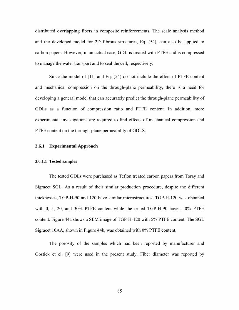
85
distributed overlapping fibers in composite reinforcements. The scale analysis method
and the developed model for 2D fibrous structures, Eq. (54), can also be applied to
carbon papers. However, in an actual case, GDL is treated with PTFE and is compressed
to manage the water transport and to seal the cell, respectively.
Since the model of [11] and Eq. (54) do not include the effect of PTFE content
and mechanical compression on the through-plane permeability, there is a need for
developing a general model that can accurately predict the through-plane permeability of
GDLs as a function of compression ratio and PTFE content. In addition, more
experimental investigations are required to find effects of mechanical compression and
PTFE content on the through-plane permeability of GDLS.
3.6.1 Experimental Approach
3.6.1.1 Tested samples
The tested GDLs were purchased as Teflon treated carbon papers from Toray and
Sigracet SGL. As a result of their similar production procedure, despite the different
thicknesses, TGP-H-90 and 120 have similar microstructures. TGP-H-120 was obtained
with 0, 5, 20, and 30% PTFE content while the tested TGP-H-90 have a 0% PTFE
content. Figure 44a shows a SEM image of TGP-H-120 with 5% PTFE content. The SGL
Sigracet 10AA, shown in Figure 44b, was obtained with 0% PTFE content.
The porosity of the samples which had been reported by manufacturer and
Gostick et el. [9] were used in the present study. Fiber diameter was reported by

86
Table 9: Physical properties of different carbon papers used in the present study: porosity and PTFE
content provided by the manufacturers; the measured thicknesses and fiber diameters.
GDL Thickness ( m ) Porosity*
Fiber diameter ( m )
PTFE content (%)
SGL-Sigracet 10AA
390-410 0.88 9.2 0
TGP-H-90 255-270 0.79 9.3 0
TGP-H-120 370-385 0.79 9.3 0-30
*The porosity is reported for GDLs with 0% PTFE content.
Gostick et al. [9] and was also independently calculated using scanning electron
microscopy (SEM) images. The thickness of the samples was measured using a
micrometer; the maximum uncertainty associated with the measurements is less than
10 m . The properties of the purchased samples are listed in Table 9.
3.6.1.2 Test apparatus
An air permeability test bed was designed and built for measuring the through-
plane permeability, see Figure 45. The high pressure air was supplied by a high pressure
air tank and controlled using a digital air pressure regulator; the output pressure of the air
regulator valve was set to 6 psi during all experiments. Two aluminum blocks were
machined and drilled with a 25mm diameter hole. The blocks were used as sample
holders and the GDL samples were sandwiched between the blocks. An O-ring was used
between the two aluminum blocks to prevent air leakage from the test section.

87
Figure 44: SEM Images: a) TGP 120 with 5% PTFE content; b) SGL Sigracet 10AA; c) compressed TGP 120 with 5% PTFE content.
The up and down stream air flow were connected to a differential pressure
transducer, PX277-01D5V, supplied by Omega (Omega Inc., Laval, QC, Canada). The
pressure transducer was connected to a PC, using a DAQ purchased from Omega (Omega
Inc., Laval, QC, Canada), where the pressure drop values were recorded. The accuracy of
the pressure transducer was 1% of its full scale measuring range (0-1 inch of water). The
air flow rate passing through the GDLs was measured using a flow meter provided by
Omega (Omega Inc., Laval, QC, Canada). The accuracy and the range of the air flow
meter was 3% and 0-10 lpm, respectively.

88
The carbon papers were cut into circular samples of 3 cm diameter for the
experiments. To investigate the compression effects, GDL samples were compressed
using a GUNT WP 300 Universal Material Tester for 15 min; the maximum applied
compressive force was less than 20 kN. The thickness of the compressed samples was
measured after the load was released to determine the variation in its thickness, using the
same micrometer.
3.6.1.3 Data analysis
Gas permeability, K, is defined using Darcy equation:
DUKt
P
(57)
where DU is the volume averaged velocity through porous media, is viscosity, P is
the pressure drop across the sample, and t is the GDLs thickness. Darcy equation is valid
for incompressible, steady, constant properties, single-phase (no-surface tension forces),
and low Reynolds number flows.
The Reynolds number based on the fiber diameter, /Re dUD , was lower
than 0.1 in the present study; therefore, the Darcy equation was applicable for analyzing
the experimental results. The maximum measured pressure drop across the samples was
less than 200 Pa. As such, it was assumed that the compressibility effects for such small
values of pressure drop can be negligible and the Darcy equation in the form of Eq. (57)
was applicable in the present study. DU was calculated by dividing the volumetric flow
rate by the sample cross-sectional area.

89
Figure 45: The air permeability test bed: a) schematic of the apparatus (exploded view) b) actual test setup.
Assuming Darcy’s law in a porous structure implies a linear relationship between
the pressure drop and the fluid velocity in the media. As an example, this linear

90
relationship can be observed in the experimental results for samples of compressed TGP-
H-120 in Figure 46 which justifies Darcy’s assumptions.
The measured values of pressure drop, totalP , during the experiments were:
minsampletotal PPP
(58)
where sampleP is the pressure drop associated with the sample and minP is the
pressure drop due to minor losses in the testbed, i.e., exit and entrance section of the
sample holder. To account for the minor pressure losses, the pressure drop in the test
section was measured once without any GDL samples to determine minP for the entire
range of flow rate considered in the present experimental work.
UD
p/t
0 0.05 0.1 0.15 0.2
2.0x10+05
4.0x10+05
6.0x10+05
8.0x10+05
TGp-H-120, = 0.80TGp-H-120, = 0.78TGp-H-120, = 0.76TGp-H-120, = 0.72
PTFE % = 0%
Figure 46: Measured pressure drops for samples of compressed TGP-H-120.

91
The uncertainty associated with the through-plane permeability, calculated based
on the measured variables using the Darcy’s equation, can be estimated from[133]:
222 )()()()(
D
DU
UE
P
PE
t
tE
K
KE
(59)
where (.)E is the uncertainty in the measurement of each parameter; these values are
listed in Table 10. The maximum uncertainty in the calculated values of permeability is
estimated to be 9%.
3.6.2 Theoretical Model
Our scale analysis model, Eq. (54) was successfully compared with experimental
data collected from various sources. The tortuosity factor used in derivation of Eq. (54) is
based on the Bruggeman equation [134]. Hao and Cheng [49] numerically calculated the
tortuosity factor for carbon papers and proposed the following correlation:
54.011.0
172.01
(60)
Table 10: Uncertainty values for measured parameters
Parameter Uncertainty 10 m
P 1% of full scale
DU 3% of full scale
5%
K 9%

92
Our analysis showed that if the constant value in Eq. (54) is replaced by 0.012 and
is calculated from Eq. (60) the resulting equation:
54.0
2
2 89.072.011
42
41012.0
d
K
(61)
can predict the experimental data for GDLs more accurately. To enable Eq. (61) to
include the effects of compression factor and PTFE content, the relationship between
these properties and the solid volume fraction should be determined.
Figure 44c shows that mechanical compression does not change the shape of
fibers. It can be assumed that during the compression process only the thickness of the
original fibrous samples changes while the volume of the solid carbon fiber remains
constant. Therefore, the relationship between the solid volume fraction, comp , of a
compressed sample with the original value for an uncompressed carbon paper, 0 , can be
expressed as [49]:
compcomp t
t00
(62)
where compt and 0t are the compressed and uncompressed GDL thicknesses,
respectively. If the PTFE is added on the carbon paper GDL, the pore volume is
randomly filled by the PTFE. It is postulated that PTFE changes the porosity and some
pores in the medium are filled. The final porosity, PTFE , can be expressed
approximately as a function of PTFE content [49]:
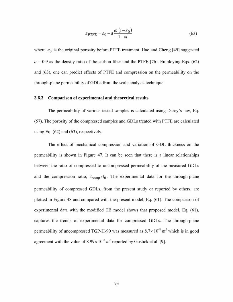
93
1
1 00 aPTFE
(63)
where 0 is the original porosity before PTFE treatment. Hao and Cheng [49] suggested
a = 0.9 as the density ratio of the carbon fiber and the PTFE [76]. Employing Eqs. (62)
and (63), one can predict effects of PTFE and compression on the permeability on the
through-plane permeability of GDLs from the scale analysis technique.
3.6.3 Comparison of experimental and theoretical results
The permeability of various tested samples is calculated using Darcy’s law, Eq.
(57). The porosity of the compressed samples and GDLs treated with PTFE are calculated
using Eq. (62) and (63), respectively.
The effect of mechanical compression and variation of GDL thickness on the
permeability is shown in Figure 47. It can be seen that there is a linear relationships
between the ratio of compressed to uncompressed permeability of the measured GDLs
and the compression ratio, 0/ ttcomp . The experimental data for the through-plane
permeability of compressed GDLs, from the present study or reported by others, are
plotted in Figure 48 and compared with the present model, Eq. (61). The comparison of
experimental data with the modified TB model shows that proposed model, Eq. (61),
captures the trends of experimental data for compressed GDLs. The through-plane
permeability of uncompressed TGP-H-90 was measured as 8.710-8 m2 which is in good
agreement with the value of 8.9910-8 m2 reported by Gostick et al. [9].

94
t uncomp / t0
K/K
un
com
p
0.4 0.6 0.8 10.2
0.4
0.6
0.8
1TGP-H-120
TGP-H-90
SGL- 10 AA
Figure 47: Effect of compression ratio, 0/ ttcomp on the variation of permeability.
++++
K/d
2
0.6 0.7 0.8 0.910-2
10-1
100
101
Gostick et al. (2006)Becker et al. (2009)Tahlar et al. (2010)Present study, SGL 10 AAPresent study, TGP-H-90Present study, TGP-H-120TB model, Eqs. (61-63)
+
Figure 48: Comparison of the proposed model with the experimental data for compressed GDLs
measured in the present study or collected from various sources.

95
The effect of PTFE content on the through-plane permeability of GDLs is
presented in Figure 49. It can be seen that a reverse relationship exist between the PTFE
content and the through-plane permeability. The experimental data for TGP-H-120 with
various PTFE contents are plotted in Figure 50 and compared with TB model. Porosities
of the samples are estimated from Eq. (63). The permeability of the PTFE treated GDLs
has a reverse relationship with the PTFE content. It can be seen that Eq. (61) predicts the
reverse relationship between permeability and PTFE contents; this is in agreement with
the experimental data. Overall, it can be concluded that the modified TB model can be
used in design and optimization process of PEMFCs.
PTFE (%)
K/K
no
ntr
eate
d
K/d
2
0 10 20 300.5
0.6
0.7
0.8
0.9
1
0
0.1
0.2
0.3
K / Knon treated, TGP-H-120
K / d2, TGP-H-120
Figure 49: Effect of PTFE content on the through-plane permeability of two set of TGP-H-120 samples with various PTFE contents.
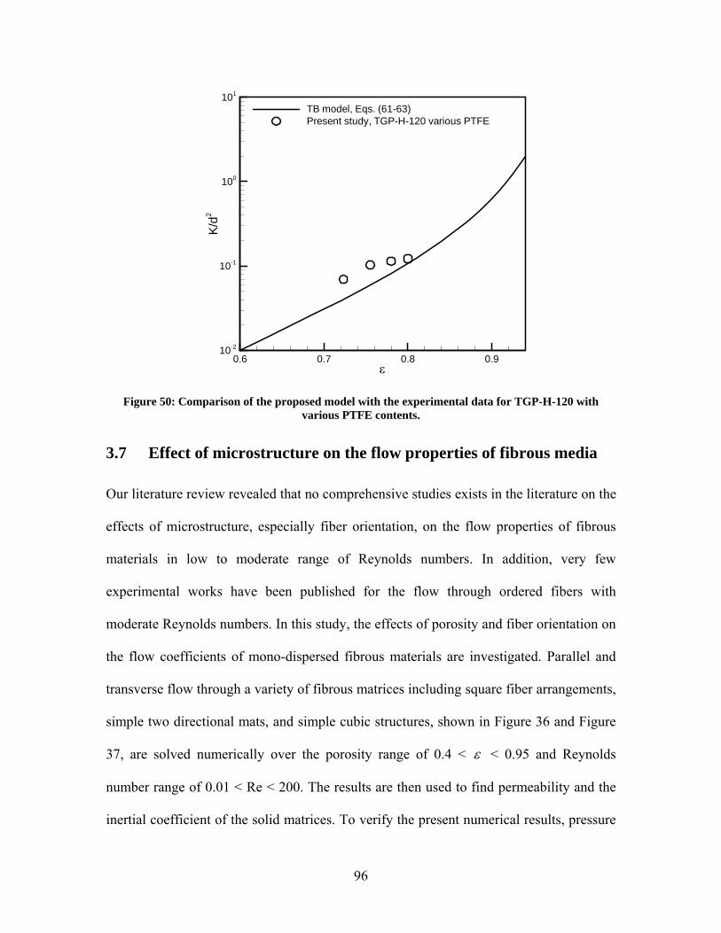
96
K/d
2
0.6 0.7 0.8 0.910-2
10-1
100
101
TB model, Eqs. (61-63)Present study, TGP-H-120 various PTFE
Figure 50: Comparison of the proposed model with the experimental data for TGP-H-120 with various PTFE contents.
3.7 Effect of microstructure on the flow properties of fibrous media
Our literature review revealed that no comprehensive studies exists in the literature on the
effects of microstructure, especially fiber orientation, on the flow properties of fibrous
materials in low to moderate range of Reynolds numbers. In addition, very few
experimental works have been published for the flow through ordered fibers with
moderate Reynolds numbers. In this study, the effects of porosity and fiber orientation on
the flow coefficients of mono-dispersed fibrous materials are investigated. Parallel and
transverse flow through a variety of fibrous matrices including square fiber arrangements,
simple two directional mats, and simple cubic structures, shown in Figure 36 and Figure
37, are solved numerically over the porosity range of 0.4 < < 0.95 and Reynolds
number range of 0.01 < Re < 200. The results are then used to find permeability and the
inertial coefficient of the solid matrices. To verify the present numerical results, pressure

97
drop through three different tube banks with porosity range of 0.8 < < 0.9 are tested
using various water-glycerol mixtures to determine the flow coefficients.
If the pore sizes are much larger than the molecular mean free path, flow in pore
scale is governed by Navier-Stokes equation; that is the continuum flow hypothesis
which is considered here. Assuming incompressible, steady state flow, the microscopic
equations become [118]:
0. V
(64)
VPVV 2.
(65)
where V
is the pore scale velocity vector, and are the fluid density and viscosity,
respectively. Eqs. (64) and (65) are subject to no-slip boundary condition at the fibers’
surface. After volume averaging, Eq. (65) leads to Eq. (2) and in the creeping flow limit,
reduces to Eq. (1). Equation (2) is usually written in the following form [1]:
2DD U
K
FU
KP
(66)
where F is a dimensionless number called the Forchheimer coefficient. A special form of
Eq. (66) is the Ergun equation:
2323
2 175.1
1150 DD U
dU
dP
(67)
where 223 1150/ dK and 2/3/14.0 F . Ergun equation is based on a curve fit
of experimental data collected for granular materials [1].
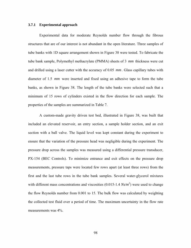
98
3.7.1 Experimental approach
Experimental data for moderate Reynolds number flow through the fibrous
structures that are of our interest is not abundant in the open literature. Three samples of
tube banks with 1D square arrangement shown in Figure 38 were tested. To fabricate the
tube bank sample, Polymethyl methacrylate (PMMA) sheets of 3 mm thickness were cut
and drilled using a laser cutter with the accuracy of 0.05 mm . Glass capillary tubes with
diameter of 1.5 mm were inserted and fixed using an adhesive tape to form the tube
banks, as shown in Figure 38. The length of the tube banks were selected such that a
minimum of 15 rows of cylinders existed in the flow direction for each sample. The
properties of the samples are summarized in Table 7.
A custom-made gravity driven test bed, illustrated in Figure 38, was built that
included an elevated reservoir, an entry section, a sample holder section, and an exit
section with a ball valve. The liquid level was kept constant during the experiment to
ensure that the variation of the pressure head was negligible during the experiment. The
pressure drop across the samples was measured using a differential pressure transducer,
PX-154 (BEC Controls). To minimize entrance and exit effects on the pressure drop
measurements, pressure taps were located few rows apart (at least three rows) from the
first and the last tube rows in the tube bank samples. Several water-glycerol mixtures
with different mass concentrations and viscosities (0.015-1.4 Ns/m2) were used to change
the flow Reynolds number from 0.001 to 15. The bulk flow was calculated by weighting
the collected test fluid over a period of time. The maximum uncertainty in the flow rate
measurements was 4%.

99
To obtain the permeability and the inertial coefficient from the measured pressure
drop dxdp / and mass flow rate values, the volume averaged superficial velocity, DU ,
was calculated from the mass flow rate data and then DUdxdp // was plotted versus
/DU . The y-intercept and the slope of the data were then K/1 and KF / ,
respectively; see Eq. (66). Using Eq. (2), the inertial coefficient was then calculated.
From Figure 51, it can be seen that the measured pressure drops present a parabolic
relationship with the volume-averaged velocity.
The uncertainty associated with the permeability and inertial coefficient,
calculated based on the measured variables, can be estimated as:
22
/
)/(
/
)/(
,
),(
D
D
D
DULP
ULPE
U
UE
K
KE
(68)
where:
222)()()(
/
)/(
E
U
UEE
U
UE
D
D
D
D
(69)
222)()(
/
)/(
/
)/(
E
U
UE
LP
LPE
ULP
ULPE
D
D
D
D
(70)
(.)E is the uncertainty in measurement of each parameter; these values are listed in Table
11. The maximum uncertainty in the experimental values of permeability and inertial
coefficient is estimated to be 12%.

100
UD /
(dP
/dx)
/(
UD)
2000 4000 6000 8000
3.0x10+06
6.0x10+06
9.0x10+06
= 0.8 = 75
= 0.85 = 35.8
= 0.9 = 26.7
Figure 51: Measured values of dxdpUD //1 for the samples of tube bank with square fiber
arrangement.
Table 11: Uncertainty in the measured parameters.
Parameter Uncertainty 3%
LP / 1% of full scale
Q 4% of full scale
DU 4%
K 12%
12%
3.7.2 Numerical procedure
Equations (64) and (65) are solved using Fluent [122] which is a finite volume
based software. The second order upwind scheme is selected to discretize the governing
equations and SIMPLE algorithm [123] is employed for pressure-velocity coupling. The
inlet and outlet boundaries of the computational domains are considered to be periodic,

101
i.e., the velocity distributions on both boundaries are the same [122]. The symmetry
boundary condition is applied on the side borders of the considered unit cells; this means
that normal velocity and gradient of parallel component of the velocity on the side
borders are zero. However, for three dimensional cases, employing the periodic condition
leads to a poor convergence rate. As a result of our limited computational resources, in
some cases, a set of 7-10 unit cells in series are considered and velocity profiles are
compared at the entrance to each unit cell. For these cases, the inlet velocity of the media
is assumed to be uniform. Constant pressure boundary condition is applied on the
computational domain outlet. The pressure drops used for calculation of flow properties
are only the values obtained from the developed regions.
Structured grids and unstructured grids are generated for 1D/2D and 3D networks,
respectively, using Gambit [122], the pre-processor in Fluent software. Numerical grid
aspect ratios are kept in the range of 1-7. Grid independence is tested for different cases
and the size of the computational grids used for each geometry is selected such that the
maximum difference in the predicted values for pressure gradient is less than 2%. The
maximum number of grids used for 1D and 2D/3D structures are approximately 14k and
1,400k, respectively. It should be noted that the convergence criterion, maximum relative
error in the value of dependent variables between two successive iterations, is set at 10-6.
In this part, numerical simulations are carried out for fibrous networks in the
porosity range of 0.3 - 0.95 and in the Reynolds number range of 0.001 – 200. SC
arrangements are orthotropic while the rest of the considered structures are anisotropic
[11]. Therefore, numerical simulations are conducted for flow parallel to different
coordinate axes. The same method as described in the previous section is employed to
102
determine the permeability and the inertial/Forchheimer coefficient from numerical
results for different unit cells. The summary of the computed flow coefficients are
reported in Table 12.
Flow parallel to axes of square arrays of cylinders is similar to laminar channel
flows. This leads to zero value for Forchheimer coefficient in parallel flow as reported in
Table 12. Similarly, for 2D structures, the in-plane Forchheimer coefficients have lower
values than the calculated values for through-plane flow. This is resulted from the fact
that 50% of the fibers in the considered geometry are parallel to the flow direction.
Therefore, no inertial drag forces are exerted on these fibers.
3.7.3 Comparison of the numerical results with existing data in the literature
3.7.3.1 Square arrangement (1D)
To validate the numerical analysis, the calculated values of the dimensionless
normal permeability, 2/ dK , are successfully compared with present experimental results
and the data collected from several sources in Figure 52. Moreover, in Figure 53, the
calculated Forchheimer coefficients for square arrangements are compared with the
present experimental data, the numerical results of Ghaddar [84] and Papathanasiou et al.
[85] for monodisperse and bimodal fiber arrays, respectively. In addition, the
experimental data of Bergelin et al. [61] (oil flowing across tube banks) are included in
Figure 53. In general, the present results are in good agreement with the collected and
reported data by others.

103
Table 12: Flow properties for the considered fibrous structures.
Square array (1D)
Normal flow Parallel flow
2/ dK F 2/ dK F
0.45 0.0015 0.13 0.45 0.0079 0
0.65 0.014 0.026 0.55 0.0177 0
0.8 0.072 0.018 0.65 0.0378 0
0.9 0.300 0.011 0.8 0.1667 0
0.95 0.892 0.009 0.9 0.643 0
Planar structures (2D)
Through plane flow In-plane flow
2/ dK F 2/ dK F
0.35 0.0007 0.313 0.35 0.0016 0.092
0.5 0.0046 0.118 0.5 0.0069 0.046
0.6 0.012 0.091 0.6 0.0164 0.033
0.8 0.106 0.033 0.8 0.0807 0.018
0.9 0.439 0.0028 0.9 0.4119 0.013
Simple cubic (3D)
2/ dK F
0.31 0.0011 0.914
0.37 0.0023 0.562
0.59 0.0174 0.141
0.79 0.118 0.041
0.87 0.336 0.024

104
+
+
+
K/d
2
0.4 0.6 0.8 1
10-3
10-2
10-1
100
101
Bergelin et al. (1950)Kirsch and Fuchs (1967)Sadiq et al. (1995)Khomami and Moreno (1997)Zhong et al. (2006)Present experimental resultsPresent numerical results
+
Figure 52: Comparison between the present numerical results, collected experimental results, and data from various sources, for normal flow through square fiber arrays.
F
0.4 0.5 0.6 0.7 0.8 0.90
0.05
0.1
0.15
0.2
0.25
0.3
Papathanasiou et al. (2001)Ghaddar et al. (1995)Berglin et al. (1950), experimentalPresent experimental dataPresent numerical results
Inertial coefficient, square arrangements
Figure 53: Comparison between the present numerical and experimental results for Forchheimer coefficient with experimental and numerical data of others.

105
3.7.3.2 2D and 3D simple cubic structures
There is no experimental data for moderate Reynolds number flows through the
ordered 2D and 3D structures considered in the present study. To validate the analysis,
the calculated permeability values for simple cubic arrangement are compared with the
numerical results of Higdon and Ford [40] and experimental data for actual 3D materials
with random fiber distribution collected from different sources in Figure 54. The plotted
data are based on permeability results for polymer chain in solutions [65], glass wool
randomly packed, stainless steel crimps [22], metallic fibers [69], and aluminum metal
foams [94, 135].
3.7.4 Effects of microstructure on flow properties
Effects of microstructure and more specifically fibers orientation on permeability
and Forchheimer coefficient are investigated in Figure 55 and Figure 56, respectively. As
expected, 1D arrangements are the most anisotropic geometry and the normal and parallel
permeability of such structures provide the lower and upper bounds for permeability of
fibrous media. Effects of microstructure are more pronounced in lower porosities.
The plotted data in Figure 56 indicates that 1D and 2D geometries are anisotropic
and the Forchheimer coefficient for 3D structures is higher than values for 1D and 2D
geometries. The Forchheimer coefficient is a measure of inertial effects. Thus, it is more
influenced by microstructure in the porosity range of < 0.7.

106
++
++
+++
++
++
++
++
K/d
2
0.4 0.6 0.8
10-3
10-2
10-1
100
101
Jackson and James (1982)
Carman (1938)
Rahli (1997)
Bhattacharya et al. (2002)
Higdon and Ford (1996), numerical
Tamayol and Bahrami (2010)
Present numerical results
+
Figure 54: Comparison between the present numerical results for permeability of simple cubic arrangements with existing numerical and experimental data of 3D materials.
++
+
+
+
K/d
2
0.3 0.4 0.5 0.6 0.7 0.8 0.9
10-3
10-2
10-1
100
101
102
Ergun equation1D square arrays, normal flow1D square arrays, parallel flow2D structures, through plane flow2D structures, in-plane flow3D simple cubic strucutre+
Figure 55: Comparison of numerical values of dimensionless permeability of fibrous media with Ergun equation.

107
+
+
+
+ +
F
0.3 0.4 0.5 0.6 0.7 0.8 0.90
0.25
0.5
0.75
1Ergun equation1D square arrays, normal flow2D structures, through plane flow2D structures, in-plane flow3D simple cubic strucutre+
Figure 56: Comparison of numerical values of Forchheimer coefficient of fibrous media with Ergun equation.
Ergun equation, Eq. (67), is a widely accepted equation for prediction of pressure
drop across granular materials. However; there are two main differences between fibrous
and granular materials are:
Shape of the particles in granular materials is spherical while fibrous
media are made up of cylindrical like particles.
Porosity of granular materials are in the range of 0.2 – 0.6, while the
porosity of fibrous materials usually is in the range of 0.6 - 0.999.
The present numerical results are compared with the values predicted by the
Ergun equation to investigate the accuracy of this equation for high porosity fibrous
structures. Figure 55 includes the predicted values of permeability from Ergun equation
and the present numerical results. It can be seen that the Ergun equation can only predict
trends of numerical data qualitatively and the differences are significant especially in low

108
porosities. The Forchheimer results calculated from the Ergun equation are plotted
against the current numerical results in Figure 56. The comparison shows that the Ergun
equation is only in agreement with numerical results for 3D materials with low porosities.
For higher porosities Eq. (67) is incapable of predicting the pressure drop for fibrous
media.
Creeping flow through fibrous media has been investigated in the previous
subsections and accurate models have been proposed for calculating the permeability.
However, no compact relationships exist for estimating the Forchheimer coefficient of
various fibrous structures. Using our numerical results, a series of compact correlations
are developed for 1D, 2D, and 3D fibrous structures and are listed in Table 13. The
proposed correlations are accurate within 2% of the present numerical results.
Table 13: Proposed compact correlations for Forchheimer coefficient in fibrous media.
Flow direction/microstructure cbaF /1
a b c
Normal/square arrays (1D) -5.32 18.42 0.532
Through plane- 2D structures -0.14 5.05 0.418
In-plane/2D structures 1.037 0.0863 0.025
Simple cubic arrangements (3D) 0.534 1.56 0.184
109
4: MACROSCOPIC FLOW IN CONFINED POROUS MEDIA
In some applications, the porous material is confined by solid walls, e.g.,
mini/microchannels filled with porous media (micro-porous channels), or the flow inside
the porous media is boundary driven. In such applications, flow and pressure distribution
in the porous media cannot be described by the Darcy’s law. In the present thesis, flow in
channels fully and partially filled channels is investigated.
4.1 Pressure drop in microchannels filled with porous media
The porous medium is represented by several square arrangements of cylinders.
The micro-porous channel, shown in Figure 57, consists of repeating square arrangements
of mono disperse cylinders, embedded in a rectangular microchannel of depth h. In the
creeping flow regime, the volume-averaged velocity distribution is given by Brinkman
equation [19]:
2
2
dy
UdU
Kdx
dP DeffD
(71)
where eff is called the effective viscosity. Previous studies have shown that the
viscosity ratio eff /' , varies between 1 to 10 [136]. Some researchers has
postulated that ' 1; see for example [137]. According to [137], this assumption is
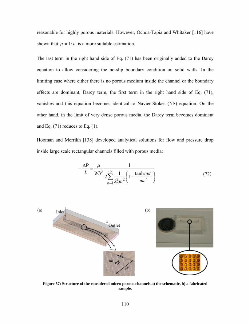
110
reasonable for highly porous materials. However, Ochoa-Tapia and Whitaker [116] have
shown that /1' is a more suitable estimation.
The last term in the right hand side of Eq. (71) has been originally added to the Darcy
equation to allow considering the no-slip boundary condition on solid walls. In the
limiting case where either there is no porous medium inside the channel or the boundary
effects are dominant, Darcy term, the first term in the right hand side of Eq. (71),
vanishes and this equation becomes identical to Navier-Stokes (NS) equation. On the
other hand, in the limit of very dense porous media, the Darcy term becomes dominant
and Eq. (71) reduces to Eq. (1).
Hooman and Merrikh [138] developed analytical solutions for flow and pressure drop
inside large scale rectangular channels filled with porous media:
122
3 tanh1
12
1
n n m
m
m
WhL
P
(72)
(a)
(b)
Figure 57: Structure of the considered micro-porous channels a) the schematic, b) a fabricated sample.

111
Where:
2/122,,2
12, Dam
K
hDa
n
W
hnn
(73)
and h , L and W are the depth, length, and width of the porous channel, respectively.
They also assumed that 1' . The cross-sectional aspect ratio, Wh / , in the
samples tested in the present study is smaller than 0.1. Therefore, instead of considering
the whole rectangular cross-section, the sample can be envisioned as a porous medium
sandwiched between two parallel plates as shown in Figure 58. The solution of Eq. (71),
the volume averaged velocity distribution, for 2D flow between parallel plates subject to
no-slip boundary condition on the channel walls becomes:
1
'sinh
'sinh
'sinh
K
h
K
hy
K
y
dx
dPKU
(74)
Consequently, the pressure drop for the simplified geometry becomes:
K
h
K
h
h
KhK
K
hQ
L
P
'sinh
'cosh1
'2
'sinh
(75)
To determine the pressure drop from Eq. (75), one needs to calculate the
permeability of the fibers arrangement in normal directions from the model developed in
Section 4.2, Eq. (51).

112
Figure 58: Schematic of the simplified 2D geometry.
4.2 Experimental procedure
4.2.1 Microfabrication
4.2.1.1 Soft lithography
Five different PDMS/PDMS samples were fabricated using the soft lithography
technique [139] described by Erickson et al. [140]. A schematic of the process is
provided in Figure 59. The fabrication process has two main parts: 1) preparing the mold;
2) making the PDMS replica.
SU-8 was used for preparing the molds; SU-8 is a negative tone epoxy-based
photoresist that can be photo patterned using deep UV light. SU-8-100 was chosen for
micromold fabrication as it can be patterned in very thick films (up to 1mm thick) and
can make an excellent mold for PDMS. Square glass slides of 75 x 75 mm and 1 mm thick
were used as substrates which were first cleaned in 100% Micro 90 Detergent (purchased
from International Products Corporation, USA) using ultrasonic agitation for 5 minutes
and then rinsed with de-ionized (DI) water, acetone, isopropyl alcohol (IPA) and DI
water. Substrates were blow dried using nitrogen followed by dehydration baking for 20
minutes at 120 °C in a convection oven and cooling to room temperature. A 25 nm thick
chrome layer was sputtered on each glass substrate which acts as an adhesion promoter
x y
U(h) = 0
U(0) = 0
h

113
for the SU-8 100. A 100 m thick layer of SU-8 100 was spin coated (at 2250 RPM) on
top of the adhesion layer of each substrate, followed by soft baking at 90 °C for 80
minutes and cooling to room temperature. Structures were patterned using
photolithographic UV exposure through a photomask for 60 seconds. Full crosslinking of
the SU-8 100 was achieved by a post-exposure bake at a temperature of 60°C for 65
minutes (ramp rate: 300 °C/hr) followed by cooling to room temperature. The structural
layer on each substrate was then developed in SU-8 Developer (Microchem™) for 90
seconds in an ultrasonic bath. Liquid PDMS was then poured over the mold and trapped
bubbles were extracted by placing the liquid PDMS inside a vacuum chamber for 1h. The
replica was then cured at 85°C for 45 minutes yielding a negative cast of the
microchannel pattern. An enclosed microchannel was then formed by bonding the PDMS
cast with another piece of PDMS via plasma treatment. The fabrication steps are depicted
in Figure 59.
As a result of the fabrication uncertainty, the sizes of the channels and the
cylinders were different from their intended dimensions. To measure the actual sizes, an
image processing technique, utilized by Akbari et al. [131], was used. Accuracy of this
method was reported by Akbari et al. [131] to be 3.6 m .
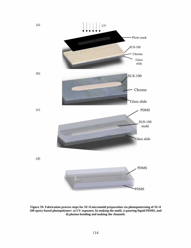
114
(a)
(b)
(c)
(d)
Figure 59: Fabrication process steps for SU-8 micromold preparation via photopatterning of SU-8 100 epoxy-based photopolymer: a) UV exposure, b) making the mold, c) pouring liquid PDMS, and
d) plasma bonding and making the channels.
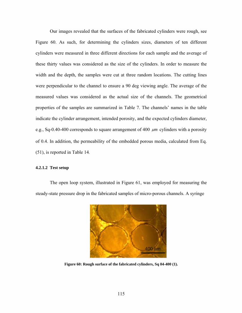
115
Our images revealed that the surfaces of the fabricated cylinders were rough, see
Figure 60. As such, for determining the cylinders sizes, diameters of ten different
cylinders were measured in three different directions for each sample and the average of
these thirty values was considered as the size of the cylinders. In order to measure the
width and the depth, the samples were cut at three random locations. The cutting lines
were perpendicular to the channel to ensure a 90 deg viewing angle. The average of the
measured values was considered as the actual size of the channels. The geometrical
properties of the samples are summarized in Table 7. The channels’ names in the table
indicate the cylinder arrangement, intended porosity, and the expected cylinders diameter,
e.g., Sq-0.40-400 corresponds to square arrangement of 400 m cylinders with a porosity
of 0.4. In addition, the permeability of the embedded porous media, calculated from Eq.
(51), is reported in Table 14.
4.2.1.2 Test setup
The open loop system, illustrated in Figure 61, was employed for measuring the
steady-state pressure drop in the fabricated samples of micro-porous channels. A syringe
Figure 60: Rough surface of the fabricated cylinders, Sq 04-400 (1).

116
Table 14: Geometrical properties of the fabricated samples.
Channel d ( m ) S ( m ) K ( 2m ), Eq. (51)
Sq-0.40-400 (1) 426 456 0.32 1.85×10⁻¹¹
Sq-0.40-400 (2) 418 456 0.34 3.30×10⁻¹¹
Sq-0.70-100 92 162 0.75 3.93×10⁻¹⁰
Sq-0.90-50 52 129 0.89 8.49×10⁻¹⁰
Sq-0.95-50 54 118 0.94 2.49×10⁻⁹
Channel W ( mm ) h ( m ) L ( cm )
Sq-0.40-400 (1) 3.18 96 1.46
Sq-0.40-400 (2) 3.19 105 1.46
Sq-0.70-100 1.45 105 1.72
Sq-0.90-50 1.27 129 2.00
Sq-0.95-50 1.70 118 2.22
pump (Harvard Apparatus, QC, Canada) fed the system with a controlled flow rate with
0.5% accuracy. Distilled water flowed through a submicron filter before entering the
channel.
To measure the pressure drop, a gauge pressure transducer (Omega Inc., Laval,
QC, Canada) was fixed at the channel inlet while the channel outlet was discharged to the
atmosphere. Teflon tubing (Scientific Products and Equipment, North York, Canada) was
employed to connect the pressure transducer to the syringe pump and the microchannel.
Pressure drops were measured for several flow rates in the range of 50-800 min/lit .

117
Figure 61: Schematic of the experimental setup for testing pressure drop in micro-porous channels.
4.2.1.3 Analysis of experimental data
Viscous dissipation effects are neglected in this study; thus, the properties of the
flowing water are considered to be constant. The measured pressure drop during the
experiment, totalP , is:
evFDDctotal PPPPPP minor
(76)
where cP is the pressure loss in the connecting tubes between the pressure transducer
and the sample inlet, see Figure 61, DP is the pressure drop in the developing region of
the samples where the fully-developed flow is not achieved, FDP is the pressure drop in
the regions with fully-developed velocity distribution. minorP is the pressure drop due
to minor losses in the samples including 90 deg bends in the inlet and outlet of the
samples, and evP is the pressure drop corresponding to the electroviscous effect [141].
Akbari et al. [131] showed that minorP and evP are less than 1% of the FDP and can
be neglected.
Syringe Pump
Pressure transducer
DAQ
SamplePC

118
The connecting pressure loss, cP , is measured directly at each flow rate when
the end of the tubing is disconnected from the sample. To perform accurate
measurements, the level of the tubing end should be identical to the case where the
samples are connected; this prevents any error due to hydrostatic pressure difference.
Akbari et al. [131] showed that the developing pressure drop in microchannels is less than
1% of the total pressure loss and is negligible. In addition, for the case of pack fibers,
fully-developed condition is achieved in the first three rows [63]. Therefore, it is expected
that the measured pressure drop in the sample is associated with the fully-developed
condition which is presented by Eq. (75).
The uncertainty of the analysis is mostly a result of the uncertainty in the
fabrication process and the uncertainty in the measurements. These uncertainties will
affect the porosity and consequently the permeability of the porous medium which is a
nonlinear function of porosity. The uncertainty in the permeability predictions can be
determined from the following relationship:
22
)()(
)()(
)(
)()(
dE
dd
KdE
d
KdKE
(77)
The uncertainty in the measurement of pressure drop can be evaluated from the following
equation:
2
222
)()(
)/(
)()(
)/()(
)(
)/()(
)(
)/(
)(
QEQd
LPd
KEKd
LPdhE
hd
LPdDaE
Dad
LPd
L
PE
(78)

119
Table 15: Uncertainty in the calculation of the involved parameters.
Sample )(E
K
KE )(
h
hE )(
)/(
)/(
LP
LPE
Sq-0.40-400 (1) 0.02 0.59 0.10 0.60
Sq-0.40-400 (2) 0.02 0.54 0.10 0.55
Sq-0.70-100 0.026 0.34 0.10 0.36
Sq-0.90-50 0.02 0.44 0.08 0.44
Sq-0.95-50 0.01 0.07 0.08 0.11
where:
22 )(
2
1)()(
K
KE
h
hE
Da
DaE
(79)
The associated uncertainty with different parameters involved in the analysis is
listed in Table 15. It can be seen that the overall uncertainty is significant; this is a direct
result of the nonlinear nature of the relationship between geometrical parameters with
permeability and the overall pressure drop. In the comparison of the experimental data
with the theoretical predictions only the trends should be considered.
4.2.2 Comparison of the model with the experimental data
Figure 62 and Figure 63 include the measured values of pressure drop in the
tested micro-porous channels versus the volumetric flow rate. The flow rates were
selected such that the pressure drop in the channels was higher than the accuracy of the
pressure transducer. It can be seen that the trends of the experimental data were well
predicted by the theoretical results, Eq. (75). The difference between most of the
measured data and the predicted values from Eq. (75) was less than %15. The deviations
were more intense for Sq-0.9-50 (max 20%); therefore, the 15% region for theoretical
120
predictions is shown in Figure 63. It should be noted the deviation of the experimental
data from the theoretical predictions is mostly caused by the inaccuracy in the channels
cross-section measurement as discussed before and the deviations are lower than the
uncertainty of the analysis.
The experimental values of pressure drop had a linear relationship with
volumetric flow rate. It can be argued that the channels had not been deformed during the
experiment else a nonlinear trend would have been observed in the experimental data; for
detailed discussions see [142]. Moreover, the linear trend of the experimental data shows
that the minor losses and the inertial effects are insignificant in the tested samples. It
should be noted that the maximum Reynolds number based on cylinders’ diameter is less
than 5; this justifies the observed trends in the measured values.
4.2.3 Numerical simulations
Our analysis showed a significant uncertainty in the experimental study.
Therefore, to further investigate the accuracy of the current analysis, the proposed
analytical model will be verified through comparison with independent numerical
simulations. Flow through 7 different geometries, listed in Table 16, is solved
numerically using Fluent. The geometrical parameters of the fist 5 samples are identical
to the fabricated channels. The geometry of the last 2 samples is selected such that a
wider range of porosity and permeability is covered.

121
Q (l/min)
P(P
a)
50 100 150 200 250 300 350
4000
8000
12000
16000Sq-0.4-400 (1), experimentSq-0.4-400 (2), experimentSq-0.7-100, experimentSq-0.4-400 (1), Eqs. (51),(75)Sq-0.4-400 (2), Eqs. (51),(75)Sq-0.7-100, Eqs. (51),(75)
Figure 62: Channel pressure drop versus flow rate for Sq-0.4-400 (1), Sq-0.4-400 (2), and Sq-0.7-100. Lines show the theoretical values of pressure drop predicted by Eq. (75) and symbols show the
experimental data.
Q (l/min)
P(P
a)
200 400 600 8000
2000
4000
6000Sq-0.9-50, experimentSq-0.95-50, experimentSq-0.9-50, Eqs. (51),(75)Sq-0.95-50, Eqs. (51),(75)Sq-0.9-50, Eqs. (51),(75)+15%Sq-0.9-50, Eqs. (51),(75) -15%
Figure 63: Channel pressure drop versus flow rate for Sq-0.9-50 and Sq-0.95-50. Lines show the theoretical values of pressure drop predicted by Eq. (75) and symbols show the experimental data.

122
Figure 64: The considered unit cell and produced numerical grid for modeling of sample Sq-04-400(2).
The flow is assumed to be fully-developed, creeping, and constant properties
(constant density and viscosity); therefore, modeling the region between two adjacent
cylinders and applying a periodic boundary condition enable us to estimate the pressure
gradient in the samples. An example of the considered geometry and the numerical grid
produced by Gambit [122] is shown in Figure 64.
The volumetric flow rate is set in the range covered by the experimental data to
ensure that the Reynolds number based on averaged velocity and the cylinders diameter is
low and the inertial effects are negligible. Fluent software [122] is used as the solver.
Second order upwind scheme is selected to discretize the governing equations. SIMPLE
algorithm is employed for pressure-velocity coupling. The inlet and outlet faces of the
geometry are considered to be Periodic. Symmetry boundary condition is applied at sides
of the considered unit cell. Grid parameters are varied to assess whether the predicted
pressure drops are independent of the computational grid.

123
Table 16: Geometrical parameters of the samples considered in the numerical simulations.
Channel d ( m ) S ( m ) W ( mm )
h ( m ) L ( cm )
Sq-0.40-400 (1) 426 456 0.32 3.18 96 1.46
Sq-0.40-400 (2) 418 456 0.34 3.19 105 1.46
Sq-0.40-400 (3) 400 450 0.4 3.15 100 1.5
Sq-0.50-400 400 500 0.5 3.0 100 1.5
Sq-0.70-100 92 162 0.75 1.45 105 1.72
Sq-0.90-50 52 129 0.89 1.27 129 2.00
Sq-0.95-50 54 118 0.94 1.70 118 2.22
In Figure 65 and Figure 66, the computed values of pressure drop for the tested
samples are compared with the model and the experimental data. It can be seen that Eq.
(75) can predict the trends of the experimental and numerical data; with the exception of
Sq-0.9-50 the deviations between the model and the data is less than 15%. However, the
difference between the numerical and the experimental results is due to the effects of the
geometrical uncertainty involved in the experiments.
4.2.4 Parametric study
In the present micro-porous channels, two parameters affect the pressure drop: 1)
the permeability, K ; 2) the channel depth, h . To investigate the effect of these
parameters, the dimensionless pressure drop is plotted versus the Darcy number in Figure
67. According to Nield and Kuznetsov [143] and Tamayol et al. [137], the hydrodynamic
boundary layer thickness scales with K . The Darcy number, Kh / , can be
interpreted as the ratio of the boundary layer thickness to the depth of the channel.

124
Q (l/min)
P(P
a)
50 100 150 200 250 300 3500
4000
8000
12000
16000
20000Sq-0.4-400 (1), experimentSq-0.4-400 (2), experimentSq-0.7-100, experimentSq-0.4-400 (1), theorySq-0.4-400 (2), theorySq-0.7-100, theorySq-0.4-400 (1), numericalSq-0.4-400 (2), numericalSq-0.7-400, numerical
Figure 65: Experimental, numerical, and theoretical values of channel pressure drop predicted by Eq. (75) versus flow rate for Sq-0.4-400 (1), Sq-0.4-400 (2), and Sq-0.7-100.
Q (l/min)
P(P
a)
200 400 600 8000
2000
4000
6000Sq-0.9-50, experimentSq-0.95-50, experimentSq-0.9-50, theorySq-0.95-50, theorySq-0.9-50, numericalSq-0.95-50, numerical
Figure 66: Experimental, numerical, and theoretical values of channel pressure drop predicted by Eq. (75) versus flow rate for Sq-0.9-50 and Sq-0.95-50.
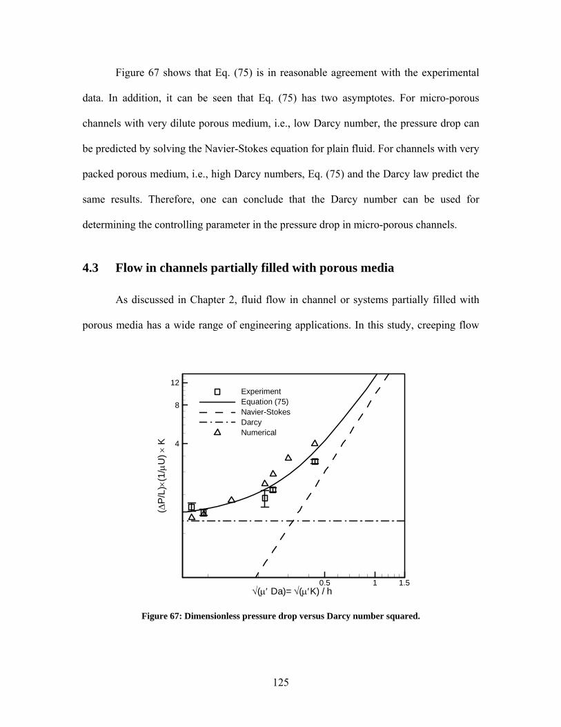
125
Figure 67 shows that Eq. (75) is in reasonable agreement with the experimental
data. In addition, it can be seen that Eq. (75) has two asymptotes. For micro-porous
channels with very dilute porous medium, i.e., low Darcy number, the pressure drop can
be predicted by solving the Navier-Stokes equation for plain fluid. For channels with very
packed porous medium, i.e., high Darcy numbers, Eq. (75) and the Darcy law predict the
same results. Therefore, one can conclude that the Darcy number can be used for
determining the controlling parameter in the pressure drop in micro-porous channels.
4.3 Flow in channels partially filled with porous media
As discussed in Chapter 2, fluid flow in channel or systems partially filled with
porous media has a wide range of engineering applications. In this study, creeping flow
( Da)= (K) / h
(P
/L)
(1/
U)
K
0.5 1 1.5
4
8
12ExperimentEquation (75)Navier-StokesDarcyNumerical
Figure 67: Dimensionless pressure drop versus Darcy number squared.

126
through mini/microchannels filled with regular arrays of cylinders, as shown in Figure
68, is investigated. Similar to the analysis of flow through channels fully filled with
porous media, the channel is considered to be wide enough such that the flow-field can be
modeled two dimensionally, as shown in Figure 68c. Moreover, flow is assumed to be
incompressible, constant properties, fully-developed, and creeping.
(a)
(b)
(c)
Figure 68: a) and b) Flow through channels partially filled with arrays of cylinders, c) simplified 2D geometry.
H
Region 2
Region 1
x
y
h

127
The domain can be divided into two regions. The upper region in Figure 68c only
contains the fluid phase; thus, the Stokes equation can be used:
y
dx
dP
y
u,
12
2
(80)
The applied boundary conditions in the region 1 are:
0)(,)( int Huuu
(81)
where intu is the interface velocity in the region 1. In the porous region (Region 2),
Brinkman equation is used for calculating the volume averaged velocity distribution:
y
dy
UdU
Kdx
dP DeffD ,
2
2
(82)
with the following boundary conditions:
int)(,0)0( DDD UUU
(83)
where intDU is the interface velocity in the porous region.
4.3.1 Solution development
The velocity distribution in the fluid region described by Eq. (80) subjected to
boundary conditions (81), is:
H
yHu
yHHyH
dx
dPu int
2
22 (84)
The solution of Eq. (82) with the boundary conditions of (83) is:

128
KyKyD eCeCK
dx
dPU '/
2'/
1
(85)
where:
KK
D
KK
K
ee
U
ee
eK
dx
dPC
'/'/int
'/'/
'/
21
(86)
21 CKdx
dPC
(87)
In Eqs. (84)-(87), intDU and intu remain unknown. These parameters can be found
through applying suitable conditions at the fluid porous interface. Various interface
boundary conditions proposed by researchers have been reviewed by Vafai and Alazmi
[117]. Moreover, they [117] showed that the overall effects of various interface
conditions on the velocity distribution are not significant. As such, the following
conditions are considered at the interface:
y
Deff
yD dy
dU
dy
duuU ),()(
(88)
which indicate the continuity of velocity and shear stress at the interface. Using Eqs.
(84)-(87) and the interface conditions of (88) the interface velocity is calculated as:
KK
KH
KHK
KKKH
dx
dp
uU D
'sinh'
'cosh'2
'sinh'
'cosh'2'2
intint
(89)

129
Having the velocity distribution, Eqs. (84)-(87) and (89) can be integrated over the entire
area, H , to calculate the pressure drop as a function of flow rate and the geometrical
properties of the channel and the porous medium. It is noteworthy that permeability
should be calculated from Eq. (51).
4.3.2 Comparison with experimental data
Arthur et al. [115], using a PIV technique, measured the velocity distribution
through a channel partially filled with porous media comprised of regular arrays of
cylinders. The reported values for velocity in the porous region are volume averaged
velocity. The properties of the tested samples are listed in Table 17. In Figure 69, the
reported velocity profile reported by Arthur et al. [115] is compared by the theoretical
calculations. It can be seen that the proposed solution can capture the observed trends in
the experimental results with a reasonable accuracy. Moreover, It can be seen that as the
porosity increases, i.e., the permeability increases, a larger volumetric flow rate passes
through the porous medium. For the case 1 with = 0.99, the velocity distribution is
very similar to an empty channel without porous medium and the effect of the porous
medium is not significant.
4.3.3 Numerical simulations
To investigate the accuracy of the current analysis, the proposed analytical model
will be verified through comparison with numerical simulations. Flow through 3 different
geometries, listed in Table 18, is solved numerically using Fluent. The flow is assumed to

130
Table 17: Geometrical parameters and averaged velocity for the samples tested by Arthur et al. [115].
Case d ( mm ) S ( mm ) H ( mm ) U ( smm / )
1 1.59 14.09 0.99 25 0.71
2 1.59 8.91 0.975 25 0.55
3 3.18 8.91 0.9 25 0.59
4 3.18 6.01 0.78 25 0.56
u / Uave
y/H
0 0.5 1 1.5 2 2.5 3 3.50
0.2
0.4
0.6
0.8
1
Experimental = 0.99Model = 0.99
Experimental = 0.975
Model = 0.975Experimental = 0.9
Model = 0.9
Experimental = 0.78Model = 0.78
Figure 69: Comparison of the velocity distribution reported by Arthur et al. [115] and the theoretical predictions by Eqs. (51) and (89).
be fully-developed, creeping, and constant properties; therefore, by applying a periodic
boundary condition, only flow through one row of cylinders is solved numerically. An
example of the considered geometry and the numerical grid produced by Gambit [122] is
shown in Figure 70.

131
Fluent software [122] is used as the solver. Second order upwind scheme is
selected to discretize the governing equations. SIMPLE algorithm is employed for
pressure-velocity coupling. The inlet and outlet faces of the geometry are considered to
be Periodic. A no slip boundary condition is applied at the solid surfaces including the
channel walls. Grid parameters are varied to test whether the predicted pressure drops are
independent of the computational grid.
(a)
(b)
Figure 70: a) The considered geometry and b) the produced numerical grid for modeling of sample with =0.4.
The volume averaged and the actual velocity distributions for porous media with
= 0.7 and 0.9 are compared in Figure 71 and Figure 72, respectively. The model can
accurately predict the average of the actual velocity profiles.
Table 18: Geometrical parameters considered in the numerical simulations.
Channel d ( m ) S ( m ) H ( mm ) ( mm ) K ( 2m )
1 100 114 0.99 1.7 1.25 6.62×10⁻⁸
2 100 162 0.975 2.4 1.75 2.79×10⁻⁶
3 100 280 0.9 4.2 3.0 3.52×10⁻⁵

132
u / Uave
y/H
0 1 2 3 4 50
0.2
0.4
0.6
0.8
1
= 0.7Model = 0.7 ' = 1
Figure 71: Comparison of the volume averaged (Eqs. (51) and (89)) and actual dimensionless velocity distributions in the channel filled with porous media with =0.7.
The computed velocity distributions for the three different cases are plotted in
Figure 73. It can be seen that as the porosity increases, i.e., the permeability increases, a
larger fraction of the flow passes through the porous medium. This is in agreement with
the observed trends in the experimental data reported by Arthur et al. [115]. Therefore,
for example for a typical fuel cell shown in Figure 4c where the GDL thickness is less
than 400 m , the in-plane permeability is approximately 211101 m , and the channel
height is 3 mm , less than 3% of flow passes through GDL. This result, confirms that gas
transport in the GDL is mostly diffusive rather than convective.

133
u / Uave
y/H
0 1 2 3 4 50
0.2
0.4
0.6
0.8
1
= 0.9
Model = 0.9, ' = 1
Figure 72: Comparison of the volume averaged (Eqs. (51) and (89))and actual dimensionless velocity distributions in the channel filled with porous media with =0.9.
u / Uave
y/H
0 1 2 3 4 50
0.2
0.4
0.6
0.8
1
= 0.4
= 0.7
= 0.9
Figure 73: Effects of porosity on the dimensionless microscopic velocity distribution through the channels partially filled with porous media.

134
5: CONCLUSIONS AND FUTURE WORK
The main focuses of this dissertation were on studying flow through systems that
include fibrous porous media and the resulting pressure drop both theoretically and
experimentally. The project was divided into two main parts: i) microscopic analysis and
ii) macroscopic modeling.
Flow properties of fibrous porous media including permeability and inertial
coefficient were investigated. Various techniques were employed to develop fundamental
understanding and models on the relationship between flow properties and salient
geometrical parameters. Moreover, three different testbeds were designed and built for
performing experiments to verify the theoretical analyses. The key contributions of the
present dissertation in this part can be summarized as follows:
1- An approximate but accurate model for flow distribution and permeability of
ordered arrays of fibers/cylinders was developed.
2- A novel scale analysis technique for permeability of 1D, 2D, and 3D fibrous
materials was proposed. The developed relationships were verified through
comparison with experimental data for a variety of materials measured during
this research or reported by others.
3- Mixing rules were successfully employed for predicting in-plane permeability
of complex, random microstructures.

135
4- Effects of compression and PTFE content on the permeability of GDLs were
measured. Moreover, the proposed model could capture the observed trends in
the experimental data.
5- Effects of salient microstructural properties specifically fiber orientation on
the pressure drop for moderate Reynolds number flows were investigated. The
results were used to develop correlations for inertial coefficient in the
investigated materials.
In the second part of the thesis, the developed models for permeability were
combined with volume-averaged equations to estimate volume-averaged velocity
distribution and pressure drop in confined porous media. The considered problems
were flow through channels fully or partially filled with fibrous media. The
highlights of my research in this part are:
1- In a novel analysis, the accuracy of the Brinkman equation in the micron-size
system was investigated.
2- Simple, closed-form analytical solutions for flow through channels partially
filled with porous media were developed and it was shown that this simple
analysis was accurate enough to be used in engineering analysis.
The outcomes of this dissertation provide new insights on the convective transport
in fibrous porous materials and are beneficial for designing related systems such as fuel
cells and compact heat exchangers.
136
5.1 Future plan
The following directions can be considered as the continuation of this dissertation:
1- Perform numerical simulations and experimental measurements on
fibrous materials with random microstructure. This should be used to
develop compact relationships for the inertial coefficient of the tested
materials.
2- Extend the analysis to convective heat transfer. Specially, the scale
analysis technique and the mixing rules have the potential to be used
for determining the interstitial heat transfer coefficient of complex
microstructures.
3- Investigate two phase flow through hydrophobic fibrous media such as
GDLs of PEMFCs or porous structures with pore size distribution in
the range of nano to micro millimeters. The water permeability
(apparent permeability) in these structures is different from the actual
permeability studied in this dissertation.
4- Conduct experiments on flow through various GDLs in the in-plane
and through-plane directions and including effects of microporous
layer in the analysis.
5- Test other regular and irregular arrays of microcylinders and also
random fibrous nanostructures to verify the analysis for microchannels
fully or partially filled with porous media for more cases.
137
6: REFERENCES
[1] M. Kaviany, Principles of Heat Transfer in Porous Media, 2nd ed., Springer-Verlag,
New York, 1995.
[2] L. Tadrist, M. Miscevic, O. Rahli, F. Topin, About the use of fibrous materials in
compact heat exchangers, Experimental Thermal and Fluid Science, 28(2-3) (2004) 193-
199.
[3] S. Mahjoob, K. .Vafai, A synthesis of fluid and thermal transport models for metal
foam heat exchangers, International Journal of Heat and Mass Transfer, 51(15-16) (2008)
3701-3711.
[4] G. A. Truskey, F. Yuan, D.E. Katz, Transport phenomena in biological systems,
Pearson Prentience Hall New Jersey, 2004.
[5] L. Spielman, S. L. Goren, Model for predicting pressure drop and filtration efficiency
in fibrous media, Current Research, 2 (1968) 279-287.
[6] M. A. Choi, M. H. Lee, J. Chang, S. J. Lee, Permeability modeling of fibrous media
in composite processing, Journal of Non-Newtonian Fluid Mechanics, 79(2-3) (1998)
585-598.
[7] C. Antoine, P. Nygård, O. W. Gregersen, R. Holmstad, T. Weitkamp, C. Rau, 3D
images of paper obtained by phase-contrast X-ray microtomography: image quality and
binarisation, Nuclear Instruments and Methods in Physics Research Section A:
138
Accelerators, Spectrometers, Detectors and Associated Equipment, 490(1-2) (2002) 392-
402.
[8] J. P. Feser, A. K. Prasad, S. G. Advani, Experimental characterization of in-plane
permeability of gas diffusion layers, Journal of Power Sources, 162(2) (2006) 1226-1231.
[9] J. T. Gostick, M. W. Fowler, M. D. Pritzker, M. A. Ioannidis, L.M. Behra, In-plane
and through-plane gas permeability of carbon fiber electrode backing layers, Journal of
Power Sources, 162(1) (2006) 228-238.
[10] F. Samani, M. Kokabi, M. Soleimani, M.R. V., Fabrication and characterization of
electrospun fibrous nanocomposite scaffolds based on poly(lactide-<I>co</I>-
glycolide)/poly(vinyl alcohol) blends, Polymer International, (2010).
[11] M. M. Tomadakis, T.J. Robertson, Viscous permeability of random fiber structures:
comparison of electrical and diffusional estimates with experimental and analytical
results, Journal of Composite Materials, 39(2) (2005) 163-188.
[12] A. Faghri, Z. Guo, Challenges and opportunities of thermal management issues
related to fuel cell technology and modeling, International Journal of Heat and Mass
Transfer, 48(19-20) (2005) 3891-3920.
[13] J. G. Pharoah, On the permeability of gas diffusion media used in PEM fuel cells,
Journal of Power Sources, 144(1) (2005) 77-82.
[14] T. V. Nguyen, A gas distributor design for proton-exchange-membrane fuel cells,
Journal of The Electrochemical Society, 143(5) (1996) L103-L105.

139
[15] B. T. Astrom, R. B. Pipes, S.G. Advani, On flow through aligned fiber beds and its
application to composites processing, Journal of Composite Materials, 26(9) (1992)
1351-1373.
[16] P.R. Waghmare, S.K. Mithra, A. Mather, J. McLaughlin, Modeling, fabrication and
simulation of microfilters, in: ECI International Conference on Heat Transfer and Fluid
Flow in Microscale, Whistler, Canada, 2008.
[17] C. Yu, M. H. Davey, F. Svec, J. M. J. Fréchet, Monolithic porous polymer for on-
chip solid-phase extraction and preconcentration prepared by photoinitiated in situ
polymerization within a microfluidic device, Analytical Chemistry, 73(21) (2001) 5088-
5096.
[18] D. J. Throckmorton, T. J. Shepodd, A. K. Singh, Electrochromatography in
microchips: reversed-phase separation of peptides and amino acids using photopatterned
rigid polymer monoliths, Analytical Chemistry, 74(4) (2002) 784-789.
[19] H. C. Brinkman, A calculation of the viscous force exerted by a flowing fluid on a
dense swarm of particles, Applied Scientific Research, 1(1) (1949) 27-34.
[20] F. A. L. Dullien, Porous media: fluid transport and pore structure, 2nd ed., Academic
Press, New York, 1992.
[21] J. Happel, H. Brenner, Low Reynolds number hydrodynamics: with special
applications to particulate media, 2nd ed., Martinus Nijhoff Publishers, The Hague, 1991.
[22] P.C. Carman, The determination of the specific surface of powders, Journal of the
Society of Chemical Industry, 57 (1938) 225-234.

140
[23] B. Markicevic, A. Bazylak, N. Djilali, Determination of transport parameters for
multiphase flow in porous gas diffusion electrodes using a capillary network model,
Journal of Power Sources, 171(2) (2007) 706-717.
[24] A. Bazylak, V. Berejnov, B. Markicevic, D. Sinton, N. Djilali, Numerical and
microfluidic pore networks: Towards designs for directed water transport in GDLs,
Electrochimica Acta, 53(26) (2008) 7630-7637.
[25] O. Chapuis, M. Prat, M. Quintard, E. Chane-Kane, O. Guillot, N. Mayer, Two-phase
flow and evaporation in model fibrous media: Application to the gas diffusion layer of
PEM fuel cells, Journal of Power Sources, 178(1) (2008) 258-268.
[26] P. K. Sinha, C. Y. Wang, Pore-network modeling of liquid water transport in gas
diffusion layer of a polymer electrolyte fuel cell, Electrochimica Acta, 52(28) (2007)
7936-7945.
[27] S. Kuwabara, The forces experienced by randomly distributed parallel circular
cylinders or spheres in a viscous flow at small Reynolds numbers, Journal of Physical
Society of Japan, 14 (1959) 527-532.
[28] J. Happel, Viscous flow relative to arrays of cylinders, AIChE Journal, 5(2) (1959)
174-177.
[29] H. Hasimoto, On the periodic fundamental solutions of the Stokes equations and
their application to viscous flow past a cubic array of spheres, Journal of Fluid Mechanics
5(02) (1959) 317-328.
[30] E. M. Sparrow, A. L. Loeffler, Longitudinal laminar flow between cylinders
arranged in regular array, AIChE Journal, 5 (1959) 325-330.

141
[31] A. S. Sangani , A. Acrivos, Slow flow past periodic arrays of cylinders with
application to heat transfer, International Journal of Multiphase Flow, 8(3) (1982) 193-
206.
[32] J. E. Drummond, M.I. Tahir, Laminar viscous flow through regular arrays of parallel
solid cylinders, International Journal of Multiphase Flow, 10(5) (1984) 515-540.
[33] J. B. Keller, Viscous flow through a grating or lattice of cylinders, Journal of Fluid
Mechanics 18 (1964) 94-96.
[34] B. R. Gebart, Permeability of Unidirectional Reinforcements for RTM, Journal of
Composite Materials, 26(8) (1992) 1100-1133.
[35] J. Van der Westhuizen, J. P. Du Plessis, An attempt to quantify fibre bed
permeability utilizing the phase average Navier-Stokes equation, Composites Part A:
Applied Science and Manufacturing, 27(4) (1996) 263-269.
[36] L. Skartsis, B. Khomami, J.L. Kardos, Resin flow through fiber beds during
composite manufacturing processes. Part II: Numerical and experimental studies of
newtonian flow through ideal and actual fiber beds, Polymer Engineering & Science,
32(4) (1992) 231-239.
[37] M. P. Sobera, C.R. Kleijn, Hydraulic permeability of ordered and disordered single-
layer arrays of cylinders, Physical Review E, 74(3) (2006) 036301.
[38] M. Sahraoui, M. Kaviany, Slip and no-slip velocity boundary conditions at interface
of porous, plain media, International Journal of Heat and Mass Transfer, 35(4) (1992)
927-943.

142
[39] A. S. Sangani, C. Yao, Transport processes in random arrays of cylinders. II.
Viscous flow, Physics of Fluids, 31(9) (1988) 2435-2444.
[40] J. J. L. Higdon, G.D. Ford, Permeability of three-dimensional models of fibrous
porous media, Journal of Fluid Mechanics 308(-1) (1996) 341-361.
[41] D. S. Clague, R. J. Phillips, A numerical calculation of the hydraulic permeability of
three-dimensional disordered fibrous media, Physics of Fluids, 9(6) (1997) 1562-1572.
[42] D. S. Clague, B. D. Kandhai, R. Zhang, P. M. A. Sloot, Hydraulic permeability of
(un)bounded fibrous media using the lattice Boltzmann method, Physical Review E,
61(1) (2000) 616-625.
[43] K. Boomsma, D. Poulikakos, Y. Ventikos, Simulations of flow through open cell
metal foams using an idealized periodic cell structure, International Journal of Heat and
Fluid Flow, 24(6) (2003) 825-834.
[44] M. Palassini, A. Remuzzi, Numerical analysis of viscous flow through fibrous
media: a model for glomerular basement membrane permeability, American Journal of
Physiology- Renal Physiology, 274(1) (1998) F223-231.
[45] T. Stylianopoulos, A. Yeckel, J. J. Derby, X. J. Luo, M. S. Shephard, E. A. Sander,
V. H. Barocas, Permeability calculations in three-dimensional isotropic and oriented fiber
networks, Physics of Fluids, 20(12) (2008) 123601.
[46] M. A. Tahir, H.V. Tafreshi, Influence of fiber orientation on the transverse
permeability of fibrous media, Physics of Fluids, 21(8) (2009) 083604.
143
[47] A. Koponen, D. Kandhai, E. Hellén, M. Alava, A. Hoekstra, M. Kataja, K.
Niskanen, P. Sloot, J. Timonen, Permeability of three-dimensional random fiber webs,
Physical Review Letters, 80(4) (1998) 716-719.
[48] S. Zobel, B. Maze, H. Vahedi Tafreshi, Q. Wang, B. Pourdeyhimi, Simulating
permeability of 3-D calendered fibrous structures, Chemical Engineering Science, 62(22)
(2007) 6285-6296.
[49] L. Hao, P. Cheng, Lattice Boltzmann simulations of anisotropic permeabilities in
carbon paper gas diffusion layers, Journal of Power Sources, 186(1) (2009) 104-114.
[50] A. Nabovati, E. W. Llewellin, A.C.M. Sousa, A general model for the permeability
of fibrous porous media based on fluid flow simulations using the lattice Boltzmann
method, Composites Part A: Applied Science and Manufacturing, 40(6-7) (2009) 860-
869.
[51] M. A. VanDoormaal, J.G. Pharoah, Determination of permeability in fibrous porous
media using the lattice Boltzmann method with application to PEM fuel cells,
International Journal for Numerical Methods in Fluids, 59(1) (2009) 75-89.
[52] G. Neale, W. Nader, Practical significance of brinkman's extension of darcy's law:
Coupled parallel flows within a channel and a bounding porous medium, The Canadian
Journal of Chemical Engineering, 52(4) (1974) 475-478.
[53] A. Tamayol, M. Bahrami, In-plane gas permeability of proton exchange membrane
fuel cell gas diffusion layers, Journal of Power Sources, 196(7) (2011) 3559-3564.
[54] G. W. Jackson, D.F. James, The permeability of fibrous porous media, The Canadian
Journal of Chemical Engineering, 64(3) (1986) 364-374.

144
[55] K. J. Mattern, W.M. Deen, Mixing rules for estimating the hydraulic permeability of
fiber mixtures, AIChE Journal, 54(1) (2008) 32-41.
[56] S. R. Eisenberg, A. J. Grodzinsky, Electrokinetic micromodel of extracellular matrix
and other polyelectrolyte networks, Physicochemical Hydrodynamics, 10 (1988) 517-
539.
[57] D. L. Johnson, J. Koplik, L. M. Schwartz, New pore-size parameter characterizing
transport in porous media, Physical Review Letters, 57(20) (1986) 2564-2567
[58] M. M. Tomadakis, S.V. Sotirchos, Transport properties of random arrays of freely
overlapping cylinders with various orientation distributions, The Journal of Chemical
Physics, 98(1) (1993) 616-626.
[59] E. J. Wiggins, W. B. Campbell, O. Mass, Determination of the Specific surface of
fibrous materials, The Canadian Journal of Research
17 (1939) 318-324.
[60] R. R. Sullivan, Specific surface measurements on compact bundles of parallel fibers,
Journal of Applied Physics, 13(11) (1942) 725-730.
[61] O. P. Bergelin, G. A. Brown, H. L. Hull, F. W. Sullivan, Heat transfer and fluid
friction during viscous flow across banks of tubes–III. A study of tube spacing and tube
size, ASME Transactions, 72 (1950) 881–888.
[62] C. N. Davies, The Separation of Airborne Dust and Particles, in: The Institution of
Mechanical Engineers, London, 1952, pp. 185–213.

145
[63] A. A. Kirsch, N.A. Fuchs, Studies on fibrous aerosol filters--II. pressure drops in
systems of parallel cylinders, Annals of Occupational Hygiene, 10(1) (1967) 23-30.
[64] A. G. Kostornov, M.S. Shevchuk, Hydraulic characteristics and structure of porous
metal fiber materials, Powder Metallurgy and Metal Ceramics, 16(9) (1977) 694-699.
[65] D. F. James, G. W. Jackson, The hydrodynamic resistance of hyaluronic acid and its
contribution to tissue permeability, Biorhelogy, 19 (1982) 317-330.
[66] T. G. Gutowski, Z. Cai, S. Bauer, D. Boucher, J. Kingery, S. Wineman,
Consolidation experiments for laminate composites, Journal of Composite Materials,
21(7) (1987) 650-669.
[67] C. Chmielewski, K. Jayaraman, The effect of polymer extensibility on crossflow of
polymer solutions through cylinder arrays, Journal of Rheology, 36(6) (1992) 1105-1126.
[68] B. Khomami, L.D. Moreno, Stability of viscoelastic flow around periodic arrays of
cylinders, Rheologica Acta, 36(4) (1997) 367-383.
[69] O. Rahli, L. Tadrist, M. Miscevic, R. Santini, Fluid flow through randomly packed
monodisperse fibers: The Kozeny-Carman parameter analysis, Journal of Fluids
Engineering, 119(1) (1997) 188-192.
[70] C. H. Shih, L.J. Lee, Effect of fiber architecture on permeability in liquid composite
molding, Polymer Composites, 19(5) (1998) 626-639.
[71] W. Zhong, I. Currie, D. James, Creeping flow through a model fibrous porous
medium, Experiments in Fluids, 40(1) (2006) 119-126.

146
[72] M. V. Williams, E. Begg, L. Bonville, H. R. Kunz, J.M. Fenton, Characterization of
gas diffusion layers for PEMFC, Journal of The Electrochemical Society, 151(8) (2004)
A1173-A1180.
[73] J. Ihonen, M. Mikkola, G. Lindbergh, Flooding of gas diffusion backing in PEFCs,
Journal of The Electrochemical Society, 151(8) (2004) A1152-A1161.
[74] B. Mueller, T. A. Zawodzinski, J. Bauman, F. Uribe, S. Gottesfeld, Carbon cloth
diffusion backings for high performance PEFC cathodes, in: T. F. Fuller, S. Gottesfeld
(Eds.) The Second International Symposium on Proton Conducting Membrane Fuel
Cells, 1999, pp. 1-9.
[75] M. Prasanna, H. Y. Ha, E. A. Cho, S. A. Hong, I.H. Oh, Influence of cathode gas
diffusion media on the performance of the PEMFCs, Journal of Power Sources, 131(1-2)
(2004) 147-154.
[76] M. F. Mathias, J. Roth, J. Fleming, W. Lehnert, Diffusion media materials and
characterization, in: W. Vielstich, H. A. Gasteiger, A. Lamm (Eds.) Handbook of Fuel
Cells—Fundamentals, Technology and Applications, John Wiley & Sons New York,
2003, pp. 517–537.
[77] L. Cindrella, A. M. Kannan, J. F. Lin, K. Saminathan, Y. Ho, C. W. Lin, J. Wertz,
Gas diffusion layer for proton exchange membrane fuel cells--A review, Journal of Power
Sources, 194(1) (2009) 146-160.
[78] W. A. Khan, J. R. Culham, M.M. Yovanovich, Convection heat transfer from tube
banks in crossflow: Analytical approach, International Journal of Heat and Mass
Transfer, 49(25-26) (2006) 4831-4838.

147
[79] D. Nagelhout, M. S. Bhat, J. C. Heinrich, D.R. Poirier, Permeability for flow normal
to a sparse array of fibres, Anglais, 191(1-2) (1995) 203-208.
[80] A. R. Martin, C. Saltiel, W. Shyy, Frictional losses and convective heat transfer in
sparse, periodic cylinder arrays in cross flow, International journal of heat and mass
transfer, 41(15) (1998) 2383-2397.
[81] S. L. Lee, J.H. Yang, Modeling of Darcy-Forchheimer drag for fluid flow across a
bank of circular cylinders, International journal of heat and mass transfer, 40(13) (1997)
3149-3155.
[82] D. L. Koch, A.J.C. Ladd, Moderate Reynolds number flows through periodic and
random arrays of aligned cylinders, Journal of Fluid Mechanics, 349(-1) (1997) 31-66.
[83] D. A. Edwards, M. Shapiro, P. Bar-Yoseph, M. Shapira, The influence of Reynolds
number upon the apparent permeability of spatially periodic arrays of cylinders, Physics
of Fluids A: Fluid Dynamics, 2(1) (1990) 45-55.
[84] C. K. Ghaddar, On the permeability of unidirectional fibrous media: A parallel
computational approach, Physics of Fluids, 7(11) (1995) 2563-2586.
[85] T. D. Papathanasiou, B. Markicevic, E.D. Dendy, A computational evaluation of the
Ergun and Forchheimer equations for fibrous porous media, Physics of Fluids, 13(10)
(2001) 2795-2804.
[86] X. Rong, G. He, D. Qi, Flows with inertia in a three-dimensional random fiber
network, Chemical Engineering Communications, 194 (2007) 398-406.

148
[87] F.P. Incropera, D.P. De Witt, Fundamentals of heat and mass transfer, 4th edition
ed., J. Wiley & Sons, 1996.
[88] O. P. Bergelin, G. A. Brown, S. C. Doberstein, Heat transfer and fluid friction during
flow across banks of tubes-IV: A study of the transition zone between viscous and
turbulent flow, ASME Journal of Heat Transfer, 74(953-959) (1952).
[89] M. L. Hunt, C.L. Tien, Effects of thermal dispersion on forced convection in fibrous
media, International Journal of Heat and Mass Transfer, 31(2) (1988) 301-309.
[90] V. V. Calmidi, R.L. Mahajan, Forced convection in high porosity metal foams,
Journal of Heat Transfer, 122(3) (2000) 557-565.
[91] K. Boomsma, D. Poulikakos, F. Zwick, Metal foams as compact high performance
heat exchangers, Mechanics of Materials, 35(12) (2003) 1161-1176.
[92] K. Boomsma, D. Poulikakos, The effects of compression and pore size variations on
the liquid flow characteristics in metal foams, Journal of Fluids Engineering, 124(1)
(2002) 263-272.
[93] J. J. Hwang, G. J. Hwang, R. H. Yeh, C.H. Chao, Measurement of interstitial
convective heat transfer and frictional drag for flow across metal foams, Journal of Heat
Transfer, 124(1) (2002) 120-129.
[94] A. Bhattacharya, V. V. Calmidi, R.L. Mahajan, Thermophysical properties of high
porosity metal foams, International Journal of Heat and Mass Transfer, 45(5) (2002)
1017-1031.

149
[95] S. Y. Kim, J. W. Paek, B. H. Kang, Thermal performance of aluminum-foam heat
sinks by forced air cooling, Components and Packaging Technologies, 26(1) (2003) 262-
267.
[96] P. Khayargoli, V. Loya, L. P. Lefebvre, M. Medraj, The impact of microstructure on
the permeability of metalfoams, in: CSME Forum 2004 2004, pp. 220-228.
[97] J. P. Bonnet, F. Topin, L. Tadrist, Flow laws in metal foams: compressibility and
pore size effects, Transport in Porous Media, 73(2) (2008) 233-254.
[98] N. Dukhan, Correlations for the pressure drop for flow through metal foam,
Experiments in Fluids, 41(4) (2006) 665-672.
[99] N. Dukhan, K. C. Chen, Heat transfer measurements in metal foam subjected to
constant heat flux, Experimental Thermal and Fluid Science, 32(2) (2007) 624-631.
[100] N. Dukhan, R. Picon-Feliciano, A. R. Alvarez-Hernandez, Air flow through
compressed and uncompressed aluminum foam: measurements and correlations, Journal
of Fluids Engineering, 128(5) (2006) 1004-1012.
[101] A. Haji-Sheikh, Fully developed heat transfer to fluid flow in rectangular passages
filled with porous materials, Journal of Heat Transfer, 128(6) (2006) 550-556.
[102] A. Haji-Sheikh, W. J. Minkowycz, E.M. Sparrow, Green's function solution of
temperature field for flow in porous passages, International Journal of Heat and Mass
Transfer, 47(22) (2004) 4685-4695.
[103] A. V. Kuznetsov, M. Xiong, D.A. Nield, Thermally developing forced convection
in a porous medium: circular duct with walls at constant temperature, with longitudinal

150
conduction and viscous dissipation effects, Transport in Porous Media, 53(3) (2003) 331-
345.
[104] K. Hooman A superposition approach to study slip-flow forced convection in
straight microchannels of uniform but arbitrary cross-section, International Journal of
Heat and Mass Transfer, 51(15-16) (2008) 3753-3762.
[105] K. Hooman, Slip flow forced convection in a microporous duct of rectangular
cross-section, Applied Thermal Engineering, 29(5-6) (2009) 1012-1019.
[106] A. Kosar, C. Mishra, Y. Peles, Laminar flow across a bank of low aspect ratio
micro pin fins, Journal of Fluids Engineering, 127(3) (2005) 419-430.
[107] S. Vanapalli, H. J. M. ter Brake, H. V. Jansen, J. F. Burger, H. J. Holland, T. T.
Veenstra, M.C. Elwenspoek, Pressure drop of laminar gas flows in a microchannel
containing various pillar matrices, Journal of Micromechanics and Microengineering,
17(7) (2007) 1381.
[108] J. Yeom, D. D. Agonafer, J. H. Han, M.A. Shannon, Low Reynolds number flow
across an array of cylindrical microposts in a microchannel and figure-of-merit analysis
of micropost-filled microreactors, Journal of Micromechanics and Microengineering,
19(6) (2009) 065025.
[109] G. S. Beavers, D. D. Joseph, Boundary conditions at a naturally permeable wall,
Journal of Fluid Mechanics, 30(01) (1967) 197-207.
[110] K. Vafai, S. J. Kim, On the limitations of the Brinkman-Forchheimer-extended
Darcy equation, International Journal of Heat and Fluid Flow, 16(1) (1995) 11-15.

151
[111] A. V. Kuznetsov, Analytical studies of forced convection in partly porous
configurations, in: K. Vafai (Ed.) Handbook of Porous Media, New York, 2000, pp. 269-
312.
[112] A. M. J. Davis, D. F. James, Penetration of shear flow into an array of rods aligned
with the flow, The Canadian Journal of Chemical Engineering, 82(6) (2004) 1169-1174.
[113] M. F. Tachie, D. F. James, I. G. Currie, Slow flow through a brush, Physics of
Fluids, 16(2) (2004) 445-451.
[114] M. Agelinchaab, M. F. Tachie, D. W. Ruth, Velocity measurement of flow through
a model three-dimensional porous medium, Physics of Fluids, 18(1) (2006) 017105.
[115] J. K. ARTHUR, D. W. RUTH, M. F. TACHIE, PIV measurements of flow through
a model porous medium with varying boundary conditions, Journal of Fluid Mechanics,
629 (2009) 343-374.
[116] J. A. Ochoa-Tapia, S. Whitaker, Momentum transfer at the boundary between a
porous medium and a homogeneous fluid--I. Theoretical development, International
Journal of Heat and Mass Transfer, 38(14) (1995) 2635-2646.
[117] B. Alazmi, K. Vafai, Analysis of fluid flow and heat transfer interfacial conditions
between a porous medium and a fluid layer, International Journal of Heat and Mass
Transfer, 44(9) (2001) 1735-1749.
[118] F. M. White, Fluid mechanics, 5th ed., McGraw-Hill Higher Education, 2003
152
[119] M. Bahrami, M. M. Yovanovich, J.R. Culham, Pressure drop of fully-developed,
laminar flow in microchannels of arbitrary cross-Section, Journal of Fluids Engineering,
128(5) (2006) 1036-1044.
[120] T. A. K. Sadiq, S. G. Advani, R.S. Parnas, Experimental investigation of transverse
flow through aligned cylinders, International Journal of Multiphase Flow, 21(5) (1995)
755-774.
[121] A. Tamayol, M. Bahrami, Analytical determination of viscous permeability of
fibrous porous media, International Journal of Heat and Mass Transfer, 52(9-10) (2009)
2407-2414.
[122] Fluent 6.3 User’s Guide, in, Fluent Inc., Lebanon, USA, 2007.
[123] H. K. Versteeg, W. Malalasekera, An introduction to computational fluid dynamics,
Longman Scientific and Technical, Essex, UK, 1995.
[124] A. Tamayol, M. Bahrami, Laminar flow in microchannels with noncircular cross
section, Journal of Fluids Engineering, 132(11) (2010) 111201.
[125] F.S. Shit, Laminar flow in axisymmetric conduits by a rational approach, The
Canadian Journal of Chemical Engineering, 45(5) (1967) 285-294.
[126] A. Tamayol, M. Bahrami, Laminar flow in microchannels with noncircular cross
section, Journal of Fluids Engineering, 132(11) (2010) 111201.
[127] D. A. Nield, A. Bejan, Convection in porous media, 2nd ed., Springer-Verlag, New
York, 1999.

153
[128] B. P. Boudreau, The diffusive tortuosity of fine-grained unlithified sediments,
Geochimica et Cosmochimica Acta, 60(16) (1996) 3139-3142.
[129] L. Shen, Z. Chen, Critical review of the impact of tortuosity on diffusion, Chemical
Engineering Science, 62(14) (2007) 3748-3755.
[130] G. E. Archie, The Electrical Resistivity Log as an Aid in Determining Some
Reservoir Characteristics Transactions of AIME, 146 (1942) 54-62.
[131] M. Akbari, D. Sinton, M. Bahrami, Pressure drop in rectangular microchannels as
compared with theory based on arbitrary cross section, Journal of Fluids Engineering,
131(4) (2009) 041202-041201-041208.
[132] J. A. Molnar, L. Trevino, L. J. Lee, Liquid flow in molds with percolated fiber
mats, Polymer Composites, 10(6) (1989) 414–423.
[133] J. R. Taylor, An introduction to error analysis: The study of uncertainties in
physical measurements, Second ed., University Science Books,, Sausalito, USA, 1997.
[134] A. Z. Weber, J. Newman, Modeling transport in polymer-electrolyte fuel cells,
Chemical Reviews, 104(10) (2004) 4679-4726.
[135] A. Tamayol, M. Bahrami, Transverse permeability of fibrous porous media
Physical Review E, In Press (2011).
[136] R. C. Givler, S.A. Altobelli, A determination of the effective viscosity for the
Brinkman–Forchheimer flow model, Journal of Fluid Mechanics 258(1) (1994) 355-370.

154
[137] A. Tamayol, K. Hooman, M. Bahrami, Thermal analysis of flow in a porous
medium over a permeable stretching wall, Transport in Porous Media, 85(3) (2010) 661-
676.
[138] K. Hooman, A. A. Merrikh, Analytical solution of forced convection in a duct of
rectangular cross section saturated by a porous medium, Journal of Heat Transfer, 128(6)
(2006) 596-600.
[139] J. C. McDonald, D. C. Duffy, J. R. Anderson, D. T. Chiu, H. Wu, O. J. A.
Schueller, G.M. Whitesides, Fabrication of microfluidic systems in
poly(dimethylsiloxane), Electrophoresis, 21(1) (2000) 27-40.
[140] D. Erickson, D. Sinton, D. Li, Joule heating and heat transfer in
poly(dimethylsiloxane) microfluidic systems, Lab on a Chip, 3 (2003) 141-149.
[141] R.F. Probstein, Physicochemical hydrodynamics: An introduction, 2nd ed., John
Wiley & Sons Inc., New York, 1994.
[142] M. A. Holden, S. Kumar, A. Beskok, P. S. Cremer, Microfluidic diffusion diluter:
bulging of PDMS Microchannels under pressure driven flow, Journal of Micromechanics
and Microengineering, 13 (2003) 412–418.
[143] D.A. Nield, A.V. Kuznetsov, Forced convection in porous media: transverse
heterogeneity effects and thermal development, in: K. Vafai (Ed.) Handbook of Porous
Media, Taylor and Francis,, New York,, 2005, pp. 143-193.
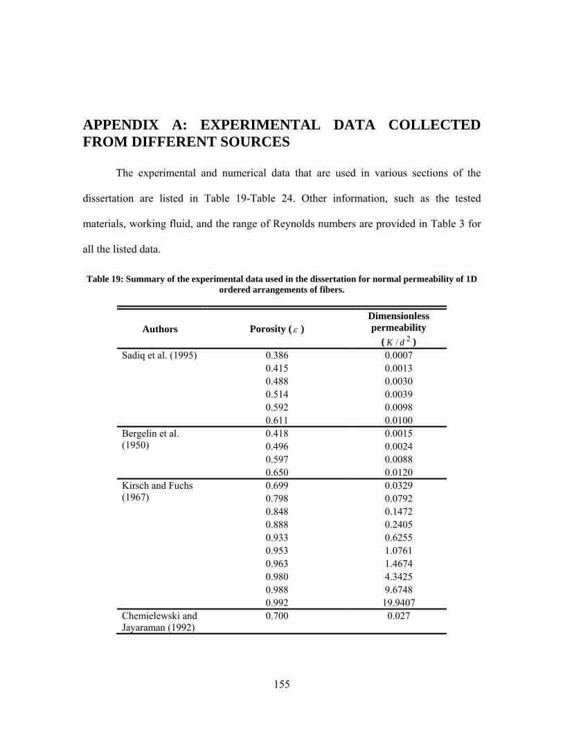
155
APPENDIX A: EXPERIMENTAL DATA COLLECTED FROM DIFFERENT SOURCES
The experimental and numerical data that are used in various sections of the
dissertation are listed in Table 19-Table 24. Other information, such as the tested
materials, working fluid, and the range of Reynolds numbers are provided in Table 3 for
all the listed data.
Table 19: Summary of the experimental data used in the dissertation for normal permeability of 1D ordered arrangements of fibers.
Authors Porosity ( ) Dimensionless permeability
( 2/ dK ) Sadiq et al. (1995) 0.386 0.0007
0.415 0.0013 0.488 0.0030 0.514 0.0039 0.592 0.0098 0.611 0.0100
Bergelin et al. (1950)
0.418 0.0015 0.496 0.0024 0.597 0.0088 0.650 0.0120
Kirsch and Fuchs (1967)
0.699 0.0329 0.798 0.0792 0.848 0.1472 0.888 0.2405 0.933 0.6255 0.953 1.0761 0.963 1.4674 0.980 4.3425 0.988 9.6748 0.992 19.9407
Chemielewski and Jayaraman (1992)
0.700 0.027
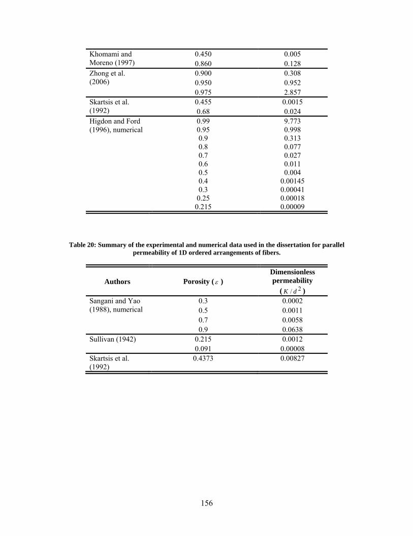
156
Khomami and Moreno (1997)
0.450 0.005 0.860 0.128
Zhong et al. (2006)
0.900 0.308 0.950 0.952 0.975 2.857
Skartsis et al. (1992)
0.455 0.0015 0.68 0.024
Higdon and Ford (1996), numerical
0.99 9.773 0.95 0.998 0.9 0.313 0.8 0.077 0.7 0.027 0.6 0.011 0.5 0.004 0.4 0.00145 0.3 0.00041
0.25 0.00018 0.215 0.00009
Table 20: Summary of the experimental and numerical data used in the dissertation for parallel permeability of 1D ordered arrangements of fibers.
Authors Porosity ( ) Dimensionless permeability
( 2/ dK ) Sangani and Yao (1988), numerical
0.3 0.0002 0.5 0.0011 0.7 0.0058 0.9 0.0638
Sullivan (1942) 0.215 0.0012 0.091 0.00008
Skartsis et al. (1992)
0.4373 0.00827
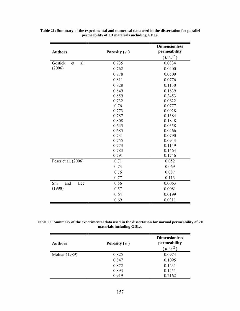
157
Table 21: Summary of the experimental and numerical data used in the dissertation for parallel permeability of 2D materials including GDLs.
Authors Porosity ( ) Dimensionless permeability
( 2/ dK ) Gostick et al. (2006)
0.735 0.0334 0.762 0.0400 0.778 0.0509 0.811 0.0776 0.828 0.1130 0.849 0.1839
0.859 0.2453 0.732 0.0622 0.76 0.0777 0.773 0.0928 0.787 0.1384 0.808 0.1848 0.645 0.0358 0.685 0.0466 0.731 0.0790 0.755 0.0943 0.773 0.1149 0.783 0.1464 0.791 0.1746 Feser et al. (2006) 0.71 0.052
0.73 0.069 0.76 0.087 0.77 0.113
Shi and Lee (1998)
0.56 0.0063 0.57 0.0081 0.64 0.0199 0.69 0.0311
Table 22: Summary of the experimental data used in the dissertation for normal permeability of 2D materials including GDLs.
Authors Porosity ( ) Dimensionless permeability
( 2/ dK ) Molnar (1989) 0.825 0.0974
0.847 0.1095 0.872 0.1231
0.893 0.1451 0.919 0.2162

158
Authors Porosity ( ) Dimensionless permeability
( 2/ dK ) Davies (1952) 0.779 0.0654
0.808 0.1021 0.83 0.1321 0.85 0.1750
0.87 0.2162 0.88 0.1835 0.90 0.3375 0.90 0.4168 0.90 0.5269 0.91 0.4686 0.91 0.3454 0.92 0.5394 0.92 0.6209 0.92 0.5394 Gostick et al. (2006)
0.88 0.423 0.81 0.216 0.84 0.268
0.85 0.110 0.8 0.102 Zobel et al. (2007) 0.965 0.666
0.962 0.586 0.918 0.189
0.898 0.123 0.893 0.225 0.872 0.097 0.849 0.115 Kostornov and Shevchuck (1967)
0.29 0.00004 0.36 0.00035 0.49 0.00150 0.59 0.00538 0.69 0.01428 0.29 0.00019 0.36 0.00054 0.49 0.00210 0.59 0.00705
0.69 0.01925 0.29 0.00004

159
Table 23: Summary of the experimental and numerical data used in the dissertation for normal permeability of 3D materials with the exception of metalfoams.
Authors Porosity ( ) Dimensionless permeability
( 2/ dK ) Carman (1937) 0.681 0.035
0.688 0.040 0.722 0.0585
0.731 0.0613 0.757 0.0805 0.765 0.09475 Rahli et al. (1997) 0.600 0.013
0.640 0.022 0.700 0.041
0.739 0.081 0.769 0.119 0.800 0.163 0.840 0.345 0.851 0.409 0.890 0.864 Jackson and James (1982)
0.9896 18.75 0.99379 29.25 0.99586 51 0.99724 66.75
0.99793 77 0.99862 125 0.99931 332.5 Rahli et al. (1996) 0.388 0.00083
0.462 0.00259 0.525 0.00440 0.599 0.013
0.643 0.021 0.697 0.041 0.739 0.079 0.773 0.124 0.804 0.164 0.847 0.342 0.896 0.803 Higdon and Ford (1996), numerical
0.9856 9.681 0.9784 5.566 0.9179 0.7414
0.8762 0.3639 0.8272 0.1933 0.7739 0.1027 0.7163 0.0591 0.653 0.0339 0.5882 0.0195

160
Authors Porosity ( ) Dimensionless permeability
( 2/ dK ) 0.4571 0.0059 0.3318 0.0016 0.2166 0.00029
Table 24: Summary of the experimental and numerical data used in the dissertation for permeability of metalfoams.
Authors Porosity ( ) PPI Ligament
diameter ( d )
Pore diameter
( pd )
Permeability ( K )
Khayargoli et al. (2004)
0.9 11.16 N.A. 1.40×10⁻³ 2.76×10⁻⁸ 0.89 17.23 N.A. 9.00×10⁻⁴ 1.55×10⁻⁸ 0.9 27.33 N.A. 6.00×10⁻⁴ 4.87×10⁻⁹
0.83 37.43 N.A. 5.00×10⁻⁴ 3.39×10⁻⁹ 0.86 47.53 N.A. 4.00×10⁻⁴ 1.77×10⁻⁹ 0.9 11.16 N.A. 1.40×10⁻³ 2.76×10⁻⁸ Boomsma and Poulikakos (2002)
0.921 10 N.A. 0.0069 3.53×10⁻⁷ 0.92 20 N.A. 0.0036 1.09×10⁻⁷ 0.928 40 N.A. 0.0023 7.12×10⁻⁸ 0.921 10 N.A. 0.0069 3.53×10⁻⁷
Dukhan (2006) 0.919 10 0.000439 0.002057 1×10⁻⁷ 0.915 10 0.000443 0.002053 8×10⁻⁸
0.919 20 0.000222 0.001037 6.3×10⁻⁸ 0.924 20 0.00022 0.00104 5.4×10⁻⁸ Bhattacharya et al. (2002)
0.9726 5 0.0005 0.00402 2.70×10⁻⁷ 0.9118 5 0.00055 0.0038 1.80×10⁻⁷ 0.9486 10 0.0004 0.00313 1.20×10⁻⁷
0.9138 10 0.00045 0.00328 1.10×10⁻⁷ 0.8991 10 0.00043 0.0032 9.40E-08 0.9546 20 0.0003 0.0027 1.30×10⁻⁷ 0.9245 20 0.00035 0.0029 1.10×10⁻⁷ 0.9005 20 0.00035 0.00258 9.00×10⁻⁸ 0.9659 40 0.0002 0.0019 5.00×10⁻⁸ 0.9272 40 0.00025 0.00202 6.10×10⁻⁸ 0.9132 40 0.0002 0.0018 5.30×10⁻⁸ 0.971 5 0.00051 0.004 2.52×10⁻⁷ 0.946 5 0.00047 0.0039 2.17×10⁻⁷ 0.905 5 0.00049 0.0038 1.74×10⁻⁷ 0.949 10 0.00037 0.0031 1.49×10⁻⁷ 0.909 10 0.00038 0.00296 1.11×10⁻⁷ 0.978 20 0.00038 0.0028 1.42×10⁻⁷ 0.949 20 0.00032 0.0027 1.19×10⁻⁷
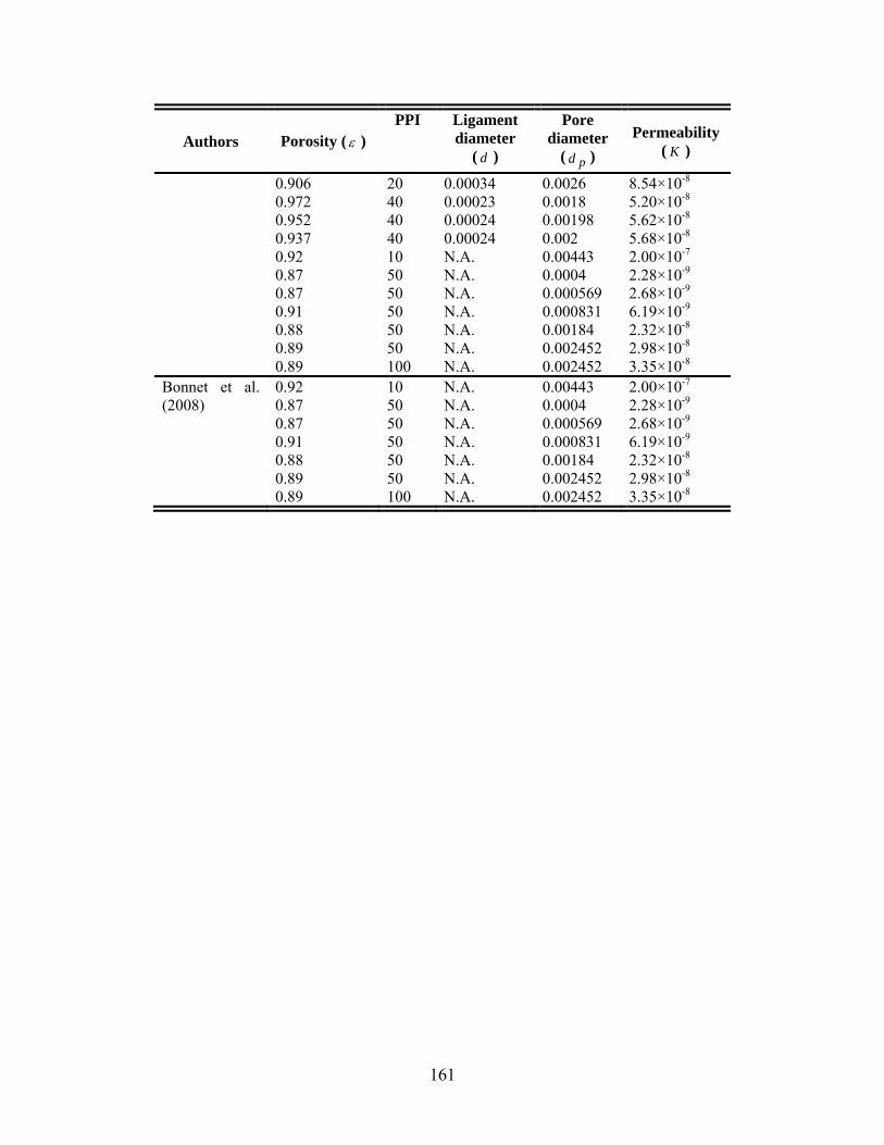
161
Authors Porosity ( ) PPI Ligament
diameter ( d )
Pore diameter
( pd )
Permeability ( K )
0.906 20 0.00034 0.0026 8.54×10⁻⁸ 0.972 40 0.00023 0.0018 5.20×10⁻⁸ 0.952 40 0.00024 0.00198 5.62×10⁻⁸ 0.937 40 0.00024 0.002 5.68×10⁻⁸ 0.92 10 N.A. 0.00443 2.00×10⁻⁷ 0.87 50 N.A. 0.0004 2.28×10⁻⁹ 0.87 50 N.A. 0.000569 2.68×10⁻⁹ 0.91 50 N.A. 0.000831 6.19×10⁻⁹ 0.88 50 N.A. 0.00184 2.32×10⁻⁸ 0.89 50 N.A. 0.002452 2.98×10⁻⁸ 0.89 100 N.A. 0.002452 3.35×10⁻⁸ Bonnet et al. (2008)
0.92 10 N.A. 0.00443 2.00×10⁻⁷ 0.87 50 N.A. 0.0004 2.28×10⁻⁹
0.87 50 N.A. 0.000569 2.68×10⁻⁹ 0.91 50 N.A. 0.000831 6.19×10⁻⁹ 0.88 50 N.A. 0.00184 2.32×10⁻⁸ 0.89 50 N.A. 0.002452 2.98×10⁻⁸ 0.89 100 N.A. 0.002452 3.35×10⁻⁸

162
APPENDIX B: DETAILS OF THE EXPERIMENTAL MEASUREMENTS CARRIED OUT IN THE DISSERTATION
Details of the experimental measurements for calculating flow properties of the
investigated materials, described in Sections 3.5, 3.6, and 3.7, are listed in this appendix.
In Table 25-Table 27 data from different trials for measuring properties of similar
samples are also included. The analysis of uncertainty associated with each experiment is
available in the designated section in the text.
Table 25: Summary of the measurements and calculations for determining permeability of tube banks and metalfoams; pure glycerol with viscosity of 1.4 is used as working fluid.
Porosity ( )
Fiber diameter
(mm)
Flow rate (lps×10-7)
Length* (mm)
Pressure drop (Pa)
Reynolds number
Permeability (K×10-7)
Tube bank 0.8 1.5 2.7 59 243.5 0.00065 1.3 0.8 1.5 65 59 601.2 0.00158 1.2 0.8 1.5 57 59 523.8 0.00138 1.2 0.8 1.5 16 59 144.7 0.00040 1.3 0.8 1.5 4.9 59 42.0 0.00012 1.3 0.8 1.5 13 59 121.9 0.00032 1.3 0.8 1.5 38 59 337.1 0.00091 1.3 0.8 1.5 6.3 52 47.1 0.00016 1.2 0.8 1.5 57 52 460.8 0.00139 1.1 0.8 1.5 32 52 251.4 0.00079 1.2 0.8 1.5 21 52 158.9 0.00051 1.2 0.8 1.5 13 52 101.1 0.00033 1.2
0.85 1.5 1.87 52 56.8 0.0005 3.42 0.85 1.5 2.89 52 90.0 0.0007 3.33 0.85 1.5 9.12 52 281.0 0.0023 3.37 0.85 1.5 5.04 52 155.1 0.0013 3.37 0.85 1.5 10.91 52 330.9 0.0027 3.42

163
Porosity ( )
Fiber diameter
(mm)
Flow rate (lps×10-7)
Length* (mm)
Pressure drop (Pa)
Reynolds number
Permeability (K×10-7)
0.85 1.5 12.95 52 397.4 0.0032 3.38 0.85 1.5 2.94 52 89.5 0.0007 3.41 0.85 1.5 7.40 52 222.6 0.0018 3.45 0.85 1.5 1.34 52 40.6 0.0003 3.42 0.85 1.5 4.56 52 136.6 0.0011 3.46 0.85 1.5 5.27 52 156.5 0.0013 3.50 0.85 1.5 2.27 52 67.7 0.0006 3.48 0.85 1.5 12.13 52 361.3 0.0030 3.48 0.9 1.5 4.68 80 135.6 0.0012 5.55 0.9 1.5 3.3 80 92.9 0.0008 5.73 0.9 1.5 12 80 356.5 0.0030 5.42 0.9 1.5 14.4 80 434.0 0.0036 5.36 0.9 1.5 20.3 80 620.2 0.0051 5.27 0.9 1.5 2.25 80 62.5 0.0006 5.79 0.9 1.5 5.67 80 171.7 0.0014 5.32 0.9 1.5 3.53 52 70.6 0.0009 3.33 0.9 1.5 1.12 52 21.5 0.0003 3.48 0.9 1.5 5.58 52 111.9 0.0014 3.32 0.9 1.5 8.70 52 153.6 0.0021 3.77 0.9 1.5 17.50 52 323.5 0.0043 3.60 0.9 1.5 10.97 52 201.5 0.0027 3.63
Metalfoams 0.929 (10)‡ 0.41 9.60 52 443.9 0.00075 2.51
0.929 0.41 2.73 52 126.7 0.00021 2.50 0.929 0.41 0.82 52 30.8 0.00006 3.08 0.929 0.41 2.51 52 116.5 0.00020 2.50 0.929 0.41 5.36 52 260.8 0.00042 2.38 0.929 0.41 14.80 52 712.3 0.00116 2.41 0.929 0.41 1.95 52 84.0 0.00015 2.69 0.929 0.41 7.59 52 333.5 0.00059 2.64 0.929 0.41 7.65 52 357.7 0.00060 2.48
0.929 (10) 0.41 2.12 52 87.1 0.00017 2.71 0.929 0.41 10.56 52 527.5 0.00084 2.68 0.929 0.41 3.30 52 131.9 0.00026 2.78 0.929 0.41 7.53 52 304.3 0.00060 2.75
0.934 (20) 0.3 2.38 52 195.0 0.00013 1.48 0.934 0.3 4.17 52 363.7 0.00024 1.39 0.934 0.3 1.65 52 136.6 0.00009 1.46 0.934 0.3 0.70 52 54.9 0.00004 1.55 0.934 0.3 2.92 52 248.2 0.00017 1.43 0.934 0.3 4.88 52 421.6 0.00028 1.40 0.934 0.3 2.49 52 209.3 0.00014 1.44 0.934 0.3 7.80 52 632.1 0.00044 1.50
0.934 (20) 0.3 3.28 52 228.7 0.00020 1.61 0.934 0.3 9.42 52 668.6 0.00057 1.58

164
Porosity ( )
Fiber diameter
(mm)
Flow rate (lps×10-7)
Length* (mm)
Pressure drop (Pa)
Reynolds number
Permeability (K×10-7)
0.934 0.3 1.34 52 81.0 0.00008 1.86 0.934 0.3 5.09 52 341.8 0.00031 1.68 0.934 0.3 2.35 52 150.4 0.00014 1.76 0.934 0.3 2.93 52 249.2 0.00018 1.32
0.942 (40) 0.2 2.79 52 115.2 0.00037 0.84 0.942 0.2 2.75 52 112.4 0.00036 0.85 0.942 0.2 9.74 52 455.3 0.00129 0.74 0.942 0.2 9.08 52 422.1 0.00120 0.74 0.942 0.2 3.82 52 151.3 0.00050 0.87 0.942 0.2 6.51 52 291.4 0.00086 0.77 0.942 0.2 11.73 52 543.2 0.00155 0.75 0.942 0.2 12.47 52 555.1 0.00165 0.78
0.942 (40) 0.2 0.81 52 417.3 0.00011 0.81 0.942 0.2 0.81 52 412.6 0.00010 0.81 0.942 0.2 0.82 52 562.2 0.00014 0.82 0.942 0.2 0.80 52 745.1 0.00019 0.80 0.942 0.2 0.81 52 236.8 0.00006 0.81
* The distance between pressure taps.
‡ The number in the parentheses shows the PPI in metalfoam samples.
Table 26: Summary of the measurements and calculations for determining the permeability of GDLs; samples diameter is 0.0254 m.
Initial thickness
( m )
Thickness ( m ) Porosity ( )
PTFE (%)
Pressure drop (Pa)
Flow rate
(lpm)
Permeability ( K )
Toray TGP 120
380 380 0.8 0 28.6 1.5 1.30×10⁻¹¹ 380 380 0.8 0 46.8 2 1.06×10⁻¹¹ 380 380 0.8 0 69.0 3 1.08×10⁻¹¹ 380 380 0.8 0 96.9 4 1.02×10⁻¹¹ 380 380 0.8 0 128.3 5 9.64×10⁻¹² 380 380 0.8 0 157.9 6 9.40×10⁻¹² 368 368 0.8 0 35.9 1.5 1.00×10⁻¹¹ 368 368 0.8 0 45.8 2 1.05×10⁻¹¹ 368 368 0.8 0 66.3 3 1.09×10⁻¹¹ 368 368 0.8 0 87.4 4 1.10×10⁻¹¹ 368 368 0.8 0 114.8 5 1.04×10⁻¹¹ 377 350 0.78 0 30.6 1.5 1.12×10⁻¹¹ 377 350 0.78 0 47.6 2 9.58×10⁻¹² 377 350 0.78 0 69.0 3 9.91×10⁻¹² 377 350 0.78 0 97.7 4 9.33×10⁻¹²

165
Initial thickness
( m )
Thickness ( m ) Porosity ( )
PTFE (%)
Pressure drop (Pa)
Flow rate
(lpm)
Permeability ( K )
377 350 0.78 0 132.1 5 8.63×10⁻¹² 377 350 0.78 0 173.9 6 7.86×10⁻¹² 374 325 0.76 0 39.6 1.5 8.02×10⁻¹² 374 325 0.76 0 50.0 2 8.46×10⁻¹² 374 325 0.76 0 83.2 3 7.63×10⁻¹² 374 325 0.76 0 111.8 4 7.57×10⁻¹² 374 325 0.76 0 159.7 5 6.63×10⁻¹² 379 285 0.73 0 49.6 1.5 5.61×10⁻¹² 379 285 0.73 0 66.3 2 5.60×10⁻¹² 379 285 0.73 0 102.7 3 5.42×10⁻¹² 379 285 0.73 0 144.3 4 5.14×10⁻¹² 379 285 0.73 0 204.1 5 4.55×10⁻¹² 372 272 0.72 0 56.3 1.5 4.72×10⁻¹² 372 272 0.72 0 77.2 2 4.59×10⁻¹² 372 272 0.72 0 117.6 3 4.52×10⁻¹² 372 272 0.72 0 164.7 4 4.30×10⁻¹² 364 364 0.79 10 36.4 1.5 9.77×10⁻¹² 364 364 0.79 10 47.3 2 1.00×10⁻¹¹ 364 364 0.79 10 72.0 3 9.88×10⁻¹² 364 364 0.79 10 93.7 4 1.01×10⁻¹¹ 364 364 0.79 10 121.3 5 9.77×10⁻¹² 364 364 0.79 10 150.3 6 9.47×10⁻¹² 365 365 0.79 10 33.9 1.5 1.05×10⁻¹¹ 365 365 0.79 10 46.1 2 1.03×10⁻¹¹ 365 365 0.79 10 68.5 3 1.04×10⁻¹¹ 365 365 0.79 10 94.7 4 1.00×10⁻¹¹ 365 365 0.79 10 128.1 5 9.28×10⁻¹² 365 365 0.79 10 160.7 6 8.87×10⁻¹² 365 365 0.77 20 35.7 1.5 1.00×10⁻¹¹ 365 365 0.77 20 45.0 2 1.06×10⁻¹¹ 365 365 0.77 20 76.4 3 9.33×10⁻¹² 365 365 0.77 20 108.1 4 8.80×10⁻¹² 365 365 0.77 20 148.9 5 7.98×10⁻¹² 365 365 0.77 20 203.0 6 7.03×10⁻¹² 371 371 0.77 20 36.9 1.5 9.80×10⁻¹² 371 371 0.77 20 50.3 2 9.57×10⁻¹² 371 371 0.77 20 74.0 3 9.77×10⁻¹² 371 371 0.77 20 108.9 4 8.85×10⁻¹² 371 371 0.77 20 141.8 5 8.50×10⁻¹² 347 347 0.76 30 54.1 1.5 6.27×10⁻¹² 347 347 0.76 30 76.5 2 5.91×10⁻¹² 347 347 0.76 30 121.1 3 5.60×10⁻¹² 347 347 0.76 30 53.3 1.5 6.36×10⁻¹² 347 347 0.76 30 78.7 2 5.74×10⁻¹²

166
Initial thickness
( m )
Thickness ( m ) Porosity ( )
PTFE (%)
Pressure drop (Pa)
Flow rate
(lpm)
Permeability ( K )
Toray TGP 90
267 267 0.8 0 21.6 1.5 1.02×10⁻¹¹ 267 267 0.8 0 31.0 2 9.22×10⁻¹² 267 267 0.8 0 46.2 3 8.71×10⁻¹² 267 267 0.8 0 63.4 4 8.45×10⁻¹² 267 267 0.8 0 86.7 5 7.76×10⁻¹² 254 240 0.8 0 113.6 6 7.45×10⁻¹² 254 240 0.79 0 30.6 1.5 1.09×10⁻¹¹ 254 240 0.79 0 39.5 2 1.01×10⁻¹¹ 254 240 0.79 0 64.1 3 1.01×10⁻¹¹ 254 240 0.79 0 83.0 4 9.86×10⁻¹² 254 240 0.79 0 114.7 5 9.02×10⁻¹² 254 240 0.79 0 154.5 6 8.26×10⁻¹² 260 228 0.77 0 30.6 1.5 7.27×10⁻¹² 260 228 0.77 0 39.5 2 7.51×10⁻¹² 260 228 0.77 0 64.1 3 6.95×10⁻¹² 260 228 0.77 0 83.0 4 7.15×10⁻¹² 260 228 0.77 0 114.7 5 6.47×10⁻¹² 260 228 0.77 0 154.5 6 5.77×10⁻¹² 267 207 0.74 0 31.7 1.5 6.38×10⁻¹² 267 207 0.74 0 44.8 2 6.02×10⁻¹² 267 207 0.74 0 71.2 3 5.68×10⁻¹² 267 207 0.74 0 99.4 4 5.43×10⁻¹² 267 207 0.74 0 142.3 5 4.74×10⁻¹² 267 207 0.74 0 192.6 6 4.20×10⁻¹² 255 200 0.74 0 34.6 1.5 5.65×10⁻¹² 255 200 0.74 0 52.0 2 5.01×10⁻¹² 255 200 0.74 0 77.4 3 5.05×10⁻¹² 255 200 0.74 0 107.8 4 4.83×10⁻¹² 255 200 0.74 0 149.0 5 4.37×10⁻¹² 255 200 0.74 0 209.5 6 3.73×10⁻¹²
Sigracet SGL 10AA
414 414 0.88 0 9.1 1.5 4.46×10⁻¹¹ 414 414 0.88 0 13.3 2 4.05×10⁻¹¹ 414 414 0.88 0 22.2 3 3.65×10⁻¹¹ 414 414 0.88 0 32.3 4 3.33×10⁻¹¹ 414 414 0.88 0 47.8 5 2.82×10⁻¹¹ 414 414 0.88 0 64.3 6 2.51×10⁻¹¹ 385 290 0.84 0 11.2 1.5 2.53×10⁻¹¹ 385 290 0.84 0 16.0 2 2.36×10⁻¹¹ 385 290 0.84 0 25.5 3 2.22×10⁻¹¹ 385 290 0.84 0 37.9 4 1.99×10⁻¹¹ 385 290 0.84 0 55.0 5 1.72×10⁻¹¹ 385 290 0.84 0 76.6 6 1.48×10⁻¹¹
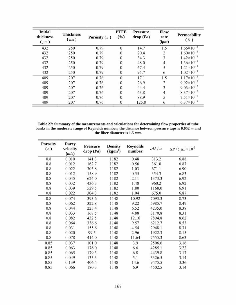
167
Initial thickness
( m )
Thickness ( m ) Porosity ( )
PTFE (%)
Pressure drop (Pa)
Flow rate
(lpm)
Permeability ( K )
432 250 0.79 0 14.7 1.5 1.66×10⁻¹¹ 432 250 0.79 0 20.4 2 1.60×10⁻¹¹ 432 250 0.79 0 34.3 3 1.42×10⁻¹¹ 432 250 0.79 0 48.0 4 1.36×10⁻¹¹ 432 250 0.79 0 67.4 5 1.21×10⁻¹¹ 432 250 0.79 0 95.7 6 1.02×10⁻¹¹ 409 207 0.76 0 17.1 1.5 1.17×10⁻¹¹ 409 207 0.76 0 26.9 2 9.92×10⁻¹² 409 207 0.76 0 44.4 3 9.03×10⁻¹² 409 207 0.76 0 63.8 4 8.37×10⁻¹² 409 207 0.76 0 88.9 5 7.51×10⁻¹² 409 207 0.76 0 125.8 6 6.37×10⁻¹²
Table 27: Summary of the measurements and calculations for determining flow properties of tube banks in the moderate range of Reynolds number; the distance between pressure taps is 0.052 m and
the fiber diameter is 1.5 mm.
Porosity ( )
Darcy velocity
(m/s)
Pressure drop (Pa)
Density (kg/m3)
Reynolds number
/U 610/ LUP
0.8 0.010 141.3 1182 0.48 313.2 6.88 0.8 0.012 162.7 1182 0.56 361.0 6.87 0.8 0.022 303.8 1182 1.03 671.1 6.90 0.8 0.012 158.9 1182 0.55 354.3 6.83 0.8 0.045 624.0 1182 2.11 1373.3 6.92 0.8 0.032 436.3 1182 1.48 960.2 6.92 0.8 0.039 529.5 1182 1.80 1168.0 6.91 0.8 0.022 304.3 1182 1.04 675.0 6.87 0.8 0.074 393.6 1148 10.92 7093.3 8.73 0.8 0.062 322.8 1148 9.22 5985.7 8.49 0.8 0.044 225.4 1148 6.52 4235.0 8.38 0.8 0.033 167.5 1148 4.88 3170.8 8.31 0.8 0.082 432.5 1148 12.16 7894.8 8.62 0.8 0.064 336.6 1148 9.57 6212.7 8.53 0.8 0.031 155.6 1148 4.54 2948.1 8.31 0.8 0.020 99.5 1148 2.96 1922.3 8.15 0.8 0.078 414.0 1148 11.64 7555.3 8.63
0.85 0.037 101.0 1148 3.9 2506.6 3.16 0.85 0.063 176.0 1148 6.6 4285.1 3.22 0.85 0.065 179.3 1148 6.8 4439.8 3.17 0.85 0.049 133.3 1148 5.1 3326.5 3.14 0.85 0.139 406.4 1148 14.6 9475.5 3.36 0.85 0.066 180.3 1148 6.9 4502.5 3.14

168
Porosity ( )
Darcy velocity
(m/s)
Pressure drop (Pa)
Density (kg/m3)
Reynolds number
/U 610/ LUP
0.85 0.077 218.8 1148 8.1 5247.2 3.27 0.85 0.098 283.4 1148 10.3 6687.2 3.32 0.85 0.018 82.4 1182 1.1 682.0 2.68 0.85 0.052 236.8 1182 3.0 1924.5 2.73 0.85 0.069 324.7 1182 3.9 2549.9 2.83 0.85 0.017 80.0 1182 1.0 629.5 2.82 0.85 0.038 172.7 1182 2.2 1413.1 2.71 0.85 0.095 459.1 1182 5.4 3509.0 2.90 0.85 0.054 243.9 1182 3.0 1977.3 2.74 0.85 0.078 354.6 1182 4.4 2887.1 2.73 0.90 0.036 119.5 1182 1.8 1138.0 1.78 0.90 0.061 208.4 1182 3.0 1945.4 1.81 0.90 0.063 212.3 1182 3.1 2015.7 1.78 0.90 0.047 157.8 1182 2.3 1510.2 1.77 0.90 0.135 469.9 1182 6.6 4301.8 1.85 0.90 0.064 213.5 1182 3.1 2044.1 1.76 0.90 0.075 259.0 1182 3.7 2382.2 1.84 0.90 0.095 329.9 1182 4.7 3036.0 1.84 0.90 0.035 60.1 1148 3.9 2560.1 2.08 0.90 0.053 88.1 1148 5.9 3841.6 2.03 0.90 0.080 144.2 1148 8.9 5796.5 2.20 0.90 0.067 119.0 1148 7.5 4843.9 2.18 0.90 0.100 175.1 1148 11.2 7253.8 2.14 0.90 0.047 79.1 1148 5.2 3405.9 2.06 0.90 0.063 106.7 1148 7.0 4536.0 2.08 0.90 0.085 148.9 1148 9.5 6162.6 2.14

169
APPENDIX C: DETAILS OF THE NUMERICAL SIMULATIONS PERFORMED IN THE DISSERTATION
Numerical simulations are used in various parts of this dissertation to verify the
developed theoretical models/solutions. In this appendix, more details on the numerical
results and calculations are provided. Numerical grid generation and then computations
for all the studied cases are carried out using Gambit and Fluent software, respectively.
Flow normal to ordered array of cylinders (Sections 3.2 and 3.7):
Although fully-developed solution for normal flow can be found by simulating a single
unit cell and applying periodic boundary condition, to determine the developing length
for flow in the medium, as was shown in Figure 16a, a set of 7-10 unit cells in series are
considered and velocity profiles are compared at the entrance to each unit cell, see Figure
74. The pressure drops used for calculation of permeability are the values obtained from
the regions with fully-developed flow.
The inlet velocity of the media is assumed to be uniform. Constant pressure boundary
condition is applied at the computational domain outlet. The symmetry boundary
condition is applied on the side borders of the considered unit cells; this means that
normal velocity and gradient of parallel component of the velocity on the side borders are
zero.
In Figure 74, the comparison of the entrance and exit velocity profile to the fourth (out of
10) unit cell with = 0.9 indicates that fully developed condition is achieved after the

170
third row of cylinders. It should be noted that in the unit cell with = 0.9, the distance
between the fibers is larger than other cases; thus, has the longest developing length. As
such, it is expected that a similar trend holds for the rest of the studied cases, i.e., the fully
developed condition is achieved after the third row of cylinders.
y/S
u/U
D
0 0.25 0.5 0.75 10
1
2
3
4
5
6
7
8
9
10
Numerical, x/S=0Numerical x/S=1.0
Figure 74: Developed velocity profiles in the inlet and outlet of the fourth unit cell with =0.9.
Independence of the results from numerical grid size is tested for different cases and the
size of computational grid used for each geometry is selected such that the maximum
difference in the predicted values for pressure gradient to be less than 2%. For example,
Figure 75 illustrates the independency of the calculated values of pressure drop over a
unit cell with = 0.9 after a computational grid size of 16000. Moreover, as shown in
Figure 76, the numerical results are in reasonable agreement with experimental and
numerical data reported by other; this also confirms the accuracy of the analysis. The
summary of the calculated results is presented in Table 28. Therefore, a grid size of

171
15,000 – 20,000 is used through the analysis for predicting the flow properties of ordered
arrays of cylinders.
Grid size
P(P
a)
0 25000 50000 75000 100000
2
4
Figure 75: The pressure drop over a unit cell with =0.9 calculated with different number of grids.
+
+
+
K* =
K/d
2
0.4 0.6 0.8 110-4
10-3
10-2
10-1
100
101
102
Berglin et al. (1950)Kirsch and Fuchs (1967)Sadiq et al. (1995)Khomami and Moreno (1997)Zhong et al. (2006)Present numerical results
+
Figure 76: Comparison between the present numerical results and experimental data, normal flow through square arrays of cylinders.
d
y
x S
Flow
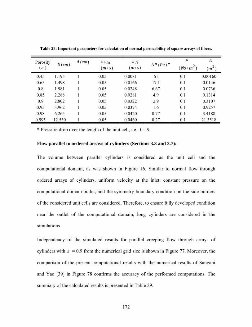
172
Table 28: Important parameters for calculation of normal permeability of square arrays of fibers.
Porosity ( )
)(cmS )(cmd
inletu
)/( sm DU
)/( sm )(PaP *
)/( 2mNs
K
)( 2m
0.45 1.195 1 0.05 0.0081 61 0.1 0.00160 0.65 1.498 1 0.05 0.0166 17.1 0.1 0.0146 0.8 1.981 1 0.05 0.0248 6.67 0.1 0.0736
0.85 2.288 1 0.05 0.0281 4.9 0.1 0.1314 0.9 2.802 1 0.05 0.0322 2.9 0.1 0.3107
0.95 3.962 1 0.05 0.0374 1.6 0.1 0.9257 0.98 6.265 1 0.05 0.0420 0.77 0.1 3.4188
0.995 12.530 1 0.05 0.0460 0.27 0.1 21.3518
* Pressure drop over the length of the unit cell, i.e., L= S.
Flow parallel to ordered arrays of cylinders (Sections 3.3 and 3.7):
The volume between parallel cylinders is considered as the unit cell and the
computational domain, as was shown in Figure 16. Similar to normal flow through
ordered arrays of cylinders, uniform velocity at the inlet, constant pressure on the
computational domain outlet, and the symmetry boundary condition on the side borders
of the considered unit cells are considered. Therefore, to ensure fully developed condition
near the outlet of the computational domain, long cylinders are considered in the
simulations.
Independency of the simulated results for parallel creeping flow through arrays of
cylinders with = 0.9 from the numerical grid size is shown in Figure 77. Moreover, the
comparison of the present computational results with the numerical results of Sangani
and Yao [39] in Figure 78 confirms the accuracy of the performed computations. The
summary of the calculated results is presented in Table 29.

173
Grid size
P(P
a)
0 50000 100000 1500000
2
4
Figure 77: The pressure drop over a length of 2cm for square arrays of cylinders with d= 1 cm and =0.9 calculated with different number of grids.
K* =
K/d
2
0.2 0.3 0.4 0.5 0.6 0.7 0.8 0.910-4
10-3
10-2
10-1
100
101
102
Sullivan (1942)Skartsis et al. (1992)Sangani and Yao (1988)Present numerical results
Figure 78: Comparison between the present numerical results, experimental data, and the numerical results of Sangani and Yao [39] for parallel permeability of square arrays of cylinders.
d
S
S
Flow
y
x

174
Table 29: The numerical results of parallel permeability in square arrays of fibers, cmd 1 and
smuinlet /05.0 .
)(cmS )(cm )/( smUD )(PaP *K0.215 1 5 0.01075 404.3 0.0013 0.35 1.10 5 0.0175 228.7 0.0038 0.45 1.19 2 0.0225 56.8 0.0079 0.55 1.32 5 0.0275 77.6 0.0177 0.65 1.50 5 0.0325 43 0.0378 0.8 1.98 5 0.04 12 0.1667 0.9 2.80 2 0.045 1.33 0.6712
Flow parallel and normal to ordered 2D and 3D arrays of cylinders (Section 3.7):
Navier-Stokes equations are solved numerically using Fluent [122]. The second order
upwind scheme is selected to discretize the governing equations and SIMPLE algorithm
[123] is employed for pressure-velocity coupling. For simple cubic structures, the inlet
and outlet boundaries of the computational domains are considered to be periodic, i.e., the
velocity distributions on both boundaries are the same. The symmetry boundary condition
is applied on the side borders of the considered unit cells; this means that normal velocity
and gradient of parallel component of the velocity on the side borders are zero. However,
for 3 dimensional cases, employing the periodic condition leads to a poor convergence
rate. As a result of our limited computational resources, following our results for 1D
structures, a set of 7-10 unit cells in series is considered and velocity profiles are
compared at the entrance to each unit cell for modeling flow normal and parallel to 2D
structures. For these cases, the inlet velocity of the media is assumed to be uniform.
Constant pressure boundary condition is applied on the computational domain outlet. The
pressure drops used for calculation of flow properties are only the values obtained from

175
the developed regions. Typical computational grids used in the analysis are shown in
Figure 79.
In spite of the complexity of the computational domain, our analysis showed that the
number of computational grids used in the analysis does not significantly affect the
numerical flow-field. For example, in Figure 80, the plotted pressure drops per unit
length in 3D structures calculated by two different grids confirm that grid size has a
negligible effect on the numerical results over a wide range of Reynolds numbers. This is
mainly a result of laminar nature of flow-field without turbulent and major recirculation
regions. In addition, the very good agreement of the predicted values of permeability for
SC structures with the results reported by Higdon and Ford [40], shown in Figure 54,
justifies the accuracy of the present computations.
Details of the numerical results used for calculating the inertial coefficient in 1D, 2D, and
3D structures are presented in Table 30.

176
Figure 79: Typical computational domain used for modeling of flow a) through simple cubic; b) parallel to 2D; c) transverse to 2D fibrous structures.

177
Grid size
P/L
(Pa/
m)
0 150000 300000 4500000
20
40
60
80
100
120
140
Re = 3Re = 30
Figure 80: The pressure drop over a unit cell of simple cubic arrays of cylinders with d= 1 cm and S = 4 cm for two different Reynolds numbers, calculated with different number of grids.
Table 30: Summary of the measurements and calculation for calculating flow properties of fibrous structures in the moderate range of Reynolds number; the fiber diameter is 10 mm.
Porosity ( )
Darcy velocity
(m/s)
Pressure drop (Pa)
Length (m)
Density (kg/m3)
Reynolds number
/U 610/ LUP
Normal flow, 1D structures 0.45 0.0001 0.066 0.012 100 0.008 0.8 6.81 0.45 0.0008 0.662 0.012 100 0.081 8.1 6.80 0.45 0.0081 6.700 0.012 100 0.815 81.5 6.88 0.45 0.0815 68.130 0.012 100 8.148 814.8 7.00 0.45 0.8148 965.950 0.012 100 81.48 8148.0 9.92 0.65 0.0002 0.017 0.015 100 0.02 1.7 0.68 0.65 0.0017 0.172 0.015 100 0.17 16.6 0.69 0.65 0.0166 1.72 0.015 100 1.66 166.1 0.69 0.65 0.1661 18.49 0.015 100 16.6 1661 0.74 0.65 0.3323 40.0 0.015 100 33.2 3323 0.80 0.65 0.6645 87.3 0.015 100 66.4 6645 0.88 0.65 1.6614 264.1 0.015 100 166.1 16613 1.1 0.8 0.0002 0.007 0.0198 100 0.02 2.5 0.137 0.8 0.0025 0.067 0.0198 100 0.25 24.8 0.137 0.8 0.0248 0.677 0.0198 100 2.48 247.6 0.138 0.8 0.2476 7.9 0.0198 100 24.76 2476.2 0.161 0.8 0.9905 40.3 0.0198 100 99.05 9904.9 0.206 0.8 1.4857 70.9 0.0198 100 148.57 14857.4 0.241

178
Porosity ( )
Darcy velocity
(m/s)
Pressure drop (Pa)
Length (m)
Density (kg/m3)
Reynolds number
/U 610/ LUP
0.8 2.4762 142.4 0.0198 100 247.62 24762.3 0.29 0.9 0.0003 0.003 0.028 100 0.03 3.2 0.033 0.9 0.0032 0.030 0.028 100 0.32 32.2 0.033 0.9 0.0322 0.299 0.028 100 3.22 321.5 0.033 0.9 0.3215 3.43 0.028 100 32.15 3215.4 0.038 0.9 1.2862 20.51 0.028 100 128.62 12861.7 0.057 0.9 1.9293 37.90 0.028 100 192.93 19292.5 0.070
0.95 0.0004 0.0017 0.04 100 0.04 3.7 0.011 0.95 0.0037 0.0165 0.04 100 0.37 37.4 0.011 0.95 0.0374 0.168 0.04 100 3.74 373.8 0.013 0.95 0.3738 2.19 0.04 100 37.38 3738.1 0.015 0.95 0.7476 5.65 0.04 100 74.76 7476.2 0.019
Transverse flow through 2D structures 0.35 0.00009 0.13 0.01 100 0.01 0.9 14.5 0.35 0.00862 12.54 0.01 100 0.9 86.2 14.5 0.35 0.08620 127.53 0.01 100 8.6 862.0 14.8 0.35 0.34479 638.74 0.01 100 34.5 3447.9 18.5 0.5 0.0002 0.04 0.01 100 0.02 1.8 2.17 0.5 0.0182 3.96 0.01 100 1.82 181.7 2.18 0.5 0.1817 44.50 0.01 100 18.17 1816.9 2.45 0.5 0.3634 101.49 0.01 100 36.34 3633.8 2.79 0.6 0.0002 0.0207 0.01 100 0.02 2.5 0.84 0.6 0.025 2.076 0.01 100 2.45 245.4 0.85 0.6 0.245 25.56 0.01 100 24.54 2453.5 1.04 0.6 0.491 61.2 0.01 100 49.07 4907.0 1.25 0.8 0.0004 0.0035 0.01 100 0.04 3.7 0.094 0.8 0.0373 0.364 0.01 100 3.73 372.7 0.097 0.8 0.1491 1.611 0.01 100 14.91 1490.7 0.108 0.8 0.3727 5.046 0.01 100 37.27 3726.8 0.135 0.8 0.5963 9.205 0.01 100 59.63 5962.8 0.154
Parallel flow through 2D structures 0.5 0.000125 0.028 0.015708 100 0.012 1.25 1.43 0.5 0.0125 2.832 0.015708 100 1.25 125 1.44 0.5 0.125 30.54 0.015708 100 12.5 1250 1.56 0.5 0.5 138.2 0.015708 100 50 5000 1.76 0.6 0.00015 0.018 0.0196 100 0.015 1.5 0.61 0.6 0.015 1.8 0.0196 100 1.5 150 0.61 0.6 0.15 19.38 0.0196 100 15 1500 0.66 0.6 0.3 41.05 0.0196 100 30 3000 0.70 0.8 0.02 10.21 0.03927 10 0.02 2 0.130 0.8 0.0002 0.00973 0.03927 100 0.02 2 0.124 0.8 0.2 11.98 0.03927 100 20 2000 0.153 0.8 0.12 7.07 0.03927 100 12 1200 0.150 0.8 0.8 60.45 0.03927 100 80 8000 0.192 0.9 0.000225 0.00425 0.07854 100 0.0225 2.25 0.0241
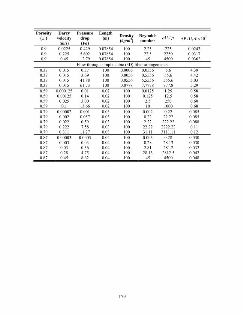
179
Porosity ( )
Darcy velocity
(m/s)
Pressure drop (Pa)
Length (m)
Density (kg/m3)
Reynolds number
/U 610/ LUP
0.9 0.0225 0.429 0.07854 100 2.25 225 0.0243 0.9 0.225 5.602 0.07854 100 22.5 2250 0.0317 0.9 0.45 12.79 0.07854 100 45 4500 0.0362
Flow through simple cubic (3D) fiber arrangements 0.37 0.015 0.37 100 0.0006 0.0556 5.6 4.39 0.37 0.015 3.69 100 0.0056 0.5556 55.6 4.42 0.37 0.015 41.88 100 0.0556 5.5556 555.6 5.03 0.37 0.015 61.73 100 0.0778 7.7778 777.8 5.29 0.59 0.000125 0.01 0.02 100 0.0125 1.25 0.58 0.59 0.00125 0.14 0.02 100 0.125 12.5 0.58 0.59 0.025 3.00 0.02 100 2.5 250 0.60 0.59 0.1 13.66 0.02 100 10 1000 0.68 0.79 0.00002 0.001 0.03 100 0.002 0.22 0.085 0.79 0.002 0.057 0.03 100 0.22 22.22 0.085 0.79 0.022 0.59 0.03 100 2.22 222.22 0.088 0.79 0.222 7.58 0.03 100 22.22 2222.22 0.11 0.79 0.311 11.27 0.03 100 31.11 3111.11 0.12 0.87 0.00003 0.0003 0.04 100 0.003 0.28 0.030 0.87 0.003 0.03 0.04 100 0.28 28.13 0.030 0.87 0.03 0.36 0.04 100 2.81 281.2 0.032 0.87 0.28 4.75 0.04 100 28.13 2812.5 0.042 0.87 0.45 8.62 0.04 100 45 4500 0.048