Embed Size (px)
Citation preview

Microeconomics of Reliable Urban Water Supply
The Comparative Economic Advantage of
Great Lakes Cities
by:
William L. Holahan
Department of Economics
University of Wisconsin‐Milwaukee
Center for Economic Development
Working Paper
May 2010

2
ABSTRACT
This paper presents some of the elements of microeconomics that are valuable in formulating water policy in older cities along the Great Lakes. In their heydays these cities installed capacity in anticipation of greater economic activity than they now have. Now they face decisions on water pricing, sales to suburbs, and the use of water as an economic re-development tool.
Not surprisingly, economists analyze water using the tools of demand and supply. Some demands for water are for essential uses; other uses are more discretionary. Demand elasticity differs for different uses but is generally far less than one, indicating that revenue increases as price rises. Non-linear marginal-cost pricing of water permits separation of the relatively more essential (low volume, low demand elasticity) uses of water from the more optional (high volume, higher demand-elasticity) uses of water. On the supply side, many sources of water are shared in “common” and therefore unregulated markets will tend to deplete and degrade sources of water at rates greater than the efficient rates. Efficient prices would cover not only infrastructure costs but also the costs of common pool externality and of depletion and degradation.
Reliable water supply serves as a comparative advantage for older cities, a major attractor for business growth as other parts of the country increasingly suffer drought. Because the demand for water is inelastic, the city can increase the revenue from water sales by raising price. The increased revenue can be used to foster a broad mix of economic activity such as a cut in city tax rates to attract or retain residential and business activity or to provide other growth policy inducements such as tax-incremental financing for start-up firms. Moreover, the greater revenue derived from higher prices provides a more flexible economic development tool than reduced prices for water.

3
INTRODUCTION
This discussion paper presents some of the basic elements of microeconomics useful in
understanding the economics of urban water systems and water-related economic policy. More
specifically, the paper discusses demand elasticity, the costs of supply, the common pool
problem and depletion externalities, and the principle of comparative advantage as applied to the
excess capacity in water infrastructure common to older Great Lakes cities.
Among the most poignant and urgent water-related policy concerns is job creation in
areas of chronic unemployment within these older cities. Both Erie, PA and Milwaukee, WI
have proposed job-enhancement districts as ways to attract water-intensive firms by selling them
low-priced water in exchange for the promise of jobs. Other policy debates center on sales of
water to suburbs, recycling water in accordance with the Great Lakes Compact, and selling water
in increasing-block price strategies.
In the first part of the paper we examine the demand for water, drawing on the vast
literature on water economics. People use water for a variety of purposes; some uses are
essential for life itself, and some are very optional. The price elasticity of demand for water
varies across the many uses of water and also varies by the amount of time people have to adjust
to changed circumstances, primarily price changes. Accordingly, the consensus estimate short-
run elasticity (.3) is about half as great as long run (.6). Because both of these elasticity
estimates are well below 1.0 -- i.e., demand is “highly inelastic” -- it follows that an increased
price will increase the revenue generated by water sales. Price need not be the same for all

4
units sold; non-linear pricing is shown to permit people to enjoy low prices for their essential
uses of water but pay higher prices if they consume beyond a certain threshold quantity.
Next we look at urban water supply. To bring water from nature to user and recycle it
back again requires transportation, storage, recycling, pumping, purification and a host of other
steps. Together these steps constitute “the water supply,” and each step is complex and costly.
In urban areas water is supplied by utilities with huge fixed costs and hence downward-sloping
average costs; leading to utilities operating as “natural monopolies” subject to price regulations.
Regulation is usually performed by a state agency, such as the Wisconsin Public Service
Commission, which places upper limits, or “caps” on water prices to protect consumers. Price
caps are usually calculated to limit sales revenue to just enough to recover costs, including a fair
rate of return to investors.
Third, we examine externalities, i.e., the common pool problems and the depletion and
degradation of water sources that occur at inefficient rates when prices are lower than efficient
prices. We analyze the externality problem using an expanded marginal cost concept which
includes not only the usual marginal cost of production, but also the marginal cost of depletion,
degradation and common pool externalities. To include these costs, the full marginal cost curve
is derived using a minor augmentation of standard graphs; i.e., by adding the “marginal use
cost” concept to the standard marginal production cost curve. Using this more inclusive
marginal-cost curve, the efficient regulated price is shown to be higher than the conventional
marginal-cost price as well as higher than the price that just recovers cost. In fact, the
conventional price regulation will have to be substantially changed to achieve efficiency. As
we will see, such fair-rate-of-return price regulation is myopic: the cost-recovery policy ignores

5
some real costs. That is, the cost-recovery price is lower than the marginal cost inclusive of
depletion and common-pool externality costs. Efficient regulation would set prices that include
these costs, thereby requiring users to pay an additional “royalty to the future.”
Finally, the paper describes the comparative advantage that older cities in the Great
Lakes basin have acquired: excess capacity in water supply infrastructure. The water
infrastructure in these cities was built for larger populations and industrial activity than they now
have. Consequently this capacity, in combination with their location along the lakes, enables
these cities to boast of reliable fresh water supply at a time when such reliability is increasingly
prized in the global economy. That capacity is of rising value: the South and southwestern
United States are getting drier, with climate models predicting more drought to come. For the
Great Lakes cities to maximize the value of their water supply advantage, they should increase
the revenue from the water and use that revenue to import or retain a broad array of economic
activity. That is, the bedrock principle of comparative advantage, together with the inelasticity
of demand, teaches us to raise price to increase revenue, encourage conservation and stimulate
the demand for water-conserving appliances and equipment. The higher revenue could be used
to cut city tax rates to encourage the influx of a broad array of economic activity – both
commercial and residential. At the same time, the higher prices will stimulate the demand for
water-conserving appliances and equipment. And, because long-run elasticity is greater than
short run elasticity, the sooner prices are raised the more quickly users will adopt the long-lived
water-conserving capital investments needed to avoid depletion and degradation problems later.
Lead by several enthusiastic business executives and politicians, Milwaukee is striving to
become an important player in the water technology market. Given the advanced state of water

6
technology in Israel, Southern California, Singapore, Northern Europe and elsewhere, this is a
daunting task, and not clearly a wise investment of taxpayer dollars. However, cities like
Milwaukee certainly do have a chance to be leaders in water efficiency, primarily by getting the
prices of water to efficient levels. Basic economics shows that efficiency would be greatly
enhanced by efficient, i.e., higher, water prices, not lower prices. Milwaukee could show how to
end the habit of treating water too cheaply by operating an efficient water grid on both the supply
and demand sides. Since such a “Smart Water Grid” would entail prices above cost-recovery,
Milwaukee could show how such water fee revenue could fund a capital fund for debt-reduction
and broad-based public sector support of the workings of the market.
1. The Demand for Water
Economists have measured the elasticity of residential water demand for decades.1 Elasticity
measures are numerical estimates of the changes people make in their usage of water in response
to changes in incentives such as price; command and control regulations such as limits on
showerhead flow rates; and moral suasion such as public service announcements urging
conservation. Most econometric studies focus on the price elasticity of demand, and this paper
will consider price to be the primary economic incentive.
Economists divide demand elasticity into “long run” and “short run.” In the “short-run”
people respond to changes in price by changing the amount of water they use but without
changing their previously installed equipment. That is, they respond to higher prices by taking
shorter showers, or fewer of them, washing the car less frequently, or watering the lawn less and
1The References provide a partial listing of this vast literature. See especially the articles by Olmstead, and Stavins for recent developments.

7
at night. In the “long-run” people have greater elasticities because they have more choices. In
addition to the short-run choices just described, they can make changes in much more “long-
lived” water-related investments. For example, in anticipation of home-buyer reaction to future
water prices, home builders can install the latest in water conserving equipment, choose
smaller lot sizes, forgo water-intensive features like hot tubs, plant less thirsty ground cover
instead of grass, and build condominiums instead of single-family homes. Because more
choices can be made in the long run, long-run elasticity tends to be greater than short run
elasticity.
As a numerical measure, elasticity is expressed as a ratio of two percentage changes. The
numerator of the ratio is the percentage change in the quantity of water people use caused by a
percentage change in the price, the latter appearing in the denominator of the ratio. An important
interpretation is gained by comparing the magnitude2 of this ratio to the number 1: when the
ratio is smaller than 1, an increase in price will not only result in a reduction in the amount of
water used, but also result in an increase in the amount of money users spend on the water they
buy – i.e., price times quantity – which in turn is the sales revenue received by the city water
works. Indeed, the consensus among economists who make empirical measurement of the
elasticity of demand for water is that it is substantially less than 1. In fact, the consensus average
of long-run demand elasticity is measured at .6: buyers consume 6 percent less water in response
to a 10 percent increase in expected price. As expected, short-run elasticity is less than long-run
elasticity; the consensus is that short-run elasticity is .3.
2 Because the numerator of a price elasticity ratio is always of sign opposite that of the denominator, the result is a negative number. The “magnitude” of the ratio is the size or “absolute value” of the ratio, ignoring the negative sign.
8
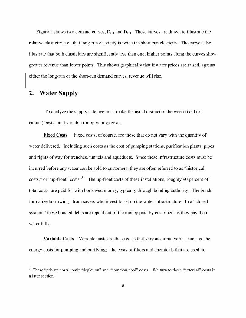
Figure 1 shows two demand curves, DSR and DLR. These curves are drawn to illustrate the
relative elasticity, i.e., that long-run elasticity is twice the short-run elasticity. The curves also
illustrate that both elasticities are significantly less than one; higher points along the curves show
greater revenue than lower points. This shows graphically that if water prices are raised, against
either the long-run or the short-run demand curves, revenue will rise.
2. Water Supply
To analyze the supply side, we must make the usual distinction between fixed (or
capital) costs, and variable (or operating) costs.
Fixed Costs Fixed costs, of course, are those that do not vary with the quantity of
water delivered, including such costs as the cost of pumping stations, purification plants, pipes
and rights of way for trenches, tunnels and aqueducts. Since these infrastructure costs must be
incurred before any water can be sold to customers, they are often referred to as “historical
costs,” or “up-front” costs. 3 The up-front costs of these installations, roughly 90 percent of
total costs, are paid for with borrowed money, typically through bonding authority. The bonds
formalize borrowing from savers who invest to set up the water infrastructure. In a “closed
system,” these bonded debts are repaid out of the money paid by customers as they pay their
water bills.
Variable Costs Variable costs are those costs that vary as output varies, such as the
energy costs for pumping and purifying; the costs of filters and chemicals that are used to
3 These “private costs” omit “depletion” and “common pool” costs. We turn to these “external” costs in a later section.

9
purify the water; repair and maintenance of the pipes and pumps used to distribute the water;
and the associated staffing. Unlike fixed “historical” costs, variable costs are inherently
contemporaneous.
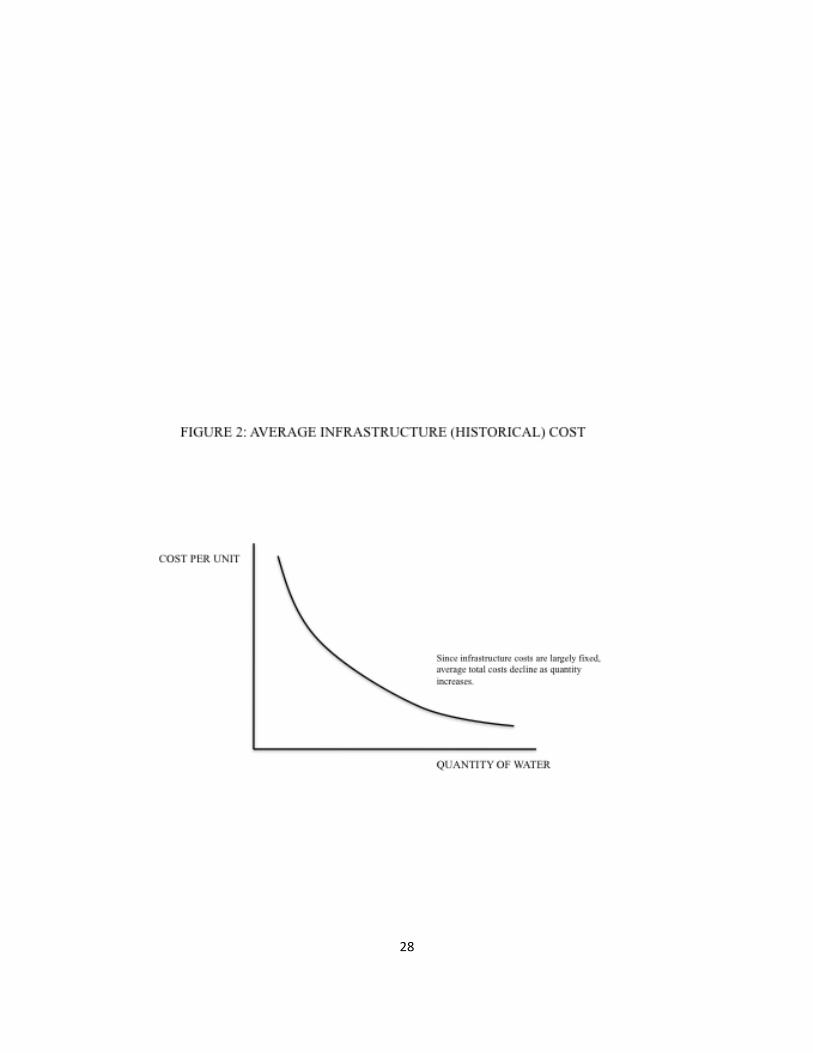
Average Cost Figure 2 shows the general shape of average costs of water delivery.
The horizontal axis shows the quantity of water delivered (Q) while the vertical axis shows the
price, measured in dollars per unit of water ($/Q). Because fixed costs dominate the total costs
of the typical water supply system, average cost curves are downward-sloping. Consequently,
water is usually supplied to urban areas by public water utilities operating as natural monopolies.
These utilities are regulated to prevent them from exploiting their single-seller advantage by
charging excessive monopoly prices. Such price regulation sets price maximums to limit the
return on investment to a “fair rate of return.”
3. Price Determination
Figure 3 is Fig. 2 plus the demand curve for water, D. To represent the empirical fact
that demand is highly inelastic, D is drawn with a steep slope. Because of relative inelasticity,
higher points on the demand curve represent higher revenue. The intersection of AC and D at
point A determines the price PAC that will just “recover” costs. That is, if PAC is charged, the
consumers will want to buy QAC, and the price per unit will equal the cost per unit, enabling the
utility to break even. 4
4 This price enables the water utility to cover all costs, including a fair rate of return on investments. That is, the opportunity cost of invested capital is included as a component of the average cost curve. Therefore, if price equals average cost, the revenue generated covers all costs.

10
Impact of Urban Out-migration on Price and Cost
As a significant segment of the urban population migrates toward newer cities and the
suburbs of older cities, those older cities are left with unused capacity in their water utilities.
The costs of the capacity must be paid for by those remaining urban resident rate-payers.
Figure 4 shows the effect of a population decline: the demand curve for water shifts from its
original position D1 leftward to D2. Consequently, the intersection with AC moves from point
A1 to point A2. Because the AC curve is downward-sloping, point A2 lies higher than point A1.
The price that will recover costs rises from P1 to P2 while quantity falls from Q1 to Q2. To
recover historical costs, the city must react to the out-migration by charging more per gallon to
sell water to the people who remain.5
Selling Water to Suburbs
The combination of highly inelastic demand and excess capacity gives the water works in
older Great Lakes cities a comparative advantage in reliable water supply. These cities can be
thought of as having two markets to serve: users in the city and users in the newer suburbs.
How much should be sold to each market and at what price? By selling water to the newer
surrounding suburbs, the city may be able to replace some of the tax revenue lost due to out-
migration. In turn, the suburbs may prefer to buy water rather than build their own water
utilities.
5 Usually the tax base per person also falls due to the out-migration: those who remain are usually of lower income than those who have left, and are less able to pay taxes.

11
We can use Figure 5 to show two alternative ways to sell water to suburbs using two
demand curves: DCITY shows the demand of the city residents and DCITY+SUBURB shows the
summation of the demands of the city residents and the suburban residents.6 In the first
alternative the utility can cover costs by charging city residents P2. Since revenue from city
users covers cost in this example, any additional revenue from sales to suburbs minus additional
costs of stretching the service out to those locations, is profit to the utility. For example, if the
city sells Q3 – Q2 to the suburb at price P3, and Q2 to city customers at price P2, then the profit
from suburban sales is shown by the rectangle HIJK. 7
The second alternative shown in Figure 5 is to recover cost while charging the same, or
“common” price to both the suburbs and the city. The common price P1 that will just recover
costs is determined at the intersection of DCITY+SUBURB and AC. Under this price structure, the
city water utility covers cost, including a fair rate of return to investors, but makes no profit.
Compared to the first alternative, this common price is lower to the city customers and much
lower to the suburban customers. In this case, the sales to the suburbs will be Q1 – Q4 while
sales to the city customers is Q4.
Selling water to suburbs gets more complicated when a second city attempts to sell water
to a suburb in rivalry with the first city. That is, suppose that city A wants to sell water to suburb
B but to complicate matters City C wants to start selling water to suburb B in rivalry with A.
City A can gain a “first-mover advantage” if it can be the first to reduce price, increase sales and
6 The demand curve of the suburbs need not be explicitly shown since, by construction, it is the horizontal gap between DCITY and DCITY+SUBURB
7 The PSC might object when the city earns revenue beyond cost recovery. As we will see, efficient prices are inherently above cost recovery.

12
thereby reduce average costs along its declining average cost curve. By moving first, A can
preempt sales by B, and the suburb enjoys the lower price. Moreover, because demand is
inelastic, the lower price results in less revenue to city A, lower water prices charged in the
suburbs and, consequently, a greater inducement to city residents to emigrate. From the city’s
point of view, this sequence contributes to a “race to the bottom.”
4. Water Depletion and Degradation Due to Commons Problems
It is well-known that both market systems and regulated utilities tend to under-price and
over-produce goods whose production generates an ignored external cost. In water economics,
external costs are present in two primary ways. First are the “common pool costs” that water
utilities impose on each other when they draw from a common source of water. The second
category of external costs consists of the inter-temporal depletion and degradation costs that
users of water today impose on future water users.
Common Pool External Costs
When cities draw water from the same aquifer, surface stream or lake, they impose costs
on each other. Each recognizes that their incentive to conserve the quality and quantity of water
is reduced by the ability of others to take what they attempt to save. Unless this perversity is
regulated, the common source of water is used at a rate far above the efficient rate.
Accelerated usage and/or degradation of the water is individually rational but collectively
irrational.8 But that is precisely what antiquated price regulation encourages.
8 The same “tragedy of the commons” principle applies to degradation of water quality as it does to depletion of its quantity.

13
The Costs of Aquifer Depletion
When water consumption today reduces the amount available to future users, water is
said to be depletable. Aquifer depletion occurs when water is drawn at a rate greater than the
natural “recharge.” 9 Costs rise with depletion since suppliers must bring water from greater
depths, and so drilling and pumping costs are greater. Moreover, at greater depths there is
increased risk of the infiltration of contaminants such as arsenic and radium, and, if public health
protection is to keep pace with the use of such water, adding costs of contaminant removal
before the water can be used. While these depletion costs are imposed on future users, they are
caused by usage today; they are a real cost of usage today. These “inter-temporal” costs of
action taken today are the subject of a vast literature on the economics of depletable resources.
Much of this literature is expressed in complex models.10 Fortunately, although the derivation
of the essential findings of inter-temporal resource economics cannot be shown with graphs, key
results can be built easily into the shape and interpretation of the marginal cost curve.11 In
inter-temporal economics the marginal cost of current usage of water includes not only the
familiar marginal production costs incurred today but also “marginal use” costs imposed on
future users due to the depletion and degradation associated with today’s water use.
9 Recharge is the replacement of water through rainfall or snow-melt. With respect to aquifers, depletion is often referred to as a drop in the water level, or “water table.”
10 A recommended primer on such models is Dorfman (1969). The inter-temporal economics of depletable resources is presented in papers by Loury (1978), Brown (1974), and the excellent book by Neher (1990). These advanced techniques are not a prerequisite to reading this section.
11 Depletion costs are prospective costs and are not included in accounting costs; unlike accountants, economists include depletion costs as part of marginal costs. Students of economics will recognize this as the distinction between implicit costs and explicit costs.

14
The marginal cost can be simply stated as a formula in three parts:
MARGINAL COST (MC) =
MARGINAL COST OF SUPPLY TODAY
+ MARGINAL COST IMPOSED TODAY ON OTHER SUPPLIERS IN THE
COMMON POOL
+ MARGINAL COST IMPOSED ON FUTURE SUPPLIERS DUE TO DEPLETION
AND DEGRADATION TODAY.
The first term is the conventional marginal production cost concept. To this well-known
textbook concept the next two less-familiar terms are added. The second term in the formula
above is the contemporaneous common-pool externality cost. The third term is the inter-
temporal depletion costs or “marginal-use costs,” i.e., the increased future cost incurred because
the resource is actually being depleted and perhaps degraded as it is being used. This equation
can therefore be read: the MC of water use today equals the marginal costs incurred today to
supply the water plus the marginal cost to other users of the common source plus the cost future
users will incur due to depletion or degradation of water resulting from use of water today.
Figure 6 shows all of the costs summed as an “all-inclusive” marginal cost curve.
Hereinafter we will refer to this simply as the MC curve, recognizing that environmental and
inter-temporal marginal costs must be included when referring to marginal cost. The curve is
upward-sloping beyond a minimum point, showing that common pool costs and depletion costs
contribute increasingly to marginal costs.

15
The stark difference between the downward-sloping retrospective AC curve and the
upward-sloping prospective MC curve shows the fundamental economics: an increase in the rate
of depletion of a water source causes the average cost to fall while it causes the marginal costs to
rise. Standard accounting reports will show falling retrospective average costs at higher sales
while society will suffer mounting prospective marginal costs. Put another way, accounting
costs and economic costs diverge in ways that accountants have no obligation to report and
hence decision-makers have no private incentive to acknowledge.12 In fact, common pool
problems are driven by opportunists who have a stake in perpetuation of inefficient regulation.
Paying a Royalty to the Future
Figure 7 adds the demand curve to Figure 6. As in Figure 3, the cost recovery price PAC
is determined at the intersection of demand and AC at point A. By contrast, the efficient price
is shown at point B where demand intersects MC: PMC = MC. Because MC lies above AC, the
intersection of MC with the downward-sloping demand curve at point B lies higher than the
intersection of demand and average cost at point A. Consequently, PMC must be greater than
PAC and QMC must be less than QAC.
In contrast to average-cost pricing which yields no profit, setting price equal to marginal-
cost does yield a profit since price is above average cost. Profit per unit is equal to PMC –
AC(QMC), shown by the distance BC. This price gap above average cost is the royalty rate per
unit paid to the future. Total profit is BC times quantity, shown by the rectangular area BCFG.
12Failure to recognize these costs when making decisions is the essence of the externality problem.
16
To capture inter-temporal efficiency, people in the future must actually receive the
benefit of this royalty. To bequeath this benefit, this profit should be spent on investment to
provide capital-based economic growth that the future citizens can eventually enjoy. That is, the
“royalty paid to the future” cannot be spent on consumption today. Instead, the only way the
future citizens can receive this benefit is for the increased price paid today to be invested in
economic growth through capital investment. This policy could be implemented by reduction of
tax rates or financial support for some other social capital investment such as education or debt
reduction.13
Although average cost pricing is a guarantor of cost recovery and is the most common
form of regulated water pricing, economists prefer the efficiency of marginal cost pricing.
Economic efficiency requires that price equals marginal cost: price acts as a signal to users
that they should adjust their usage so that the rate at which benefits are derived from usage (P)
equals the rate at which the system bears costs to serve them (MC). 14
An additional advantage of marginal over average cost price regulation lies in how the
two policies deal with changing demand. We have seen earlier that with average cost price
13 This is a corollary to the general “Pigouvian” remedy for imperfections in the market: increase taxes to discourage production of those things we want less of, and decrease taxes on or increase subsidies of the production of those things we want more of. See Arthur Pigou (1912).
14 When economists advocate marginal cost pricing for water they usually arouse the ire of consumer advocates and business advocates alike. Efficient prices are higher than the cost-recovery prices people have gotten used to, often much higher. More important, these prices are calculated in a different way than people are used to – i.e., prospectively rather than retrospectively. Interested parties often rebel at having to pay prices higher than they are familiar with paying, especially for a very necessary service like water. Economists often refer to this extra payment as “a royalty paid to the future.” Because this royalty is not required to sustain current operations there will be pressure to cut price and be a free rider on the future instead of paying the royalty.

17
regulation an increase (decrease) in demand will cause price to fall (rise). That is, because the
AC curve is downward-sloping, the less the demand, the higher the price the demanders must
pay to cover historical costs. This increase in price in response to reduced demand creates
perverse incentives: conservation is punished by higher prices, and increased sales of the
depletable resource are rewarded by a lower price.
Just the opposite is true with marginal-cost pricing. To see this, suppose demand declines
while the water utility is charging P = MC. As the demand curve shifts left against the upward-
sloping marginal cost curve, the intersection occurs at a lower price. Conservation is rewarded
by a lower price and the royalty owed to the future by current users is reduced because current
usage is less. Less compensation is required since less cost is imposed on the future. In
summary, marginal cost water pricing sets the right price at each point in time; price creates the
efficient incentives for current users to use water taking into account costs imposed on future
users of water. In contrast to average cost pricing, users subject to marginal-cost pricing need
not fear that collective conservation will perversely result in higher water rates. Users have an
ongoing incentive to invest in water-saving devices, and the price generates a capital fund.
Improvements in the current debt structure of cities are one obvious way to use such a capital
fund, handing the future less debt.
There is a danger in collecting all this revenue in excess of what is required for current-
period operating cost and bond redemption: the money could be captured by opportunists in the
name of beneficent “economic growth.” This is always a danger when efficiency prices are
charged, and the public must be on guard. Economics teaches us to spend the money on broad

18
range investments that improves the competitive process, not attempting to “pick winners”
among individual competitors.
5. Non-Linear Price Policy: Block Pricing
Discussions of water pricing are incomplete without consideration of poor people.
Fortunately, the arsenal of economics includes many ways to help the poor while employing
efficient price incentives. The easiest method is simply to provide a rebate when people pay
their income taxes. Rebates for higher water bills would simply add to the familiar rebate
programs that assist with heating and rental payments.
If using the tax code is not a popular idea, then another tool in the economists’ tool kit
can be used: non-linear pricing. Price need not be the same for all units of water sold; “block
pricing” can be used to encourage either more water usage or less water usage, depending on
whether price rises or falls with successive blocks of usage. Fig. 8(a) shows an increasing-block
price structure. The price equals Po per gallon for the first “block” of 30 gallons per day, rising
to P1 per gallon for additional use beyond that first block. Such a price schedule enables users
to pay less for the first block and pay the higher price only if their consumption exceeds that first
trigger-quantity of water. The desire to avoid the higher price block encourages water
conservation and, in turn, the purchase of water-conserving appliances and equipment. Sellers of
such products would benefit from an increase in demand.

19
Panel (b) shows decreasing block pricing (DBP). DBP schedules are popular with large
industrial users of water like breweries and paper companies.15 Under this DBP schedule the
price falls after a large quantity block is used; in this example the trigger quantity is 30,000
gallons per day. Compared to increasing block pricing, decreasing block pricing yields less
profit for the water utility and encourages greater water use, violating the rules of economic
efficiency since the marginal price the user pays falls below the long-run marginal cost.
Cities and regions anxious to please large employers often charge DBP as an enticement
to create jobs or to retain existing jobs. Note that this job-creation motive is at odds with the
inter-temporally efficient rate of water use. Competition among regions to attract employers
through under-priced water -- increasing water use in order to create jobs -- is a form of the
common pool problem. Each region, especially those with serious employment problems, will
be tempted to play this role in the tragedy of the commons.
Price Elasticity and IBP
IBP separates the essential uses of water from the more optional uses and subjects these
different demands to different prices. In Fig. 9(a) the demand curve for essential uses reflects
both low elasticity and low quantity. Panel (b) shows the demand curve for relatively optional
but high-volume uses, such as landscaping, swimming pools and hot tubs. Note that the demand
curve in panel (b) shows much greater quantity demanded at any price as well as greater price
elasticity. By keeping the price low for the low-volume essential uses, while imposing the
15 One proffered justification for DBP is that high-volume, or “wet industries”, pay their fair share of infrastructure costs by their payment for the first block, and that further blocks should therefore be sold to them at a lower price.

20
higher price on the higher volume, relatively optional uses of water, IBP separates these
demands.
In Fig. 9, the price charged for the first 50 gallons per day is Po, and, at that price, the
demander shown in panel (a) chooses 25 gallons per day for essential uses. Panel (b) shows how
this same demander reacts to IBP when choosing how much water to buy for optional uses. Note
that the price line in panel (b) is affected by the decision made in panel (a). Since Po applies to
the first 50 gallons but this consumer uses only 25 gallons for essential uses: she is entitled to
25 more gallons at that price. Therefore, the first 25 gallons of optional water use in panel (b)
are also sold at Po.16 At point B’, however, the fifty-gallon trigger quantity is reached and the
higher price kicks in, raising the price to P1, and inducing the consumer to choose 100 gallons
per day of optional uses plus the 25 gallons for essential uses. If the price had been Po for all
water used, both essential and optional, the consumer would have chosen a quantity demanded of
200 gallons of water for optional uses. With IBP, the consumer facing P1 cuts optional usage by
50% from 200 to 100.
Economists point out four advantages when they prescribe IBP pricing to regulate water
use. First, while water is essential for life, not all uses of water are essential. Second, essential
uses tend to be low-volume while more optional uses are typically high-volume uses. Third,
although demand is very inelastic for essential uses of water, demand is more elastic for more
optional uses. The non-linear IBP price line provides a separation of these demands. Fourth,
16 To derive panel (b), draw the demand curve for the essential uses of water in panel (a) first; establish the quantity demanded at the price-break; and then proceed to draw the price hike for the remaining quantity of water demanded. For an extensive discussion of increasing-block pricing, see Olmstead, et al (2009).

21
because IBP is a price system and not a command and control regulation, IBP leaves the rate of
usage up to the user instead of direct government intrusion into personal decision-making.
Many oppose price regulation in fear of losing a familiar right to use water as they wish,
regardless of economic efficiency. In a world of increasing scarcity, however, that “right” is
increasingly unsustainable. To achieve sustainability, economics offers proper pricing as the
way to preserve the right to use water efficiently. The efficient usage of a depletable resource
like water can preserve much of the current way of life and forestall or avoid the need to invoke
heavy handed command and control practices as water supplies diminish.
6. Conclusion
Microeconomics suggests two ways to look at the demand-side for water. The first is
elasticity, both short and long-run. The consensus estimate of long run elasticity of demand is .6
while for the short run the consensus is .3. Both figures are significantly less than 1.0, which
means that while a price increase decreases the quantity demanded, it also increases sales
revenue.
The second way to look at the demand for water is to distinguish between essential uses
of water – e.g., cooking and health-related uses -- versus more optional uses – e.g., landscaping
and recreational uses. The economists’ tool-kit includes non-linear pricing which can be
designed to permit users to pay lower prices for a small quantity of water per day, but higher
22
prices for additional quantities. Such increasing-block pricing induces conservation while
keeping prices lower for the essential uses of water.
The supply side is complicated by both the structure of high infrastructure costs and the
“tragedy of the commons” which leads to resource depletion and degradation. Due to high fixed
infrastructure costs, most water utilities are natural monopolies and are typically price-regulated
to recover infrastructure costs. However, efficiency requires that price cover not only marginal
supply cost but also the common-pool externality costs plus the “marginal use cost” imposed
on future users due to depletion and degradation of water today. That is, to induce efficiency
users must “pay a royalty to the future.”
Great Lakes cities typically have excess water infrastructure capacity, earned the hard
way through heavy investment followed by loss of population and economic activity. This
excess capacity in reliable water supply gives these cities what David Ricardo would dub a
“comparative advantage” in reliable water supply. Ricardo (1817) recognized that any
economic entity – country, region, firm, household – should maximize the value of what it does
better than others, and then trade for what others do better. The analogy for the Great Lakes
Cities is to maximize the value of reliable water supply and trade for a wide and stable array of
economic activity. The challenge for policy makers in these older cities is to maximize the
economic value of this comparative advantage while at the same time sustain the environment.
Through proper pricing, the comparative advantage can be maximized through sales to city
residents, suburban customers, and new residential and business users of water attracted by
efficient use of the revenue generated by efficient pricing.

23
Fortunately, since the demand for water is very inelastic, higher prices serve both the goal
of raising revenue and the goal of preserving the environment. The older cities badly need
revenue to enhance economic development, which depends upon quality of life, schools, public
health, and a host of other characteristics including tax rates. Meanwhile, climate change is
making reliable water supply increasingly valuable as competing supplies elsewhere “dry up.”
Just as any business firm would raise price in response to increased competitive advantage, Great
Lakes states can raise water prices as their reliable supplies become increasingly in demand. In
addition, higher water prices will encourage conservation of water, support water-conserving
land-use patterns, and stimulate demand for water saving appliances and equipment - products
that local firms are keen to sell.
Some Great Lakes cities, including Erie, PA, and Milwaukee, Wisconsin have proposed
to offer low-priced or free water to entice water-intensive, job-creating firms to relocate to their
cities, using water as a kind of “commodity currency” to subsidize water-intensive firms. In
Milwaukee, the popular proposal is to create WAVE districts, where the acronym stands for
“Water Attracts Valued Employers.” WAVE districts are essentially barter arrangements in
which water is exchanged for job creation in, say, a new bottling plant.
Economics warns of three problems with barter. First, in general money is a better
medium of exchange than bartered commodities: the revenue derived from water sales can
serve as a better inducement for firms to relocate to the older cities than can the water itself.
The revenue derived from water sales can be used to improve the business climate for a broad
array of job-creating activity -- letting the market decide the mix of commercial and residential
activity that is best for the city -- than can the narrower enticement of water itself.

24
Second, the lower prices inherent in the barter arrangement will slow the investment in
water-conserving equipment and infrastructure.
Third, David Ricardo’s bedrock principle of comparative advantage teaches us to
maximize the value of our comparative advantage and then trade for a broad array of “imports”
that others have comparative advantage in producing. Implementing this lesson, older cities
should maximize the value of the reliable water supply by raising the price, and using the
revenue to “import” a broad array of firms to relocate to create jobs -- whether those firms are
wet, dry or damp -- as well as residential development. This revenue can be used to reverse the
vicious cycle of higher tax rates and emigration to the suburbs. Instead, the revenue can be used
to create a virtuous cycle, revitalizing the city and reducing city tax rates in an effort to expand
the tax base, and entice residential and commercial activity to relocate within the city. This
would be an especially good time to attract baby-boomer empty nesters to the city, thereby,
increasing the tax-base per acre while also contributing to the economic and cultural life.

25
REFERENCES
Baumann, D. D., Boland, J.J., and Hannemann, W. M. 1998 Urban Water Demand Management and Planning. McGraw-Hill, Inc. (New York)
Brown, G.M. 2000 Renewable Natural Resource Management and Use Without Markets. Journal of Economic Literature, Vol. 38, No. 4 875 – 914
Brown, G.M. 1974 An Optimal Program for Managing Common Property Resources with Congestion Externalities. The Journal of Political Economy, Vol. 82, No. 1 pp. 163-173
Dorfman, R.. 1969. An Economic Interpretation of Optimal Control Theory. American Economic Review, Vol. 59, No. 5 (Dec, 1969), pp. 817-831
Gleick, P.H., et al. 2008 – 09 The World’s Water, The Biennial Report on Freshwater Resources. Island Press (Washington, D.C.)
Hanemann, W. M. , Olmstead, S.M., and Stavins, R. N. 2007. Water Demand Under Alternative Price Structures. Journal of Environmental Economics and Management 54(2), 181 - 198
Hirshleifer, J., DeHaven, J.C., and Millman, J.W. 1960 Water Supply, Economics, Technology, and Politics. The Rand Corporation (Santa Monica)
Loury, G.C. 1978 The Optimal Exploitation of an Unknown Reserve. The Review of Economic Studies, Vol. 45, No. 3, pp. 621-636
Mansur, E. T. and Olmstead, S. M. 2005. The Value of Scarce Water: Measuring the Inefficiency of Municipal Regulations,
Neher, P. A. 1990 Natural Resource Economics: Conservation and Exploitation (Cambridge University Press)
Olmstead, S. M. 2009. Reduced-form vs. Structural Models of Water Demand Under Nonlinear Prices. Journal of Business and Economic Statistics 87(1), 84 – 94.
Olmstead, S. M. and Stavins, R. N. 2009. Comparing Price and Non-price Approaches to Urban Water Conservation. Water Resources Research, forthcoming
Olmstead, S. M., Hanemann, W.M., and Stavins, R. N. 2007 Water Demand Under Alternative Price Structures. Journal of Environmental Economics and Management 54(2), 181-198
Pigou, A. C. , 1912 Wealth and Welfare Oxford University Press (Oxford, UK)

26
Ricardo, David. 1817 On the Principles of Political Economy and Taxation, Cosimo Classics (1990).

27
28

29

30

31

32

33

34

35