Embed Size (px)
Citation preview

Microeconomics II: Trade
Program in Economic Policy Management U4613
Lecture Notes
Kenneth L. Leonard
Spring, 2001

Contents
1 The Ricardian Model 7
1.1 Introduction . . . . . . . . . . . . . . . . . . . . . . . . . . . . . . . . 7
1.1.1 Quiz . . . . . . . . . . . . . . . . . . . . . . . . . . . . . . . . 7
1.1.1.1 What do we learn from this exercise? . . . . . . . . . 9
1.2 One country, two goods, one factor . . . . . . . . . . . . . . . . . . . 10
1.2.1 Determination of Prices . . . . . . . . . . . . . . . . . . . . . 12
1.2.1.1 Note on the shape of the PPF . . . . . . . . . . . . . 13
1.2.2 Small country facing world prices . . . . . . . . . . . . . . . . 14
1.3 Two countries, two goods, one factor . . . . . . . . . . . . . . . . . . 14
1.3.1 Flat production possibility frontier . . . . . . . . . . . . . . . 17
1.3.2 Wages . . . . . . . . . . . . . . . . . . . . . . . . . . . . . . . 19
1.3.3 False Views of Trade . . . . . . . . . . . . . . . . . . . . . . . 19
2 Specific Factors Model 20
2.1 Introduction . . . . . . . . . . . . . . . . . . . . . . . . . . . . . . . . 20
2.2 Graphical Representation . . . . . . . . . . . . . . . . . . . . . . . . . 20
2.3 Changes in the Price Ratio . . . . . . . . . . . . . . . . . . . . . . . . 24
2.3.1 Equi-proportional changes in prices . . . . . . . . . . . . . . . 24
2.3.2 Differential changes in prices . . . . . . . . . . . . . . . . . . . 24
2.3.2.1 Earnings of Capital . . . . . . . . . . . . . . . . . . . 25
2.3.2.1.1 Earnings of Landowners . . . . . . . . . . . 26
2.3.2.1.2 Earnings of Labor . . . . . . . . . . . . . . 27
2.3.3 Graphical Representation of Changes in Wages . . . . . . . . . 28
2.4 Implication of the Model . . . . . . . . . . . . . . . . . . . . . . . . . 29
2.5 Political Economy Considerations . . . . . . . . . . . . . . . . . . . . 30
1
3 Factor Proportions Model (Heckscher–Ohlin Model) 31
3.1 Introduction . . . . . . . . . . . . . . . . . . . . . . . . . . . . . . . . 31
3.2 Fixed Coefficients Model . . . . . . . . . . . . . . . . . . . . . . . . . 31
3.2.1 Impact of Prices . . . . . . . . . . . . . . . . . . . . . . . . . . 34
3.2.2 Prices and Factor Incomes . . . . . . . . . . . . . . . . . . . . 35
3.3 Numerical Example, Magnification Effect in the Stolper–Samuelson
Theorem . . . . . . . . . . . . . . . . . . . . . . . . . . . . . . . . . . 37
3.4 Variable Coefficients . . . . . . . . . . . . . . . . . . . . . . . . . . . 39
3.4.1 Lerner Diagram . . . . . . . . . . . . . . . . . . . . . . . . . . 41
3.4.1.1 Fix factor prices, derive goods prices . . . . . . . . . 41
3.4.1.1.1 Fix goods prices, derive factor prices . . . . 41
3.4.2 Impact of Changing Prices . . . . . . . . . . . . . . . . . . . . 41
3.4.3 More on the Relationship between goods prices and factor prices 44
3.5 Stolper–Samuelson . . . . . . . . . . . . . . . . . . . . . . . . . . . . 45
3.6 Capital-Labor Ratio and Specialization . . . . . . . . . . . . . . . . . 45
3.7 Allocation of Resources to Production . . . . . . . . . . . . . . . . . 46
3.8 Biased Expansion of the PPF . . . . . . . . . . . . . . . . . . . . . . 47
3.9 Conclusions . . . . . . . . . . . . . . . . . . . . . . . . . . . . . . . . 53
4 Basic Trade Policy and Welfare Analysis 54
4.1 Introduction . . . . . . . . . . . . . . . . . . . . . . . . . . . . . . . . 54
4.2 Rent seeking activities with quotas and import licenses . . . . . . . . 54
5 Import Substituting Industrialization 56
5.1 Introduction . . . . . . . . . . . . . . . . . . . . . . . . . . . . . . . . 56
5.2 The policy of Import Substituting Industrialization and Infant Industry
Protection . . . . . . . . . . . . . . . . . . . . . . . . . . . . . . . . . 58
5.3 An example of ISI with declining costs . . . . . . . . . . . . . . . . . 58
5.3.1 Government Intervention . . . . . . . . . . . . . . . . . . . . . 59
5.3.2 Private Market reactions to Declining Costs . . . . . . . . . . 60
5.4 Externalities . . . . . . . . . . . . . . . . . . . . . . . . . . . . . . . . 60
5.4.1 Appropriable Technology . . . . . . . . . . . . . . . . . . . . . 62
5.4.1.1 Example of Spillovers from Investment in Technology 62
5.4.2 On-the-job training . . . . . . . . . . . . . . . . . . . . . . . . 64
5.4.3 Static Externalities . . . . . . . . . . . . . . . . . . . . . . . . 66
5.4.4 Imperfect Information . . . . . . . . . . . . . . . . . . . . . . 66
2

5.5 Backward Linkages . . . . . . . . . . . . . . . . . . . . . . . . . . . . 66
5.6 Latin American Experience . . . . . . . . . . . . . . . . . . . . . . . 66
6 Monopolistic Competition and World Trade Patterns 67
6.1 Introduction . . . . . . . . . . . . . . . . . . . . . . . . . . . . . . . . 67
6.2 Monopolistic Competition . . . . . . . . . . . . . . . . . . . . . . . . 68
6.2.1 Costs and number of firms . . . . . . . . . . . . . . . . . . . . 70
6.2.2 Firm level profit maximization and number of firms . . . . . . 70
6.2.3 Equilibrium . . . . . . . . . . . . . . . . . . . . . . . . . . . . 71
6.2.4 Numerical Example of Monopolistic Competition . . . . . . . 71
References 73
Index 76
Glossary 76
3

List of Figures
1.1 PPF of Bread and Wine for weak . . . . . . . . . . . . . . . . . . . 10
1.2 PPF with two hypothetical relative prices . . . . . . . . . . . . . . . 11
1.3 Typical PPF, utility, price graph . . . . . . . . . . . . . . . . . . . . 12
1.4 PPF with one specialized unit of Labor . . . . . . . . . . . . . . . . . 14
1.5 Advantages of Trade at given prices . . . . . . . . . . . . . . . . . . . 15
1.6 Derivation of the Export Supply Curve: I . . . . . . . . . . . . . . . . 16
1.7 Derivation of the Export Supply Curve: II . . . . . . . . . . . . . . . 16
1.8 PPF of weak and strong . . . . . . . . . . . . . . . . . . . . . . . 17
1.9 World Supply of Bread . . . . . . . . . . . . . . . . . . . . . . . . . . 18
2.1 PPF with Specific Factors: Labor Allocation . . . . . . . . . . . . . . 21
2.2 PPF with Specific Factors: Deriving the PPF . . . . . . . . . . . . . 22
2.3 PPF with Specific Factors: Distribution of Labor . . . . . . . . . . . 23
2.4 Finding the APLM and MPLM with diminishing returns to labor . . 26
2.5 APLM and MPLM with diminishing returns to labor . . . . . . . . . 27
2.6 Graphical Representation of Equilibrium in Wages . . . . . . . . . . . 28
2.7 Graphical Representation of Change in Relative prices . . . . . . . . 28
2.8 Graphical Representation of Capitalist Income . . . . . . . . . . . . . 29
3.1 Deriving the PPF with Fixed Coefficients . . . . . . . . . . . . . . . . 32
3.2 Fixed Coefficients PPF, increasing Labor Supply . . . . . . . . . . . . 33
3.3 Impact of various price ratios on production decision . . . . . . . . . 34
3.4 Equilibrium in the wage and rental market for factors . . . . . . . . . 35
3.5 Prices of Cloth and Food and the Wage and Rent Equilibrium . . . . 36
3.6 Isoquants . . . . . . . . . . . . . . . . . . . . . . . . . . . . . . . . . 40
3.7 Isoquants and Constant Returns to Scale . . . . . . . . . . . . . . . . 41
3.8 The unit isoquant and isocost frontiers . . . . . . . . . . . . . . . . . 42
3.9 Wage, rent ratios and the capital-labor ratio . . . . . . . . . . . . . . 42
4

3.10 Relationship between wr
and k . . . . . . . . . . . . . . . . . . . . . . 43
3.11 The Lerner Diagram . . . . . . . . . . . . . . . . . . . . . . . . . . . 43
3.12 Deriving relationship between goods price ratios and factor price ratios 44
3.13 The relationship between goods price ratios and factor price ratios . . 45
3.14 Prices, wage-rent ratios and capital labor ratios . . . . . . . . . . . . 46
3.15 Prices, wage-rent ratios and capital labor ratios . . . . . . . . . . . . 47
3.16 Allocation of resources in Heckscher–Ohlin economy . . . . . . . . . . 48
3.17 Increase in supply of capital . . . . . . . . . . . . . . . . . . . . . . . 49
3.18 Biased Expansion of the PPF: I . . . . . . . . . . . . . . . . . . . . . 50
3.19 Biased Expansion of the PPF: II . . . . . . . . . . . . . . . . . . . . . 50
3.20 Two countries begin identical: Add small amount of capital to A’s
resources: I . . . . . . . . . . . . . . . . . . . . . . . . . . . . . . . . 51
3.21 Two countries begin identical: Add small amount of capital to A’s
resources: II . . . . . . . . . . . . . . . . . . . . . . . . . . . . . . . . 51
5.1 Real Non-Oil Commodity Terms of Trade, 1977-1992 . . . . . . . . . 57
5.2 Declining terms of trade leads to declining welfare . . . . . . . . . . . 57
5.3 Pre-Intervention production and consumption for import competing
good . . . . . . . . . . . . . . . . . . . . . . . . . . . . . . . . . . . . 59
5.4 Production and consumption for import competing good with Tariff . 60
5.5 Production and consumption for import competing good with Forward–
Looking company . . . . . . . . . . . . . . . . . . . . . . . . . . . . . 61
5.6 Private PPF for farmer engaged in research . . . . . . . . . . . . . . 63
5.7 Social and Private PPF for farmer engaged in research . . . . . . . . 64
5.8 Free Riding with spillovers . . . . . . . . . . . . . . . . . . . . . . . . 65
6.1 Profits driven to zero in Monopolistic Competition . . . . . . . . . . 69
5
List of Lectures
January 16th, 2001 . . . . . . . . . . . . . . . . . . . . . . . . . . . . . . . . . . . . . . . . . . . . . . . . . . . . . 7—11
January 18th, 2001 . . . . . . . . . . . . . . . . . . . . . . . . . . . . . . . . . . . . . . . . . . . . . . . . . . . . 11—18
January 23rd, 2001 . . . . . . . . . . . . . . . . . . . . . . . . . . . . . . . . . . . . . . . . . . . . . . . . . . . . 19—19
January 23rd, 2001 2nd lecture . . . . . . . . . . . . . . . . . . . . . . . . . . . . . . . . . . . . . . . . 20—26
January 30th, 2001 . . . . . . . . . . . . . . . . . . . . . . . . . . . . . . . . . . . . . . . . . . . . . . . . . . . . 24—30
February 1st, 2001 . . . . . . . . . . . . . . . . . . . . . . . . . . . . . . . . . . . . . . . . . . . . . . . . . . . . . 31—36
February 5th, 2001 . . . . . . . . . . . . . . . . . . . . . . . . . . . . . . . . . . . . . . . . . . . . . . . . . . . . 36—41
February 8th, 2001 . . . . . . . . . . . . . . . . . . . . . . . . . . . . . . . . . . . . . . . . . . . . . . . . . . . . 41—46
February 20th, 2001 . . . . . . . . . . . . . . . . . . . . . . . . . . . . . . . . . . . . . . . . . . . . . . . . . . . 45—49
February 22nd, 2001 . . . . . . . . . . . . . . . . . . . . . . . . . . . . . . . . . . . . . . . . . . . . . . . . . . . 52—53
6

Chapter 1
The Ricardian Model
01/16/01⇓
1.1 Introduction
1.1.1 Quiz
There are two countries, strong and weak. They have the following endowmentsand production capacities:
Country strong weakTotal Labor Units 4 3number of each good that can beproduced with 1 unit of laborbread (slices) 4 3wine (glasses) 3 1
1. Which country has more resources?
• strong
2. Which country is more efficient at producing bread?
• strong
3. Which country is more efficient at producing wine?
• strong
4. Assume that units of labor cannot be split – you cannot use 1.5 units of labor,only 1 or 2, for example. List all possible outputs for strong and weak. Putyour answer in the table below where each row represents a possible combinationof units of bread and wine. [There is no trade.]
7

strongbread wine
labor output labor output4 16 0 03 12 1 32 8 2 61 4 3 90 0 4 12
weakbread wine
labor output labor output3 9 0 02 6 1 11 3 2 20 0 3 3
5. Assume that each country gets utility from consuming bread and wine andthat they prefer to consume them in combination than to consume them alone.Bread tastes better with wine, and wine tastes better with bread. Utility is theproduct of bread and wine. Thus 4 units of bread and 2 units of wine has autility of 8. [There is no trade.]
Show all possible utilities for strong and weak.
strongbread wine utility
16 0 012 3 368 6 484 9 360 12 0
weakbread wine utility
9 0 06 1 63 2 60 3 0
6. Now we will allow strong and weak to trade with each other. Assume thatstrong chooses to produce at the point where its utility was maximized whenthere was no trade. If weak chooses to produce only bread is there any offer oftrade that she can make to strong which will make both weak and strongbetter off (in terms of utility) than at any other possible production point? Ifso, what trade is this (assume that only whole units of any good can be traded)and what is the resulting utility for both strong and weak?
• strong starts at 8 slices of bread and 6 glasses of wine for a utility of 48.weak starts at 9 slices of bread and no glasses of wine. If weak offersstrong 2 slices of bread for 1 glass of wine, weak ends up with 7 and 1for a utility of 7, which is higher utility than for any other combination ofproduction without trade.
• Will strong accept? strong ends up with 10 slices of bread and 5glasses of wine, for a utility of 50. strong is better off than with anyother non-trade form of production. strong will accept.
7. Again assume that strong produces at the point where its utility was maxi-mized before trade. Now assume that weak produces only wine. Is there any
8

offer of trade that she can make to strong which will make both weak andstrong better off (in terms of utility) than at any other possible productionpoint? If so, what trade is this and what is the resulting utility for both strongand weak?
• weak produces no bread and 3 glasses of wine. weak could trade 1 glassfor 1 slice, 1 glass for 2 slices, 1 glass for 3 slices or 1 glass for 4 slices.What can these trades do?
trade totalbread wine bread wine utility
1 1 1 2 22 1 2 2 43 1 3 2 64 1 4 2 8
• Only the last of these trades makes weak better off. Would strongaccept this trade? If strong gives up 4 slices of bread for 1 glass of winestrong ends up with 4 and 7 for a utility of 28. strong would not acceptthis trade. Would strong accept the next best trade (which wouldn’tmake weak better off, but wouldn’t make weak worse off either)? Herestrong would end up with 5 and 7 for a utility of 35. strong would notaccept this either.
1.1.1.1 What do we learn from this exercise?
The titles strong and weak were deliberately chosen because they have meaning
in this exercise. weak has less resources and is less efficient.
• The existence of gains from trade does not depend on equality of resources or
the ability of a country to produce goods more efficiently than another. (If we
generalize from weak to a country that is not more efficient than any other
country at producing anything, we can still get gains from trade).
• Although trade is advantageous both nations, only a particular type of trade
is advantageous. In particular weak does not gain by trading wine for bread,
only by trading bread for wine.
• We will use the term absolute advantage to capture the fact that strong is
more efficient than weak at producing both wine and bread. [strong has an
absolute advantage in the production of both wine and bread.]
• We will use the term comparative advantage to capture the fact that weak
appears to be better off if it produces some bread to trade with strong for
9

wine. [weak has a comparative advantage in the production of bread.]
1.2 One country, two goods, one factor
We will now generalize from these results, and allow continuous allocation of labor.
There is one country, weak, with the following endowments and production capaci-
ties:Country weakTotal Labor Units 10number of each good that can beproduced with 1 unit of laborbread (slices) 3wine (glasses) 1
Definition 1 aLB is the number of units of labor required to make 1 slice of bread
[productivity of labor per unit of bread].
Definition 2 aLW is the number of units of labor required to make 1 glass of wine
[productivity of labor per unit of wine].
wine
breadL
aLB= 30
LaLW
= 10 ︷︸︸︷3 slices of bread
} 1 glass of wine
Figure 1.1: PPF of Bread and Wine for weak
Figure 1.1 tells us what can be physically produced in the weak economy; the
production possibility frontier In order to know what will actually be produced we
need to know something about prices, or actually relative prices. As you might
suspect, how much of each good is actually produced does not depend on the actual
prices, but the ratio of prices. If bread is three times as expensive as wine, that is
enough information to tell us what should be produced, we do not need to know the
actual price of bread.
10

In Figure 1.2 we draw the production possibility frontier and two hypothetical
price ratio. In fact, the price ratio only tells us the slope of the price line, it does
not tell us the intercept. The slope is the negative of the price of wine over the price
of bread. All the slopes that we discuss are in fact negative slopes (they point down
when viewed from left to right), but this is confusing notation. We will talk about
slopes as if they were positive (omitting the negative sign and if the slope is steeper we
will say the slope is larger.) This is the equivalent of talking only about the absolute
value of the slope.
We choose the intercept for each price line by making sure that the price line
touches at least part of the production possibility frontier. In this way we use the price
ratio to construct a budget constraint. Any point along or inside of the production
possibility frontier represents a possible output of the economy. The budget constraint
represents all the points that are possible with trade. If you can produce at any point
along a price line, with trade you can consume at any other point along the price line.
Thus, prices allow us to examine both the production possibility frontier and what I
will call the “trade–augmented production possibility frontier”.
PPPPPPPPPPPPPPPPPP
bread
wine Slope is aLB
aLW
?
PB
PW> aLB
aLW
PB
PW< aLB
aLW
?
?
Figure 1.2: PPF with two hypothetical relative prices
01/18/01⇓ 01/16/01⇑ If PB
PW> aLB
aLW, then the economy will specialize in the
production of bread. To see this look at the total earnings of the economy when
it produces only bread, we introduce a new variable, x which is the units of labor
11

devoted to the production of wine.
Revenue R =L− x
aLB
· PB +x
aLW
· PW
∂R∂x
=−PB
aLB
+PW
aLW
∂R∂x
< 0 ifPB
aLB
>PW
aLW
or ∂Rδx
< 0 ifPB
PW
>aLB
aLW
When the derivative of revenues with respect to x is negative, revenues are increased
by decreasing production of wine, in this case producing zero glasses of wine.
If PB
PW< aLB
aLW, then the economy will specialize in the production of wine. Follow
the same exercise as above to show this.
1.2.1 Determination of Prices
When we are looking at only one country (in this case weak), it doesn’t make much
sense to just declare a set of prices. They have to come from somewhere. Prices
in a closed economy reflect the preferences of the individuals in that economy for
the goods being produced. In order to determine the prices in a closed economy,
we usually need to know the demand as well as the supply. Demand in this case is
represented by a utility map. The usual representation of the determination of prices
is shown in Figure 1.3.
Good A
Good B
Utility
PPF
Ratio of Prices
Figure 1.3: Typical PPF, utility, price graph
The combination of the production possibility frontier and utility gives us a unique
12

set of relative prices for this closed economy. Note that if the production possibility
frontier is flat then all possible utility functions (non-trivial and convex) give the
same set of prices. The line1 that separates the production possibility frontier and
the highest obtainable iso-utility curve has exactly the same slope as the production
possibility frontier at the point of contact, and when the slope of the production
possibility frontier is the same over the whole set, then we automatically know the
ratio of prices.
1.2.1.1 Note on the shape of the PPF
Note that in Figure 1.3 the production possibility frontier is bowed outward or con-
cave.
Question 1 Why do we usually represent the production possibility frontier as con-
cave?
This is basically the result of diminishing returns to any given factor.
In the case of only one input, concavity may be the result of differentiation in
units of input. If there is one unit of the productive input that is more efficient at
producing one input than any of the other inputs (one unit of labor that is really good
at producing bread, or one plot of land that is very productive), then when we pass
this unit from wine to bread, we get a flatter slope than for the rest of the production
possibility frontier (see Figure 1.4).
In the case of multiple inputs, this intuition still holds. There are some units of
any given factor that are just better suited to producing certain types of goods. When
we shift these last factors over we get less.
Question 2 Why do we usually represent the iso-utility graph as convex?
Convexity in iso-utility curves is the result of preferences for bundles over extremes.
This is easy to visualize with the definition of a convex set.If we choose any two points
on the iso-utility graph we can see that any combination of these points (any point
along a line drawn between the points) give higher utility than either of the two points:
combinations are preferred over extremes).
13

cc
cc
cc
cc
cc
cc
Bread
Wine
Flat PPF (all factors identical)
Concave PPF (One unit of labor highly specialized)
Specialized Unit moving from Wine to Bread
?
�
?
Figure 1.4: PPF with one specialized unit of Labor
1.2.2 Small country facing world prices
Figure 1.5 shows the same small country as in Figure 1.3, except that in this case
there is a set of world prices, as well as the domestic prices. We assume that weak is
so small that its decision to trade does not affect world prices. Clearly weak benefits
by using the trade–augmented PPF to obtain higher levels of utility than would be
possible without trade.
When the PPF is flat, exposure to world prices leads to specialization. Whereas
in Figure 1.5 the representative country continues to produce both Good A and Good
B, in the case represented in Figure 1.2, (except in the case that world prices had the
same ratio as the slope of the PPF), weak would specialize entirely in one good or
another.
1.3 Two countries, two goods, one factor
In this case we examine the case in which the representative country is large enough
to affect the world prices of the goods in which it trades. Figure 1.6 is similar to
Figure 1.5 except that we show the domestic price ratio and two sets of world price
ratios.
Essentially we are deriving an offer curve. We show three representative price
ratios and examine the level of exports at each of these price ratios. As the price of
1Or, in the case of more than two goods, the hyperplane.
14

ZZ
ZZ
ZZ
ZZ
ZZ
ZZ
ZZ
Z
Good A
Good B
......................... ..................... ................................................
...
...
...
...
...
...
...
...
........................
Pnt = Cnt
PtCt
Budget with trade
Budget with no trade�
�
Utility with Trade
Utility with no trade
Pnt = CntPt
Ct
.........
P is production, C is consumptiont is trade and nt is no trade
Figure 1.5: Advantages of Trade at given prices
good A is increasing relative to the price of good B (moving from price ratio 1 to
2 to 3) we see the level of exports increasing. There are two impacts of an increase
in the relative price. First there is increased production of good A and second there
is decreased demand of good A. If A is a luxury good then it is possible that the
consumption of good A would increase or remains stable as its prices increases because
the export of Good A is making this country relatively better off. However, the more
general case is that demand will fall. Figure 1.7 shows the resulting export supply
curve.
An import demand curve for Good A could be similarly derived by doing the same
exercise for the second country in this representative economy. Once we have found
the supply and demand we can establish the equilibrium relative price.
15

...................................
...........................................
.................................................︸ ︷︷ ︸︸ ︷︷ ︸ Good A
Good B
P1 = C1P2 P3C2C3
Exports (2)
Exports (3)
Prices (3)Prices (2)
Prices (1)
Figure 1.6: Derivation of the Export Supply Curve: I
................................................................
....................................
.....
Exports of A
PA
PB Supply
Prices(1)
Prices (2)
Prices (3)
E (1) E (2) E (3)
Figure 1.7: Derivation of the Export Supply Curve: II
16

1.3.1 Flat production possibility frontier
The exercise that we have been doing with the concave production possibility frontier
is more realistic that using a flat production possibility frontier, but is not as easy to
represent in simple math. So now we return to the model with which we began, with
the flat production possibility frontier.
Table 1.1: Endowments and Productivities for weak and strongCountry strong weakTotal Labor Units 16 10number of each good that can beproduced with 1 unit of laborbread (slices) 4 3wine (glasses) 3 1
Figure 1.8 represents the production possibility frontier of both weak and strong.
Clearly strong has greater productive capacity. However, note that the slopes of
the two frontiers are not identical, and that the slope of the production possibility
frontier for strong is steeper than that of weak. We can derive the supply curve
ZZ
ZZ
ZZ
ZZ
ZZ
ZZ
ZZ
ZZ
ZZ
Z
PPPPPPPPP
Bread
Wine
LaLW
LaLB
L?
a?LW
L?
a?LB
weak strong
aLB
aLW
a?LB
a?LW
Figure 1.8: PPF of weak and strong
(world supply now, not export supply) by following the same exercise as in the pre-
vious section. We will examine a set of price ratios and see how much is supplied for
each ratio. Table 1.2 shows the production of wine and bread by both weak and
17
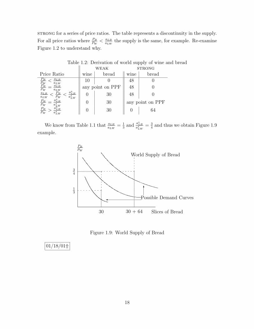
strong for a series of price ratios. The table represents a discontinuity in the supply.
For all price ratios where PB
PW< aLB
aLWthe supply is the same, for example. Re-examine
Figure 1.2 to understand why.
Table 1.2: Derivation of world supply of wine and breadweak strong
Price Ratio wine bread wine breadPB
PW< aLB
aLW10 0 48 0
PB
PW= aLB
aLWany point on PPF 48 0
aLB
aLW< PB
PW<
a?LB
a?LW
0 30 48 0PB
PW=
a?LB
a?LW
0 30 any point on PPFPB
PW>
a?LB
a?LW
0 30 0 64
We know from Table 1.1 that aLB
aLW= 1
3and
a?LB
a?LW
= 34
and thus we obtain Figure 1.9
example.
...............
..................... ...............................
PB
PW
Slices of Bread
13
34
30 30 + 64
World Supply of Bread
Possible Demand Curves
6
�
Figure 1.9: World Supply of Bread
01/18/01⇑
18

1.3.2 Wages
01/23/01⇓ Since there is no other factor, and we will assume therefore, that there
are no profits, workers earn the value of their labor. Let us say the demand is such
that the equilibrium price of bread and wine is 2 thirds ( PB
PW= 2
3). To make this math
easy we will assume that the price of bread is $2 a slice and the price of wine is $3 a
glass. Since it takes one third of a unit of labor to produce one slice of bread, each
unit of labor in weak earns $6. Each unit of labor in strong earns $12. Note that
strong is 1 and 1/3 as productive as weak in bread and 3 times as productive as
weak in wine, and it wages end up, in between, at 2 times as large as the wages in
weak.
Note, that at these prices the cost to weak of producing bread is $2 a slice
(given by the prices), the cost of producing wine would be $6, the cost to strong
of producing wine is $3 (given by prices) and the cost of producing bread would be
$4. It appears therefore, that each country sells the good that it can produce the
cheapest. This is, of course true, but is the result of trade, not the cause of it. The
relative wages between the counties is a product of trade.
This is the Ricardian Trade Model.
1.3.3 False Views of Trade
• Free Trade is beneficial only if your country is strong enough to stand up to
foreign competition [mistaking absolute advantage.] for comparative advantage.
• Foreign Competition is unfair and hurts labor in countries with higher wages
when it is based on low wages. (US is hurt in US/Mexico trade, for exam-
ple.)[Ans: It is cheaper to produce the good of your speciality and trade it for
the other.]
• Trade exploits a country and makes it worse off if its workers receive much
lower wages than workers in other nations. (Mexico is hurt in US/Mexico trade)
[strong gains more than weak, but weak gains compared to no trade.]
01/23/01⇑
19

Chapter 2
Specific Factors Model
2.1 Introduction
The Ricardian model of trade 01/23/01b⇓ is a nice simple model for showing the
gains to trade and even the affect of trade on relative wages between participating
countries. We know, however, that the gains from trade are not distributed evenly
among all owners of factors in an economy (where owners of factors might include
owners of labor, land or capital). This has very important implications for the political
economy of trade. In this section we develop a model of production and trade in which
there are three factors in the economy. The model of trade is essentially identical to
that in the previous section where we had a concave production possibility frontier.
However, we will be able to trace backwards the impact of trade on the relative wages
of all factors in the economy.
2.2 Graphical Representation
We begin with an economy in which there is labor (L), capital (K) and land (T ) (think
of territory[T]). Two goods are produced; Manufactures and Food. Manufactures
requires labor and capital and food requires labor and land. It should be clear that
the result of absolute specialization that we obtained with the Ricardian is unlikely to
occur with this model because specialization in one product would leave either land
or capital entirely unused.
The essential addition of this model is that capital cannot be used to produce
food and land cannot be used to produce manufactures. Labor can be used in either
20

allocation. There is a fixed supply of labor, capital and land, however all land will be
used in food and all capital in manufactures.
QM = QM(K, LM) (2.1)
QF = QF (T, LF ) (2.2)
LM + LF = L (2.3)
Figure 2.1 introduces the 4 quadrant diagram and shows the constraint for the
allocation of labor. The labor allocation frontier is very simple, there is a one for one
trade-off between sectors in the allocation of labor.
6
?
� - QM
QF
LM
LF @@
@@
@@
@@
@@
L
L
III
III IV
Slope = -1
Figure 2.1: PPF with Specific Factors: Labor Allocation
Figure 2.2 introduces the production functions QM = QM(K, LM) and QF =
QF (T, LF ) in quadrant IV and II respectively. The functions represent the diminishing
marginal productivity of labor (diminishing returns to labor) in each sector.
Question 3 Why does the curve representing the function QF = QF (T, LF ) represent
declining marginal productivity of labor?
21

6
?
� - QM
QF
LM
LF @@
@@
@@
@@
@@
L
L
III
IIIIV
j jjj
Figure 2.2: PPF with Specific Factors: Deriving the PPF
Now we can find the quantity of food and manufactures produced for any point
along the labor allocation frontier. Plotting these quantities in the first quadrant
gives us the points from which we will draw the production possibility frontier (see
Figure 2.2.)
The quantity of food and manufactures actually produced will depend on the
prices faced by the economy. This is exactly the same exercise as that shown in
Figure 1.3. We assume a particular ratio of prices and represent this as PM
PF. This
gives us the quantity of food and manufactures and we can trace this back to the
labor allocation frontier to see how much labor is used in each sector.
Alternatively, we can obtain the same result by saying that labor moves between
sectors until the wage rate is the same in each sector. The wage in any sector will
be equal to the marginal physical product of labor times the price of the good being
produced. Note that the marginal physical product of labor is very often called simply
the marginal product of labor. I use the term “physical” to remind us that this is a
measurement in units of output, not value. The marginal value product of labor is
the marginal physical product times the price. Hereafter, the term MPL refers to the
22
6
?
� - QM
QF
LM
LF @@
@@
@@
@@
@@
L
L
III
IIIIV
PPF.............................................................................................
...
...
...
...
...
...
...
...
...
...
...
...
...................................................
LM |PM
PF
LF |PM
PF
QQk
Slope −PM
PF
Slope −MPLF
MPLM
�
�HH
HHHj
Figure 2.3: PPF with Specific Factors: Distribution of Labor
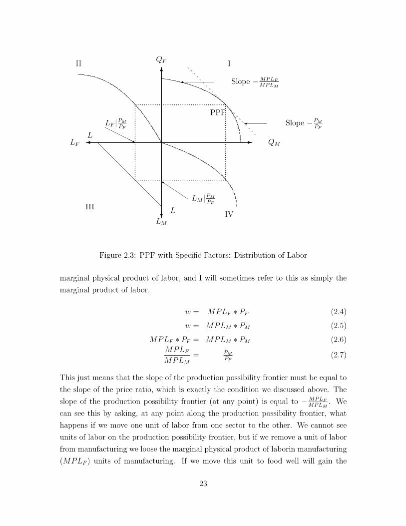
marginal physical product of labor, and I will sometimes refer to this as simply the
marginal product of labor.
w = MPLF ∗ PF (2.4)
w = MPLM ∗ PM (2.5)
MPLF ∗ PF = MPLM ∗ PM (2.6)
MPLF
MPLM
= PM
PF(2.7)
This just means that the slope of the production possibility frontier must be equal to
the slope of the price ratio, which is exactly the condition we discussed above. The
slope of the production possibility frontier (at any point) is equal to −MPLF
MPLM. We
can see this by asking, at any point along the production possibility frontier, what
happens if we move one unit of labor from one sector to the other. We cannot see
units of labor on the production possibility frontier, but if we remove a unit of labor
from manufacturing we loose the marginal physical product of laborin manufacturing
(MPLF ) units of manufacturing. If we move this unit to food well will gain the
23

marginal physical product of labor in food (MPLF ) units of food. The rise is−MPLF
and the run is MPLM , thus the slope is −MPLF
MPLM.
If, MPLF ∗ PF > MPLM ∗ PM then the wage rate in the food sector is higher
than the wage rate in the manufactures sector and labor will leave the food sector
and migrate to the manufactures sector.
Question 4 As labor leaves a sector the marginal physical product of labor rises or
falls?
As labor leaves a sector the marginal physical product of labor in that sector will rise
(the definition of diminishing returns to labor) and it will fall in the sector which is
attracting labor. So this migration will equalize the wages.
2.3 Changes in the Price Ratio
2.3.1 Equi-proportional changes in prices
Question 5 What happens to this equilibrium when the price of both food and man-
ufactures increases by 10%
• The price ratio is unchanged so the equilibrium allocation of labor cannot change
• But what about wages?
• Even though nominal wages will rise, the real wage is unaffected, in this model
with only two goods. This does not depend on any qualities of the income effect.
• If there was a third good whose price did not change, then we could have an
income effect.
2.3.2 Differential changes in prices
01/30/01⇓ As the previous exercise demonstrates, it is important to examine, not
just the changes in wages, but the changes in the purchasing power of these wages.
Thus we are not concerned with nominal wages but real wages. To do this we will
examine the wage in terms of the number of units of both food and manufacture that
can be purchased with the wage. If we observe that the wage of labor can purchase
both more manufactures and more food (if it is used to buy only one or the other
good) then it is clear that laborers are better off.
24

2.3.2.1 Earnings of Capital
We start with what should be a clear cut situation. If the price of manufactures rises
and the price of food remains the same we would be surprised if the owners of capital
were not better off absolutely. What are the earnings of capital? We will call the
profits of capitalists πK , the wage paid per unit labor w and the profits of landowners
πT .
πK = PMQM − LMw Revenues - Wages paid (2.8a)
πK = PMQM − LMMPLMPM From determination of wages (2.8b)πk
PM
= QM − LMMPLM Profits in units of manufacturing (2.8c)
πk
PM
= LM
(QM
LM−MPLM
)Algebraic manipulation (2.8d)
πk
PM
= LM (APLM −MPLM) (2.8e)
The profits of the capitalist (in terms of the number of units of manufacturing
that he could buy with his profits) can be represented as the quantity of labor used
times the difference between the average product of labor and the marginal physical
product of labor.This makes intuitive sense because the marginal product of labor
determines the wage that must be paid to the last worker hired (and therefore to
all the workers) and the average product of labor determines the productivity of the
work force as a whole. The capitalist only makes profits if the APLM is greater than
the MPLM . When is this true? Here it helps to examine the production function for
manufactures again.
Figure 2.4 shows how one would graphically determine the APLM and the MPLM
with a standard production function. Convince yourself that the slope of the marginal
product will always be less than the slope of the average product. We therefore obtain
the values of APLM and MPLM shown in Figure 2.5.
Figure 2.5 shows that the average product is greater than the marginal product,
and therefore the capitalist earns profits. Additionally, as the use of labor increases,
the difference between the average and marginal product increases. Thus as the use
of labor increases the profits of the capitalist increase. We know that the impact
of a change in prices favoring the manufacturing sector is that labor shifts from the
food sector to the manufacturing sector. Returning to Equation 2.8e we can see that
25

LM
QM
QM(K, LM)
.......................................
Slope = MPLM
?
Slope = APLM�
Figure 2.4: Finding the APLM and MPLM with diminishing returns to labor
as LM increases, the profits in terms of units of manufacturing is increasing both
because LM increases and because APLM − MPLM is increasing. 01/23/01b⇑ To
show that the capitalist is absolutely better off we need to show that he can also
purchase more food with his profits. To do this we take his profits measured in terms
of units of manufacturing, multiply by the price of manufactured goods (to get a
money measure) and divide by the price of food (to get the number of units of food).
πk
PF
= LMPM
PF
(APLM −MPLM) (2.9)
Equation 2.9 represents the units of food the capitalist could purchase with the
profits earned in manufacturing. As the price of manufacturing rises relative to food
this amount goes up by even more than the profits measured in terms of manufac-
turing. Thus the capitalist can buy more of everything when the relative price of
manufacturing increases.
2.3.2.1.1 Earnings of Landowners It should be clear that the owners of land
will do worse. We pick up the from Equation 2.8e and represent the number of units
of food that the profits of landowners can purchase as seen in Equation 2.10.
πT
PF
= LF (APLF −MPLF ) (2.10)
26

LM
MPLM
APLM
ee
ee
ee
ee
ee
e
APLM
MPLM
...
...
...
...
...
...
...
...
...
...
...
...
...
...
...
...
...
...
...
...
...
...
...
.
L1 L2
Figure 2.5: APLM and MPLM with diminishing returns to labor
We know that labor is shifting away from the food sector when the price of manufac-
turing increases. Thus LT and APLT −MPLT are both falling and the profits of the
landowners is clearly falling. If it is falling in terms of food (which has become rela-
tively cheaper) then it must be falling in terms of manufacturing (which has become
relatively more expensive).
2.3.2.1.2 Earnings of Labor The earnings of each laborer is just his wage.
The number of units of manufacturing that can be purchased with that wage is the
marginal physical product of labor in manufacturing, and the number of units of food
that can be purchased is the marginal physical product of labor in food production.
w = MPLMPM (2.11)w
PM
= MPLM (2.12)
w = MPLF PF (2.13)w
PF
= MPLF (2.14)
Since labor is moving from the food to the manufacturing sector the marginal products
are changing.
Question 6 Why does labor migrate from food to manufacturing when the price ratio
changes, and why do the marginal products change?
The marginal product of labor in the manufacturing sector is falling and the marginal
product of labor in the food sector is rising. Thus labor can purchase less manufac-
27

tures and more food. We don’t know if they are better or worse off. This depends on
how much they like manufacturing compared to food.
2.3.3 Graphical Representation of Changes in Wages
LM LF
wage
- �
MPLF PFMPLMPM
w
LM
Figure 2.6: Graphical Representation of Equilibrium in Wages
Figure 2.6 shows a graphical representation of the determination of the equilibrium
wage rate. As labor is shifted from one industry to another the marginal physical
products of labor are changing. The equilibrium allocation of labor is achieved where
the wage rates are the same across industries.
LM LF
wage
- �
MPLF PFMPLMPM
w
LM
...
...
...
..
L2M
w2
MPLMP 2M
...................................w?
Figure 2.7: Graphical Representation of Change in Relative prices
Figure 2.7 represents the determination of a new equilibrium when the price of
manufactures rises. When the price of manufactures rises this causes the marginal
28

value product curve to shift upwards. Note that it does not shift upwards uniformly
because the change in prices causes a larger shift when the marginal physical product
of labor is larger. It is a multiplicative upwards shift, not an additive upwards shift. If
there was no reallocation of labor the new wage would be the intersection shown by the
intersection of LM and w?. However, with reallocation of labor we get an intersection
at L2M and w2. Note that the reallocation cause the wage in manufacturing to fall
and the wage in food to rise.
LM
MPLM
MPLM
ee
ee
ee
ee
ee
e
Income of capitalists
Wages
��
�/
������
..................................L1
M L2M
Increase in capitalist income�
��=
Figure 2.8: Graphical Representation of Capitalist Income
Figure 2.8 shows that capital income can be represented on the marginal product
of labor curve. It is the area above the marginal product of labor and below the
curve. As labor shifts out this area unambiguously increases, as labor shifts in this
area unambiguously decreases. Note that we cannot make conclusions about wages
because the area shown is the total wage bill, not the actual wage.
2.4 Implication of the Model
Trade benefits the factor that is specific to the export sector of each country but hurts
the factor specific to the import-competing sectors with ambiguous effects on mobile
factors.
29

2.5 Political Economy Considerations
Question 7 The textbook states that there are three main reasons why economists do
not stress the income distribution effects of trade. What are these?
• Income distribution effects are not specific to international trade.
• It is always better to allow trade and compensate those who are hurt than to
prohibit trade.
• Those who stand to lose from increased trade are typically better organized
than those who stand to gain.
01/30/01⇑
30

Chapter 3
Factor Proportions Model
(Heckscher–Ohlin Model)
3.1 Introduction
In this model all factors are mobile but specialization comes from the 02/01/01⇓relative proportion of factors in the economy. Two goods are produced and each is
relatively intensive in its use of one of two factors in the economy.
We will be considering an economy that produces food (F ) and cloth (C) with
land (T ) and labor (L). We assume that cloth is labor intensive and that food is land
intensive. This does not mean that food production does not require labor, but that
it requires proportionately more land than does cloth production.
3.2 Fixed Coefficients Model
In this simplified view of the of the economy food and cloth are produced with fixed
ratios of the two inputs.
The fixed coefficients are defined as follows:aTC Units of land required to produce one unit of cloth
aLC Units of labor required to produce one unit of cloth
aTF Units of land required to produce one unit of food
aLF Units of labor required to produce one unit of food
31

The assumption of factor intensity is represented by the inequality in Equation 3.1
aLC
aTC
>aLF
aTF
(3.1)
Or equivalentlyaLC
aLF
>aTC
aTF
(3.2)
We know that the total amount of labor or land used in the economy cannot
exceed L or T , the endowment of labor and land. Note that aLCQC (where QC is the
quantity of cloth) is just LC , and we obtain Equation 3.4 and Equation 3.3.
aLCQC + aLF QF ≤ L (3.3)
aTCQC + aTF QF ≤ T (3.4)
These can be rewritten as:
QF ≤ L
aLF
−(
aLC
aLF
)QC (3.5)
QF ≤ T
aTF
−(
aTC
aTF
)QC (3.6)
These rewritten equations can in turn be graphed in QC and QF space to create the
production possibility frontier of this economy.
JJJJJJJJJJJJ
QC
QF
LaLF
TaTF
LaLC
TaTC
Labor Constraint
Land Constraint1
2
3
4Q
SSSSS
�
�
PPF�����
Figure 3.1: Deriving the PPF with Fixed Coefficients
32

The labor constraint represented in Figure 3.1 is Equation 3.5 and the land con-
straint is Equation 3.6. Note that the slopes of the two constraints are aLC
aLFand aTC
aTF
for labor and land respectively. We know from the assumption on factor intensity as
seen in Equation 3.2 that the slope of the labor constraint is steeper than the slope
of the land constraint.
The Labor constraint, for example, represents the set of points for which all labor
is allocated to the production of either cloth or food. Every point below the constraint
is possible, but leave labor idle. Points above the constraint are not possible. Thus,
point 1 in Figure 3.1 represents the set of cloth, food output combinations that leave
both land and labor idle. Point 2 represents outputs for which labor would be idle,
but there is insufficient land, and point 3 points for which land is idle but there is
insufficient labor. Point 2 and 3 are therefore not possible. Clearly point 4 is not
possible. The production possibility frontier is therefore defined by the area interior
to both the labor and land constraint.
We chose the intercepts for both lines so that there would be an intersection. This
is not a necessary outcome of the assumptions that we have made so far. However,
if this were not true we would return to the Ricardian model of chapter 1. Let us
examine the impact of increasing the quantity of labor available for production in
this economy.
JJJJJJJJJJJJ
QC
QF
LaLF
TaTF
LaLC
TaTC
L?
aLF
New Labor Constraint
New PPF
QSSSSS
�
�
L?
aLC
Figure 3.2: Fixed Coefficients PPF, increasing Labor Supply
Figure 3.2 shows the effect of an increase in labor supply on the production possi-
bility frontier. The intercepts for the labor constraint shift out, though the slope does
33

not change. This pushes the production possibility frontier outwards, but only in the
direction of increased cloth. It is possible that the labor constraint would shift out so
much that it would no longer be a binding constraint. In this case the land constraint
would be the only effective constraint. This problem returns to the Ricardian model
of chapter 1.
3.2.1 Impact of Prices
With the Ricardian model Again we start with a small country assumption, where
the country accepts a set of prices given exogenously from outside. The impact wide
ranges of prices caused no changes in the production decisions of the economy. In
this model we have a similar impact. When the slope of the price line is flatter than
the slope of the labor constraint we observe production of food only (for example,
price ratio 1 in Figure 3.3). For all slopes that are steeper than the labor constraint
but flatter than the land constraint we observe exactly the same output (C and
F in Figure 3.3.) Price ratios 2 and 3 are examples of price ratios that give this
intermediate income. When the slope of the price ratio is steeper than the land
constraint we observe production of only cloth (price ratio 4 in Figure 3.3.)
QC
QF
PPPPPPPTTTTT
1
23
41,2,3 and 4 are
sample price ratios
...
...
...
...
...
...........................F
C
Figure 3.3: Impact of various price ratios on production decision
Thus, for a wide range of prices we observe no change in the productive output
of the economy. Since outputs are not changing, neither is the allocation of land and
labor in the economy. Thus it would appear that prices (so long as they are within
the intermediate range) have no impact on the economy.
34

3.2.2 Prices and Factor Incomes
In fact, prices have a very important impact on the economy and this is seen in the
income of the two factors land and labor. We reintroduce the following notation: PC
is the price of cloth; PF is the price of food; w is the wage of labor and r is the rental
for land.
We assume perfect competition in the supply of each factor and therefore that
there are not profits in the production of either good. Anything earned in the pro-
duction of either good is paid to labor and land. This gives us Equation 3.7 and
Equation 3.8.
PC = aLCw = aTCr (3.7)
PF = aLF w = aTF r (3.8)
Equation 3.7 and Equation 3.8 state that all the proceeds the sale of cloth and food
respectively are consumed by the wage and rent paid to the labor and land used in
production.
These equations can be rewritten so that they can be graphed in r,w space as in
Figure 3.3.
w
r
@@
@@
@@
@@
@@
HHHHHHHHHHHHH.................................
w?
r?
PC
aTC
PF
aTF
PC
aLC
PF
aLF
Figure 3.4: Equilibrium in the wage and rental market for factors
Verify for yourself that the slope of the perfect competition in the production of
cloth restriction (Equation 3.7) is steeper than the slope of the perfect competition
in food restriction (Equation 3.8).
35

All points above the perfect competition in cloth restriction represent points where
the final price of a unit of cloth is less than the cost of production. Points below the
restriction represent points where the final price is less than cost of the inputs.
Production in both food and cloth must be along the perfect competition restric-
tion and therefore the equilibrium in this economy is the point where wages are w?
and the rent is r?. [include a note eventually about how the economy moves towards
equilibrium if it starts away from the equilibrium].
02/05/01⇓ The importance of prices is shown in Figure 3.5.
w
r
@@
@@
@@
@@
@@
HHHHHHHHHHHHH.................................
w1
r1
PC
aTC
PF
aTF
PC
aLC
PF
aLF
P 2C
aTC
......................................
w2
r2
P 2C
aLC
Figure 3.5: Prices of Cloth and Food and the Wage and Rent Equilibrium
When the price of cloth increases we observe a new equilibrium. The wage shifts
from w1 to w2 and the rent shifts from r1 to r2. While the wage increases the rent
falls. This is because cloth is labor intensive. Thus prices have a very important
impact for owners of the factors of production.
02/01/01⇑ This result is suggestive of the Stolper–Samuelson Theorem which
states that:
Theorem 1 (Stolper-Samuelson Theorem) A rise in the relative price of a good
will lead to a more than proportional rise in the return of the factor used intensively
in the favored sector, and a decline in the return to the other factor
36

3.3 Numerical Example, Magnification Effect in
the Stolper–Samuelson Theorem
We will work with the case of fixed coefficients, a result of Leontief production func-
tions in the two sectors (which we will call X and Y ). We have two factors, skilled
and unskilled labor (denoted by H and L, respectively), which are used in different
ratios in the two sectors. Assume that prices are exogenous. We can then calculate
the wages (for skilled and unskilled labor) that would have to result if zero-profit
conditions were to be maintained.
Assume that we have the following conditions:
PX = 4 and PY = 8
aHX = 4 and aHY = 4
aLX = 2 and aLY = 8
In addition to prices, we also know the number of units of factor (H or L) required
to produce one unit of a good (X or Y ). The value of aHX , for example, tells us the
number of units of skilled labor required to produce a unit of good X (the answer, in
this case, being 4).
We can verify that sector X is the skill-intensive sector. Note that the ratio of
skilled-to-unskilled labor in sector X is higher than that in sector Y .
aHX
aLX
=4
2= 2 and
aHY
aLY
=4
8=
1
2
Perfect competition implies that we have zero profits in both sectors. The value
of the output in each sector has to be completely exhausted by payments made to
different factors of production Since we have two factors, skilled and unskilled labor,
with wages (wH and wL, respectively) being their costs of use, we get the following
zero-profit conditions:
for sector X : PX = wHaHX + wLaLX
for sector Y : PY = wHaHY + wLaLY
37

Rewriting these equations, we get:
for sector X : wH = (1
aHX
)PX − (aLX
aHX
)wL
for sector Y : wH = (1
aHY
)PY − (aLY
aHY
)wL
Now, fill in what we know about the variables:
for sector X : wH = (1
4)4− (
2
4)wL = 1− (
1
2)wL
for sector Y : wH = (1
4)8− (
8
4)wL = 2− 2wL
We now have two equations with two unknowns, wH and wL. We can easily solve
this system of equations:
1− (1
2)wL = 2− 2wL
(3
2)wL = 1
=⇒ wL =2
3
and wH = 1− (1
2)(
2
3) = 1− 1
3=
2
3
Now suppose that the price of the unskilled labor intensive good, Y , declines from
$8 to $6. An immediate effect of this is the change in the zero-profit condition for
sector Y (since the value of the output has gone down, the right hand side in the
zero-profit condition above also has to go down for given technology coefficients to
maintain equality). Since price of the other good, X, hasn’t changed, the zero-profit
relation in that sector does not change. So, we have:
for sector X : wH = 1− (1
2)wL
for sector Y : wH = (1
aHY
)PY − (aLY
aHY
)wL = (1
4)6− (
8
4)wL = (
3
2)− 2wL
Once again, we equate the two zero-profit conditions and get the following:
38

1− (1
2)wL = (
3
2)− 2wL
(2− 1
2)wL = (
3
2− 1)
(3
2)wL =
1
2
=⇒ wL =1
3
and wH = 1− (1
2)(
1
3) = 1− 1
6=
5
6
Let us summarize the changes:
• The price of good Y declined from $8 to $6. Since PX hasn’t changed, we now
have a decrease in the relative price of Y , (PY
PX), from (2) to (3
2). This is a
decrease of 25 percent.
• The return to unskilled labor, wL, declined from 23
to 13
(a decline of 50 percent).
The return to skilled labor, wH , increased from 23
to 56. Note that the percentage
fall in the wages of unskilled labor is higher than the percentage fall in the price
of the unskilled labor-intensive good.
This confirms the Stolper-Samuelson Theorem
3.4 Variable Coefficients
Here we will examine an economy that produces two goods X and Y using labor (L)
and capital (K).
The marginal rate of technical substitution (MRTS) which is occasionally referred
to as the rate of technical substitution (RTS) is the units of labor (for example)
required to compensate for the loss of a unit of capital holding output constant.
Question 8 Why is the isoquant convex to the origin?
Diminishing marginal rate of technical substitution. Think of preference of bundles
over extremes.
We will refer to the capital labor ratio as k, and this can be represented as a ray
from the origin.
39

L
K
Output 1
Output 2
Output 3
Slope is MRTS��
������
Figure 3.6: Isoquants
Constant returns to scale (CRS) justifies looking at the unit isoquant and ignoring
issues of scale.
The isocost frontier is a collection of points which represents exactly the same
total input cost. The slope of this frontier is defined by the ratio of the wage to the
rental rate (r is the per unit cost of capital, referred to as the rental rate). In other
words, this is the market exchange of a unit of capital for a unit of labor.
We want to produce a unit of output at the lowest cost, so we search for the lowest
isocost frontier that will achieve a unit of output. This is obtained where the slope of
the marginal rate of technical substitution is equal to the ratio of factor costs. This
then defines the capital labor ratio (k) for the production of that good. Because of
our assumption about constant returns to scale this ratio will hold for any given wage
rent ratio no matter what the scale of production.
Definition 3 (Strong Factor Intensity) In a two factor, two good economy strong
factor intensity implies that for all wage rent ratios, the ratio of capital to labor used in
the production of X is greater than the ratio of capital to labor used in the production
of Y . In this case X is strongly more intensive in the use of capital than Y
Note that the constant returns to scale is not enough to guarantee strong factor
intensity. We can see strong factor intensity in Figure 3.10.
40

L
K k1
k2
k3...............................
...............................
...............................
MRTS is constantas output expands�
��
���
��
��
�
��
��
��
�+
Figure 3.7: Isoquants and Constant Returns to Scale
3.4.1 Lerner Diagram
Now the Lerner diagram shown in Figure 3.11 represents an equilibrium. The ratio
of the price of good X to the price of good Y is exactly the right amount to insure
that the cost of producing QX and Q?Y = QX · PX
PYis exactly the same. But we can
see why this was true by assuming one or the other
3.4.1.1 Fix factor prices, derive goods prices
Find the unit isoquant for good X (where quantity of X is Q1X) and its tangency
with the isocost frontier. Then find the greatest isoquant for the production of Y
that touches that unit isoquant. This gives us the number of units of Y that can be
exchanged for one unit of X when the costs of production are identical, and therefore
sets the price ratio.
3.4.1.1.1 Fix goods prices, derive factor prices If we know the price ratio
we know both QX and Q?Y = QX · PX
PY. Graph both isoquants and find the unique
wage rent ratio isocost frontier that is tangent to both lines. This fixes the wr.
3.4.2 Impact of Changing Prices
02/08/01⇓02/05/01⇑
41

L
K
@@
@@
@@
@@
@
@@
@@
@@
@
ll
ll
ll
ll
ll
ll
ll
l
Slope = −wr��������)
� PPPPPPi
Unit Isoquant�
Figure 3.8: The unit isoquant and isocost frontiers
L
K
Unit isoquant...........................................
........
........
........
........
........
(wr
)0
(wr
)1
k0
k1
Figure 3.9: Wage, rent ratios and the capital-labor ratio
Impact of change in prices (moving from points 0 to points 1). The relative price
of Y increases. This is the labor intensive good. This lead to an increase in the wage
compared to the rent. This in turn leads to an increase in the capital labor ratio for
both X and Y.
The wage increases relative to the rent, but are laborers better off? Recall that in
the Specific Factors Model the owner of the favored fixed factor gained unambiguously
but the owner of the other factor lost unambiguously. This seems like an extreme
result and we would not necessarily expect such result when both factors are mobile.
However, this is exactly what we get.
The important thing to note is that the capital labor ratio has changed in each
42

wr
k = KL
��������������
�������������
kX
kY
Figure 3.10: Relationship between wr
and k
L
K
@@
@@
@@
@@
@
kX
kY
Q1X
Q?Y = Q1
X · PY
PXslope = −wr
6
Isocost frontier������9
Figure 3.11: The Lerner Diagram
sector. We are assuming, as we did in the specific factor model, that workers are paid
the marginal product of their labor and that capital is paid the marginal product of
capital. This is just an equilibrium condition.
Question 9 What is the difference between the statement : “factors are paid their
marginal value product”, and “workers are paid a fair wage,” or workers are paid
what they are worth?”
When the capital labor ratio changes this changes the marginal physical product of
labor and capital. When less workers are working with more machines, the additional
product of the marginal laborer increases. (We expect his average product to increase
as well.) In addition, the marginal physical product of capital should fall. This is all
43
L
KQ1
X
Q?YQ??
Y
(wr
)0 (
wr
)1
�
�
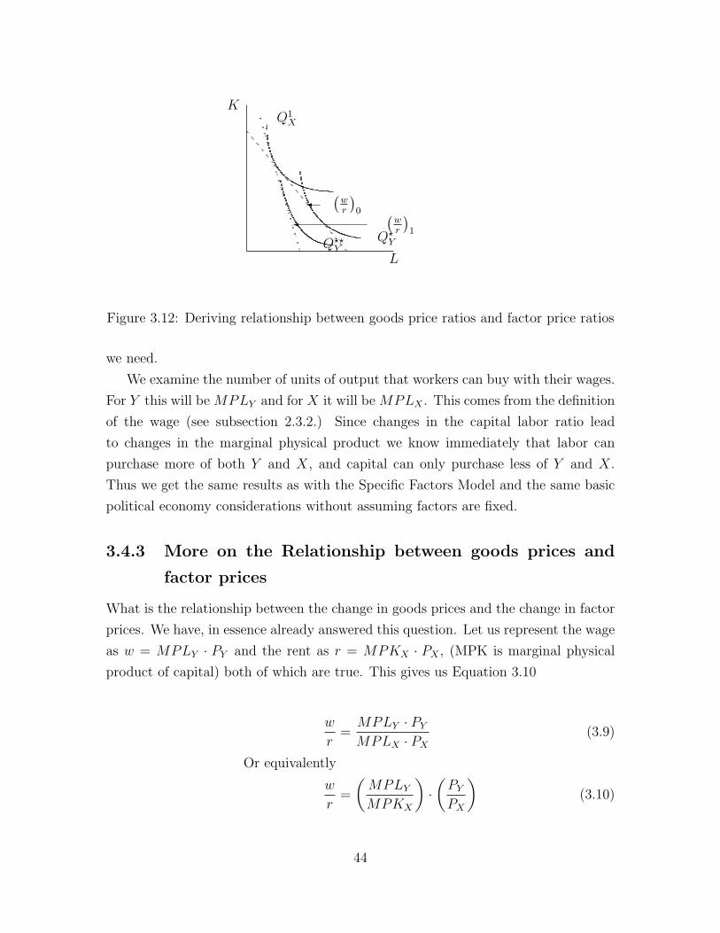
Figure 3.12: Deriving relationship between goods price ratios and factor price ratios
we need.
We examine the number of units of output that workers can buy with their wages.
For Y this will be MPLY and for X it will be MPLX . This comes from the definition
of the wage (see subsection 2.3.2.) Since changes in the capital labor ratio lead
to changes in the marginal physical product we know immediately that labor can
purchase more of both Y and X, and capital can only purchase less of Y and X.
Thus we get the same results as with the Specific Factors Model and the same basic
political economy considerations without assuming factors are fixed.
3.4.3 More on the Relationship between goods prices and
factor prices
What is the relationship between the change in goods prices and the change in factor
prices. We have, in essence already answered this question. Let us represent the wage
as w = MPLY · PY and the rent as r = MPKX · PX , (MPK is marginal physical
product of capital) both of which are true. This gives us Equation 3.10
w
r=
MPLY · PY
MPLX · PX
(3.9)
Or equivalently
w
r=
(MPLY
MPKX
)·(
PY
PX
)(3.10)
44

wr
PY
PX
Figure 3.13: The relationship between goods price ratios and factor price ratios
We know that PY
PXis increasing, furthermore we know that MPLY
MPKXis also increasing
since the marginal product of labor is rising in both sectors and the marginal physical
product of capital is falling in both sectors. Thus the increase in wr
is proportionately
greater than the increase in PY
PX.
3.5 Stolper–Samuelson
Theorem 2 (Stolper-Samuelson Theorem) A rise in the relative price of a good
will lead to a more than proportional rise in the return of the factor used intensively
in the favored sector, and a decline in the return to the other factor
3.6 Capital-Labor Ratio and Specialization
If we look at the case where the capital labor ratio is given in the economy we can
see some interesting patterns already. In Figure 3.15 the capital labor ratio in the
economy is given. This gives us a range of goods prices (A to B) for which the
economy will produce some of each good.
02/20/01⇓
45

PY
PX
wr
KL
##
##
##
##
##
##
##
��
��
��
��
��
��
��
�
ky kx
(PY
PX
)1
(PY
PX
)0
k0Y k0
xk1Y k1
X
Figure 3.14: Prices, wage-rent ratios and capital labor ratios
3.7 Allocation of Resources to Production
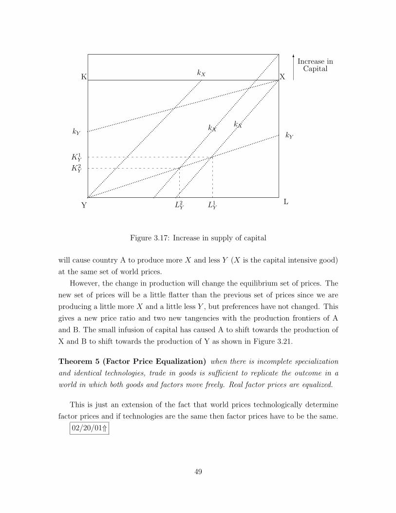
02/09/01⇑ When the supply of capital increases in the economy we get a very strong
result. Figure 3.17 shows the impact of an increase in the supply of capital. The y
axis shifts upwards and we draw a new capital labor ratio from the point of view of
the production of X.
Note that the use of capital in the production of X increases. This is not surprising
since X is the capital intensive good. However, note that the increase in the use of
capital X is greater than the additional capital added to the economy. In addition
the use of labor expands. X gets more than its share of capital and uses additional
labor as well.
Theorem 3 (Rybczynski Theorem) At constant relative goods prices, a rise in
the aggregate endowment of one factor will lead to a more than proportional expansion
of the output in the sector which uses that factor intensively, and an absolute decline
of the other good. [as long as the economy continues to be incompletely specialized as
its factor endowments change].
46

PY
PX
wr
KL
##
##
##
##
##
##
##
��
��
��
��
��
��
��
�
ky kx
K̄L̄A B
Figure 3.15: Prices, wage-rent ratios and capital labor ratios
K̄
L̄=
KX + KY
L̄
=KX · LX
LX+ KY · LY
LY
L̄
=kX
(LX
L̄
)+ kY
(LY
L̄
)=kX
(LX
L̄
)+ kY
(L̄− LX
L̄
)=kX
(LX
L̄
)+ kY − kY
(LX
L̄
)K̄
L̄= (kX − kY )
(LX
L̄
)+ kY (3.11)
If the capital labor endowment ratio increases, the only way to balance Equation 3.11
is to increase the use of labor in the factor that uses capital more intensively.
3.8 Biased Expansion of the PPF
The Rybczynski theorem can also be seen in what we call the biased expansion of the
production possibility frontier. Here we start with the production possibility frontier
and show what happens if we increase the quantity of one factor or another.
In Figure 3.18 we generate an expanded production possibility frontier on the basis
47

Y
XK
L.............................................................................................
..............
..............
..............
..............
..............
..............
..............
............
........................................................................................
.............................................................................................................kY
kX
kY
kX-Increasing Labor in Y
IncreasingCapital in Y
6
LY
KY
Figure 3.16: Allocation of resources in Heckscher–Ohlin economy
of the following. First, as seen in Figure 3.17, when the supply of capital increases
and the price of the final goods stay the same we get more X produced and less
Y . We draw this on Figure 3.18 by showing that the point on the new production
possibility frontier that is tangent to the old price line is to the right and below the
previous point.
This process (repeated for each possible price) gives us the production possibility
frontier shown in Figure 3.19. Note that this production possibility frontier is biased
towards the production of X (because X is the capital intensive good and we have
more capital than before).
Theorem 4 (Heckscher–Ohlin Theorem) A country has a production bias to-
wards, and hence will tend to export, that good which uses intensively the factor that
is relatively abundant in that country
Figure 3.20 begins with two identical countries. They each have the same PPF
and consumer preferences so they produce at exactly the same point, consume at
exactly the same point and there is no trade. We add a small amount of capital to
economy A. This causes a biased expansion in the PPF of country A. We know this
48
Y
XK
L.............................................................................................
..............
..............
..............
..............
..............
..............
..............
............
........................................................................................
.............................................................................................................kY
kX
kY
kXkX
L2Y L1
Y
K1Y
..........................................................................................................
6Increase inCapital
K2Y
Figure 3.17: Increase in supply of capital
will cause country A to produce more X and less Y (X is the capital intensive good)
at the same set of world prices.
However, the change in production will change the equilibrium set of prices. The
new set of prices will be a little flatter than the previous set of prices since we are
producing a little more X and a little less Y , but preferences have not changed. This
gives a new price ratio and two new tangencies with the production frontiers of A
and B. The small infusion of capital has caused A to shift towards the production of
X and B to shift towards the production of Y as shown in Figure 3.21.
Theorem 5 (Factor Price Equalization) when there is incomplete specialization
and identical technologies, trade in goods is sufficient to replicate the outcome in a
world in which both goods and factors move freely. Real factor prices are equalized.
This is just an extension of the fact that world prices technologically determine
factor prices and if technologies are the same then factor prices have to be the same.
02/20/01⇑
49

X
Y
...............................................................
Slope is PX
PY���+
X1
Y1
...............................................................
Y2
X2
Figure 3.18: Biased Expansion of the PPF: I
X
Y
PPF(1)
PPF(2)
Figure 3.19: Biased Expansion of the PPF: II
50

X
Y
PPF forA and B
- New PPF for A�
........
........
........
........
........
........
........
........
........
........
......
..........
..........
..........
..........
..........
..........
..........
..........
..........
.?
Change in production (for A)towards X
Figure 3.20: Two countries begin identical: Add small amount of capital to A’sresources: I
X
Y
PPF(B) PPF (A)
................................................................................................
........................................................................................................
........
........
........
........
........
........
........
........
........
......
-
Change in equilibrium price ratio-.....
..........
..........
..........
..........
..........
..........
..........
..........
....
........
........
........
........
........
........
........
........
........
........
......�
?
B shifts towards Y
A shifts towards X
Figure 3.21: Two countries begin identical: Add small amount of capital to A’sresources: II
51

02/20/01⇓ Questions from Magee (1989). Note; think of the Ricardo–Viner–
Cairnes model, not as the one–factor Ricardian model that we discussed but as the
specific factors model in which both labor and capital are specific factors in each
sector. (The third, mobile factor does not matter, it can be anything.) Thus labor in
one sector does not move into another sector.
1. Assume trade hurts sector B and benefits sector A. Sector B is labor intensive
and sector A is capital intensive. Thus there are two sectors and 2 factors in
the Stolper–Samuelson setup, but 4 factors (labor A, labor B, capital A and
capital B) in the Ricardo–Viner–Cairnes setup.
(a) What coalition does Stolper–Samuelson suggest will form to support trade?
(b) What coalition does Stolper–Samuelson suggest will form to oppose trade?
(c) What coalition does Ricardo–Viner–Cairnes suggest will form to support
trade?
(d) What coalition does Ricardo–Viner–Cairnes suggest will form to oppose
trade?
2. Which of these two theories does the empirical evidence support?
3. Does the fact that trade negotiations (at the time of this paper) are always
short term, impact the expectation as to which theory is most likely to hold?
4. What impact, if any, could we expect from the transformation of trade negotia-
tions from short to long term (which is how it is done now as opposed to when
this paper was written)?
Questions from Wood (1997).
1. What is the puzzle that this paper posits and seeks to explain?
2. The paper states “Half the world’s population, and an even higher propor-
tion of the world’s unskilled workers, live in five low-income Asian countries:
Bangladesh, China, India, Indonesia and Pakistan. In the 1960’s and 1970’s, all
five countries were largely closed to trade, and thus their workers did not form
part of the effective world labor supply. By the mid–1980’s, these countries
were all opening to trade, led by Indonesia and China, with the South Asian
countries also making some progress.”
52
(a) What does this fact have to do with comparing the wage differentials and
the impact of trade in Latin American and East Asia?
3. The paper suggests that a Heckscher–Ohlin model with the addition of a third
factor such as land could explain the widening of the wage differential in Latin
America and its narrowing in East Asia.
(a) What are the key assumptions that would make the addition of this factor
have this impact?
(b) Does this appear to be likely?
4. What is the theory of skill-biased technical progress, or “skill-enhancing trade”?
(a) In what way does it violate the core assumptions of Heckscher–Ohlin?
(b) What evidence exists to back up this theory?
(c) What evidence exists to refute the theory?
3.9 Conclusions
• Trade is driven by differences in resource endowments
• Abundance of factors is relative, not absolute
• There are strong income distribution effects and strong predictions about the
direction of these impacts
• Benefits to factors do not depend on the sector in which a factor is employed
• The good that uses the relatively abundant factor intensively is traded and that
factor benefits.
• The good that uses the less abundant factor more intensively competes with
imports and that factor looses from trade.
02/22/01⇑
53

Chapter 4
Basic Trade Policy and Welfare
Analysis
4.1 Introduction
This chapter is covered in the textbook
4.2 Rent seeking activities with quotas and import
licenses
Consider first the results of an import-licensing mechanism when licenses
for imports of intermediate goods are allocated in proportion to firms’
capacities. . . . By investing in additional capacity, entrepreneurs devote
resources to compete for import licenses (Krueger, 1974, p. 292).
[L]icenses are allocated pro rata in proportion to the applications for those
licenses from importers-wholesalers. . . . In this case, competition for rents
occurs through entry into the industry with smaller-than-optimally sized
firms, and resources are used in that the same volume of imports could
be efficiently distributed with fewer inputs if firms were of optimal size
(Krueger, 1974, p. 292).
A third sort of licensing mechanism is less systematic in that government
officials decide on license allocations. Competition occurs to some extent
through both mechanisms already mentioned as businessmen base their
54

decisions on expected values. But, in addition, competition can also oc-
cur through allocating resources to influencing the probability, or expected
size, of license allocations. Some means of influencing the expected allo-
cation — trips to the capital city, locating the firm in the capital, and
so on — are straightforward. Others, including bribery, hiring relative of
officials or employing the officials themselves upon retirement, are less so.
In the former case, competition occurs through choice of travel, and so
on. In the latter case, government officials themselves receive part of the
bribes (Krueger, 1974, p. 292).
The above results are sufficient to indicate that, for any given level of
import restrictions, competitions among rent seekers is clearly inferior to
the tariff equivalent of the restrictions, in that there could be more food
consumed with no fewer imports under the latter case than the former.
To the extent that rent seeking is competitive, the welfare cost of import
restrictions is equal to the welfare cost of the tariff equivalent plus the
additional cost of rent-seeking activities Krueger (1974, p. 299).
55

Chapter 5
Import Substituting
Industrialization
5.1 Introduction
There are some alternative views of trade other than the various neo-classical models
produced here. The one that has, at various times held the most sway in policy circles
in that of Import Substituting Industrialization (ISI).
We begin by looking at the Prebisch–Singer Thesis. For this we define the terms
of trade as the price of the goods that you export divided by the price of the goods
that you import. PX
PM. If we look at the majority of developing countries we can see
that they tend to export agricultural and raw commodities and import manufactured
or industrial commodities. This was especially true in the 50’s when this hypothesis
was first advanced. Add to this the fact that the price of agricultural goods tends to
fall over time compared to the price of industrial goods and we have the source of the
problem. When the price of the good you export is falling compared to the price of
the good you import then you have worsening terms of trade. The Prebisch–Singer
observation is that countries should take this change in prices as a given and think
about the terms of trade that they face in the long run, not just in the short run.
Why should this be true?
Demand Elasticity Agricultural products are not consumed in greater proportions
as wealth increases, but industrial products are. As the world budget increases
the share of the budget spent on agricultural products will fall.
Technology Technology in increasingly substituting for raw materials.
56

LLLLL((Q
Q����SSS((((((
SS
SS
S����aaaa
years
Commodity Terms of Trade Index
1977 1992
100
40
Figure 5.1: Real Non-Oil Commodity Terms of Trade, 1977-1992
Linkages Industrial products, by their nature, create backward and forward linkages
with other industrial products. Agriculture does not link well with agriculture
nor does it link with industry.
X
Y(
PX
PM
)1
(PX
PY
)2
U1
U2
Figure 5.2: Declining terms of trade leads to declining welfare
57

5.2 The policy of Import Substituting Industrial-
ization and Infant Industry Protection
The policy of Import Substituting Industrialization (ISI) is simply that import tar-
iffs (or other trade barriers) are placed on a particular good which was previously
imported in order to allow a new industry to grow.
The essential point stressed by infant-industry proponents . . . is that pro-
duction costs for newly established industries within a country are likely
to be initially higher than for well-established foreign producers of the
same line, who have greater experience and higher skill levels. However,
over a period of time new producers become “educated to the level of
those with whom the processes are traditional;” and their costs curves
decline. The infant-industry argument states that during the temporary
period when domestic costs in an industry are above the product’s import
price, a tariff is a socially desirable method of financing the investment
in human resources needed to compete with foreign producers (Baldwin,
1969, p. 297).
The following are necessary criterion for this to make sense as a policy:
1. “that the cost of a new activity may initially be higher. Reasons put forth as
to why them might be high include learning by doing and the possibility that
there may be linkages between industries.”
2. “While costs will decline, they will do so in a way that individuals initially
starting the activity will not reap the fully rewards.”
3. “The losses associated with an initial period of high costs must be recovered
(with interest) at a later date, although not by the individual entrepreneur
starting up the activity.” (Krueger and Tuncer, 1982)
5.3 An example of ISI with declining costs
Figure 5.3 shows a domestic industry that does not produce any goods; the industry
does not exist. All demand for the good is met by imports at the world price. But
let us assume that for some reason, if there was supply of Q1 units of the good in
58

period one then the costs of production would fall in period two so that there was a
new supply curve (shown by S ′). In the second time period there would be domestic
supply and in fact very little imports. We have not said why yet but, let us assume
for the time being that this is true.
���������������������
cc
cc
cc
cc
cc
cc
cc
cc
cc
Q
P
PW
S
S ′
...................................................................................
...................................Q1
Demand
Figure 5.3: Pre-Intervention production and consumption for import competing good
5.3.1 Government Intervention
The government can insure that the new industry will be created by having an import
tariff in period one and then no import tariff in period two. The tariff t is chosen to
insure that domestic production is equal to Q1 in period one and then in period two
production will be equal to Q2. Note that in the absence of intervention we assume
production would have been zero in both time periods.
In the first time period there is a loss of consumer surplus and a gain in producer
surplus, revenue and efficiency loss. The change in consumer surplus (∆CS) is -
[acdh], the change in producer surplus (∆ PS) is [abh], the revenue is [bcfg] and the
net efficiency loss is [hbg] + [cdf]. Consumer surplus, producer surplus and revenue
cancel each other out and only the efficiency loss remains. This is the cost of the
government policy. Clearly if we examine only the first time period we can see the
policy is wasteful.
However in the second time period we have a net producer surplus of [hei] and
59

���������������������
cc
cc
cc
cc
cc
cc
cc
cc
cc
Q
P
PW
S
S ′
...................................................................................
...................................................................................
eh
i
pW + ta b c
dfg
Q1 Q2
Figure 5.4: Production and consumption for import competing good with Tariff
no inefficiencies (since there is no tariff any more). If [hei] is greater than [hbg] +
[cdf] then the policy is beneficial. Note that we are assuming there are only two time
periods and that there is no discounting of the future, but these could be added to
the model and wouldn’t add any new intuition.
5.3.2 Private Market reactions to Declining Costs
The simple presence of declining costs is insufficient to justify government interven-
tion. Any firm, or even collection of firms would be able to benefit by simply absorbing
the losses in the first period and then reaping the benefits in the second period.
Losses in the first period are [hbg] and gains in the second period are [hei]. If [hei]
is greater than [hbg] + [cdf] then it must be greater than [hbg]. Thus the government
does not need to intervene because forward looking firms would do so anyway.
5.4 Externalities
However, there cases in which firms do not choose to enter the industry and reap prof-
its later and we need to look at these cases and see whether government intervention
in the form of Import Substituting Industrialization would be beneficial.
Four principal infant-industry cases will be considered in the following
60
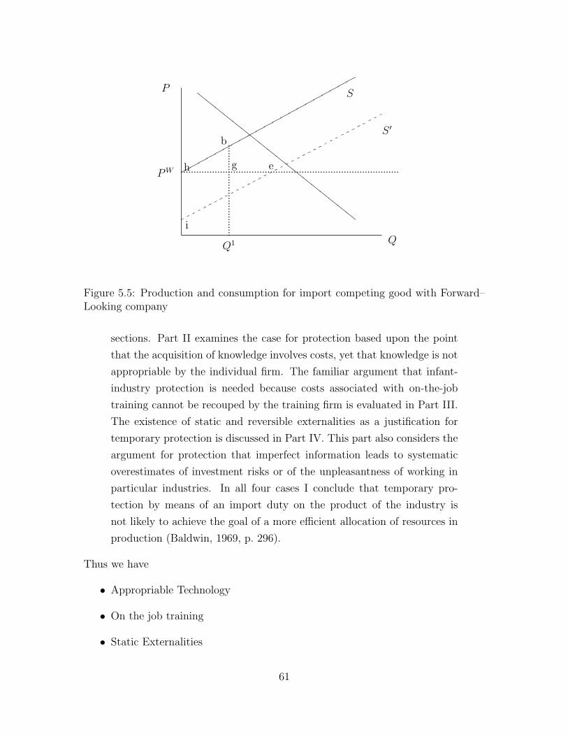
���������������������
cc
cc
cc
cc
cc
cc
cc
cc
cc
Q
P
PW
S
S ′
...................................................................................eh
i
...................................Q1
b
g
Figure 5.5: Production and consumption for import competing good with Forward–Looking company
sections. Part II examines the case for protection based upon the point
that the acquisition of knowledge involves costs, yet that knowledge is not
appropriable by the individual firm. The familiar argument that infant-
industry protection is needed because costs associated with on-the-job
training cannot be recouped by the training firm is evaluated in Part III.
The existence of static and reversible externalities as a justification for
temporary protection is discussed in Part IV. This part also considers the
argument for protection that imperfect information leads to systematic
overestimates of investment risks or of the unpleasantness of working in
particular industries. In all four cases I conclude that temporary pro-
tection by means of an import duty on the product of the industry is
not likely to achieve the goal of a more efficient allocation of resources in
production (Baldwin, 1969, p. 296).
Thus we have
• Appropriable Technology
• On the job training
• Static Externalities
61

• Imperfect Information about risks and benefits
5.4.1 Appropriable Technology
Industrialization is here at first wholly a matter of imitation and impor-
tation of tried and tested processes (Hirschman, 1968, p. 7).
Here industrialization is a process of imitation not creation. New technologies are
not being created, old ones are being followed. In many of the industries, intermediate
goods are imported at the early stage. Note that this suggests that the Heckscher–
Ohlin model is a good way to describe economies in this stage at least in a static
sense.
5.4.1.1 Example of Spillovers from Investment in Technology
[This example is attributed to J. McLaren’s lecture notes] Consider an economy with
a large number of identical farmers. Each farmer enjoys leisure and food, and must
divide her time between leisure time and work on her farm. For simplicity, we will
assume that all of the time each farmer spends working is devoted to researching
new techniques. (All of the routine business of planting, hoeing, and so forth could
be added and would simply add complication without changing the point.) The
production possibilities of a particular farmer, holding the actions of all other farmers
constant, are indicated by the heavy curve in Figure 5.6. We will call this the “private
production possibility frontier.” The more time the farmer spends on research and
experimentation, the more effective the farm will be and thus the more output she
will receive. The farmer’s preferences are indicated by the lighter, convex curve in
Figure 5.6. She chooses the level of research effort that maximizes her utility, given
the environment, and that optimum is given by point A.
The private PPF shows how much additional output a particular farmer would
receive if she alone worked an extra hour. However, suppose that some portion of the
knowledge generated by a farmer as part of that farmer’s research effort can be used
by other farmers who observe or hear about that farmer’s discovery and apply it to
their own farms. Call this the “spillover” assumption. In that case, if every farmer
worked an extra hour, the additional output any one farmer would receive would be
greater than the additional output that farmer would have received if she alone was
putting in the extra hour, because aside from benefiting directly from her own efforts
she would benefit indirectly from the ideas of others. This is represented by the light
62

time
output
leisure research time- �
A
Figure 5.6: Private PPF for farmer engaged in research
concave curve in Figure 5.7, which plots the output each farmer would receive for any
given level of research effort, if that level of effort was put in by all farmers together.
Thus, as we move along the light concave curve, we vary the work effort of every
single farmer in the economy by the same amount. We call this curve the “social
production possibility frontier” and note that because of the spillover assumption it
is strictly steeper than the private PPF.1
Because the social PPF is steeper than the private PPF, we see immediately that
all farmers would be made better off if all of them together could be induced to work
a little bit harder; this would allow each farmer to move from A to B in Figure 5.7,
which is on a higher indifference curve and therefore preferred. This could be brought
about, for example, by a subsidy to research effort, financed by a lump sum tax, so
that each farmer would have to give up x bags of grain to the government, but could
then get y bags of grain back per unit of output. If things were designed just right,
in equilibrium each farmer would get back exactly the amount of the lump-sum tax
and the only effect would be to encourage additional research effort, thus moving the
economy from A to B. On the other hand, Figure 5.8 shows that point B cannot
be brought about without government intervention or some similar mechanism, and
1We have designed the social PPF so that it intersects with the private PPF at point A fromFigure 5.6. This is deliberate, so that the analysis is interesting, but we could have drawn a seriesof social PPF curves with different intersections.
63
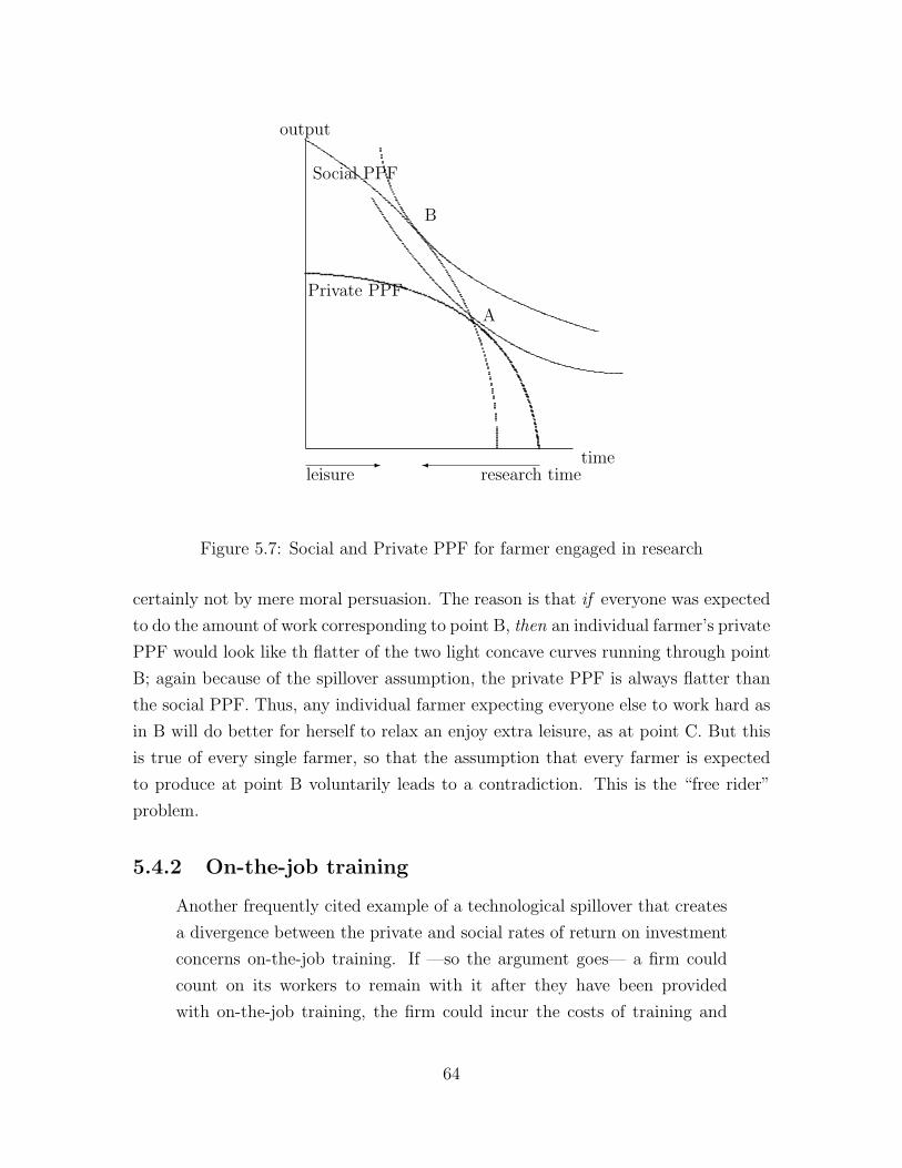
time
output
leisure research time- �
A
Private PPF
Social PPF
B
Figure 5.7: Social and Private PPF for farmer engaged in research
certainly not by mere moral persuasion. The reason is that if everyone was expected
to do the amount of work corresponding to point B, then an individual farmer’s private
PPF would look like th flatter of the two light concave curves running through point
B; again because of the spillover assumption, the private PPF is always flatter than
the social PPF. Thus, any individual farmer expecting everyone else to work hard as
in B will do better for herself to relax an enjoy extra leisure, as at point C. But this
is true of every single farmer, so that the assumption that every farmer is expected
to produce at point B voluntarily leads to a contradiction. This is the “free rider”
problem.
5.4.2 On-the-job training
Another frequently cited example of a technological spillover that creates
a divergence between the private and social rates of return on investment
concerns on-the-job training. If —so the argument goes— a firm could
count on its workers to remain with it after they have been provided
with on-the-job training, the firm could incur the costs of training and
64
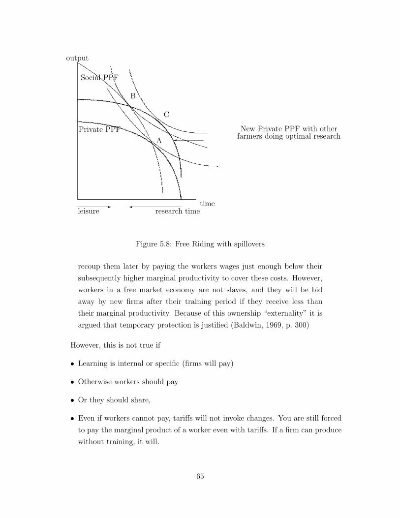
time
output
leisure research time- �
A
Private PPF
Social PPF
B
New Private PPF with otherfarmers doing optimal research�
C
Figure 5.8: Free Riding with spillovers
recoup them later by paying the workers wages just enough below their
subsequently higher marginal productivity to cover these costs. However,
workers in a free market economy are not slaves, and they will be bid
away by new firms after their training period if they receive less than
their marginal productivity. Because of this ownership “externality” it is
argued that temporary protection is justified (Baldwin, 1969, p. 300)
However, this is not true if
• Learning is internal or specific (firms will pay)
• Otherwise workers should pay
• Or they should share,
• Even if workers cannot pay, tariffs will not invoke changes. You are still forced
to pay the marginal product of a worker even with tariffs. If a firm can produce
without training, it will.
65

5.4.3 Static Externalities
Static externalities do not require temporary tariffs as a solution, but rather perma-
nent subsidies. Honey and Apples example.
5.4.4 Imperfect Information
If it is hard to know whether or not an industry is competitive it is hard to imagine
that producing in a tariff protected environment will really answer that question. If
you can see that it is profitable with tariffs, but cannot see that it is profitable without
them, how will producing with tariffs teach you that it is profitable?
5.5 Backward Linkages
The tuner example. Basic idea is that there is nothing obvious about backwards
linkages being created and that the forwards industry might loose considerably if the
backward industry gets protected.
5.6 Latin American Experience
Three principal accusations have been leveled against the industrialization
process as it has appeared in Latin America:
1. Import Substituting Industrialization is apt to get “stuck” after its
first successes, due to the “exhaustion of easy import substitution
opportunities”; it leave the economy with a few relatively high-cost
industrial establishments an with a far more vulnerable balance of
payments since import consist now of semifinished materials, spare
parts and machinery indispensable required for maintaining and in-
creasing production and employment.
2. import substituting industry is affected by seemingly congenital abil-
ity to move into export markets.
3. The new industries are making an inadequate contribution to the
solution of the unemployment problem.
Hirschman (1968, p. 13)
66

Chapter 6
Monopolistic Competition and
World Trade Patterns
6.1 Introduction
We have been considering the case, so far, of choosing between free trade and no
trade. In the case of Import Substituting Industrialization the choice was a bit more
complex; that of choosing between free trade and protection for a given good. In
fact the choices on trade are often more complex than this. The United States is an
excellent example of the degrees of free trade or protectionism that can be exhibited.
The U.S. is a champion of General Agreement on Tariffs and Trade (GATT) and now
the World Trade Organization (WTO). We push free trade throughout the world.
Yet some of our industries have been, and remain, highly protected from foreign
competition. And at the same time we are engaged in a very significant free trade
area with Canada and Mexico, NAFTA, and are in talks with other nations about
the possible expansion of the Free Trade Area of the Americas (FTAA).
Whenever the U.S. restricts imports from foreign countries it hurts domestic con-
sumers of those goods by raising the price they have to pay for them. Although it
benefits domestic producers, we know that there are net efficiency losses for the wel-
fare of the United States. When the trade barriers are in the form of quotas then it
is very likely that there are large transfers of quota rents to overseas producers of the
goods in question. These transfers can be thought of as net loses, or the U.S. could
consider these transfers as a form of foreign aid. When the quota is on the importa-
tion of Japanese automobiles, it is very hard to see that domestic policy makers might
67

want to transfer funds from U.S. consumers to Japanese automobile producers; this
policy is most likely an underhanded way to transfer funds to domestic automobile
producers.
However when we examine trade regimes such as the Multi-Fiber Arrangement
(MFA) we see that the U.S. might deliberately be handing rents to foreign countries
as a type of aid. It helps domestic textile manufacturers, but it also helps foreign
importers. To help in our analysis of the impact of these patterns we look at the
model of monopolistic competition
6.2 Monopolistic Competition
We know that a monopolist does not take the price at which he sells goods as given,
but rather that a monopolist understands the impact that his quantity decisions can
have on the price. The monopolist seeks to maximize profits and this leads him to
set the marginal cost equal to the marginal revenue.
In the setting of monopolistic competition this is also true. However the demand
curve faced by the monopolist will be a function of the decisions made by other players
in the market. None the less if there are enough players in the market (we are not
in a duopoly or oligopoly situation) the player will take his demand curve as given
and seek to maximize profits. If there are profits in the industry then this can attract
other entrants (since they believe they could also make profits). An increase in the
supply of the good will lead to a change in the demand curve faced by every remaining
player in the market. Equilibrium will be achieved when every player is maximizing
its profits but profits are equal to zero (or profits for the next entrant would be either
zero or negative). This situation is represented in Figure 6.1.
We will assume that each firm faces a demand function as shown in Equation 6.1.
q = Q ·(
1
n− b (p− p̄)
)(6.1)
We assume a simple cost structure for the firm as shown in Equation 6.2
C = F + c · q (6.2)
68

Q
P@
@@
@@
@@
@@
@@
@@
@@
AAAAAAAAAAAAAAAAAAAA
MC
AC
Q?
P ?
Demand
Marginal Revenue
Figure 6.1: Profits driven to zero in Monopolistic Competition
variable definition
q firm quantity
Q Industry Quantity
n number of firms
b responsiveness of sales to firm price
p firm price
p̄ industry average price
c marginal cost
F Fixed cost
Thus the average cost is Fq
+ c and is declining in quantity produced. There are
economies of scale in production.
We want to know what the number of firms will be in a monopolistically compet-
itive industry. We use the above model and assume that there is an infinite supply
of identical firms that could enter the industry. How many would enter? On the one
hand as more and more firms enter the industry the average cost for the remaining
firms will go up, suggesting that if the price of the good is high, more firms will enter.
On the other hand, as more and more firms enter the industry the price earned by
the firms in the industry must fall since they face more and more competition. If
we think of the first effect as a type of supply of firms (increasing in price) and the
second as a type of demand for firms (decreasing in price) we can find the equilibrium
69
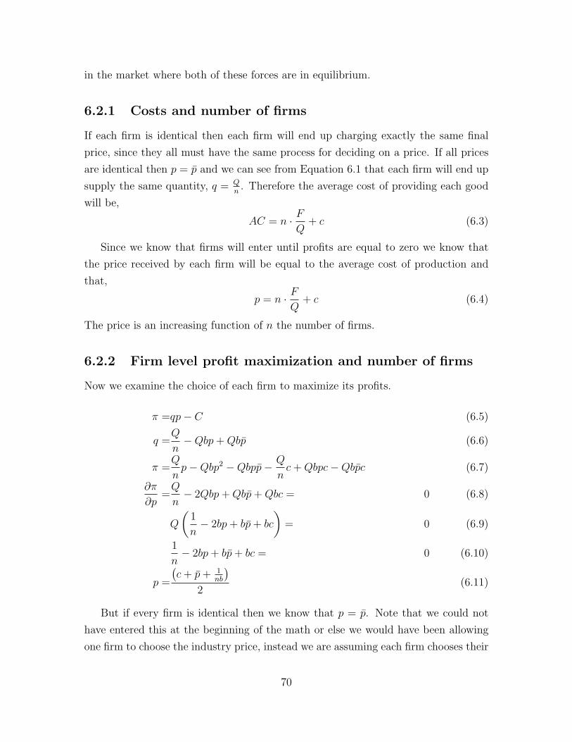
in the market where both of these forces are in equilibrium.
6.2.1 Costs and number of firms
If each firm is identical then each firm will end up charging exactly the same final
price, since they all must have the same process for deciding on a price. If all prices
are identical then p = p̄ and we can see from Equation 6.1 that each firm will end up
supply the same quantity, q = Qn. Therefore the average cost of providing each good
will be,
AC = n · F
Q+ c (6.3)
Since we know that firms will enter until profits are equal to zero we know that
the price received by each firm will be equal to the average cost of production and
that,
p = n · F
Q+ c (6.4)
The price is an increasing function of n the number of firms.
6.2.2 Firm level profit maximization and number of firms
Now we examine the choice of each firm to maximize its profits.
π =qp− C (6.5)
q =Q
n−Qbp + Qbp̄ (6.6)
π =Q
np−Qbp2 −Qbpp̄− Q
nc + Qbpc−Qbp̄c (6.7)
∂π
∂p=
Q
n− 2Qbp + Qbp̄ + Qbc = 0 (6.8)
Q
(1
n− 2bp + bp̄ + bc
)= 0 (6.9)
1
n− 2bp + bp̄ + bc = 0 (6.10)
p =
(c + p̄ + 1
nb
)2
(6.11)
But if every firm is identical then we know that p = p̄. Note that we could not
have entered this at the beginning of the math or else we would have been allowing
one firm to choose the industry price, instead we are assuming each firm chooses their
70

own price (holding industry price fixed), but this turns out to be the industry price.
Thus Equation 6.11 becomes Equation 6.12.
p = c +1
nb(6.12)
Thus the price charged by each firm is a decreasing function of the number of other
firms and the responsiveness of that firms quantity to its price, but an increasing
function of its marginal cost. This makes sense. The more other firms there are, and
the closer the products they make are to the product that you sell, the lower your
price. Note that price cannot be lower than the marginal cost because both b and n
are positive.
6.2.3 Equilibrium
We now have two equations (Equation 6.4 and Equation 6.12) in two unknowns (p
and n) and we can solve for both.
p = c +1
nb=n
F
Q+ c (6.13)
1
nb=n
F
Q(6.14)
n =
√Q
Fb(6.15)
p =
√F
Qb+ c (6.16)
q =√
QbF (6.17)
Thus we can see that the number of firms is increasing in the total demand and
decreasing in the fixed cost and substitutability of goods. The price is equal to the
marginal cost plus a function which in increasing in fixed costs, decreasing in quantity
and substitutability.
6.2.4 Numerical Example of Monopolistic Competition
Assume two countries that each produce automobiles but do not trade at first. The
cost of automobile production in each country (and for each producer in each country)
is the same but the initial demand is not the same:
71

variable value
F 750,000,000
c 5,000
b 130,000
QA 900,000
QB 1,600,000
We can do the math and we get the following values
variable value
nA 6
nB 8
pA 10,000
pB 8,750
QA 150,000
QB 200,000Now we allow the two countries to trade with each other and thereby allow each
country to face a total market demand of 2.5 million cars. Now we end up with 10
firms each selling 250,000 cars at a price of $8,000. Note that there is no comparative
advantage and no relative abundance, and yet we will end up with trade between
these two countries that is beneficial to consumers. The total number of producers
has fallen from 8 + 6 = 14 to 10, but the price has fallen, and since there were no
profits in either case, producers cannot have lost. Each firm has a larger supply.
72

Bibliography
Baldwin, R. E., “The Case Against Infant-Industry Protection,” The Journal ofPolitical Economy, 1969, 77, 295–305.
Harrison, A., “An empirical test of the Infant Industry Argument: Comment,”American Economic Review, 1994, 84 (4), 1090–5.
Hirschman, A., “The Political Economy of Import–Substituting Industrialization,”Quarterly Journal of Economics, 1968, 82 (1).
Krueger, A. O., “The Political Economy of the Rent Seeking Society,” AmericanEconomic Review, 1974, 64, 291–303.
and B. Tuncer, “An empirical test of the Infant Industry Argument,” AmericanEconomic Review, 1982, 72 (5), 1142–52.
Magee, S. P., “Three Simple Tests of the Stolper-Samuelson Theorem,” in “BlackHole Tariffs and Endogenous Policy Theory,” New York: Cambridge UniversityPress, 1989, chapter 7.
Wood, Adrian, “Openess and Wage Inequality in Developing Countries: The LatinAmerican Challange to East Asian Conventional Wisdom,” World Bank EconomicReview, 1997, 11 (1), 33–57.
73

Index
absolute advantage, see advantage, ab-solute
advantage, absolute, 9, 19advantage, comparative, 9, 19assumption
perfect competition, 35small country, 14, 34
average product of labor, 25
budget constraint, 11
capital-labor ratio, 40comparative advantage, see advantage,
comparativeconcave, 13, 63constant returns to scale, 40convex, 13, 39, 62CRS, see constant returns to scale
diminishing marginal productivity, 21diminishing marginal returns, 21diminishing returns, 13, 21duopoly, 68
example, 62
factor intensity, 32, 33Factor Proportions Model, 31–53fixed coefficients, 31, 31–39
GATT, see General Agreement on Tradeand Tariffs
General Agreement on Trade and Tar-iffs, 67
Heckscher–Ohlin Model, 31–53, 62
Import Substituting Industrialization,56–66
import substituting industrialization, 56,58, 60, 66, 67
indirect production possibility frontier,see production possibility fron-tier, trade augmented
infant industry protection, see importsubstituting industrialization
ISI, see import substituting industrial-ization
isocost frontier, 40isoquant, 39–42
unit, 40
k, see capital-labor ratio
labor allocation frontier, 21, 22labor, marginal product of, see marginal
physical product of laborLerner diagram, 41luxury good, 15
marginal physical product, 22–25, 28,43
of labor, 22–25, 28marginal product of labor, see marginal
physical product of labormarginal rate of technical substitution,
39, 40diminishing, 39
marginal value product, 29marginal value product of labor, 22Monopolistic Competition, 67–72monopolistic competition, 68MPL, see marginal physical product of
laborMRTS, see margainal rate of technical
sustitution
74
offer curve, 14oligopoly, 68
political economy of trade, 20PPF, see production possibility frontierPrebisch-Singer, 56prices
Factor–Proportions, 34Heckscher–Ohlin, 34
production possibility frontier, 10–14,17, 18, 20, 22, 23, 32–34, 47,48, 62–64, 74, 75
biased expansion of, 47trade augmented, 11, 14
rate of techinical substitution, see mar-gainal rate of technical sustitu-tion
Ricardian Model, 19, 7–19, 20, 33, 34,52
Ricardo–Viner–Cairnes, 52RTS, see margainal rate of technical
sustitutionRybczynski Theorem, 46, 47
Specific Factors Model, 20–30, 42, 52spillover, 62Stolper–Samuelson, 45Stolper–Samuelson Theorem, 36strong factor intensity, 40
terms of trade, 56trade augmented production possibility
frontier, see production possi-bility frontier, trade augmented
variable coefficients, 39–53
wages, 19nominal, 24real, 24ricardian, 19
World Trade Organization, 67WTO, see World Trade Organization
75

Glossary
C
concave A set is said to be convex if the line joining any two points of the set liesentirely within the set. A function is concave on a the convex set D if theset defined by x, x ∈ D and all points less than f(x) form a convex set. Afunction is convex on the convex set D if the set defined by x, x ∈ D andall points greater than f(x) form a convex set. In simpler language, ona two dimensional graph, all the points on and below a concave functionform a convex set, and all the points on and above a convex function forma convex set.
convex See the definition of concave.
G
General Agreement on Tariffs and Trade (GATT) The General Agreement on Tar-iffs and Trade was established in 1947 and is headquartered in Geneva. TheUruguay Round is the most recent change in GATT. It is the eight roundof negotiations and it begain in Punta del Esta, Uruguay in 1986 and wascompleted with a signing in Marrakesh, Morrocco in 1994. The secre-tariat of GATT was replaced by the World Trade Organization (WTO) asa result of the Uruguay Round treaties.
I
Import Substituting Industrialization (ISI) A deliberate government policy shield-ing “infant” industries from international competition, usually accom-plished through high import tarrifs or other trade bariers.
isoquant The locus of alternative combinations of productive inputs that can beused to produce a given level of output.
M
marginal rate of technical substitution (MRTS) The rate at which one input maybe traded off against another in the productive process while holding out-
76

put constant. The RTS is the absolute value of the slope of the isoquant.
P
production possibility frontier (PPF) The locus of all the alternative quantities ofseveral outpus that can be produced with fixed amounts of productiveinputs.
T
terms of trade The price of a countries exports divided by the price of its imports.PX
PM.
trade–augmented production possibility frontier (trade–augmented PPF) The lo-cus of all the alternative quantities of several outpus that can be consumedgiven domestic production and world prices.
W
World Trade Organization (WTO) The World Trade Organization is a new nameapplied to the secretariat of the General Agreement on Trade and Tariffs.
77


![[Economic Policy Making] Fiscal Policy](https://img.pdfslide.us/doc/110x75/5a4d1bf67f8b9ab0599e8d15/economic-policy-making-fiscal-policy.jpg)