MICROECONOMICS at UNYP Dan Stastny

Page 1 Printed: 4/13/2012 at 8:52 AM

Warning: This study guide is provided “as-is”; there is no responsibility of the author for any errors or omissions!

MICROECONOMICS at UNYP

Dan Stastny Outline by Chapters: 1. Introduction to Economics 2. Consumer Theory 3. Producer Theory I 4. Market 5. Producer Theory II 6. Market Structure 7. Input Markets


Chapter 1 Introduction to Economics

Outline: 1.1 What is Economics and what is it for? 1.2 Methodology of Economics 1.3 Logic of Choice 1.4 Dealing with Scarcity 1.1 What is Economics and what is it for?

- science about human action (decision-making) and its consequences 1.2 Methodology of Economics

I. M. DUALISM - natural vs. social sciences

II. M. INDIVIDUALISM - keep an eye on the individual

III. FULL EFFECTS - make sure to include everything, not just the seen, but also the unseen

1.3 Logic of Choice - WHY choosing/acting/decision-making?

- SCARCITY = THE economic problem - HOW people act (make choices)

i. UTILITY - ordinal magnitude of “pleasure”, “satisfaction” ii. COST - utility of the best alternative foregone (given up)

- importance of only MARGINAL units:

- marginal utility and marginal cost - common errors: sunk cost and average cost

The economic way of thinking

MU > MC 1.4 Dealing with Scarcity - EVERY ACTION AIMED AT REDUCING SCARCITY

- goods must be produced => importance of productivity - outward movement of PPF


- METHODS OF INCREASING THE PRODUCTIVITY (i.e. alleviating scarcity) i. Physical capital ii. Human capital iii. Cooperation division of labor exchange - alternative to different technology

- LAW OF COMPARATIVE COST

- determination of specialization and exchange pattern


Chapter 2 Consumer Theory

Outline: 2.1 What is it for? 2.2 The model: “Robinson & Friday” Economy 2.3 Law of Demand and the Demand Curve 2.4 Factors Influencing Quantity Demanded 2.5 Price Elasticity of Demand 2.1 What is it for? 2.2 The Model: “Robinson & Friday” Economy - two people (R&F), two goods (fish and squirrel) economy

Squirrel

Robinson Friday

Fish

- - - questions:

- how many squirrels he will be interested to get? - how much fish will he be willing to pay?

- thought experiment

squirrel 1st 2nd 3rd 4th 5th 7th ...

# of fish 10 9 8 7 6 5

⇒ Law of Diminishing Marginal Utility - every additional unit of a good is valued less than the previous unit

# fish

per one squirrel

# fish per one squirrel

# squirrel # squirrel

2.3 Law of Demand and the Demand Curve ⇒ Demand Curve - relationship between the price and quantity demanded ⇒ Law of Demand

D [MU] MU


- the higher the price, the lower the quantity demanded and vice versa

P

Q - demand curve falling because of:

a) Law of Diminishing Marginal Utility b) Substitution Effect c) Income Effect

2.4 Factors Influencing the Quantity Demanded QD Price (P)

Preference for this good relative to other goods

Expectations Income normal inferior Prices of other goods substitutes complements

2.5 Price Elasticity of Demand

|ePD| > 1 elastic |ePD| = 1 unitarily elastic |ePD| < 1 inelastic

- determinants of price elasticity

- urgency of need the good satisfies - the more urgent, the less elastic

- length of time under consideration - the longer period, the less elastic

- variety of substitutes - the more substitutes, the more elastic

- share of the outlays on the good relative to total spending - the smaller the share, the less elastic

******************** Concept of demand curve (and law of demand) is a universal one

ePD = % ∆ QD

% ∆ P

D [determined by MU]

“shifting” the curve

“moving along” the curve


Chapter 3 Producer Theory I.

Outline: 3.1 What is it for? 3.2 The model: “Robinson & Friday” Economy 3.3 Law of Supply and the Supply Curve 3.4 Factors Influencing Quantity Supplied 3.5 Price Elasticity of Supply 3.1 What is it for? 3.2 The Model: “Robinson & Friday” Economy - two people (R&F), two goods (fish and squirrel) economy

Squirrel

Robinson Friday

Fish

- questions: - how many squirrels will Friday be willing to give up? - how much fish will will he require in return?

- thought experiment

squirrels to be given up 1st 2nd 3rd 4th 5th 7th ...

# of fish (minimum) 2 3 4 5 6 7 ...

# fish

per one squirrel

# fish per one squirrel

# squirrel # squirrel 3.3 Law of Supply and the Supply Curve ⇒ Supply Curve - relationship between the price and quantity supplied ⇒ Law of Supply, or Law of Increasing Marginal Cost - the higher the price, the higher the quantity supplied and vice versa

S [MC] MU given up

= MC


P

Q - supply curve upward-sloping because of: a) Law of Diminishing Marginal Utility b) Law of Diminishing Marginal Productivity (or Law of Diminishing Returns to

Variable Factor) - in the real world, the act of supply presupposes an act of production

Inpu

ts:

labo

r, la

nd a

nd

capi

tal g

oods

I1 Production

Outputs:

consumer or

capital goods

I2 O1

I3 O... I4 I...

⇒ how much resources it takes to produce marginal units of the good?

- the same as asking how many units of output will an additional unit of input produce

⇒ marginal productivity

# of hours ... 5 6 7 8 9 ... Total product (TP, # of squirrels)

... 20 25 29 32 33 ...

Marginal product (MP, # of squirrels)

... - 5 4 3 1 ...

- the law reads: if only one factor of production is variable, then there is

always a certain quantity of that input beyond which each additional unit contributes less to total product then the previous unit

S [determined by MC]


3.4 Factors Influencing the Quantity Supplied

QS Price (P)

Seller’s preference for this good relative to other goods

Expectations Productivity of inputs Prices of inputs (factors of production) Prices of output (production)

substitutes

3.5 Price Elasticity of Supply

ePS > 1 elastic ePS = 1 unitarily elastic ePS < 1 inelastic

- determinants of price elasticity

- length of time under consideration (the longer period, the more elastic) - input-specificity of output (the more specific inputs, the less elastic)

******************** Concept of supply curve (and law of supply) is a universal one

ePS = % ∆ QS

% ∆ P




S [determined by MC of all sellers]

D [determined by MU of all buyers]

(QD=QS)

P*

Q*

DMARKET

DPETER

5 DPAUL

5 5

9 2 3 5 5 4

3.50 3.50 3.50

Chapter 4 Market and Equilibrium

Outline: 4.1 What is Market and Equilibrium? 4.2 Changes in Equilibrium 4.3 Market and Efficiency 4.4 Interference in the Market 4.5 Market Failures 4.1 What is Market and Equilibrium? - market

- “an array of all voluntary exchanges” - how to get market demand and supply from individual demand and supply?

- horizontal sum (summing quantities across the price)

P P P

Q Q Q

- drawing both D and S into one graph will yield the “big picture”:

P

Q - market equilibrium

- a situation in which no one in the market is motivated to change his decision - equilibrium price and quantity: P* and Q* - QS = QD

- real-world equilibrium: never actually reached due to permanent changes of conditions - ceteris paribus = other things being equal

3


D0

P0

Q0

D1

Q1

P1

QS < QD



P*

Q*

Consumer Surplus

Producer Surplus

S

Q1

D0

P0

Q0

D1

P1

Q1

D0

Q0

D1

P0

P1

S

4.2 Changes in equilibrium - influence of changes in any condition enters through change in either D or S - coordinating function of the price

P

Q

- influence of elasticities upon the magnitude of change

P P

Q Q 4.3 Market and Efficiency - efficiency

- situation is efficient if no one in the society can be made better off without making anybody else worse off (so called Pareto efficiency)

- market outcomes are efficient:

P

Q

S


Loss of efficiency

S [MC]

Surplus

QD < QS

PMIN

PMIN – additional cost

Free market P

D [MU]

Total additional cost born by sellers

D [MU]

S [MC]

Shortage

QS < QD

PMAX

PMAX + additional cost

Free market P

Total additional cost born by buyers

Loss of efficiency

4.4 Interference in the Market a) price controls

Price Ceiling

P

Q

Price Floor

P

Q - price prevented from adjusting the QS and QD

- alternative means of adjustment: - bribes, extra payments - lines (“first come, first serve”)

- competition means additional cost to paying (or receiving) the price - this cost is either someone else’s benefit (e.g. bribes) or it is net waste (e.g.

standing in the line) - loss of efficiency (a “dead-weight loss” – DWL)

- lost consumer/producer surplus that is no one else’s benefit - only under black market there is (almost) no DWL!


D [MU]

S [MC]

QAFTER-TAX QPRE-TAX

PPRODUCER

PPRODUCER + Tax = PCONSUMER

PPRE-TAX

Total Tax Revenue for the Government

Loss of efficiency

S [MC + incl. the Tax]

PPRODUCER

D [MU]

D [MC + subsidy]

QPRE-SUB QAFTER-SUB

PPRODUCER – Subsidy = PCONSUMER

PPRE-SUB

Total amount of Subsidy paid out by the government

Loss of efficiency

S [MC]

b) Taxes and subsidies

Imposed on

Buyer (Consumer)

Seller (Producer)

Type

of

Inte

rven

tion Tax D shifts

Left S shifts

Left

Subs

idy

D shifts Right

S shifts Right

Tax Imposed on Supplier

P

Q

Subsidy Provided to Buyer

P

Q




P*

Q*

Loss of Efficiency

People who get their transplants

PMAX = 0

People who won’t…

c) Bans and Regulations - ban on trading

- e.g. human organs

P

Q

- - product regulations

4.5 Market Failures

a) Imperfect information (information asymmetry) - real MU or MC are different from those perceived by decision-making

individuals

b) Spill-over Effects i. Externalities - existence of external MU or MC => real MU or MC are different from those

that decision-making individuals take into account ii. Public Goods - so large an externality, so that the good might not be produced at all, even

though people value it more than the cost of production

c) Market Power - power of buyer or seller to influence market price (i.e. “monopoly”)

- does NOT mean that it can be improved by intervention!!!


Chapter 5 Producer Theory II.

Outline: 5.1 Profit Maximization Assumption 5.2 Decisions of How Much to Produce 5.3 Decisions of How to Produce: Efficiency in Production 5.4 Theory of the Firm (or Why Are Firms?) 5.1 Profit Maximization Assumption - special term for utility of producers: profit

Total (Economic) Profit (π) = Total Revenue (TR) – Total Cost (TC)

Tota

l Cos

t: C

ost o

f usi

ng a

ll in

puts

I1 Production Total Revenue:

Revenue from

producing (and

selling) all outputs

I2 O1

I3 O... I4 I...

- Total Revenue (or Cost) includes not only explicit items, but also implicit ones

- Implicit Revenue: psychic utility, non-monetary benefits

- Implicit Cost: opportunity cost of using one’s own resources, i.e. resources for which one does not get charged anything explicitly

Total Revenue – Total Cost

Total Profit = Explicit Revenue – Explicit

Cost + Implicit Revenue – Implicit

Cost Accounting Profit


- normal profit: a profit when economic profit equals zero

Items per Year Revenue Cost Sales 1,500,000 Purchase of Supplies 150,000 Heating 20,000 Wages 120,000 Explicit Revenue and Cost 1,500,000 290,000

Accounting Profit 1,210,000 Implicit Wage 210,000 Implicit Rent 1,000,000

Total (Economic) Profit 0

- generally, profits in all industries tend to be normal - businesses move from industries with lower profits to industries with higher

profits: tendency to profit equalization across industries - importance of profit maximization

- reward for not wasting (see further below) - proof of usefulness in social cooperation

5.2 Decisions of How Much to Produce - profit maximization assumption is a particular form of the general prescription for

economic behavior: MU > MC - utility is here called revenue: MU is turned into MR

- it pays to produce more as long as MR > MC, until

MR = MC

“golden rule” of profit maximization - recap:

- marginal revenue: additional revenue associated with selling one more unit of output

- marginal cost: additional cost associated with producing one more unit of output


Profit Maximization Rule

P and MC

[in $]

Q - the “golden rule” is “slippery”: it is only necessary, but not sufficient for profit-

maximization - it is also necessary to find out whether it pays to produce the particular quantity

suggested by the golden rule (i.e. Q*) - when will it “pay”?

- answer dependent on the time horizon: whether it is a short- or a long run

a) Short Run - period in which only one factor of production is variable (i.e. adjustable) - total cost to the producer can then be distinguished as follows:

- variable cost (VC): cost of using variable inputs - fixed cost (FC): cost of using fixed inputs (must be born regardless of the

quantity produced) ⇒ TC = FC + VC

- fixed cost, in the short run, are sunk cost: cost irrelevant for the decision of

whether and how much to produce ⇒ in the short run, it pays to produce as long as TR ≥ VC • otherwise (i.e. only if TR < VC), it pays to stop producing, i.e. to “shut

down”

- to certain extent, in the short run, it might pay to be producing despite running overall economic (or even accounting) losses! - why? because losses are then smaller than if the business stopped

producing altogether (losses are minimized)

b) Long Run - period in which all factors are variable (i.e. adjustable) - no fixed cost means that all costs are relevant (none are sunk) ⇒ in the long run, it pays to produce as long as TR ≥ TC • otherwise (i.e. if TR < TC), it pays to stop producing, i.e. to “shut down”

- in the long run, producers shut down their businesses if they have lower than

normal profit

Q*

P0

MC

MR


5.3 Decisions of How to Produce: Efficiency in Production - profit motivation encourages producers to behave efficiently, i.e. not to waste - what is economically efficient production?

- situation when a given quantity of output cannot be produced at lower cost - different from technical efficiency of production, which only requires that with

given inputs maximum possible amount of output is produced ⇒ drive for lowest possible cost determines the proportions of inputs used in

production a) Short Run - proportions among fixed factors is (well, guess…)…. fixed - adjusting only one variable factor: efficiency in production requires that given

quantity is produced with the least possible amount of variable input - average cost of production (TC/Q) is sooner or later increasing (which is due to the

law of diminishing returns) b) Long Run - more complicated as all factors of production are variable - efficiency in production (i.e. the least-cost criterion) requires that an additional

dollar’s worth of any input must produce the same additional output:

- marginal product (MP) of each input (A, B, C, …, n) must be proportional to its price (P)

MPA = MPB = MPC = MPn

PA PB PC Pn

equimarginal principle

- in the long run, average cost of production depends on whether there are economies

of scale (EOS) or diseconomies of scale (DOS) - if you want to produce k-times more, it also cost you more, say, x-times

- if x < k, the production exhibits EOS and average cost is decreasing - if x > k, the production exhibits DOS and average cost is increasing

5.4 Theory of the Firm (or Why Are Firms?) - institutionally, production takes place largely within firms

- why is it so if all production could be decentralized and take place without any single firm?

- much of the cooperation among people takes place outside of the firm: on the market

- the answer: dealing on the market has its cost


- finding and securing required factors of production - cost of contracts and their renewing

⇒ it might pay to make long-term and universal contracts: to establish a firm - saves cost also by deepening specialization:

- people who have hard times organizing themselves and do not like to bear the uncertainty associated with running the business become salaried workers

- people who stand out in their managing or entrepreneurial capabilities become managers or outright employers

- however, replacing market with bureaucracy (hierarchy) within firms has also its

cost - supervision - bureaucratic organization

⇒ this is rising exponentially with the size of the firm - real-world size and structure of firms depends on the above two considerations:

- different in each industry, reflecting differences in the point at which the costs associated with the operation of a firm begin to outweigh the economies gained from establishing the firm

- this is also reflected in the type of the firm

- individual entrepreneurs vs. partnerships, limited companies or corporations


Chapter 6 Market Structure

Outline: 6.1 Perfect and Imperfect Competition 6.2 Monopoly 6.3 Oligopoly 6.4 Monopolistic Competition 6.5 Real-world Competition 6.1 Perfect and Imperfect Competition - key concept: market power

- capability of particular market participant to influence market prices Perfect Competition - no market participant has any market power: all are price-takers

- individual producers face perfectly elastic demand for their products - individual buyers face perfectly elastic supply of the products they buy

- in this market MU=P=MC ⇒ efficiency - perfect competition is said to exist under following conditions:

- infinite numbers of buyers and sellers - perfect and free information - homogeneous product - no barriers to entry

- conceptually impossible model world, misused as ethical benchmark Imperfect Competition - some participants DO have market power: some are price-searchers (price-makers)

- individual producers face downward sloping demand: monopoly power - individual buyers face upward sloping supply: monopsony power

- monopoly power - decision about the combination of P and Q (given by the demand) - how? MR=MC

- MR downward sloping (and faster than demand itself) due to monopoly power

Profit Maximization under Monopoly Power

P and

MC [in $]

Q Q*

P0

MR

MC

dF


- P>MC: inefficiency ⇒ “market failure”

- yes, but… - in real world all producers have some market (monopoly) power

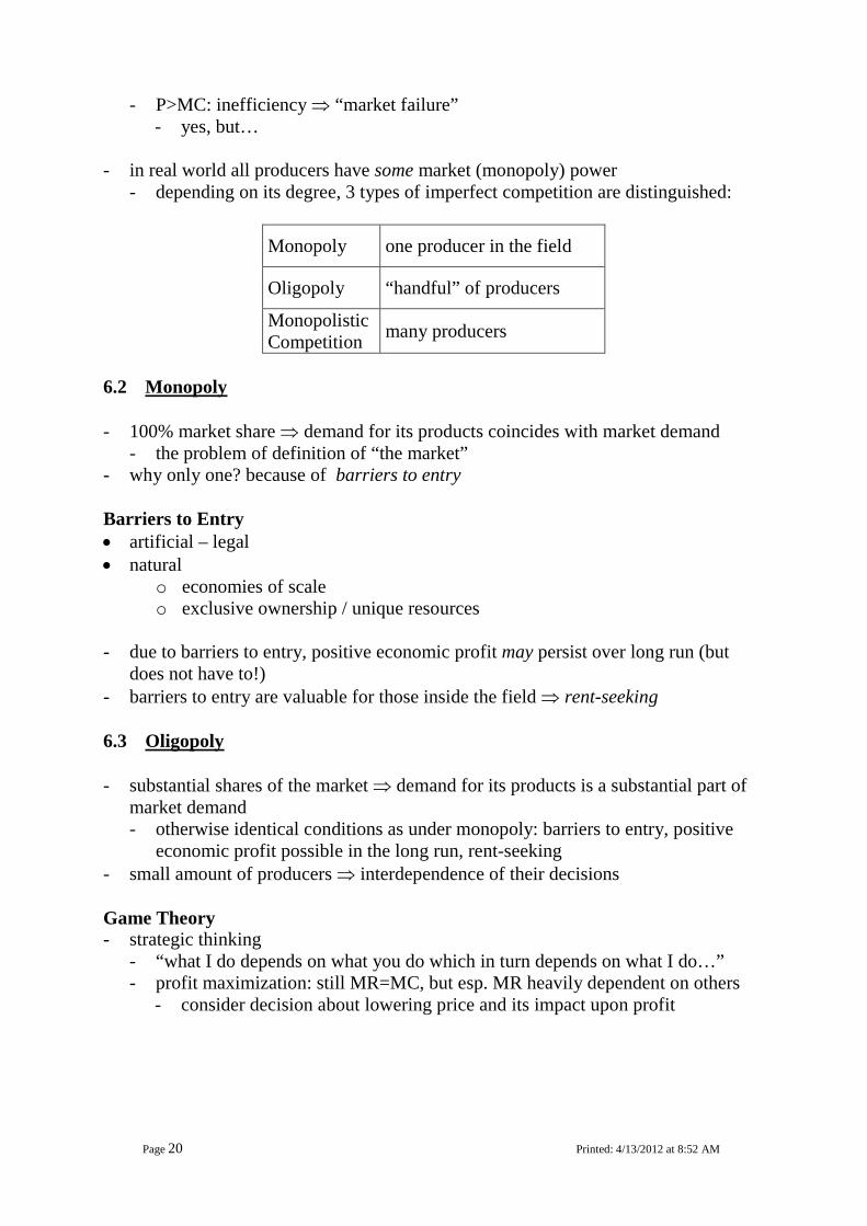
- depending on its degree, 3 types of imperfect competition are distinguished:

Monopoly one producer in the field

Oligopoly “handful” of producers

Monopolistic Competition many producers

6.2 Monopoly - 100% market share ⇒ demand for its products coincides with market demand

- the problem of definition of “the market” - why only one? because of barriers to entry Barriers to Entry • artificial – legal • natural

o economies of scale o exclusive ownership / unique resources

- due to barriers to entry, positive economic profit may persist over long run (but

does not have to!) - barriers to entry are valuable for those inside the field ⇒ rent-seeking 6.3 Oligopoly - substantial shares of the market ⇒ demand for its products is a substantial part of

market demand - otherwise identical conditions as under monopoly: barriers to entry, positive

economic profit possible in the long run, rent-seeking - small amount of producers ⇒ interdependence of their decisions Game Theory - strategic thinking

- “what I do depends on what you do which in turn depends on what I do…” - profit maximization: still MR=MC, but esp. MR heavily dependent on others

- consider decision about lowering price and its impact upon profit


Others

keep lower

I will

keep

m$ 2.0 m$ 3.0

m$ 2.0 m$ 0.2 lo

wer

m$ 0.2 m$ 0.6

m$ 3.0 m$ 0.6

- both have incentives to lower the price ⇒ both are worse off - they may gain by cooperating ⇒ cartels

- price-collusion - hard to practice as both have an incentive to cheat on the other

6.4 Monopolistic Competition - monopoly power but no barriers to entry ⇒ no economic profit in the long run

(normal profit only) - most markets


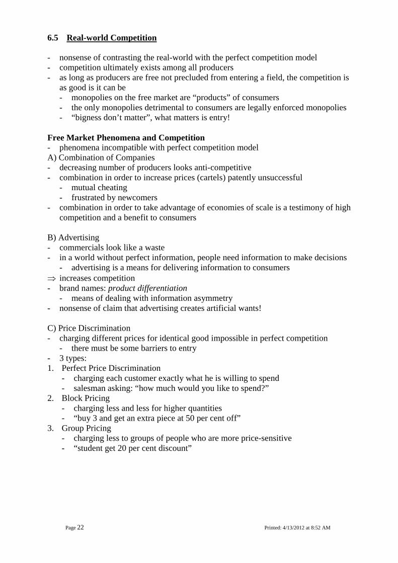
6.5 Real-world Competition - nonsense of contrasting the real-world with the perfect competition model - competition ultimately exists among all producers - as long as producers are free not precluded from entering a field, the competition is

as good is it can be - monopolies on the free market are “products” of consumers - the only monopolies detrimental to consumers are legally enforced monopolies - “bigness don’t matter”, what matters is entry!

Free Market Phenomena and Competition - phenomena incompatible with perfect competition model A) Combination of Companies - decreasing number of producers looks anti-competitive - combination in order to increase prices (cartels) patently unsuccessful

- mutual cheating - frustrated by newcomers

- combination in order to take advantage of economies of scale is a testimony of high competition and a benefit to consumers

B) Advertising - commercials look like a waste - in a world without perfect information, people need information to make decisions

- advertising is a means for delivering information to consumers ⇒ increases competition - brand names: product differentiation

- means of dealing with information asymmetry - nonsense of claim that advertising creates artificial wants! C) Price Discrimination - charging different prices for identical good impossible in perfect competition

- there must be some barriers to entry - 3 types: 1. Perfect Price Discrimination

- charging each customer exactly what he is willing to spend - salesman asking: “how much would you like to spend?”

2. Block Pricing - charging less and less for higher quantities - “buy 3 and get an extra piece at 50 per cent off”

3. Group Pricing - charging less to groups of people who are more price-sensitive - “student get 20 per cent discount”


Chapter 7 Input Markets

Outline: 7.1 Introduction 7.2 Demand for Inputs 7.3 Supply of Inputs 7.4 Supply of Labor and Labor Market 7.5 Supply of Land and Land Market 7.6 Financial Capital 7.1 Introduction - so far we have been concerned generally with goods used for consumption

(oranges, shoes, marijuana): goods that were the ultimate end of people’s desire - now it is time to extend our analysis to cover explicitly the inputs: goods that are

used to produce further goods - material (semi-finished goods) and other factors of production: land, labor,

capital goods - good news: we will use the same tools as we used for consumption good market

analysis - demand (embodying MU) and supply (embodying MC), determining

equilibrium price and quantity - we will follow the same steps as before

7.2 Demand for Inputs - recall the general concept of demand - 2 modifications:

1) concerning Q - by Quantity we mean quantity of services of the input, which is NOT

necessarily the same as the quantity of pieces of that input - material: no difference (coal, nails, wood: we use them “out of existence”) - durable goods: one machine is not the same as using the machine for an hour

- machine embodies all services that it is capable of rendering during its lifetime

- here we are concerned with unit of its service (e.g. 1 hour of working time) and its rental price ⇒ this is why we sometimes have a special term for the price of inputs,

by which we mean the price of its services - labor: wage - land: (ground) rent

- the price of the input as such will be dealt with in 7.6

2) concerning MU behind D - when talking about consumer goods, we assumed consumers have some

pleasure from the goods they demand: we gave it a name (utility) but did not further inquire about why it is so (we left this to psychology or other sciences)

- as inputs are demanded by producers, and as we assume the producers are maximizing profit, we know much more about why inputs are demanded:


- because of their productivity: factors of production produce something that can be sold for money (which is assumed to be the utility for producer) - the amount of money that will be gained by employing given input is

called its marginal revenue product (MRP) - it is the contribution of the given input to the total revenue from

selling the output - it can be figured out as marginal product (MP) of the input times the

marginal revenue (MR) from selling the output

MRP = MP*MR

General Concept of Demand

P

Q - it can be graphically derived from the marginal product curve

- factors influencing the quantity demanded QD ← Price of the input

← Preference, i.e. MRP

MP (productivity) MR (resp. POUTPUT) ← Productivity of other inputs

← Prices of other inputs

substitutes complements ← Expectations 7.3 Supply of Inputs - inputs are simply products of previous production - generally, not much of a difference compared to supply of consumer goods

o determined by MC o as for supply curve and its changes, see Chapter 3

D [MRP] 1) quantity of services, NOT physical quantity

2) special name for MU: marginal

revenue product




Input Market

P

Q - there are specific inputs which deserve special attention: labor and land 7.4 Labor Supply and Labor Market Labor Supply - supplied by workers, laborers (not demanded) - we assume labor is a pain, not a pleasure; something less preferable than leisure - labor is not everything that is associated with physical or mental activity (playing

tennis or scrabble is not labor, it is preferred to not doing anything: it is a consumer good…)

- why do people work then? o because of the reward they get for which they can buy goods that are

directly useful to them o decision of how much to work – how much work to “supply” – is based

on a trade-off between two goods: utility of leisure utility from consumption of the goods that can be obtained with

earned money - the more one works

- the more leisure he is giving up, and the more valuable leisure is - the more money he is earning, the more goods he can buy and the less valuable

is the goods ⇒ the more one works the higher the cost of working and the lower the benefits of

work - applying MU>MC

D [MRP]

S [MC]


Supply of Labor

w

L Labor Market - determining amount of hired labor and the reward – the wage - labor market regulation

- minimum wage laws - fringe benefits - working hours

- discrimination on labor market 7.5 Supply of Land and Land Market - the meaning of “land”: not only land, but anything that is given by nature - supply often assumed to be fixed - the land market

Market for Land

r

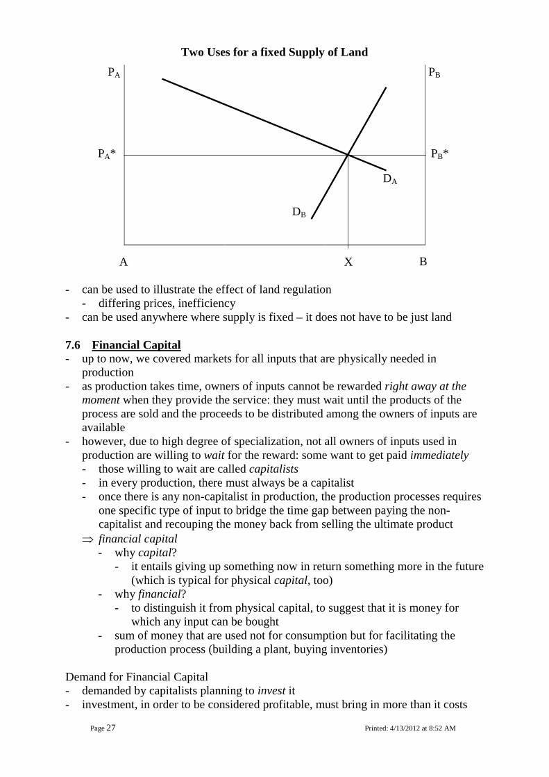
Land - assuming fixed supply of land, we can illustrate the effect of competing uses upon

the price on a graph that features only demand curves - distance AB shows the total available amount of land which will be used either

for A or for B - with given demands for A and B, the amount of land that will end up being

used for A is AX, and for B is XB - note that the prices in each use are equal

SL [MC of work = MU of leisure given up]

S

D

r*


Two Uses for a fixed Supply of Land

PA PB

- can be used to illustrate the effect of land regulation

- differing prices, inefficiency - can be used anywhere where supply is fixed – it does not have to be just land 7.6 Financial Capital - up to now, we covered markets for all inputs that are physically needed in

production - as production takes time, owners of inputs cannot be rewarded right away at the

moment when they provide the service: they must wait until the products of the process are sold and the proceeds to be distributed among the owners of inputs are available

- however, due to high degree of specialization, not all owners of inputs used in production are willing to wait for the reward: some want to get paid immediately - those willing to wait are called capitalists - in every production, there must always be a capitalist - once there is any non-capitalist in production, the production processes requires

one specific type of input to bridge the time gap between paying the non-capitalist and recouping the money back from selling the ultimate product

⇒ financial capital - why capital?

- it entails giving up something now in return something more in the future (which is typical for physical capital, too)

- why financial? - to distinguish it from physical capital, to suggest that it is money for

which any input can be bought - sum of money that are used not for consumption but for facilitating the

production process (building a plant, buying inventories) Demand for Financial Capital - demanded by capitalists planning to invest it - investment, in order to be considered profitable, must bring in more than it costs

X A B

PA* PB*

DB

DA


- the problems is however that revenues and costs occur at different times - it is impossible to compare the nominal values of costs TODAY with

revenues ONE YEAR FROM NOW ⇒ future streams of money must be converted into today’s terms, so that the

streams of money become comparable: this adjustment is called discounting - importance of time preference (preference of presence over future)

- the measure of it: the rate of time preference (rtp) - it is a subjective preference, specific to each individual (just as the

value of leisure or the preference for oranges or hotdogs is subjective and specific to everyone)

- the premium one puts on the present value in comparison to the future value - imagine e.g. a right to receive a $100 bill in exactly 1 year from

now; then we may ask different individuals about how much they value such a right now (i.e. how much would they spend now in order to acquire such a right)

- if somebody says that he would spend $80 at the max, it is clear that for him $80 now (80 present dollars) pretty much equals $100 a year from now (100 future dollars)

⇒ present dollars are more valuable than future dollars; how much more valuable? - 80 * (1 + rtp) = 100 - rtp = (100/80) -1 = 0.25 = 25 %

- today’s value of future income (benefits in general) can thus be found out by dividing the future value by (1+rtp) - such as in our case, $100 in the future with rtp=0.25 means 100/(1+0.25),

i.e. $80, today - when making investment decisions (demanding and using financial capital),

instead of individual rate of time preference, we use the market outcome of it, i.e. the interest rate (i)

⇒ in general, today’s value of x dollars to be paid in n years from now when the interest rate is i per cent:

x (1+i)n

- adjusting all money streams associated with given investment enables us to figure out the net present value (NPV) of given investment - positive means profitable investment - negative means a losing business

- the lower the interest rate (i), the more investment projects are deemed profitable and more investment funds are demanded

- determinants of quantity demanded:

QD ← i (–) ← Productivity (+)

← Expectations, Business Confidence (+/–)


Demand for Investment (Demand for Loanable

Funds)

i

financial capital Supply of Financial Capital - supplied by savers: people who do not spend money on consumption AND loan the

saving (only this can be invested in turn!) - determinants of quantity supplied:

QS ← i (+) ← Time preference (–) ← Expectations (+/–)

Supply of Savings

(Supply of Loanable Funds)

i

financial capital ⇒ Loanable Funds Market - determination of the interest rate 7.7 Capital Value - once we understand the determination of prices of services of inputs and

understand discounting, we are ready to understand the prices of whole inputs (land, machines, slaves)

D

S


- value of an input is determined by the value of all services over time that the input represents: their NPV

- even if the series of services is infinite, the value of the input is finite (unless the interest rate is zero) - perpetuity

NPV$X per year forever = X + X + … + X = X (1+i) (1+i)2 (1+i)∞ i

- e.g. how much would you pay for a right to receive $100 a year forever if the interest rate is 10 %?

NPV$100 per year forever with i=10% = 100 = 1000 0.1

Documents

MICROECONOMICS at UNYP Dan Stastny