Embed Size (px)
Citation preview

Principal - Agent model under moral hazardMicroeconomics 2
Presentation: Francis Bloch,Slides: Bernard Caillaud
Master APE - Paris School of Economics
March 16 (Lecture 12) and March 20 (Lecture 13), 2017
Presentation: Francis Bloch, Slides: Bernard Caillaud Principal - Agent model under moral hazard

I. Moral Hazard - I.1. Introduction
Principal - Agent model as the elementary block to build upmodels of transactions under asymmetric information
Principal, who lacks information, proposes a setting for thetransaction
Agent, who is informed, accepts or refuses the transactionsetting
If agreement, the transaction is implemented
Previously: incomplete information or screening, i.e. missinginformation on some exogenous parameters
Today: imperfect information or moral hazard, i.e. missing in-formation about some endogenous variables (Agent’s decisions)
Presentation: Francis Bloch, Slides: Bernard Caillaud Principal - Agent model under moral hazard
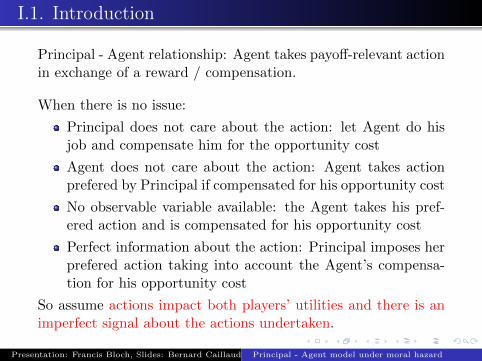
I.1. Introduction
Principal - Agent relationship: Agent takes payoff-relevant actionin exchange of a reward / compensation.
When there is no issue:
Principal does not care about the action: let Agent do hisjob and compensate him for the opportunity cost
Agent does not care about the action: Agent takes actionprefered by Principal if compensated for his opportunity cost
No observable variable available: the Agent takes his pref-ered action and is compensated for his opportunity cost
Perfect information about the action: Principal imposes herprefered action taking into account the Agent’s compensa-tion for his opportunity cost
So assume actions impact both players’ utilities and there is animperfect signal about the actions undertaken.
Presentation: Francis Bloch, Slides: Bernard Caillaud Principal - Agent model under moral hazard

I.1. Introduction
Wide applicability of moral hazard model:
Insurance company / insured agent
Employer / employee: provide incentives to the employee sothat he takes profit-enhancing actions that are costly to him
Shareholders / CEO: induce the manager to implement projectsthat enhance the firm value and not his own private benefits
Plaintiff / attorney: induce attorney to expend costly effortto increase plaintiff’s chances of prevailing at trial (also allexpertise relationships)
Homeowner / contractor: induce contractor to complete workon time by expending appropriate but costly effort
Landowner / farmer: induce farmer to grow crops and pre-serve soil quality, sharecropping...
Presentation: Francis Bloch, Slides: Bernard Caillaud Principal - Agent model under moral hazard

I.2. Road map for today
Canonical two-action model:
General presentation
Cost-minimizing contract implementing a given action
Optimal contract and inefficiency result
General (discrete) framework:
Existence and general inefficiency theorem
About monotonicity
Sufficient statistics theorem and information structures
Discussion: first-order approach, asymptotic efficiency
Dynamic issues: memory, savings
Applications:
Linear schemes in Holmstrom-Milgron: Multitask schemesand organizational design
Limited Liability models: Corporate finance
Presentation: Francis Bloch, Slides: Bernard Caillaud Principal - Agent model under moral hazard

I.2. Canonical setting
Transaction between Principal and Agent:
Agent takes a transaction-relevant action a ∈ A compact inR+, unobservable by any other party
Observable signal, i.e. random variable x ∈ X ⊂ R
a affects the signal: conditional cdf or proba (if finite) of xgiven a: Fa(x).
The other part of the transaction is an observable and con-tractable action by Principal: payment w ∈ R
Principal often assumed risk-neutral: V = x− wAgent’s risk-averse preferences: U = u(w)− C(a), u(.) con-cave increasing unbounded, C(.) convex increasing (separa-bility is a strong and important assumption)
Presentation: Francis Bloch, Slides: Bernard Caillaud Principal - Agent model under moral hazard

I.2. Canonical setting
Principal proposes a compensation mode, called a contract: spec-ifies how w is determined based on variables that can be observedwithout ambiguity by both parties and a lawyer who would en-force the contract
These variables are called verifiable, or contractible variables: acontract can be based on their specification
If Agent refuses, he obtains a reservation utility UR and Prin-cipal a reservation utility normalized to 0
If Agent accepts, then he decides a, outcome x arises andcontractual transfers are implemented
Presentation: Francis Bloch, Slides: Bernard Caillaud Principal - Agent model under moral hazard
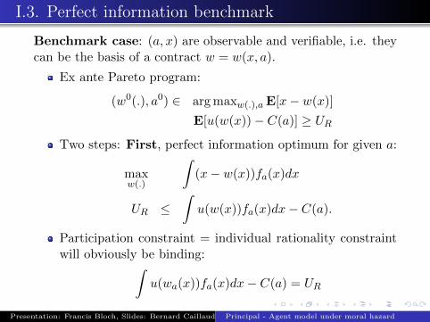
I.3. Perfect information benchmark
Benchmark case: (a, x) are observable and verifiable, i.e. theycan be the basis of a contract w = w(x, a).
Ex ante Pareto program:
(w0(.), a0) ∈ arg maxw(.),a E[x− w(x)]
E[u(w(x))− C(a)] ≥ URTwo steps: First, perfect information optimum for given a:
maxw(.)
∫(x− w(x))fa(x)dx
UR ≤∫u(w(x))fa(x)dx− C(a).
Participation constraint = individual rationality constraintwill obviously be binding:∫
u(wa(x))fa(x)dx− C(a) = UR
Presentation: Francis Bloch, Slides: Bernard Caillaud Principal - Agent model under moral hazard

I.3. Perfect information benchmark
Optimal risk-sharing in Pareto optimum: equalized MRSacross states (called Borch rule): u′(wa(x)) must be constantacross all x
That is: wa(x) = u−1(UR + C(a)), i.e. perfect insurance
In general (risk averse Principal), optimal risk sharing: 0 ≤w′a(x) ≤ 1
Second step is easy: maximize w.r.t. a
a0 = arg maxa
∫ (x− u−1(UR + C(a))
)fa(x)dx
Optimum: Principal proposes a forcing contract: you takeaction a0 and you’ll be paid w0(x) = u−1(UR + C(a0)) irre-spective of the outcome x: Full efficiency.
Presentation: Francis Bloch, Slides: Bernard Caillaud Principal - Agent model under moral hazard

I.4. First hint on imperfect information
Suppose now a not observable by Principal (or anybody else)
Perfect information optimum is action a0 and a constanttransfer w0 = u−1(UR + C(a0)) (risk-netrual Principal)
Faced with perfect information contract, Agent chooses hisaction
maxa
(u(w0)− C(a)
)= UR + C(a0)−min
aC(a) > UR
a ≡ minA: he chooses the minimal-cost effort, since he isperfectly insured !
Tension between optimal risk sharing (full insurance) and incen-tives to expend effort
Presentation: Francis Bloch, Slides: Bernard Caillaud Principal - Agent model under moral hazard

I.4. First hint on imperfect information
Suppose the Agent is risk-neutral: u(w) = w
Full information optimum yields profit for P:
Π = E[x | a0]− C(a0)− UR = maxa
(E[x | a]− C(a))− UR
Sell-out contract: w(x) = x−Π→Agent residual claimantof profits for purchase price of Π and chooses
maxa
(∫w(x)fa(x)dx− C(a)
)= max
a(E[x | a]− C(a)−Π)
= UR
for a = a0 ! He takes efficient action, full efficiency !
BUT with risk-aversion, this violates optimal risk-sharing
Fundamental conflict: Pareto efficiency vs incentives
Presentation: Francis Bloch, Slides: Bernard Caillaud Principal - Agent model under moral hazard

I.4. First hint on imperfect information
How much risk is necessary ? What is the optimal contract?
maxw(.),a
∫(x− w(x)) fa(x)dx
s.t. :
∫u(w(x))fa(x)dx− C(a) ≥ UR
and : a ∈ arg maxa′
(∫u(w(x))fa′(x)dx− C(a′)
)Agent accepts the contract: participation / IR constraint
New constraint = incentive constraint: the action induced isthe one preferred by the Agent to any other action a′ wihtinthe framework of the contract
Simplify this (too general) setting to get intuition
Presentation: Francis Bloch, Slides: Bernard Caillaud Principal - Agent model under moral hazard

II. Analysis in the basic model – II.1. Setting
Solving this problem may be tricky in general → Start with thebinary version with 2 actions: much of the intuition.
Effort can take 2 values: A = {0, 1}, C(1) = C > 0 = C(0)
Principal is risk neutral
Principal’s program under moral hazard solved in 2 stages
For a given a, what is the best contract that induces theAgent to take action a ? That is, what is the cost-minimizingcontract that implements aCompare the cost-minimizing contract that implements a = 1and the cost-minimizing contract that implements a = 0
NB: cost-minimizing contract that implements a = 0 is theperfect insurance contract w0 = u−1(UR)
Presentation: Francis Bloch, Slides: Bernard Caillaud Principal - Agent model under moral hazard

II.2. Cost-minimizing contract that implements a = 1
minw(.)
∫w(x)f1(x)dx
s.t. :
∫u(w(x))f1(x)dx− C ≥ UR
and :
∫u(w(x))f1(x)dx− C ≥
∫u(w(x))f0(x)dx
λ ≥ 0 multiplier associated to IR constraint
µ ≥ 0 multiplier associated to IC constraint
If µ = 0, solving without IC leads to w1 = u−1(UR + C),which induces Agent to choose a = 0 ! So, µ > 0
IR binding; otherwise, consider dw(x) such that, for all x
u(w(x))− u(w(x) + dw(x)) = ε > 0
Presentation: Francis Bloch, Slides: Bernard Caillaud Principal - Agent model under moral hazard

II.2. Cost-minimizing contract that implements a = 1
Optimizing the Lagrangean, FOC:
1
u′(w∗1(x))= λ+ µ
(1− f0(x)
f1(x)
)= λ+ µ (1− r(x))∫
u(w∗1(x))f1(x)dx− C = UR∫u(w∗1(x))f1(x)dx− C =
∫u(w∗1(x))f0(x)dx
where r(x) is the likelihood ratio f0(x)f1(x)
r(x) measures how likely it is that x comes from a draw from(x | a = 0) compared to a draw from (x | a = 1)
Compensation w∗1(x) is higher (lower) when the likelihoodratio is lower (higher), i.e. when it is relatively likely (un-likely) that Agent has chosen a = 1 (a = 0)
Presentation: Francis Bloch, Slides: Bernard Caillaud Principal - Agent model under moral hazard

II.2. Cost-minimizing contract that implements a = 1
Does compensation increase in performance x (w∗1(.) increasing)?
1
u′(w∗1(x))= λ+ µ (1− r(x))
YES iff r(x) is decreasing in x, i.e. if higher performancegives more confidence that a = 1 has been chosen ! (MLRP,Monotone likelihood ratio property)
NO in general !
See the counter-example on the picture below
Presentation: Francis Bloch, Slides: Bernard Caillaud Principal - Agent model under moral hazard
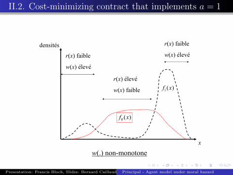
II.2. Cost-minimizing contract that implements a = 1
�
��� ��
��� ��
���������
������� �
������� �
���������
���������
������� �
��������
�����������������
Presentation: Francis Bloch, Slides: Bernard Caillaud Principal - Agent model under moral hazard
II.2. Cost-minimizing contract that implements a = 1
The nature of the problem is stochastic: stochastic link from ato x matters, not physical link
In fact, there is nothing special about x except that it is anobservable signal about the action; could be different from Prin-cipal’s gross profit.
Note also that MLRP implies FOSD, i.e. F1(w) ≤ F0(x) for allx, but the reverse is not true.
Necessary that effort stochastically increases output for theoptimal compensation to increase in performance
But not sufficient !
Presentation: Francis Bloch, Slides: Bernard Caillaud Principal - Agent model under moral hazard

II.2. Cost-minimizing contract that implements a = 1
If several signals about Agent’s action, which one to use ?
Two verifiable signals: (x, y) ∼ fa(x, y)
FOC are similar:
1
u′(w∗1(x, y))= λ+ µ
(1− f0(x, y)
f1(x, y)
).
w∗1(x, y) iff r(.) depends on x and on y
A contrario, suppose fa(x, y) = k(x, y)ga(x), then r(.) de-pends only on x and w∗1(.) should not depend on y optimally.
fa(x, y) = k(x, y)ga(x) ⇔ x is a sufficient statistics on afor the pair (x, y), i.e. y does not convey any additionalinformation on a that is not already contained in x
This is the sufficient statistics theorem (Holmstrom)
Presentation: Francis Bloch, Slides: Bernard Caillaud Principal - Agent model under moral hazard
II.3. Optimal contract
Cost-minimizing contract that implements a = 1 is morecostly due to imperfect information on a:∫
w∗1(x)f1(x)dx > u−1(UR + C)
Principal’s net profit of inducing a = 1 is smaller than per-fect information profits:∫
(x− w∗1(x)) f1(x)dx <
∫xf1(x)dx− u−1(UR + C)
Even if a = 1 is optimal under perfect information, a = 0may become optimal under imperfect information on a
Cost of moral hazard
Moral hazard implies a strict loss for the Principal: either inducea = 1 at a larger cost, or induce a = 0.
Presentation: Francis Bloch, Slides: Bernard Caillaud Principal - Agent model under moral hazard
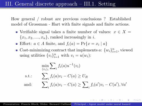
III. General discrete approach – III.1. Setting
How general / robust are previous conclusions ? Establishedmodel of Grossman - Hart with finite signals and finite actions.
Verifiable signal takes a finite number of values: x ∈ X ={x1, x2, ...., xn}, ranked increasingly in i.
Effort: a ∈ A finite, and fi(a) = Pr{x = xi | a}Cost-minimizing contract that implements a: {wi}ni=1, viewedusing utilities {vi}ni=1 with vi = u(wi):
min(vi)i
∑ifi(a)u−1(vi)
s.t.:∑
ifi(a)vi − C(a) ≥ UR
and:∑
ifi(a)vi − C(a) ≥
∑ifi(a
′)vi − C(a′), ∀a′
Presentation: Francis Bloch, Slides: Bernard Caillaud Principal - Agent model under moral hazard

III.2. General results
All constraints are linear constraints, u−1(.) is convex; standardpolygonal program where the only problem is whether the set ofconstraints is empty.
Definition of an implementable action
a is implementable if the set of constraints is not empty
Proposition: Binding participation constraint
If a implementable, participation constraint binds at cost-minimizing contract that implements a
Proof: If not, consider a uniform decrease in vi, ∀i.This result depends on Agent’s utility being additively sep-arable in money / action
OK with multiplicatively separable: u(w)γ(a) (check it!)
Presentation: Francis Bloch, Slides: Bernard Caillaud Principal - Agent model under moral hazard

III.2. General results
Existence of cost-minimizing contract iff set of constraints is notempty, i.e. a implementable
Proposition: Condition of implementability / existence
a implementable iff there does not exists a distribution ν(a′) overa′ ∈ A \ {a}, such that: for any i∑
a′ 6=aν(a′)fi(a
′) = fi(a) and∑a′ 6=a
ν(a′)C(a′) < C(a)
Proof: existence of a solution to set of IC inequalities, relatedto Farkas’ Lemma (Theorem 22.1, Rockafellar 1970)
Intuition: no way to achieve the same distribution over out-comes at smaller (expected) cost.
Presentation: Francis Bloch, Slides: Bernard Caillaud Principal - Agent model under moral hazard

III.2. General results
Cases where moral hazard does not matter:
a can be implemented at the same cost as under perfectinformation (with perfect insurance contract)
The case of shifting support:
Distribution fi(.)i has shifting support relative to a if thereexists i0 such that fi0(a) = 0 < fi0(a′) for all a′ such thatC(a′) < C(a)If the distribution has shifting support relative to a, a can beimplemented at the same cost as under perfect informationIntuition: take vi0 → −∞ (assumption u(.) unbounded frombelow) and vi = UR + C(a) otherwise
If Agent is risk neutral
Presentation: Francis Bloch, Slides: Bernard Caillaud Principal - Agent model under moral hazard

III.2. General results
General loss for the Principal due to moral hazard
Assume a implementable, u(.) stricly concave, fi(.)i has full sup-port and C(a) > mina′∈AC(a′), cost of implementing a undermoral hazard is strictly higher than under perfect information.
Proof:
Cannot be smaller: more constraints
Under the assumptions, there exists i, j such that vi 6= vj
So, Jensen inequality + concavity + full support yield:
∑k
fk(a)u−1(vk) > u−1
(∑k
fk(a)vk
)≥ u−1 (UR + C(a))
Presentation: Francis Bloch, Slides: Bernard Caillaud Principal - Agent model under moral hazard

III.3. Further results about monotonicity
Monotonic properties of cost-minimizing contract
Assume previous assumptions:
there exists i such that wi < wi+1
there exists j such that xj − wj < xj+1 − wj+1
Very weak properties ! Going further with Kuhn-Tucker?
1
u′(u−1(vi))=
λ+∑a′ 6=a
µ(a′)
−∑a′ 6=a
µ(a′)fi(a
′)
fi(a)
with µ(a′) > 0 means Agent is indifferent between a and a′
Presentation: Francis Bloch, Slides: Bernard Caillaud Principal - Agent model under moral hazard

III.3. Further results about monotonicity
At optimum, there exists (at least) one such less costly actiona′ for which µ(a′) > 0
If there exists just one such a′, as in the two-action model.
MLRP hypothesis: For all (a, a′) ∈ A2, if C(a′) ≤ C(a) thenfi(a
′)fi(a)
is decreasing in i
Then, the cost-minimizing contract is increasing in i underMLRP
But if there exists a′ and a” with C(a′) < C(a) < C(a”),µ(a′) > 0 and µ(a”) > 0, MLRP does NOT imply that:
µ(a′)fi(a
′)
fi(a)+ µ(a”)
fi(a”)
fi(a)decreases in i
Presentation: Francis Bloch, Slides: Bernard Caillaud Principal - Agent model under moral hazard

III.3. Further results about monotonicity
Spanning condition: There exists two distributions fi
and fi
over X, with fifi
decreasing in i and non-decreasing mapping
λ(.) from A to [0, 1] such that:
∀a, fi(a) = λ(a)fi + (1− λ(a))fi
Spanning condition is sufficient for monotonicity, but strong
CDFC assumption: For all (a, a′, a”) such that C(a) = λC(a′)+(1− λ)C(a”), the following holds:
F (· | a) �FOSD λF (· | a′) + (1− λ)F (· | a”)
MLRP + CDFC are sufficient conditions for monotonicity,but again quite strong
Conclusion: monotonicity is not a natural property in themoral hazard framework
Presentation: Francis Bloch, Slides: Bernard Caillaud Principal - Agent model under moral hazard

III.4. Information structures
In two-effort setting: a glimpse on when one should make thecompensation contingent on an additional signal and when not.
General link between information structures (signal technologies)and Principal’s cost of implementing a given action a under moralhazard ?
A moral hazard environment is characterized by the informationstructure, summarized by f(.) from A into a simplex
Question: compare the expected compensation to implementaction a (i.e. moral hazard cost of implementing a) under infor-mation structure f(.) (vector of dim n) and information structureg(.) (of dim m) ?
Presentation: Francis Bloch, Slides: Bernard Caillaud Principal - Agent model under moral hazard

III.4. Information structures
Let Γ(a; f) denote the value of the cost-minimizing program thatimplements action a when the structure of verifiable signals isgiven by f(.)
Compare Γ(.; f) and Γ(.; g) for two signal technology f(.) andg(.).
Recall a basic definition:
Blackwell sufficient information structures
f(.) (of dim n) is sufficient for g(.) (of dim m) in the sense ofBlackwell if there exists a transition matrix P (of dim m × n)such that: g(.) = P.f(.) (i.e. gj(.) =
∑i pjifi(.))
Presentation: Francis Bloch, Slides: Bernard Caillaud Principal - Agent model under moral hazard

III.4. Information structures
Comparison of information structures
If f(.) (of dim n) is sufficient for g(.) (of dim m) in the sense ofBlackwell, then Γ(.; f) ≤ Γ(.; g).
Proof:
vj : cost-min contract under g(.) and let define a contract uibased on signal f(.) as: ui =
∑j pjivj (or u = P t.v)
Sufficiency implies for any action α, g(α)t.v = f(α)t.P t.v =f(α)t.u, so that u satisfies also (IC) and (IR)
New contract is cheaper than original one (Jensen again):
∑i
fi(a)u−1(ui) =∑i
fi(a)u−1
∑j
pjivj
≤
∑ij
fi(a)pjiu−1(vj) =
∑j
gj(a)u−1(vj)
Presentation: Francis Bloch, Slides: Bernard Caillaud Principal - Agent model under moral hazard

III.4. Information structures
Getting back: suppose there are 2 signals, x ∈ {x1, x2, ..., xi, ...xn},characterized by (marginal) fi(.), and y ∈ {y1, y2, ..., yj , ...ym},characterized by (joint) hij(.) for i = 1, 2, .., n and j = 1, 2, ...,m.
In general, Principal will incur a smaller moral hazard cost ofimplementing any action (except lowest cost one) if he makes thecompensation contingent on both x and y.
Proof:
Let gk(.) = hij(.) for k = (i− 1)m+ j, k = 1, ..., nm.
With P such that pik = 1 if and only if k ∈ {(i−1)m+1, (i−1)m+ 2, ..., im} and 0 otherwise, g(.) sufficient for f(.):
fi(a) =∑j
hij(a) =
im∑k=(i−1)m+1
gk(a) =∑k
pikgk(a)
Presentation: Francis Bloch, Slides: Bernard Caillaud Principal - Agent model under moral hazard
III.4. Information structures
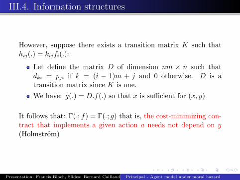
However, suppose there exists a transition matrix K such thathij(.) = kijfi(.):
Let define the matrix D of dimension nm × n such thatdki = pji if k = (i − 1)m + j and 0 otherwise. D is atransition matrix since K is one.
We have: g(.) = D.f(.) so that x is sufficient for (x, y)
It follows that: Γ(.; f) = Γ(.; g) that is, the cost-minimizing con-tract that implements a given action a needs not depend on y(Holmstrom)
Presentation: Francis Bloch, Slides: Bernard Caillaud Principal - Agent model under moral hazard

III.4. Information structures
Application:
A salesman’s effort aims at convincing buyers to buy thefirm’s product. When he visits a buyer, the buyer may endup signing up for a pre-order
Then macroeconomic shocks impact buyers’ budget and abuyer cancel his order before actual delivery (and payment)
(nb orders, nb sales) jointly distributed depending on effort,but the distribution of sales conditional on orders only de-pend on macroeconomic shocks
Observed performance: number of units ordered and numberof units actually sold
Salesman’s compensation should only depend on the ob-served number of orders, not on the observed sales as macroshocks are not informative about the salesman’s effort
Presentation: Francis Bloch, Slides: Bernard Caillaud Principal - Agent model under moral hazard
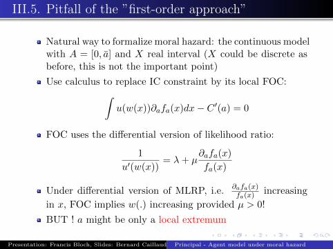
III.5. Pitfall of the ”first-order approach”
Natural way to formalize moral hazard: the continuous modelwith A = [0, a] and X real interval (X could be discrete asbefore, this is not the important point)
Use calculus to replace IC constraint by its local FOC:∫u(w(x))∂afa(x)dx− C ′(a) = 0
FOC uses the differential version of likelihood ratio:
1
u′(w(x))= λ+ µ
∂afa(x)
fa(x)
Under differential version of MLRP, i.e. ∂afa(x)fa(x) increasing
in x, FOC implies w(.) increasing provided µ > 0!
BUT ! a might be only a local extremum
Presentation: Francis Bloch, Slides: Bernard Caillaud Principal - Agent model under moral hazard

III.5. Pitfall of the ”first-order approach”
Weak local IC:∫u(w(x))∂afa(x)dx− C ′(a) ≥ 0
Then µ ≥ 0 and, as before, FOC imply w(.) increasing underdifferential version of MLRP
Differential CDFC: Fa(x) is convex in a for all x.
∂2aa
(∫u(w(x))fa(x)dx− C(a)
)= ∂2
aa
(−∫u′(w(x))w′(x)Fa(x)dx− C(a)
)= −
∫u′(w(x))w′(x)∂2
aaFa(x)dx− C”(a) ≤ 0
Agent’s objectives are concave, first-order approach OK; butrestrictive assumptions (MLRP + CDFC) as in discrete case
Presentation: Francis Bloch, Slides: Bernard Caillaud Principal - Agent model under moral hazard

III.6. Asymptotic perfect information optimum
We’ve considered X an interval or even R; when the densityvanishes, situation looks like a shifting support
Suppose x = a+ε, with ε distributed according to F (.) cont.diff. unimodal with zero mean.
Take a = [0, 1], C(a) = a2/2, u(0) = 0 = UR
Suppose full information optimum is: a = 1, v0 = 1/2
Consider the following threshold contract: for a given b,v(x) = v− if x < b and v(x) = v+ if x ≥ bAgent’s objectives:
max0≤a≤1
(F (b− a)v− + (1− F (b− a))v+ −
a2
2
)If (v+ − v−)f(b − 1) = 1 and f ′(b − 1) > 0, Agent choosesa = 1
Presentation: Francis Bloch, Slides: Bernard Caillaud Principal - Agent model under moral hazard
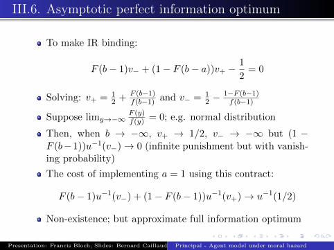
III.6. Asymptotic perfect information optimum
To make IR binding:
F (b− 1)v− + (1− F (b− a))v+ −1
2= 0
Solving: v+ = 12 + F (b−1)
f(b−1) and v− = 12 −
1−F (b−1)f(b−1)
Suppose limy→−∞F (y)f(y) = 0; e.g. normal distribution
Then, when b → −∞, v+ → 1/2, v− → −∞ but (1 −F (b−1))u−1(v−)→ 0 (infinite punishment but with vanish-ing probability)
The cost of implementing a = 1 using this contract:
F (b− 1)u−1(v−) + (1− F (b− 1))u−1(v+)→ u−1(1/2)
Non-existence; but approximate full information optimum
Presentation: Francis Bloch, Slides: Bernard Caillaud Principal - Agent model under moral hazard
IV. Dynamic issues – IV.1. Why study dynamics andhow?
Moral hazard models are widely used to model organizations,firms,... and these are long-lasting institutions: nexus of con-tracts for repeated interactions.
Similarly, contractual arrangements in markets (distribution andretailing, insurance, credit...) span over long time periods duringwhich several transactions take place.
Sources of dynamics:
Agent takes actions today, tomorrow,...
Information changes over time
The contractual setting is modified: related to commitmentissues
Presentation: Francis Bloch, Slides: Bernard Caillaud Principal - Agent model under moral hazard

IV.1. Why study dynamics and how?
Commitment = capacity to tie one’s own hands
Long term contract proposed once and for all;
Principal does not play after contract signature: no non-contractible action
Principal commits not to use information if it was not ex-plicitly stated in original contract
Abide by (possibly) ex-post (.i.e once some information hasbeen learnt) inefficient rules
This is a strong assumption. Alternative settings:
Absence of commitment: Principal and Agent repeatedlynegotiate spot contracts.
Commitment with renegotiation: parties can agree tomodify a long-term contract if it is mutually beneficial.
Presentation: Francis Bloch, Slides: Bernard Caillaud Principal - Agent model under moral hazard

IV.1. Why study dynamics and how?
Classical argument: Commitment is always (weakly) benefi-cial in a simple Principal - Agent relationship.
Proof: Principal committing to her equilibrium strategy in a non-commitment setting makes her as well off as without commiting,and Agent’s best response unchanged.
How necessary is the possibility of commitment ? Possible prop-erties of optimal long term contract:
Sequential efficiency, renegotiation-proof: At any date,no other mechanism and attached equilibrium that is mutu-ally beneficial for Principal (strictly) and Agent
Sequential optimality, replication by spot contracts:Sequential efficient and, at any date, Agent gets his reserva-tion utility
Presentation: Francis Bloch, Slides: Bernard Caillaud Principal - Agent model under moral hazard

IV.1. Why study dynamics and how?
Complete study of dynamics of moral hazard models beyondscope of this introductory course !
Focus on a few properties of the optimal long term contract in onePrincipal - one Agent framework with two periods to accountfor several transactions, actions, steps of information accrual, andone possible contractual change
Themes:
Role of memory
Agent’s access to financial markets
Observable but not verifiable actions
Presentation: Francis Bloch, Slides: Bernard Caillaud Principal - Agent model under moral hazard

IV.2. The role of memory in repeated moral hazard
t = 1 t = 2
a0 ∈ A (xi, wi)
Prob: fi(a0)
ai ∈ A(if xi)
(xj , wij)
Prob: fj(ai)
Standard model with X discrete and A continuum
Agent’s discount factor δ; risk-neutral Principal’s discountfactor is market discount factor ρ = 1
1+r
Technological separability: at t, output only determinedby current effort
a0 action implemented at 1st period, if observed outcomeat 1st period is xi, let ai denote the action implemented in2nd period (in general, incentives may induce a different 2ndperiod action depending on verifiable variables at 1st period)
Presentation: Francis Bloch, Slides: Bernard Caillaud Principal - Agent model under moral hazard

IV.2. The role of memory in repeated moral hazard
Contracts:
Compensation at t contingent on realized states of nature,i.e. on past and current outputs
wi or vi = u(wi) if xi at t = 1 and wij or vij = u(wij) if xiat t = 1 and xj at t = 2
Static benchmark (assume FO approach for simplicity):
Cost-minimizing condition for a:
1
u′(wi)= λ+ µ
f ′i(a)
fi(a)
Binding IR: ∑i
pi(a)vi − C(a) = U.
Presentation: Francis Bloch, Slides: Bernard Caillaud Principal - Agent model under moral hazard
IV.2. The role of memory in repeated moral hazard
Role of memory in optimal long term contract
The optimal LT contract exhibits memory provided moral hazardis not degenerate, i.e. if a0 is not the least costly action; moreprecisely, for i 6= i′, wi 6= wi′ implies ∃j, wij 6= wi′j .
Proof:
Suppose i 6= i′ such that: vi 6= vi′ .
If for all j, vij = vi′j = vj , then necessarily: ai = ai′ = a;i.e. same action induced (mild caveat if equivalent actions).
After xi at t = 1, modify: reduce vi− ε and after xj at t = 2for all j, increase vj + ε
δ :
incentives for 2nd period action after xi unchanged;Agent’s intertemporal utility if xi unchanged;obviously idem after any other observation
Presentation: Francis Bloch, Slides: Bernard Caillaud Principal - Agent model under moral hazard
IV.2. The role of memory in repeated moral hazard
Optimal intertemporal smoothing for Principal implies:
{ε = 0} = arg min{u−1(vi − ε) + ρ∑j
fj(a)u−1(vj +ε
δ)}
⇒ 1
u′(wi)=ρ
δ
∑j
fj(a)1
u′(wj)=
1
u′(wi′)⇒ wi = wi′
Contradiction: memory of first-period incentives
If no memory at all, it means that vi independent of i anda0 is the lowest-cost action.
Therefore, the optimal compensation must depend upon presentand past performance for the optimum contract, even thoughpast effort has no impact on current (or future) performance.
Presentation: Francis Bloch, Slides: Bernard Caillaud Principal - Agent model under moral hazard

IV.2. The role of memory in repeated moral hazard
As a consequence, the optimal LT contract is not sequentiallyoptimal
The period 2 utility provided by the optimal contract dependsupon the realization of xi at t = 1, hence cannot be equal to theexogenous reservation utility of the Agent.
However, the optimal LT contract is sequentially efficient (rene-gotiation proof):
If not, after history xi, replace branch of the LT contractby a better sub-contract, subject to the same continuationutility: U i ≡
∑j fj(ai)vij − C(ai).
Continuation utility constraint is binding: same expectedutility after xi.
Idem after other xi′
Hence, a better LT contract: contradiction.
Presentation: Francis Bloch, Slides: Bernard Caillaud Principal - Agent model under moral hazard

IV.3. Role of financial markets
In same framework, suppose the Agent has access to financialmarkets and can save (or borrow if negative) Si on his compen-sation wi after xi so as:
max{u(wi − Si) + δ∑j
fj(ai)u (wij + (1 + r)Si)}
Around Si = 0, A would like to save:
Derivates around Si = 0: −u′(wi)+δ(1+r)∑
j fj(ai)u′(wij)
Using same intertemporal transfer as in previous subsection:
1
u′(wi)=ρ
δ
∑j
fj(ai)1
u′(wij)
The function 1/x being convex, Jensen inequality implies:
δ(1+r)∑j
fj(ai)
(1/u′(wij))≥ δ(1+r)
∑j
fj(ai)
u′(wij)
−1
= u′(wi)
Presentation: Francis Bloch, Slides: Bernard Caillaud Principal - Agent model under moral hazard
IV.3. Role of financial markets
This is problematic: Agent can easily undo the incentives builtin the LT contract !!
One could think of limiting the borrowing possibilities of theAgent, but it seems hard to limit his saving possibilities !
Nevertheless, if savings are observable and verifiable, i.e. control-lable, they should also be included in the optimal moral hazardcontract:
min(wi,wij ,Si)
∑i,j
fi(a0)fij(ai)(wi + ρwij)
subject to IR and incentives constraints using∑i,j
fi(a0)fij(ai) [u(wi − Si) + δu(wij + (1 + r)Si)− C(a0)− δC(ai)]
Presentation: Francis Bloch, Slides: Bernard Caillaud Principal - Agent model under moral hazard

IV.3. Role of financial markets
With ci = wi−Si, cij = wij + (1 + r)Si, i.e. substitute consump-tion to earnings, same program as without financial markets:
Optimal LT contract with controlled access to financial markets
Consumption in optimal contract does not depend upon the (con-trolled) access to financial market; it exhibits memory and opti-mal LT contract with controlled savings is sequentially efficient.
Stronger result: sequential optimality
Optimal contract with controlled access is sequentially optimal
Key: at t = 2, IR depends upon accumulated savings SiUsing Si, adjust reservation utility (depends on savings) andmaintain unchanged continuation utility !
Access to financial markets disconnects the intertemporal smooth-ing problem from the moral hazard problems (incentives vs in-surance) at each t.
Presentation: Francis Bloch, Slides: Bernard Caillaud Principal - Agent model under moral hazard

IV.3. Role of financial markets
When savings cannot be fixed within the contract: savings be-come one additional moral hazard variable!
Sequential efficiency
In general, the optimal LT contract with non-controlled access tofinancial market is not sequentially efficient; hence not sequen-tially optimal.
In the usual proof of renegotiation-proofness (see earlier), whenone replaces one branch after xi with a better sub-contract, thisleaves expected utility unchanged but expected marginal utilitiesmay change through wealth effects, which conflicts with intertem-poral smoothing
Noticeable case: When u(w, a) = − exp{−r(w − c(a))}, util-ity and marginal utility are aligned: optimal LT is sequentiallyefficient.
Presentation: Francis Bloch, Slides: Bernard Caillaud Principal - Agent model under moral hazard
IV.4. Renegotiation after a signal
Not the same dynamics setting here, but issue is intrinsicallydynamic: what happens if the Agent’s action is observable tothe Principal, but not verifiable? Or if some observable butnon-verifiable signal is observed ?
One cannot write a contract based on this signal, but after ob-serving it, the Principal and the Agent can figure out what kindof contracts would now be better and renegotiate on such a con-tract !
In the one-period model with risk-neutral Principal, assume that:
After action a is taken and before outcome x is observed,both Principal and Agent observe signal s
and Principal and Agent can renegotiate on a new contractif mutually beneficial
Presentation: Francis Bloch, Slides: Bernard Caillaud Principal - Agent model under moral hazard

IV.4. Renegotiation after a signal
Simple case: the signal s is the action a and Principal hasbargaining power at renegotiation stage.
Observing the action:
Any implementable action under standard moral hazard is imple-mentable at full information cost u−1(C(a)) under renegotiation.
Proof:
After any a, gains from trade since risk is not optimallyshared and action is already decided: Principal offers newfixed compensation:
u−1(∑i
fi(a)vi)
Agent is indifferent
(IR) implies this is equal to u−1(C(a)).
Presentation: Francis Bloch, Slides: Bernard Caillaud Principal - Agent model under moral hazard

IV.4. Renegotiation after a signal
Renegotiation reduces the cost of implementable action down toits full information value. Therefore, the full information opti-mal action (if implementable) can be implemented under moralhazard with observability of action and renegotiation !
Renegotiaton is strictly valuable for Principal (if no shifting sup-port)
Compensation is not determined by the initial contract but bythe renegotiated contract. Initial contract serves as a threat pointif the Agent were to deviate.
Presentation: Francis Bloch, Slides: Bernard Caillaud Principal - Agent model under moral hazard
IV.4. Renegotiation after a signal
Other simple case: the signal s is the action a and Agent hasbargaining power at renegotiation stage.
The full information outcome is attainable here, too:
Consider the contract wi = xi−Π0, sell out contract at priceequal to the Principal’s full information profit.
At renegotiation avec a, Agent proposes full insurance atwage w such that: ∑
i
fi(a)xi − w = Π0
So, Agent expects:∑
i fi(a)u(wi) − C(a) =∑
i fi(a)xi −C(a)− Π0 which is maximized by definition for a = a0 andyields expected utility equal to the reservation value.
Presentation: Francis Bloch, Slides: Bernard Caillaud Principal - Agent model under moral hazard

IV.4. Renegotiation after a signal
Original contract determines the default payoff in the renegotia-tion, hence here the Principal’s profit.
Since renegotiation will bring back full insurance for the Agent,he can behave as if risk-neutral; hence the sell out contract.
This type of result extends to more balanced (but monotonic)renegotiation bargaining processes between Principal and Agent,provided the Principal keeps the bargaining power at the initialstage.
Presentation: Francis Bloch, Slides: Bernard Caillaud Principal - Agent model under moral hazard

IV.4. Renegotiation after a signal
More elaborate case: s is an imperfect signal and Principalhas all bargaining power.
Signal s ∈ {s1, ..., sj , ..., sm} with marginal probability gj(a).
Conditional probability of xi given a and sj : σij(a)
f(.) = Σ(.).g(.)
Principal knows s while Agent knows a and s: renegotiation po-tentially under incomplete information.
Except if Σ(a) = Σ(a′) for any two actions: i.e. if s is a sufficientstatistics about x for (s, a). Then, renegotiation under symmetricinformation.
Presentation: Francis Bloch, Slides: Bernard Caillaud Principal - Agent model under moral hazard

IV.4. Renegotiation after a signal
Under sufficient statistics assumption, renegotiation of a contractv leads to a full insurance contract at wage u−1(
∑i σijui) after
signal sj , and therefore to an expected utility for Agent:∑j
gj(a)∑i
σijui − C(a) =∑i
fi(a)ui − C(a)
So, the same IC and IR constraints hold with or without renego-tiation ! The set of implementable actions is the same
And if there is no shifting support for the signal, i.e. Σ >> 0,then the cost of implementing any action (but the least-cost one)is strictly smaller with renegotiation than without.
Without sufficient statistics condition: see Hermalin-Katz
Presentation: Francis Bloch, Slides: Bernard Caillaud Principal - Agent model under moral hazard

V. Applications
Remark about general moral hazard models:
General results about inefficiency and informativeness canbe obtained in the general framework
But it is difficult to obtain explicitly optimal contract and,consequently, almost impossible to use general moral hazardmodels in more complicated environments.
Applying moral hazard to understand organizations or manage-rial compensation schemes implies to make additional assump-tions so as to work with tractable models, with explicit solutions.
In this section:
Model with continuum of actions and outcomes and linearschemes
Model with risk neutrality ... but limited liability.
Presentation: Francis Bloch, Slides: Bernard Caillaud Principal - Agent model under moral hazard

V.1. Linear schemes with CARA utility
Holmstrom - Milgrom setting:
Agent takes multiple actions: a = (a1, ..., an) ∈ Rn+ at cost
C(a) convex
Principal’s benefit can be general (concave) B(a)
Agent’s actions generate a vector of signals: x = µ(a) + ε,where ε is normally distributed with zero mean and var/covmatrix Σ
Principal is risk neutral
Agent’s preferences: U(ω) = − exp{−rω} with ω is theAgent’s wealth: ω = w(x)− C(a)
Presentation: Francis Bloch, Slides: Bernard Caillaud Principal - Agent model under moral hazard

V.1. Linear schemes with CARA utility
Central assumption: we restrict attention to linear schemes,i.e. w(x) = αt.x+ β.
With linear contracts and normally distributed noise term, onehas:
E[U(w(µ(a) + ε)− C(a)] = U(αt.µ(a) + β − C(a)− r
2αt.Σ.α
)That is, one can reason in terms of certainty equivalent, equal tothe expected net wealth minus a risk premium.
The joint surplus to be maximized is: B(a) − C(a) − r2α
t.Σ.αwhich is independent of β. β simply determines the distributionof the joint surplus between both players.
Presentation: Francis Bloch, Slides: Bernard Caillaud Principal - Agent model under moral hazard

V.1. Linear schemes with CARA utility
Optimal contract program:
maxa,α {B(a)− C(a)− r
2αt.Σ.α}
s.t. a ∈ arg maxe{αtµ(e)− C(e)}
Assume that µ(a) = a so that we can follow a FO approach: theincentive constraint writes: α = ∂C(a) (for interior a >> 0)
FOC for the optimal contract are thus:
∂B(a)− [In + r∂2C(a).Σ].∂C(a) = 0
α = ∂C(a)
Presentation: Francis Bloch, Slides: Bernard Caillaud Principal - Agent model under moral hazard

V.1. Linear schemes with CARA utility
First consider the case of a one-dimensional action: n = 1
maxα
(B(a)− C(a)− rσ2α2
2
)s.t. ⇔ C ′(a) = α
yields the optimal contract: α = B′(a)1+rσ2C”(a)
and C ′(a) = α
more risk-averse (r larger), less performance-based
higher risk tilts trade-off towards more insurance
more responsive to incentives (i.e. smaller C ′′ since dadα =
1C′′(a)), more performance-based
Presentation: Francis Bloch, Slides: Bernard Caillaud Principal - Agent model under moral hazard

V.1. Linear schemes with CARA utility
The case of two actions: n = 2
Assume errors are stochastically independent (Σ is diagonal)
If activities are technologically independent (∂2C and ∂2Bare diagonal, then:
αi =∂iB(a)
1 + rσ2i ∂
2iiC(a)
Commissions are set independently of each others. This is thebenchmark case.
Presentation: Francis Bloch, Slides: Bernard Caillaud Principal - Agent model under moral hazard

V.1. Linear schemes with CARA utility
Assume now that the 2 tasks are not technologically independent.
Moral hazard cost of implementing action (a1, a2) >> (0, 0) :
Γ(a1, a2) = C(a1, a2) +r
2(∂C(a1, a2))t.Σ.∂C(a1, a2)
so moral hazard marginal cost of ai is equal to full informationmarginal cost, i.e. (1 + rσ2
i ∂2iiC).∂iC, plus rσ2
j∂2ijC.∂jC.
If complement tasks wrt costs, the marginal cost is smallerthan with independent tasks: tends to lead to higher optimaltasks (working on one reduces the cost of working on theother) and higher commissions
If substitutes wrt costs, tends to lead to lower commissionsand lower optimal tasks: if αi increases, Agent substituteseffort away from task j !
Presentation: Francis Bloch, Slides: Bernard Caillaud Principal - Agent model under moral hazard

V.1. Linear schemes with CARA utility
Only one observed activity: x = a1 + ε (that is, σ22 =∞)
α1 =∂1B − ∂2B
∂12C∂22C
1 + rσ21(∂11C − (∂12C)2
∂22C)
If ∂12C > 0, more cost-substitutability yields smaller com-mission
To provide incentives to a2, either reward it (but not mea-sured here!) or reduce its opportunity cost, i.e. reduce thereward on the rival activity
if ∂1B − ∂2B∂12C∂22C
< 0, even possible that: α1 < 0
If output x can be destroyed at no cost, α1 = 0 even if task1 is perfectly measured (i.e. if σ2
1 = 0).
Presentation: Francis Bloch, Slides: Bernard Caillaud Principal - Agent model under moral hazard
V.1. Linear schemes with CARA utility
Assume:
Perfectly substitutable efforts: C(a1 + a2)
x = a1 + ε (or σ22 =∞)
C(.) has strict minimum at a = a > 0 and C(a) = 0: fixedwage contract elicits some effort (enjoyment of work)
If B(a1, 0) = 0 for all a1 and B(.) is increasing for (a1, a2) >>(0, 0), then the optimal contract is characterized by α1 = 0, i.e.fixed wage contract; piece rates rare because of multi-task
Proof:
α1 = 0 leads to maxa2 B(a− a2, a2)− C(a) > 0
α1 > 0 leads to a2 = 0, hence a negative surplus
α1 < 0 leads to a2 < a and a1 = 0 with surplus smaller thanB(a)− C(a), hence dominated.
Presentation: Francis Bloch, Slides: Bernard Caillaud Principal - Agent model under moral hazard

V.1. Linear schemes with CARA utility
Applications: When Agent can allocate effort to production,production output imperfectly observable, and to asset main-tainance, asset value difficult to measure.
”Employment contract”: assets belong to the firm. Theaggregate surplus maximizing employment contract provideslow-power incentives, to avoid reduction in asset value
”Contract with an independent”: assets belong to the Agent.The aggregate surplus maximizing independent contract pro-vides high-power incentives
Employment contract tends to be optimal for high values ofrisk-aversion and risks, independent contract for low values:a theory of the firm a la Williamson
Presentation: Francis Bloch, Slides: Bernard Caillaud Principal - Agent model under moral hazard

V.1. Linear schemes with CARA utility
Applications for job design:
Allowing or banning external activities that are substitutes tointernal activities, that create profit for the Principal: dependsupon the availability of signals that can help design high-powerincentives for internal activities !
Allocating tasks to different agents or grouping them as a job forone Agent: again, depends upon the observability.
Theory of organizations and hierarchies following Holmstrom -Milgrom.
Presentation: Francis Bloch, Slides: Bernard Caillaud Principal - Agent model under moral hazard

V.2. Limited liability models
Moral hazard models much used in corporate finance: formanagerial compensation, shareholders / manager or en-trepreneur relationships
Fact: agents are protected by limited liability, i.e. they areresponsible only for the money they put in a venture, not ontheir personal wealth
Formally: w(x) ≥ w, often take w = 0
Technical consequence: it is not possible to punish Agent asmuch as wanted to provide incentives
Partially invalidates our approach
(Almost) Equivalent to introducing infinite risk aversion ofthe Agent at level of transfer w
So, in fact, address the problem without global risk aversion
Presentation: Francis Bloch, Slides: Bernard Caillaud Principal - Agent model under moral hazard
V.2. Limited liability models
Entrepreneur with initial wealth W has a project that re-quires investment I > W
Project may succeed (profit R > 0) or fail (zero profit).
Effort-dependent probability of success a ∈ {0, 1}: p0 < p1.
Modelling option:
Effort a = 0 costless, effort a = 1 costs CEffort a = 0 means doing something else with non-verifiableprivate benefits B, a = 1 no outside private benefits (choosethis interpretation)
Entrepreneur borrows I−W from investors; all parties risk-neutral
Assume project is profitable only if a = 1:
p1R− I > 0 > p0R+B − I.
Presentation: Francis Bloch, Slides: Bernard Caillaud Principal - Agent model under moral hazard
V.2. Limited liability models
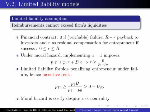
Limited liability assumption
Reimbursements cannot exceed firm’s liquidities
Financial contract: 0 if (verifiable) failure, R− r payback toinvestors and r as residual compensation for entrepreneur ifsuccess : 0 ≤ r ≤ RUnder moral hazard, implementing a = 1 imposes:
p1r ≥ p0r +B ⇐⇒ r ≥ Bp1−p0
Limited liability forbids penalizing entrepeneur under fail-ure, hence incentive rent:
p1r ≥p1B
p1 − p0> 0 = UR.
Moral hazard is costly despite risk-neutrality
Presentation: Francis Bloch, Slides: Bernard Caillaud Principal - Agent model under moral hazard

V.2. Limited liability models
Look for financial contracts that allow investors to breakeven (investors’ participation constraint):
I −W ≤ p1
(R− B
p1 − p0
)⇐⇒
W ≥ W ≡ p1B
p1 − p0− (p1R− I)
W ≥ incentive rent - project profitability
If incentive rent is larger than project profitability, thereexist a financial contract that implements a = 1 and allowsinvestors to break even only if enough self-financing
Optimal contract depends on relative bargaining power ofboth actors
Moral hazard implies credit market imperfection despite globalrisk neutrality
Presentation: Francis Bloch, Slides: Bernard Caillaud Principal - Agent model under moral hazard
V.2. Limited liability models
Applications of this simple model to many issues in coporatefinance: see textbook in corporate finance by Tirole.
Models with limited liability provides a trade-off between rentextraction and incentives, instead of insurance and incentives,but their predictions are very close to more standard models ofmoral hazard.
And they are much more tractable !
Presentation: Francis Bloch, Slides: Bernard Caillaud Principal - Agent model under moral hazard

Required readings
Chiappori, P.A., I. Macho, P. Rey and B. Salanie (1994),European Economic Review, Vol 38(8), 1527?1553
* Grossman, S. and O.Hart (1983), Econometrica, 51(1), 7-45
Hermalin, B. and M. Katz (1991), Econometrica, 59(6), 1735-1753
* Holmstrom, B (1979), Bell J. of Economics, 10, 74-91
Holmstrom, B. and P. Milgrom (1991), Journ. of Law, Eco-nomics and Organizations, Vol 7, 24-52.
* Laffont, J.-J. and D. Martimort (2002), The theory ofincentives: The Principal - Agent model, Princeton Univ.Press, Ch 4-5
MC - W - G, Ch 14 B.
Salanie, B. (2005), The Economics of Contracts: A Primer,2nd Edition, MIT Press, Part 5.
Presentation: Francis Bloch, Slides: Bernard Caillaud Principal - Agent model under moral hazard