Microeconomics 2 Lecture notes - Forsiden › studier › emner › sv › oekonomi › ECON... · 2 CHAPTER 1. MORAL HAZARD 1.1.1 E¢ciency versus Risk-Sharing Consider an interaction

Microeconomics 2

Lecture notes

Winter 2012

Notes from Lectures by P.Ray (TSE)

ii

Contents

1 Moral Hazard 11.1 Introduction . . . . . . . . . . . . . . . . . . . . . . . . . . . . 1

1.1.1 E¢ciency versus Risk-Sharing . . . . . . . . . . . . . . 21.1.2 E¢ciency versus Rent . . . . . . . . . . . . . . . . . . 4

1.2 The Role of Statistical Inference . . . . . . . . . . . . . . . . . 71.2.1 The Inference Problem . . . . . . . . . . . . . . . . . . 71.2.2 Full Inference . . . . . . . . . . . . . . . . . . . . . . . 81.2.3 Limited Inference . . . . . . . . . . . . . . . . . . . . . 101.2.4 Valuable Signals . . . . . . . . . . . . . . . . . . . . . . 11

1.3 Comments . . . . . . . . . . . . . . . . . . . . . . . . . . . . . 121.3.1 Simple Case . . . . . . . . . . . . . . . . . . . . . . . . 12

1.4 Applications . . . . . . . . . . . . . . . . . . . . . . . . . . . . 191.4.1 Partial Insurance . . . . . . . . . . . . . . . . . . . . . 191.4.2 E¢ciency Wage . . . . . . . . . . . . . . . . . . . . . . 211.4.3 Credit Markets . . . . . . . . . . . . . . . . . . . . . . 221.4.4 Group Lending . . . . . . . . . . . . . . . . . . . . . . 231.4.5 Moral Hazard in Teams . . . . . . . . . . . . . . . . . 241.4.6 Career Concerns . . . . . . . . . . . . . . . . . . . . . 25

2 References 27

iii

iv CONTENTS

Chapter 1

Moral Hazard

1.1 Introduction

Asymmetric information

1. Adverse selection: Mechanism designer seeks to have agents reportcertain information.

2. Moral hazard: Mechanism designer seeks to have agents take certainactions.

Examples

• salesman’s e§ort

• managers’s decision

These situations involve a trade-o§. In adverse selection, the trade o§ isbetween e¢ciency and cost (information rent). In moral hazard situations, wehave a similar trade-o§, this time between e¢ciency and the cost of incentivecompatibility. This cost takes two forms:

1. Risk-sharing, and

2. Rents.

We will look at two simple illustrations of these two costs.

1

2 CHAPTER 1. MORAL HAZARD

1.1.1 E¢ciency versus Risk-Sharing

Consider an interaction between two parties. The principal, a firm, seeks tomaximize q w, where q is the output and w is the wage; the price of theoutput is normalized to one. The agent, a worker, has utility u(w)e, wheree is the e§ort the agent exerts. We assume that the agent has a reservationlevel of utility u = u(w), where u0 > 0 > u00: u is concave, and thus the agentis risk-averse. The output can take one of two values:

q =

Q with probability p0 with probability 1 p

The agent can choose either to work with e§ort level e = E, in which casethe probability that the project is successful p is pE; or to shirk and exerte§ort e = 0, in which case the probability of success p is p0 < pE. We willassume that pEQ E p0Q, u, so that e = E is e¢cient.The timing of the interaction is as follows:

• First, the principal o§ers a contract to the agent.

• The agent then accepts or refuses the contract.

• If the agent refuses the contract he gets a reservation utility u. If thecontract is accepted, the agent then chooses the level of e§ort e 2{0, E}, which is unobservable by the principal.

• Finally, as a result of the agent’s choice, a quantity q is produced.

Complete Information

Under complete information in which all is observable, a contract can specifythe e§ort level e = E and a wage schedule of the form w if q = Q and w ifq = 0. The principal’s profit-maximization problem is

maxw,w

pEQ (pEw + (1 pE)w)

s.t. pEu(w) + (1 pE)u(w) E u (IR)

Since the agent is risk-averse (u00 < 0) whereas the principal is risk-neutral,the optimal contract is such that w = w (perfect insurance); the wage levelis then set so as to meet the agent’s participation constraint: and u(w) =u(w) = u + E. The condition pEQ E p0Q then ensures that thiscontract is better than inducing the agent to exert no e§ort (e = 0), whereaspEQ E u ensures that contracting is better than no contracting.

1.1. INTRODUCTION 3

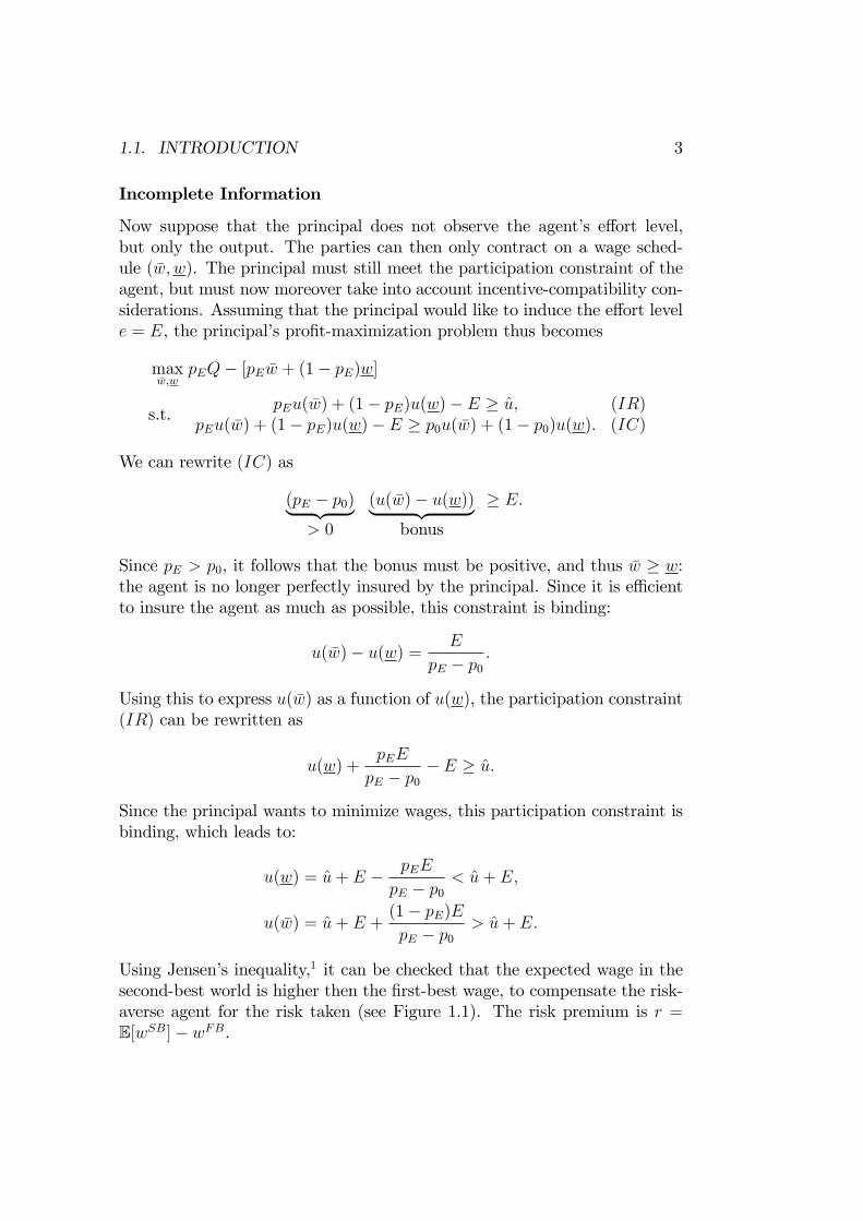
Incomplete Information

Now suppose that the principal does not observe the agent’s e§ort level,but only the output. The parties can then only contract on a wage sched-ule (w, w). The principal must still meet the participation constraint of theagent, but must now moreover take into account incentive-compatibility con-siderations. Assuming that the principal would like to induce the e§ort levele = E, the principal’s profit-maximization problem thus becomes

maxw,w

pEQ [pEw + (1 pE)w]

s.t.pEu(w) + (1 pE)u(w) E u, (IR)

pEu(w) + (1 pE)u(w) E p0u(w) + (1 p0)u(w). (IC)

We can rewrite (IC) as

(pE p0)| {z } (u(w) u(w))| {z }> 0 bonus

E.

Since pE > p0, it follows that the bonus must be positive, and thus w w:the agent is no longer perfectly insured by the principal. Since it is e¢cientto insure the agent as much as possible, this constraint is binding:

u(w) u(w) =E

pE p0.

Using this to express u(w) as a function of u(w), the participation constraint(IR) can be rewritten as

u(w) +pEE

pE p0 E u.

Since the principal wants to minimize wages, this participation constraint isbinding, which leads to:

u(w) = u+ E pEE

pE p0< u+ E,

u(w) = u+ E +(1 pE)EpE p0

> u+ E.

Using Jensen’s inequality,1 it can be checked that the expected wage in thesecond-best world is higher then the first-best wage, to compensate the risk-averse agent for the risk taken (see Figure 1.1). The risk premium is r =E[wSB] wFB.


u

u+ E

wwSB wSBE[wSB]wFB

Figure 1.1:

That e§ort provision is e¢cient in the first-best world does not guaranteethat it remains e¢cient in the second-best world; this also depends on thesize of the risk premium. Indeed, if:

pEQ E u > 0 > pEQ E u r,

then it is no longer optimal to induce the agent to exert e§ort; instead:

• If p0Qbu > 0, the second-best is to induce the agent to exert no e§ort:e = 0, w = w (distortion of the level of e§ort);

• If p0Q bu < 0, it is better not to contract (distortion of the level oftrade).

1.1.2 E¢ciency versus Rent

Assume now that the worker, too, is risk-neutral: u(w) = w, but has limitedliability:

w(q) w. (LL)

That is, the agent is always free to walk away from the job, should thecontracted wage fall below his reservation wage.

Complete Information

Under complete information, the parties can contract on the e§ort level (theprincipal will pay a non-zero wage only if e = E) and the output (w(q) = w

1For any concave function f (x), E [f (x)] f (E [x]).

1.1. INTRODUCTION 5

if the output q is low, and w(q) = w if the output q is high). The principal’sprofit-maximization problem is thus

maxw,w

pEQ [pEw + (1 pE)w]

s.t.pEw + (1 pE)w E w, (IR)

w, w w. (LL)

Ignoring (LL), the principal and the agent only care about the expectedwage we = pEw + (1 pE)w and, as the principal wants to minimize it,the participation constraint is binding and yields we = w + E. Conversely,setting w = w = w + E yields the desired expected wage and satisfies (LL);this is thus an optimal contract in this first-best. That is, limited liabilityhas no e§ect on the first-best solution.

Incomplete Information

Under incomplete information, the principal cannot observe the agent’s e§ortlevel and can only contract on a wage schedule (w, w). Assuming that theprincipal would like to induce the e§ort level e = E, the principal’s problembecomes:

maxw,w

pEQ [pEw + (1 pE)w]

s.t.pEw + (1 pE)w E w, (IR)

pEw + (1 pE)w E p0w + (1 p0)w, (IC)w, w w. (LL)

Using as variable the base wage w = w and the bonus b = w w, theparticipation constraint boils down to

w + pEb w + E,

whereas the incentive constraint can be rewritten as

w + pEb E w + p0b () b E

pE p0.

The bonus must therefore be positive, which in turn implies that, or the twolimited liability constraints (w,w+ b w), only the former one (for the basewage w) matters. The principal problem can thus be expressed as:

maxw,w

pEQ (w + pEb)

s.t.w + pEb w + E, (IR)

b EpEp0

, (IC)

w w. (LL)


maxw,w

pEQ [pEw + (1 pE)w]

Which of the three constraints are binding? If we ignore the participationconstraint (IR), the other two must be binding and determine the wageschedule: w = w from (LL) and b = E

pEp0from (IC); but then, the partici-

pation constraint is indeed satisfied:

w + pEb = w +pEE

pE p0= w + E +R > w + E,

where

R p0E

pE p0(1.1)

is the rent that the principal has to leave to the agent on top what is neededto accommodate the limited liability and incentive constraints. Thus, in thesecond-best world, the participation constraint is not an issue in presence oflimited liability: it is instead the limited liability constraint that binds.The cost of inducing the first-best level of e§ort is not just the cost of

e§ort E, but E + R; the principal must pay more than the cost of e§ort.Therefore, if:

pEQ E w > 0 > pEQ E w R,then:

• If p0Qw > 0, the second-best is to induce the agent to exert no e§ort:e = 0, w = w;

• If p0Q w < 0, it is better not to contract.

Variant

Consider the following variant of the above model:

• pE = 1 and p0 = 0: the project succeeds for sure if the agent choosesto work (e = E), and fails for sure otherwise (e = 0);

• there is no cost to e§ort, but instead the agent enjoys a private benefitB if he chooses to shirk.

In the first-best, e = E is e¢cient wheneverQ > B, in which case the firmo§ers a wage w = w for e = E. In the second-best, limited liability w w,and incentive compatibility requires ww B. At the (profit-maximizing)optimum, both constraints are binding and thus w = w + B (which in turnimplies that the participation constraint is satisfied: w > w). If

QB w < 0 < Q w,

it can be the case that e¢cient trade is not taking place.

1.2. THE ROLE OF STATISTICAL INFERENCE 7

1.2 The Role of Statistical Inference

The principal’s goal is to detect what the agent has done by observing relatedvariables, i.e. variables related to those that are relevant but not observable.In general, the principal will observe imperfect signals of the agent’s choice.

1.2.1 The Inference Problem

In the above examples, the principal seeks to infer the agent’s unobservede§ort e from the observed output q. Suppose more generally that there aren output levels q1 < q2 < . . . < qn, and the firm o§ers wages based on therealization of the output, w1 < w2 < . . . < wn. A natural question that arisesis, should the wage increase with the observed output level? The answer is,“Not necessarily”.To see this, consider the following example:

• the agent is risk-averse (but no limited liability)

• three output levels, q < q < q

• two levels of e§ort, e 2 {0, E}

• the probability distribution of the various outputs, given the agent’se§ort level, is as follows:

p q q qe = 0 9/10 1/10 0e = E 1/10 0 9/10

Assuming that the principal wants to induce the agent to exert e§ort(e = R), what is the second-best optimal wage schedule, w (q) = (w, , w, w)?In the absence of limited liability constraints it is optimal to punish the agent“infinitely” if q is observed: w = 1, as observing q would reveal that theagent shirked. This, in turn, would su¢ce to provide the e§ort incentives,and thus full insurance is possible: w = w, where the wage level is set so asto meet the agent’s participation constraint: u(w) = u(w) = u + E. Thus,the optimal wage schedule is not monotonic, but instead goes down steeplywhen the output increases from q to q, before increasing as steeply when theoutput increases from q to q.


1.2.2 Full Inference

Suppose that the output level is given by q = q(e)+", where q(·) is one-to-oneand where the noise " is distributed over the support [,] according tothe c.d.f F (·). The e§ort level chosen by the agent thus a§ects the support.Thus, whenever the agent deviates from a prescribed e§ort level, there is apositive probability that the deviation will be detected. For example, if theagent is asked to choose eFB, and chooses instead e < eFB, then the supportof the output moves from

eFB , eFB +

to [e, e+], and thus the

deviation is detected whenever q 2 [e, eFB ), or " 2, eFB e

,

that is, it is detected with probability FeFB e

. It follows that the first-

best is implementable at no additional cost if you can su¢ciently punish theagent.Mirrlees (1975, RES 1999) shows that the argument extends to some

situations where deviations are never detected for sure. Suppose for examplethat " F (·) over R, where F (") ! 0 as " ! 1, and F (")/f(") ! 0 as" ! 1. (This last condition simply says that the cdf F (·) goes to zerofaster than the density f(·) does; it is satisfied for example by the normaldistribution.)In a first-best world, the principal’s profit-maximization problem is

maxe,w(q)

E[q w(q)|e]

s.t. E[u(w(q)) e|e] u

Assuming that the agent’s utility function is increasing and concave with thewage (u0 > 0 > u00), it is then optimal for the principal to provide full insur-ance and to set the wage so as to meet the agent’s participation constraint:w(q) = w = h (e) u1(u + e). The principal’s objective function thusbecomes (using E [q] = E [e+ "] = e)

maxee h(e),

where u” < 0 < u0 implies h0, h00 > 0. This objective function is thusconcave, and the first-order condition yields the first-best level of e§ort eFB:h0(eFB) = 1.Consider now the second-best setting, and the following schedule (it is

more convenient to express it in terms of the agent’s utility, u (w), ratherthan in terms of the wage w):

u =

U if q Q,

U P if q < Q.


The parameters of the compensation scheme are U , P and Q: the agent isguaranteed a fixed utility U as long as he “delivers” an output at least equalto Q, and incurs a penalty P otherwise.Failing to meet the threshold Q amounts to

q = e+ " Q() " Q e,

and thus happens with probability F (Q e). The agent’s expected utility istherefore given by

F (Q e)(U P ) + (1 F (Q e))U e = U F (Q e)P e.

To induce the agent to choose the first-best level of e§ort, it then su¢ces toset P so as to satisfy the first-order condition

f(Q eFB)P = 1() P =1

f(Q eFB). (1.2)

The individual-rationality condition,

U F (Q eFB)P eFB u,

leading the principal, for any given Q, to set U to:

U = u+ eFB +F (Q eFB)f(Q eFB)

.

By assumption, F (Q eFB)/f(Q eFB) ! 0 as Q ! 1. Therefore,asymptotically, reducing the threshold Q to 1 (and increasing the penaltyP to 1, so as to maintain incentives) allows the principal to implement thefirst-best outcome at no additional cost.Limitations of this approach:

• We needed to make an assumption on the distribution.

• In practice, there is a de facto upper bound on the penalty we canimpose on the agents, due to limited liability. That is, in real life,agents will not be able to pay a fine of, say, 500 million euros.

• The penalty is chosen relying on the fact that you know exactly theprobability of very unlikely events (about the tail of the distribution).


1.2.3 Limited Inference

We just saw several examples in which the inference problem could be fullysolved, in which case moral hazard has no bite: incentive constraints arecostless. In the remainder of this chapter, we will focus on situations oflimited inference, in which incentive constraints come at a cost.Suppose for example that the output level q is distributed over the support

[0, Q], and that the agent can choose between two di§erent levels of e§ort,0 and E > 0, giving rise to density functions f0(q) and fE(q), respectively.Assume that the agent has an outside option that yields utility u. We assumethat the following condition holds:Assumption (Monotone Likelihood Ratio Property — MLRP):

The likelihood ratio

l(q) =fE(q) f0(q)

fE(q)

is increasing in q.The principal wants to induce the high level of e§ort in the agent, i.e. e =

E; she must therefore choose a wage schedule w(q) that satisfies individualrationality and incentive compatibility. The principal’s profit-maximizationproblem can thus be stated as:

maxw(·)

Z Q

0

(q w(q)) fE(q) dq

s.t.R Q0u (w(q)) fE(q) dq E u, (IR)R Q

0u (w(q)) fE(q) E

R Q0u(w(q))f0(q) dq. (IC)

Denote the multipliers for these constraints by and µ respectively; theLagrangian of this problem is

L =

Z Q

0

[q w(q) + u(w(q)) (u+ E)

+ µu(w(q))fE(q) f0(q)

fE(q) µE]fE(q) dq.

Note that , µ 0. The first-order condition with respect to w(q), for agiven q, yields

(+ µl(q)) u0(w(q)) = 1, (1.3)

where l(q) is the likelihood ratio defined above. Since l(q) is increasing in q,the first term + µl(q) is increasing in q. Under the assumption of concaveutility, the second term u0(w(q)) is decreasing in w(q). So as q increases,w(q) increases.


Note: The reasoning relies on µ > 0, which indeed holds at the optimum.To see this, note that if µ = 0, then the first-order condition (1.3) reducesto u0(w(q)) = 1. This would imply full insurance (w(q) = w), but then aconstant wage does not satisfy the incentive constraint (IC), a contradiction.Hence we must have µ > 0.

1.2.4 Valuable Signals

Intuitively, have more informative signals facilitate inference and thus reducesthe cost of providing incentives.

Example

Consider the following example:

• the agent is risk-neutral but has limited liability;

• the agent can choose among two levels of e§ort: e 2 {0, E};

• the output is either 0 or Q;

• the principal observes the output and another signal which can taketwo values, 0 and E, with probabilities given by the following table:

E§ort e Output q Signal

0 q =

Q with probability p00 with probability 1 p0

=

E with probability 00 with probability 1 0

E q =

Q with probability pE0 with probability 1 pE

=

E with probability E0 with probability 1 E

We will assume further that E > 0, so that “right” signal E is morelikely when the agent exerts e§ort.

If the principal chooses to ignore the signal when designing the contract,then we are back to the example studied above, in which she o§ers the agent abase wage w = w and a bonus b designed to meet the incentive-compatibilitycondition:

b =E

pE p0,

which leaves a rent to the agent, equal to

r = pEb E =p0E

pE p0.


Suppose now that the principal includes the signal in the contract design,and o§ers the agent a base wage w, with a bonus B only if she observesboth the high-level output Q and the “right” signal E. The incentive-compatibility condition is then

w + EpEB E w + 0p0B,

which we can rearrange as

(EpE 0p0)B E.

The minimum bonus b satisfying incentive compatibility in this contract isthus

B =E

EpE 0p0,

and the minimum informational rent the principal would need to give is

R = EpEB E =EpEE

EpE 0p0 E

=0p0E

EpE 0p0

=p0E

E0pE p0

< r =p0E

pE p0,

where the last inequality stems from the assumption that E > 0 (if E < 0,it su¢ces to swap the roles of E and 0; thus, what matters if the signalis “informative”, in the sense that E 6= 0). This rent is therefore strictlyless than the rent paid in the contract when the principal ignored the signal;that is, the signal is indeed valuable to the principal.Holmstrom (Bell 1979) developed the idea and showed that the principal

should base the contract on a su¢cient statistic of the signals available. Thatis, any informative signal should be included in the contract. But if one ofthe signals is perfectly colinear with a linear combination of the other signals,then it need not be included in the contract.

1.3 Comments

1.3.1 Simple Case

Assume limited liability and risk neutrality. There are two possible outcomes,0 or Q. The agent can choose any e§ort e 2 R+, in which case the probability

1.3. COMMENTS 13

of realizing the high output is p(e), where p (0) = 0 and p0 > 0 > p00, and thecost to the agent is c(e), where c (0) = 0 and c0, c00 > 0.In a complete-information setting, the agent seeks to maximize

maxep(e)Q c(e),

which is concave in e; the first-best level of e§ort eFB thus solves the first-order condition:

p0(e)Q = c0(e).

In a second-best world, principal seeks to o§er the bonus b that maximizes

maxep(e)b c(e).

Define e(b) to be the solution to this maximization problem. By a revealedpreference argument, b(e) is increasing: for any b and b0, letting e = e (b)ande0 = e (b0) denote the corresponding e§ort levels, we have: pb c p0b c0

and p0b0 c0 pb0 c, which implies: (p p0)(b b0) 0. The function e (b)can therefore be inverted; let b (e) denote the bonus needed to induce a givenlevel of e§ort e. The agent’s objective is strictly concave under our convexityconditions, and thus b (e) is given by the first-order condition:

p0(e)b = c0(e), b(e) =c0(e)

p0(e).

This bonus satisfies b (0) = 0 (maximizing p (e) bc (e) = c (e) indeed leadsthe agent to exert no e§ort, e = 0) and increases in e. The cost of inducingthe e§ort level e is then

p(e)b(e) = c(e) + r (e) ,

where the rentr(e) p(e)b(e) c(e)

is such that r (0) = 0 and, using the envelope theorem:

r0(e) = p(e)b0(e) > 0.

This implies that, the rent r (e) is positive for any e > 0; it also implies thatthe second-best e§ort level eSB, maximizing the principal net payo§

maxep(e)Q c(e) r(e),

satisfiesp0(e)Q = c0(e) + r0 (e) > c0 (e)

and is thus strictly lower than the first-best


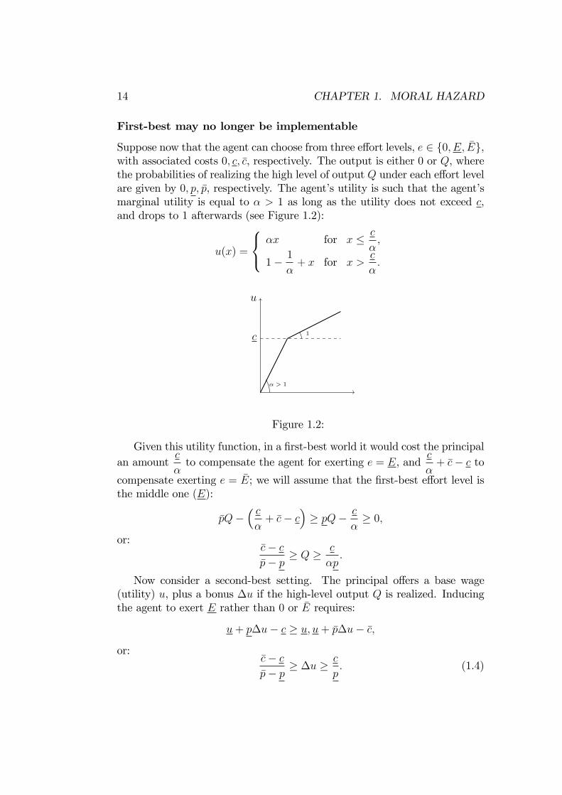
First-best may no longer be implementable

20Suppose now that the agent can choose from three e§ort levels, e 2 {0, E, E},with associated costs 0, c, c, respectively. The output is either 0 or Q, wherethe probabilities of realizing the high level of output Q under each e§ort levelare given by 0, p, p, respectively. The agent’s utility is such that the agent’smarginal utility is equal to > 1 as long as the utility does not exceed c,and drops to 1 afterwards (see Figure 1.2):

u(x) =

8<

:x for x

c

,

11

+ x for x >

c

.

u

c

> 1

1

Figure 1.2:

Given this utility function, in a first-best world it would cost the principalan amount

c

to compensate the agent for exerting e = E, and

c

+ c c to

compensate exerting e = E; we will assume that the first-best e§ort level isthe middle one (E):

pQ c+ c c

pQ

c

0,

or:c cp p

Q c

p.

Now consider a second-best setting. The principal o§ers a base wage(utility) u, plus a bonus u if the high-level output Q is realized. Inducingthe agent to exert E rather than 0 or E requires:

u+ pu c u, u+ pu c,

or:c cp p

u c

p. (1.4)

1.3. COMMENTS 15

Therefore, if:c

pc cp p

Q c

p,

then:

• the first-best e§ort level is E;

• and yet inducing this first-best e§ort level is infeasible in a second-bestsetting, since the this range characterized by (1.4) is empty (since thelower bound, cc

pp , exceeds the upper one,cp).

The participation constraint may not be binding

This is clearly the case when the agent is subject to limited liability, as thesimple example studied in the introduction shows: incentive-compatibilityand limited liability may then be the only relevant constraints in that case,and require the principal to leave a rent to the agent, in addition to whatwould be needed to meet the agent’s participation constraint.When the agent is not subject to limited liability but is risk-averse, wealth

e§ects may play a role, in such a way that participation may not be binding.That is, if the agent’s utility is of the form u(w, e), increasing the e§ort emay a§ect the agent’s risk aversion, and increasing the wealth w may alsolower the agent’s disutility of e§ort. In addition, merely replacing the agent’sincentive constraint by the associated first-order condition is not necessarilyvalid; as shown by Mirrlees (1975, RES 1999), the corresponding first-ordercondition of the principal’s optimization problem may then be neither nec-essary nor su¢cient. To avoid these issues, Grossman & Hart (Econometrica1983) consider utility functions that are (additively and/or multiplicatively)separable in w and e, in which case they are able to develop an alternativeapproach that does not rely on the agent’s first-order condition, and whichconsists in first characterizing the cost of inducing a particular e§ort level(implementation stage), before studying the optimal choice of e§ort (opti-mization stage).Note: We can also interpret limited liability as an extreme form of risk-

aversion; for example, a utility of the form U = u (w) c (e), where (seeFigure 1.3):

u(w) =

w for w w1 for w < w

,

leads to an analysis that is formally identical to the case of a risk-neutralagent facing a limited liability w w.


u

w

Figure 1.3:

Multi-tasking

Let there be two tasks to be assigned to either one or two agents, both withlimited liability (w w). For each task:

• the agent in charge can choose from two levels of e§ort, e 2 {0, E};

• the output level is also binary, q 2 {0, Q}, with independent probabil-ities of success;

• the probability of realizing the high output Q given by p0 > 0 if theagent chooses e = 0 and by pE > p0 if the agent chooses e = E.

If an agent is assigned a single task, then from the analysis of 1.1.2 (see(1.1)), the principal must give the agent a rent

R1 =p0E

pE p0.

Thus, if the principal assigns the two tasks to di§erent agents, the totalinformation rent he will have to pay is 2R1.The principal can however do better by giving both tasks to the same

agent; in that case, instead of rewarding “in cash” the agent for the successof one task, the principal can grant the agent a stake (i.e., a fraction of theoutput produced) in the other task, which contributes to foster the agent’sincentive to behave in the management of that other task. To see this,suppose that the principal gives a bonus B to the agent only if both projectssucceed. To induce the agent to exert e§ort in both projects, the principalneeds to ensure that the agent’s expected payo§ when the agent chooses(e1, e2) = (E,E) is weakly greater than his expected payo§ when (i) he

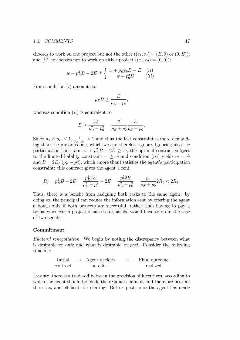
1.3. COMMENTS 17

chooses to work on one project but not the other ((e1, e2) = (E, 0) or (0, E));and (ii) he chooses not to work on either project ((e1, e2) = (0, 0)):

w + p2EB 2E w + pEp0B E (ii)

w + p20B (iii)

From condition (i) amounts to

pEB E

pE p0,

whereas condition (ii) is equivalent to

B 2E

p2E p20=

2

pE + p0

E

pE p0.

Since p0 < pE 1, 2pE+p0

> 1 and thus the last constraint is more demand-ing than the previous one, which we can therefore ignore. Ignoring also theparticipation constraint w + p2EB 2E w, the optimal contract subjectto the limited liability constraint w w and condition (iii) yields w = wand B = 2E/ (p2E p20), which (more than) satisfies the agent’s participationconstraint: this contract gives the agent a rent

R2 = p2EB 2E =

p2E2E

p2E p20 2E =

p202E

p2E p20=

p0pE + p0

2R1 < 2R1.

Thus, there is a benefit from assigning both tasks to the same agent: bydoing so, the principal can reduce the information rent by o§ering the agenta bonus only if both projects are successful, rather than having to pay abonus whenever a project is successful, as she would have to do in the caseof two agents.

Commitment

Bilateral renegotiation. We begin by noting the discrepancy between whatis desirable ex ante and what is desirable ex post. Consider the followingtimeline:

Initial ! Agent decides ! Final outcomecontract on e§ort realized

Ex ante, there is a trade-o§ between the provision of incentives, according towhich the agent should be made the residual claimant and therefore bear allthe risks, and e¢cient risk-sharing. But ex post, once the agent has made


his decision, incentives are no longer an issue and the parties would thereforebenefit from sharing the risk in an e¢cient way. Thus, once the e§ort decisionis made, the principal and agent have an incentive to renegotiate the originalcontract in order to optimize risk-sharing. But then, anticipating that he willbe fully insured, the agent will no longer has an incentive to exert any e§ort.That is, while ex post the parties can benefit from renegotiating the originalcontract, anticipating this renegotiation will backfire: the agent will not basehis e§ort decision on the initial contract, but rather on the anticipated finalcontract.

In the same vein, in a multi-period setting the principal would ideallywish to contract on the agent’s consumption plan. However, in practice, theparties contract on the agent’s compensation, and the agent remains free toborrow or save. Thus, the contract should not only provide incentives withrespect to the choice of e§ort, but also with respect to savings; in particular,Rogerson (Econometrica 1985) shows that, the contract that would be opti-mal if the parties could directly contract on the agent’s savings is such that,if the agent would like to save more if he could do so secretly. However, inlater periods, there is no reason anymore to account for the agent’s incen-tives about past savings decisions, and thus the parties would benefit fromreplacing the (continuation of) the original contract with another one that ismore e¢cient for the remaining periods.

One way to alleviate this problem is to make it unclear whether the agenthas actually chosen the e§ort before the renegotiation (that is, induce theagent to randomize). See e.g., Fudenberg & Tirole (Econometrica 1990) andMa (QJE 1991) for within-period contracting, and Chiappori et al. (EER1994) for multi-period contracting.

Unilateral renegotiation. The above analysis also relies on the assumptionthat the principal can commit to pay performance-based bonuses; however,ex post, the principal may be tempted to claim that performance was poor,even if it was actually good, in order to avoid paying the bonus. Commitmentmay thus not be credible if the agent’s performance is not readily observedby third parties such as judges or courts. One way consists in introducingtournaments and prize systems; the principal can then commit herself to givea prize to someone, and has no reason not to give it the best performer.

1.4. APPLICATIONS 19

1.4 Applications

1.4.1 Partial Insurance

Consider the example of car insurance. The agent is a driver, with wealth wand utility u(w). With probability 0 there is no accident; with probabilityi there is an accident generating a loss Li, where i = 1, . . . , n. The principalis an insurance company, o§ering a policy that involves a fee and reimbursesthe driver an amount i (on top the fee ) in the case of an accident withloss Li.The insurance company’s expected profit is

V = 0 X

i>0

i (c+ (1 + )i) ,

where c denotes a fixed transaction cost per accident, and denotes anadditional transaction cost that varies proportionally with the amount atstake, i. The insurance company seeks to maximize its expected profit,subject to the driver’s participation constraint:

U = 0u(w ) +nX

i=1

iu(w Li + i) U = 0u(w) +nX

i=1

iu(w Li).

Let 0 denote the Lagrangian multiplier of the participation constraint.In a first-best world, this constraint is necessarily binding (since the principalwishes for example to maximize the fee ) and thus > 0; the correspondingfirst-order conditions are

w.r.t. : 0 0u0(w ) = 0,w.r.t. i : i(1 + ) + iu0(w Li + i) = 0,

which we can simplify to

w.r.t. : w = u011

,

w.r.t. i :w Li + i = u011 +

.

It follows that, for i = 1, . . . , n, the driver’s net wealth w Li + i remainsconstant and equal to u01 ((1 + )/). That is, conditional on having anaccident, the driver ends up with the same net wealth: the driver is thusfully insured against the gravity of the accident. Furthermore, if = 0,then w Li + i = w (= u01 (1/)): we have full insurance. If instead


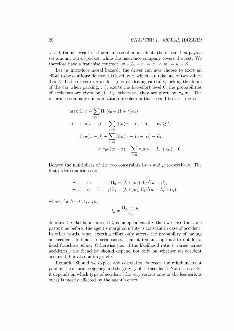
> 0, the net wealth is lower in case of an accident: the driver then pays aset amount out-of-pocket, while the insurance company covers the rest. Wetherefore have a franchise contract: w Li + i = w < w+ = w .Let us introduce moral hazard: the driver can now choose to exert an

e§ort to be cautious; denote this level by e, which can take one of two values0 or E. If the driver exerts e§ort (e = E: driving carefully, locking the doorsof the car when parking, ...), exerts the low-e§ort level 0, the probabilitiesof accidents are given by 0,i; otherwise, they are given by 0, i. Theinsurance company’s maximization problem in this second-best setting is

max 0 X

i>0

i (c0 + (1 + )i)

s.t. 0u(w ) +X

i>0

iu(w Li + i) Ei U

0u(w ) +X

i>0

iu(w Li + i) Ei

0u(w ) +X

i>0

iu(w Li + i) 0.

Denote the multipliers of the two constraints by and µ respectively. Thefirst-order conditions are

w.r.t. : 0 = (+ µl0)0u0(w ),

w.r.t. i : (1 + )i = (+ µli)iu0(w Li + i),

where, for h = 0, 1, ..., n,

lh =h hh

denotes the likelihood ratio. If li is independent of i, then we have the samepattern as before: the agent’s marginal utility is constant in case of accident.In other words, when exerting e§ort only a§ects the probability of havingan accident, but not its seriousness, than it remains optimal to opt for afixed franchise policy. Otherwise (i.e., if the likelihood ratio li varies acrossaccidents), the franchise should depend not only on whether an accidentoccurred, but also on its gravity.Remark: Should we expect any correlation between the reimbursement

paid by the insurance agency and the gravity of the accident? Not necessarily;it depends on which type of accident (the very serious ones or the less seriousones) is mostly a§ected by the agent’s e§ort.


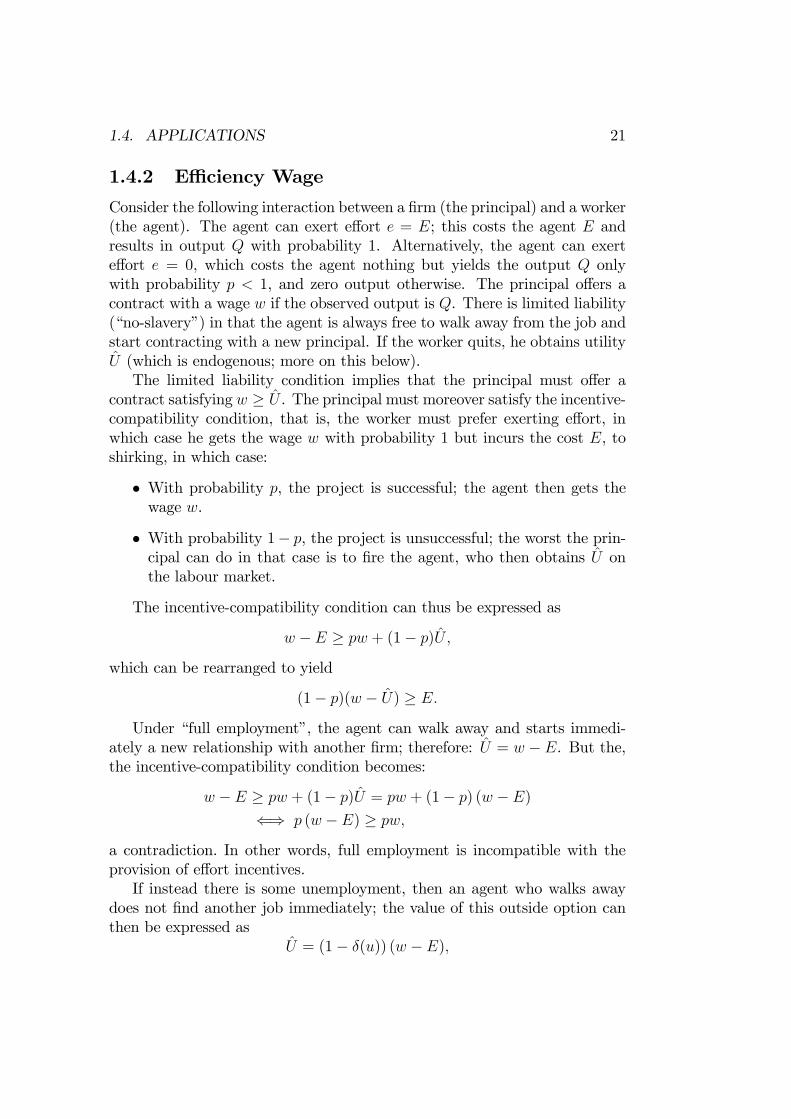
1.4.2 E¢ciency Wage

Consider the following interaction between a firm (the principal) and a worker(the agent). The agent can exert e§ort e = E; this costs the agent E andresults in output Q with probability 1. Alternatively, the agent can exerte§ort e = 0, which costs the agent nothing but yields the output Q onlywith probability p < 1, and zero output otherwise. The principal o§ers acontract with a wage w if the observed output is Q. There is limited liability(“no-slavery”) in that the agent is always free to walk away from the job andstart contracting with a new principal. If the worker quits, he obtains utilityU (which is endogenous; more on this below).The limited liability condition implies that the principal must o§er a

contract satisfying w U . The principal must moreover satisfy the incentive-compatibility condition, that is, the worker must prefer exerting e§ort, inwhich case he gets the wage w with probability 1 but incurs the cost E, toshirking, in which case:

• With probability p, the project is successful; the agent then gets thewage w.

• With probability 1 p, the project is unsuccessful; the worst the prin-cipal can do in that case is to fire the agent, who then obtains U onthe labour market.

The incentive-compatibility condition can thus be expressed as

w E pw + (1 p)U ,

which can be rearranged to yield

(1 p)(w U) E.

Under “full employment”, the agent can walk away and starts immedi-ately a new relationship with another firm; therefore: U = w E. But the,the incentive-compatibility condition becomes:

w E pw + (1 p)U = pw + (1 p) (w E)() p (w E) pw,

a contradiction. In other words, full employment is incompatible with theprovision of e§ort incentives.If instead there is some unemployment, then an agent who walks away

does not find another job immediately; the value of this outside option canthen be expressed as

U = (1 (u)) (w E),


where u denotes the unemployment rate, and the discount rate increaseswith unemployment. Each firm, maximizing its expected profit subject to theabove incentive constraint, will make this constraint binding; in equilibrium,we thus have:

w E = pw + (1 p)U = pw + (1 p) (1 (u)) (w E),

or

w = w (u) E +pE

(1 p)(u).

Notice that the equilibrium wage w decreases as the rate of unemploymentu increases. For further analysis, see Shapiro & Stiglitz (AER 1984).

1.4.3 Credit Markets

Consider a firm with an initial asset A which has a project costing I > A; tofinance the project, the firm must therefore seek external investors. The firmmanager (the agent) can either “behave”, in which case the project producesoutput Q with probability 1; or he can “shirk”, in which case the projectproduces no output Q but the manager then enjoys a private benefit B. Itis e¢cient to finance the project when the manager behave if

Q > I.

The project is e¢cient, and Let R denote the amount the firmmust reimbursethe lender. The incentive-compatibility constraint in this problem is

QR B,

or:R R QB,

where R represents the pledgeable income, that is, the maximal amount thatthe firm can credibly repay — any higher amount R > R would violate theincentive-compatibility, implying that the firm manager will choose to shirk— and thus no repayment would ever be made.Note that this pledgeable income is negative when B > Q, that is, when

shirking would actually be e¢cient; in that case, while it would still bee¢cient to undertake the project if B > I, it cannot be financed. Even ifQ > B, so that inducing the manager to behave is more e¢cient, the most afirm can raise via external financing is

I A R,


orA A I R = I (QB),

where A > 0 as long as Q < B + I. In that case, it is only the firms withinitial assets at least as large as A who get financed — in other words, "therich get richer".

1.4.4 Group Lending

Consider a variant of the above model in which “shirking” still produces theoutput Q with some probability p < 1 (and no output otherwise). Goingthrough the same steps as above, the pledgeable incomes becomes

R1 QB

1 p,

and the associated threshold level for the initial assets becomes

A1 I R1 = I (QB

1 p).

In what follows, we will suppose that this threshold is positiveA1 > 0

, so

that an entrepreneur with initial assets A < A1 cannot finance his project.Suppose now that:

• there are n such entrepreneurs, each with a project similar as the firstone (and independent realizations, in case of shirking);

• each entrepreneur’s initial asset is lower than A1, which prevents theentrepreneur from seeking investors on an individual basis.

We now show that, by grouping their projects, the entrepreneurs may beable to secure financing, provided they can coordinate their e§ort decisions.To see this, suppose first that their regroup their projects, so that the

reimbursement for one project may now depend on the outcomes of all theprojects, but keep choosing their e§orts independently from each other.An entrepreneur’s individual incentive-compatibility constraint becomes

Q E[R] p(Q E[R]) +B,

where E [R] denotes the expected reimbursement, given the distribution of theoutcomes of the other projects. But then, E [R] cannot exceed R1, which inturn implies that the entrepreneur would need at least A1 to secure financing.


Suppose now that the n entrepreneurs take their e§ort decisions jointly,so as to maximize their joint payo§. Building on the insights from section1.3.1 on multi-tasking, the best contract then consist in leaving the entrepre-neurs a return only if all projects are successful — that is, successful projectsshould pay back the loan to unsuccessful ones. The contract must inducethe entrepreneurs to behave rather than to shirk on any k n projects;therefore, the following incentive-compatibility conditions must be satisfiedfor k = 1, ..., n:

n (QR) npk(QR) + kB,

or

QR kB

n (1 pk).

It can be checked that the right-hand side of RHS this condition increases ink:

d

dk

kB

n (1 pk)

=B1 pk + k (log p) pk

n (1 pk)2,

and thus has the same sign as f (x) = 1 x+ x log x, where x = pk 2 [0, 1].Since f 0 (x) = log x < 0 on this range, f (x) f (1) = 0.Therefore, the most demanding constraint is the one for k = n, which

amounts to

R Rk QB

1 pn,

which in turn leads to

A Ak I (QB

1 pn),

where the threshold level Ak decreases as n increases. It is thus easier tofinance the projects by regrouping them.

1.4.5 Moral Hazard in Teams

Consider a team of two agents, where the output Q produced by the team isequal to the sum of the agents’ contributions: Q = e1+ e2. Assume that thecost of e§ort to Agent i is given by ci(ei), where c0i, c

00i 0 for i = 1, 2.

In a first-best world, the agents solve

maxe1,e2

e1 + e2 (c1(e1) + c2(e2)) .

This program is concave, and the solution eFBi thus satisfies c0i(eFBi ) = 1 for

all i.


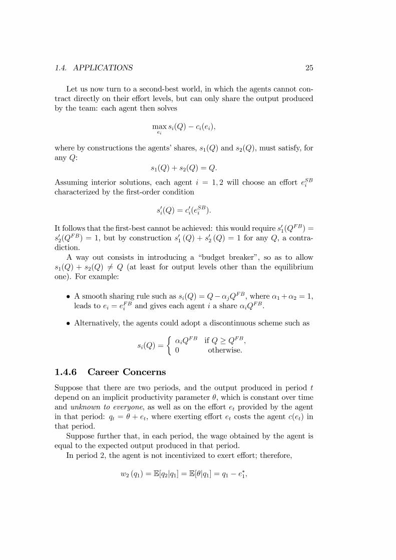
Let us now turn to a second-best world, in which the agents cannot con-tract directly on their e§ort levels, but can only share the output producedby the team: each agent then solves

maxeisi(Q) ci(ei),

where by constructions the agents’ shares, s1(Q) and s2(Q), must satisfy, forany Q:

s1(Q) + s2(Q) = Q.

Assuming interior solutions, each agent i = 1, 2 will choose an e§ort eSBicharacterized by the first-order condition

s0i(Q) = c0i(e

SBi ).

It follows that the first-best cannot be achieved: this would require s01(QFB) =

s02(QFB) = 1, but by construction s01 (Q) + s

02 (Q) = 1 for any Q, a contra-

diction.A way out consists in introducing a “budget breaker”, so as to allow

s1(Q) + s2(Q) 6= Q (at least for output levels other than the equilibriumone). For example:

• A smooth sharing rule such as si(Q) = QjQFB, where 1+2 = 1,leads to ei = eFBi and gives each agent i a share iQFB.

• Alternatively, the agents could adopt a discontinuous scheme such as

si(Q) =

iQ

FB if Q QFB,0 otherwise.

1.4.6 Career Concerns

Suppose that there are two periods, and the output produced in period tdepend on an implicit productivity parameter , which is constant over timeand unknown to everyone, as well as on the e§ort et provided by the agentin that period: qt = + et, where exerting e§ort et costs the agent c(et) inthat period.Suppose further that, in each period, the wage obtained by the agent is

equal to the expected output produced in that period.In period 2, the agent is not incentivized to exert e§ort; therefore,

w2 (q1) = E[q2|q1] = E[|q1] = q1 e1,


where e1 denotes the e§ort expected from the agent in period 1. It followsthat, in period 1, the agent will seek to maxzimize

maxe1E[w1 c(e1) + w2 (q1) = w1 c(e1) + ( + e1 e1) ,

where denotes the discount factor attached to period 2. This leads toe1 = e

1, characterized by:

c0(e1) = .

It follows that the agent will exert too much e§ort when > 1 (that is, atthe beginning of the career, interpreting “period 2” as representing all thefuture periods of activity), and will instead exert too little e§ort when < 1(towards the end of the career).More generally, learning about the agent’s productivity is more progres-

sive (the output also depends on a noise "t, say), and this productivity maynot be constant over time. See e.g. Dewatripont, Jewitt and Tirole (RES1999) for more discussion.

Chapter 2

References

Akerlof, G. (1970), “The market for Lemons: Quality uncertainty and themarket mechanism,” Quarterly Journal of Economics, 89:488-500.Attar, A., Th. Mariotti and F. Salanié (2011), “Nonexclusive Competi-

tion in the Market for Lemons,” Econometrica, 79(6):1869-1918.Baron, D., and R. Myerson (1982), “Regulating a Monopolist with Un-

known Costs”, Econometrica, 50:911-930.Bester, H., and R. Strausz (2001), “Contracting with Imperfect Commit-

ment and the Revelation Principle: The Single Agent Case,” Econometrica,69(4):1077-98.Bolton, P. and M. Dewatripont (2005), Contract Theory, MIT Press.Chiappori, P.-A., I. Macho, P. Rey and B. Salanié (1994), “Repeated

Moral Hazard: The Role of Memory, Commitment, and the Access to CreditMarkets,” European Economic Review, 38(8):1227-1253.Clarke, E. H. (1971), “Multipart pricing of public goods,” Public Choice,

17-33.Dasgupta, P., P. Hammond and E. Maskin (1979), “The Implementation

of Social Choice Rules: Some General Results on Incentive Compatibility”,Review of Economic Studies, 46:185-216.D’Aspremont, C., and L.A. Gérard-Varet (1979), “Incentives and Incom-

plete Information”, Journal of Public Economics, 11:24-45.Dewatripont, M., I. Jewitt and J. Tirole (1999), “The Economics of Ca-

reer Concerns, I: Comparing Information Structure,” The Review of Eco-nomic Studies, 66(1):183-198.Fudenberg, D., and J. Tirole (1990), “Moral Hazard and Renegotiation

in Agency Contracts,” Econometrica, 58(6):1279-1319.Fudenberg, D., and J. Tirole (1991), Game Theory, MIT Press, Cam-

bridge.

27

28 CHAPTER 2. REFERENCES

Gibbard, A. (1973), “Manipulation of Voting Schemes: A General Re-sult”, Econometrica, 41:587-601.Gibbons, R. (1992), A Primer in Game Theory, Harvester Wheatsheaf,

N.Y.Green, J., and J.J. La§ont (1979), Incentives in Public Decision Making,

North Holland: Amsterdam.Grossman, S., and O. Hart (1983), “An Analysis of the Principal-Agent

Problem”, Econometrica, 51:7-45.Groves, T. (1973), “Incentives in Teams”, Econometrica, 41:617-631.Guesnerie, G., and J.-J. La§ont (1984), “A Complete Solution of Principal-

Agent Problems with an Application to the Control of a Self-Managed Firm”,Journal of Public Economics, 25:329-369.Holmstrom, B. (1979), “Moral Hazard and Observability”, Bell Journal

of Economics, 10:74-91.Hirshleifer, J. (1971), “The Private and Social Value of Information and

the Reward to Inventive Activity,” American Economic Review, 61:561-574.La§ont, J.J. (1988), Fundamentals of Public Economics, MIT Press, Cam-

bridge.La§ont, J.J. (1986), The Economics of Uncertainty and Information,

MIT Press, Cambrigde. Version française: Economie de l’Incertain et del’Information, Economica, Paris.La§ont, J.J. and D. Martimort (2002), The Theory of Incentives: The

Principal Agent Model, Princeton University Press.La§ont, J.J., and E. Maskin (1979), “A Di§erentiable Approach to Ex-

pected Utility Maximizing Mechanisms”, Chap. 16 in La§ont, J.J. ed., Ag-gregation and Revelation of Preferences, North-Holland: Amsterdam.La§ont, J.J., and E. Maskin (1980), “A Di§erential Approach to Domi-

nant Strategy Mechanisms”, Econometrica, 48:1507-1520.La§ont, J.J., and E. Maskin (1982), “The Theory of Incentives: An

Overview”, in W. Hildenbrand (ed.), Advances in Economic Theory, Cam-bridge University Press.La§ont, J.J., and J. Tirole (1986), “Using Cost Observation to Regulate

Firms”, Journal of Political Economy, 94(3):614-641Leininger, W., P. B. Linhart and R. Radner (1989), “Equilibria of the

sealed-bid mechanism for bargaining with incomplete information”, Journalof Economic Theory, 48(1):63-106.Ma, A. (1991), “Adverse Selection in Dynamic Moral Hazard,” Quarterly

Journal of Economics, 106:255-275.Mas-Colell, A., M.D. Whinston and J. Green (1995),Microeconomic The-

ory, Oxford University Press, New York and Oxford.

29

Maskin, E. (1985), “The Theory of Implementation in Nash Equilibrium:A Survey”, Social Goals and Social Organization, Essays in memory of ElishaPazner, L. Hurwicz, D. Schmeidler and H. Sonnenschein eds., CambridgeUniversity Press.Maskin, E. (1999), “Nash Equilibrium and Welfare Optimality”, Review

of Economic Studies, 66:23-38.Mirrlees, J. (1975), “The Theory of Moral Hazard and Unobservable Be-

haviour: Part I”, reprinted in Review of Economic Studies, 66(1):3—21, Jan-uary 1999.Miyazaki, H. (1977), “The rat race and internal labor markets,” Bell

Journal of Economics, 8:394-418.Moore, J. (1992), “Implementation, Contracts, and Renegotiation in En-

vironments with Complete Information”, in Advances in Economic Theory,Vol. I, La§ont ed., Cambridge University Press.Myerson, R. B. (1979), “Incentive Compatibility and the Bargaining

Problem”, Econometrica, 47: 61-74.Myerson, R. B., and M. Satterthwaite (1983), “E¢cient Mechanisms for

Bilateral Trading”, Journal of Economic Theory, 28: 265-281.Palfrey, T. (1992), “Implementation in Bayesian Equilibria: The Multi-

ple Equilibrium Problem in Mechanism Design”, in Advances in EconomicTheory, Vol. I, La§ont ed., Cambridge University Press.Picard, P. (2009), “Participating insurance contracts and the Rothschild-

Stiglitz equilibrium puzzle,” Working Papers hal-00413825, HAL.Rogerson, W. (1985), “Repeated Moral Hazard,” Econometrica, 53:69-76.Rothschild, M., and J. E. Stiglitz (1976), “Equilibrium in Competitive

Insurance Markets,” Quarterly Journal of Economics, 90:629-649.Salanié, B. (1994), The Economics of Contracts: A Primer, MIT Press,

1997.Satterthwaite, M. (1975), “Strategy-Proofness and Arrow’s Conditions:

Existence and Correspondence Theorems for Voting Procedures and SocialWelfare Functions”, Journal of Economic Theory, 10:187-217.Satterthwaite, M., and S. R. Williams (1989), “Bilateral trade with the

sealed bid k-double auction: Existence and e¢ciency”, Journal of EconomicTheory,48(1):107-133Shapiro, C., and J. E. Stiglitz (1984), “Equilibrium Unemployment as a

Worker Discipline Device,” The American Economic Review, 74(3):433-444.Spence, M. (1973), “Job Market Signalling,” Quarterly Journal of Eco-

nomics, 87:355-374.Vickrey, W. (1961), “Counterspeculation, auctions and competitive sealed

tenders,” Journal of Finance, 8-37.

30 CHAPTER 2. REFERENCES

Wilson, C. (1977), “A Model of Insurance Markets with Incomplete In-formation,” Journal of Economic Theory, 16:167-207.Wilson, C. (1980), “The Nature of Equilibrium in Markets with Adverse

Selection,” Bell Journal of Economics, 11:108-130.

Documents

Microeconomics 2 Lecture notes - Forsiden › studier › emner › sv › oekonomi › ECON... · 2 CHAPTER 1. MORAL HAZARD 1.1.1 E¢ciency versus Risk-Sharing Consider an interaction