Embed Size (px)
Citation preview
Microeconomic Theory -1- Introduction and maximization
© John Riley Revison 2 September 27, 2018
Introduction 2
Maximization
1. Profit maximizing firm with monopoly power 6
2. General results on maximizing with two variables 22
3. Non-negativity constraints 25
4. First laws of supply and input demand 27
5. Resource constrained maximization – an economic approach 30
41 pages
Microeconomic Theory -2- Introduction and maximization
© John Riley Revison 2 September 27, 2018
Introduction
Four questions…
What makes economic research so different from research in the
other social sciences (and indeed in almost all other fields)?
Microeconomic Theory -3- Introduction and maximization
© John Riley Revison 2 September 27, 2018
Introduction
Four questions
What makes economic research so different from research in the
other social sciences (and indeed in almost all other fields)?
What are the two great pillars of economic theory?
Microeconomic Theory -4- Introduction and maximization
© John Riley Revison 2 September 27, 2018
Introduction
Four questions
What makes economic research so different from research in the
other social sciences (and indeed in almost all other fields)?
What are the two great pillars of economic theory?
Who are you going to learn most from at UCLA?
Microeconomic Theory -5- Introduction and maximization
© John Riley Revison 2 September 27, 2018
Introduction
Four questions
What makes economic research so different from research in the
other social sciences (and indeed in almost all other fields)?
What are the two great pillars of economic theory?
Who are you going to learn most from at UCLA?
What do economists do?
Discuss in 3 person groups
Microeconomic Theory -6- Introduction and maximization
© John Riley Revison 2 September 27, 2018
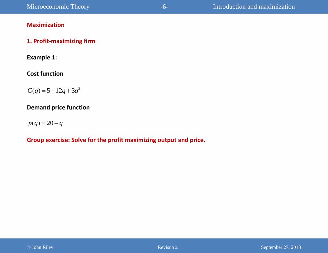
Maximization
1. Profit-maximizing firm
Example 1:
Cost function
2( ) 5 12 3C q q q
Demand price function
( ) 20p q q
Group exercise: Solve for the profit maximizing output and price.
Microeconomic Theory -7- Introduction and maximization
© John Riley Revison 2 September 27, 2018
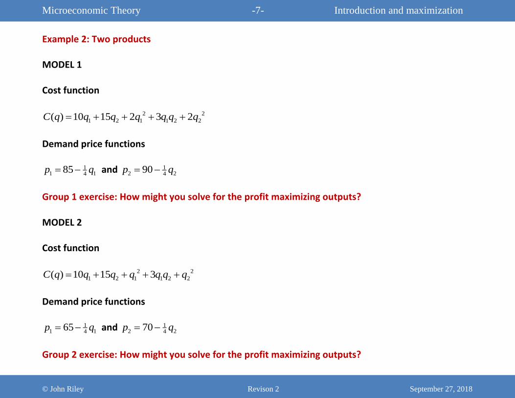
Example 2: Two products
MODEL 1
Cost function
2 2
1 2 1 1 2 2( ) 10 15 2 3 2C q q q q q q q
Demand price functions
11 14
85p q and 12 24
90p q
Group 1 exercise: How might you solve for the profit maximizing outputs?
MODEL 2
Cost function
2 2
1 2 1 1 2 2( ) 10 15 3C q q q q q q q
Demand price functions
11 14
65p q and 12 24
70p q
Group 2 exercise: How might you solve for the profit maximizing outputs?
Microeconomic Theory -8- Introduction and maximization
© John Riley Revison 2 September 27, 2018
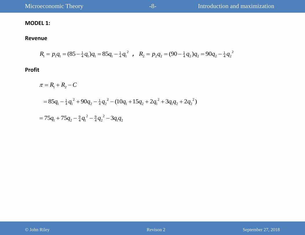
MODEL 1:
Revenue
21 11 1 1 1 1 1 14 4
(85 ) 85R p q q q q q , 21 12 2 2 2 2 2 24 4
(90 ) 90R p q q q q q
Profit
1 2R R C
2 2 2 21 11 1 2 2 1 2 1 1 2 24 4
85 90 (10 15 2 3 2 )q q q q q q q q q q
2 29 91 2 1 2 1 24 4
75 75 3q q q q q q
Microeconomic Theory -9- Introduction and maximization
© John Riley Revison 2 September 27, 2018
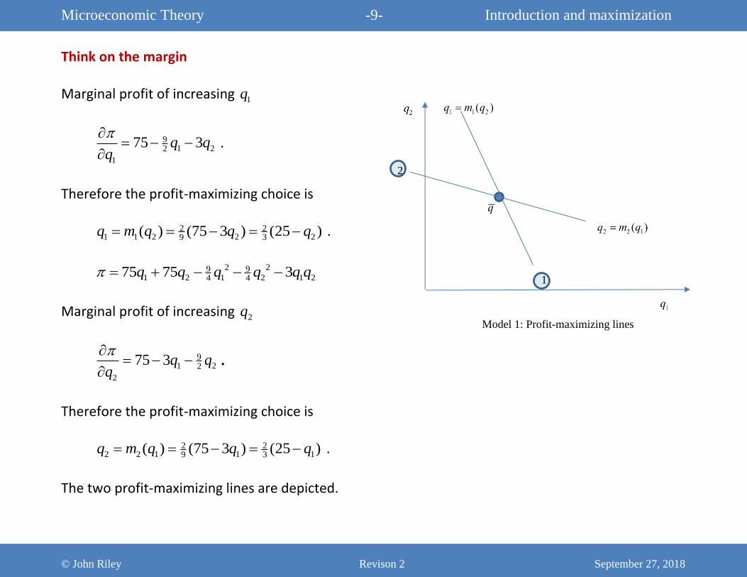
Think on the margin
Marginal profit of increasing 1q
91 22
1
75 3q qq
.
Therefore the profit-maximizing choice is
2 21 1 2 2 29 3
( ) (75 3 ) (25 )q m q q q .
2 29 91 2 1 2 1 24 4
75 75 3q q q q q q
Marginal profit of increasing 2q
91 22
2
75 3q qq
.
Therefore the profit-maximizing choice is
2 22 2 1 1 19 3
( ) (75 3 ) (25 )q m q q q .
The two profit-maximizing lines are depicted.
Model 1: Profit-maximizing lines
1
2
Microeconomic Theory -10- Introduction and maximization
© John Riley Revison 2 September 27, 2018
21 1 2 23
( ) (25 )q m q q , 22 2 1 13
( ) (25 )q m q q
If you solve for q satisfying both equations you will find that the unique solution is
1 2( , ) (10,10)q q q .
Microeconomic Theory -11- Introduction and maximization
© John Riley Revison 2 September 27, 2018
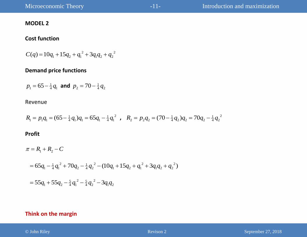
MODEL 2
Cost function
2 2
1 2 1 1 2 2( ) 10 15 3C q q q q q q q
Demand price functions
11 14
65p q and 12 24
70p q
Revenue
21 11 1 1 1 1 1 14 4
(65 ) 65R p q q q q q , 21 12 2 2 2 2 2 24 4
(70 ) 70R p q q q q q
Profit
1 2R R C
2 2 2 21 11 1 2 2 1 2 1 1 2 24 4
65 70 (10 15 3 )q q q q q q q q q q
2 25 51 2 1 2 1 24 4
55 55 3q q q q q q
Think on the margin
Microeconomic Theory -12- Introduction and maximization
© John Riley Revison 2 September 27, 2018
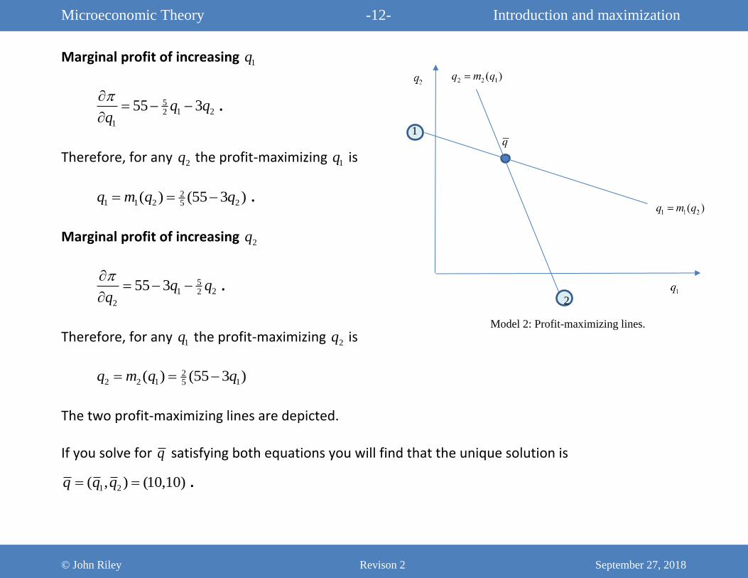
Marginal profit of increasing 1q
51 22
1
55 3q qq
.
Therefore, for any 2q the profit-maximizing 1q is
21 1 2 25
( ) (55 3 )q m q q .
Marginal profit of increasing 2q
51 22
2
55 3q qq
.
Therefore, for any 1q the profit-maximizing 2q is
22 2 1 15
( ) (55 3 )q m q q
The two profit-maximizing lines are depicted.
If you solve for q satisfying both equations you will find that the unique solution is
1 2( , ) (10,10)q q q .
Model 2: Profit-maximizing lines.
2
1
Microeconomic Theory -13- Introduction and maximization
© John Riley Revison 2 September 27, 2018
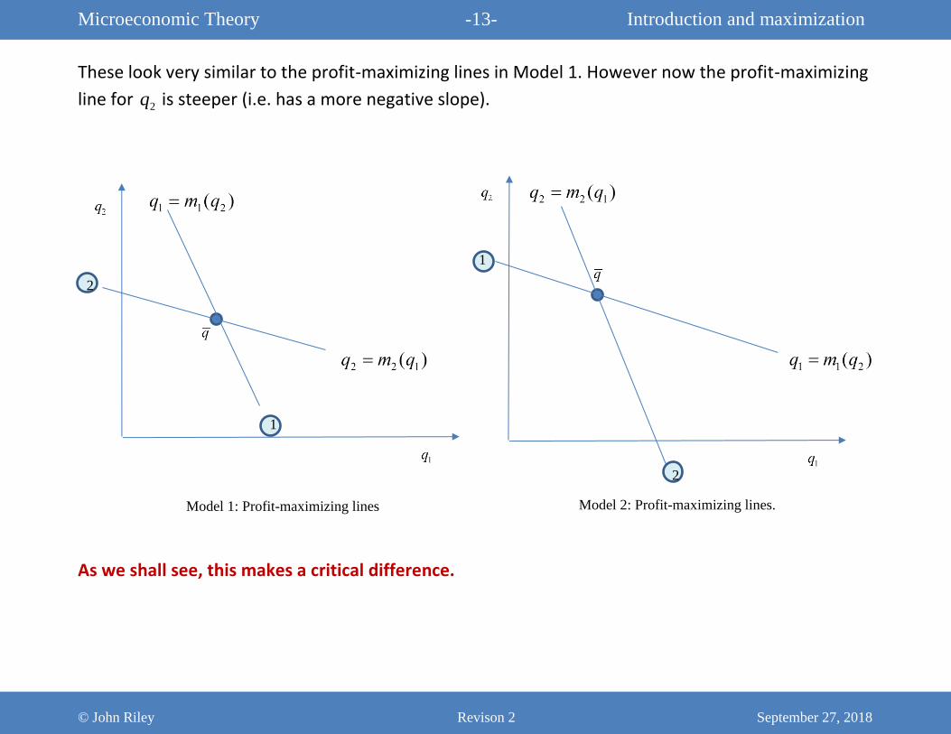
These look very similar to the profit-maximizing lines in Model 1. However now the profit-maximizing
line for 2q is steeper (i.e. has a more negative slope).
As we shall see, this makes a critical difference.
Model 1: Profit-maximizing lines
1
2
Model 2: Profit-maximizing lines.
2
1
Microeconomic Theory -14- Introduction and maximization
© John Riley Revison 2 September 27, 2018
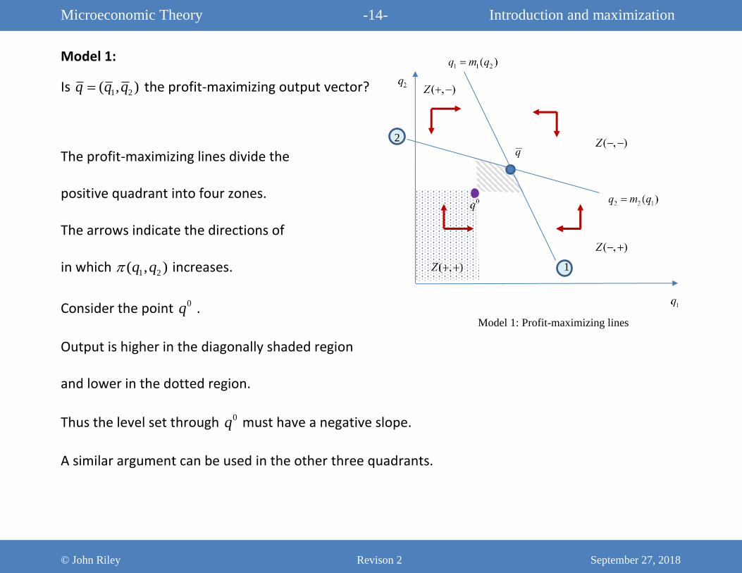
Model 1:
Is 1 2( , )q q q the profit-maximizing output vector?
The profit-maximizing lines divide the
positive quadrant into four zones.
The arrows indicate the directions of
in which 1 2( , )q q increases.
Consider the point 0q .
Output is higher in the diagonally shaded region
and lower in the dotted region.
Thus the level set through 0q must have a negative slope.
A similar argument can be used in the other three quadrants.
Model 1: Profit-maximizing lines
1
2
Microeconomic Theory -15- Introduction and maximization
© John Riley Revison 2 September 27, 2018
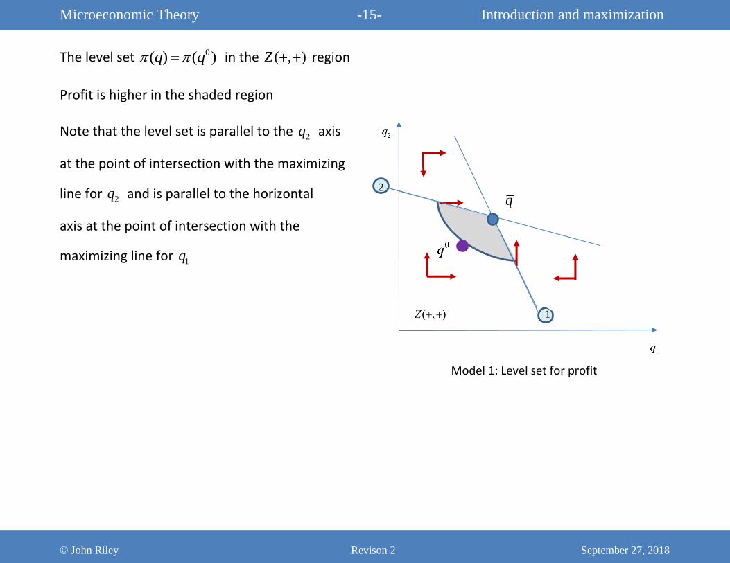
The level set 0( ) ( )q q in the ( , )Z region
Profit is higher in the shaded region
Note that the level set is parallel to the 2q axis
at the point of intersection with the maximizing
line for 2q and is parallel to the horizontal
axis at the point of intersection with the
maximizing line for 1q
Model 1: Level set for profit
1
2
q
Microeconomic Theory -16- Introduction and maximization
© John Riley Revison 2 September 27, 2018
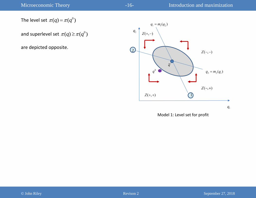
The level set 0( ) ( )q q
and superlevel set 0( ) ( )q q
are depicted opposite.
Model 1: Level set for profit
1
2
Microeconomic Theory -17- Introduction and maximization
© John Riley Revison 2 September 27, 2018
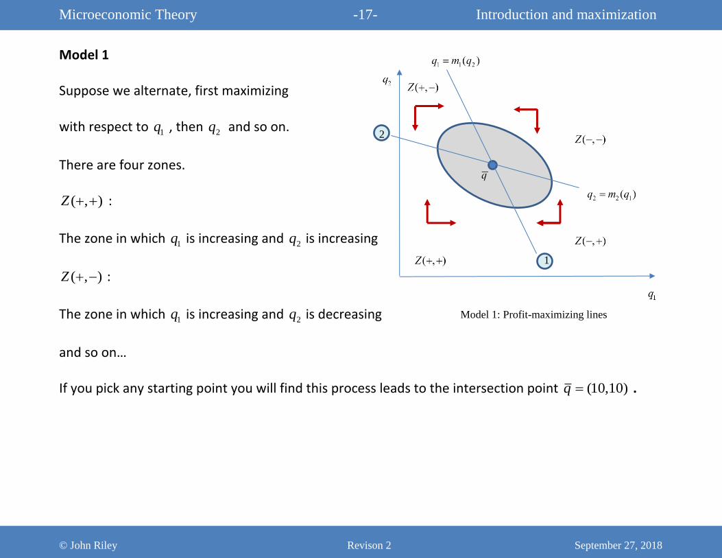
Model 1
Suppose we alternate, first maximizing
with respect to 1q , then 2q and so on.
There are four zones.
( , )Z :
The zone in which 1q is increasing and 2q is increasing
( , )Z :
The zone in which 1q is increasing and 2q is decreasing
and so on…
If you pick any starting point you will find this process leads to the intersection point (10,10)q .
Model 1: Profit-maximizing lines
1
2
Microeconomic Theory -18- Introduction and maximization
© John Riley Revison 2 September 27, 2018
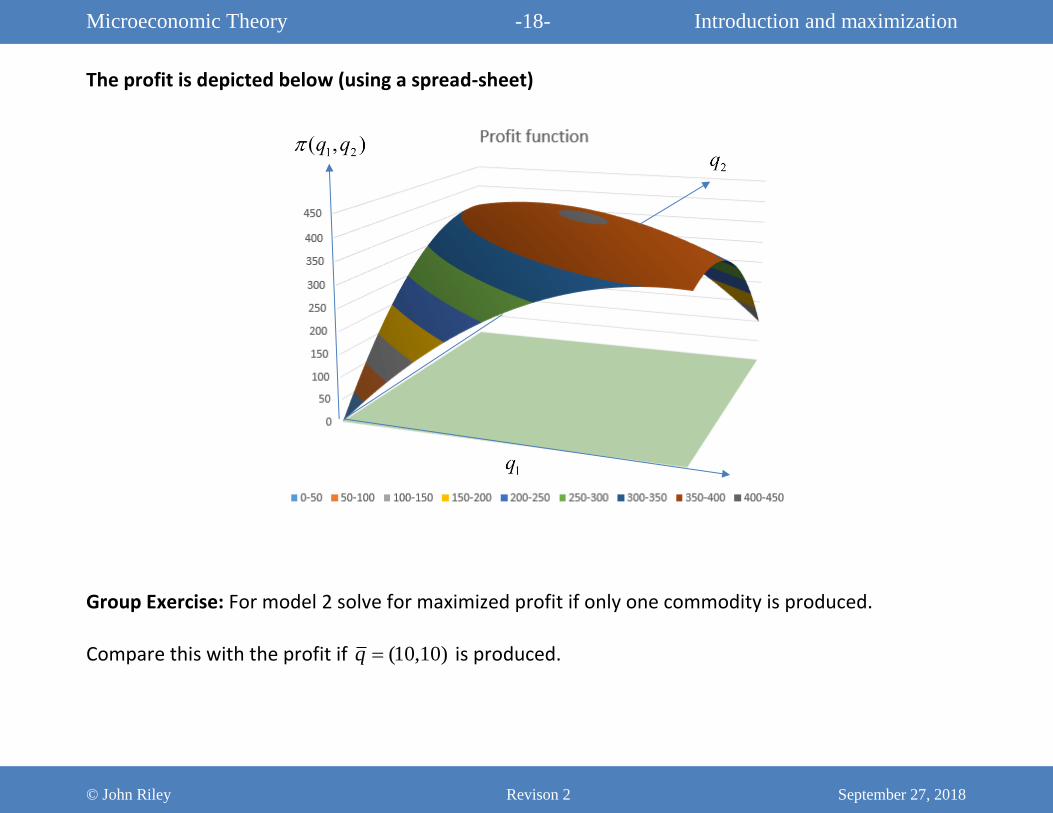
The profit is depicted below (using a spread-sheet)
Group Exercise: For model 2 solve for maximized profit if only one commodity is produced.
Compare this with the profit if (10,10)q is produced.
Microeconomic Theory -19- Introduction and maximization
© John Riley Revison 2 September 27, 2018
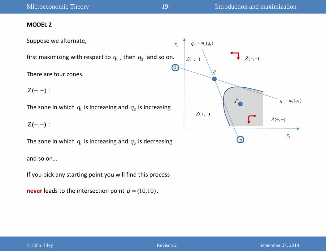
MODEL 2
Suppose we alternate,
first maximizing with respect to 1q , then 2q and so on.
There are four zones.
( , )Z :
The zone in which 1q is increasing and 2q is increasing
( , )Z :
The zone in which 1q is increasing and 2q is decreasing
and so on…
If you pick any starting point you will find this process
never leads to the intersection point (10,10)q .
2
1
Microeconomic Theory -20- Introduction and maximization
© John Riley Revison 2 September 27, 2018
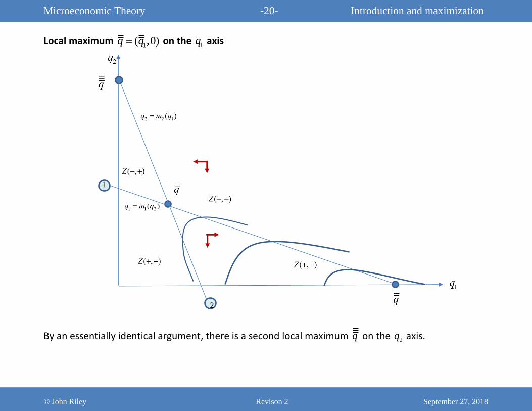
Local maximum 1( ,0)q q on the 1q axis
By an essentially identical argument, there is a second local maximum q on the 2q axis.
2
1
Microeconomic Theory -21- Introduction and maximization
© John Riley Revison 2 September 27, 2018
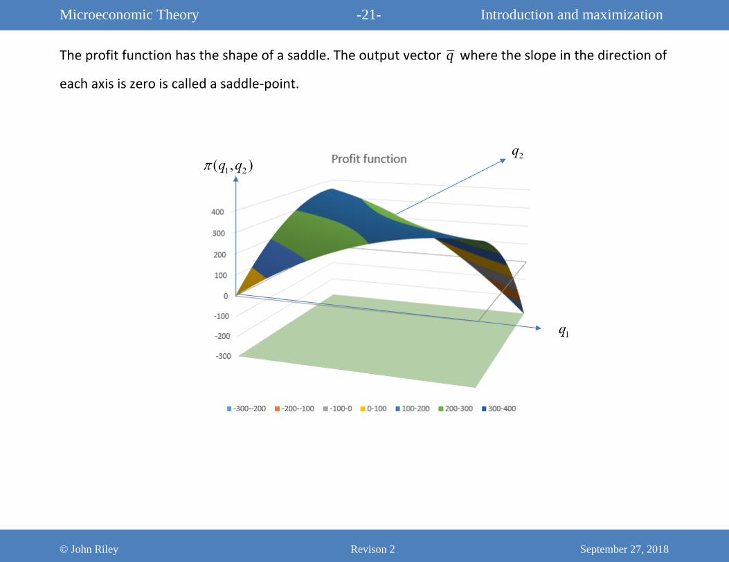
The profit function has the shape of a saddle. The output vector q where the slope in the direction of
each axis is zero is called a saddle-point.
Microeconomic Theory -22- Introduction and maximization
© John Riley Revison 2 September 27, 2018
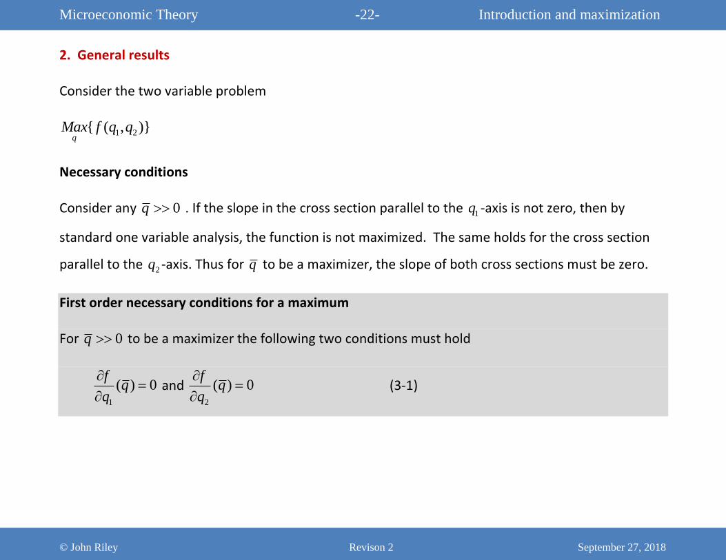
2. General results
Consider the two variable problem
1 2{ ( , )}q
Max f q q
Necessary conditions
Consider any 0q . If the slope in the cross section parallel to the 1q -axis is not zero, then by
standard one variable analysis, the function is not maximized. The same holds for the cross section
parallel to the 2q -axis. Thus for q to be a maximizer, the slope of both cross sections must be zero.
First order necessary conditions for a maximum
For 0q to be a maximizer the following two conditions must hold
1
( ) 0f
and
2
( ) 0f
(3-1)
Microeconomic Theory -23- Introduction and maximization
© John Riley Revison 2 September 27, 2018
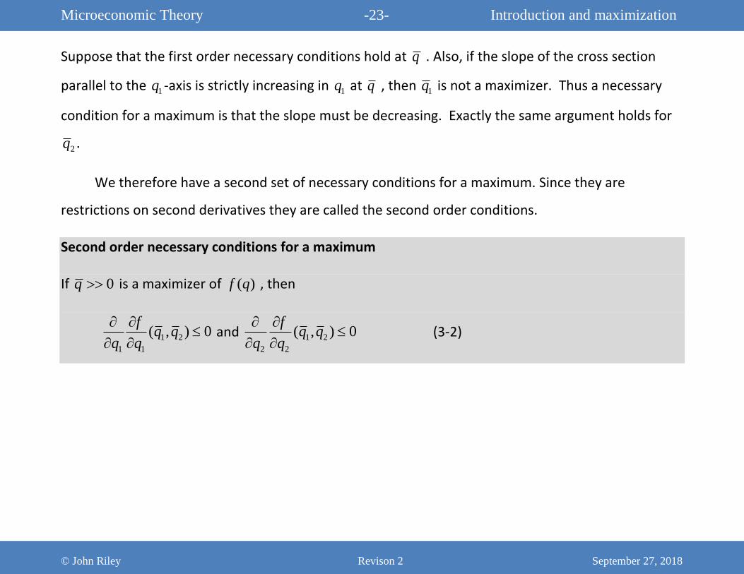
Suppose that the first order necessary conditions hold at q . Also, if the slope of the cross section
parallel to the 1q -axis is strictly increasing in 1q at q , then 1q is not a maximizer. Thus a necessary
condition for a maximum is that the slope must be decreasing. Exactly the same argument holds for
2q .
We therefore have a second set of necessary conditions for a maximum. Since they are
restrictions on second derivatives they are called the second order conditions.
Second order necessary conditions for a maximum
If 0q is a maximizer of ( )f q , then
1 2
1 1
( , ) 0f
q qq q
and 1 2
2 2
( , ) 0f
q qq q
(3-2)
Microeconomic Theory -24- Introduction and maximization
© John Riley Revison 2 September 27, 2018
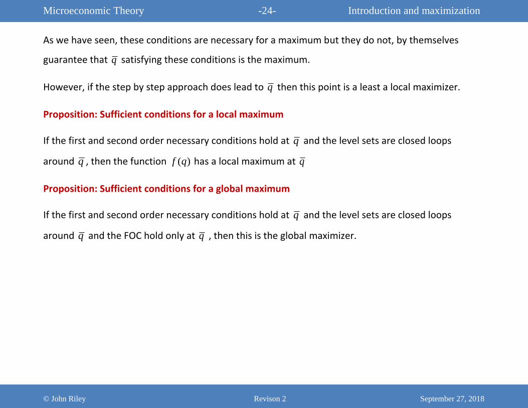
As we have seen, these conditions are necessary for a maximum but they do not, by themselves
guarantee that q satisfying these conditions is the maximum.
However, if the step by step approach does lead to q then this point is a least a local maximizer.
Proposition: Sufficient conditions for a local maximum
If the first and second order necessary conditions hold at q and the level sets are closed loops
around q , then the function ( )f q has a local maximum at q
Proposition: Sufficient conditions for a global maximum
If the first and second order necessary conditions hold at q and the level sets are closed loops
around q and the FOC hold only at q , then this is the global maximizer.
Microeconomic Theory -25- Introduction and maximization
© John Riley Revison 2 September 27, 2018
3. Non-negativity constraints
Many economic variables cannot be negative. Suppose this is true for all variables
Let 1( ,..., )nx x x solve 0
{ ( )}x
Max f x
.
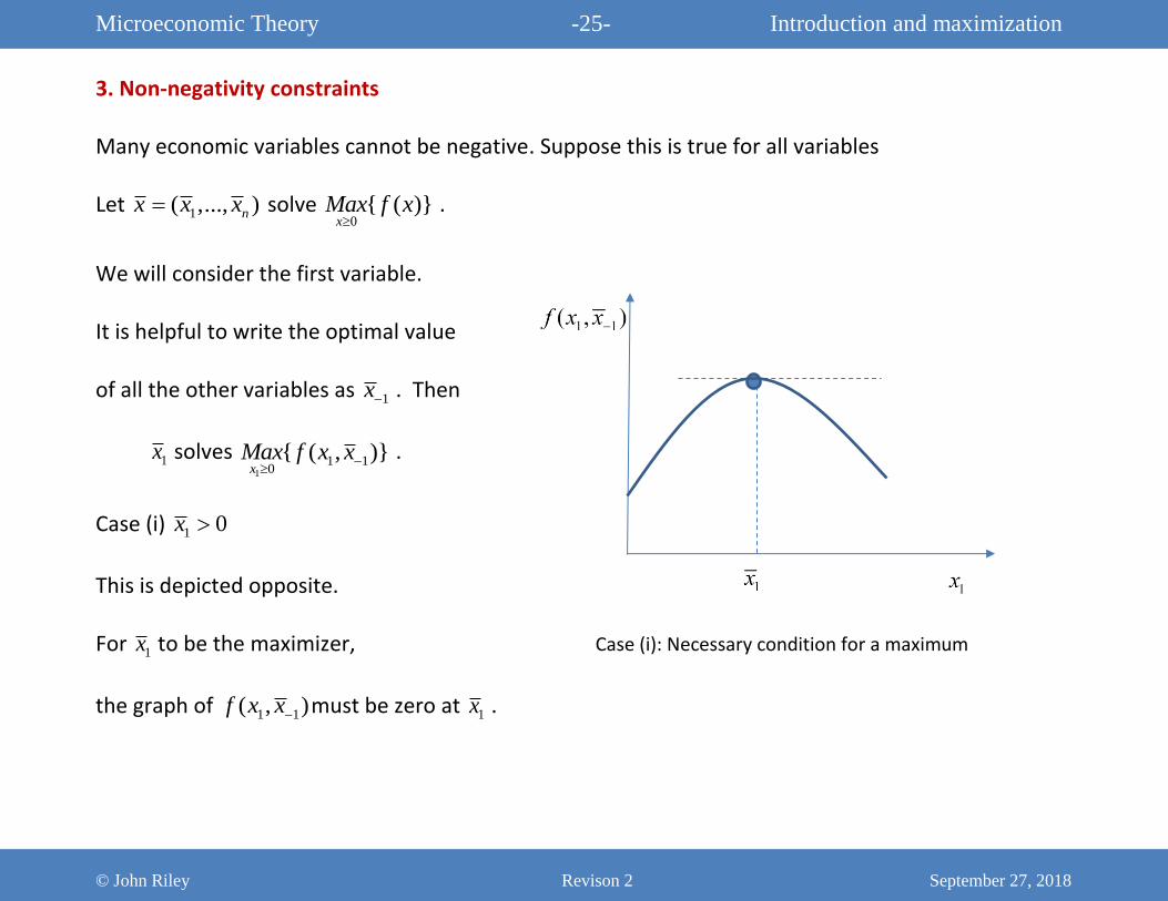
We will consider the first variable.
It is helpful to write the optimal value
of all the other variables as 1x . Then
1x solves 1
1 10
{ ( , )}x
Max f x x
.
Case (i) 1 0x
This is depicted opposite.
For 1x to be the maximizer,
the graph of 1 1( , )f x x must be zero at 1x .
Case (i): Necessary condition for a maximum
Microeconomic Theory -26- Introduction and maximization
© John Riley Revison 2 September 27, 2018
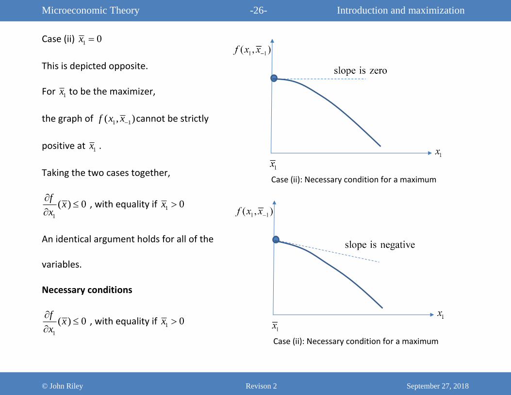
Case (ii) 1 0x
This is depicted opposite.
For 1x to be the maximizer,
the graph of 1 1( , )f x x cannot be strictly
positive at 1x .
Taking the two cases together,
1
( ) 0f
xx
, with equality if 1 0x
An identical argument holds for all of the
variables.
Necessary conditions
1
( ) 0f
xx
, with equality if 1 0x
Case (ii): Necessary condition for a maximum
Case (ii): Necessary condition for a maximum
Microeconomic Theory -27- Introduction and maximization
© John Riley Revison 2 September 27, 2018
4. Laws of supply and input demand
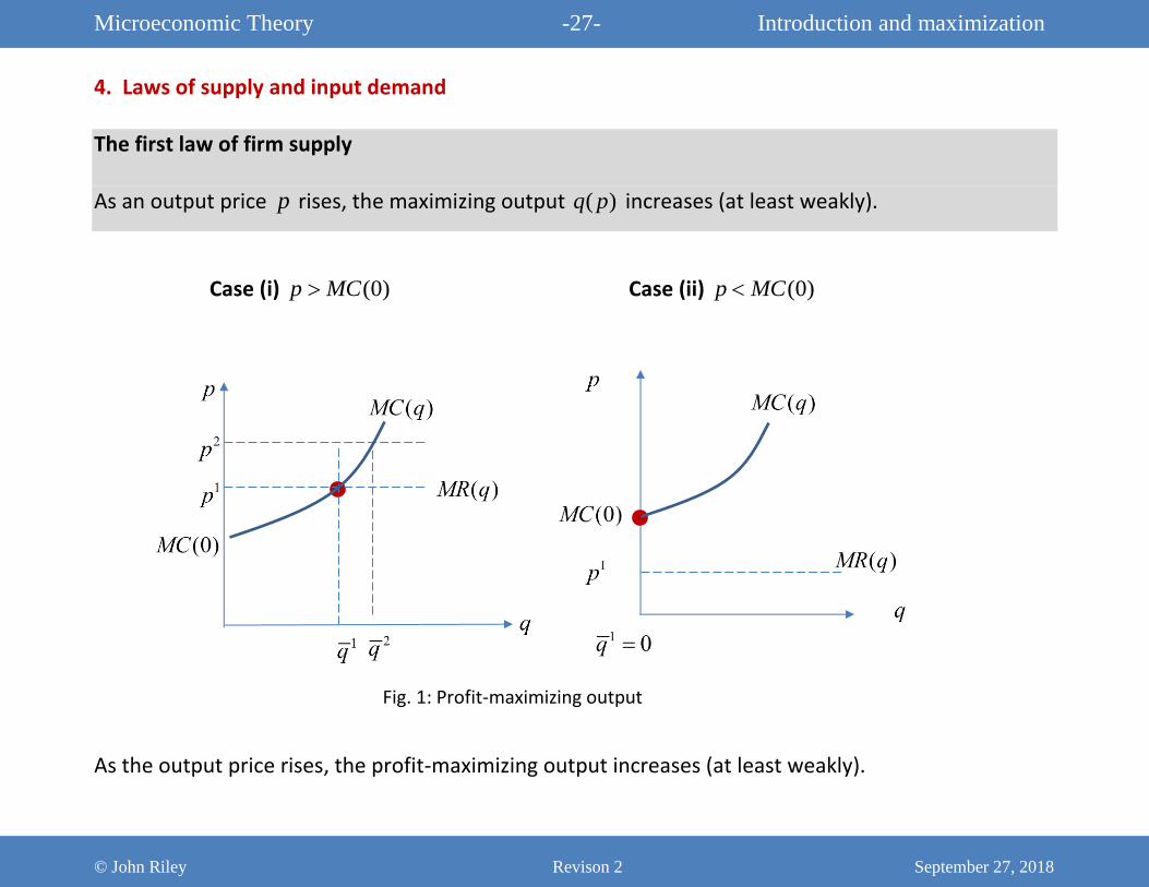
The first law of firm supply
As an output price p rises, the maximizing output ( )q p increases (at least weakly).
Case (i) (0)p MC Case (ii) (0)p MC
As the output price rises, the profit-maximizing output increases (at least weakly).
Fig. 1: Profit-maximizing output
Microeconomic Theory -28- Introduction and maximization
© John Riley Revison 2 September 27, 2018
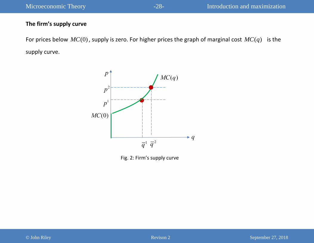
The firm’s supply curve
For prices below (0)MC , supply is zero. For higher prices the graph of marginal cost ( )MC q is the
supply curve.
Fig. 2: Firm’s supply curve
Microeconomic Theory -29- Introduction and maximization
© John Riley Revison 2 September 27, 2018
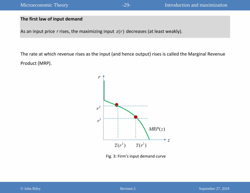
The first law of input demand
As an input price r rises, the maximizing input ( )z r decreases (at least weakly).
The rate at which revenue rises as the input (and hence output) rises is called the Marginal Revenue
Product (MRP).
Fig. 3: Firm’s input demand curve
Microeconomic Theory -30- Introduction and maximization
© John Riley Revison 2 September 27, 2018
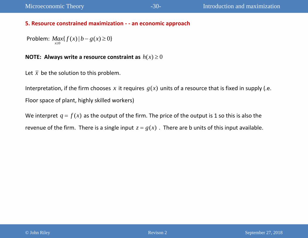
5. Resource constrained maximization - - an economic approach
Problem: 0
{ ( ) | ( ) 0}x
Max f x b g x
NOTE: Always write a resource constraint as ( ) 0h x
Let x be the solution to this problem.
Interpretation, if the firm chooses x it requires ( )g x units of a resource that is fixed in supply (.e.
Floor space of plant, highly skilled workers)
We interpret ( )q f x as the output of the firm. The price of the output is 1 so this is also the
revenue of the firm. There is a single input ( )z g x . There are b units of this input available.
Microeconomic Theory -31- Introduction and maximization
© John Riley Revison 2 September 27, 2018
To solve this problem, we consider the “relaxed problem” in which the firm can purchase additional
units at the price . Since this is a hypothetical opportunity, economists refer to the price as the
“shadow price” of the resource rather than a market price.
Suppose that the firm purchases ( )g x b additional units. Its profit is then
( ) ( ( ) ) ( ) ( ( ))f x g x b f x b g x L
The relaxed problem is then
0
{ ( ) ( ( ))}x
Max f x b g x
L
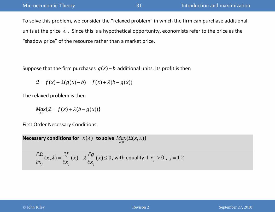
First Order Necessary Conditions:
Necessary conditions for ( )x to solve 0
{ ( , )}x
Max x L
( , ) ( ) ( ) 0j j j
f gx x x
x x x
L, with equality if 0jx , 1,2j
Microeconomic Theory -32- Introduction and maximization
© John Riley Revison 2 September 27, 2018
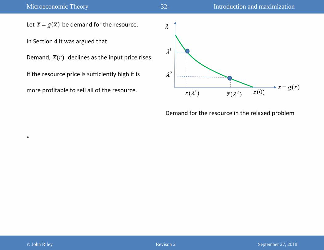
Let ( )z g x be demand for the resource.
In Section 4 it was argued that
Demand, ( )z r declines as the input price rises.
If the resource price is sufficiently high it is
more profitable to sell all of the resource.
*
Demand for the resource in the relaxed problem
Microeconomic Theory -33- Introduction and maximization
© John Riley Revison 2 September 27, 2018
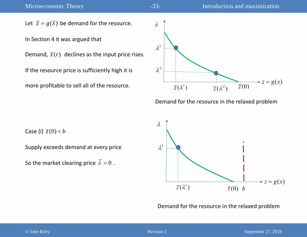
Let ( )z g x be demand for the resource.
In Section 4 it was argued that
Demand, ( )z r declines as the input price rises.
If the resource price is sufficiently high it is
more profitable to sell all of the resource.
Case (i) (0)z b
Supply exceeds demand at every price
So the market clearing price 0 .
Demand for the resource in the relaxed problem
Demand for the resource in the relaxed problem
Microeconomic Theory -34- Introduction and maximization
© John Riley Revison 2 September 27, 2018
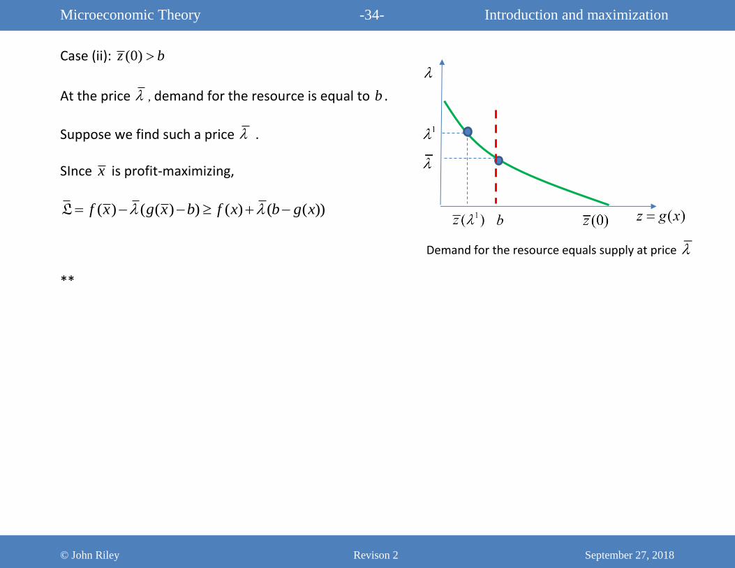
Case (ii): (0)z b
At the price , demand for the resource is equal to b .
Suppose we find such a price .
SInce x is profit-maximizing,
( ) ( ( ) ) ( ) ( ( ))f x g x b f x b g x L
**
Demand for the resource equals supply at price
Microeconomic Theory -35- Introduction and maximization
© John Riley Revison 2 September 27, 2018
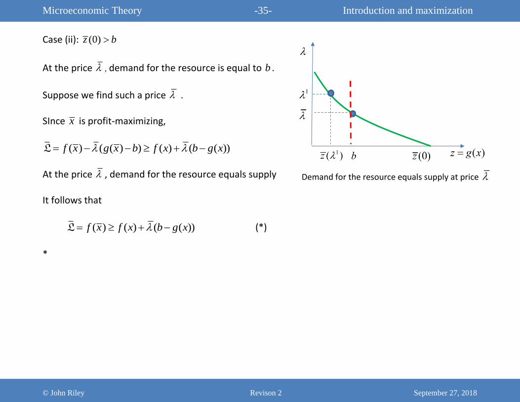
Case (ii): (0)z b
At the price , demand for the resource is equal to b .
Suppose we find such a price .
SInce x is profit-maximizing,
( ) ( ( ) ) ( ) ( ( ))f x g x b f x b g x L
At the price , demand for the resource equals supply
It follows that
( ) ( ) ( ( ))f x f x b g x L (*)
*
Demand for the resource equals supply at price
Microeconomic Theory -36- Introduction and maximization
© John Riley Revison 2 September 27, 2018
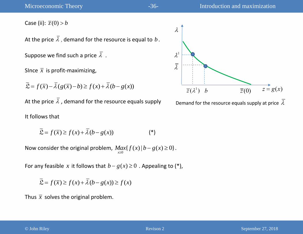
Case (ii): (0)z b
At the price , demand for the resource is equal to b .
Suppose we find such a price .
SInce x is profit-maximizing,
( ) ( ( ) ) ( ) ( ( ))f x g x b f x b g x L
At the price , demand for the resource equals supply
It follows that
( ) ( ) ( ( ))f x f x b g x L (*)
Now consider the original problem, 0
{ ( ) | ( ) 0}x
Max f x b g x
.
For any feasible x it follows that ( ) 0b g x . Appealing to (*),
( ) ( ) ( ( )) ( )f x f x b g x f x L
Thus x solves the original problem.
Demand for the resource equals supply at price
Microeconomic Theory -37- Introduction and maximization
© John Riley Revison 2 September 27, 2018
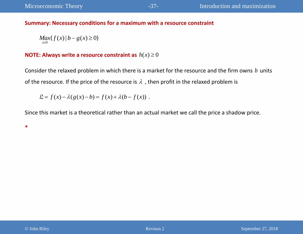
Summary: Necessary conditions for a maximum with a resource constraint
0{ ( ) | ( ) 0}
xMax f x b g x
NOTE: Always write a resource constraint as ( ) 0h x
Consider the relaxed problem in which there is a market for the resource and the firm owns b units
of the resource. If the price of the resource is , then profit in the relaxed problem is
( ) ( ( ) ) ( ) ( ( ))f x g x b f x b f x L .
Since this market is a theoretical rather than an actual market we call the price a shadow price.
*
Microeconomic Theory -38- Introduction and maximization
© John Riley Revison 2 September 27, 2018
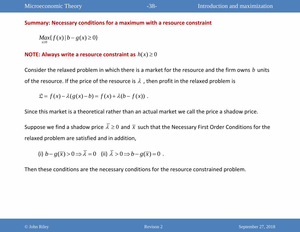
Summary: Necessary conditions for a maximum with a resource constraint
0{ ( ) | ( ) 0}
xMax f x b g x
NOTE: Always write a resource constraint as ( ) 0h x
Consider the relaxed problem in which there is a market for the resource and the firm owns b units
of the resource. If the price of the resource is , then profit in the relaxed problem is
( ) ( ( ) ) ( ) ( ( ))f x g x b f x b f x L .
Since this market is a theoretical rather than an actual market we call the price a shadow price.
Suppose we find a shadow price 0 and x such that the Necessary First Order Conditions for the
relaxed problem are satisfied and in addition,
(i) ( ) 0 0b g x (ii) 0 ( ) 0b g x .
Then these conditions are the necessary conditions for the resource constrained problem.
Microeconomic Theory -39- Introduction and maximization
© John Riley Revison 2 September 27, 2018
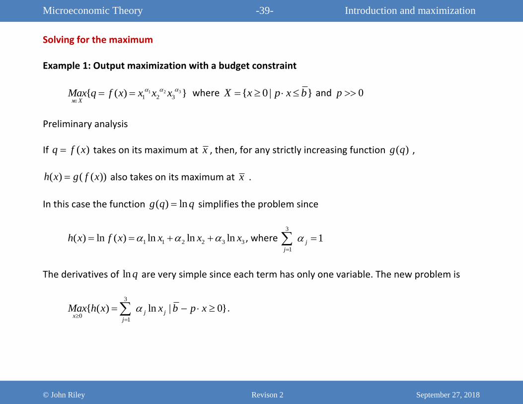
Solving for the maximum
Example 1: Output maximization with a budget constraint
31 2
1 2 3{ ( ) }x X
Max q f x x x x
where { 0 | }X x p x b and 0p
Preliminary analysis
If ( )q f x takes on its maximum at x , then, for any strictly increasing function ( )g q ,
( ) ( ( ))h x g f x also takes on its maximum at x .
In this case the function ( ) lng q q simplifies the problem since
1 1 2 2 3 3( ) ln ( ) ln ln lnh x f x x x x , where 3
1
1j
j
The derivatives of ln q are very simple since each term has only one variable. The new problem is
3
01
{ ( ) ln | 0}j jx
j
Max h x x b p x
.
Microeconomic Theory -40- Introduction and maximization
© John Riley Revison 2 September 27, 2018
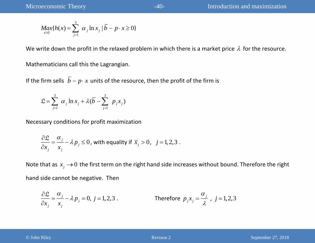
3
01
{ ( ) ln | 0}j jx
j
Max h x x b p x
We write down the profit in the relaxed problem in which there is a market price for the resource.
Mathematicians call this the Lagrangian.
If the firm sells b p x units of the resource, then the profit of the firm is
3 3
1 1
ln ( )j j j j
j j
x b p x
L
Necessary conditions for profit maximization
0j
j
j j
px x
L, with equality if 0jx , 1,2,3j .
Note that as 0jx the first term on the right hand side increases without bound. Therefore the right
hand side cannot be negative. Then
0,j
j
j j
px x
L1,2,3j . Therefore
j
j jp x
, 1,2,3j
Microeconomic Theory -41- Introduction and maximization
© John Riley Revison 2 September 27, 2018
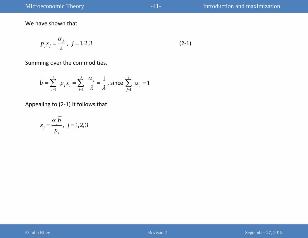
We have shown that
j
j jp x
, 1,2,3j (2-1)
Summing over the commodities,
3 3
1 1
1j
j j
j j
b p x
, since 3
1
1j
j
Appealing to (2-1) it follows that
j
j
j
bx
p
, 1,2,3j
Microeconomic Theory -42- Introduction and maximization
© John Riley Revison 2 September 27, 2018
Example 2: Utility maximization
A consumer’s preferences are represented by a strictly increasing utility function ( )U x , where
( ) 0U x if and only if 0x . The consumer’s budget constraint is 1 1 ... n np x p x p x I where
the price vector 0p .
The consumer chooses x to solve 0
{ ( ) | }x
Max U x p x I
.
Group Exercise:
(1) Explain why 0x and p x I
(ii) Show that the FOC can be written as follows:
1
1
... n
n
UU
xx
p p
.
(iii) Provide the intuition behind these conditions.
Microeconomic Theory -43- Introduction and maximization
© John Riley Revison 2 September 27, 2018
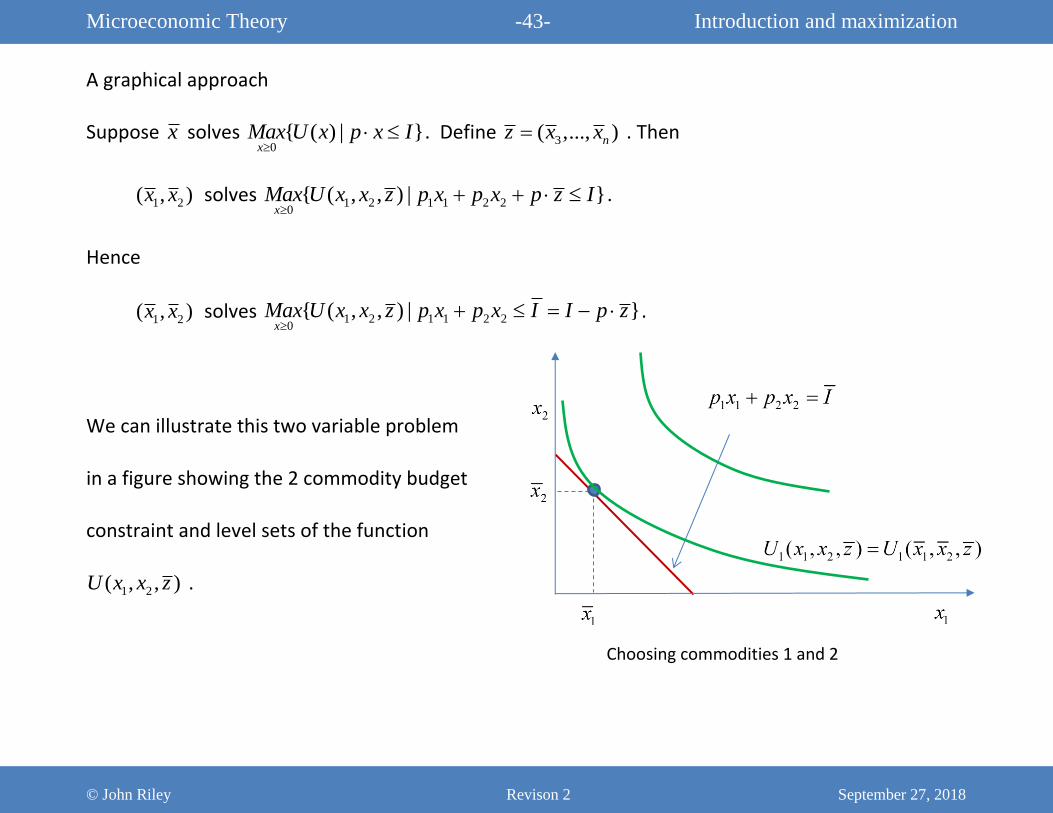
A graphical approach
Suppose x solves 0
{ ( ) | }x
Max U x p x I
. Define 3( ,..., )nz x x . Then
1 2( , )x x solves 1 2 1 1 2 20
{ ( , , ) | }x
Max U x x z p x p x p z I
.
Hence
1 2( , )x x solves 1 2 1 1 2 20
{ ( , , ) | }x
Max U x x z p x p x I I p z
.
We can illustrate this two variable problem
in a figure showing the 2 commodity budget
constraint and level sets of the function
1 2( , , )U x x z .
Choosing commodities 1 and 2
Microeconomic Theory -44- Introduction and maximization
© John Riley Revison 2 September 27, 2018
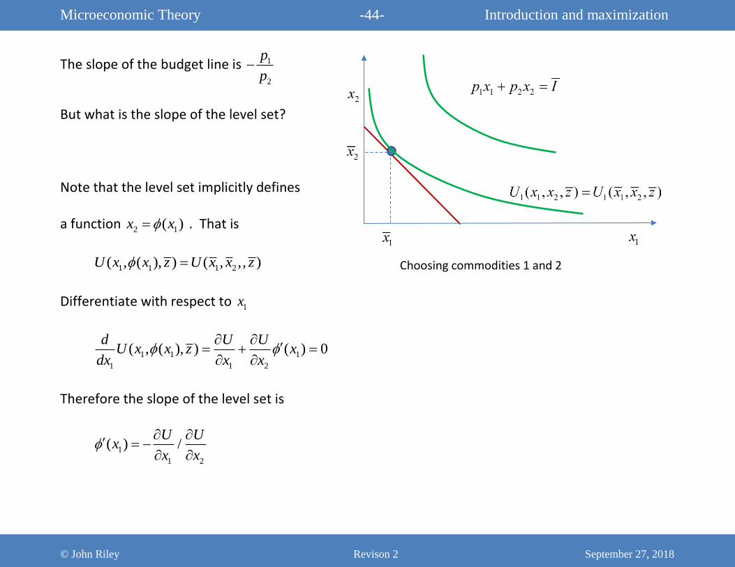
The slope of the budget line is 1
2
p
p
But what is the slope of the level set?
Note that the level set implicitly defines
a function 2 1( )x x . That is
1 1 1 2( , ( ), ) ( , ,, )U x x z U x x z
Differentiate with respect to 1x
1 1 1
1 1 2
( , ( ), ) ( ) 0d U U
U x x z xdx x x
Therefore the slope of the level set is
1
1 2
( ) /U U
xx x
Choosing commodities 1 and 2
Microeconomic Theory -45- Introduction and maximization
© John Riley Revison 2 September 27, 2018
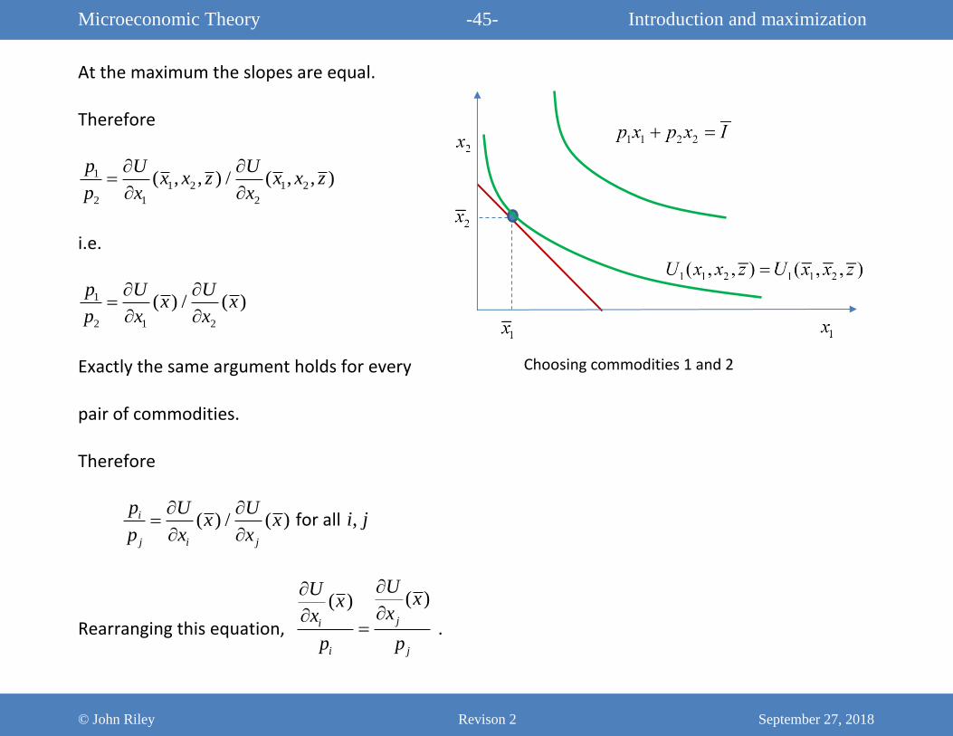
At the maximum the slopes are equal.
Therefore
11 2 1 2
2 1 2
( , , ) / ( , , )p U U
x x z x x zp x x
i.e.
1
2 1 2
( ) / ( )p U U
x xp x x
Exactly the same argument holds for every
pair of commodities.
Therefore
( ) / ( )i
j i j
p U Ux x
p x x
for all ,i j
Rearranging this equation,
( )( )ji
i j
UUxx
xx
p p
.
Choosing commodities 1 and 2