Phys 112 (F2006) 3 Equilibrium between 2 systems B. Sadoulet1

3 Equilibrium Between Two Systems

Chapter 2 Kittel&Kroemer“Microcanonical methods”

3.1 Equilibrium between 2 systems3.2 Temperature, pressure, chemical potential

Definition

3.3 Ideal gas3.4 Thermodynamics identities

The three lawsS,U,H,F,GA note about differentials

3.5 Chemical PotentialWhy is the Chemical Potential a potentialWhy is it call “Chemical”

Phys 112 (F2006) 3 Equilibrium between 2 systems B. Sadoulet2

Let us consider a gasConstraints: Energy U

Volume V Note: AdditiveNumber of particles of species i : Ni

Take 2 systems and put them in contact Put them in weak interactions Isolated=> fixed U,V,N

Configuration described by U1,V1,Ni1

Weak interaction => (quantum) states not modified multiplicity function =product of multiplicity functions

More states => Entropy increases

U = U1 +U2V = V1 +V2Ni = Ni1 + Ni2

U1,V1, Ni1 U2 ,V2 , Ni2

3.1 Thermal equilibrium between 2 Systems

g U1,V1, Ni1( ) = g1 U1,V1, Ni1( )g2 U −U1,V −V1, Ni − Ni1( )

Phys 112 (F2006) 3 Equilibrium between 2 systems B. Sadoulet3

Thermal equilibrium between 2 Systems

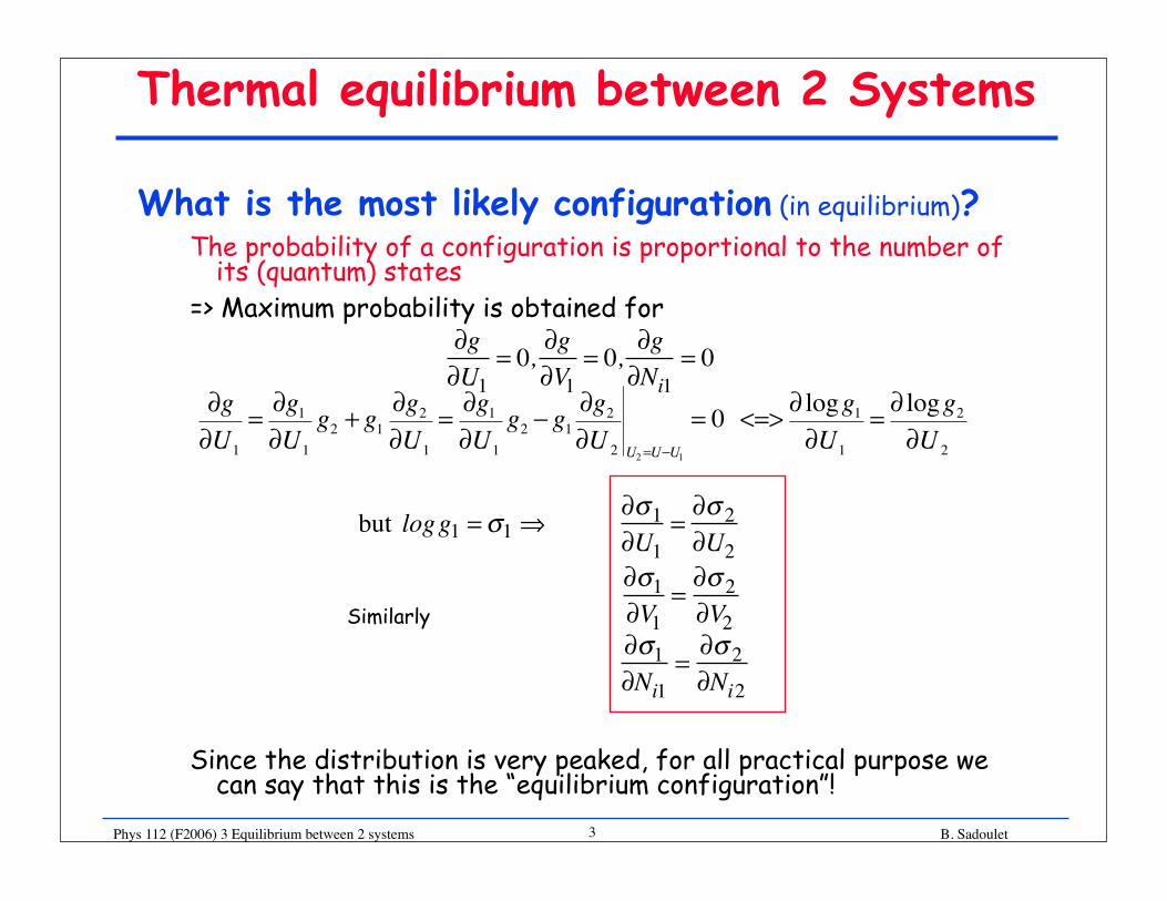
What is the most likely configuration (in equilibrium)?The probability of a configuration is proportional to the number of

its (quantum) states => Maximum probability is obtained for

Similarly

Since the distribution is very peaked, for all practical purpose we can say that this is the “equilibrium configuration”!

∂g∂U1

= 0, ∂g∂V1

= 0, ∂g∂Ni1

= 0

�

∂g∂U1

= ∂g1

∂U1

g2 + g1∂g2

∂U1

= ∂g1

∂U1

g2 − g1∂g2

∂U 2 U2 =U−U1

= 0 <=> ∂ logg1

∂U1

= ∂ logg2

∂U 2

but logg1 =σ1 ⇒ ∂σ1∂U1

=∂σ 2∂U2

∂σ1∂V1

=∂σ 2∂V2

∂σ1∂Ni1

=∂σ 2∂Ni2

Phys 112 (F2006) 3 Equilibrium between 2 systems B. Sadoulet4

Graphic Representation

Watch outNumber of states of the

combined system is the product of the number of states of each system

Most likely configuration= the configuration with thelargest number of states

g1 g2

U1

g1 U1( )g2 U −U1( )

g1 U1( )g2 U −U1( )

UMost likelyU1

log g1 log g2

U1

UMost likely

U1

∂ logg1 U1( )∂U1

= −∂ logg2 U −U1( )

∂U1

=∂ logg2 U2( )

∂U2 U2 =U −U1

Phys 112 (F2006) 3 Equilibrium between 2 systems B. Sadoulet5

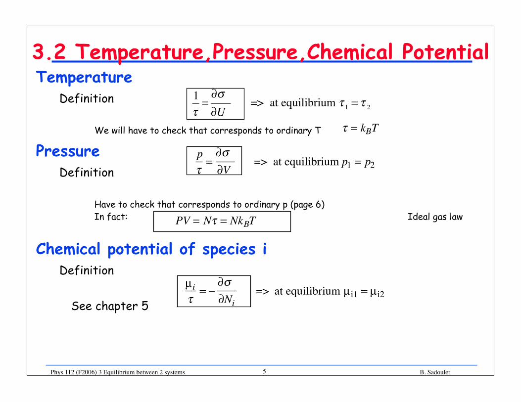
3.2 Temperature,Pressure,Chemical PotentialTemperature

Definition

We will have to check that corresponds to ordinary T

PressureDefinition

Have to check that corresponds to ordinary p (page 6)In fact: Ideal gas law

Chemical potential of species iDefinition

See chapter 5

τ = kBT

�

1τ

=∂σ∂U

=> at equilibrium τ 1 = τ 2

pτ=∂σ∂V

=> at equilibrium p1 = p2

PV = Nτ = NkBT

µiτ

= −∂σ∂Ni

=> at equilibrium µi1 = µi2

Phys 112 (F2006) 3 Equilibrium between 2 systems B. Sadoulet6

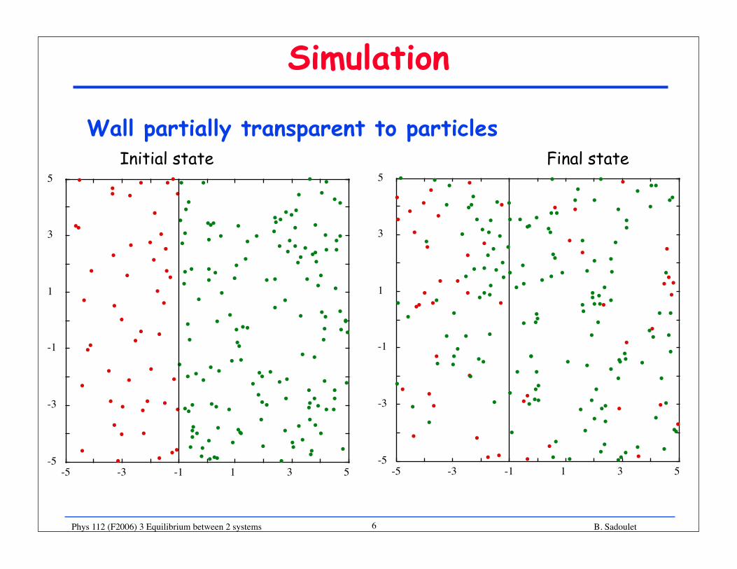
Simulation

Wall partially transparent to particlesInitial state Final state

-5

-3

-1

1

3

5

-5 -3 -1 1 3 5-5

-3

-1

1

3

5

-5 -3 -1 1 3 5

Phys 112 (F2006) 3 Equilibrium between 2 systems B. Sadoulet7

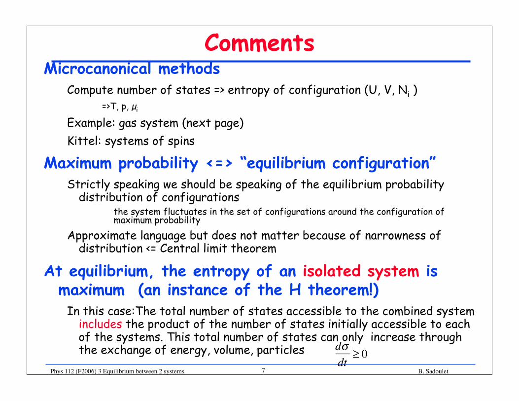
CommentsMicrocanonical methods

Compute number of states => entropy of configuration (U, V, Ni )=>T, p, µi

Example: gas system (next page)Kittel: systems of spins

Maximum probability <=> “equilibrium configuration”Strictly speaking we should be speaking of the equilibrium probability

distribution of configurations the system fluctuates in the set of configurations around the configuration of

maximum probability

Approximate language but does not matter because of narrowness of distribution <= Central limit theorem

At equilibrium, the entropy of an isolated system is maximum (an instance of the H theorem!)

In this case:The total number of states accessible to the combined system includes the product of the number of states initially accessible to each of the systems. This total number of states can only increase through the exchange of energy, volume, particles dσ

dt≥ 0

Phys 112 (F2006) 3 Equilibrium between 2 systems B. Sadoulet8

3.3 Ideal GasCheck that our definitions are OK. Not in Kittel& Kroemer. cf Reif 2.5

Calculation of entropy as a function of UDone in Chapter 2 of the notes slide 13

Temperature

this is the classical result (3/2 kB T per spinless monoatomic particle)

Pressure

Law of ideal gases! Reassuring!Illustrates the power of microcanonical methods (at the price of often

difficult computations of the multiplicity of states)

1τ=∂σ∂U

=3N2U

⇒U =32

Nτ =32

NkBT

pτ=∂σ∂V

=NV

⇒ pV = Nτ = NkBT

for large N g ∝V NU3N2 σ = f N( ) + N logV + 3 / 2N logU

Phys 112 (F2006) 3 Equilibrium between 2 systems B. Sadoulet9

Is the pressure the force per unit area? cf. Kittel and Kroemer Chapter 14 p. 391

Describe the particles by their individual density in momentum space (ideal gas)

If the particles have specular reflection by the wall, the momentum transfer for a particle arriving at angle θ is

Integration on angles gives

that we would like to compare with the energy density

θ

�

non relativistic⇒ pv = 2ε ⇒ pressure P = 23u (energy density)

u = 32NVτ ⇒ P = N

Vτ = same pressure as thermodynamic definition = τ∂σ

∂V U,Nultra relativistic ⇒ pv = ε ⇒ P =

13u

2 pcosθ

�

23× 2π pv n p( )p 2dp

0

∞∫

!

�

u = ε n p( )d 3 p0

∞∫ = 4π ε n p( )p 2dp0

∞∫

density in d 3p = n p( ) p2dpdΩ

vΔt

dA

P =ForcedA

=d ΔpΔtdA

=1

dAΔt2pcosθ

Momentum transfer

vΔtdAcosθVolume of cylinder n p( ) p2dpdΩ

density in cylinder ∫

= dϕ0

2π

∫ d cosθ 2pvcos2θ n p( ) p2dp0

∞

∫0

1

∫

Phys 112 (F2006) 3 Equilibrium between 2 systems B. Sadoulet10

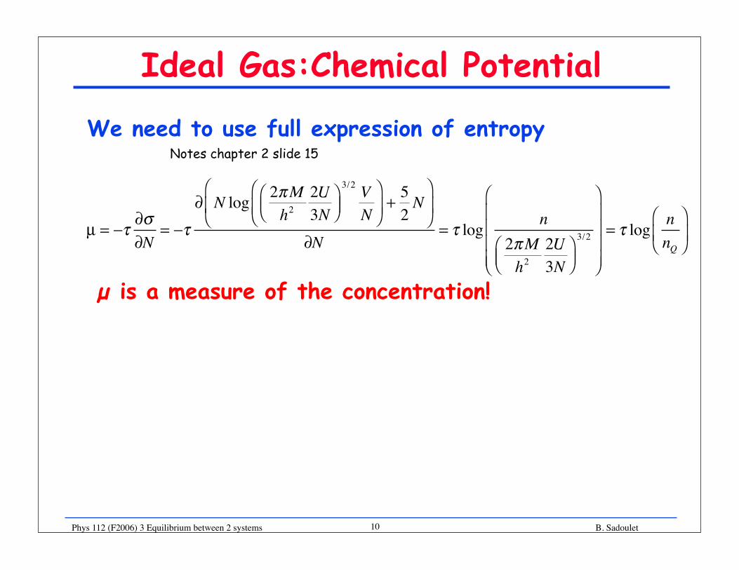
Ideal Gas:Chemical Potential

We need to use full expression of entropy Notes chapter 2 slide 15

µ is a measure of the concentration!

µ = −τ ∂σ∂N

= −τ∂ N log 2πM

h22U3N

⎛⎝⎜

⎞⎠⎟3/2 VN

⎛

⎝⎜⎞

⎠⎟+ 52N

⎛

⎝⎜

⎞

⎠⎟

∂N= τ log n

2πMh2

2U3N

⎛⎝⎜

⎞⎠⎟3/2

⎛

⎝

⎜⎜⎜⎜

⎞

⎠

⎟⎟⎟⎟

= τ log nnQ

⎛

⎝⎜⎞

⎠⎟

Phys 112 (F2006) 3 Equilibrium between 2 systems B. Sadoulet

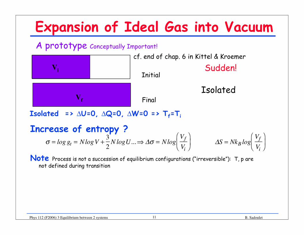
Isolated => ΔU=0, ΔQ=0, ΔW=0 => Tf=Ti

Increase of entropy ?

Note Process is not a succession of equilibrium configurations (“irreversible”): T, p are not defined during transition

11

Expansion of Ideal Gas into VacuumA prototype Conceptually Important!

cf. end of chap. 6 in Kittel & Kroemer

Initial

FinalIsolated

Vi

Vf

σ = log gt = NlogV +32N logU...⇒Δσ = Nlog

VfVi

⎛ ⎝ ⎜

⎞ ⎠ ⎟ ΔS = NkB log

VfVi

⎛ ⎝ ⎜

⎞ ⎠ ⎟

Sudden!

Phys 112 (F2006) 3 Equilibrium between 2 systems B. Sadoulet12

3.4Thermodynamics IdentitiesZeroth Law

Two systems in equilibrium with a third one are in equilibrium with each other

First LawHeat transfer: Definition

Not an exact differential

Heat is a form of energyFundamental Thermodynamic Identity: Apply only at equilibrium (or reversible

processes)

Second LawWhen an isolated system evolves from a non equilibrium configuration to

equilibrium, its entropy will increase

Third LawEntropy is zero at zero temperature=> method to compute entropy

δQ = τdσ = TdS

dU = τdσ − pdV + µidNii∑ = TdS − pdV + µidNi

i∑

�

<= dσ =1τdU +

pτdV −

µi

τdN

i

i

∑

σ 0 = log(g10g20 ) constraints removed⎯ →⎯⎯⎯⎯⎯ σ f = log g1 U1( )g2 U −U1( )⎡⎣ ⎤⎦ ≥U1

∑ log g1g2( )max≥ σ 0

σ = − pss∑ log ps( ) only one state populated ⇒ po = 1 ⇒σ = 0

S =dQT0

T

∫ , σ =dQτ0

τ

∫

Successionof equilibria

Phys 112 (F2006) 3 Equilibrium between 2 systems B. Sadoulet13

Thermodynamics Identities (Gas)U,V, N

S, V, N (e.g., for constant volume situations)

S, P, N (e.g., for constant pressure situations)Enthalpy (KK chap. 8)

T, V, N (e.g., for constant volume situations)Helmholtz Free Energy (KK chap. 3)

T, P, N (e.g., for constant pressure situations)Gibbs Free Energy (KKchap. 9)

will be derived later

dS =1TdU +

pTdV −

µiTdNi

i∑

dU = TdSdQ− pdV

dW

+ µidNi = dQ + dW + µidNii∑

i∑

H =U + pV ⇒ dH = TdS +Vdp + µidNii∑

F =U − TSor τσ ⇒ dF = −SdT

σdτ − pdV + µidNi

i∑

G = F + pV ≡ µi T,P( )Nii∑ ⇒ dG = −SdT

σdτ +Vdp + µidNi

i∑

Configuration Variables

Natural variables F T ,V ,Ni( )

Natural variables U T ,V ,Ni( )

Natural variables H S, p,Ni( )

Natural variables G T , p,Ni( )

Phys 112 (F2006) 3 Equilibrium between 2 systems B. Sadoulet14

Exact DifferentialsExact Differential

independent of path Stokes theorem

≠ Non exact differential: dependent of path

e.g. heat transfer depends on path

AB

g x, y( ) dg =∂g∂x

dx +∂g∂y

dy ⇒∂2g∂x∂y

=∂2g∂y∂x

⇔ dg = g B( )AB∫ − g A( )

dg = a x, y( )dx + b(x, y)dy with ∂a∂y

≠∂b∂x

�

dQ = TdS⇒ dQ = dU + pdV = adU + bdV

clearly ∂a∂V U

= 0 ≠ ∂b∂U V

= ∂p∂U V

e.g. for an ideal gas pV = Nτ = 23U ⇒ ∂p

∂U V

= 23V

a(x, y)dx + b(x + dx, y)dyb(x, y)dy + a(x, y + dy)dx

Difference = ∂b∂x

− ∂a∂y

⎡ ⎣ ⎢

⎤ ⎦ ⎥ dxdy

dy

dx

Phys 112 (F2006) 3 Equilibrium between 2 systems B. Sadoulet15

Differential identitiesConsequences of thermodynamic identities

non intuitive relationships that we will use often

Example: free energy (K.K. Chap. 3 p 70-71)

Maxwell identities (K.K. Chap. 3 p. 71): Advanced!Consider e.g.,

∂F∂T V ,Ni

= −S⇔∂F∂τ V ,Ni

= −σ         ∂F∂V τ ,Ni

= − p       ∂F∂Ni τ ,V

= µi

�

U = TS +F = −T ∂F∂T

+F = −T 2∂ FT⎛ ⎝ ⎜

⎞ ⎠ ⎟

∂T= −τ 2

∂ Fτ⎛ ⎝ ⎜

⎞ ⎠ ⎟

∂τ

F(T,V, N), S(T,V, N), p(T,V, N)∂2F∂T∂V

=∂2F∂V∂T

⇒∂S∂V

=∂p∂T

Phys 112 (F2006) 3 Equilibrium between 2 systems B. Sadoulet16

3.4 Why is the Chemical Potential a Potential?

PotentialRecall: let us consider a force field . It derives from a potential if

independent of path (Stokes’ theorem) = potential energy difference between point 1 and 2

Raising the potential energy of a systemLet us consider an isolated system at zero potential energy

Let us then raise it at uniform potential energy per particleThe entropy is not changed by uniform potential (number of states not changed)

F = −

∇Φ⇔ Φ2 − Φ1 = −

F ⋅dr

1

2

∫

Uo µo =∂Uo∂N σ ,V

Uo →U = Uo + NΔΦ

µtotal

=∂U∂N σ ,V

= µointernal

+ ΔΦexternal

1

2 ⇔F.dr is an exact differential

F r( ) Φ

Phys 112 (F2006) 3 Equilibrium between 2 systems B. Sadoulet17

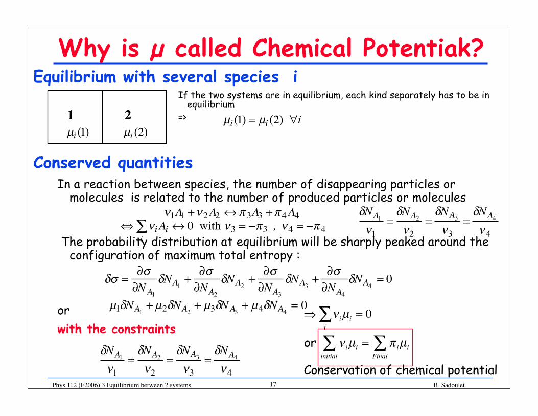
Why is µ called Chemical Potentiak?Equilibrium with several species i

If the two systems are in equilibrium, each kind separately has to be in equilibrium

=>

Conserved quantitiesIn a reaction between species, the number of disappearing particles or

molecules is related to the number of produced particles or molecules

The probability distribution at equilibrium will be sharply peaked around the configuration of maximum total entropy :

orwith the constraints

µi 1( ) = µi 2( ) ∀i21µi 1( ) µi 2( )

ν1A1 +ν2A2 ↔π 3A3 +π 4A4⇔ νi Ai

i∑ ↔ 0 with ν3 = −π3 , ν4 = −π 4

δσ =∂σ∂NA1

δNA1 +∂σ∂NA2

δNA2 +∂σ∂NA3

δNA3 +∂σ∂NA4

δNA4 = 0

µ1δNA1 + µ2δNA2 + µ3δNA3 + µ4δNA4 = 0

δNA1ν1

=δNA2ν2

=δNA3ν3

=δNA4ν4

δNA1ν1

=δNA2ν2

=δNA3ν3

=δNA4ν4

⇒ ν iµii∑ = 0

or ν iµiinitial∑ = π iµi

Final∑

Conservation of chemical potential

Phys 112 (F2006) 3 Equilibrium between 2 systems B. Sadoulet18

Law of mass actionLaw of Mass Action

Consider the reaction

or

=>

or

νiAii∑ ↔ 0

ν iµi

i∑ = 0 with µi = τ log

ninQi

⎛

⎝⎜⎞

⎠⎟ninQi

⎛

⎝⎜⎞

⎠⎟i∏

νi

= 1

niνi

i∏ = K τ( ) with K τ( ) = nQi( )

i∏ νi

niνi

initial i∏

njπ j

final j∏

= K τ( ) with K τ( ) =nQi( )νi

initial i∏

nQj( )π j

final j∏