Microbial Dose-Response Curves and Disinfection EfficacyModels Revisited

Micha Peleg1

Received: 25 June 2020 /Accepted: 7 August 2020# Springer Science+Business Media, LLC, part of Springer Nature 2020

AbstractThe same term “dose-response curve” describes the relationship between the number of ingested microbes or their logarithm, and theprobability of acute illness or death (type I), and between a disinfectant’s dose and the targeted microbe’s survival ratio (type II), akinto survival curves in thermal and non-thermal inactivation kinetics. The most common model of type I curves is the cumulative formof the beta-Poisson distribution which is sometimes indistinguishable from the lognormal or Weibull distribution. The most notablesurvival kinetics models in static disinfection are of the Chick-Watson-Hom’s kind. Their published dynamic versions, however,should be viewed with caution. Amicrobe population’s type II dose-response curve, static and dynamic, can be viewed as expressingan underlying spectrum of individual vulnerabilities (or resistances) to the particular disinfectant. Therefore, such a curve can bedescribed mathematically by the flexible Weibull distribution, whose scale parameter is a function of the disinfectant’s intensity,temperature, and other factors. But where the survival ratio’s drop is so steep that the static dose-response curve resembles a stepfunction, the Fermi distribution function becomes a suitable substitute. The utility of the CT (or Ct) concept primarily used in waterdisinfection is challenged on theoretical grounds and its limitations highlighted. It is suggested that stochastic models of microbialinactivation could be used to link the fates of individual viruses or bacteria to their manifestation in the survival curve’s shape.Although the emphasis is on viruses and bacteria, most of the discussion is relevant to fungi, protozoa, and perhaps worms too.

Keywords Kinetics .Viruses .Bacteria . CT (orCt) . Chick-Watson-Hom’smodels .Distribution functions . Stochasticmodels .

Survival models

Introduction

COVID 19 [43, 45] transmission through consumption ofcontaminated food has not been an issue in the current crisis,but other kinds of viruses remain a health hazard [3, 10, 52].Conventional food preservation methods, primarily targetingcellular organisms especially bacteria, have been apparentlyefficient in destroying viruses as well [4]. However, meat-processing plants have recently emerged as hotspots in thepandemic spread in rural areas, and food service operationsbeen identified as potential culprits of its spread amonghumans. Thus, not surprisingly, disinfection of personnel, pro-duce, clothing, air, tools, equipment, or any surface thathumans can be in contact with has recently become a commonpractice and increasingly mandated by health authorities.

There is a very rich body of scientific and technical litera-ture on disinfection. Being an integral part of medicine, water,and air purification, and an important aspect of the food, phar-maceutical, and other industries, the various aspects of disin-fection, including its kinetics, have been extensively investi-gated at every relevant level form the molecular to theepidemiological.

The objective of this review is neither to evaluate andcompare the efficacy of the various available disinfectionmethods and explain their underlying biological/chemical/biochemical/physical principles, nor to discuss the engi-neering aspects of their implementation. This work hasthe very limited scope to highlight and assess the theoret-ical implications of the similarities and dissimilarities be-tween kinetic models of water, air and surface disinfection,and those used to quantify the efficacy of food preserva-tion methods, thermal and non-thermal. Although specialattention will be given to viruses and bacteria, we shouldalways keep in mind that most of the technologies andagents used for their disinfection are also effective againstother biological contaminants.

* Micha Pelegmicha.peleg@foodsci.umass.edu

1 Department of Food Science, University of Massachusetts,Amherst, MA 01003, USA

https://doi.org/10.1007/s12393-020-09249-6

/ Published online: 28 August 2020

Food Engineering Reviews (2021) 13:305–321

Terms and Definitions

Disinfection, according to the Centers for Disease Control andPrevention (CDC), is a “process that eliminates many or allpathogenic microorganisms, except bacterial spores, on inan-imate objects.” It differs from sterilization, which “eliminatesall forms of microbial life” and from cleaning (also calledsanitation) which is “the removal of visible soil (e.g., organicand inorganic material) from objects and surfaces and normal-ly is accomplishedmanually or mechanically using water withdetergents or enzymatic products.”

Disinfectants, according to Wikipedia, are “chemicalagents designed to inactivate or destroy microorganisms oninert surfaces,”which may include fresh produce [26]. But theterm also applies to chemical agents used to disinfect waterand air [1, 17, 21, 43, 44, 46, 49], ultraviolet (UV) light [23],other forms of radiation [14, 15], and even cold plasma [31].

Dose in our context can be defined as the quantity of dis-infectant used in a particular application. Originally, it referredto an amount of medicine prescribed to (dosis in Greek) or ofingested poison by a human. Now, the term is also used for theamount of disinfectant administered to a targeted microorgan-ism or the medium in which it may reside or the surface onwhich it may be present (see below).

Dose-response curve (or exposure-response relationship)according to Wikipedia “describes the magnitude of the re-sponse of an organism, as a function of exposure to a stimulusor stressor after a certain exposure time.” The response iscommonly expressed as the percent of inactivated organismsand hence has the range of 0 to 100% (see below).

LD50 is the median lethal dose, i.e., the dose that corre-sponds to a response of 50% inactivation. It is used to comparedisinfectants’ potency; the lower the LD50 the higher is theagent toxicity or treatment efficacy.

Survival curve in our context is a plot of the number orfraction of surviving organisms (or viable viruses) or its log-arithm (almost always 10 based) as a function of the expo-sure’s time, commonly expressed in seconds, minutes orhours. A survival curve obtained under constant lethal agent’sintensity and environmental conditions is referred to as static.A survival curve obtained under varying lethal agent’s inten-sity and environmental conditions is referred to as dynamic(see below). Notice that in both static and dynamic exposuresto a lethal agent, the survival curve’s local slope, which hastime reciprocal units, is the momentary (“instant”) inactivationrate and hence the connection to kinetics [35].

Issues with the Definition of a Dose

Ostensibly, the above-listed definitions are all straightforwardand their meanings intuitively clear. Yet, this is not always thecase with the dose definition, which is a core issue whentrying to relate the dose-response curve to the inactivation

kinetics. Here is why caution is needed. When dealing withthe potency or toxicity of a drug, poison, or any substanceingested by a human or animal, a dose can be quantified interms and units such asmg ingested/kg of the ingesting personor animal. Similarly, the number of a pathogenic microorgan-ism’s cells or virus’s units ingested by an individual humancan also be viewed as a dose. Indeed, a pathogen’s virulenceand infectivity, which determine the severity of the damagethat it causes and the speed of its spread, are intimately asso-ciated with the number of ingested cells or virus units neededfor acute infection. In contrast, in water or air disinfection, thedisinfectant’s effective concentration is determined in themedium where the targeted pathogen resides and not in themicroorganism or virus itself. Similarly, in surface disinfec-tion by an active chemical compound or radiation, the treat-ment’s intensity is expressed in terms of mass or energy perunit treated area and not per the targeted individual microbe’scell or virus unit, or a specified number of the targeted cells orunits, or even their biomass, which would depend on the con-tamination level and its pattern.

Moreover, rarely is the desired disinfection level goal,expressed as the number of decades reduction in the targetedmicrobial population’s size, is accomplished instantaneously.Consequently, the exposure’s duration becomes a crucial con-sideration and ought to be taken into account in the treatment’sintensity quantification. This is manifested in the CT, or Ct,concept [32] according to which a chemical disinfectant’ ef-fective dose is expressed as the multiplication product of thedisinfectant’s concentration (C) and the exposure time (T or t)needed to reduce the targeted microbial population’s by achosen number of decades, an issue to which we will return.(The confusing traditional CT term, where T represents timeand not temperature (and which has nothing to do with theState of Connecticut…), is a carry on from an older publica-tion where the integration limit of t was assigned the letter T.)

Also, in chemical disinfection processes, the administeredlethal agent is a highly active chemical compound, e.g., ozone,chlorine dioxide, or paracetic acid. Such compounds arechemically unstable; the primary cause of their reactivity andrationale of their use as disinfectants. But as a result, theireffective concentration diminishes with time, sometimes re-quiring their constant or periodical replenishment. The gas-eous disinfectants are also volatile and hence, their effectiveconcentration can diminish even without chemicallydisintegrating or reacting with the targeted microbe. Eitherway, maintaining a predetermined constant concentration ofsuch chemical agents during the disinfection process, or evenin studies of its kinetics in the laboratory, is technically diffi-cult. This makes the experimental determination of perfectlystatic survival curves, and similarly dose-response curves, achallenging task. It also raises the question of whether theinitial or average concentration is or can be an acceptablerepresentative of the diminishing effective concentration.

306 Food Eng Rev (2021) 13:305–321

The above issues, especially how to account for the time’s rolein disinfection mathematically, have been and can be tackledin various ways, which we’ll address in what follows. Sufficeit to state at this point is that since time is inherently involvedin both dose-response and survival curves, each cannot beconsidered in isolation but as a manifestation of the sameunderlying inactivation kinetics.

Viral Versus Bacterial Inactivation

There is an ongoing debate on whether a virus can be consid-ered a life form but it should not concern us here. From amathematical modeling viewpoint, the inactivation of a viral,bacterial, or other microbial population follows similar kinet-ics despite that the underlying mechanisms at the individualcell/unit and molecular levels can be quite different. Since inwhat follows, we’ll only address the kinetics at the populationlevel, the focus will be on concepts and models that are perti-nent to the disinfection of either or both viruses and bacteria.

There are two main differences between viral and otherorganismic populations that should be always kept in mind:

1. Unlike at least certain kinds of bacteria, viruses do nothave damage repair mechanisms. Therefore, unless prov-en otherwise, their inactivation can be viewed as irrevers-ible. It will be assumed, however, as has presumably beendone in the cited publications, that the same applies tobacteria and other pathogens on the pertinent time scale.In other words, we will assume that issues concerninginjury, repair, and/or adaptation need not be taken intoaccount for modeling the disinfection kinetics.

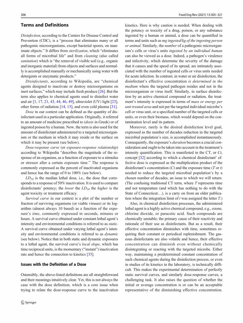
2. Unlike in a decimated bacterial and other microbial pop-ulation, the number of survivors in a viral population, ifany, cannot rise without recontamination. In other words,depending on conditions, the survivors of a bacterial orother microbial population can resume cell division. Thus,at least in principle, their numbers can not only rise butalso exceed the original contamination level. This demon-strated in Fig. 1. It shows the screen display of a freelydownloadable Wolfram Demonstration that can be usedto simulate such and other inactivation/growth scenarios(open : h t tps : / /demons t r a t ions .wol f r am.com/GrowthInhibitionAndRetardationByAntimicrobials/).[To run the Demonstration and download, the also freelydownloadable Wolfram CDF Player, which runs it andmore than 12,000 other Demonstrations to date, followinstructions on the screen.] We will also assume that forthe time scale pertinent to disinfection the issue of sporegermination need not be addressed.

There can also be differences between how long viruses,bacteria, and other microorganisms remain viable when

dispersed in untreated air or water, or on a contaminated sur-face. These differences can vary dramatically depending onthe virus or organism type, the particular habitat, and on theambient conditions, notably temperature, and in air or on asurface on the relative humidity too. It has been traditionallyassumed though that the rate of a pathogen perishing sponta-neously is very small relative to that induced by a disinfectant,and therefore need not be taken into account in dose-responseor survival curves modeling. Nevertheless, although true, wewill still show how natural attrition can be incorporated into asurvival model if needed.

Dose-Response Models

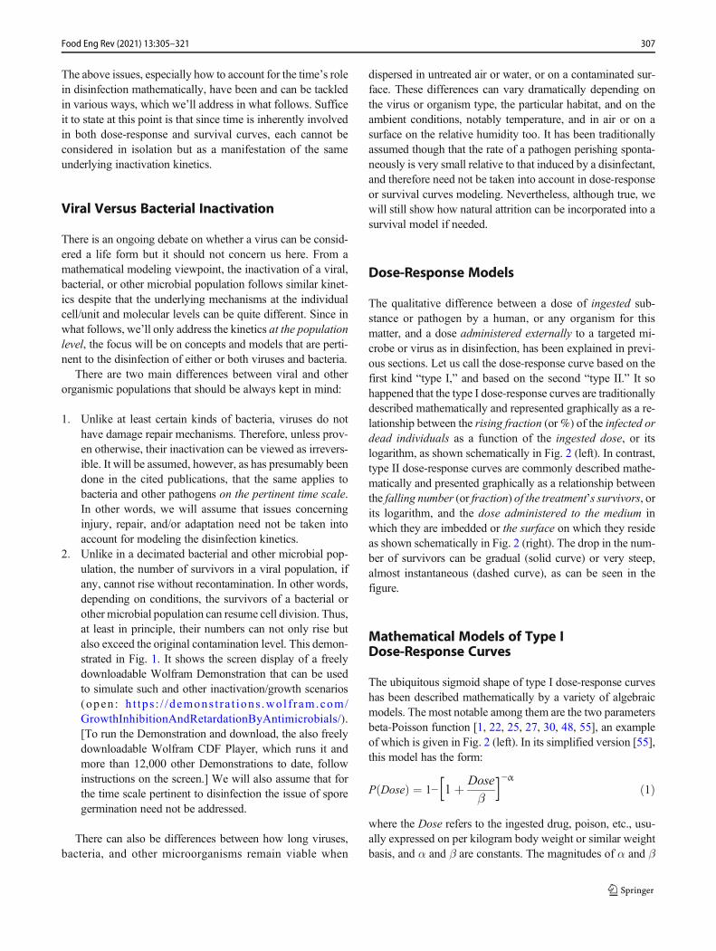
The qualitative difference between a dose of ingested sub-stance or pathogen by a human, or any organism for thismatter, and a dose administered externally to a targeted mi-crobe or virus as in disinfection, has been explained in previ-ous sections. Let us call the dose-response curve based on thefirst kind “type I,” and based on the second “type II.” It sohappened that the type I dose-response curves are traditionallydescribed mathematically and represented graphically as a re-lationship between the rising fraction (or %) of the infected ordead individuals as a function of the ingested dose, or itslogarithm, as shown schematically in Fig. 2 (left). In contrast,type II dose-response curves are commonly described mathe-matically and presented graphically as a relationship betweenthe falling number (or fraction) of the treatment’s survivors, orits logarithm, and the dose administered to the medium inwhich they are imbedded or the surface on which they resideas shown schematically in Fig. 2 (right). The drop in the num-ber of survivors can be gradual (solid curve) or very steep,almost instantaneous (dashed curve), as can be seen in thefigure.

Mathematical Models of Type IDose-Response Curves

The ubiquitous sigmoid shape of type I dose-response curveshas been described mathematically by a variety of algebraicmodels. The most notable among them are the two parametersbeta-Poisson function [1, 22, 25, 27, 30, 48, 55], an exampleof which is given in Fig. 2 (left). In its simplified version [55],this model has the form:

P Doseð Þ ¼ 1−½1þ Doseβ�−α ð1Þ

where the Dose refers to the ingested drug, poison, etc., usu-ally expressed on per kilogram body weight or similar weightbasis, and α and β are constants. The magnitudes of α and β

307Food Eng Rev (2021) 13:305–321

depend on the toxicmaterial kind and the manner in which it isingested. According to this model LD50 = β/(21/α − 1).

The lethal or infectious Dose can also be the number N ofingested, inhaled, or injected virus units or a pathogenic bac-terium’s cells in which case the model will assume the form:

P Nð Þ ¼ 1− 1þ NβN

� �−αN

ð2Þ

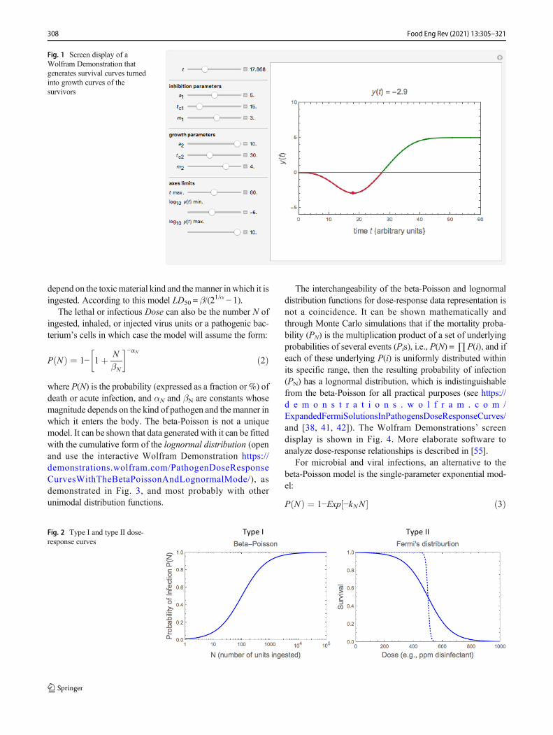
where P(N) is the probability (expressed as a fraction or %) ofdeath or acute infection, and αN and βN are constants whosemagnitude depends on the kind of pathogen and the manner inwhich it enters the body. The beta-Poisson is not a uniquemodel. It can be shown that data generated with it can be fittedwith the cumulative form of the lognormal distribution (openand use the interactive Wolfram Demonstration https://demonstrations.wolfram.com/PathogenDoseResponseCurvesWithTheBetaPoissonAndLognormalMode/), asdemonstrated in Fig. 3, and most probably with otherunimodal distribution functions.

The interchangeability of the beta-Poisson and lognormaldistribution functions for dose-response data representation isnot a coincidence. It can be shown mathematically andthrough Monte Carlo simulations that if the mortality proba-bility (PN) is the multiplication product of a set of underlyingprobabilities of several events (Pis), i.e., P(N) = ∏ P(i), and ifeach of these underlying P(i) is uniformly distributed withinits specific range, then the resulting probability of infection(PN) has a lognormal distribution, which is indistinguishablefrom the beta-Poisson for all practical purposes (see https://d e m o n s t r a t i o n s . w o l f r a m . c o m /ExpandedFermiSolutionsInPathogensDoseResponseCurves/and [38, 41, 42]). The Wolfram Demonstrations’ screendisplay is shown in Fig. 4. More elaborate software toanalyze dose-response relationships is described in [55].

For microbial and viral infections, an alternative to thebeta-Poisson model is the single-parameter exponential mod-el:

P Nð Þ ¼ 1−Exp −kNN½ � ð3Þ

Fig. 1 Screen display of aWolfram Demonstration thatgenerates survival curves turnedinto growth curves of thesurvivors

Type I Type IIFig. 2 Type I and type II dose-response curves

308 Food Eng Rev (2021) 13:305–321

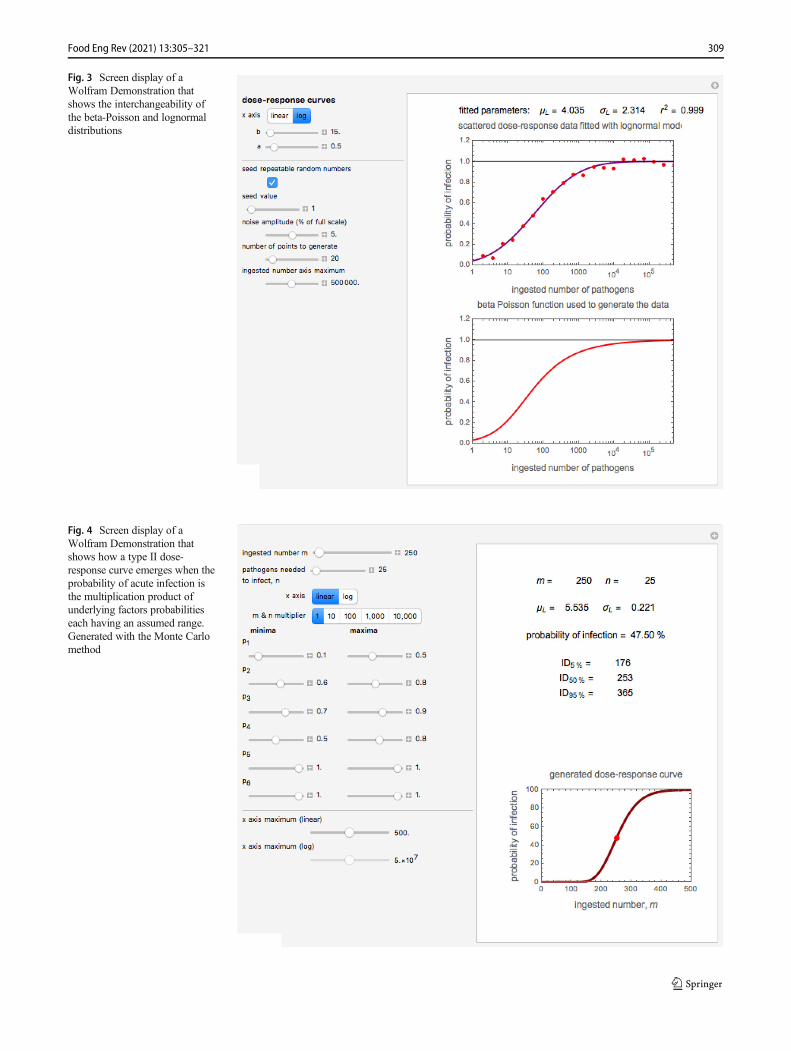
Fig. 3 Screen display of aWolfram Demonstration thatshows the interchangeability ofthe beta-Poisson and lognormaldistributions

Fig. 4 Screen display of aWolfram Demonstration thatshows how a type II dose-response curve emerges when theprobability of acute infection isthe multiplication product ofunderlying factors probabilitieseach having an assumed range.Generated with the Monte Carlomethod

309Food Eng Rev (2021) 13:305–321

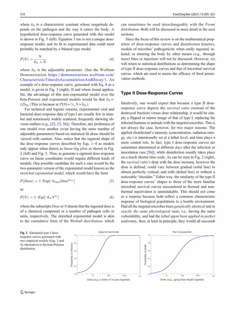
where kN is a characteristic constant whose magnitude de-pends on the pathogen and the way it enters the body. Ahypothetical dose-response curve generated with this modelis shown in Fig. 5 (left). Equation 3 too is not a unique dose-response model, and its fit to experimental data could mostprobably be matched by a Monod type model

P Nð Þ ¼ NbN þ N

ð4Þ

where bN is the adjustable parameter. (See the WolframDemonstration https://demonstrations.wolfram.com/CharacteristicTimesInAccumulationAndDecay/). Anexample of a dose-response curve, generated with Eq. 4 as amodel, is given in Fig. 5 (right). If and where found applica-ble, the advantage of this non-exponential model over thebeta-Poisson and exponential models would be that bN =LD50. (This is because at P(N) = ½, N = bN.)

For technical and logistic reasons, experimental viral andbacterial dose-response data of type I are usually few in num-ber and notoriously widely scattered, frequently showing ob-vious outliers (e.g., [22, 53, 56]). Therefore, any preference ofone model over another (even having the same number ofadjustable parameters) based on statistical fit alone should beviewed with caution. Also, notice that the sigmoid shape ofthe dose-response curves described by Eqs. 1–4 as modelsonly appear when drawn as linear-log plots as shown in Fig.2 (left) and Fig. 5. Thus, to generate a sigmoid dose-responsecurve on linear coordinates would require different kinds ofmodels. One possible candidate for such a case would be thetwo-parameter version of the exponential model known as thestretched exponential model, which would have the form

P Doseð Þ ¼ 1−Exp −kDoseDosenDose½ � ð5Þor

P Nð Þ ¼ 1−Exp −kNNnN½ � ð6Þ

where the subscriptsDose orN denote that the ingested dose isof a chemical compound or a number of pathogen cells orunits, respectively. The stretched exponential model is akinto the cumulative form of the Weibull distribution, which

can sometimes be used interchangeably with the Fermidistribution. Both will be discussed in more detail in the nextsections.

Since the focus of this review is on the mathematical prop-erties of dose-response curves and disinfection kinetics,models of microbes’ pathogenicity when orally ingested, in-haled, or entering the body by other means (e.g., throughinsect bites or injection) will not be discussed. However, wewill return to statistical distributions as determining the shapeof type II dose-response curves and that of microbial survivalcurves, which are used to assess the efficacy of food preser-vation methods.

Type II Dose-Response Curves

Intuitively, one would expect that because a type II dose-response curve depicts the survival ratio (instead of thedestroyed fraction) versus dose relationship, it would be sim-ply a flipped or mirror image of that of type I, replacing theinfected humans or animals with the targeted microbes. This isnot always the case, however, for two major reasons: Theapplied disinfectant’s intensity (concentration, radiation ener-gy, etc.) is intentionally set at a lethal level, and time plays amore central role. In fact, type I dose-response curves aresometimes determined at different days after the infection orinoculation (see [56]), while disinfection usually takes placeon a much shorter time scale. As can be seen in Fig. 2 (right),the survival ratio’s drop with the dose increase, however thedose is defined, could vary between gradual (solid line) toalmost perfectly vertical, and with (dotted line) or without anoticeable “shoulder.” Either way, the similarity of the type IIdose-response curves’ shapes to those of the more familiarmicrobial survival curves encountered in thermal and non-thermal inactivation is unmistakable. This should not comeas a surprise because both reflect a common characteristicresponse of biological populations to a hostile environment.Had all the targeted microbes been genetically identical and inexactly the same physiological state, i.e., having the samevulnerability, and had the lethal agent been applied in perfectuniformity, then, at least in principle, they would all succumb

Fig. 5 Simulated type I dose-response curves generated withtwo empirical models (Eqs. 3 and4), alternatives to the beta-Poissondistribution

310 Food Eng Rev (2021) 13:305–321

to the very same dose at exactly the same time. The dose-response curve in such a case would be a perfect step function[33–35] very similar to that shown as a dotted curve in Fig. 2(right). The corresponding dose magnitude in such a casewould be a measure of the individual virus unit or bacterialcell’s sensitivity to or tolerance of the lethal agent, which allmembers of the population share and exhibit in unison, or viceversa. A dose-response curve having the shape of a perfectstep function would indicate that the above-mentioned condi-tions are fully satisfied; i.e., that all the targeted viruses orbacterial cells are indeed identical and they succumb simulta-neously to the uniformly applied disinfectant. Obviously, thisis rarely the case in practice and most type II dose-responsecurves indicate that there is an underlying narrow or widespectrum of sensitivities and/or at least a certain degree ofnon-uniformity in the exposure’s intensity [39]. Let us empha-size that for a true step dose-response curve to appear, bothuniformity conditions ought to be satisfied simultaneously.But viruses can at least sometimes exhibit slight composition-al variations [47, 48] and their dispersion pattern might not beuniform due to aggregation, for example [5, 29]. Residing on anon-uniform surface may also cause non-uniform exposure.Bacteria and other microorganisms, even if their dispersion isuniform can be in different physiological states as a result ofage, cell division stage, etc. Consequently, type II dose-response curves closely resembling a step function are uncom-mon [33–35]. The concept of an underlying spectrum of sen-sitivities or resistances also applies to the various shapes ofsurvival curves (see below) except that their primary manifes-tation is in the survival ratio’s dependence on time.

Prominent Flat Shoulder

A prominent flat shoulder in a type II dose-response curves (ofthe kind shown in Fig. 2 (right)) has been reported in variouspublications (e.g., [8, 32]). The shoulder’s presence has beencommonly considered a special case where the drop in thesurvival ratio commences only after the administration of acritical dose or as a consequence of a characteristic physiolog-ical lag time. In other words, the idea has been that there aretwo distinct response regimes and a sharp transition betweenthem. An alternative view is that both type II dose-responsecurves (of the kind shown in Fig. 2 (right)) and survival curvesencountered in thermal food preservation having a similarshape are actually the cumulative form of an underlyingunimodal distribution of the targeted microbe’s sensitivitiesto the imposed lethal agent. The sensitivities (or resistances)are manifested in the dose needed to inactivate the microbe inthe former, or the time it takes to inactivate it in the latter.From this viewpoint, the primary difference between a dose-response and a survival curve is that in the first, the survivalratio is presented as a function of dose while in the second as afunction of time. If this observation is correct, then a

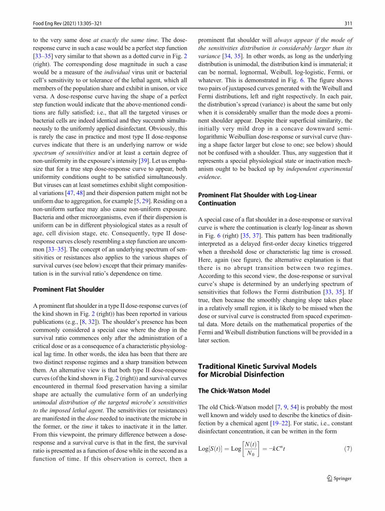
prominent flat shoulder will always appear if the mode ofthe sensitivities distribution is considerably larger than itsvariance [34, 35]. In other words, as long as the underlyingdistribution is unimodal, the distribution kind is immaterial; itcan be normal, lognormal, Weibull, log-logistic, Fermi, orwhatever. This is demonstrated in Fig. 6. The figure showstwo pairs of juxtaposed curves generated with theWeibull andFermi distributions, left and right respectively. In each pair,the distribution’s spread (variance) is about the same but onlywhen it is considerably smaller than the mode does a promi-nent shoulder appear. Despite their superficial similarity, theinitially very mild drop in a concave downward semi-logarithmic Weibullian dose-response or survival curve (hav-ing a shape factor larger but close to one; see below) shouldnot be confused with a shoulder. Thus, any suggestion that itrepresents a special physiological state or inactivation mech-anism ought to be backed up by independent experimentalevidence.

Prominent Flat Shoulder with Log-LinearContinuation

A special case of a flat shoulder in a dose-response or survivalcurve is where the continuation is clearly log-linear as shownin Fig. 6 (right) [35, 37]. This pattern has been traditionallyinterpreted as a delayed first-order decay kinetics triggeredwhen a threshold dose or characteristic lag time is crossed.Here, again (see figure), the alternative explanation is thatthere is no abrupt transition between two regimes.According to this second view, the dose-response or survivalcurve’s shape is determined by an underlying spectrum ofsensitivities that follows the Fermi distribution [33, 35]. Iftrue, then because the smoothly changing slope takes placein a relatively small region, it is likely to be missed when thedose or survival curve is constructed from spaced experimen-tal data. More details on the mathematical properties of theFermi andWeibull distribution functions will be provided in alater section.

Traditional Kinetic Survival Modelsfor Microbial Disinfection

The Chick-Watson Model

The old Chick-Watson model [7, 9, 54] is probably the mostwell known and widely used to describe the kinetics of disin-fection by a chemical agent [19–22]. For static, i.e., constantdisinfectant concentration, it can be written in the form

Log S tð Þ½ � ¼ LogN tð ÞN0

� �¼ −kCnt ð7Þ

311Food Eng Rev (2021) 13:305–321

where S(t) is the survival ratio, defined as N(t), the number ofviable survivors after time t, divided by N0, the initial numberof the targeted virus units or microbial cells, and C is the“residual disinfectant concentration.” The model’s two adjust-able parameters, k and n, are characteristic to the targetedmicrobe and the particular disinfectant. Their magnitudes de-pend on the type of mediumwhere the disinfection takes placeand ambient conditions, notably temperature and pH, or rela-tive humidity where relevant. Whether Log[S(t)]’s base is e or10 is immaterial and will be only manifested in the numericalvalue of the corresponding k.

The rate version of the Chick-Watson model according tothe literature [19, 32] has the form

dN tð Þdt

¼ −kCnt ð8Þ

From a formal viewpoint, Eq. 8 describes a static first-orderdecay or loss kinetics where the characteristic rate constant k,in time reciprocal units, is proportional to the momentary dis-infectant’s concentration raised to the power n, i.e., k = kCn.To avoid confusion, let it be understood that Eq. 8 in the aboveform only applies to a constant disinfectant concentration, orin other words, it can only describe the targeted microbe’sdecay rate if and only if the disinfectant concentration remainsunchanged during the disinfection (see below).

Hom’s Model

An expanded version of the Chick-Watson survival model isknown as Hom’s model, which for static disinfection can bewritten in the form [21].

Log S tð Þ½ � ¼ LogN tð ÞN0

� �¼ −kCntm ð9Þ

where the three parameters are k and n transplanted from theChick-Watson model, and m an added exponent. The originalChick-Watson equation is therefore a special case of theHom’s model where m = 1.

According to various publications (e.g., [18–20]), Hom’smodel underlying differential rate equation is

dN tð Þdt

¼ −kmCntm−1N tð Þ ð10Þ

Although apparently intended to describe dynamic disin-fection, the above form of Hom’s model, like its predecessorEq. 8, is only applicable to processes where the disinfectantconcentration remains constant throughout the entire disinfec-tion process. In other words, Eq. 10 can describe the targetedmicrobe’s elimination rate if and only if the disinfectant’sconcentration and hence the term Cn is not a function of time.If, however, the residual disinfectant concentration falls, rises(through replenishment) and/or oscillates, that is varied andbecomes a function of time, i.e., C =C(t) ≠ constant, then thegoverning differential rate equation ought to be

dLog S tð Þ½ �dt

¼ −ktm−1C tð Þn−1 mC tð Þ þ ntdC tð Þdt

� �ð11Þ

where the actual time t is the same as the time t* (see below),which corresponds to the momentary survival ratio, i.e., the(numerical) solution for t of the equation

Log S tð Þ½ � ¼ −k*C tð Þntm ð12Þ

Fig. 6 “Long flat shoulder” in thecumulative form of unimodaldistributions when their mode ismuch larger than their variance

312 Food Eng Rev (2021) 13:305–321

(For details see [13, 35] and below.)Despite its cumbersome appearance, Eq. 11, especially

with t* being a momentary numerical solution of an algebraicequation, is still an ordinary differential equation (ODE).Thus, although yet be attempted, one can expect that withmodern mathematical software Eq. 11 would be solved nu-merically for almost any conceivable concentration profileC(t) expressed algebraically. At least in principle, if and whenthe Chick-Watson or Hom’s model is validated experimental-ly, Eq. 11 could be used to simulate or predict the outcome ofrealistic actual or contemplated dynamic disinfection process-es, where the disinfectant concentration does vary with time.

The reported applicability of the Chic-Watson-Hom’smodels, in their original and modified versions, seems to havebeen primarily based on their respective equations’ fit to ex-perimental static data, rather than to their ability to predictdynamic survival patterns. Unfortunately, good fit by statisti-cal criteria alone cannot be considered a model validation. Thefit only provides evidence that the proposed model candescribe the observed data at hand mathematically and doesnot even establish its uniqueness. Proper validation of a sur-vival model, or of any kinetic model for that matter, requiresthat it can predict correctly survival data not used in its pa-rameters determination, for example, predicting correctly dy-namic survival curves from static data or vice versa, or dy-namic survival data from other dynamic survival data [13, 35,37].

Models Based on an Underlying Spectrumof Sensitivities

Alternatives to the Chick-Watson-Holm’s type survivalmodels are the already mentioned models based on an under-lying spectrum of sensitivities or resistances described by adistribution function. Several such distribution functions canbe considered. The first two natural candidates that come tomind are the commonplace and highly flexible Weibull andlognormal distributions, or for the less common case of anextremely narrow distribution, where the dose-response orsurvival curve resembles a step function, the less familiarFermi distribution becomes a promising option [33], as dem-onstrated in Fig. 2.

The Weibull Distribution

The Weibull distribution has been used in the mathematicaldescription of a wide range of failure phenomena and hence itsubiquitous association with risk assessment in a variety oftechnological fields. Since the inactivation or death of an in-dividual microbe during disinfection can be viewed as its fail-ure to overcome the destructive or lethal agent, the Weibull

distribution is a natural choice [13, 35]. The two parameters ofthe more familiar form of the distribution function named afterWeibull are α known as the shape factor and β known as thescale factor. For our purpose, since we deal with a process’skinetics, we will use the model’s version known as the Rosin-Rammler distribution, which had been proposed (to particle-size reduction operations) 3 years prior to its introduction byWeibull [6].

For static disinfection (constant disinfectant concentration),it can be written in the form [2, 13, 35].

Log S tð Þ½ � ¼ −b Cð Þtm Cð Þ ð13Þwhere b(C) is a concentration-dependent rate parameter, relat-ed to Weibull’s scale factor reciprocal, and m(C) a power thatcan but need not be concentration-dependent, equivalent toWeibull’s shape factor. Where and when m(C) is independentor practically independent of the concentration, which is notuncommon (see [49, 50, 51]), the static model becomes

Log S tð Þ½ � ¼ −b Cð Þtm ð14Þ

This equation is reminiscent of Hom’s model, except thatthe rate parameter b(C) need not be in the form of the power-law expression. In other words, Hom’s model can be viewedas a special case of the Weibullian model where b(C) = kCn.

Implementing the assumption that in dynamic disinfection,where C =C(t), not a constant, the momentary inactivationrate is the static rate at the disinfectant’s momentary concen-tration, at the time that corresponds to the momentary surviv-al ratio [13, 35], renders the rate model

dLog S tð Þ½ �dt

¼ −b C tð Þ½ �m −Log S tð Þ½ �bhC tð Þ

i24

35

m−1ð Þ=m

ð15Þ

Here, again, despite its cumbersome appearance, Eq. 15 isstill an ordinary differential equation (ODE). Therefore, as hasbeen already demonstrated [ibid], it can be rapidly solvednumerically with modern mathematical software for almostany conceivable relevant concentration history C(t) expressedalgebraically, including containing If statements to accountfor instant replenishments. Thus, at least in principle, thismodel can replace the Chick-Watson-Hom type models whenvalidated experimentally by testing its predictive ability.Examples of Eq. 15’s solutions for disinfection with a dissi-pating agent can be generated with a freely downloadableinteractive Wolfram Demonstration https://demonstrations.w o l f r a m . c o m /MicrobialSurvivalWithDissipatingDisinfectant/. Its screendisplay is shown in Fig. 7.

According to the Weibullian model [35], if the shape fac-tor, i.e., the power m, is larger than one (m > 1), the staticsurvival curve has downward concavity, which suggests that

313Food Eng Rev (2021) 13:305–321

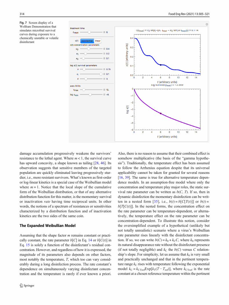
damage accumulation progressively weakens the survivors’resistance to the lethal agent. Where m < 1, the survival curvehas upward concavity, a shape known as tailing [28, 46]. Itsobservation suggests that sensitive members of the targetedpopulation are quickly eliminated leaving progressively stur-dier, i.e., more resistant survivors.What’s known as first-orderor log-linear kinetics is a special case of the Weibullian modelwhere m = 1. Notice that the local slope of the cumulativeform of the Weibullian distribution, or that of any alternativedistribution function for this matter, is the momentary survivalor inactivation rate having time reciprocal units. In otherwords, the notions of a spectrum of resistances or sensitivitiescharacterized by a distribution function and of inactivationkinetics are the two sides of the same coin.

The Expanded Weibullian Model

Assuming that the shape factor m remains constant or practi-cally constant, the rate parameter b[C] in Eq. 14 or b[C(t)] inEq. 15 is solely a function of the disinfectant’s residual con-centration. However, and regardless of how it is expressed, themagnitude of its parameters also depends on other factors,most notably the temperature, T, which too can vary consid-erably during a long disinfection process. The rate constant’sdependence on simultaneously varying disinfectant concen-tration and the temperature is rarely if ever known a priori.

Also, there is no reason to assume that their combined effect issomehow multiplicative (the basis of the “gamma hypothe-sis”). Traditionally, the temperature effect has been assumedto follow the Arrhenius equation despite that its universalapplicability cannot be taken for granted for several reasons[16, 39]. The same is true for alternative temperature depen-dence models. In an assumption-free model where only theconcentration and temperature play major roles, the static sur-vival rate parameter can be written as b(C, T). If so, then indynamic disinfection the momentary disinfection can be writ-ten in a nested form [35], i.e., b(t) = b[C[T(t)]] or b(t) =b[T[C(t)]]. In the nested forms, the concentration effect onthe rate parameter can be temperature-dependent, or alterna-tively, the temperature effect on the rate parameter can beconcentration-dependent. To illustrate this notion, considerthe oversimplified example of a hypothetical (unlikely butnot totally unrealistic) scenario where a virus’s Weibullianrate parameter rises linearly with the disinfectant concentra-tion. If so, we can write b(C) = k0 + kCC, where k0 representsits natural disappearance rate without the disinfectant presence(if not totally negligible) and kC the b(C) versus C relation-ship’s slope. For simplicity, let us assume that k0 is very smalland practically unchanged and that in the pertinent tempera-ture range kC rises with temperature following the exponentialmodel kC = kCTrefExp[kT(T − Tref)], where kCTref is the rateconstant at a chosen reference temperature within the pertinent

Fig. 7 Screen display of aWolfram Demonstration thatsimulates microbial survivalcurves during exposure to achemically unstable or volatiledisinfectant

314 Food Eng Rev (2021) 13:305–321

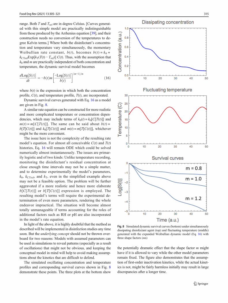
range. Both T and Tref are in degree Celsius. [Curves generat-ed with this simple model are practically indistinguishablefrom those produced by the Arrhenius equation [39], and theirconstruction needs no conversion of the temperatures to de-gree Kelvin terms.] Where both the disinfectant’s concentra-tion and temperature vary simultaneously, the momentaryWeibullian rate constant, b(t), becomes b(t) = k0 +kCTrefExp[kT(T(t) − Tref)] C(t). Thus, with the assumption thatk0 andm are practically independent of both concentration andtemperature, the dynamic survival model becomes

dLog S tð Þ½ �dt

¼ −b tð Þm −Log S tð Þ½ �b tð Þ

� � m−1ð Þ=mð16Þ

where b(t) is the expression in which both the concentrationprofile, C(t), and temperature profile, T(t), are incorporated.

Dynamic survival curves generated with Eq. 16 as a modelare given in Fig. 8.

A similar rate equation can be constructed for more realisticand more complicated temperature or concentration depen-dencies, which may include terms of k0(t) = k0[C[T(t)]] andm(t) = m[C[T(t)]]. The same can be said about b(t) =b[T[C(t)]] and k0[T[C(t)]] and m(t) =m[T[C(t)]], whichevermight be the more convenient.

The issue here is not the complexity of the resulting ratemodel’s equation. For almost all conceivable C(t) and T(t)histories, Eq. 16 will remain ODE which could be solvednumerically almost instantaneously. The issues are primar-ily logistic and of two kinds: Unlike temperature recording,monitoring the disinfectant’s residual concentration atclose enough time intervals may not be a simple matter,and to determine experimentally the model’s parameters,k0, kCTref, and kT, even in the simplified example abovemay not be a feasible option. The problem will be furtheraggravated if a more realistic and hence more elaborateb[C[T(t)]] or b[T[C(t)]] expression is employed. Theresulting model’s terms will require the experimental de-termination of even more parameters, rendering the wholeendeavor impractical. The situation will become almosttotally unmanageable if terms accounting for the roles ofadditional factors such as RH or pH are also incorporatedin the model’s rate equation.

In light of the above, it is highly doubtful that the method asdescribed will be implemented in disinfection studies any timesoon. But the underlying concept should not be thrown over-board for two reasons: Models with assumed parameters canbe used in simulations to reveal patterns (especially as a resultof oscillations) that might not be obvious, and keeping theconceptual model in mind will help to avoid making assump-tions about the kinetics that are difficult to defend.

The simulated oscillating concentration and temperatureprofiles and corresponding survival curves shown in Fig. 8demonstrate these points. The three plots at the bottom show

the potentially dramatic effect that the shape factor m mighthave if it is allowed to vary while the other model parametersremain fixed. The figure also demonstrates that the assump-tion of first-order inactivation kinetics, while the actual kinet-ics is not, might be fairly harmless initially may result in largediscrepancies after a longer time.

m = 1.0

m = 0.8

m = 1.2

Fig. 8 Simulated dynamic survival curves (bottom) under simultaneouslydissipating disinfectant agent (top) and fluctuating temperature (middle)generated with the expanded Weibullian dynamic model (Eq. 16) withthree shape factors (ms)

315Food Eng Rev (2021) 13:305–321

The Fermi Distribution

None of the already mentioned survival models can be consid-ered inherently superior and two or more of them can be fre-quently used interchangeably. The same can be said about otherunimodal distributions not mentioned. Statistical fit criteriaalone, as already stated, are insufficient to establish a model’suniqueness. A notable exception to the above is the alreadymentioned Fermi distribution function and similarly construct-ed models. They too can be indistinguishable from theWeibullor lognormal distributions when describing a wide distributionas shown in Fig. 2 (right). The Fermi model’s particular andclear advantage is its ability to describe very steep dose-response or survival curves that resemble a step function, thoseof individual microbes included. [The function was proposedby Fermi to describe the mass density distribution within anatom, which at the nucleus edge drops almost vertically toalmost zero.] When used as a dose-response or survival curvemodel it can be written in the form [33, 40].

S xð Þ ¼ 1

1þ Expx−xca

h i ð17Þ

where x is the dose (however defined) or time, xc a marker ofthe curve’s inflection point, where S(xc) = ½, and a the spreadmeasure. If a has any arbitrary value which is very small rela-tive to x − xc, then it is easy to show that Eq. 17 produces acurve that for all practical purposes looks like a step drop. Yet,the Fermi distribution function is still a continuous function thathas algebraic derivatives and can be integrated. As the value ofa increases, so does the spread around xc (the variance) andeventually, the Fermi distribution becomes almost indistin-guishable from the more familiar unimodal distribution.Notice that since

Log S xð Þ½ � ¼ −Log 1þ Expx−xca

h ih ið18Þ

then when x < < xc, Log[S(x)] ≈ 0, and when x > > xc,Log[S(x)] ≈ − (x − xc)/a as shown in Fig. 6 (right). But unlikethe 0 < x <∞ range of the Weibull or lognormal distribution,the Fermi distribution’s range is −∞ < x <∞. Consequently,S(0) is always < 1 and Log[S(0)] < 0. However, this inevitablegap is usually negligibly small and has no practical implications,especially when dealingwith highly scattered experimental data.

The CT (or Ct) Concept

According to Wikipedia: “CT Values are an important part ofcalculating disinfectant dosage for the chlorination of drinkingwater. A CT value is the product of the concentration of adisinfectant (e.g., free chlorine) and the contact time with thewater being disinfected. It is typically expressed in units of

mg-min/L.” The entry also has a table listing CT values of freechlorine (applied to Giardia cysts) in water to accomplish 1, 2,and 3 “log inactivation.”

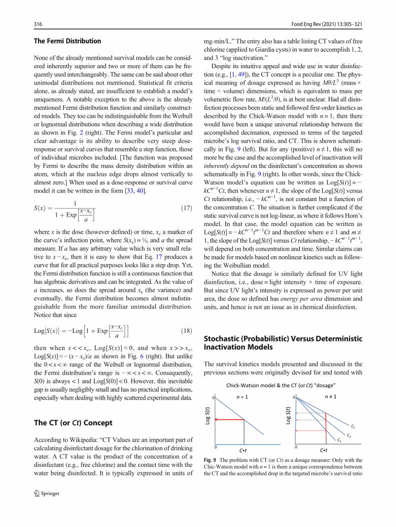
Despite its intuitive appeal and wide use in water disinfec-tion (e.g., [1, 49]), the CT concept is a peculiar one. The phys-ical meaning of dosage expressed as having Mθ/L3 (mass ×time ÷ volume) dimensions, which is equivalent to mass pervolumetric flow rate,M/(L3/θ), is at best unclear. Had all disin-fection processes been static and followed first-order kinetics asdescribed by the Chick-Watson model with n = 1, then therewould have been a unique universal relationship between theaccomplished decimation, expressed in terms of the targetedmicrobe’s log survival ratio, and CT. This is shown schemati-cally in Fig. 9 (left). But for any (positive) n ≠ 1, this will nomore be the case and the accomplished level of inactivation willinherently depend on the disinfectant’s concentration as shownschematically in Fig. 9 (right). In other words, since the Chick-Watson model’s equation can be written as Log[S(t)] = −kCn−1Ct, then whenever n ≠ 1, the slope of the Log[S(t)] versusCt relationship, i.e., − kCn−1, is not constant but a function ofthe concentration C. The situation is further complicated if thestatic survival curve is not log-linear, as where it followsHom’smodel. In that case, the model equation can be written asLog[S(t)] = − kCn−1tm−1Ct and therefore where n ≠ 1 and m ≠1, the slope of the Log[S(t)] versusCt relationship, − kCn−1tm−1,will depend on both concentration and time. Similar claims canbe made for models based on nonlinear kinetics such as follow-ing the Weibullian model.

Notice that the dosage is similarly defined for UV lightdisinfection, i.e., dose = light intensity × time of exposure.But since UV light’s intensity is expressed as power per unitarea, the dose so defined has energy per area dimension andunits, and hence is not an issue as in chemical disinfection.

Stochastic (Probabilistic) Versus DeterministicInactivation Models

The survival kinetics models presented and discussed in theprevious sections were originally devised for and tested with

n = 1

C�t

Log S(t)

C1

C�t

Log S(t)

00

Chick-Watson model & the CT (or Ct) “dosage”

0 0

n ≠ 1

C2C3

Fig. 9 The problem with CT (or Ct) as a dosage measure: Only with theChic-Watson model with n = 1 is there a unique correspondence betweenthe CT and the accomplished drop in the targeted microbe’s survival ratio

316 Food Eng Rev (2021) 13:305–321

very large microbial populations reduced through disinfectionby several orders of magnitude. They are all deterministic andexpressed in the form of cont inuous func t ions .“Deterministic” in our context is manifested in that the surviv-al curve is reproducible (despite that the individual countsthemselves can be somewhat scattered, the main reason fortheir replication) and that when presented in the form of thesurvival ratio or its logarithm versus time relationship, theinitial number is unimportant as long as there are enoughmicrobes to be counted. [There are special cases where theinitial inoculum size can be an issue but these should notconcern us here.] But the same deterministic models that areapplicable to large microbial populations may not be alwaysapplicable to very small microbial populations, especiallywhen they are subjected to a marginal disinfection treatment.This is because at the individual microbe’s level, even appar-ent continuity no more exists and probability plays a centralrole in whether it will survive or succumb after a given time.

Reports on the use of discrete stochastic (probabilistic)models of microbial inactivation are rather scarce in the liter-ature on disinfection and food preservation. They will bebriefly introduced here to alert the reader to their existence

and potential explanatory power. (More detailed informationcan be found in [11, 12, 24].)

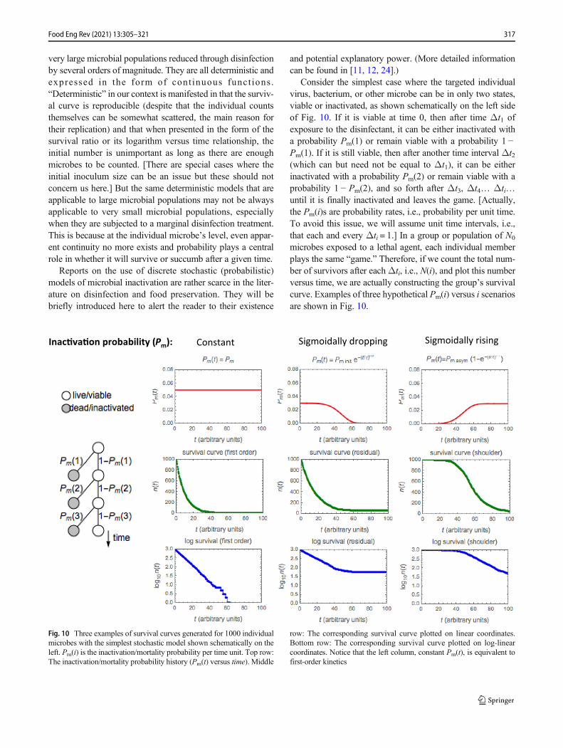
Consider the simplest case where the targeted individualvirus, bacterium, or other microbe can be in only two states,viable or inactivated, as shown schematically on the left sideof Fig. 10. If it is viable at time 0, then after time Δt1 ofexposure to the disinfectant, it can be either inactivated witha probability Pm(1) or remain viable with a probability 1 −Pm(1). If it is still viable, then after another time interval Δt2(which can but need not be equal to Δt1), it can be eitherinactivated with a probability Pm(2) or remain viable with aprobability 1 − Pm(2), and so forth after Δt3, Δt4… Δti…until it is finally inactivated and leaves the game. [Actually,the Pm(i)s are probability rates, i.e., probability per unit time.To avoid this issue, we will assume unit time intervals, i.e.,that each and every Δti = 1.] In a group or population of N0

microbes exposed to a lethal agent, each individual memberplays the same “game.” Therefore, if we count the total num-ber of survivors after eachΔti, i.e., N(i), and plot this numberversus time, we are actually constructing the group’s survivalcurve. Examples of three hypothetical Pm(i) versus i scenariosare shown in Fig. 10.

Constant Sigmoidally dropping Sigmoidally risingInac�va�on probability (Pm):

Fig. 10 Three examples of survival curves generated for 1000 individualmicrobes with the simplest stochastic model shown schematically on theleft. Pm(i) is the inactivation/mortality probability per time unit. Top row:The inactivation/mortality probability history (Pm(t) versus time). Middle

row: The corresponding survival curve plotted on linear coordinates.Bottom row: The corresponding survival curve plotted on log-linearcoordinates. Notice that the left column, constant Pm(t), is equivalent tofirst-order kinetics

317Food Eng Rev (2021) 13:305–321

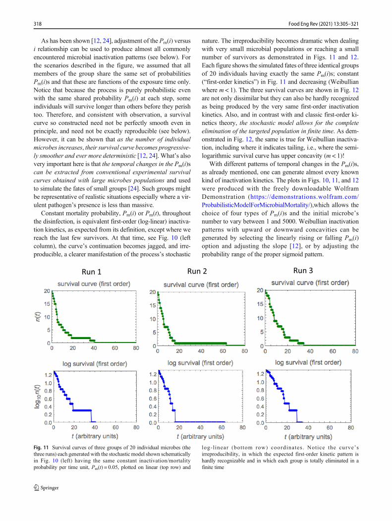
As has been shown [12, 24], adjustment of the Pm(i) versusi relationship can be used to produce almost all commonlyencountered microbial inactivation patterns (see below). Forthe scenarios described in the figure, we assumed that allmembers of the group share the same set of probabilitiesPm(i)s and that these are functions of the exposure time only.Notice that because the process is purely probabilistic evenwith the same shared probability Pm(i) at each step, someindividuals will survive longer than others before they perishtoo. Therefore, and consistent with observation, a survivalcurve so constructed need not be perfectly smooth even inprinciple, and need not be exactly reproducible (see below).However, it can be shown that as the number of individualmicrobes increases, their survival curve becomes progressive-ly smoother and ever more deterministic [12, 24]. What’s alsovery important here is that the temporal changes in the Pm(i)scan be extracted from conventional experimental survivalcurves obtained with large microbes populations and usedto simulate the fates of small groups [24]. Such groups mightbe representative of realistic situations especially where a vir-ulent pathogen’s presence is less than massive.

Constant mortality probability, Pm(i) or Pm(t), throughoutthe disinfection, is equivalent first-order (log-linear) inactiva-tion kinetics, as expected from its definition, except where wereach the last few survivors. At that time, see Fig. 10 (leftcolumn), the curve’s continuation becomes jagged, and irre-producible, a clearer manifestation of the process’s stochastic

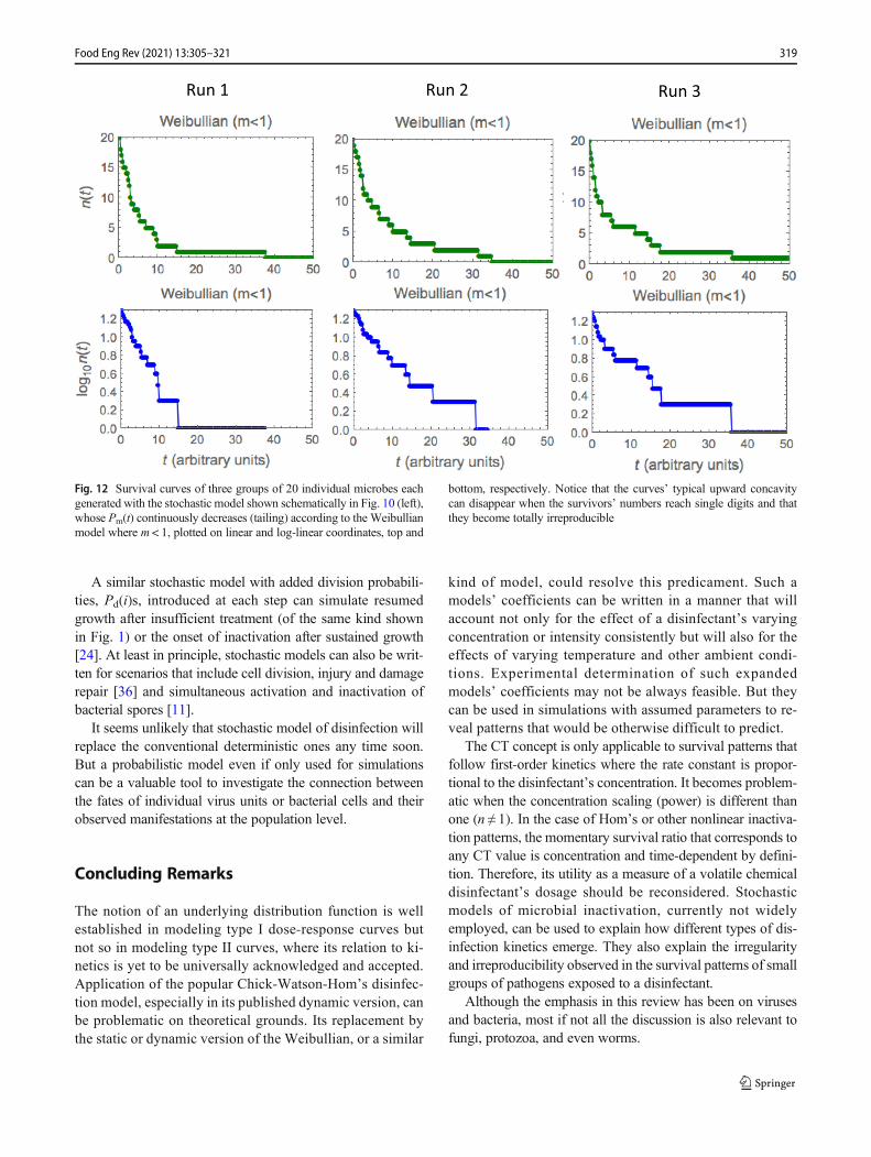
nature. The irreproducibility becomes dramatic when dealingwith very small microbial populations or reaching a smallnumber of survivors as demonstrated in Figs. 11 and 12.Each figure shows the simulated fates of three identical groupsof 20 individuals having exactly the same Pm(i)s; constant(“first-order kinetics”) in Fig. 11 and decreasing (Weibullianwhere m < 1). The three survival curves are shown in Fig. 12are not only dissimilar but they can also be hardly recognizedas being produced by the very same first-order inactivationkinetics. Also, and in contrast with and classic first-order ki-netics theory, the stochastic model allows for the completeelimination of the targeted population in finite time. As dem-onstrated in Fig. 12, the same is true for Weibullian inactiva-tion, including where it indicates tailing, i.e., where the semi-logarithmic survival curve has upper concavity (m < 1)!

With different patterns of temporal changes in the Pm(i)s,as already mentioned, one can generate almost every knownkind of inactivation kinetics. The plots in Figs. 10, 11, and 12were produced with the freely downloadable WolframDemonstration (https://demonstrations.wolfram.com/ProbabilisticModelForMicrobialMortality/),which allows thechoice of four types of Pm(i)s and the initial microbe’snumber to vary between 1 and 5000. Weibullian inactivationpatterns with upward or downward concavities can begenerated by selecting the linearly rising or falling Pm(i)option and adjusting the slope [12], or by adjusting theprobability range of the proper sigmoid pattern.

Run 1 Run 2 Run 3

Fig. 11 Survival curves of three groups of 20 individual microbes (thethree runs) each generated with the stochastic model shown schematicallyin Fig. 10 (left) having the same constant inactivation/mortalityprobability per time unit, Pm(t) = 0.05, plotted on linear (top row) and

log- l inear (bot tom row) coordinates . Not ice the curve’sirreproducibility, in which the expected first-order kinetic pattern ishardly recognizable and in which each group is totally eliminated in afinite time

318 Food Eng Rev (2021) 13:305–321

A similar stochastic model with added division probabili-ties, Pd(i)s, introduced at each step can simulate resumedgrowth after insufficient treatment (of the same kind shownin Fig. 1) or the onset of inactivation after sustained growth[24]. At least in principle, stochastic models can also be writ-ten for scenarios that include cell division, injury and damagerepair [36] and simultaneous activation and inactivation ofbacterial spores [11].

It seems unlikely that stochastic model of disinfection willreplace the conventional deterministic ones any time soon.But a probabilistic model even if only used for simulationscan be a valuable tool to investigate the connection betweenthe fates of individual virus units or bacterial cells and theirobserved manifestations at the population level.

Concluding Remarks

The notion of an underlying distribution function is wellestablished in modeling type I dose-response curves butnot so in modeling type II curves, where its relation to ki-netics is yet to be universally acknowledged and accepted.Application of the popular Chick-Watson-Hom’s disinfec-tion model, especially in its published dynamic version, canbe problematic on theoretical grounds. Its replacement bythe static or dynamic version of the Weibullian, or a similar

kind of model, could resolve this predicament. Such amodels’ coefficients can be written in a manner that willaccount not only for the effect of a disinfectant’s varyingconcentration or intensity consistently but will also for theeffects of varying temperature and other ambient condi-tions. Experimental determination of such expandedmodels’ coefficients may not be always feasible. But theycan be used in simulations with assumed parameters to re-veal patterns that would be otherwise difficult to predict.

The CT concept is only applicable to survival patterns thatfollow first-order kinetics where the rate constant is propor-tional to the disinfectant’s concentration. It becomes problem-atic when the concentration scaling (power) is different thanone (n ≠ 1). In the case of Hom’s or other nonlinear inactiva-tion patterns, the momentary survival ratio that corresponds toany CT value is concentration and time-dependent by defini-tion. Therefore, its utility as a measure of a volatile chemicaldisinfectant’s dosage should be reconsidered. Stochasticmodels of microbial inactivation, currently not widelyemployed, can be used to explain how different types of dis-infection kinetics emerge. They also explain the irregularityand irreproducibility observed in the survival patterns of smallgroups of pathogens exposed to a disinfectant.

Although the emphasis in this review has been on virusesand bacteria, most if not all the discussion is also relevant tofungi, protozoa, and even worms.

Run 1 Run 2 Run 3

Fig. 12 Survival curves of three groups of 20 individual microbes eachgenerated with the stochastic model shown schematically in Fig. 10 (left),whose Pm(t) continuously decreases (tailing) according to the Weibullianmodel where m < 1, plotted on linear and log-linear coordinates, top and

bottom, respectively. Notice that the curves’ typical upward concavitycan disappear when the survivors’ numbers reach single digits and thatthey become totally irreproducible

319Food Eng Rev (2021) 13:305–321

Acknowledgments The author thanks Mr. Mark D. Normand, for pro-gramming the Wolfram Demonstrations and other software on whichmuch of the discussion is based, and to Dr. Matthew D. Moore for pro-viding an important relevant piece of information.

References

1. Anon (2017) Enteric viruses in drinking water. Document forPublic Consultation Health Canada (On the Internet)

2. Aragao GMF, Corradini MG, Normand MD, Peleg M (2007)Evaluation of the Weibull and log-normal distribution functionsas survival models of Escherichia coli under isothermal and non-isothermal conditions. Int J Food Microbiol 19:243–257

3. Bosch A, Pinto RM, Guix S (2016) Foodborne viruses. CurrntOpinion Food Sci 8:110–119

4. Bozkurt H, D’Souza DH, Davidson PM (2015) Thermal inactiva-tion kinetics of human norovirus surrogates and hepatitis A virus inTurkey deli meat. Appl Environ Microbiol 81:4850–5859

5. Brennecke M (2009) Disinfection kinetics of virus aggregates ofbacteriophage MS2. Master Thesis. Laboratory of EnvironmentalChemistry, Ecole Polytechnique Federale de Lausanne. Lausanne,Switzerland

6. Brown WK, Wohletz KH (1995) Derivation of the Weibull distri-bution based on physical connection to the Rosin-Rammler andlognormal distributions. J Appl Phys 78:2758–2763

7. Chick H (1908) Investigation of the laws of disinfection. EpidemiolInfect

8. Buzrul S (2017) Evaluation of different dose-response models forhigh hydrostatic pressure inactivation of microorganisms. Foods6(79):1–17

9. Chick H (1908) Investigation of the laws of disinfection. EpidemiolInfect 8:92–158

10. CookN, Knight A, Richards GP (2016) Persistence and eliminationof human norovirus in food and on food contact surfaces: a criticalreview. J Food Protect 79:1273–1294

11. Corradini MG, Normand MD, Eisenberg M, Peleg M (2010)Evaluation of a stochastic inactivation model for heat-activatedspores of Bacillus spp. Appl Environ Microbiol 76:4402–4412

12. Corradini MG, Normand MD, Peleg M (2010) A stochastic anddeterministic model of microbial heat inactivation. J Food Sci 75:R59–R70

13. Corradini MG, Peleg M (2003) A model of microbial survivalcurves in water treated with a volatile disinfectant. J ApplMicrobiol 95:1268–1276

14. Ganguly P, Byrnea C, Breen A, Pillai SC (2018) Antimicrobialactivity of photocatalysts: fundamentals, mechanisms, kineticsand recent advances. Appl Catalysis B: Environmental 225:51–75

15. Garba CP (2015) Disinfection. Chapter 29. In: Pepper IA, GerbaCP, Gentry TJ (eds) Environmental microbiology, 3rd edn.Elsevier, pp 645–662

16. Gil MM, Miller FA, Brandao TRS, Silva CLM (2017)Mathematical models for prediction of temperature effects on ki-netic parameters of microorganisms’ inactivation: tools for modelcomparison and adequacy in data fitting. Food Bioproc Technol10:2208–2225

17. Guzel-Seydim ZB, Greene AK, SeydimAC (2004) Use of ozone inthe food industry. LWT 37:453–460

18. Gyurek LL, Finch GR (1998) Modeling water treatment chemicaldisinfection kinetics. J Environ Eng 9:783–793

19. Haas CN, Joffe J, Anmangandla U, Tacangelo JG, Heath M (1996)Water quality and disinfection kinetics. J AWWA 88:95–103

20. Haas CN, Joffe J (1994) Disinfection under dynamic conditions:modification of Hom’s model for decay. Environ Sci Technol 28:1367–1469

21. Haas CN, Kara SB (1984) Kinetics of microbial inactivation bychlorine - I Review of results in demand free systems. Water Res11:1443–1449

22. Haas CN, Rose JB, Gerba C, Regli S (1993) Risk assessment ofvirus in drinking water. Risk Assess 13:545–552

23. Hijnen WAM, Beerendonk EF, Medema GJ (2006) Inactivationcredit of UV radiation for viruses, bacteria and protozoan(oo)cysts in water: a review. Water Res 40:3–22

24. Horowitz J, Normand MD, Corradini MG, Peleg M (2010) A prob-abilistic model of growth, division and mortality of microbial cells.Appl Environ Microbiol 76:230–242

25. Jones RM, Su Y-M (2015) Dose-response models for selected re-spiratory infectious agents: Bordetella pertussis, group aStreptococcus, rhinovirus and respiratory syncytial virus. BMCInfect Diseases 15:90 (1-9)

26. Joshi K, Mahendran R, Alagusundaram K, Norton T, Tiwari BK(2013) Novel disinfectants for fresh produce. Trends Food SciTechnol 34:54–61

27. KitajimaM, Huamg Y,Watanabe T, Katayama H, Haas CN (2011)Dose–response time modelling for highly pathogenic avian influ-enza A (H5N1) virus infection. Letter Appl Microbiol 53:438–444

28. Lambert RJW, Johnston MD (2000) Disinfection kinetics: a newhypothesis and model for the tailing of log-survivor/time curves. JAppl Micobiol 88:907–913

29. Mattle MJ, Crouzy B, Brennecke M, Wigginton KR, Perona P,Kohn T (2011) Impact of virus aggregation on inactivation byperacetic acid an implications for other disinfectants. Environ SciTechnol 45:7710–7717

30. Messner MJ, Berger P, Nappier SP (2014) Fractional Poisson – asimple dose response model for human norovirus. Risk Anal 34:1820–1829

31. Misra NN, Tiwari BK, Raghavarao KSMS (2011) Nonthermalplasma inactivation of food-borne pathogens. Food Eng Rev 3:159–170

32. Najm I (2006) An alternative interpretation of disinfection kinetics.J AWWA 98:93–101

33. Peleg M (1996) Evaluation of the Fermi equation as a model ofdose-response curves. Appl Microbiol Biotechnol 46:303–306

34. Peleg M (2000) Microbial survival curves – the reality of flat“shoulders” and thermal death times. Food Res Int 33:531–538

35. Peleg M (2006) Advanced quantitative microbiology for food andbiosystems: models for predicting growth and inactivation. CRCPress, Boca Raton FL

36. Peleg M (2017) Modeling microbial inactivation by pulsed electricfields. In: Miklavcic D (ed) Handbook of electroporation. Springer,pp 1269–1286

37. Peleg M, Normand MD (2004) Calculating microbial survival pa-rameters and predicting survival curves from non-isothermal inac-tivation data. Crit Rev Food Sci Nut 44:409–418

38. PelegM,NormandMD, CorradiniMG (2011) Construction of foodandwater borne pathogens’ dose-response curves using the expand-ed Fermi solution. J Food Sci 76:R82–R89

39. PelegM, NormandMD, CorradiniMG (2012) The Arrhenius equa-tion revisited. Crit Rev Food Sci Nut 52:830–851

40. Peleg M, Normand MD, Damrau E (1997) Mathematical interpre-tation of dose-response curves. Bull Math Biol 59:747–761

41. Peleg M, Normand MD, Horowitz J, Corradini MG (2007) Anexpanded Fermi solution for microbial risk assessment. Intrn JFood Microbiol 113:92–101

42. Peleg M, Normand MD, Horowitz J, Corradini MG (2011)Expanded Fermi solution for estimating the survival of ingestedpathogenic and probiotic microbial cells and spores. ApplEnviron Microbiol 77:312–319

43. Pressman JG, Wahman DG (2019) Understanding disinfection re-siduals. EPA Office of R&D EPA.GOV

320 Food Eng Rev (2021) 13:305–321

44. Rossi S, Antonelli M, Mezzanotte V, Nurizzo C (2007) Peraceticacid disinfection: a feasible alternative to wastewater chlorination.Water Environ Res 79:341–350

45. Shereen MA, Khan S, Kazmi A, Bashir N, Siddique R (2020)COVID-19 infection: origin, transmission, and characteristics ofhuman coronaviruses. J Adv Res 24:91–98

46. Sigstam T, Rohatschek A, Zhong Q, Brennecke M, Kohn T (2014)On the cause of the tailing phenomenon during virus disinfection bychlorine dioxide. Water Res 48:82–89

47. Sigstam T, Gannon G, Cascella M, Pecson BM, Wigginton KR,Kohn T (2013) Subtle differences in virus composition affect dis-infection kinetics and mechanisms. Appl Envirn Microbiol 79:3455–3467

48. Teunis PEM, Havelaar AH (2000) The beta Poisson dose-responsemodel is not a single-hit model. Risk Anal 20:513–520

49. Thurston-Enriquez JA, Haas CN, Jacangelo J, Greba CP (2005)Inactivation of enteric adenovirus and feline calicivirus by chlorinedioxide. Appl Environ Microbiol 71:3100–3105

50. Van Boekel MAJS (2002) On the use of the Weibull model todescribe thermal inactivation of microbial vegetative cells. Intnl JFood Microbiol 74:139–159

51. Van Boekel MAJS (2008) Kinetic modeling of food quality: areview. Comp Rev Food Sci Food Safety 7:144–158

52. Verhaelen K, Bouwknegt M, Lodder-Verschoor F, Rutjes SA, deRoda Husman AM (2012) Persistence of human norovirus GII.4and GI.4, murine norovirus, and human adenovirus on soft berriesas compared with PBS at commonly applied storage conditions.Intnl J Food Microbiol 160:137–144

53. Watanabe T, Bartrand TA, Omura T, Haas CN (2012) Dose-response assessment for influenza A virus based on data sets ofinfection with its live attenuated reassortants. Risk Anal 32:555–565

54. Watson HE (1908) A note on the variation of the rate of disinfectionwith change in the concentration of the disinfectant. EpidemiolInfect 8:536–542

55. Weir MH, Mitchell J, Flynn W, Pope JM (2017) Development of amicrobial dose response visualization andmodelling application forQMRA modelers and educators. Environ Modelling Software 88:74–83

56. Xie G, Roiko A, Stratton H, Lemckert C, Dunn PK, Mengersen K(2017) Guidelines for use of the approximate beta-Poisson dose–response model. Risk Anal 37:1388–1402

Publisher’s Note Springer Nature remains neutral with regard to jurisdic-tional claims in published maps and institutional affiliations.

321Food Eng Rev (2021) 13:305–321