Microarray data analysis –Gold-mining in a minefield

Matthias E. Futschik

Institute for Theoretical Biology

Medical Devision (Charité),

Humboldt-University, Berlin, Germany

MIR@W, Warwick Mathematics Institut, 15 November 2004

Outline● The Gold-mine

● Stake out the claim ● Microarray Boom: 10 years● What can we learn from Greek philosophy?

● Minefield I : Microarray is not equal microarray● Microarray technologies: Do we measure the same?

● Minefield II: Microarrays (almost) always find something ● Read-out, design and validation

●Minefield III: Not everything is gold that shines● Error detection and correction

●Minefield IV: Choosing the right sieve.● Significance of differential gene expression

●Minefield V: There is more than just nuggets and soil● Soft clustering delivers gray values

●Conclusions

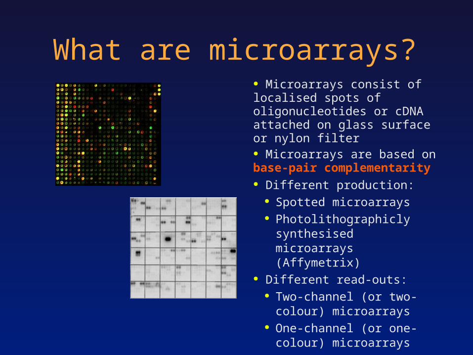
What are microarrays?● Microarrays consist of localised spots of oligonucleotides or cDNA attached on glass surface or nylon filter● Microarrays are based on base-pair complementarity● Different production:

● Spotted microarrays● Photolithographicly synthesised

microarrays (Affymetrix)● Different read-outs:

● Two-channel (or two-colour) microarrays

● One-channel (or one-colour) microarrays

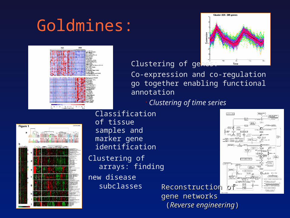
Goldmines:

Clustering of arrays: finding

new disease subclasses

Clustering of genes:

Co-expression and co-regulation go together enabling functional annotation

Clustering of time series

Reconstruction of Reconstruction of gene networksgene networks ((Reverse engineeringReverse engineering))

Classification of tissue samples and marker gene identification

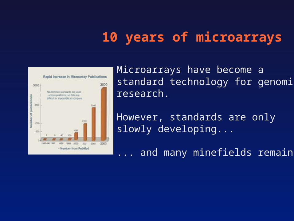
10 years of microarrays

Microarrays have become astandard technology for genomicsresearch.

However, standards are only slowly developing...

... and many minefields remain.

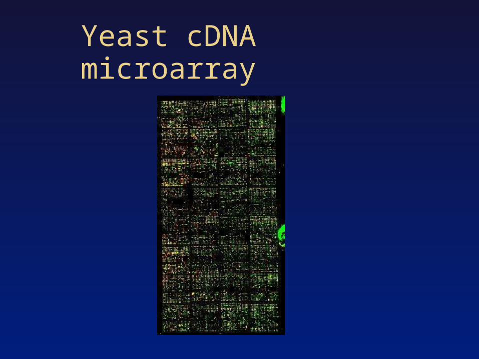
Yeast cDNA microarray

Plato’s CaveAND now, I said, let me show in a figure

how far our nature is enlightened or unenlightened:

Behold! Human beings living in a underground den,

which has a mouth open towards the light and

reaching all along the den; here they have been from their childhood, and have their leg and

necks chained so that they cannot move, and can only see before them, being prevented by the

chains from turning round their heads. Above and behind them a fire is blazing at a distance, and between the fire and the

prisoners there is a raised way; and you will see, if you look, a low wall built along the way, like the screen which

marionette players have in front of them, over which they show the puppets….

To them, I said, the truth would be literally nothing but the shadows of the images…

And now look again, and see what will naturally follow if the prisoners are released and disabused of their error.

At first, when any of them is liberated and compelled suddenly to stand up and

turn his neck round and walk and look towards the light, he will suffer sharp pains; the glare will

distress him, and he will be unable to see the realities of which in his former state he had seen the

shadows; and then conceive some one saying to him, that what he saw before was an illusion, but

that now, when he is approaching nearer to being and his eye is turned towards more real

existence, he has a clearer vision,…

The Challange

MicroarraysMicroarraysThousands of simultaneously measured gene activitiesThousands of simultaneously measured gene activities

Genetic networksGenetic networksComplex regulation of gene expressionComplex regulation of gene expression

Medical Medical applicationsapplicationsNew drug discovery New drug discovery based on detailed based on detailed molecular models molecular models

Minefield I :Microarray is not equal micorarray

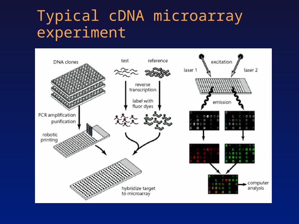
Typical cDNA microarray experiment

Microarray technology I Two-colour microarray (cDNA and spotted oligonucleotide

microarrays) Probes are PCR products based on a chosen cDNA library or synthesized

oligonucleotides (length 50-70) optimized for specifity and binding properties >> probe design

Probes are mechanically spotted. To control variation of amount of printed cDNA/oligos and spot morphology, reference RNA sample is included. Thus, ratios are considered as basic units for analysing gene expression. Absolute intensities should be interpreted with care.

MOVIE 1: Array production - Galbraith labMOVIE 1: Array production - Galbraith lab

MOVIE 2: Principles – Schreiber lab MOVIE 2: Principles – Schreiber lab

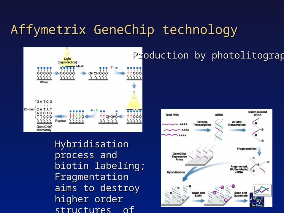
Affymetrix GeneChip technologyAffymetrix GeneChip technology

Production by photolitographyProduction by photolitography

Hybridisation process Hybridisation process and biotin labelíng;and biotin labelíng;Fragmentation aims to Fragmentation aims to destroy higher order destroy higher order structures of cRNAstructures of cRNA

Microarray technologies II One-colour microarrays (Affymetrix GeneChips)

Measurement of hybridisation of target RNA to sets of 25-oligonucleotides (probes).

Probes are paired: Perfect match (PM) and mis-match (MM). PM are complementary to the gene sequence of interest. MM include a single nucleotide changed in the middle position of the oligonucleotide. MM serve for controlling of experimental variation and non-specific cross-hybridisation. Thus, MMs constitute internal references (on the probe site).

Average (PM-MM) delivers measure for gene expression. However, different methods to calculates summary indices exist (e.g. MAS,dchip, RMA...)

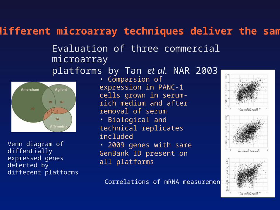
Do different microarray techniques deliver the same?

Evaluation of three commercial microarrayplatforms by Tan et al. NAR 2003

Venn diagram of diffentially expressed genes detected by different platforms

Correlations of mRNA measurements

• Comparsion of expression in PANC-1 cells grown in serum-rich medium and after removal of serum • Biological and technical replicates included • 2009 genes with same GenBank ID present on all platforms

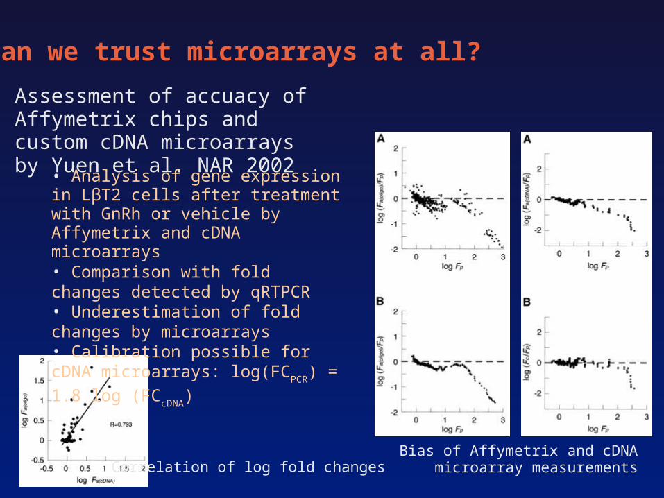
Can we trust microarrays at all?

Assessment of accuacy of Affymetrix chips and custom cDNA microarrays by Yuen et al. NAR 2002

Correlation of log fold changesBias of Affymetrix and cDNA microarray

measurements

• Analysis of gene expression in LβT2 cells after treatment with GnRh or vehicle by Affymetrix and cDNA microarrays• Comparison with fold changes detected by qRTPCR • Underestimation of fold changes by microarrays• Calibration possible for cDNA microarrays: log(FC

PCR) = 1.8 log (FC

cDNA)

Minefield II :Microarray always find something

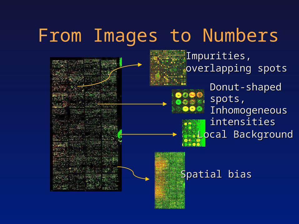
From Images to NumbersImpurities, Impurities, overlapping spotsoverlapping spots

Donut-shaped spots, Donut-shaped spots, Inhomogeneous Inhomogeneous intensitiesintensities

Local BackgroundLocal Background

Spatial biasSpatial bias

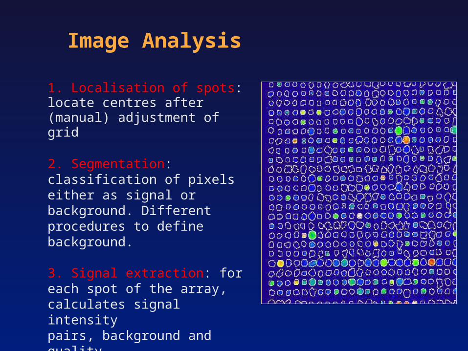
Image Analysis

1. Localisation of spots: locate centres after (manual) adjustment of grid

2. Segmentation: classification of pixels either as signal or background. Different procedures to define background.

3. Signal extraction: for each spot of the array, calculates signal intensity pairs, background and quality measures.

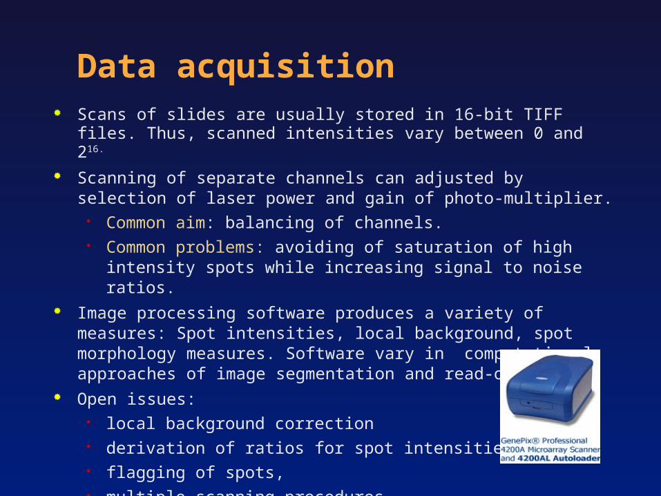
Data acquisition Scans of slides are usually stored in 16-bit TIFF files. Thus, scanned intensities

vary between 0 and 216. Scanning of separate channels can adjusted by selection of laser power and gain

of photo-multiplier. Common aim: balancing of channels. Common problems: avoiding of saturation of high intensity spots while

increasing signal to noise ratios. Image processing software produces a variety of measures: Spot intensities,

local background, spot morphology measures. Software vary in computational approaches of image segmentation and read-out.

Open issues: local background correction derivation of ratios for spot intensities flagging of spots, multiple scanning procedures

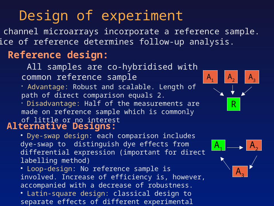
Design of experimentTwo channel microarrays incorporate a reference sample. Choice of reference determines follow-up analysis.

A1

A2 A

3

R

Reference design: All samples are co-hybridised with common reference sample● Advantage: Robust and scalable. Length of path of direct comparison equals 2.● Disadvantage: Half of the measurements are made on reference sample which is commonly of little or no interest

Alternative Designs:● Dye-swap design: each comparison includes dye-swap to distinguish dye effects from differential expression (important for direct labelling method) ● Loop-design: No reference sample is involved. Increase of efficiency is, however, accompanied with a decrease of robustness.● Latin-square design: classical design to separate effects of different experimental factors

A1

A2

A3

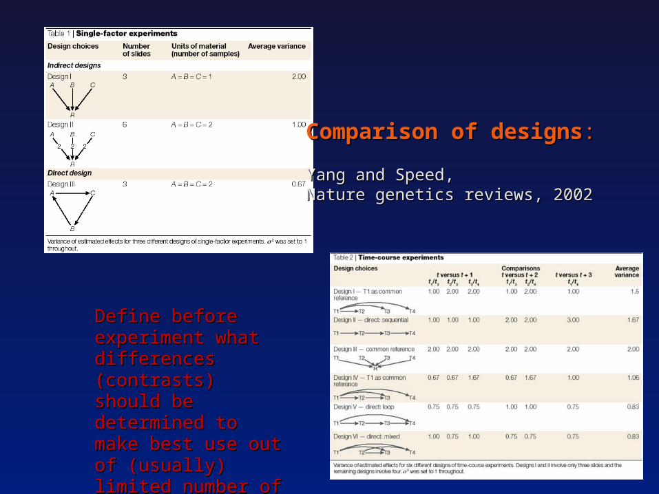
Comparison of designsComparison of designs::

Yang and Speed, Yang and Speed, Nature genetics reviews, 2002Nature genetics reviews, 2002

Define before experiment Define before experiment what differences (contrasts) what differences (contrasts) should be determined to should be determined to make best use out of make best use out of (usually) limited number of (usually) limited number of arraysarrays

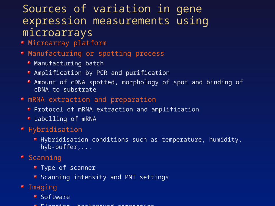
Sources of variation in gene expression measurements using microarrays

Microarray platform

Manufacturing or spotting process

Manufacturing batch

Amplification by PCR and purification

Amount of cDNA spotted, morphology of spot and binding of cDNA to substrate

mRNA extraction and preparation

Protocol of mRNA extraction and amplification

Labelling of mRNA

Hybridisation

Hybridisation conditions such as temperature, humidity, hyb-buffer,...

Scanning

Type of scanner

Scanning intensity and PMT settings

Imaging

Software

Flagging, background correction,...

Planning an microarray experiment Essentials:

●Technical replicates assess variability induced by experimental procedures.

● Biological replicates (assess generality of results).

● Number of replicates depends on desired sensitivity and sensibility of measurements and research goal.

● Randomisation to avoid confounding of experimental factors. Blocking to reduce number of experimental factors.

● Control spots assess reproducibility within and between array, background intensity, cross-hybridisation and/or sensitivity of measurement. They can consists of empty spots or hybridisation-buffer, genomic DNA, foreign DNA, house-holding genes of foreign (non-cross-hybridising) cDNA.

● Validation of results is crucial ● by other experimental techniques (e.g. Northern, RT-PCR) ● By comparison with independent experiments.

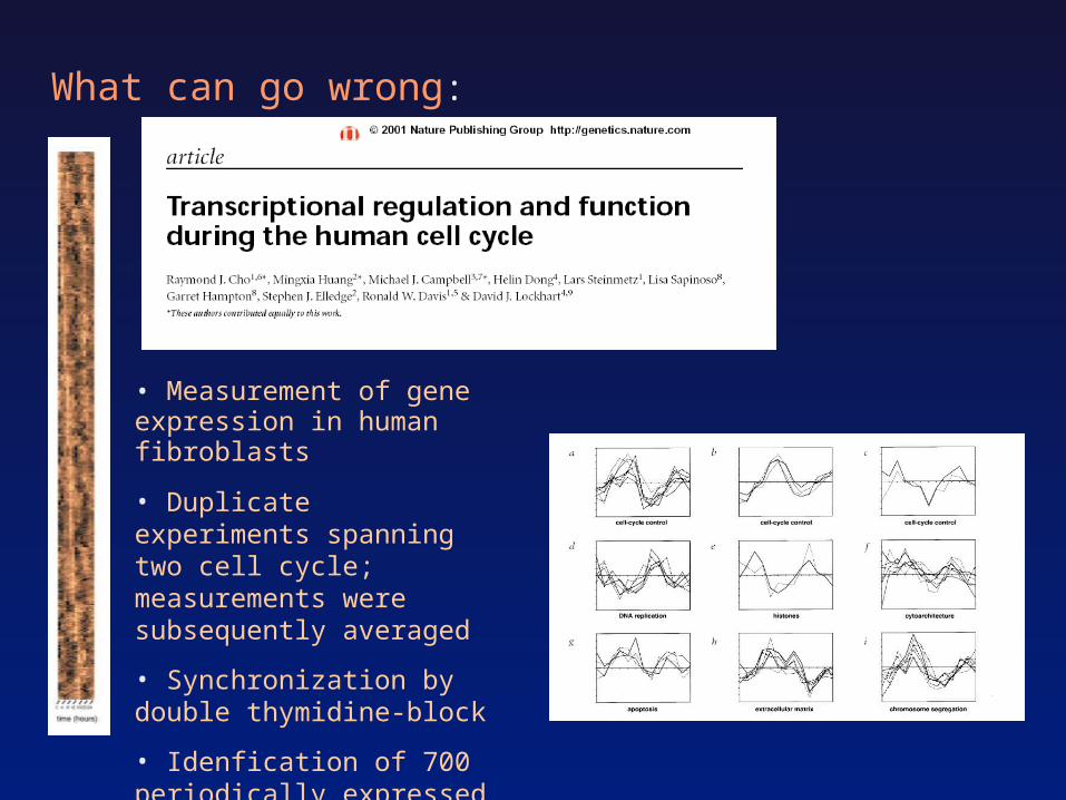
What can go wrong:

• Measurement of gene expression in human fibroblasts

• Duplicate experiments spanning two cell cycle; measurements were subsequently averaged

• Synchronization by double thymidine-block

• Idenfication of 700 periodically expressed genes (300 uncharacterized ESTs)

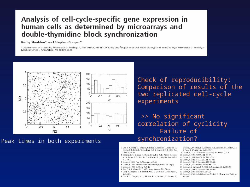
Check of reproducibility: Comparison of results of the two replicated cell-cycle experiments

>> No significant correlation of cyclicity Failure of synchronization?

Peak times in both experiments

Minefield III :Not everything is gold that shines

Data-Preprocessing

Background subtraction: May reduce spatial artefacts May increase variance as both

foreground and background intensities are estimates ( “arrow-like” plots MA-plots)

Preprocessing: Thresholding: exclusion of low

intensity spots or spots that show saturation

Transformation: A common transformation is log-transformation for stabilitation of variance across intensity scale and detection of dye related bias.

Log-transformationLog-transformation

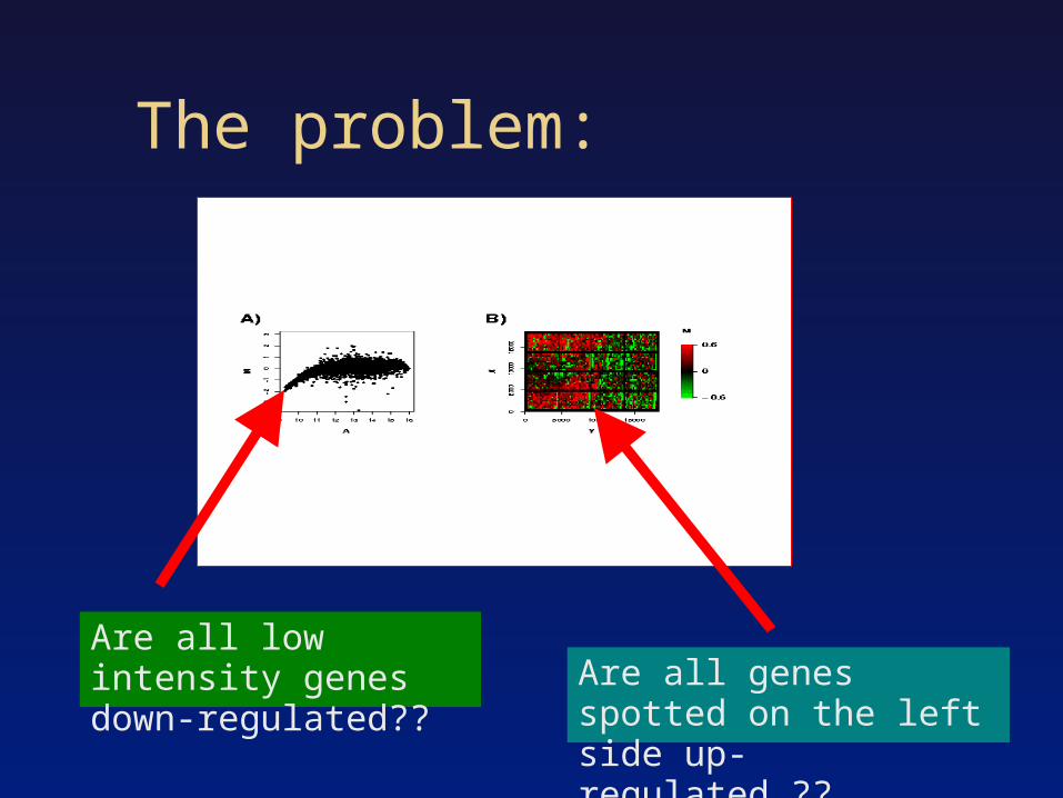
The problem:

Are all low intensity genes down-regulated?? Are all genes spotted on the

left side up-regulated ??

Normalization – bending data to make it look nicer...

Normalization describes a variety of data transformations aiming to correct for experimental variation

Within – array normalization

Normalization based on 'householding genes' assumed to be equally expressed in different samples of interest

Normalization using 'spiked in' genes: Ajustment of intensities so that control spots show equal intensities across channels and arrays

Global linear normalisation assumes that overall expression in samples is constant. Thus, overall intensitiy of both channels is linearly scaled to have value.

Non-linear normalisation assumes symmetry of differential

expression across intensity scale and spatial dimension of array

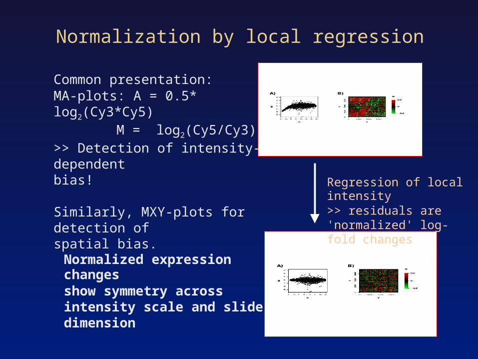
Normalization by local regression

Regression of local intensity >> residuals are 'normalized' log-fold changes

Common presentation:MA-plots: A = 0.5* log2(Cy3*Cy5)

M = log2(Cy5/Cy3)>> Detection of intensity-dependentbias!

Similarly, MXY-plots for detection of spatial bias.

Normalized expression changesshow symmetry across intensity scale and slide dimension

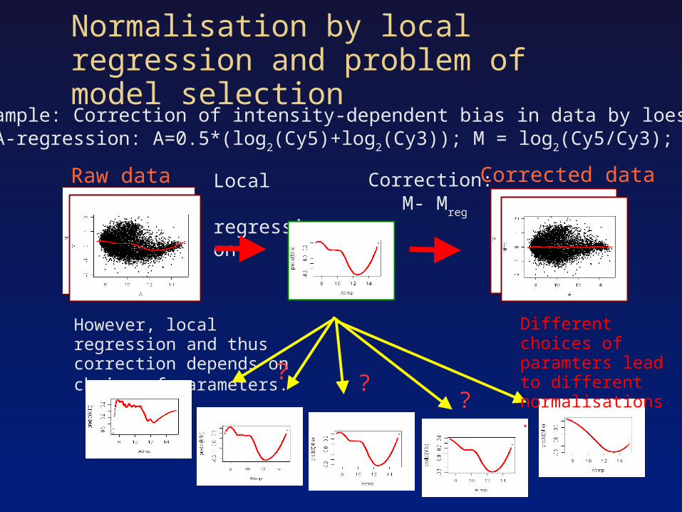
Normalisation by local regression and problem of model selection

Example: Correction of intensity-dependent bias in data by loess (MA-regression: A=0.5*(log

2(Cy5)+log

2(Cy3)); M = log

2(Cy5/Cy3);

Raw data Local regression

Corrected data

However, local regression and thus correction depends onchoice of parameters.

Correction: M- M

reg

? ??

Different choices of paramters lead to different normalisations.

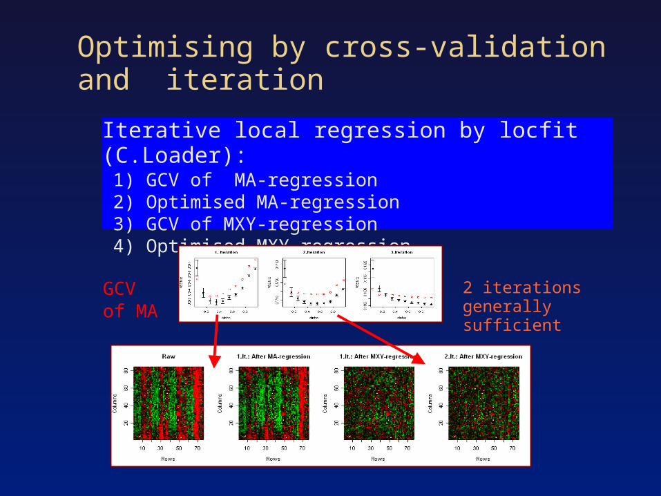
Optimising by cross-validation and iteration

Iterative local regression by locfit (C.Loader): 1) GCV of MA-regression 2) Optimised MA-regression 3) GCV of MXY-regression 4) Optimised MXY-regression

2 iterations generally sufficient

GCV of MA

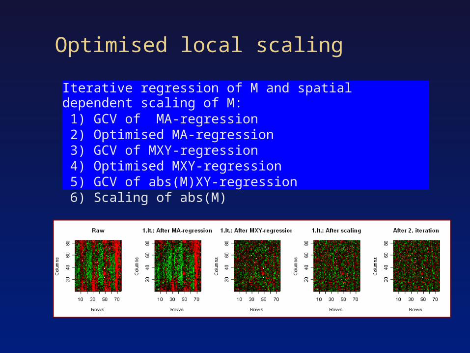
Optimised local scaling

Iterative regression of M and spatial dependent scaling of M: 1) GCV of MA-regression 2) Optimised MA-regression 3) GCV of MXY-regression 4) Optimised MXY-regression 5) GCV of abs(M)XY-regression 6) Scaling of abs(M)

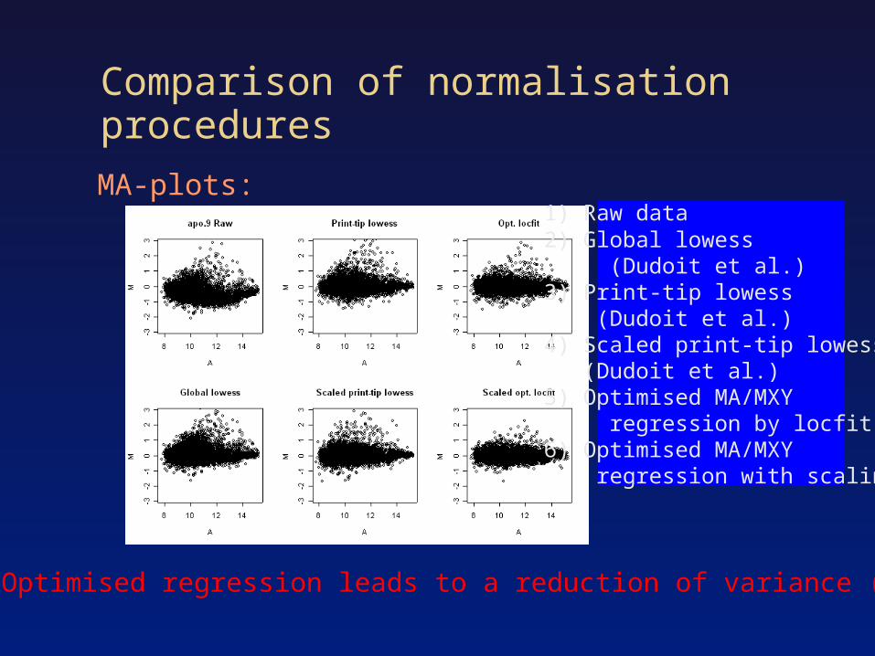
Comparison of normalisation procedures

MA-plots: 1) Raw data 2) Global lowess (Dudoit et al.) 3) Print-tip lowess (Dudoit et al.) 4) Scaled print-tip lowess (Dudoit et al.) 5) Optimised MA/MXY regression by locfit 6) Optimised MA/MXY regression with scaling

=> Optimised regression leads to a reduction of variance (bias)

Comparison II: Spatial distribution

=> Not optimally normalised data show spatial bias

MXY-plots canindicate spatial bias

MXY-plots:

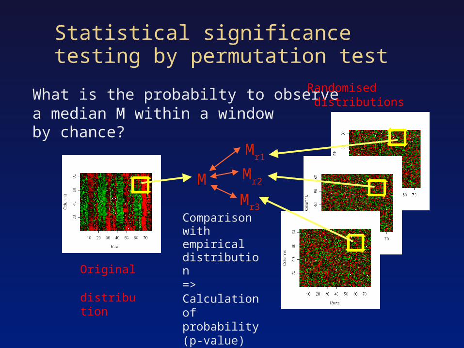
Statistical significance testing by permutation test

M

Original distribution

What is the probabilty to observe a median M within a window by chance?

Comparison with empirical distribution=> Calculation of probability(p-value) using Fisher’s method

Mr1

Mr2

Mr3

Randomised distributions

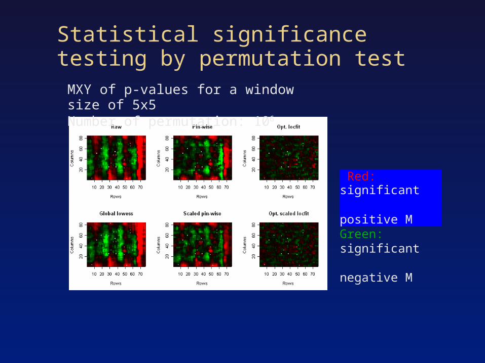
Statistical significance testing by permutation test

MXY of p-values for a window size of 5x5Number of permutation: 106

Red: significant positive MGreen: significant negative M

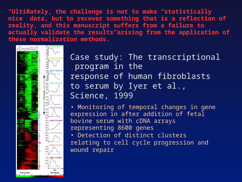
“Ultimately, the challenge is not to make “statistically nice” data, but to recover something that is a reflection of reality, and this manuscript suffers from a failure to actually validate the results arising from the application of these normalization methods.”

Case study: The transcriptional program in the response of human fibroblasts to serum by Iyer et al., Science, 1999

• Monitoring of temporal changes in gene expression in after addition of fetal bovine serum with cDNA arrays representing 8600 genes • Detection of distinct clusters relating to cell cycle progression and wound repair

Verification of microarray measurements by RTPCR

• Correlation of logged fold changes (note underestimation by microarray)• Derivation for COX2 because of “localized area of low intensity on array scan”

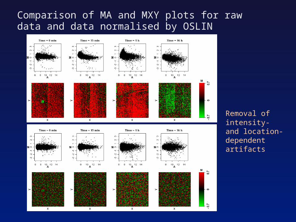
Comparison of MA and MXY plots for raw data and data normalised by OSLIN

Removal of intensity- and location-dependent artifacts

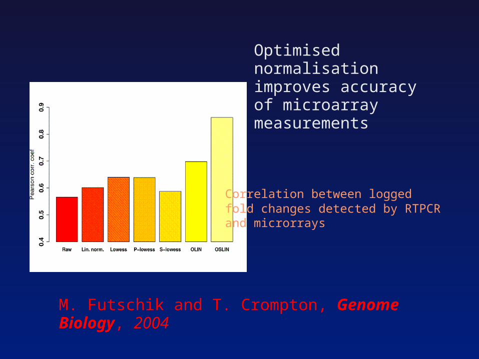
M. Futschik and T. Crompton, Genome Biology, 2004

Optimised normalisation improves accuracy of microarray measurements

Correlation between logged fold changes detected by RTPCRand microrrays

Minefield IV :Choosing the right sieve

Detection of differential expression What makes differential

expression differential expression? What is noise?

Foldchanges are commonly used to quantify differenitial expression but can be misleading (intensity-dependent).

Basic challange: Large number of (dependent/correlated) variables compared to small number of replicates (if any).

Can you spot the interesting spots?

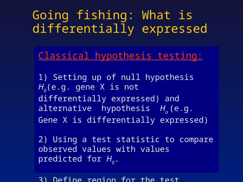
Classical hypothesis testing:

1) Setting up of null hypothesis H0(e.g. gene X is not

differentially expressed) and alternative hypothesis H

a (e.g. Gene X is differentially expressed)

2) Using a test statistic to compare observed values with values predicted for H

0.

3) Define region for the test statistic for which H0 is

rejected in favour of Ha.

Going fishing: What is differentially expressed

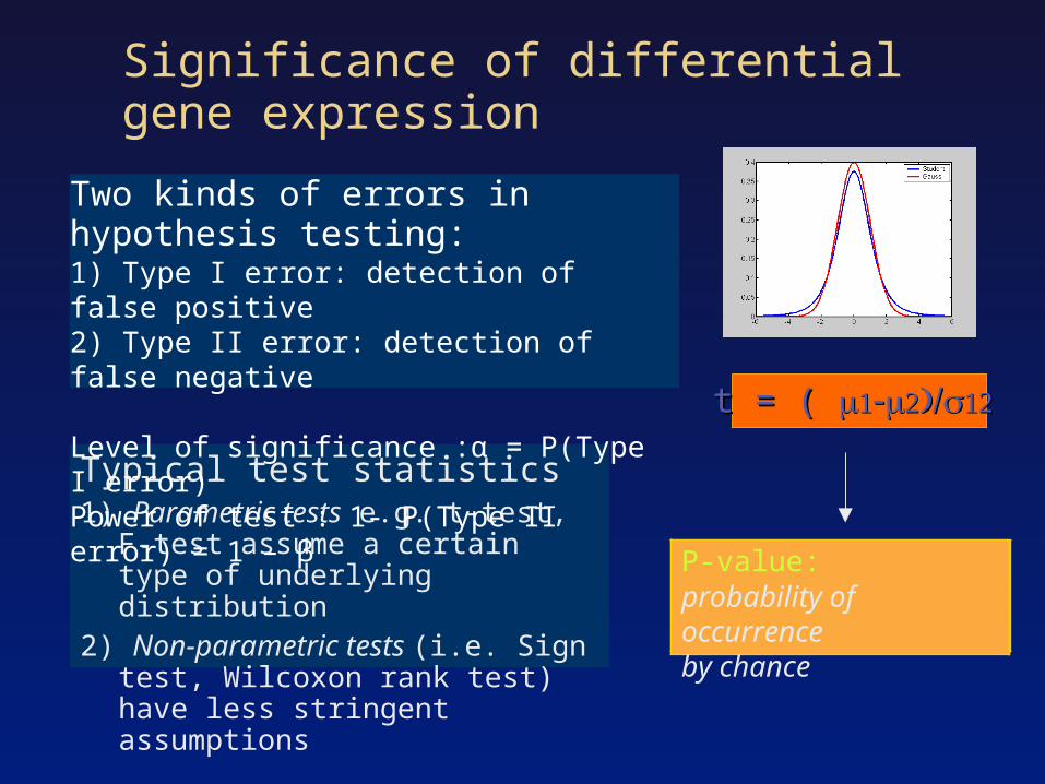
Significance of differential gene expression

Typical test statistics1) Parametric tests e.g. t-test, F-test assume

a certain type of underlying distribution 2) Non-parametric tests (i.e. Sign test,

Wilcoxon rank test) have less stringent assumptions

t = ( t = (

P-value: probability of occurrence by chance

Two kinds of errors in hypothesis testing:1) Type I error: detection of false positive2) Type II error: detection of false negative

Level of significance :α = P(Type I error)Power of test : 1- P(Type II error) = 1 – β

Criteria for gene selection

Accuracy: how closely are the results to the true values

Precision: how variable are the results compared to the true value

Sensitivity: how many true posítive are detected Specificity: how many of the selected genes are

true positives.

>> Multiple testing required with large number of tests but small number of replicates.

>> Adjustment of significance of tests necessary

Example: Probability to find a true H

0 rejected for α=0.01 in 100 independent

tests: P = 1- (1-α) 100 ~ 0.63

Multiple testing poses challanges

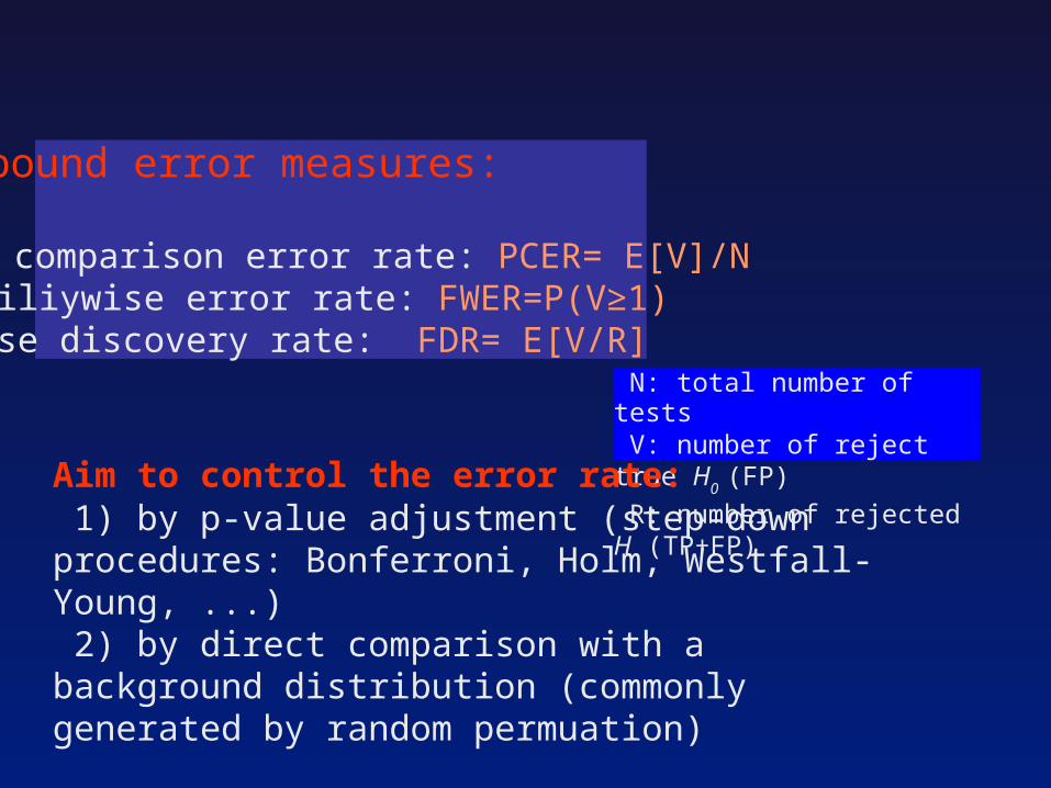
Compound error measures:

Per comparison error rate: PCER= E[V]/N Familiywise error rate: FWER=P(V≥1) False discovery rate: FDR= E[V/R]

N: total number of tests V: number of reject true H

0 (FP)

R: number of rejected H (TP+FP) Aim to control the error rate: 1) by p-value adjustment (step-down procedures: Bonferroni, Holm, Westfall-Young, ...) 2) by direct comparison with a background distribution (commonly generated by random permuation)

Identification of periodically expressed genes in human cell cycle by Whitfield et al., 2002, Molecular Biology of the Cell

• Expression in HeLa cells were monitored using cDNA arrays

• Several synchronization protocols were used to detect artifacts

• 800 genes were detected as periodically expressed by spectral analysis.

A second look reveals doubtful classifications

All genes were identified asperiodically expressed by Whitfield et al.

Wichert et al., Bioinformatics, 2004

Constistency of replications

Case study: SW480/620 cell line comparisonSW480: derived from primary tumourSW 620: derived from lymphnode metastisis of same patient Model for cancer progression

Experimental design:• 4 independent hybridisations (technical replicates)#• 4000 genes

Usage of paired t-test

d

dt

sd: average differences of paired intensitiessd: standard deviation of d

p-value < 0.01 Bonferroni adjusted p-value < 0.01

Robust t-test

2 2 2 tot gene gene exp

Adjust estimation of variance:Compound error model:

Gene-specific error

Experiment-specificerror

This model avoidsselection of control spots

M. Futschik et al, Genome Letters, 2002

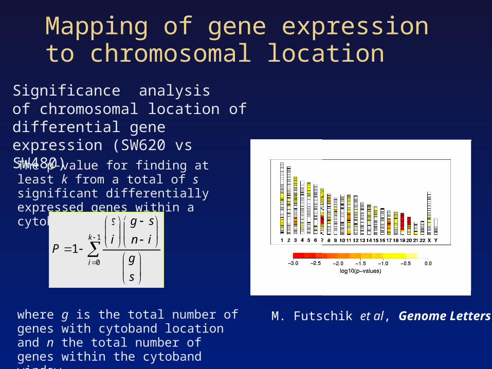
Mapping of gene expression to chromosomal location

Significance analysisof chromosomal location of differential gene expression (SW620 vs SW480)

1

0

1

k

i

s g s

i n iP

g

s

The p-value for finding at least k from a total of s significant differentially expressed genes within a cytoband window is

where g is the total number of genes with cytoband location and n the total number of genes within the cytoband window.

M. Futschik et al, Genome Letters, 2002

Minefield V :There is more than just nuggets and soil

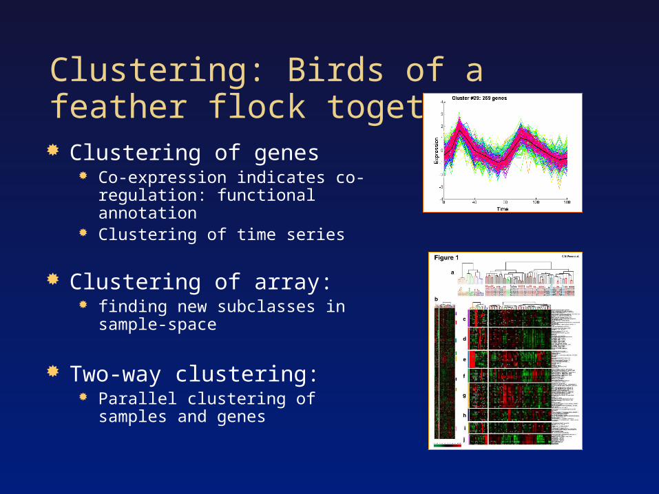
Clustering: Birds of a feather flock together Clustering of genes

Co-expression indicates co-regulation: functional annotation

Clustering of time series

Clustering of array: finding new subclasses in sample-

space

Two-way clustering: Parallel clustering of samples and

genes

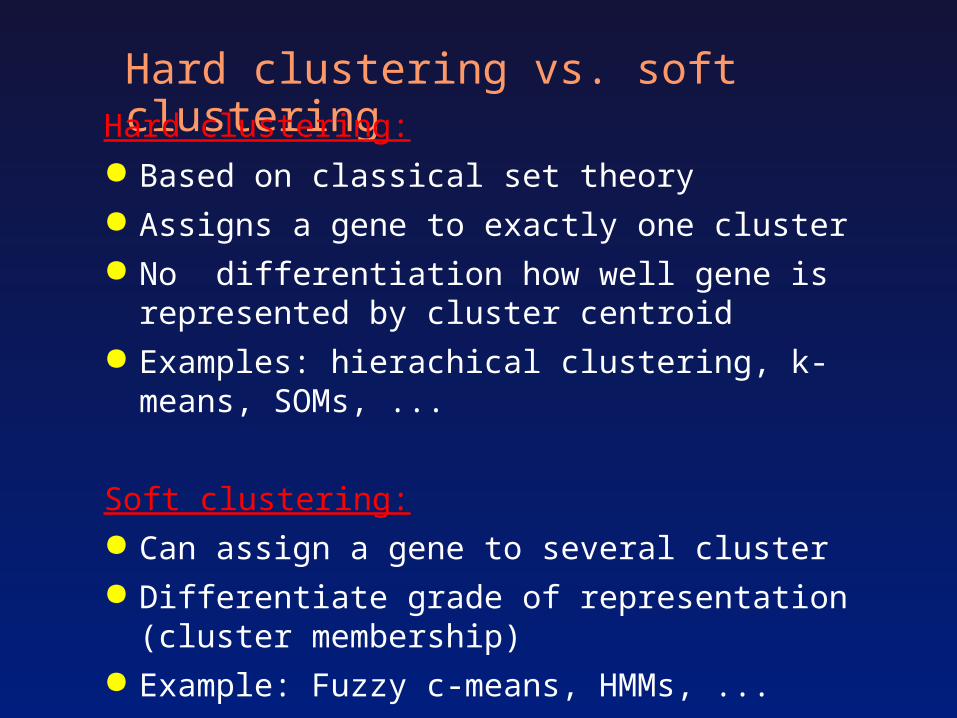
Hard clustering vs. soft clustering

Hard clustering:

● Based on classical set theory● Assigns a gene to exactly one cluster● No differentiation how well gene is represented by

cluster centroid● Examples: hierachical clustering, k-means, SOMs, ...

Soft clustering:● Can assign a gene to several cluster● Differentiate grade of representation (cluster membership)● Example: Fuzzy c-means, HMMs, ...

K-means clustering

1

1

0 1

1

0

ij

kk N

hc ij iji

N

ijj

i j

M U R j

N i

2( ) i ji j

E d x c

Partitional clustering is frequently based on the optimisation of a given objective function. If the data is given as a set of N dimensional vectors, a common objective function is the square error function:

where d is the distance metric and cj is the centre of clusters.

• Partitional clustering splits the data in k partitions with a given integer k. • Partition can represented by a partition matrix U that contains the membership values μij of each object i for each cluster j.• For clustering methods, which is based on classical set theory, clusters are mutually exclusive. This leads to the so called hard partitioning of the data.

Hard partions are defined as

k is the number of clusters and N is the number of data objects.

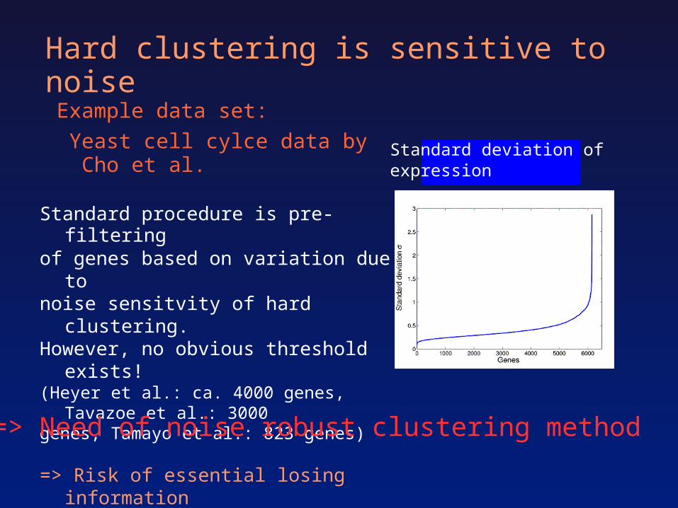
Hard clustering is sensitive to noise

Example data set:

Yeast cell cylce data by Cho et al.

Standard procedure is pre-filteringof genes based on variation due to noise sensitvity of hard clustering.However, no obvious threshold exists!(Heyer et al.: ca. 4000 genes, Tavazoe et al.: 3000genes, Tamayo et al.: 823 genes)

=> Risk of essential losing information

=> Need of noise robust clustering method

Standard deviation of expression

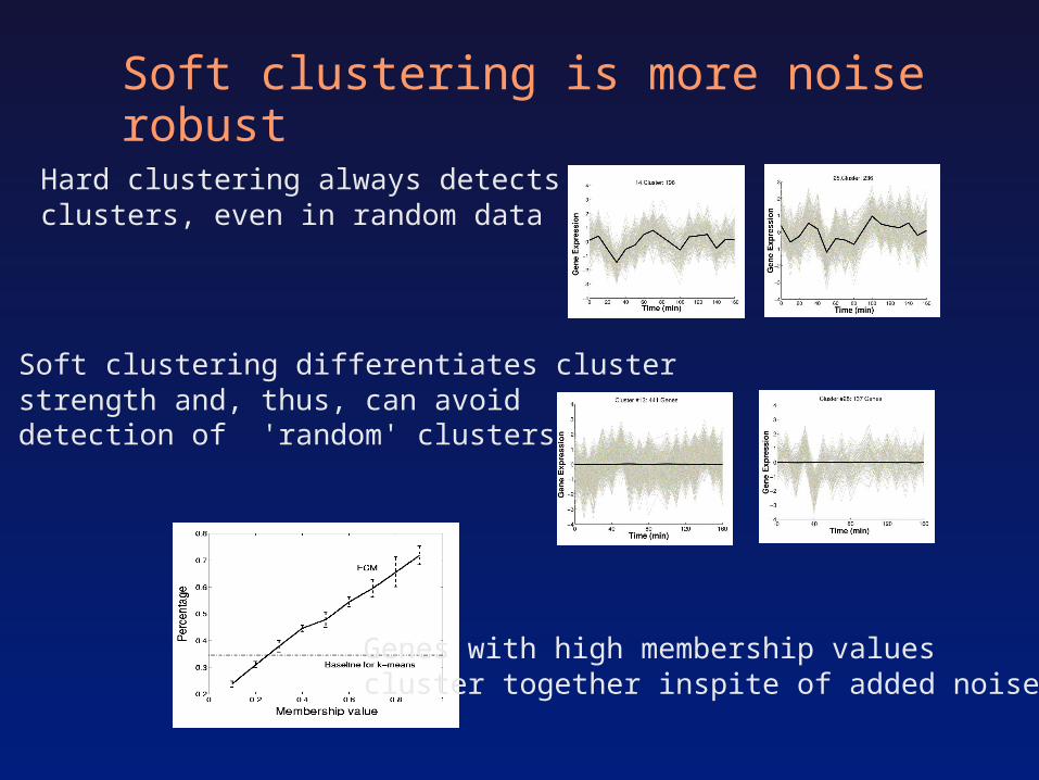
Soft clustering is more noise robust

Hard clustering always detects clusters, even in random data

Soft clustering differentiates clusterstrength and, thus, can avoid detection of 'random' clusters

Genes with high membership valuescluster together inspite of added noise

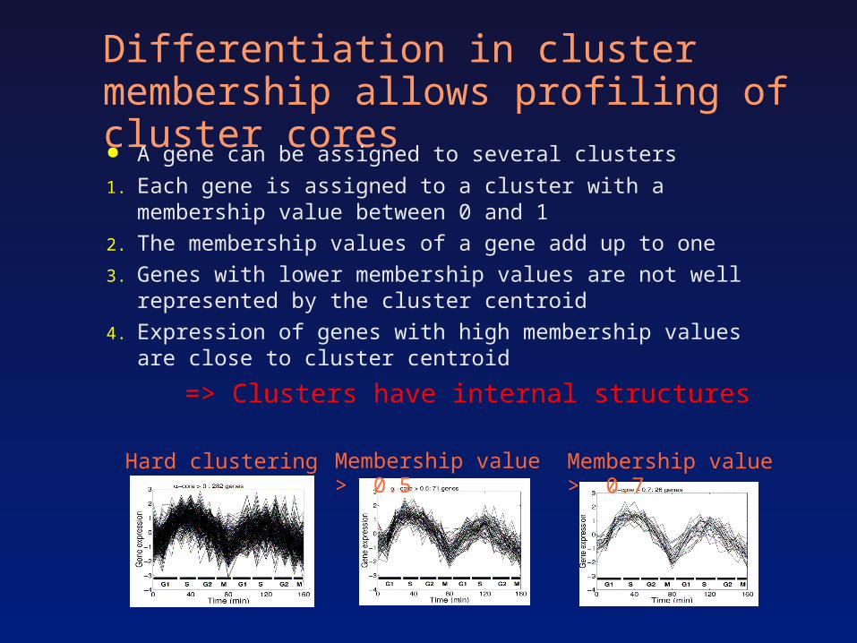
Differentiation in cluster membership allows profiling of cluster cores● A gene can be assigned to several clusters

1. Each gene is assigned to a cluster with a membership value between 0 and 1

2. The membership values of a gene add up to one

3. Genes with lower membership values are not well represented by the cluster centroid

4. Expression of genes with high membership values are close to cluster centroid

=> Clusters have internal structures

Membership value > 0.5 Membership value > 0.7

Hard clustering

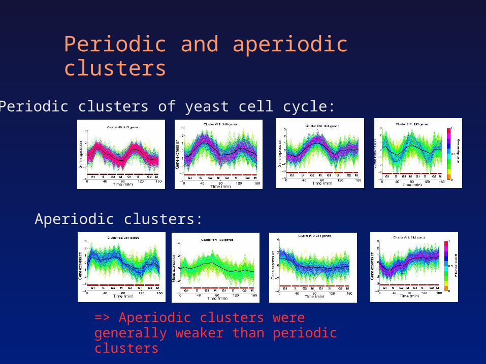
Periodic and aperiodic clusters

Periodic clusters of yeast cell cycle:

Aperiodic clusters:

=> Aperiodic clusters were generally weaker than periodic clusters

Global clustering structure

c-means clustering allows definitionof overlap of clusters i.e. how manygenes are shared by two clusters. This enables to define a similarity measure between clusters. Global clustering structures can be visualised by graphs i.e. edges representing overlap.

Increasing number of clusters

Non-linear 2D-projection by Sammon's Mapping

=> Sub-clustering reveals sub-structures

M. Futschik and B. Carlisle, Noise robust, soft clustering of gene expression data (submitted)

Take-home messages

●There are many mines to step in, so take care of every step●Well begun is half done: A good design of an microarray experiment can avoid a lot of trouble.● A detailed analysis of microarray data can be tedious, but is often worth the effort.●There is still a lot of gold out there....

Thanks!

This talk, the OLIN software and further informationcan be found at http://itb.biologie.hu-berlin.de/~futschik