Embed Size (px)
Citation preview
Microalgae treatment of piggery wastewater
Maria Beatriz Sá Mesquita da Silva Cristóvão
Thesis to obtain the Master of Science Degree in
Biological Engineering
Supervisors: Prof. Valeria Maria Federica Mezzanotte Prof. Nídia Dana Mariano Lourenço de Almeida
Examination Committee
Chairperson: Prof. Jorge Humberto Gomes Leitão
Supervisor: Dra. Nídia Dana Mariano Lourenço de Almeida
Member of the committee: Dra. Maria Teresa Ferreira Cesário Smolders
November, 2016

ii
Acknowledgements
I would like to thank to all the people that has been part of my life during my university experience
in the last 5 years.
A special thanks to my supervisor at Bicocca Valeria Mezzanotte for allowing me to work on this
project, for teaching me and for supporting me in the moments when I was feeling more homesick.
A special thanks to my supervisor at Instituto Superior Técnico Nídia Lourenço for helping me a
lot during the last months of my thesis and for always being available.
Thanks to Giulia Durins for her friendship, for helping me in the laboratory and for performing
some laboratory analyses when I came to Portugal on Easter.
Thanks to Simone Rossi for always being available to help me and for encouraging me in the last
months.
Thanks to Francesca Marazzi, Micol Belucci and prof. Elena Ficara for helping me.
A huge thanks to my family for always believing me, for supporting me whenever I needed and for
all the patience during these last 5 years.
Thanks to my friends: to the old ones and to the new ones that I got the pleasure to meet during
university and also during my Erasmus time in Milan.
Thanks to my flatmates in Milan, Barbara and Guliz, for being my second family, for always being
there for me and for all the good memories of the time that we spent together.
So, thanks to everyone that has crossed in my path over the past 5 intense years.
iii
Abstract
The disposal of untreated or improperly treated wastewater into aquatic environments results in
high nutrient loading into aquatic bodies, which may cause phytoplankton blooms and other environmental
problems. Therefore, in order to discharge these effluents without causing any danger to human´s health or
to natural environmental resources, it is necessary to find the most suitable technique for wastewater
treatment. Recently, several studies have proposed the use of microalgae for wastewater treatment,
highlighting their ability to uptake nutrients, such as phosphorus and nitrogen, and to produce a valuable
biomass, which can be used for biofuels production.
The aim of this thesis was to investigate the efficiency of a microalgae consortium for treating a pre-
treated piggery wastewater by assessing microalgae growth and nutrients removal efficiency, and also to
investigate their ability to produce biogas. Microalgae proved to be able to grow on this high strength
wastewater with high biomass yields and with high nutrients removal efficiency. The highest removal
efficiency of N-NH+4 and P-PO4 was 92 % and 82%, respectively. Moreover, the highest removal efficiency
of COD was 64%, which was partly attributed to the synergetic relationship between microalgae and other
microorganisms. Furthermore, the highest biogas production was 270.4 mLCH4.g-1VS.
For that reason, the hypothesis of using microalgae based treatment as the first step of biological
treatment of piggery wastewater could be considered. In that case, algae biomass could be digested and
the liquid phase of digestate could be recirculated upflow to be treated by algae/bacteria consortium along
with the pre-treated piggery wastewater.
Keywords: Microalgae, Piggery wastewater, Biogas, Nutrients, Removal
iv
Resumo
A descarga de águas residuais não ou inadequadamente tratadas em ambientes aquáticos resulta na
acumulação de nutrientes, os quais podem causar diversos problemas para a saúde humana e para o meio ambiente.
Por conseguinte, a fim de descarregar estes efluentes é necessário encontrar a técnica mais adequada para o
tratamento de águas residuais. Recentemente, vários estudos têm proposto o uso de microalgas no tratamento de
águas devido à sua capacidade de absorção de nutrientes, tais como fósforo e azoto, e de produção de uma biomassa
valiosa, que pode ser utilizada para produzir biocombustíveis.
O objetivo deste trabalho foi investigar a eficiência de um consórcio de microalgas para o tratamento de um
efluente de suinicultura pré-tratado por flotação e investigar a sua capacidade para produzir biogás. As microalgas
utilizadas provaram ser capazes de crescer nestas águas residuais com rendimentos elevados de biomassa e
eficiências elevadas de remoção de nutrientes. A maior eficiência de remoção de N-NH+4 e P-PO4 foi de 92% e 82%,
respetivamente. Além disso, a maior eficiência de remoção de COD foi de 64%, o que confirmou a relação de sinergia
entre microalgas e outros microrganismos. A maior produção de biogás foi 270.4 mLCH4.g-1VS.
Assim, a hipótese de utilizar as microalgas como o primeiro passo de tratamento biológico de águas residuais
de suinicultura pode ser considerado. Nesse caso, a biomassa de algas pode ser digerida e a fase líquida dos digestores
pode ser recirculada e ser tratada pelo consórcio de microalgas/bactérias juntamente com o efluente de suinicultura pré-
trado.
Palavras-chave: Microalgas, Efluente de suinicultura, Biogás, Nutrientes, Remoção
v
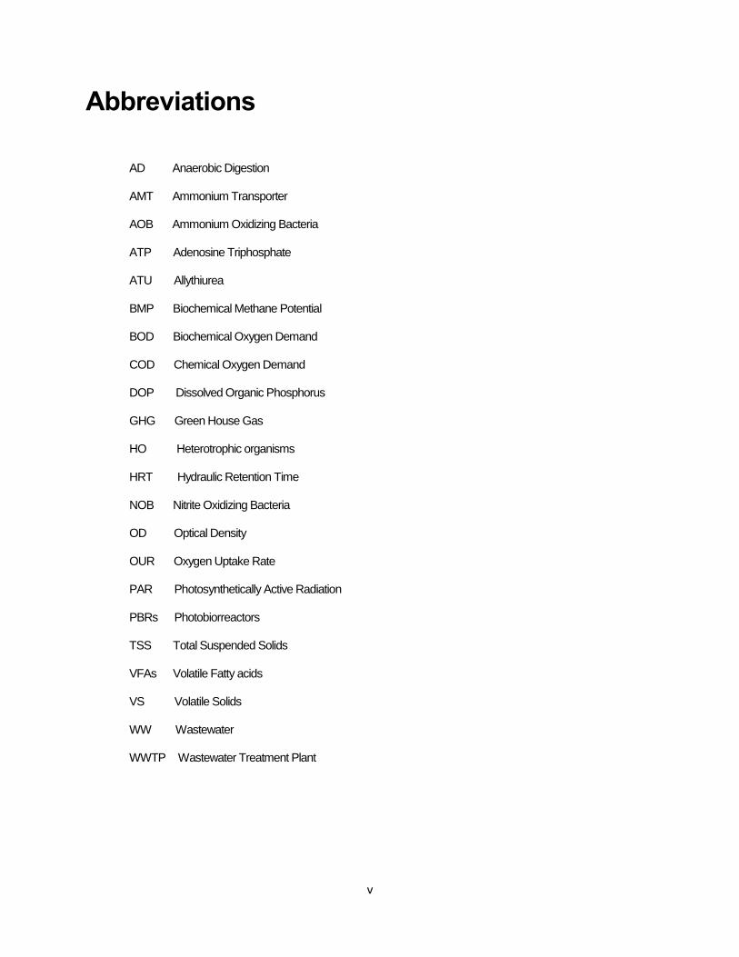
Abbreviations
AD Anaerobic Digestion
AMT Ammonium Transporter
AOB Ammonium Oxidizing Bacteria
ATP Adenosine Triphosphate
ATU Allythiurea
BMP Biochemical Methane Potential
BOD Biochemical Oxygen Demand
COD Chemical Oxygen Demand
DOP Dissolved Organic Phosphorus
GHG Green House Gas
HO Heterotrophic organisms
HRT Hydraulic Retention Time
NOB Nitrite Oxidizing Bacteria
OD Optical Density
OUR Oxygen Uptake Rate
PAR Photosynthetically Active Radiation
PBRs Photobiorreactors
TSS Total Suspended Solids
VFAs Volatile Fatty acids
VS Volatile Solids
WW Wastewater
WWTP Wastewater Treatment Plant
vi
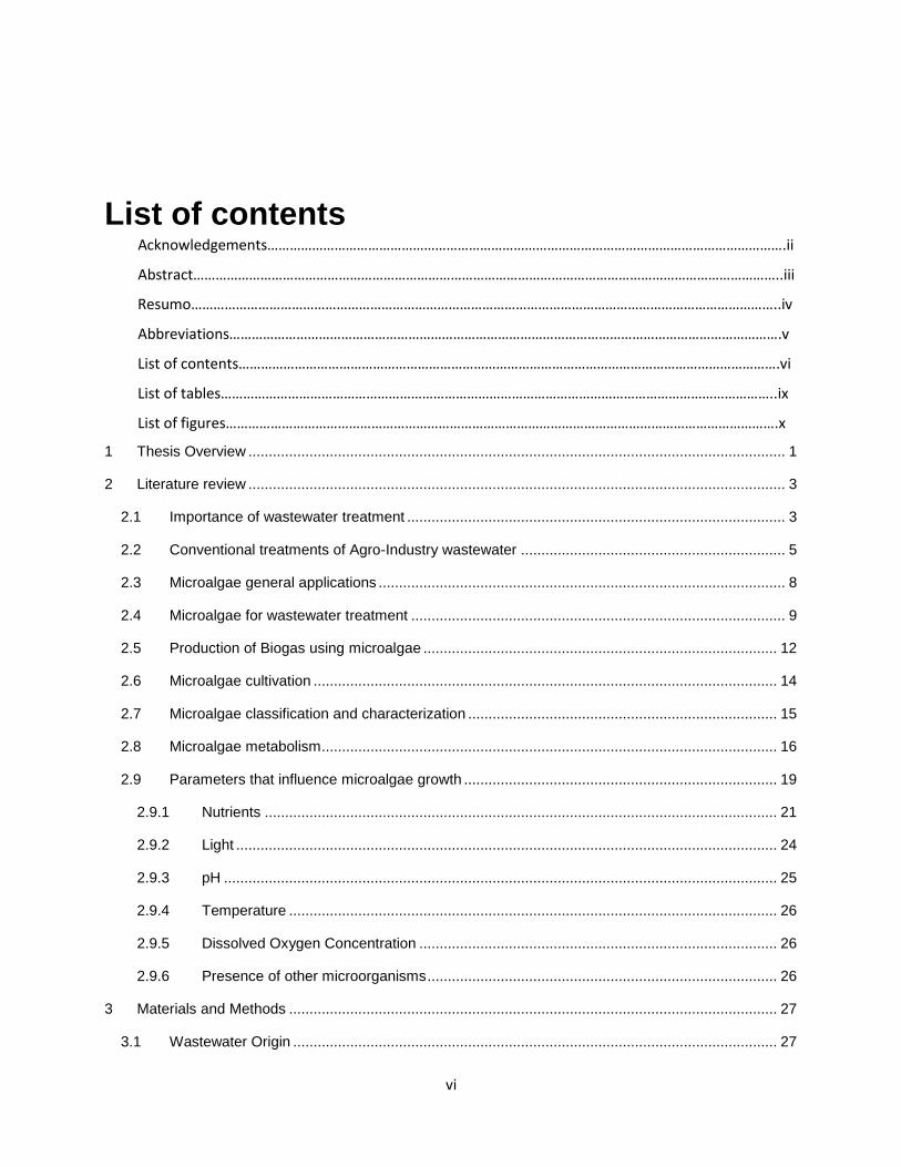
List of contents Acknowledgements………………………………………………………………………………………………………………………….ii
Abstract…………………………………………………………………………………………………………………………………………..iii
Resumo…………………………………………………………………………………………………………………………………………..iv
Abbreviations………………………………………………………………………………………………………………………………….v
List of contents……………………………………………………………………………………………………………………………….vi
List of tables…………………………………………………………………………………………………………………………………..ix
List of figures………………………………………………………………………………………………………………………………….x
1 Thesis Overview .................................................................................................................................... 1
2 Literature review .................................................................................................................................... 3
2.1 Importance of wastewater treatment ............................................................................................. 3
2.2 Conventional treatments of Agro-Industry wastewater ................................................................. 5
2.3 Microalgae general applications .................................................................................................... 8
2.4 Microalgae for wastewater treatment ............................................................................................ 9
2.5 Production of Biogas using microalgae ....................................................................................... 12
2.6 Microalgae cultivation .................................................................................................................. 14
2.7 Microalgae classification and characterization ............................................................................ 15
2.8 Microalgae metabolism ................................................................................................................ 16
2.9 Parameters that influence microalgae growth ............................................................................. 19
2.9.1 Nutrients .............................................................................................................................. 21
2.9.2 Light ..................................................................................................................................... 24
2.9.3 pH ........................................................................................................................................ 25
2.9.4 Temperature ........................................................................................................................ 26
2.9.5 Dissolved Oxygen Concentration ........................................................................................ 26
2.9.6 Presence of other microorganisms ...................................................................................... 26
3 Materials and Methods ........................................................................................................................ 27
3.1 Wastewater Origin ....................................................................................................................... 27
vii
3.2 Microalgae Culture ...................................................................................................................... 28
3.2.1 Experimental plan ................................................................................................................ 29
3.3 Analytical Methods ...................................................................................................................... 30
3.4 Algae growth measurement ......................................................................................................... 31
3.4.1 Optical density ..................................................................................................................... 31
3.4.2 Turbidty ................................................................................................................................ 32
3.4.3 Total suspended solids ........................................................................................................ 32
3.4.4 Microalgae counting ............................................................................................................ 33
3.5 Experimental procedure .............................................................................................................. 34
3.6 Respirometric analysis ................................................................................................................ 35
3.7 BMP tests .................................................................................................................................... 37
4 Results ................................................................................................................................................. 38
4.1 Algae growth parameters ............................................................................................................ 38
4.1.1 Correlation between different parameters ........................................................................... 38
4.1.2 Variation of TSS with time ................................................................................................... 40
4.1.3 Microalgae productivity ........................................................................................................ 41
4.1.4 Microalgae predominance ................................................................................................... 42
4.1.5 Variation of TSS with pH ..................................................................................................... 43
4.1.6 Possible inhibitory effects .................................................................................................... 44
4.2 Treatment efficiency .................................................................................................................... 45
4.2.1 Nitrogen removal ................................................................................................................. 45
4.2.2 Phosphorus removal ............................................................................................................ 49
4.2.3 COD removal ....................................................................................................................... 50
4.3 Respirometry ............................................................................................................................... 51
4.4 BMP ............................................................................................................................................. 52
5 Discussion ........................................................................................................................................... 54
6 Conclusions ......................................................................................................................................... 59
7 Future Perspectives ............................................................................................................................. 61
8 References .......................................................................................................................................... 62

viii
Annexes I……………………………………………………………………………………………………....71
ix
List of tables
Table 3.1 Average parameters of wastewater WW1 and standard deviation ............................................. 28
Table 3.2 Average temperature (°C), pH, conductivity (mS.cm-1) and its standard deviation for vial 1, 2, A
and B ........................................................................................................................................................... 30
Table 3.3 Concentration of the prepared solutions used during respirometric analyses ............................ 36
Table 4.1 Representation of average daily productivity, expressed in g.L-1.day-1, and standard deviation for
each vial....................................................................................................................................................... 41
Table 4.2 Removal efficiencies of N-NH4+ from piggery wastewater by microalgae-bacterial based system
..................................................................................................................................................................... 47
Table 4.3 Nitrogen apportioning, expressed in %, for each vial .................................................................. 49
Table 4.4 Removal efficiencies of P-PO4 from piggery wastewater by microalgae-bacterial based system
..................................................................................................................................................................... 50
Table 4.5 Removal efficiencies of COD from piggery wastewater by microalgae-bacterial based system 50
Table 4.6 Representation of R square and the average oxygen uptake rate, expressed in mg.L-1.h-1, for
the different phases as well as the standard deviation ............................................................................... 52
x
List of figures
Figure 1.1 Linear economy approach versus Circular economy approach (Bradley 2015) .......................... 1
Figure 1.2 Main flows in a conventional WWTP and in an innovative WWTP .............................................. 2
Figure 2.1 Worldwide freshwater sources availability in 2025 (Rekacewicz 2012) ....................................... 3
Figure 2.2 Ratio of treated and untreated wastewater reaching water bodies of 10 regions (Ahlenius 2010)
....................................................................................................................................................................... 4
Figure 2.3 Methane yields (mLCH4.g-1 VS) from different microalgae species (Mezzanotte et al. 2015) ...... 12
Figure 2.4 The dark process of carbon assimilation by photosynthetic microalgae (Chisti et al., 2014) .... 18
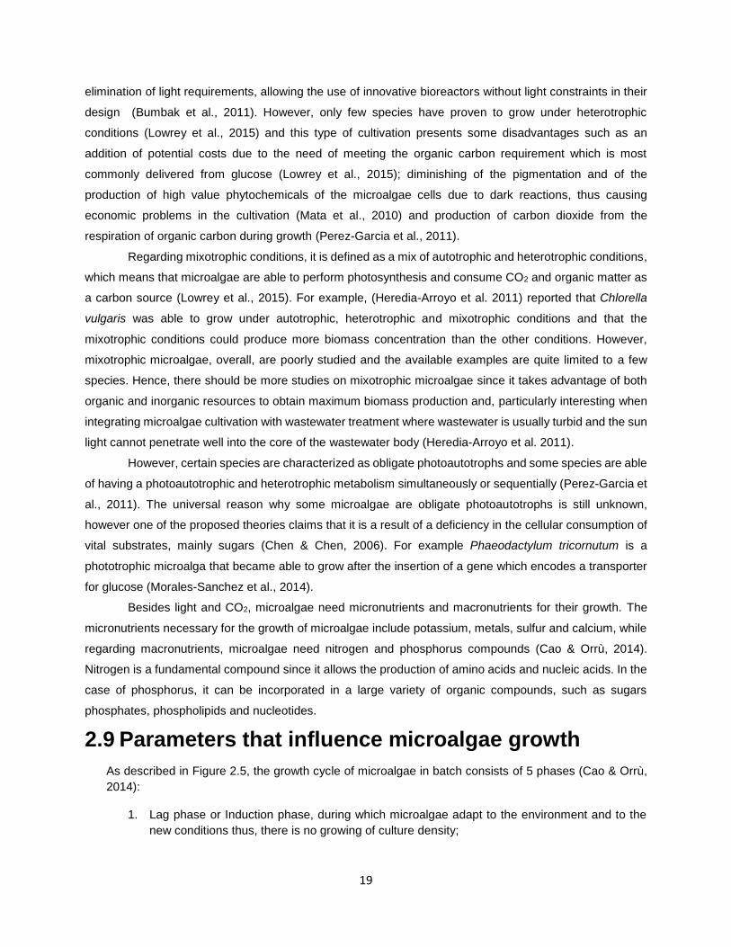
Figure 2.5 Schematic representation of microalgae growth in a batch culture (Cao & Orrù, 2014) ........... 20
Figure 2.6 Effect of light in microalgae growth rate (Yusuf 2007) ............................................................... 24
Figure 3.1 Satellite image of Corte Grande WWTP, in Italy ........................................................................ 27
Figure 3.2 Chlorella spp. (left) (Škaloud 2007) and Scenedesmus spp (right) (Morgan 2005). ................. 28
Figure 3.3 System used for the growth of microalgae cultures ................................................................... 30
Figure 3.4 Kit Hach Lange and Spectrophotometer DR3900 ...................................................................... 31
Figure 3.5 Example of a curve obtained from the measurement of absorbance at different wavelengths . 32
Figure 3.6 One of the two gridded areas (3x 3mm) and a hemocytometer (right bottom) .......................... 33
Figure 3.7 Example of BMP tests performed in the laboratory A.Rozzi, in the Cremona site of Politecnico
di Milano ...................................................................................................................................................... 37
Figure 4.1 Relationship between optical density [-] and turbidity (FAU) for vials 1, 2, A and B…………….38
Figure 4.2 Relationship between optical density [-] and microalgae count (Cell.mL-1) of 9 little squares of the
hemocytometer for vials 1, 2, A and B……………………………………………………………………………38
Figure 4.3 Relationship between OD [-] and microalgae count (cell.mL-1) of 72 squares of the
hemocytometer for vials 1, 2, A and B……………………………………………………………………………..39
Figure 4.4 Relationship between optical density [-] and total suspended solids (g.L-1) for vials 1, 2, A and
B………………………………………………………………………………………………………………………39
Figure 4.5 Variation of total suspended solids, expressed in g.L-1, for the four vials………………………..40
Figure 4.6 Representation of total algae as well as total Chlorella spp. and Scenedesmus spp. expressed
in cell.L-1 for each vial……………………………………………………………………………………………….42
Figure 4.7 Representation of the variation of total suspended solids, expressed in g.L-1, with pH……..........43
Figure 4.8 Variation of TSS, in g.L-1, and unionized ammonia concentration, in mg.L-1, during the
experiments………………………………………………………………………………………………………….44
Figure 4.9 Variation of TSS, in g.L-1, and nitrite concentration, in mg.L-1, during the experiments………...45
Figure4.10 Time course of N-NH4+ concentration in the effluent, expressed in mg.L1………………………46
Figure4.11 Time course of N-NO-2 concentration in the effluent, expressed in mg.L-1……………………….46
Figure 4.12 Time course of N-NO-3 concentration in the effluent, expressed in mg.L1………………………..47
Figure 4.13 Time course of P-PO4 concentration in the effluent, expressed in mg.L-1………………………...49
xi
Figure 4.14 Time course of COD concentration in the effluent, expressed in mgO2.L-1…………………….50
Figure 4.15 Representation of dissolved oxygen concentration, expressed in mg.L-1, during time as well as
oxygen uptake rate (mg.L-1.h-1)…………………………………………………………………………………….51
Figure 4.16 Cumulative biomethane production curves in mLCH4.g-1 VS, over time………………………….52
1
1 Thesis Overview The future of human population and Earth’s capacity are highly unpredictable since they depend on
both natural limitations and human behavior. Recent studies proposed that, although the growth rate of the
world population appears to be decreasing, the total number of humans on Earth is estimated to rise by
50% during this century, reaching 11 billion of people (Ortiz-Ospina & Roser 2016) .This means that the
world population will need to find more and more resources such as food, water, raw materials and energy
in a world where they look already scarce and where our environmental impact is damaging the planet. The
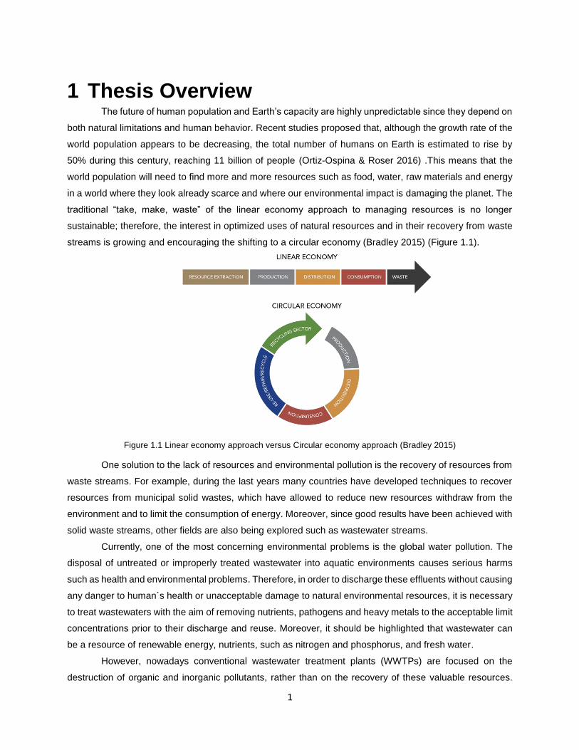
traditional “take, make, waste” of the linear economy approach to managing resources is no longer
sustainable; therefore, the interest in optimized uses of natural resources and in their recovery from waste
streams is growing and encouraging the shifting to a circular economy (Bradley 2015) (Figure 1.1).
Figure 1.1 Linear economy approach versus Circular economy approach (Bradley 2015)
One solution to the lack of resources and environmental pollution is the recovery of resources from
waste streams. For example, during the last years many countries have developed techniques to recover
resources from municipal solid wastes, which have allowed to reduce new resources withdraw from the
environment and to limit the consumption of energy. Moreover, since good results have been achieved with
solid waste streams, other fields are also being explored such as wastewater streams.
Currently, one of the most concerning environmental problems is the global water pollution. The
disposal of untreated or improperly treated wastewater into aquatic environments causes serious harms
such as health and environmental problems. Therefore, in order to discharge these effluents without causing
any danger to human´s health or unacceptable damage to natural environmental resources, it is necessary
to treat wastewaters with the aim of removing nutrients, pathogens and heavy metals to the acceptable limit
concentrations prior to their discharge and reuse. Moreover, it should be highlighted that wastewater can
be a resource of renewable energy, nutrients, such as nitrogen and phosphorus, and fresh water.
However, nowadays conventional wastewater treatment plants (WWTPs) are focused on the
destruction of organic and inorganic pollutants, rather than on the recovery of these valuable resources.
2
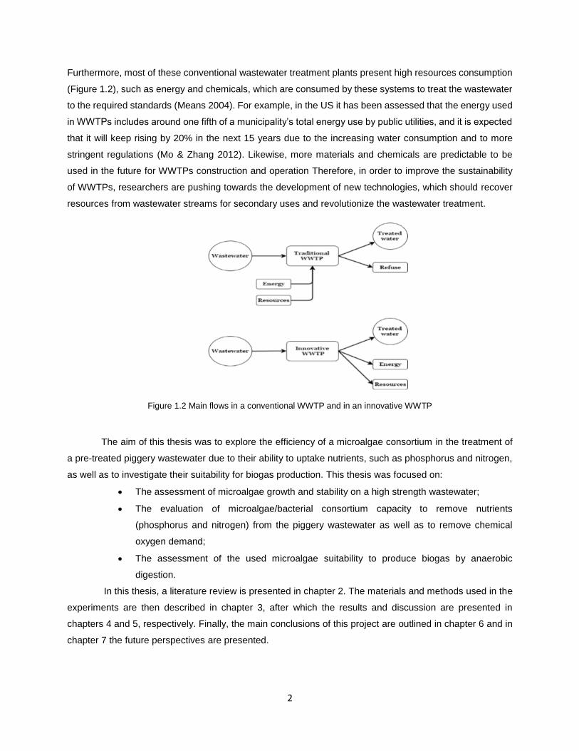
Furthermore, most of these conventional wastewater treatment plants present high resources consumption
(Figure 1.2), such as energy and chemicals, which are consumed by these systems to treat the wastewater
to the required standards (Means 2004). For example, in the US it has been assessed that the energy used
in WWTPs includes around one fifth of a municipality’s total energy use by public utilities, and it is expected
that it will keep rising by 20% in the next 15 years due to the increasing water consumption and to more
stringent regulations (Mo & Zhang 2012). Likewise, more materials and chemicals are predictable to be
used in the future for WWTPs construction and operation Therefore, in order to improve the sustainability
of WWTPs, researchers are pushing towards the development of new technologies, which should recover
resources from wastewater streams for secondary uses and revolutionize the wastewater treatment.
Figure 1.2 Main flows in a conventional WWTP and in an innovative WWTP
The aim of this thesis was to explore the efficiency of a microalgae consortium in the treatment of
a pre-treated piggery wastewater due to their ability to uptake nutrients, such as phosphorus and nitrogen,
as well as to investigate their suitability for biogas production. This thesis was focused on:
The assessment of microalgae growth and stability on a high strength wastewater;
The evaluation of microalgae/bacterial consortium capacity to remove nutrients
(phosphorus and nitrogen) from the piggery wastewater as well as to remove chemical
oxygen demand;
The assessment of the used microalgae suitability to produce biogas by anaerobic
digestion.
In this thesis, a literature review is presented in chapter 2. The materials and methods used in the
experiments are then described in chapter 3, after which the results and discussion are presented in
chapters 4 and 5, respectively. Finally, the main conclusions of this project are outlined in chapter 6 and in
chapter 7 the future perspectives are presented.
3
2 Literature review
2.1 Importance of wastewater treatment
At present, it is universally recognized that fresh water and sustainable water management is one
of the most important concerns of innumerous scientific, social or political groups. However, water resources
seem to face severe quantitative and qualitative threats, since pollution and population growth,
industrialization and rapid economic development inflict severe risks to the availability and quality of water
resources in many worldwide areas (Abdel-Raouf et al. 2012).
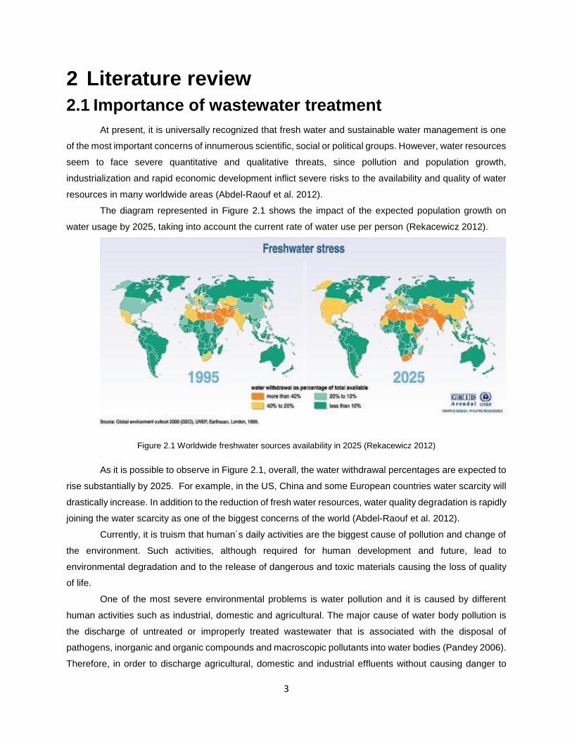
The diagram represented in Figure 2.1 shows the impact of the expected population growth on
water usage by 2025, taking into account the current rate of water use per person (Rekacewicz 2012).
Figure 2.1 Worldwide freshwater sources availability in 2025 (Rekacewicz 2012)
As it is possible to observe in Figure 2.1, overall, the water withdrawal percentages are expected to
rise substantially by 2025. For example, in the US, China and some European countries water scarcity will
drastically increase. In addition to the reduction of fresh water resources, water quality degradation is rapidly
joining the water scarcity as one of the biggest concerns of the world (Abdel-Raouf et al. 2012).
Currently, it is truism that human´s daily activities are the biggest cause of pollution and change of
the environment. Such activities, although required for human development and future, lead to
environmental degradation and to the release of dangerous and toxic materials causing the loss of quality
of life.
One of the most severe environmental problems is water pollution and it is caused by different
human activities such as industrial, domestic and agricultural. The major cause of water body pollution is
the discharge of untreated or improperly treated wastewater that is associated with the disposal of
pathogens, inorganic and organic compounds and macroscopic pollutants into water bodies (Pandey 2006).
Therefore, in order to discharge agricultural, domestic and industrial effluents without causing danger to
4
human health or unacceptable damage to the natural environment resources, it is necessary to treat
wastewaters with the aim of removing nutrients, pathogens and heavy metals to the acceptable limit
concentrations prior to their discharge and reuse (Abdel-Raouf et al. 2012).
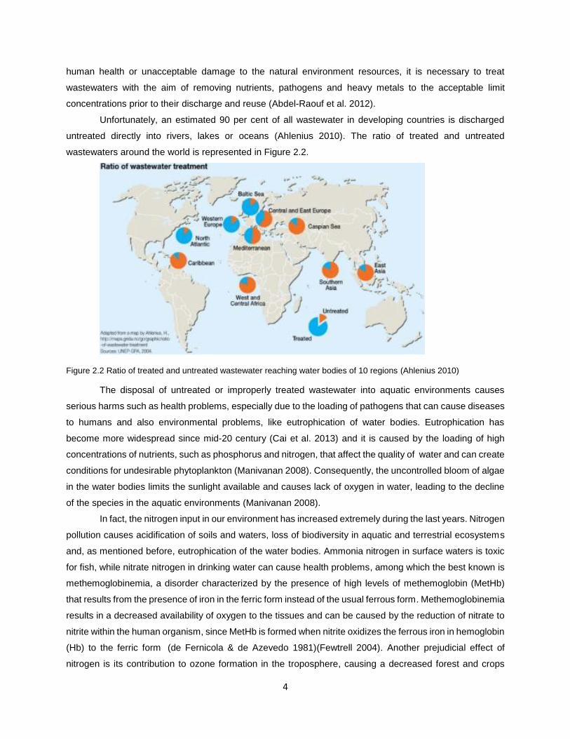
Unfortunately, an estimated 90 per cent of all wastewater in developing countries is discharged
untreated directly into rivers, lakes or oceans (Ahlenius 2010). The ratio of treated and untreated
wastewaters around the world is represented in Figure 2.2.
Figure 2.2 Ratio of treated and untreated wastewater reaching water bodies of 10 regions (Ahlenius 2010)
The disposal of untreated or improperly treated wastewater into aquatic environments causes
serious harms such as health problems, especially due to the loading of pathogens that can cause diseases
to humans and also environmental problems, like eutrophication of water bodies. Eutrophication has
become more widespread since mid-20 century (Cai et al. 2013) and it is caused by the loading of high
concentrations of nutrients, such as phosphorus and nitrogen, that affect the quality of water and can create
conditions for undesirable phytoplankton (Manivanan 2008). Consequently, the uncontrolled bloom of algae
in the water bodies limits the sunlight available and causes lack of oxygen in water, leading to the decline
of the species in the aquatic environments (Manivanan 2008).
In fact, the nitrogen input in our environment has increased extremely during the last years. Nitrogen
pollution causes acidification of soils and waters, loss of biodiversity in aquatic and terrestrial ecosystems
and, as mentioned before, eutrophication of the water bodies. Ammonia nitrogen in surface waters is toxic
for fish, while nitrate nitrogen in drinking water can cause health problems, among which the best known is
methemoglobinemia, a disorder characterized by the presence of high levels of methemoglobin (MetHb)
that results from the presence of iron in the ferric form instead of the usual ferrous form. Methemoglobinemia
results in a decreased availability of oxygen to the tissues and can be caused by the reduction of nitrate to
nitrite within the human organism, since MetHb is formed when nitrite oxidizes the ferrous iron in hemoglobin
(Hb) to the ferric form (de Fernicola & de Azevedo 1981)(Fewtrell 2004). Another prejudicial effect of
nitrogen is its contribution to ozone formation in the troposphere, causing a decreased forest and crops
5
production as well as human’s health problems. Additionally, nitrogen in the form of ammonia can be
released to the atmosphere contributing to the formation of acid rains.
Wastewater treatment methods are generally classified in three types: biological, chemical and
physical. These methods can be applied individually or in combination, depending on the nature and type
of pollution. Usually, physical and chemical methods are costly and chemical methods are normally
associated with the increase of conductivity, pH and overall load of dissolved matter in the wastewater
(Renuka et al. 2015). Therefore, biological treatment methods tend to be much more promising.
Agricultural wastewater, which is mainly obtained from livestock productions, is one of the biggest
contributors to nitrogen discharge since it has high concentrations of ammonium (Lim et al. 2016). For years,
the traditional method to treat piggery wastewater was using it as a fertilizer for lands, but the nitrogen in
piggery wastewater cannot be completely uptaken by crops due to the unbalanced N/P ratio (Cai et al.
2013). The consequent accumulation of nitrogen in the soil can contaminate the receiving waters and cause
all the problems previously described.
Therefore, it is important to find the most cost-effective and environmentally friendly treatment
methods that require less inputs and simple infrastructures to treat piggery wastewater.
2.2 Conventional treatments of Agro-Industry
wastewater
Livestock production started to raise during the end of 20th century (Hjorth et al. 2010) and,
nowadays, the increased demand for red meat in developing countries has led to the intensification of
livestock production and consequently, to the development of large indoor animal houses, mainly pigs and
poultry,(Bernet & Béline 2009), resulting in higher local emissions of odor and ammonia gas (Hjorth et al.
2010). In addition, the intensification of livestock production has led to the concentration of animals in limited
areas with the aim of reducing production costs (Bernet & Béline 2009). In these areas, the local use of
wastewater as organic fertilizer results in over-application of nutrients on soils, causing several
environmental problems. For example, in Brittany (France) before the intensification of livestock production
the average concentration of NO-3 in a surface water used to be 5 mg.L-1, but nowadays the concentration
has reached the value of 35 mg.L-1 (Bernet & Béline 2009).
For many years, the use of swine manure as organic fertilizer used to be one of the most economical
and easiest methods of managing manure (Lim et al. 2016). However, as mentioned before, there are
several environmental concerns related to over-application of animal manure, including a great risk of
nutrient runoff, which will contaminate surface and ground water; eutrophication of surface waters; spread
of pathogens; attraction of rodents, insects and other pests; and a potential higher energy used in the
transport of manure to the cultivation crops (Iregbu et al. 2014) (Hjorth et al. 2010). Therefore, the use of
manure as fertilizer should be limited and it is necessary to develop a cost-efficient piggery wastewater
treatment, as an alternative to land application.
6
Animal wastewaters may have variable characteristics, depending not only on the different types of
animals, but also for the same animals between countries and farms, depending on the water consumption,
farm production and also, on the composition of the feed given to the animals (Boursier et al. 2005).
Generally, piggery wastewater consists on a mix of urine, manure and flushing wastewater, which is
characterized for having high concentrations of nitrogen, phosphorus, chemical oxygen demand (COD) and
total suspended solids (TSS) (Girard et al. 2009). Many studies have been focused on the biological
removal of carbon, nitrogen and phosphorus, however, few of these studies were carried out on wastewaters
with high concentrations of these compounds, such as piggery wastewater.
Regarding the conventional treatment, firstly it is necessary to perform a preliminary treatment to
remove large solid materials that can damage the downstream equipment and obstruct the flow. These
large solids can be removed by passing the sewage through bars spaced at 20-60 mm (Abdel-Raouf et al.
2012).
After the removal of the coarse solids, sewage may be subjected to a primary treatment which
consists in passing the sewage through sedimentation tanks with the aim of removing the settable solids by
gravity (Abdel-Raouf et al. 2012). Moreover, it should be pointed out that a well design sedimentation tank
can remove almost 40 % of the total COD (Abdel-Raouf et al. 2012).
Then, the secondary treatment process aims to reduce COD by reducing organic compounds and
this is mediated by a mixed population of heterotrophic bacteria that use organic matter for energy and
growth (Abdel-Raouf et al. 2012). Anaerobic digestion (AD) is one of the most frequently used methods for
piggery wastewater due to its reliability, low cost and high efficiency (Wu et al. 2015) (Obaja et al. 2003)
(Chynoweth et al., 1999). This process is defined as the decomposition of biodegradable material by
microorganisms in the absence of oxygen and includes four phases. The first phase, named as hydrolysis,
involves the decomposing of complex molecular organic compounds, such as proteins, fats and
carbohydrates into smaller molecules by anaerobic bacteria using extra-cellular enzymes. Then, in the
second phase, acid forming bacteria continue the degradation of the smaller compounds into carbon
dioxide, organic acids, hydrogen sulfide and ammonia. After that, acetogenesis takes place, leading to the
formation of CO2, acetate and H2 by acetogenic bacteria. Finally, methane forming bacteria produce biogas,
chiefly made of methane and CO2 (methanogenesis).
It is important to point out that anaerobic digestion may be operated in simple systems, such as
anaerobic open ponds, or in closed systems, which are a very efficient way to decrease greenhouse gas
(GHG) emissions into the atmosphere, allowing the production of renewable energy (methane) and
avoiding the uncontrolled emission of GHG produced during animal manure management (Bernet & Béline
2009).
Generally, AD is operated in mesophilic conditions (35-40°C) (Chynoweth et al. 1999). As an
alternative, it can be operated in thermophilic conditions, which benefits from having increased rates and
higher sanitizing effects. However, thermophilic AD is less stable, due to volatile fatty acids (VFAs)
accumulation, and more sensible to potential inhibitors, such as ammonia (Bernet & Béline 2009). Finally,
7
AD can be operated in psychrophilic conditions, at 20°C or less, but the rates are much lower than in
mesophilic or thermophilic conditions (Masse et al. 1997).
Anaerobic digestion has been used for many years for the treatment of organic material in manure
and the biogas produced, mainly composed of CH4 (55-80%) and CO2 (20-45%), can be used for energy
production, as heat or for conversion into electricity (Bernet & Béline 2009). The liquid effluent that is
obtained from the anaerobic digestion, named as digestate, has still high concentrations of nitrogen and
thus needs to be further treated.
The removal of nitrogen is becoming one of the major steps in wastewater treatment plants since
the discharge of its compounds in the water bodies causes important environmental problems, as previously
described. The conventional digestate treatment is based on biological processes that include suspended
and/or biofilm growth systems carrying out nitrification and denitrification (Obaja et al. 2003).
All the biological systems used to remove nitrogen compounds comprise an aerobic phase, where
nitrification occurs, and an anoxic phase allowing denitrification.
The nitrification occurs in two steps, namely the conversion of ammonium to nitrite and the
conversion of nitrite to nitrate. In the first step, chemo-autotrophic ammonium oxidizing bacteria, also known
as AOB (ammonium oxidizing bacteria), convert ammonium to nitrite. Then, in a second step, another type
of chemo-autotrophic bacteria, NOB (nitrite oxidizing bacteria) oxidize nitrite to nitrate.
The autotrophic bacteria responsible for nitrification, discovered in 1891 by Winogradsky (Tilley
2011), belong chiefly to the genera Nitrosomonas (ammonium oxidizer), Nitrospira (nitrite oxidizer) and
Nitrobacter (nitrite oxidizer). These bacteria are chemoautotrophs and produce the energy they need to
grow by oxidizing ammonia or nitrite. Thus, they require and consume oxygen and use CO2 as carbon
source for growing
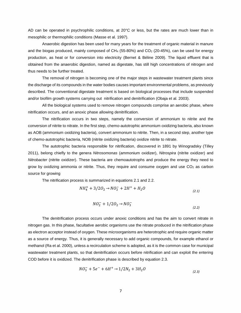
The nitrification process is summarized in equations 2.1 and 2.2.
𝑁𝐻4+ + 3/2𝑂2→𝑁𝑂2
− + 2𝐻+ +𝐻2𝑂
(2.1)
𝑁𝑂2− + 1/2𝑂2→𝑁𝑂3
−
(2.2)
The denitrification process occurs under anoxic conditions and has the aim to convert nitrate in
nitrogen gas. In this phase, facultative aerobic organisms use the nitrate produced in the nitrification phase
as electron acceptor instead of oxygen. These microorganisms are heterotrophic and require organic matter
as a source of energy. Thus, it is generally necessary to add organic compounds, for example ethanol or
methanol (Ra et al. 2000), unless a recirculation scheme is adopted, as it is the common case for municipal
wastewater treatment plants, so that denitrification occurs before nitrification and can exploit the entering
COD before it is oxidized. The denitrification phase is described by equation 2.3.
𝑁𝑂3− + 5𝑒− + 6𝐻+→1/2𝑁2 + 3𝐻2𝑂
(2.3)
8
Most conventional wastewater treatment technologies are not economical for the treatment of
agricultural wastewater, so it is compulsory to find alternative techniques. Microalgae based processes have
been considered a promising biological treatment as microalgae remove nitrogen in one step together with
various kinds of potentially toxic or hazardous pollutants from different types of wastewaters.
2.3 Microalgae general applications
Since the 1950s, researchers have focused on studying the use of microalgae to produce many
important products in a wide range of processes, such as conventional industries, wastewater treatment
and renewable energy production (Bux 2013). Microalgae biomass is mainly cultivated to obtain products
with a commercial interest that are mostly used for animal and human nutrition, cosmetics and
pharmaceuticals.
Since ancient times, microalgae have been widely used in many populations, mainly in Asiatic countries
such as China, Japan and Korea. These organisms contain substances with very interesting antioxidant
properties and are rich in proteins as well as in polyunsaturated fatty acids of the omega- 3 series, vitamins
A, B, C, E, K and B12, potassium, magnesium and other minerals (Priyadarshani & Rath 2012). Being such
a rich source of essential nutrients, they are considered a valuable dietary supplement for humans and
animals (Bux 2013). Depending on the species, the extractable chemical compounds may be different and,
currently, the production of microalgae for human consumption is widely increasing, and different species
have been cultivated to obtain different natural compounds (Herrero et al. 2006).
During the 2000s, several cosmetic companies in Europe and the US start to launch cosmetics that use
extracts from microalgae species, such as Chlorella and Spirulina, (Se-Kwon 2015) since they are able to
produce important compounds that can be used as thickening agents, water binding agents and antioxidants
(Priyadarshani & Rath 2012).
Regarding the pharmaceutical area, it has also been proven that microalgae are rich in biologically
active compounds that present anticancer, antiviral, antifungal and antibacterial properties (Priyadarshani
& Rath 2012). In addition, microalgae have the capacity to produce toxins that may have pharmaceutical
applications (Se-Kwon 2015).
Summing up, depending on the different microalgae species, it is possible to extract diverse valuable
compounds from microalgae biomass, such as fats, polyunsaturated fatty acids, sugars, oils, antioxidants,
enzymes, esters, vitamins, pigments, carotenoids and chlorophyll (Bux 2013). Due to this diversity of high-
value biological derivatives with many commercial applications, microalgae production is currently becoming
much more promising in the area of nutrition and food additives, pharmaceuticals, cosmetics and
aquaculture (as food for aquatic organisms) and, if grown on wastewater, they can also be used as a source
of biofuels and for pollutant removal (Se-Kwon 2015). However, one major constraint to the use of
microalgae is the difficulty in biomass harvesting due to their microscopic size, typically in the 2-40 µm range
and also due to their low cell density, typically in the 0.3-5 g L-1 range (Brennan & Owende 2010).
9
2.4 Microalgae for wastewater treatment
In 1957, Oswald and Gotaas suggested for the first time the use of microalgae for wastewater treatment
(Ruiz-Martinez et al. 2012) due to their photosynthetic capability, converting solar energy into valuable
biomass, and to their capacity to incorporate nutrients like phosphorus and nitrogen. Since then, there have
been several studies using microalgae systems to treat human sewage, livestock wastes, agro-industry
wastes, industrial wastes and also other types of wastes such as piggery effluents and effluents resulting
from food processing factories (Cai et al. 2013).
As an alternative to the conventional wastewater treatment methods, microalgae have proven to be
efficient in removing nitrogen and phosphorus from wastewater and the algae based treatment process is
named as phycoremediation (Renuka et al. 2015). The impact of microalgae wastewater treatment over
conventional treatment must be evaluated in terms of energy and economic factors involved in the operation
process. For example, the oxygen produced during the microalgae photosynthetic process can reduce the
cost deriving from the need for artificial aeration and can limit the risk of pollutant volatilization. Moreover,
wastewater normally sustain a mixed algae/bacteria consortium and the synergy between bacterial and
algal biomass increases the process efficiency (Muñoz & Guieysse 2006).
Besides nutrient removal, phycoremediation involves the removal of BOD, of coliform bacteria, of toxic
metals, like lead, cadmium, arsenic, mercury, bromine and scandium, of xenobiotic compounds and the
sequestration of CO2 (Renuka et al. 2015).
Microalgae enhance the removal of organic pollutants since they furnish O2 to heterotrophic aerobic
bacteria, which are responsible for mineralizing organic compounds, and in return, these bacteria release
CO2, which is used by microalgae for photosynthesis, thus establishing a symbiotic relation (Muñoz &
Guieysse 2006). A limitation of this combined system is linked to the different speed of growth of microalgae
and bacteria, which may reduce the benefits of oxygen production, at least in the starting phase, since the
microalgae growth is slower, consequently it does not provide immediately the necessary oxygen for
bacteria (Mezzanotte et al. 2015). In addition, microalgae can have a negative effect on the microbial
community, as altering the pH and the temperature and they can also produce extracellular metabolites that
may inhibit bacterial growth (Ruiz-Marin et al. 2010).
Another positive aspect due to the synergetic relation between microalgae and bacteria is the fact
that wastewater may contain potentially hazardous and toxic substances for microalgae, such as polycyclic
aromatic hydrocarbons, phenols or organic solvents, but their removal/conversion by bacteria allows
microalgae to adapt to the growth substrate (Brennan & Owende 2010).
Regarding the removal of heavy metals, the most studied microbial biotreament is performed by using
sulfate reducing bacteria, which remove the metals with the production of metal-sulfide precipitates.
However, this treatment has some disadvantages including long residence times (weeks) and the need for
continuous substrate supply (Perales-Vela et al. 2006). On the other hand, microalgae have proven to be
efficient in removing heavy metals, such as zinc, cadmium, mercury, iron and nickel (Renuka et al. 2015)
10
with a specific metal uptake of 15 mg.g-1biomass at 99% removal efficiency, showing that they can be
competitive when compared with the other treatments (Muñoz & Guieysse 2006).
These metals are mainly removed by adsorption/diffusion or surface binding, which is facilitated by the
properties of the algae cell walls (Rawat et al. 2016). The algal cell wall presents chemical affinity to metals
as a result of the presence of several functional groups, such as carboxyl, carbonyl, amido, amino,
sulfhydryl, hydroxyl, which gives negative charge to the cell surface, thus facilitating surface binding with
positively charged metal ions by physical adsorption or chemical processes, including ion exchange,
chelation with covalent bonds and precipitation (De Philippis et al. 2011). In fact, microalgae are able to
release extracellular metabolites that have the capacity of chelating metal ions (Rawat et al. 2016) and the
increase in pH due to photosynthesis may cause the precipitation of heavy metals (Mezzanotte et al. 2015).
The fast growing concern about the global warming, mainly caused by the increase of the CO2 level in
the atmosphere, made the United Nations to promote the protocol Kyoto (1997) with the aim of imposing
the countries all over the world to reduce the greenhouse gas emissions, and more than 170 countries have
ratified the protocol (Wang et al. 2008). Therefore, in the last decade several researches have been
developed in order to find the most suitable techniques to reduce CO2 in the atmosphere. Microalgae have
proven to be promising in this field, since they can sequestrate CO2 from the atmosphere or industrial
exhausted gas, contributing to the reduction of GHG (Renuka et al., 2015) and also to the production of a
valuable biomass that can be applied in the production of useful compounds such as biofuels and fertilizers
(Pires et al. 2012).
Biological mitigation of CO2 can be carried out by terrestrial plants and photosynthetic microorganisms.
However, since microalgae have a simple structure, they have much higher growth rates and CO2 fixation
capacities when compared to conventional aquatic, agricultural and forestry plants, with an efficiency 50
times higher than the terrestrial plants (Li et al. 2008). On average, the production of 1kg of microalgae
biomass involves the consumption of 1.8 kg of CO2 (Chisti 2007).
Many studies on flue gas tolerance by microalgae concluded that some microalgae species can tolerate
high concentrations of CO2, but the levels of SOX and NOX can be a concern since they can inhibit
microalgae growth (Lara-Gil et al. 2014). However, levels of SOx and NOx, up to 150 ppm can also be well
tolerated by some microalgae species (Wang et al. 2008). The most suitable species in the fixation of CO2
seem to belong to Chlorella and Scenedesmus genera (de Morais & Costa 2007).
Finally, the microalgae biomass produced during wastewater treatment can be used for the production
of biofuels. The interest in the use of microalgae for renewable energy started growing in the 1970s during
the first oil crisis (Spolaore et al. 2006) and in the last years the research in microalgae has become more
extensive due to the depletion of fossil fuels and to the global increase of industrial activities, which are
associated to a great need to balance the energy demand and the reduction of greenhouse gas emissions
(Mata et al. 2010).
One of the main interests of using microalgae in the energy sector is due to the fact that they have a
high lipid content and to the wide range of bioenergy products that can be obtained from culturing microalgae
feed-stocks, including biomass for combustion to produce heat and electricity, fermentable sugars to
11
produce bioethanol, biobutanol or biogas, oil for conversion to biodiesel or even possibly algae
biosynthesized biodiesel.
As an alternative to other biofuel sources, microalgae present many advantages such as their fast
growth and short life cycle when compared to terrestrial plants (Sivakumar et al. 2016). For example, the
average value of the maximum specific growth rate of microalgae species is nearly 1 day-1, while for higher
plants it is 0.1 day-1 (Chisti 2010). Additionally, in spite of being aquatic microorganisms, microalgae require
less water than the terrestrial plant crops and since they can grow in harsher conditions and with less
nutrients, they can be cultured in non-arable land, thus not competing for land with food crops (Sivakumar
et al. 2016). Microalgae do not need freshwater for their growth, and consequently they can use different
wastewaters as a growth medium, with no need for chemicals such as herbicides and pesticides (Brennan
& Owende 2010).
Conventional wastewater treatment plants are mainly designed to remove organic compounds by
anaerobic or aerobic biological processes, but the treated effluents still contain residual inorganic
compounds such as nitrate, ammonium and phosphorus, as well as organic compounds quantified by COD
and BOD5. Thus, a tertiary treatment is often required before discharge (Rawat et al. 2016). Microalgae
culturing can be a cost-effective option to remove nutrients from biologically treated effluents, acting as a
tertiary treatment (Abdel-Raouf et al. 2012)(Cai et al. 2013). However, the potential to uptake nutrients
varies among different species (Boelee et al. 2011) and also as a function of some environmental factors
such as light and temperature (Cao & Orrù 2014).
Regarding piggery wastewater, many studies have been conducted in laboratory scale using
microalgae as a tertiary treatment and assessing its potential to treat the liquid digestate obtained from
anaerobic digestion (Uggetti et al. 2014)(Monlau et al. 2015) (Xu et al. 2015), which is the main conventional
process used for removing organic compounds in these types of wastewater. The substances fed to the
digester which cannot be converted into biogas are extracted as digestate, which consists of a mixture of
undegraded organic and inorganic compounds, including heavy metals and nutrients. Particularly, the
organic nitrogen and phosphorous present in the digester feed are found in the digestate mainly in
mineralized form. AD offers two interesting products for the cultivation of microalgae, the off-gas that has a
high content in CO2 and the digestate, which contains high concentrations of nutrients, such as phosphorus
and nitrogen. Therefore, it is interesting to consider the implementation of microalgae cultivation at
anaerobic digestion plants of farm, agro-industry or sewage treatment plants.
The digestate is a suspension which typically contains 2-8% of dry solids and consequently, before
being used for microalgae cultivation it must be subjected to a solid / liquid separation treatment in order to
produce a clarified phase with reduced solids content and lower absorbance (Mezzanotte et al. 2015). The
clarified digestate, possibly after dilution, is sent to microalgae cultivation. Finally, the produced algae can
be separated from the culture liquid and fed back to the anaerobic digester, where they can in turn be
converted into biogas.
In addition, some laboratory studies have been conducted with the aim of treating piggery wastewater
as both secondary and tertiary treatment to remove COD, nitrogen and phosphorus nutrients (Godos et al.
12
2010). It is important to highlight that in this case the wastewater needs to be subjected to a previous
treatment, such as flotation, in order to obtain the soluble fraction of carbon, phosphorus and nitrogen
nutrients.
2.5 Production of Biogas using microalgae
Energy production is the principal sector that contributes to the release of GHG to the atmosphere, in
particular CO2, mainly due to fossil fuel combustion (Hook & Tang 2013). However, the associated harmful
environmental, health and economic effects, as well as the depletion of fossil fuels, have led to the
exploration of biofuel production from biomass (Arthur et al. 2011). Although biodiesel or biogas produced
from terrestrial plants are considered as renewable energy sources, they are subjected to many critics
because the cultivation of these crops require the deforestation of natural land, the use of fertile lands which
could be used for food and also the use of high quantities of herbicides and pesticides (Ras et al. 2011). As
mentioned in chapter 2.4, microalgae have proven to be efficient in producing biofuels, such as biodiesel
and biogas, mainly due to their high lipid content and their high growth rate. However, the use of microalgae
to produce biodiesel has shown some negative aspects such as the high need of fertilizers, as well as the
high energy demand for lipid extraction and harvesting procedures (Collet et al. 2014).
Alternatively, AD is a spontaneous process mediated by microorganisms which can convert microalgae
biomass into biogas or biomethane, a mixture mainly composed of CH4 and CO2 (Ras et al. 2011). The first
authors to mention the anaerobic digestion of microalgae were Golueke et al. and they investigated the
anaerobic digestion of Chlorella vulgaris and Scenedesmus species (Golueke et al. 1957).
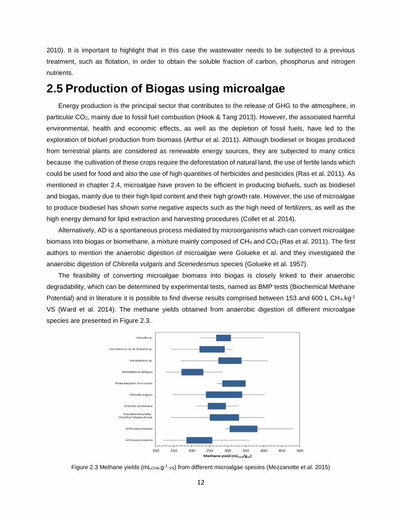
The feasibility of converting microalgae biomass into biogas is closely linked to their anaerobic
degradability, which can be determined by experimental tests, named as BMP tests (Biochemical Methane
Potential) and in literature it is possible to find diverse results comprised between 153 and 600 L CH4.kg-1
VS (Ward et al. 2014). The methane yields obtained from anaerobic digestion of different microalgae
species are presented in Figure 2.3.
Figure 2.3 Methane yields (mLCH4.g-1 VS) from different microalgae species (Mezzanotte et al. 2015)
13
An interesting characteristic of microalgae composition that favors their degradability over that of other
plants is the absence of lignin as well as the low content of hemicellulose (Chen et al. 2013).Since these
two compounds are slowly biodegradable, the anaerobic digestion of microalgae biomass is more
advantageous because it presents higher conversion rates and efficiencies when compared with other
plants (Vergara-Fernández et al. 2008).
However, one of the major constraints to take into account in this process is the presence of a cell wall
and its composition. The complex cell wall structure of some microalgae species, mainly composed of
cellulose, hemicellulose, pectin and glycoprotein, makes it highly resistant to bacterial attack, thus leading
to low yields of biomethane production (Passos et al. 2013). Therefore, to overcome this constraint it is
necessary to do a pretreatment, such as a heat treatment with temperatures between 70-100 °C, a thermo-
chemical combined treatment, the application of ultrasounds or of freeze/thaw cycles (Ward et al. 2014).
It should be added that the production of biogas is also linked to the composition of microalgae biomass,
particularly to the lipid content, since lipids have a higher theoretical methane potential than proteins and
carbohydrates (Zamalloa et al. 2011). The lipid content allows the decision between biogas production and
biodiesel production, taking into account which one is energetically more advantageous. It has been
estimated that with a lipid content of less than 40%, the anaerobic digestion is more convenient (Sialve et
al. 2009). However, the extraction of lipids for biodiesel production before AD of the residual biomass can
be beneficial for anaerobic digestion since high lipid content can be inhibitory (Sialve et al. 2009)(Park & Li
2012)
Another important factor that influences anaerobic digestion is the ratio of carbon to nitrogen present in
microalgae species (Sialve et al. 2009) and the data reported in the literature shows that this ratio (C/N)
varies from 4.16 to 7.82 for microalgae species that have already been explored for anaerobic digestion
(Ward et al. 2014). However, when the C/N ratio is lower than 20, there is an imbalance between carbon
and nitrogen requirements for the anaerobic bacterial community, thus leading to the release of nitrogen in
the form of ammonia, which can be inhibitory for the methanogenic bacteria and result in VFAs accumulation
(Sialve et al. 2009).Therefore, one solution to overcome this problem is the co-digestion of microalgae with
other waste streams or biomass with high C/N ratio, consequently leading to an optimal ratio (Santos-
Ballardo et al. 2016). Many substrates have already been tested for co-digestion in laboratory scale,
including glycerol, mixtures of oils and fats, residues from the paper industry and crop residues, such as
corn (Santos-Ballardo et al. 2016).
Finally, it is important to refer the advantage in complementing anaerobic digestion with cultivation and
production of microalgae due to the possibility of recycling nutrients. Regarding carbon, it is mainly released
as a constituent of biogas and microalgae present the ability to purify the biogas since they can recover the
CO2 (Zamalloa et al. 2011). Similarly, the hydrolytic process that takes place inside the anaerobic digesters
allows to dissolve the nutrients contained in the algae cells and these nutrients become present in the liquid
phase of the obtained digestate (Ward et al. 2014). Therefore, this digestate can be fed back and used as
a nutrient source for new algae growth, significantly reducing the need for fertilizers.
14
2.6 Microalgae cultivation
Microalgae cultivation at large scale can be done in closed systems, named as photobioreactors
(PBRs), or in open systems, such as lakes and ponds.
Photobioreactors are flexible systems which can be optimized according to the physical and biological
characteristics of the microalgae to be cultivated (Mata et al. 2010). These closed systems do not allow a
direct exchange of gases or contaminants between the microalgae culture and the atmosphere and they
are designed to optimize the diffusion of light, whether natural or artificial. Depending on their shape and
design, PBRs present various advantages over open ponds since they offer an easier control of the
parameters (pH, oxygen, temperature and nutrients), reduce CO2 losses, prevent evaporation, allow to
obtain higher microalgae densities and higher volumetric productivities and offer a safer environment, thus
minimizing the risk of contamination (Mata et al. 2010). Despite these advantages, PBRs present some
limitations, such as overheating, oxygen accumulation, bio-fouling, high building and operating costs , as
well as difficulty in scaling up (Mata et al. 2010).
Among the various photobioreactor types, tubular photobiorreactor is one of the most suitable types
for outdoor mass cultures. These photobioreactors are constructed with either glass or plastic tube and they
appear either as straight tubes arranged flat on the ground or as long vertical rows (Abdel-Raouf et al. 2012).
Tubular photobioreactors are very suitable for outdoor cultures since they have large illumination surface
area, high productivities and are relatively cheap (Mata et al. 2010). However, one of the major constraints
of this design is a poor mass transfer, which is a big problem in scaling up (Ugwu et al. 2008).
There are also flat-plate photobioreactors that are characterized by a large illumination surface area
and consist of flat panels made of transparent material. Although these photobioreactors lead to a very low
accumulation of dissolved oxygen when compared to the tubular photobioreactors, they also present some
drawbacks, including difficulty in controlling temperature and the scale up requirement for many
compartments and support material (Ugwu et al. 2008).
Over the years, the cultivation of microalgae in vertical column systems, such as air lifts and bubble
columns, has also been developed since they are able to provide a good mixing, low shear stress, high
mass transfer, high scalability potential and low energy consumption (Mata et al. 2010). The columns are
positioned vertically, made of transparent material and aerated from the bottom. Compared to other types
of photobioreactors, these vertical columns have a major disadvantage of having lower surface exposed to
light (Ugwu et al. 2008).
The other systems for microalgae cultivation, known as open ponds, include natural waters (lakes,
lagoons, ponds) and artificial ponds or containers and the most frequently used systems consist of shallow
big ponds, tanks, circular ponds and raceway ponds. When compared to closed systems, open ponds are
easier to construct and operate, they are cheaper and they are easier to clean after cultivation (Abdel-Raouf
et al. 2012). However, open ponds present major limitations such as reduced light utilization by microalgae,
evaporative losses, diffusion of CO2 to the atmosphere, extreme dependence on weather conditions,
15
requirement of large areas of land and very low mass transfer rates, thus leading to low biomass
productivities (Ugwu et al. 2008).
Finally, the cultivation of microalgae is completed with a system of microalgae collection from the
dispersed phase in which they are grown and it consists in a separation of the solid phase (microalgae) from
the liquid (the growth medium). As mentioned before, the harvesting of microalgae is a challenging phase
of microalgae biomass production due to their small size and low concentration in the growth medium (Li et
al. 2008). The choice of harvesting technique depends on the microalgae characteristics, such as size,
density, and the value of the target products (Olaizola 2003). Generally, this process involves two phases:
bulk harvesting, which consists on separating biomass from the bulk suspension by flotation, flocculation or
gravity sedimentation, and thickening, which consists in concentrating the slurry by centrifugation, filtration
and ultrasonic aggregation (Brennan & Owende 2010).
2.7 Microalgae classification and characterization
The term algae was first introduced by Linnaeus in 1753 to refer to a group of plants, which are known
since ancient civilization. It refers to a wide group of unicellular and multicellular organisms present
worldwide in different habitats, which can grow photoautotrophically, heterotrophically and mixotrophically
(Perez-Garcia et al. 2011), depending on the different environmental conditions. In freshwater bodies and
oceans, algae and cyanobacteria (photosynthetic prokaryote organisms, once considered microalgae too)
constitute the phytoplankton and the primary producers, as they are the base of the aquatic food chain.
Microalgae are unicellular eukaryotic photosynthetic organisms, with an average size between 2 and
40 µm (Brennan & Owende 2010) that convert CO₂ and radiant energy of the sun into sugars for their energy
and biosynthetic metabolism, and into oxygen. These microscopic algae typically found in freshwater or
marine systems, can exist individually or in group and do not contain stems and roots as do higher plants.
There is a vast biodiversity of microalgae and it is estimated an existence of 200 000-800 000 species but
only around 50 000 species have been studied and described (Renuka et al. 2015). Thus, this vast
biodiversity and the tendency of microalgae to adapt to extreme habitats encourages scientists to study and
to identify promising species in order to use and develop more efficient microalgae based technologies for
wastewater treatment (Roy et al., 2011).
Microalgae are categorized into diverse classes mainly considering their life cycle, pigmentation and
cellular structure (Brennan & Owende 2010). Although the classification and division of algae and
microalgae in groups is very controversial, the most known and studied algae are divided in Euglenophyta,
Cryptophyta, Dinophyta, Chlorophyta, Heterokontophyta, Rhodophyta and Haptophyta. The following
paragraphs represent a general description of the different classes, including the shape and the
environments in which they can be found ( Roy et al., 2011).
The Euglenophyta are unicellular ovoid or fusiform microalgae, with one or two flagella, mostly found in
freshwater habitats, but also in brackish and marine environments. These microalgae have a grass green
color and the common marine forms are 40-60 µm long, sometimes up to 500 µm, and around 10 µm wide.
More than 800 species have been discovered until now.
16
The Cryptophyta consists mainly of photosynthetic nanoplanktonic flagellates and their color can be
red, blue-green or gold, depending on their complement of photosynthetic pigments. These algae are
commonly found in freshwater, brackish and marine environments and around 200 photosynthetic species
have already been discovered. Regarding their shape and size, they are ovoid asymmetrical unicells, with
an average size of 6-20 µm and with two flagella.
The Dinophyta, also known as dinoflagellates, are a diverse and complex group of unicellular flagellates,
with a size comprised between 5 and 2000 µm and are constituted by two flagella. These organisms can be
found in tropical, subtropical, temperate and polar oceans, also in freshwaters and at least 2000 species
have been discovered, half of them being photosynthetic species. Dinoflagellates can easily form symbiotic
relations with other eukaryotic microalgae and they can have diverse colors.
The Chlorophyta are photosynthetic eukaryotes which belong to the green algae lineage. These
microalgae are mostly found in marine environments as planktonic individual cells and at least 17000
species have been discovered, being Chlorella, Scenedesmus and Dunaliella the most important species.
Their morphology can be presented as small green flagellates, naked, coccoid or ovoid, with 10-40 µm in
diameter.
Within Bacillariophyta group, there are diatoms, which are probably the best known of all the heterokont
unicellular planktonic algae. Diatoms are unicellular or colonial organisms (2-200 µm) with no flagella and
presenting the particularity of having a silica glass case. These organisms can be found in freshwater and
marine environments and more than 100 000 living species have been defined.
The algae division Rodophyta, also known as red algae, includes primitive eukaryotes that belong to a
very ancient lineage and it comprises a widely variety of pigmented unicells and macrophytes. Though only
a few genera of unicells are known, more than 4000 macropythes species have already been screen and
studied. The red algae are mainly found in marine environments, especially in hot and tropical waters but
they can also be found in estuaries, freshwater and soils. Regarding their form and shape, they may appear
as coccoid unicells or in colonies in a polysaccharide matrix, they don´t have flagella and their average size
is 5-15 µm.
The Haptophyta division comprises unicellular species, mostly photosynthetic flagellates, which are
mainly found in the nanoplankton of marine environments, especially in tropical waters. These microalgae
have an average size of 5-10 µm, two flagella and they can have a variety of forms including coccoid,
colonial, amoeboid and filamentous stages.
2.8 Microalgae metabolism
Generally, the organisms that exist in the world can be divided into two main categories, in autotrophic
and heterotrophic organisms. Autotrophs are organisms that are able to synthetize all the complex organic
compounds that they need, such as proteins, fats and carbohydrates, from nutrients and inorganic material,
generally using energy from light (photosynthesis) or from inorganic chemical reactions (chemosynthesis)
and CO2 as carbon source. On the other hand, heterotrophs are the organisms that cannot fix carbon and
that use organic compounds for growth.
17
As mentioned before, microalgae are considered as autotroph organisms and are the base of the
aquatic food chain, since they can produce organic matter through photosynthesis. Photosynthesis is a
fundamental process for the existence of life on Earth and it can be defined as a redox reaction, in which
inorganic carbon and water are converted into oxygen and organic compounds, in the presence of light
energy. Carbon is a constituent of all the organic compounds and is the main microalgae biomass element,
contributing between 17% and 65% of dry weigh depending on the species (Markou et al. 2014). However,
most of the species contain 50% of carbon (Richmond 2004).
Carbon is mostly taken up by photosynthetic organisms in the form of CO2, however since microalgae
live in aquatic environments, when CO2 is dissolved in water, it reacts with water molecules, creating a weak
acid buffer system, and in this system the form and the availability of inorganic dissolved carbon depends
on diverse parameters, such as pH and temperature (Markou et al. 2014). Consequently, microalgae
developed mechanisms that allow the uptake of different dissolved inorganic carbon, like HC03−, for
photosynthesis (Markou et al. 2014).
All the photosynthetic organisms comprise organic pigments to absorb the light energy, each one
capable of absorbing light at different wavelengths. The most important pigment is chlorophyll which
contains a heterocyclic ring (porphyrin ring). This ring has a magnesium atom at the center and is bonded
to a hydrocarbon chain that makes the chlorophyll insoluble in water (Borowitzka et al. 2016). The main
chlorophylls are chlorophyll a, absorbing mainly the blue-violet and red light, and chlorophyll b, which mainly
absorbs blue and orange light (Borowitzka et al., 2016). Other two major organic pigments are carotenoids
and phycobilins, which absorb light in the wavelength of blue-green and violet (Borowitzka et al., 2016).
Photosynthesis is divided in two stages, the light dependent reactions and the independent reactions
(Chisti et al., 2014). The first process consists in a light-dependent series reaction that occurs in the grana
and which requires the direct light energy in order to produce energy-carrier molecules that are further used
in the second phase. So, in this phase the light is captured by chlorophyll to produce ATP and at the same
time water is split, releasing oxygen, free electrons and hydrogen ions. Then, the free electrons react with
NADP+ and convert it in NADPH. In the second process, also called as dark reactions, ATP and NADPH
molecules are used to convert CO2 into carbohydrates (carbon fixation) through a reduction process that
occurs in the stroma of chloroplasts.
The fixation of carbon dioxide occurs in the stroma of chloroplasts and it can be achieved through Calvin
Cycle, also known as C3 cycle, which is the most important process for carbon fixation that occurs in
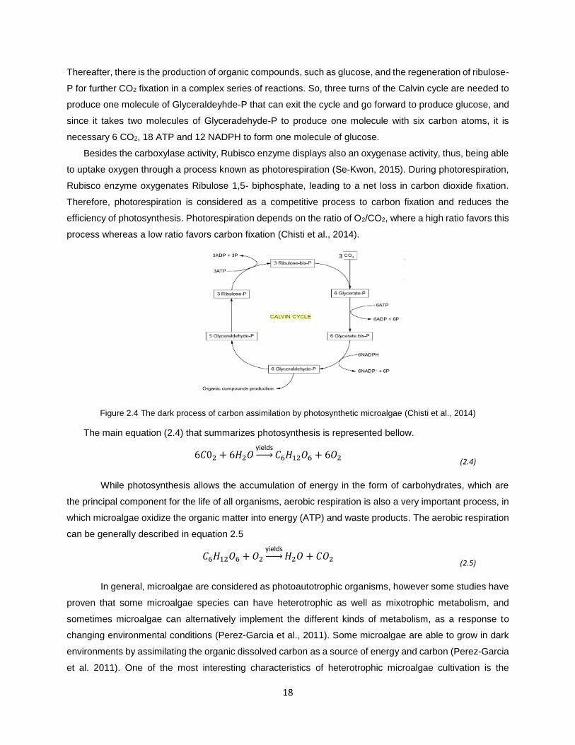
microalgae (Chisti et al., 2014). As described in Figure 2.4, the Calvin cycle is divided in four main steps
and there is only one enzyme responsible for CO2 fixation, ribulose 1,5-biphosphate
carboxylase/oxygenase, also named as Rubisco. In the first phase, which is named as Carboxylation, CO2
is incorporated in the five-carbon sugar ribulose bisphosphate (Ribulose-bis-P) to produce two molecules
of phosphoglycerate (Glycerate-P) and this reaction is catalyzed by the enzyme Rubisco. Then, in the
second step there is the reduction of Glycerate-P into 3-carbon sugars (Triose-P) by two sub steps, which
are the phosphorylation of Glycerate-P to produce diphosphoglycerate (Glycerate-bis-P) in the presence of
ATP and, the reduction of Glycerate-bis-P to phosphoglyceraldehyde (Glyceraldehyde-P) by NADPH.
18
Thereafter, there is the production of organic compounds, such as glucose, and the regeneration of ribulose-
P for further CO2 fixation in a complex series of reactions. So, three turns of the Calvin cycle are needed to
produce one molecule of Glyceraldeyhde-P that can exit the cycle and go forward to produce glucose, and
since it takes two molecules of Glyceradehyde-P to produce one molecule with six carbon atoms, it is
necessary 6 CO2, 18 ATP and 12 NADPH to form one molecule of glucose.
Besides the carboxylase activity, Rubisco enzyme displays also an oxygenase activity, thus, being able
to uptake oxygen through a process known as photorespiration (Se-Kwon, 2015). During photorespiration,
Rubisco enzyme oxygenates Ribulose 1,5- biphosphate, leading to a net loss in carbon dioxide fixation.
Therefore, photorespiration is considered as a competitive process to carbon fixation and reduces the
efficiency of photosynthesis. Photorespiration depends on the ratio of O2/CO2, where a high ratio favors this
process whereas a low ratio favors carbon fixation (Chisti et al., 2014).
Figure 2.4 The dark process of carbon assimilation by photosynthetic microalgae (Chisti et al., 2014)
The main equation (2.4) that summarizes photosynthesis is represented bellow.
6𝐶02 + 6𝐻2𝑂yields→ 𝐶6𝐻12𝑂6 + 6𝑂2
(2.4)
While photosynthesis allows the accumulation of energy in the form of carbohydrates, which are
the principal component for the life of all organisms, aerobic respiration is also a very important process, in
which microalgae oxidize the organic matter into energy (ATP) and waste products. The aerobic respiration
can be generally described in equation 2.5
𝐶6𝐻12𝑂6 +𝑂2yields→ 𝐻2𝑂 + 𝐶𝑂2
(2.5)
In general, microalgae are considered as photoautotrophic organisms, however some studies have
proven that some microalgae species can have heterotrophic as well as mixotrophic metabolism, and
sometimes microalgae can alternatively implement the different kinds of metabolism, as a response to
changing environmental conditions (Perez-Garcia et al., 2011). Some microalgae are able to grow in dark
environments by assimilating the organic dissolved carbon as a source of energy and carbon (Perez-Garcia
et al. 2011). One of the most interesting characteristics of heterotrophic microalgae cultivation is the
19
elimination of light requirements, allowing the use of innovative bioreactors without light constraints in their
design (Bumbak et al., 2011). However, only few species have proven to grow under heterotrophic
conditions (Lowrey et al., 2015) and this type of cultivation presents some disadvantages such as an
addition of potential costs due to the need of meeting the organic carbon requirement which is most
commonly delivered from glucose (Lowrey et al., 2015); diminishing of the pigmentation and of the
production of high value phytochemicals of the microalgae cells due to dark reactions, thus causing
economic problems in the cultivation (Mata et al., 2010) and production of carbon dioxide from the
respiration of organic carbon during growth (Perez-Garcia et al., 2011).
Regarding mixotrophic conditions, it is defined as a mix of autotrophic and heterotrophic conditions,
which means that microalgae are able to perform photosynthesis and consume CO2 and organic matter as
a carbon source (Lowrey et al., 2015). For example, (Heredia-Arroyo et al. 2011) reported that Chlorella
vulgaris was able to grow under autotrophic, heterotrophic and mixotrophic conditions and that the
mixotrophic conditions could produce more biomass concentration than the other conditions. However,
mixotrophic microalgae, overall, are poorly studied and the available examples are quite limited to a few
species. Hence, there should be more studies on mixotrophic microalgae since it takes advantage of both
organic and inorganic resources to obtain maximum biomass production and, particularly interesting when
integrating microalgae cultivation with wastewater treatment where wastewater is usually turbid and the sun
light cannot penetrate well into the core of the wastewater body (Heredia-Arroyo et al. 2011).
However, certain species are characterized as obligate photoautotrophs and some species are able
of having a photoautotrophic and heterotrophic metabolism simultaneously or sequentially (Perez-Garcia et
al., 2011). The universal reason why some microalgae are obligate photoautotrophs is still unknown,
however one of the proposed theories claims that it is a result of a deficiency in the cellular consumption of
vital substrates, mainly sugars (Chen & Chen, 2006). For example Phaeodactylum tricornutum is a
phototrophic microalga that became able to grow after the insertion of a gene which encodes a transporter
for glucose (Morales-Sanchez et al., 2014).
Besides light and CO2, microalgae need micronutrients and macronutrients for their growth. The
micronutrients necessary for the growth of microalgae include potassium, metals, sulfur and calcium, while
regarding macronutrients, microalgae need nitrogen and phosphorus compounds (Cao & Orrù, 2014).
Nitrogen is a fundamental compound since it allows the production of amino acids and nucleic acids. In the
case of phosphorus, it can be incorporated in a large variety of organic compounds, such as sugars
phosphates, phospholipids and nucleotides.
2.9 Parameters that influence microalgae growth
As described in Figure 2.5, the growth cycle of microalgae in batch consists of 5 phases (Cao & Orrù,
2014):
1. Lag phase or Induction phase, during which microalgae adapt to the environment and to the
new conditions thus, there is no growing of culture density;
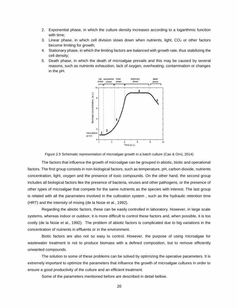
20
2. Exponential phase, in which the culture density increases according to a logarithmic function
with time;
3. Linear phase, in which cell division slows down when nutrients, light, CO2 or other factors
become limiting for growth;
4. Stationary phase, in which the limiting factors are balanced with growth rate, thus stabilizing the
cell density;
5. Death phase, in which the death of microalgae prevails and this may be caused by several
reasons, such as nutrients exhaustion, lack of oxygen, overheating, contamination or changes
in the pH.
Figure 2.5 Schematic representation of microalgae growth in a batch culture (Cao & Orrù, 2014)
The factors that influence the growth of microalgae can be grouped in abiotic, biotic and operational
factors. The first group consists in non-biological factors, such as temperature, pH, carbon dioxide, nutrients
concentration, light, oxygen and the presence of toxic compounds. On the other hand, the second group
includes all biological factors like the presence of bacteria, viruses and other pathogens, or the presence of
other types of microalgae that compete for the same nutrients as the species with interest. The last group
is related with all the parameters involved in the cultivation system , such as the hydraulic retention time
(HRT) and the intensity of mixing (de la Noüe et al., 1992).
Regarding the abiotic factors, these can be easily controlled in laboratory. However, in large scale
systems, whereas indoor or outdoor, it is more difficult to control these factors and, when possible, it is too
costly (de la Noüe et al., 1992). The problem of abiotic factors is complicated due to big variations in the
concentration of nutrients in effluents or in the environment.
Biotic factors are also not so easy to control. However, the purpose of using microalgae for
wastewater treatment is not to produce biomass with a defined composition, but to remove efficiently
unwanted compounds.
The solution to some of these problems can be solved by optimizing the operative parameters. It is
extremely important to optimize the parameters that influence the growth of microalgae cultures in order to
ensure a good productivity of the culture and an efficient treatment.
Some of the parameters mentioned before are described in detail bellow.
21
2.9.1 Nutrients Among all factors that influence microalgae growth, nutrients availability is one of the most important
factors to take into account during microalgae cultivation. Nutrient availability is crucial for cell division and
for intracellular metabolic activities and once nutrients become limited, a steady decline takes place in
microalgae growth cycle (Cao & Orrù, 2014).
As mentioned before, for their growth microalgae need micronutrients (Mg, Zn, Fe, K, Na, etc.) and
macronutrients (C, P, N) as well as dissolved CO2, transferred from the gas phase (Cao & Orrù 2014).
Besides CO2, whose importance has already been mentioned in the chapter 2.8, phosphorus and nitrogen
nutrients are also fundamental keys for the growth of microalgae.
2.9.1.1 Carbon
As mentioned in chapter 2.8, carbon is the main microalgae biomass element and is mostly taken
up by microalgae in the form of CO2 (Markou et al., 2014). In natural conditions, microalgae uptake CO2
from the ambient air, which contains around 360 ppmv of CO2, however, most microalgae species have
proven to tolerate and to uptake much higher concentrations, up to 150 000 ppmv (Brennan & Owende,
2010). CO2 can be supplied from three different sources, such as atmosphere, exhaust gas from power
plants and industries and soluble carbonates, like Na2CO3 and NaHCO3 (Wang et al., 2008). The use of
CO2 from the atmosphere and from exhaust gas involves an environmental advantage since it contributes
to the reduction of GHG emissions. However, the potential yield from the atmosphere is limited due to the
low concentration of CO2 (Brennan & Owende, 2010). On the other hand, CO2 capture from power plant
flue gas achieves better recovery as it contains higher concentrations, usually between 15-20% (Salih,
2011). This exhaust gas contains nitrogen oxides (NOx), sulfur oxides (SOx) and particulates (dust) causing
some constraints related to their inhibitory effects on microalgae growth (Lara-Gil et al., 2014). However,
some studies have proven that some microalgae species can tolerate NOx and SOx to some levels and use
it as a source of nutrients (Chiu et al., 2011). For example, in an aqueous system NOx partially dissolves
and oxidizes into nitrite, which could be used as nutrient for microalgae. Regarding sulfur dioxide, it can
generate bisulfite, which can severely affect the pH of the culture or can generate sulfate that can be
assimilated by microalgae (Lara-Gil et al., 2016). Finally, it is important to refer that these gases need to be
cooled prior to the injection in the cultivation medium.
2.9.1.2 Nitrogen
After carbon, and not considering hydrogen and oxygen, nitrogen is quantitatively the most
significant element, representing approximately 1 to 10 % of the dry matter of algae cells (Richmond 2004),
and is a component of essential biochemical compounds, such as amino acids, nucleic acids and pigments
like chlorophyll. It can be taken by microalgae in its inorganic form (nitrate, ammonium ion and nitrite) and
converted in its organic form through assimilation but also, it can be taken in organic forms such as urea or
amino acids (Flynn & Butler, 1986;Perez-Garcia et al., 2011).
Ammonium is the most favorite nitrogen source for microalgae since its uptake and assimilation
process is simpler and requires less energy consumption than for other nitrogen sources (Markou et al.,
22
2014). Ammonium is transported through the membranes by a group of proteins that belong to the
ammonium transporter family (AMT) (Perez-Garcia et al., 2011). The most important path for ammonium
assimilation involves glutamine synthetase, which produces glutamine amino acid by the reaction between
ammonium and glutamate and glutamate synthase, which produces two molecules of glutamate from
glutamine and one molecule of α-ketoglutarate (De-Bashan et al., 2008).
One of the major constraints in using ammonium as a source of nitrogen is its toxicity at high
concentrations which can be due to ammonium ion or free ammonia (Markou et al., 2014). Free ammonia
is considered to be the most toxic form since it is uncharged and lipid soluble and can easily diffuse trough
the membrane into the cells, which have low control on intracellular concentration, thus becoming toxic and
damaging the photosynthetic system (Collos & Harrison, 2014). According to (Azov & Goldman, 1982) free
ammonia presents a toxic effect for very low concentrations 2 mM. The relative concentration of ionized
ammonia and free ammonia depends mainly on pH and temperature (Tosta & Mendonça, 2009).
Ammonia toxicity is a major concern to take into account when using wastewaters with high
concentrations of nitrogen, as is the case of piggery wastewaters. One of the strategies to decrease toxicity
effects is to control the pH of the medium, thus limiting the concentration free ammonia (Markou et al., 2014)
and another strategy is to dilute the wastewater to avoid the inhibitory effect of ammonia (Olguín et al.,
2003).
In addition, another important constraint to consider when using ammonium as a source of nutrient,
is that it can be lost from cultivation medium though volatilization, mainly with high pH (Markou et al., 2014).
Regarding nitrate, it is one of the major sources of inorganic nitrogen to microalgae and its
assimilation involves two reduction steps. First, nitrate is transported into the cell and a cytosolic nitrate
reductase transforms it into nitrite, then it is transported to chloroplast, where nitrite reductase converts it
into ammonium (Sanz-Luque et al., 2015). Finally, it can go through the glutamine synthetase pathway to
produce glutamine amino acid. Although usually nitrate does not present toxic effects to microalgae, at high
concentrations it can affect the microalgae growth since with the increase of nitrate, there is an increase of
nitrate reductase activity, therefore resulting in an intracellular accumulation of nitrite and ammonium, which
are toxic to the cells (Chen et al., 2009) .
Nitrite is regularly found in natural environments as an intermediate from nitrate reduction or from
ammonia oxidation, however it can also be found intracellular as a result of nitrate reduction, which was
previously described. Microalgae are able to up take nitrite from the medium, mainly through active
transportation (Markou et al., 2014), but diffusion has been also reported for green microalgae. Nitrite is
transported to chloroplast, where nitrite reductase converts it into ammonium. Then, as previously
described, it can go through the glutamine synthetase pathway to produce glutamine amino acid. Although
microalgae are able to uptake nitrite and use it as nitrogen source, at high concentrations it is a toxic
compound and presents negative impacts in microalgae growth (Chen et al., 2012). Furthermore, the uptake
of nitrite seems to be influenced by CO2 concentration since under low CO2 concentration the uptake of
nitrite is reduced, while high CO2 concentration affects positively the nitrite reductase activity, enhancing
the nitrite assimilation (Markou et al., 2014).
23
Moreover, urea and some amino acids are taken up actively and are metabolized in the cells (Pérez
Garcia, et al., 2011). Some green microalgae seem not only to be able to use organic nitrogen, but, when
they use these molecules, their growth rate are similar or higher than when they use other inorganic forms
of nitrogen. However, the possibility to use organic nitrogen compounds as nitrogen resource depends on
the species.
It has to be highlighted that when different nitrogen sources are simultaneously present in the
medium, microalgae firstly uptake the one with more affinity depleting it, and then they uptake the others.
2.9.1.3 Phosphorus
Phosphorus is another macronutrient that plays an important role in the metabolic processes of
microalgae, forming many functional and structured compounds required for the growth and development
of microalgae. Phosphorus is present in different organic molecules, such as nucleic acids, membrane
phospholipids and ATP (Geider & Roche 2011) and its biomass content varies between 0.05% and 3.3%
(Richmond, 2004)
Phosphorus is assimilated by microalgae mainly as orthophosphate, but other inorganic and organic
forms can also be used for microalgae growth (Markou et al., 2014). Regarding dissolved organic
phosphorus (DOP), it can either be actively up taken into the cells or it can suffer extracellular mineralization
by phosphatase enzymes (Dyhrman & Ruttenberg, 2006). However, the uptake of DOP depends on its
chemical composition. In fact, most of the DOP compounds cannot be directly assimilated by microalgae
and therefore, these compounds need to be mineralized (Dyhrman & Ruttenberg, 2006). In the case of
inorganic phosphorus forms other than orthophosphates, it is necessary to convert them into
orthophosphates in order to have an efficient uptake by microalgae and this is also mediated by
phosphatase enzymes (Markou et al., 2014). These enzymes can be intracellular, extracellular or attached
to the cell wall of microalgae.
The uptake of phosphorus is affected by the cell condition and by environmental factors, such as
pH, temperature, light and the concentration of the ions Na+, Mg2+ and K+ (Markou et al., 2014). The cellular
production of phosphatase enzymes is increased when phosphorus availability decreases and when
microalgae become phosphorus limited or starved (Dyhrman & Ruttenberg, 2006).
Another interesting fact is that under sufficient phosphorus supply, microalgae are able to
accumulate intracellular phosphorus reserves as polyphosphate granules and this reserves can be used as
phosphorus source when phosphate in the culture medium is depleted. This process is named as luxury
uptake (Brown & Shilton, 2014).
Finally, another parameter to be controlled is the Redfield ratio, which is the atomic ratio between
carbon, nitrogen and phosphorus found in phytoplankton. A stoichiometric formula for the most common
elements in algae cells is defined as C106H181O45N16P (Choi & Lee, 2015), thus the optimal Redfield ratio for
algae cultivation is assumed to be 106:16:1 and this parameter allows to determine which nutrient is limiting
(Geider & Roche, 2011). However, N:P ratio has an extra interest and it has shown to affect the growth,
cellular elements and biochemical composition of the algae (Rasdi & Qin, 2014). According to (Choi & Lee,
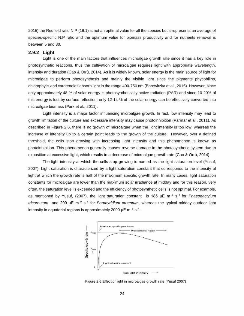
24
2015) the Redfield ratio N:P (16:1) is not an optimal value for all the species but it represents an average of
species-specific N:P ratio and the optimum value for biomass productivity and for nutrients removal is
between 5 and 30.
2.9.2 Light Light is one of the main factors that influences microalgae growth rate since it has a key role in
photosynthetic reactions, thus the cultivation of microalgae requires light with appropriate wavelength,
intensity and duration (Cao & Orrù, 2014). As it is widely known, solar energy is the main source of light for
microalgae to perform photosynthesis and mainly the visible light since the pigments phycobilins,
chlorophylls and carotenoids absorb light in the range 400-750 nm (Borowitzka et al., 2016). However, since
only approximately 48 % of solar energy is photosynthetically active radiation (PAR) and since 10-20% of
this energy is lost by surface reflection, only 12-14 % of the solar energy can be effectively converted into
microalgae biomass (Park et al., 2011).
Light intensity is a major factor influencing microalgae growth. In fact, low intensity may lead to
growth limitation of the culture and excessive intensity may cause photoinhibition (Parmar et al., 2011). As
described in Figure 2.6, there is no growth of microalgae when the light intensity is too low, whereas the
increase of intensity up to a certain point leads to the growth of the culture. However, over a defined
threshold, the cells stop growing with increasing light intensity and this phenomenon is known as
photoinhibition. This phenomenon generally causes reverse damage in the photosynthetic system due to
exposition at excessive light, which results in a decrease of microalgae growth rate (Cao & Orrù, 2014).
The light intensity at which the cells stop growing is named as the light saturation level (Yusuf,
2007). Light saturation is characterized by a light saturation constant that corresponds to the intensity of
light at which the growth rate is half of the maximum specific growth rate. In many cases, light saturation
constants for microalgae are lower than the maximum solar irradiance at midday and for this reason, very
often, the saturation level is exceeded and the efficiency of photosynthetic cells is not optimal. For example,
as mentioned by Yusuf, (2007), the light saturation constant is 185 μE m−2 s−1 for Phaeodactylum
tricornutum and 200 μE m−2 s−1 for Porphyridium cruentum, whereas the typical midday outdoor light
intensity in equatorial regions is approximately 2000 μE m−2 s−1 .
Figure 2.6 Effect of light in microalgae growth rate (Yusuf 2007)
25
Since the fluctuation of light intensities in the outdoor cultures can affect microalgae growth due to
reduced light intensity during the rainy days or to excessive light intensity during summer days, the
cultivation of microalgae with artificial light (LED or fluorescent lamps) is a good solution when the operation
costs are justified (Zhao et al., 2013).
Finally, the duration of light is also an important factor to take into account during microalgae growth
(Al-Qasmi et al., 2012). Microalgae need a light/dark system for an efficient photosynthesis since they need
light for a photochemical phase to produce ATP and NADPH, and they need a dark phase to produce the
crucial compounds for their growth. For this reason, if the light is artificial it is necessary to maintain a
light/dark (LD) cycle similar to the natural conditions (maximum 16:8 LD and usually, 14:10 LD or 12:12)
(Mezzanotte et al. 2015).
2.9.3 pH The monitoring of a medium´s pH during algae growth is an important tool to analyze the
performance of the photosynthetic processes, since during photosynthesis microalgae uptake dissolved
CO2 from the medium and consequently, the pH increases. Although pH variation can be an indicator of the
photosynthesis performance, it can also affect the kinetics of microalgae growth as it can modify the
distribution of carbon dioxide species and carbon availability, it can change the availability of nutrients and
trace metals, and at extreme pH levels it can cause direct physiological effects (Cao & Orrù, 2014)
The pH is closely connected to the concentrations of HC03−, CO2 and C03
2− of the carbonate system
because as pH increases, carbonate concentration increases and the concentrations of carbon dioxide and
bicarbonate decrease. The concentration of carbon dioxide in the medium is influenced by photosynthesis,
respiration, water temperature and oxidative decomposition of organic matter (Zang et al., 2011). During
the photosynthetic process, microalgae quickly uptake carbon dioxide, which causes a shift of the
equilibrium, favoring the decomposition of HC03− and thus, leading to a pH increase and a decrease of the
partial pressure of CO2 when the replacement process of CO2 is slower that the utilization. The replacement
of CO2 includes the respiration, the fermentation, the influx of atmospheric CO2 and dehydration and
hydration reactions of dissolved CO₂ (Chen & Durbin, 1994). Therefore, the production of CO2 by aquatic
respiration processes may inhibit the decomposition HC03− and consequently, result in the decrease of pH.
Many studies on the effect of pH in microalgae cultures have defined the optimum pH value as the
parameter corresponding to the highest growth rate of microalgae, differing from species to species. As an
example, regarding two of the most important species, the optimal pH is 6.5 for Chlorella vulgaris and 7 for
Scenedesmus obliquus (Hodaifa et al., 2009). Generally, microalgae present a neutral or slightly alkaline
optimum pH (7-9), though some species are able to grow in acidic conditions and this may be due to the
fact that the photosynthetic system is inside chloroplasts, which are surrounded by cytoplasm. Since
cytoplasm presents a neutral pH, when microalgae are subject to acidic environments, chloroplasts can be
protected, subsequently protecting chlorophyll and the photosynthetic system (May, 1997).
As mentioned before, pH is the main parameter that influences the relative concentrations of ionized
ammonia and free ammonia. Another important point is that the assimilation of different nitrogen sources
26
influences the pH of the culture medium since when ammonium is assimilated, pH may decrease due to the
release of H+ ions and when nitrate is assimilated there is the release of OH- (Markou et al., 2014).
2.9.4 Temperature Temperature is one of the main factors that affects microalgae growth since it influences the nutrient
requirements, the nature of metabolism, the biomass concentration and the metabolic reaction rates of
microalgae. Normally, at low temperatures microalgae growth rates decrease, whereas at high
temperatures their metabolic rates accelerate (Muñoz & Guieysse, 2006).
In general, each microalgae species is characterized by having an optimum growth temperature,
at which enzymes present the highest activity, thus providing a maximum growth rate and for most of the
strains, this temperature ranges between 25 and 28°C (Richmond, 2004). Bellow optimal temperatures, a
temperature increase causes an enhancement of enzymatic activities that are connected with the Calvin
Cycle, thus leading to a more efficient photosynthesis and cell division (Ras et al. 2013). On the other hand,
above the optimal temperature, microalgae growth rate tends to decrease, mainly due to heat stress, which
can denature essential proteins/enzymes that are involved in the photosynthetic process (Ras et al., 2013).
Finally, if the temperature of the culture is not adequate to obtain the desired microalgae production,
it is possible to control and regulate the temperature with an immersion heat system or exploiting the heat
of the exhaust gas used to provide CO2 to the system.
2.9.5 Dissolved Oxygen Concentration As it is well known, oxygen is a product of photosynthesis. However, high concentrations of
dissolved oxygen can limit microalgae growth. The main two mechanisms that negatively influence
microalgae growth are the competitive effect of O2 on Rubisco (photorespiration) and the photo-inhibition,
which in the presence of high oxygen concentrations and high irradiance level causes cell damage of
photosystem II with the production of reactive oxygen species (ROS) (Raso et al., 2011). Generally, with
the aim of preventing inhibition and damage, the maximum tolerable dissolved oxygen level should not
exceed around 400% of air saturation (Chisti, 2007).
Fortunately, high levels of dissolved O2 are not a big problem in biodegradation processes, such as
wastewater treatment, due to the continuous consumption of O2 by bacteria (Muñoz & Guieysse, 2006).
2.9.6 Presence of other microorganisms As mentioned before, the biotic factors also have an impact in microalgae growth since they are linked
to the presence of other living organisms. So, these factors include the presence of pathogens (fungus,
bacteria, virus), the competition between different microalgae species, since some microalgae have lower
productivities than others, and the presence of predators, such as rotifers.
The presence of organisms which alter the normal functional characteristics of microalgae cultivation
can be minimized by abruptly changing some parameters of the culture, such as pH, temperature and light
radiation (Mata et al., 2010).
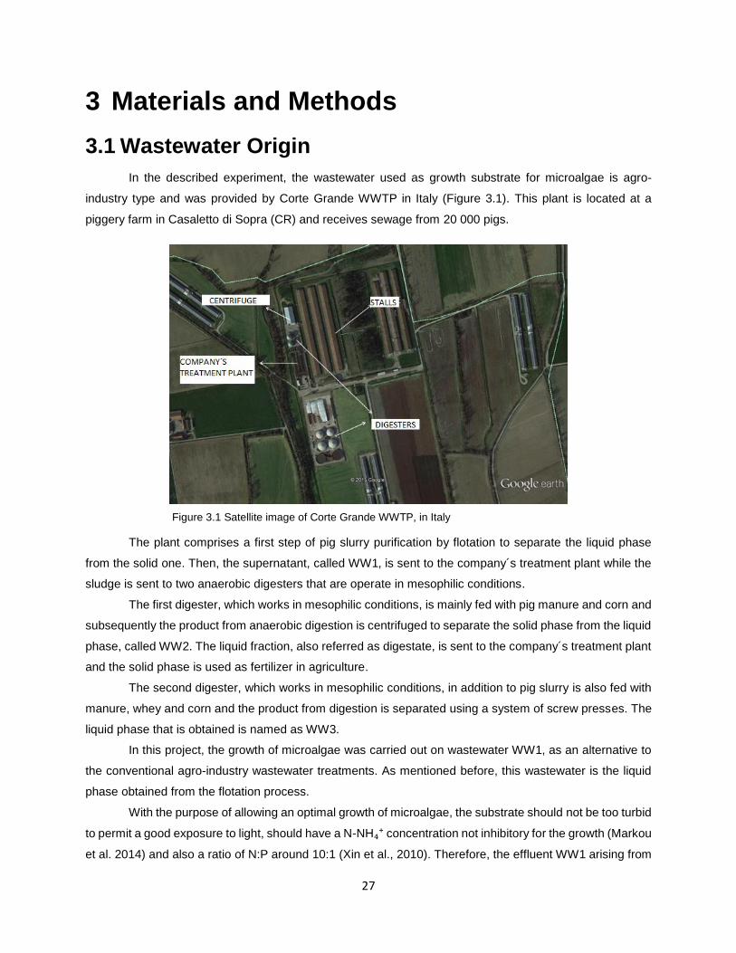
27
3 Materials and Methods
3.1 Wastewater Origin
In the described experiment, the wastewater used as growth substrate for microalgae is agro-
industry type and was provided by Corte Grande WWTP in Italy (Figure 3.1). This plant is located at a
piggery farm in Casaletto di Sopra (CR) and receives sewage from 20 000 pigs.
Figure 3.1 Satellite image of Corte Grande WWTP, in Italy
The plant comprises a first step of pig slurry purification by flotation to separate the liquid phase
from the solid one. Then, the supernatant, called WW1, is sent to the company´s treatment plant while the
sludge is sent to two anaerobic digesters that are operate in mesophilic conditions.
The first digester, which works in mesophilic conditions, is mainly fed with pig manure and corn and
subsequently the product from anaerobic digestion is centrifuged to separate the solid phase from the liquid
phase, called WW2. The liquid fraction, also referred as digestate, is sent to the company´s treatment plant
and the solid phase is used as fertilizer in agriculture.
The second digester, which works in mesophilic conditions, in addition to pig slurry is also fed with
manure, whey and corn and the product from digestion is separated using a system of screw presses. The
liquid phase that is obtained is named as WW3.
In this project, the growth of microalgae was carried out on wastewater WW1, as an alternative to
the conventional agro-industry wastewater treatments. As mentioned before, this wastewater is the liquid
phase obtained from the flotation process.
With the purpose of allowing an optimal growth of microalgae, the substrate should not be too turbid
to permit a good exposure to light, should have a N-NH₄⁺ concentration not inhibitory for the growth (Markou
et al. 2014) and also a ratio of N:P around 10:1 (Xin et al., 2010). Therefore, the effluent WW1 arising from
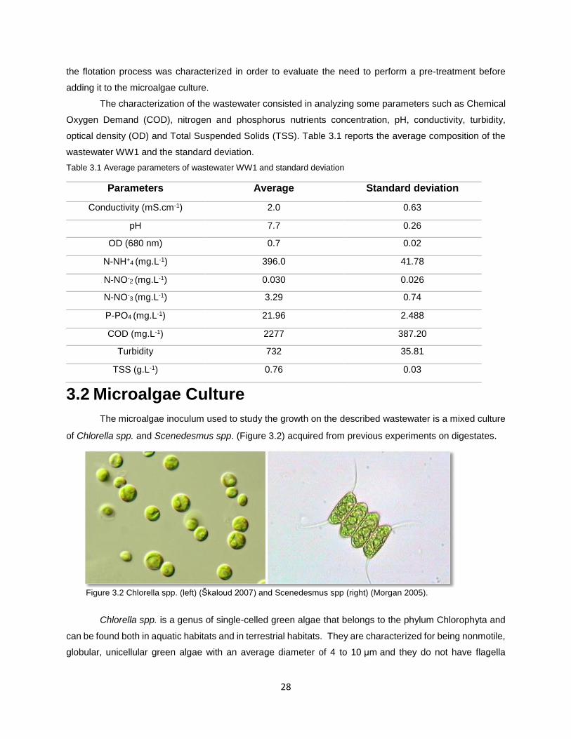
28
the flotation process was characterized in order to evaluate the need to perform a pre-treatment before
adding it to the microalgae culture.
The characterization of the wastewater consisted in analyzing some parameters such as Chemical
Oxygen Demand (COD), nitrogen and phosphorus nutrients concentration, pH, conductivity, turbidity,
optical density (OD) and Total Suspended Solids (TSS). Table 3.1 reports the average composition of the
wastewater WW1 and the standard deviation.
Table 3.1 Average parameters of wastewater WW1 and standard deviation
Parameters Average Standard deviation
Conductivity (mS.cm-1) 2.0 0.63
pH 7.7 0.26
OD (680 nm) 0.7 0.02
N-NH+4 (mg.L-1) 396.0 41.78
N-NO-2 (mg.L-1) 0.030 0.026
N-NO-3 (mg.L-1) 3.29 0.74
P-PO4 (mg.L-1) 21.96 2.488
COD (mg.L-1) 2277 387.20
Turbidity 732 35.81
TSS (g.L-1) 0.76 0.03
3.2 Microalgae Culture
The microalgae inoculum used to study the growth on the described wastewater is a mixed culture
of Chlorella spp. and Scenedesmus spp. (Figure 3.2) acquired from previous experiments on digestates.
Chlorella spp. is a genus of single-celled green algae that belongs to the phylum Chlorophyta and
can be found both in aquatic habitats and in terrestrial habitats. They are characterized for being nonmotile,
globular, unicellular green algae with an average diameter of 4 to 10 μm and they do not have flagella
Figure 3.2 Chlorella spp. (left) (Škaloud 2007) and Scenedesmus spp (right) (Morgan 2005).
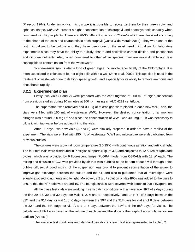
29
(Prescott 1964). Under an optical microscope it is possible to recognize them by their green color and
spherical shape. Chlorella present a higher concentration of chlorophyll and photosynthetic capacity when
compared with higher plants. There are 20-30 different species of Chlorella which are classified according
to the shape of the cells and characteristic of chlorophyll (Costa & de Morais 2014). They were one of the
first microalgae to be culture and they have been one of the most used microalgae for laboratory
experiments since they have the ability to quickly absorb and assimilate carbon dioxide and phosphorus
and nitrogen nutrients. Also, when compared to other algae species, they are more durable and less
susceptible to contamination from the wastewater.
Scenedesmus spp. is also a kind of green algae, no motile, specifically of the Chlorophyta. It is
often associated in colonies of four or eight cells within a wall (John et al. 2002). This species is used in the
treatment of wastewater due to its high-speed growth, and especially for its ability to remove ammonia and
phosphorus rapidly.
3.2.1 Experimental plan Firstly, two vials (1 and 2) were prepared with the centrifugation of 300 mL of algae suspension
from previous studies during 10 minutes at 300 rpm, using an ALC 4222 centrifuge.
The supernatant was removed and 0.12 g of microalgae were placed in each new vial. Then, the
vials were filled with 150 mL of wastewater WW1. However, the desired concentration of ammonium
nitrogen was around 200 mg.L-1 and since the concentration of WW1 was 400 mg.L-1, it was necessary to
dilute it with tap water before adding it into the vials.
After 11 days, two new vials (A and B) were similarly prepared in order to have a replica of the
experiment. The vials were filled with 150 mL of wastewater WW1 and microalgae were also obtained from
previous studies.
The cultures were grown at room temperature (20-25°C) with continuous aeration and artificial light.
The four test vials were distributed in Plexiglas supports (Figure 3.3) and subjected to 12 h/12h of light /dark
cycles, which was provided by 6 fluorescent lamps (FLORA model from OSRAM) with 18 W each. The
mixing and diffusion of CO2 was provided by air that was bubbled at the bottom of each vial through a fine
bubble diffuser. A good mixing of the suspension was crucial to prevent sedimentation of the algae, to
improve gas exchange between the culture and the air, and also to guarantee that all microalgae were
equally exposed to nutrients and to light. Moreover, a 2 g.L-1 solution of Na2HPO4 was added to the vials to
ensure that the N/P ratio was around 10. The four glass vials were covered with cotton to avoid evaporation.
All the glass test vials were working in semi batch conditions with an average HRT of 9 days during
the first 29, 35, 30 and 30 days, for vials 1, 2, A and B, respectively, and an HRT of 5 days between the
32nd and the 91st day for vial 1; of 6 days between the 39th and the 91st days for vial 2; of 6 days between
the 32nd and the 88th days for vial A and of 7 days between the 32nd and the 88th days for vial B. The
calculation of HRT was based on the volume of each vial and the slope of the graph of accumulative volume
addition (Annex I).
The average test conditions and standard deviations of each vial are represented in Table 3.2.
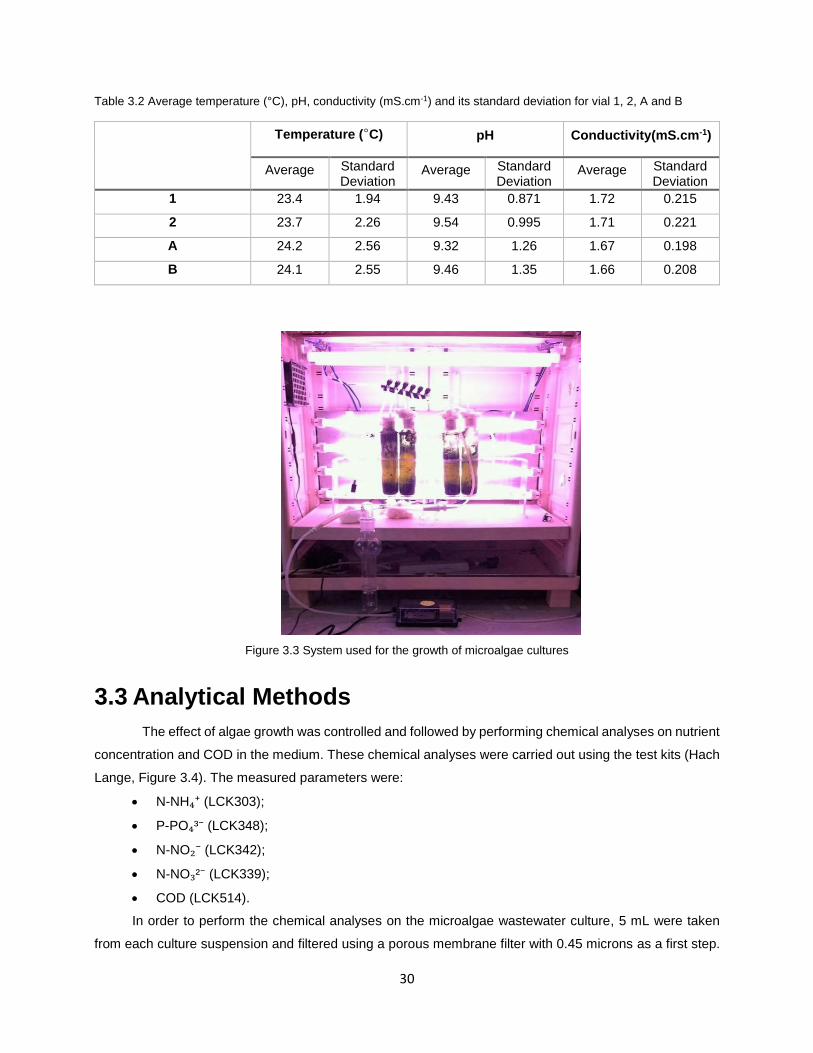
30
Table 3.2 Average temperature (°C), pH, conductivity (mS.cm-1) and its standard deviation for vial 1, 2, A and B
Temperature (°C) pH Conductivity(mS.cm-1)
Average Standard Deviation
Average Standard Deviation
Average Standard Deviation
1 23.4 1.94 9.43 0.871 1.72 0.215
2 23.7 2.26 9.54 0.995 1.71 0.221
A 24.2 2.56 9.32 1.26 1.67 0.198
B 24.1 2.55 9.46 1.35 1.66 0.208
Figure 3.3 System used for the growth of microalgae cultures
3.3 Analytical Methods
The effect of algae growth was controlled and followed by performing chemical analyses on nutrient
concentration and COD in the medium. These chemical analyses were carried out using the test kits (Hach
Lange, Figure 3.4). The measured parameters were:
N-NH₄⁺ (LCK303);
P-PO₄³⁻ (LCK348);
N-NO₂⁻ (LCK342);
N-NO₃²⁻ (LCK339);
COD (LCK514).
In order to perform the chemical analyses on the microalgae wastewater culture, 5 mL were taken
from each culture suspension and filtered using a porous membrane filter with 0.45 microns as a first step.
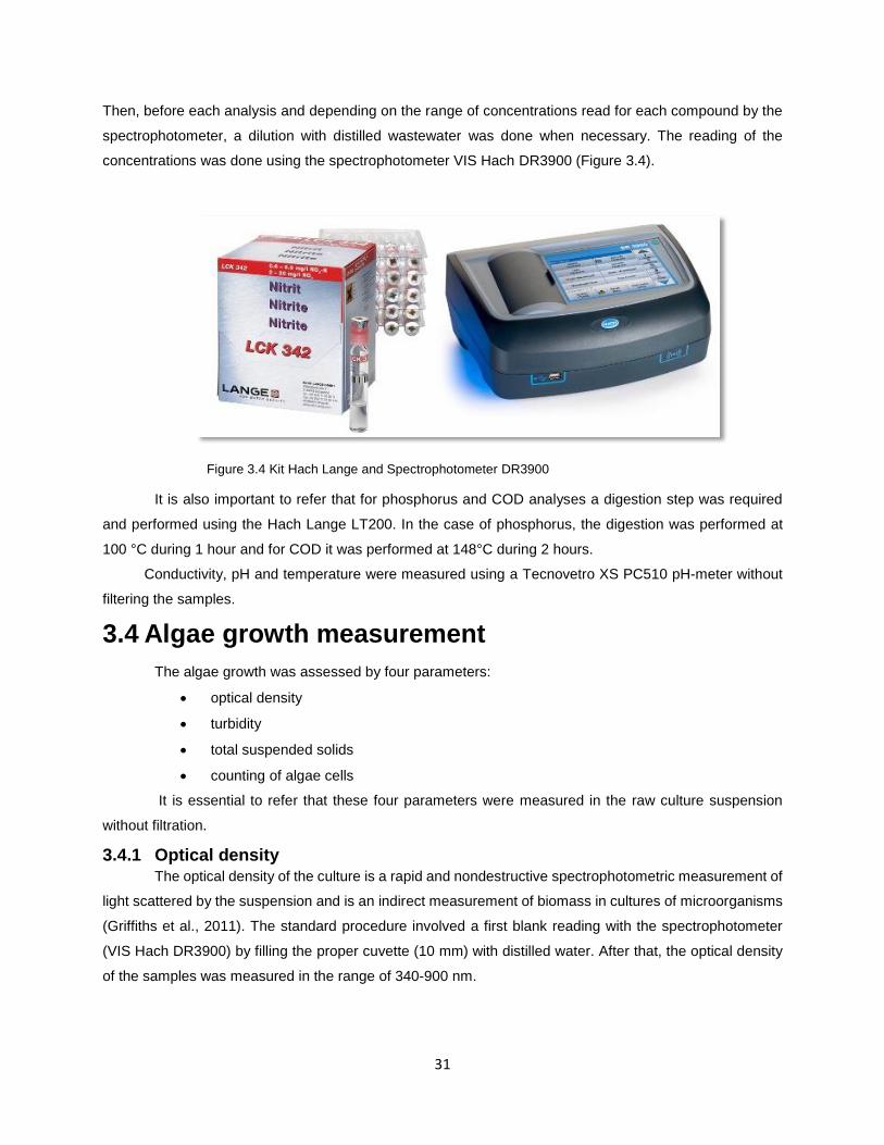
31
Then, before each analysis and depending on the range of concentrations read for each compound by the
spectrophotometer, a dilution with distilled wastewater was done when necessary. The reading of the
concentrations was done using the spectrophotometer VIS Hach DR3900 (Figure 3.4).
Figure 3.4 Kit Hach Lange and Spectrophotometer DR3900
It is also important to refer that for phosphorus and COD analyses a digestion step was required
and performed using the Hach Lange LT200. In the case of phosphorus, the digestion was performed at
100 °C during 1 hour and for COD it was performed at 148°C during 2 hours.
Conductivity, pH and temperature were measured using a Tecnovetro XS PC510 pH-meter without
filtering the samples.
3.4 Algae growth measurement
The algae growth was assessed by four parameters:
optical density
turbidity
total suspended solids
counting of algae cells
It is essential to refer that these four parameters were measured in the raw culture suspension
without filtration.
3.4.1 Optical density The optical density of the culture is a rapid and nondestructive spectrophotometric measurement of
light scattered by the suspension and is an indirect measurement of biomass in cultures of microorganisms
(Griffiths et al., 2011). The standard procedure involved a first blank reading with the spectrophotometer
(VIS Hach DR3900) by filling the proper cuvette (10 mm) with distilled water. After that, the optical density
of the samples was measured in the range of 340-900 nm.
32
In the determination of the optical density, when the values obtained were higher than 1, it was
necessary to do a dilution of the sample with distilled water since the values read by the spectrophotometer
are more precise when lower than 1.
Regarding the more accurate wavelength to use, there is little consensus about which value to use
in microalgae suspensions. However, the use of a wavelength between 650-680 nm has been reported to
correspond to the maximum absorbance value since it corresponds to the maximum absorbance of
chlorophyll (Griffiths et al., 2011). Figure 3.5 reports an example of a spectrum at different wavelengths and
it is possible to observe that the maximum absorbance in the visible range corresponds to 680 nm.
Figure 3.5 Example of a curve obtained from the measurement of absorbance at different wavelengths
3.4.2 Turbidty Turbidity is an optical determination of liquid clarity and is an expression of the amount of light that
is scattered by the suspension when a light is shined through the sample. Turbidity is an important water
quality parameter that detects the presence of suspend solids like algae.
The turbidity measurement was carried out by spectrophotometer (840 nm) and, as for the optical
density, the standard procedure started with a blank reading. For this parameter, a 5 cm cuvette was used
and usually, since the range of turbidity values read by the spectrophotometer was between 40-400 FAU, it
was necessary to dilute the samples with distilled water.
3.4.3 Total suspended solids The parameter total suspended solids is also important for the assessment of algae growth and
corresponds to a laboratory gravimetric procedure where the solids from the culture are filtered through a
47 cm glass fiber filter (1.2 µm porosity) (Sartorius stedim biotech).
The first step for the determination of TSS consisted in placing the filters in the oven (MPM
Instruments, type M80-VF) for 3 hours at 105 °C. Then, the filters were placed in a dryer and two hours
later, they were weighted in a balance (Acculab) .Then, 10 mL samples from each vial were filtered with
the aid of a vacuum pump (KNF NEUBERGER, D-79112). Finally, the filters were dried and weighed using
the procedure described previously.
0.0
0.5
1.0
1.5
2.0
2.5
3.0
3.5
34
03
67
39
44
21
44
84
75
50
25
29
55
65
83
61
06
37
66
46
91
71
87
45
77
27
99
82
68
53
88
0
OD
Wavelenght (nm)
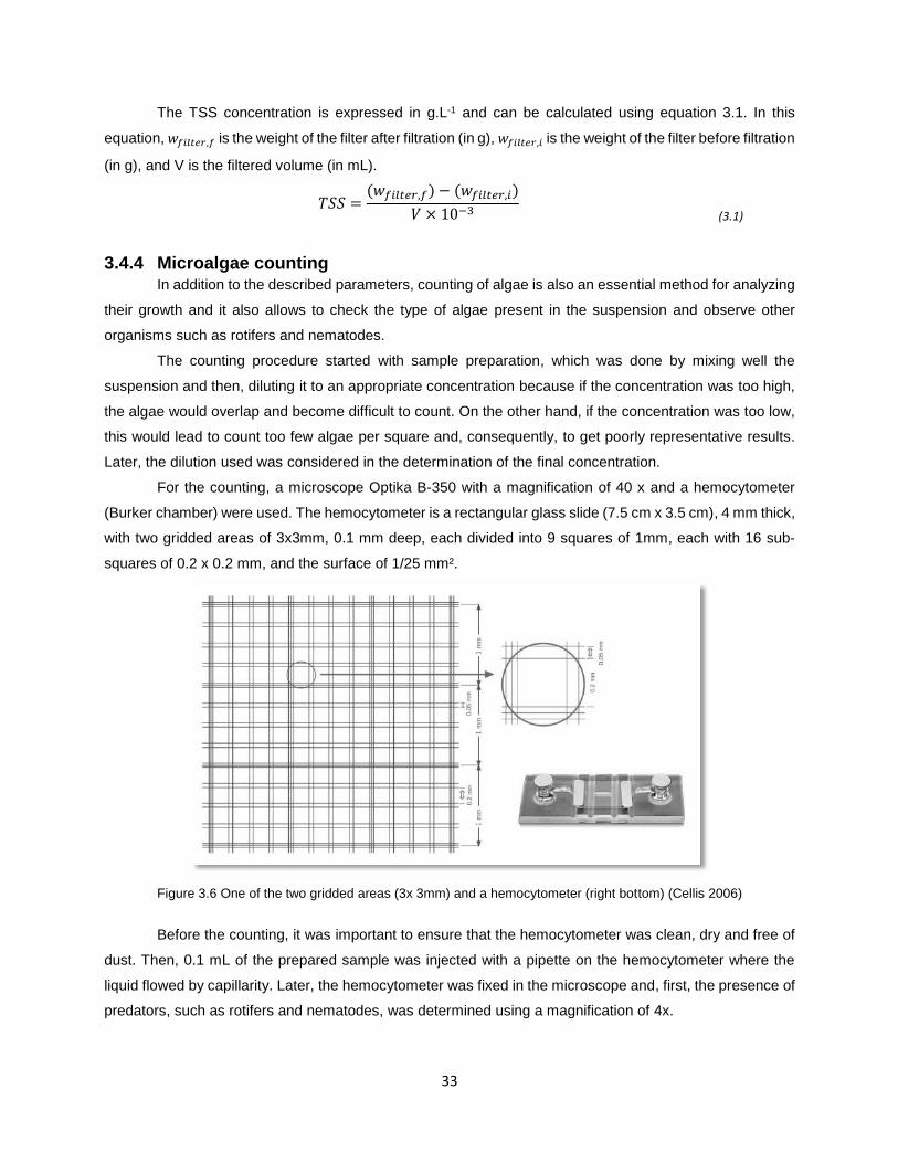
33
The TSS concentration is expressed in g.L-1 and can be calculated using equation 3.1. In this
equation, 𝑤𝑓𝑖𝑙𝑡𝑒𝑟,𝑓 is the weight of the filter after filtration (in g), 𝑤𝑓𝑖𝑙𝑡𝑒𝑟,𝑖 is the weight of the filter before filtration
(in g), and V is the filtered volume (in mL).
𝑇𝑆𝑆 =(𝑤𝑓𝑖𝑙𝑡𝑒𝑟,𝑓) − (𝑤𝑓𝑖𝑙𝑡𝑒𝑟,𝑖)
𝑉 × 10−3
(3.1)
3.4.4 Microalgae counting In addition to the described parameters, counting of algae is also an essential method for analyzing
their growth and it also allows to check the type of algae present in the suspension and observe other
organisms such as rotifers and nematodes.
The counting procedure started with sample preparation, which was done by mixing well the
suspension and then, diluting it to an appropriate concentration because if the concentration was too high,
the algae would overlap and become difficult to count. On the other hand, if the concentration was too low,
this would lead to count too few algae per square and, consequently, to get poorly representative results.
Later, the dilution used was considered in the determination of the final concentration.
For the counting, a microscope Optika B-350 with a magnification of 40 x and a hemocytometer
(Burker chamber) were used. The hemocytometer is a rectangular glass slide (7.5 cm x 3.5 cm), 4 mm thick,
with two gridded areas of 3x3mm, 0.1 mm deep, each divided into 9 squares of 1mm, each with 16 sub-
squares of 0.2 x 0.2 mm, and the surface of 1/25 mm².
Figure 3.6 One of the two gridded areas (3x 3mm) and a hemocytometer (right bottom) (Cellis 2006)
Before the counting, it was important to ensure that the hemocytometer was clean, dry and free of
dust. Then, 0.1 mL of the prepared sample was injected with a pipette on the hemocytometer where the
liquid flowed by capillarity. Later, the hemocytometer was fixed in the microscope and, first, the presence of
predators, such as rotifers and nematodes, was determined using a magnification of 4x.
34
After that, the counting of algae was done with a magnification of 40 x. During the first days of the
experiment the counting was only performed on 9 little squares (0.04 m2), randomly chosen. However, after
40 days for vial 1 and 2 and 29 days for vial A and B, the count was extended to 36 little squares in the
bottom part of the hemocytometer and 36 in the top one, each square with 0.04 mm2, in order to obtain
more reliable data. In each big square, 3 lines were randomly chosen, each with 12 squares.
Another important rule involved in the counting was that the algae that were on the line of a grid
that touch the bottom and the right lines of a square should not be counted. On the contrary, cells on the
top and left side should be counted.
Finally, the concentration of algae, expressed in cell.mL-1, was determined using the equation 3.2,
where the volume of the square is expressed in mL. Since the considered squares have 0.04 mm2 surface,
the volume of the square is 0.000004 mL.
𝐶𝑒𝑙𝑙𝑐𝑜𝑛𝑐𝑒𝑛𝑡𝑟𝑎𝑡𝑖𝑜𝑛 = (𝑛𝑢𝑚𝑏𝑒𝑟 𝑜𝑓 𝑐𝑒𝑙𝑙𝑠 𝑐𝑜𝑢𝑛𝑡𝑒𝑑
𝑛𝑢𝑚𝑏𝑒𝑟 𝑜𝑓 𝑠𝑞𝑢𝑎𝑟𝑒𝑠)(
𝑑𝑖𝑙𝑢𝑡𝑖𝑜𝑛
𝑣𝑜𝑙𝑢𝑚𝑒 𝑜𝑓 𝑡ℎ𝑒 𝑠𝑞𝑢𝑎𝑟𝑒) (3.2)
3.5 Experimental procedure
The analyses of all the previously described parameters were performed 3 times per week. Each
day, before starting the analyses, distilled water was added to the four vials in order to compensate the
evaporated water. Then, 5 mL of suspension from each vial were filtered on 47 glass fiber filter (Sartorius
stedim biotech) and the concentration of N-NH₄⁺;P-PO₄³⁻;N-NO₂⁻;N-NO₃⁻ and COD (in mg.L-1) were
determined on the filtered samples.
The turbidity was determined using 1 mL of suspension, without filtering, and diluting it with distilled
water. In addition, optical density, pH, conductivity and temperature were also measured.
If the concentration of ammonium nitrogen was lower than 100 mg.L-1, a mass balance was done
to determine the volume of wastewater which had to be replaced in the vials in order to ensure that the
concentration of ammonium nitrogen inside each vial was maintained around 200 mg.L-1.
The calculations used to determine the volume of wastewater necessary to add (Vadd) are
represented in equation 3.3 and 3.4.
First, the mass of ammonium nitrogen which should be added (madd) was calculated by equation
3.3, where[𝑁 − 𝑁𝐻4]𝑜𝑏𝑗 is the objective concentration of ammonium nitrogen inside the vial; Vvial is the
volume of each vial in L (0.150 L for each vial); [𝑁 − 𝑁𝐻4]𝑚𝑒𝑎𝑠 is the measured concentration of ammonium
nitrogen in mg.L-1 ; 𝑉𝑣𝑖𝑎𝑙,𝑑 is the volume of the vial in the day of analyses.
Then, knowing the concentration of ammonium nitrogen in the wastewater ([𝑁𝐻4]𝑊𝑊1) that is
expressed in mg.L-1, it was possible to determine the Vadd.
𝑚𝑎𝑑𝑑 = [𝑁 − 𝑁𝐻4]𝑜𝑏𝑗 × 𝑉𝑣𝑖𝑎𝑙 − [𝑁 − 𝑁𝐻4]𝑚𝑒𝑎𝑠 × 𝑉𝑣𝑖𝑎𝑙,𝑑 (3.3)
35
𝑉 𝑎𝑑𝑑 =𝑚𝑎𝑑𝑑
[𝑁 − 𝑁𝐻4]𝑊𝑊1
(3.4)
Every time the addition of wastewater was necessary, all the analyses were repeated later and the
TSS (mg.L-1) were measured following the procedure described in chapter 3.4.3.
After the addition of wastewater, it was important to check if N/P was lower than 10. Otherwise, a 2
g.L-1 solution of Na2HPO4 was added to the vials to keep the ratio lower or equal to 10.
Algae counts were only performed before addition, following the procedure described in chapter
3.4.4.
3.6 Respirometric tests
As it was already discussed, microalgae are able to remove inorganic nitrogen from wastewaters.
However, part of ammonium nitrogen is removed by nitrifying bacteria, which require the oxygen produced
by microalgae during photosynthesis and therefore, establishing a symbiotic relation with microalgae
(Muñoz & Guieysse, 2006). Normally, the nitrification process mediated by bacteria involves two steps,
ammonium oxidation into nitrite by a group of bacteria and nitrite oxidation into nitrate by other bacteria
group (Tilley, 2011).
Respirometry is the measurement of the respiration rate of organisms and is defined as the amount
of oxygen per unit of volume and time that is consumed by the microorganisms. Respirometric tests allow
to plot oxygen concentration against time and the rate of oxygen consumption can be obtained by calculating
the slope in that time (Nollet & Gelder, 2014).
The aim of performing respirometric analyses was to confirm the presence of other microorganisms
besides microalgae and to measure the uptake of oxygen by three different organisms which could be
present in the culture suspension: AOB; NOB and heterotrophic organisms (HO).
In order to analyze separately the different activities present in this mixed culture containing
microalgae, selective inhibitors were used taking into account that the inhibition should be instantaneous
and complete for the target population and not affect other populations. Therefore, allythiourea (ATU)
(Ginestet et al., 1998) was used to inhibit AOB and potassium chlorate (Hynes & Knowles, 1983) for
inhibiting NOB , without affecting any other populations.
The respirometric test was performed using a suspension obtained by taking 20 mL of each vial (1,
2, A and B) and mixing it in just one vial. Then, it was added wastewater WW1 until reaching 100 mL of
volume and the vial was aerated and exposed to light in the same conditions described in 3.2.1 chapter. In
addition, the vial was fed following the normal procedure described in chapter 3.5, during one week, with
the aim of adapting and growing more microalgae.
Sodium nitrite and ammonium chloride were added with the aim of ensuring that ammonia and nitrite
nitrogen concentrations were not limiting during the experiment. Besides, a solution of sodium acetate was
also prepared to be used as a substrate for heterotrophic organisms. Thus, in order to prepare these
solutions it was necessary to do calculations taking into account the need for 10 mg.L-1 of N-NO-2,10 mg.L-
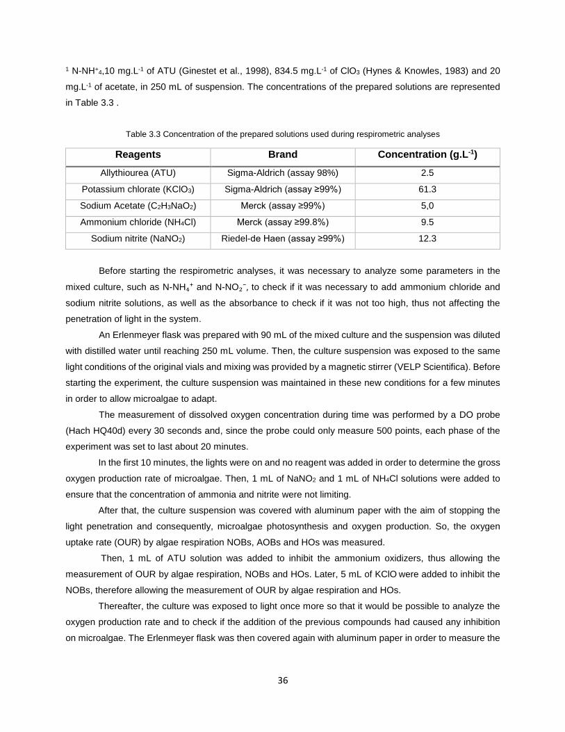
36
1 N-NH+4,10 mg.L-1 of ATU (Ginestet et al., 1998), 834.5 mg.L-1 of ClO3 (Hynes & Knowles, 1983) and 20
mg.L-1 of acetate, in 250 mL of suspension. The concentrations of the prepared solutions are represented
in Table 3.3 .
Table 3.3 Concentration of the prepared solutions used during respirometric analyses
Reagents Brand Concentration (g.L-1)
Allythiourea (ATU) Sigma-Aldrich (assay 98%) 2.5
Potassium chlorate (KClO3) Sigma-Aldrich (assay ≥99%) 61.3
Sodium Acetate (C2H3NaO2) Merck (assay ≥99%) 5,0
Ammonium chloride (NH4Cl) Merck (assay ≥99.8%) 9.5
Sodium nitrite (NaNO2) Riedel-de Haen (assay ≥99%) 12.3
Before starting the respirometric analyses, it was necessary to analyze some parameters in the
mixed culture, such as N-NH₄⁺ and N-NO₂⁻, to check if it was necessary to add ammonium chloride and
sodium nitrite solutions, as well as the absorbance to check if it was not too high, thus not affecting the
penetration of light in the system.
An Erlenmeyer flask was prepared with 90 mL of the mixed culture and the suspension was diluted
with distilled water until reaching 250 mL volume. Then, the culture suspension was exposed to the same
light conditions of the original vials and mixing was provided by a magnetic stirrer (VELP Scientifica). Before
starting the experiment, the culture suspension was maintained in these new conditions for a few minutes
in order to allow microalgae to adapt.
The measurement of dissolved oxygen concentration during time was performed by a DO probe
(Hach HQ40d) every 30 seconds and, since the probe could only measure 500 points, each phase of the
experiment was set to last about 20 minutes.
In the first 10 minutes, the lights were on and no reagent was added in order to determine the gross
oxygen production rate of microalgae. Then, 1 mL of NaNO2 and 1 mL of NH4Cl solutions were added to
ensure that the concentration of ammonia and nitrite were not limiting.
After that, the culture suspension was covered with aluminum paper with the aim of stopping the
light penetration and consequently, microalgae photosynthesis and oxygen production. So, the oxygen
uptake rate (OUR) by algae respiration NOBs, AOBs and HOs was measured.
Then, 1 mL of ATU solution was added to inhibit the ammonium oxidizers, thus allowing the
measurement of OUR by algae respiration, NOBs and HOs. Later, 5 mL of KClO were added to inhibit the
NOBs, therefore allowing the measurement of OUR by algae respiration and HOs.
Thereafter, the culture was exposed to light once more so that it would be possible to analyze the
oxygen production rate and to check if the addition of the previous compounds had caused any inhibition
on microalgae. The Erlenmeyer flask was then covered again with aluminum paper in order to measure the
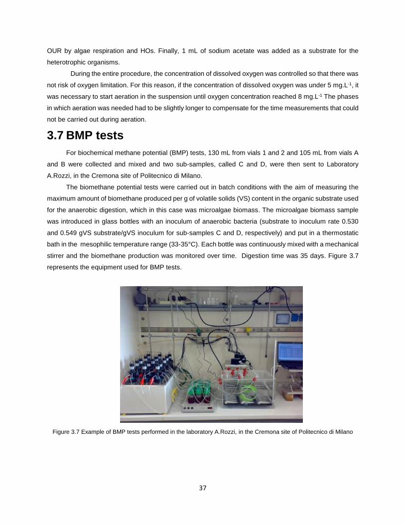
37
OUR by algae respiration and HOs. Finally, 1 mL of sodium acetate was added as a substrate for the
heterotrophic organisms.
During the entire procedure, the concentration of dissolved oxygen was controlled so that there was
not risk of oxygen limitation. For this reason, if the concentration of dissolved oxygen was under 5 mg.L-1, it
was necessary to start aeration in the suspension until oxygen concentration reached 8 mg.L-1 The phases
in which aeration was needed had to be slightly longer to compensate for the time measurements that could
not be carried out during aeration.
3.7 BMP tests
For biochemical methane potential (BMP) tests, 130 mL from vials 1 and 2 and 105 mL from vials A
and B were collected and mixed and two sub-samples, called C and D, were then sent to Laboratory
A.Rozzi, in the Cremona site of Politecnico di Milano.
The biomethane potential tests were carried out in batch conditions with the aim of measuring the
maximum amount of biomethane produced per g of volatile solids (VS) content in the organic substrate used
for the anaerobic digestion, which in this case was microalgae biomass. The microalgae biomass sample
was introduced in glass bottles with an inoculum of anaerobic bacteria (substrate to inoculum rate 0.530
and 0.549 gVS substrate/gVS inoculum for sub-samples C and D, respectively) and put in a thermostatic
bath in the mesophilic temperature range (33-35°C). Each bottle was continuously mixed with a mechanical
stirrer and the biomethane production was monitored over time. Digestion time was 35 days. Figure 3.7
represents the equipment used for BMP tests.
Figure 3.7 Example of BMP tests performed in the laboratory A.Rozzi, in the Cremona site of Politecnico di Milano
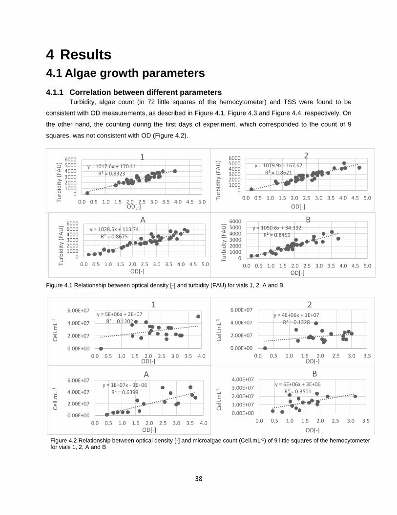
38
4 Results
4.1 Algae growth parameters
4.1.1 Correlation between different parameters Turbidity, algae count (in 72 little squares of the hemocytometer) and TSS were found to be
consistent with OD measurements, as described in Figure 4.1, Figure 4.3 and Figure 4.4, respectively. On
the other hand, the counting during the first days of experiment, which corresponded to the count of 9
squares, was not consistent with OD (Figure 4.2).
y = 1079.9x - 167.62R² = 0.8621
0100020003000400050006000
0.0 0.5 1.0 1.5 2.0 2.5 3.0 3.5 4.0 4.5 5.0Turb
idit
y (F
AU
)
OD[-]
2y = 1017.6x + 170.11
R² = 0.8323
0100020003000400050006000
0.0 0.5 1.0 1.5 2.0 2.5 3.0 3.5 4.0 4.5 5.0Turb
idit
y (F
AU
)
OD[-]
1
y = 1028.5x + 113.74R² = 0.8675
0100020003000400050006000
0.0 0.5 1.0 1.5 2.0 2.5 3.0 3.5 4.0 4.5 5.0Turb
idit
y (F
AU
)
OD[-]
Ay = 1050.6x + 34.332
R² = 0.8459
0100020003000400050006000
0.0 0.5 1.0 1.5 2.0 2.5 3.0 3.5 4.0 4.5 5.0
Turb
idty
(FA
U)
OD[-]
B
Figure 4.1 Relationship between optical density [-] and turbidity (FAU) for vials 1, 2, A and B
y = 5E+06x + 2E+07R² = 0.1202
0.00E+00
2.00E+07
4.00E+07
6.00E+07
0.0 0.5 1.0 1.5 2.0 2.5 3.0 3.5 4.0
Cel
l.mL-1
OD[-]
1y = 4E+06x + 1E+07
R² = 0.1228
0.00E+00
2.00E+07
4.00E+07
6.00E+07
0.0 0.5 1.0 1.5 2.0 2.5 3.0 3.5
Cel
l.mL-1
OD[-]
2
y = 1E+07x - 3E+06R² = 0.6399
0.00E+00
2.00E+07
4.00E+07
6.00E+07
0.0 0.5 1.0 1.5 2.0 2.5 3.0 3.5 4.0
Cel
l.mL-1
OD[-]
Ay = 6E+06x + 3E+06
R² = 0.3501
0.00E+00
1.00E+07
2.00E+07
3.00E+07
4.00E+07
0.0 0.5 1.0 1.5 2.0 2.5 3.0 3.5
Cel
l.mL-1
OD[-]
B
Figure 4.2 Relationship between optical density [-] and microalgae count (Cell.mL-1) of 9 little squares of the hemocytometer for vials 1, 2, A and B
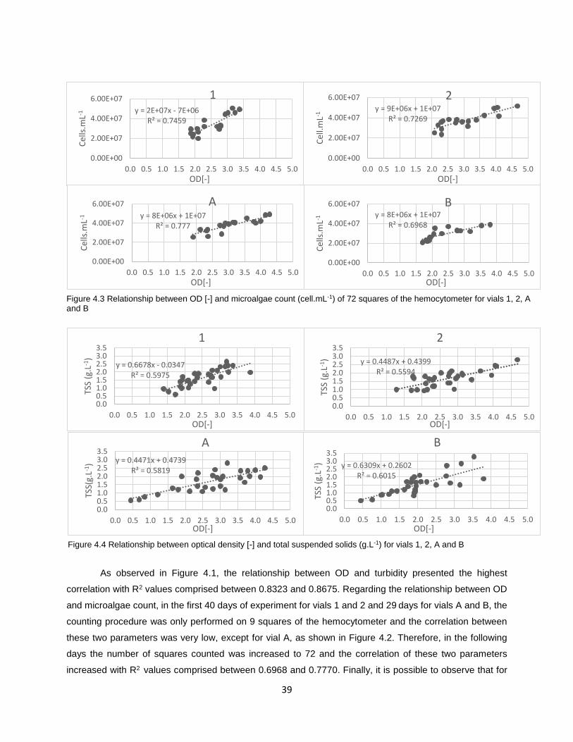
39
As observed in Figure 4.1, the relationship between OD and turbidity presented the highest
correlation with R2 values comprised between 0.8323 and 0.8675. Regarding the relationship between OD
and microalgae count, in the first 40 days of experiment for vials 1 and 2 and 29 days for vials A and B, the
counting procedure was only performed on 9 squares of the hemocytometer and the correlation between
these two parameters was very low, except for vial A, as shown in Figure 4.2. Therefore, in the following
days the number of squares counted was increased to 72 and the correlation of these two parameters
increased with R2 values comprised between 0.6968 and 0.7770. Finally, it is possible to observe that for
y = 2E+07x - 7E+06R² = 0.7459
0.00E+00
2.00E+07
4.00E+07
6.00E+07
0.0 0.5 1.0 1.5 2.0 2.5 3.0 3.5 4.0 4.5 5.0
Cel
ls.m
L-1
OD[-]
1y = 9E+06x + 1E+07
R² = 0.7269
0.00E+00
2.00E+07
4.00E+07
6.00E+07
0.0 0.5 1.0 1.5 2.0 2.5 3.0 3.5 4.0 4.5 5.0
Cel
l.mL-1
OD[-]
2
y = 8E+06x + 1E+07R² = 0.6968
0.00E+00
2.00E+07
4.00E+07
6.00E+07
0.0 0.5 1.0 1.5 2.0 2.5 3.0 3.5 4.0 4.5 5.0
Cel
ls.m
L-1
OD[-]
By = 8E+06x + 1E+07
R² = 0.777
0.00E+00
2.00E+07
4.00E+07
6.00E+07
0.0 0.5 1.0 1.5 2.0 2.5 3.0 3.5 4.0 4.5 5.0
Cel
ls.m
L-1
OD[-]
A
y = 0.4487x + 0.4399R² = 0.5594
0.00.51.01.52.02.53.03.5
0.0 0.5 1.0 1.5 2.0 2.5 3.0 3.5 4.0 4.5 5.0
TSS
(g.L
-1)
OD[-]
2
y = 0.6678x - 0.0347R² = 0.5975
0.00.51.01.52.02.53.03.5
0.0 0.5 1.0 1.5 2.0 2.5 3.0 3.5 4.0 4.5 5.0
TSS
(g.L
-1)
OD[-]
1
y = 0.4471x + 0.4739R² = 0.5819
0.00.51.01.52.02.53.03.5
0.0 0.5 1.0 1.5 2.0 2.5 3.0 3.5 4.0 4.5 5.0
TSS(
g.L-1
)
OD[-]
A
y = 0.6309x + 0.2602R² = 0.6015
0.00.51.01.52.02.53.03.5
0.0 0.5 1.0 1.5 2.0 2.5 3.0 3.5 4.0 4.5 5.0
TSS
(g.L
-1)
OD[-]
B
Figure 4.3 Relationship between OD [-] and microalgae count (cell.mL-1) of 72 squares of the hemocytometer for vials 1, 2, A and B
Figure 4.4 Relationship between optical density [-] and total suspended solids (g.L-1) for vials 1, 2, A and B
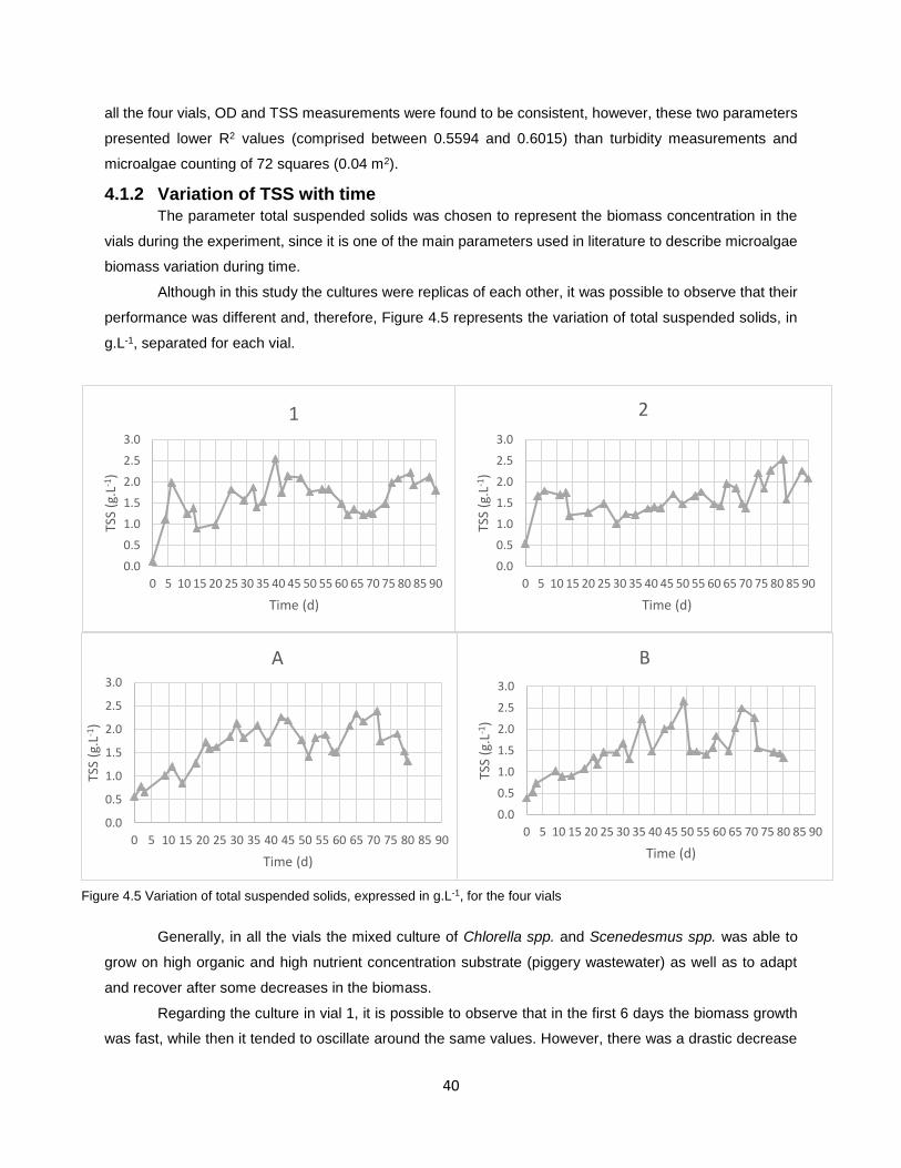
40
all the four vials, OD and TSS measurements were found to be consistent, however, these two parameters
presented lower R2 values (comprised between 0.5594 and 0.6015) than turbidity measurements and
microalgae counting of 72 squares (0.04 m2).
4.1.2 Variation of TSS with time The parameter total suspended solids was chosen to represent the biomass concentration in the
vials during the experiment, since it is one of the main parameters used in literature to describe microalgae
biomass variation during time.
Although in this study the cultures were replicas of each other, it was possible to observe that their
performance was different and, therefore, Figure 4.5 represents the variation of total suspended solids, in
g.L-1, separated for each vial.
Generally, in all the vials the mixed culture of Chlorella spp. and Scenedesmus spp. was able to
grow on high organic and high nutrient concentration substrate (piggery wastewater) as well as to adapt
and recover after some decreases in the biomass.
Regarding the culture in vial 1, it is possible to observe that in the first 6 days the biomass growth
was fast, while then it tended to oscillate around the same values. However, there was a drastic decrease
0.0
0.5
1.0
1.5
2.0
2.5
3.0
0 5 10 15 20 25 30 35 40 45 50 55 60 65 70 75 80 85 90
TSS
(g.L
-1)
Time (d)
1
0.0
0.5
1.0
1.5
2.0
2.5
3.0
0 5 10 15 20 25 30 35 40 45 50 55 60 65 70 75 80 85 90
TSS
(g.L
-1)
Time (d)
2
0.0
0.5
1.0
1.5
2.0
2.5
3.0
0 5 10 15 20 25 30 35 40 45 50 55 60 65 70 75 80 85 90
TSS
(g.L
-1)
Time (d)
A
0.0
0.5
1.0
1.5
2.0
2.5
3.0
0 5 10 15 20 25 30 35 40 45 50 55 60 65 70 75 80 85 90
TSS
(g.L
-1)
Time (d)
B
Figure 4.5 Variation of total suspended solids, expressed in g.L-1, for the four vials
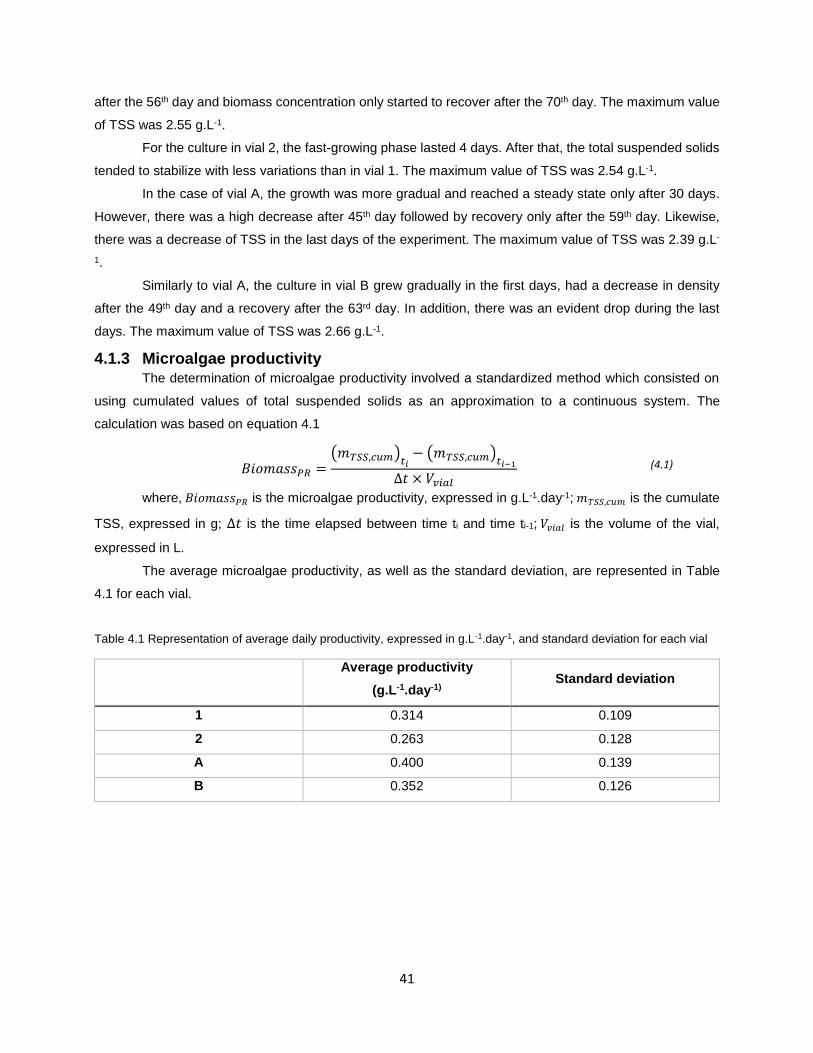
41
after the 56th day and biomass concentration only started to recover after the 70th day. The maximum value
of TSS was 2.55 g.L-1.
For the culture in vial 2, the fast-growing phase lasted 4 days. After that, the total suspended solids
tended to stabilize with less variations than in vial 1. The maximum value of TSS was 2.54 g.L-1.
In the case of vial A, the growth was more gradual and reached a steady state only after 30 days.
However, there was a high decrease after 45th day followed by recovery only after the 59th day. Likewise,
there was a decrease of TSS in the last days of the experiment. The maximum value of TSS was 2.39 g.L-
1.
Similarly to vial A, the culture in vial B grew gradually in the first days, had a decrease in density
after the 49th day and a recovery after the 63rd day. In addition, there was an evident drop during the last
days. The maximum value of TSS was 2.66 g.L-1.
4.1.3 Microalgae productivity The determination of microalgae productivity involved a standardized method which consisted on
using cumulated values of total suspended solids as an approximation to a continuous system. The
calculation was based on equation 4.1
𝐵𝑖𝑜𝑚𝑎𝑠𝑠𝑃𝑅 =(𝑚𝑇𝑆𝑆,𝑐𝑢𝑚)𝑡𝑖
− (𝑚𝑇𝑆𝑆,𝑐𝑢𝑚)𝑡𝑖−1∆𝑡 × 𝑉𝑣𝑖𝑎𝑙
(4.1)
where, 𝐵𝑖𝑜𝑚𝑎𝑠𝑠𝑃𝑅 is the microalgae productivity, expressed in g.L-1.day-1; 𝑚𝑇𝑆𝑆,𝑐𝑢𝑚 is the cumulate
TSS, expressed in g; ∆𝑡 is the time elapsed between time ti and time ti-1; 𝑉𝑣𝑖𝑎𝑙 is the volume of the vial,
expressed in L.
The average microalgae productivity, as well as the standard deviation, are represented in Table
4.1 for each vial.
Table 4.1 Representation of average daily productivity, expressed in g.L-1.day-1, and standard deviation for each vial
Average productivity
(g.L-1.day-1) Standard deviation
1 0.314 0.109
2 0.263 0.128
A 0.400 0.139
B 0.352 0.126
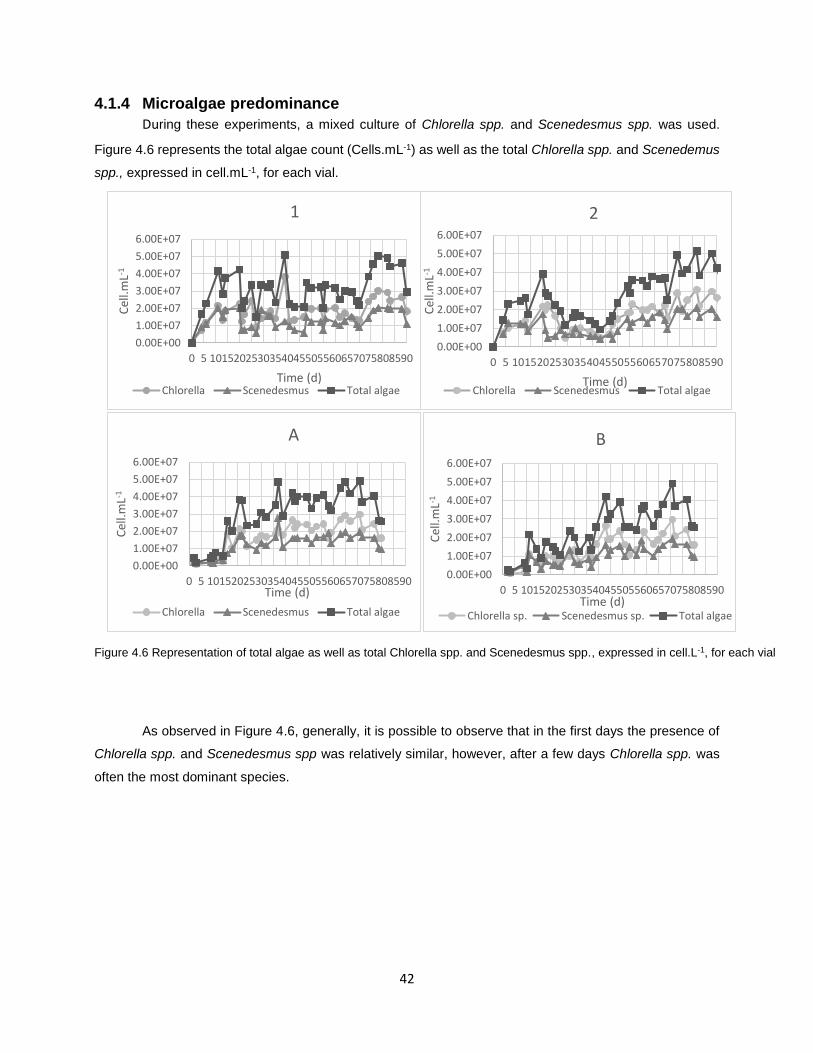
42
4.1.4 Microalgae predominance
During these experiments, a mixed culture of Chlorella spp. and Scenedesmus spp. was used.
Figure 4.6 represents the total algae count (Cells.mL-1) as well as the total Chlorella spp. and Scenedemus
spp., expressed in cell.mL-1, for each vial.
As observed in Figure 4.6, generally, it is possible to observe that in the first days the presence of
Chlorella spp. and Scenedesmus spp was relatively similar, however, after a few days Chlorella spp. was
often the most dominant species.
Figure 4.6 Representation of total algae as well as total Chlorella spp. and Scenedesmus spp., expressed in cell.L-1, for each vial
0.00E+00
1.00E+07
2.00E+07
3.00E+07
4.00E+07
5.00E+07
6.00E+07
0 5 1015202530354045505560657075808590
Cel
l.mL-1
Time (d)
2
Chlorella Scenedesmus Total algae
0.00E+00
1.00E+07
2.00E+07
3.00E+07
4.00E+07
5.00E+07
6.00E+07
0 5 1015202530354045505560657075808590
Cel
l.mL-1
Time (d)
1
Chlorella Scenedesmus Total algae
0.00E+00
1.00E+07
2.00E+07
3.00E+07
4.00E+07
5.00E+07
6.00E+07
0 5 1015202530354045505560657075808590
Cel
l.mL-1
Time (d)
A
Chlorella Scenedesmus Total algae
0.00E+00
1.00E+07
2.00E+07
3.00E+07
4.00E+07
5.00E+07
6.00E+07
0 5 1015202530354045505560657075808590
Cel
l.mL-1
Time (d)
B
Chlorella sp. Scenedesmus sp. Total algae
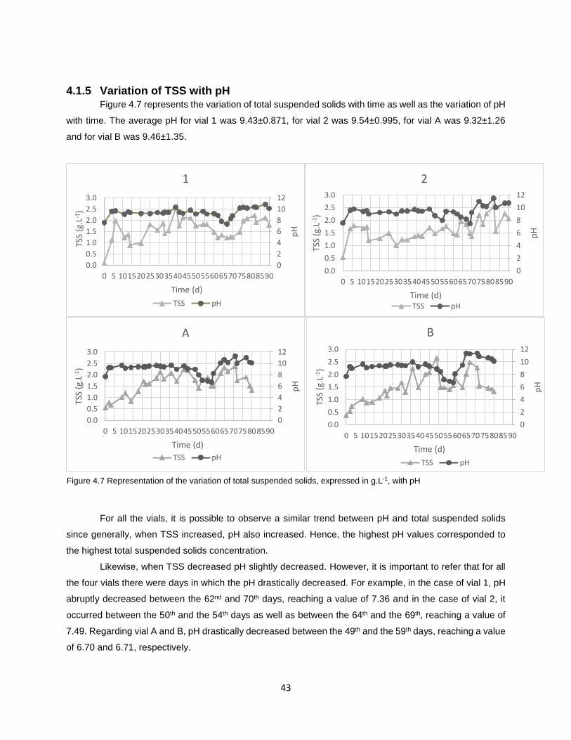
43
4.1.5 Variation of TSS with pH Figure 4.7 represents the variation of total suspended solids with time as well as the variation of pH
with time. The average pH for vial 1 was 9.43±0.871, for vial 2 was 9.54±0.995, for vial A was 9.32±1.26
and for vial B was 9.46±1.35.
For all the vials, it is possible to observe a similar trend between pH and total suspended solids
since generally, when TSS increased, pH also increased. Hence, the highest pH values corresponded to
the highest total suspended solids concentration.
Likewise, when TSS decreased pH slightly decreased. However, it is important to refer that for all
the four vials there were days in which the pH drastically decreased. For example, in the case of vial 1, pH
abruptly decreased between the 62nd and 70th days, reaching a value of 7.36 and in the case of vial 2, it
occurred between the 50th and the 54th days as well as between the 64th and the 69th, reaching a value of
7.49. Regarding vial A and B, pH drastically decreased between the 49th and the 59th days, reaching a value
of 6.70 and 6.71, respectively.
0
2
4
6
8
10
12
0.0
0.5
1.0
1.5
2.0
2.5
3.0
0 5 1015202530354045505560657075808590
pH
TSS
(g.L
-1)
Time (d)
1
TSS pH
0
2
4
6
8
10
12
0.0
0.5
1.0
1.5
2.0
2.5
3.0
0 5 1015202530354045505560657075808590
pH
TSS
(g.L
-1)
Time (d)
2
TSS pH
0
2
4
6
8
10
12
0.0
0.5
1.0
1.5
2.0
2.5
3.0
0 5 1015202530354045505560657075808590
pH
TSS
(g.L
-1)
Time (d)
A
TSS pH
0
2
4
6
8
10
12
0.0
0.5
1.0
1.5
2.0
2.5
3.0
0 5 1015202530354045505560657075808590
pH
TSS
(g.L
-1)
Time (d)
B
TSS pH
Figure 4.7 Representation of the variation of total suspended solids, expressed in g.L-1, with pH
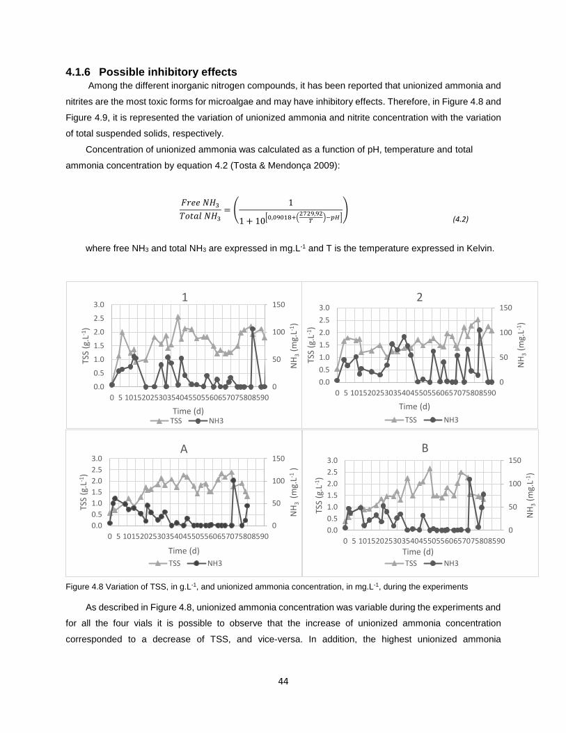
44
4.1.6 Possible inhibitory effects Among the different inorganic nitrogen compounds, it has been reported that unionized ammonia and
nitrites are the most toxic forms for microalgae and may have inhibitory effects. Therefore, in Figure 4.8 and
Figure 4.9, it is represented the variation of unionized ammonia and nitrite concentration with the variation
of total suspended solids, respectively.
Concentration of unionized ammonia was calculated as a function of pH, temperature and total
ammonia concentration by equation 4.2 (Tosta & Mendonça 2009):
𝐹𝑟𝑒𝑒 𝑁𝐻3𝑇𝑜𝑡𝑎𝑙 𝑁𝐻3
= (1
1 + 10[0,09018+(2729,92𝑇
)−𝑝𝐻])
(4.2)
where free NH3 and total NH3 are expressed in mg.L-1 and T is the temperature expressed in Kelvin.
As described in Figure 4.8, unionized ammonia concentration was variable during the experiments and
for all the four vials it is possible to observe that the increase of unionized ammonia concentration
corresponded to a decrease of TSS, and vice-versa. In addition, the highest unionized ammonia
Figure 4.8 Variation of TSS, in g.L-1, and unionized ammonia concentration, in mg.L-1, during the experiments
0
50
100
150
0.0
0.5
1.0
1.5
2.0
2.5
3.0
0 5 1015202530354045505560657075808590
NH
3(m
g.L-1
)
TSS
(g.L
-1)
Time (d)
1
TSS NH3
0
50
100
150
0.0
0.5
1.0
1.5
2.0
2.5
3.0
0 5 1015202530354045505560657075808590
NH
3(m
g.L-1
)
TSS
(g.L
-1)
Time (d)
2
TSS NH3
0
50
100
150
0.0
0.5
1.0
1.5
2.0
2.5
3.0
0 5 1015202530354045505560657075808590
NH
3 (m
g.L-1
)
TSS
(g.L
-1)
Time (d)
A
TSS NH3
0
50
100
150
0.0
0.5
1.0
1.5
2.0
2.5
3.0
0 5 1015202530354045505560657075808590
NH
3(m
g.L-1
)
TSS
(g.L
-1)
Time (d)
B
TSS NH3
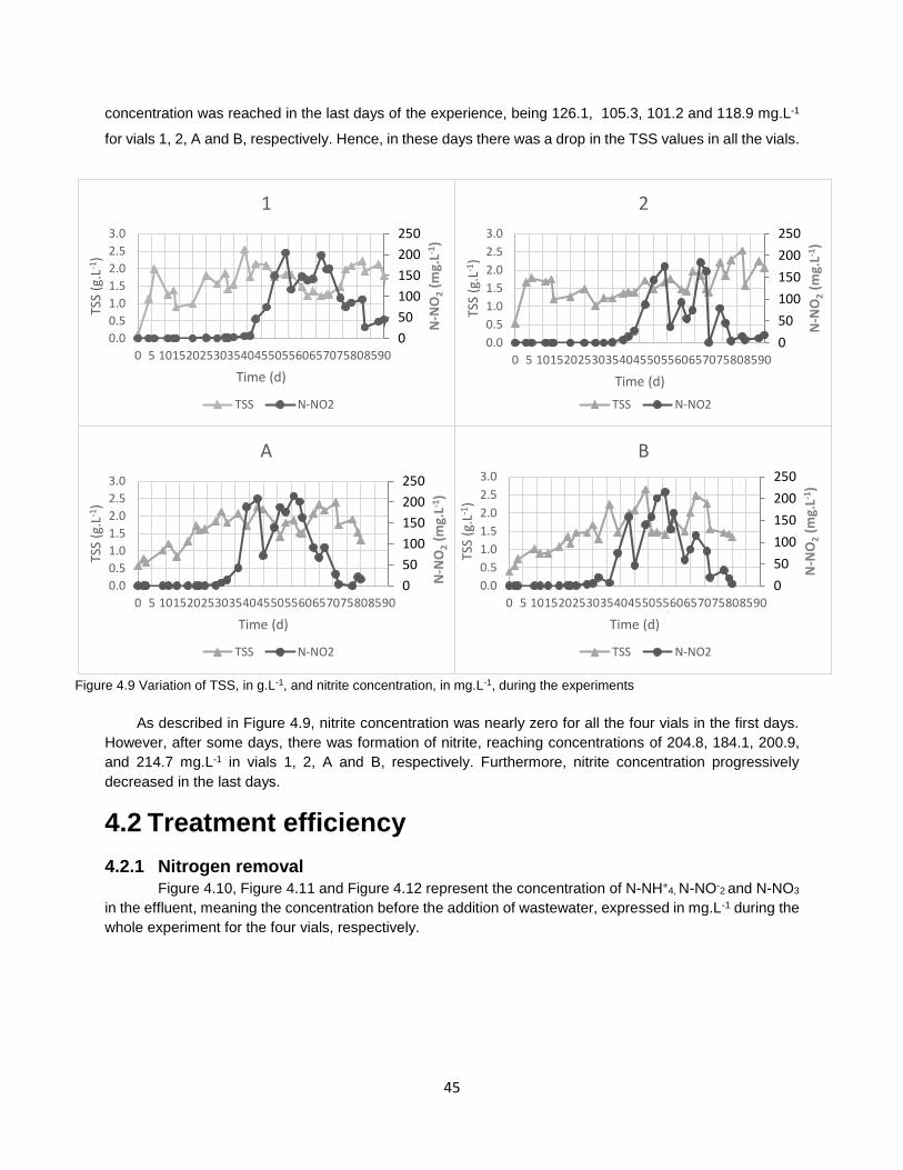
45
concentration was reached in the last days of the experience, being 126.1, 105.3, 101.2 and 118.9 mg.L-1
for vials 1, 2, A and B, respectively. Hence, in these days there was a drop in the TSS values in all the vials.
As described in Figure 4.9, nitrite concentration was nearly zero for all the four vials in the first days.
However, after some days, there was formation of nitrite, reaching concentrations of 204.8, 184.1, 200.9,
and 214.7 mg.L-1 in vials 1, 2, A and B, respectively. Furthermore, nitrite concentration progressively
decreased in the last days.
4.2 Treatment efficiency
4.2.1 Nitrogen removal
Figure 4.10, Figure 4.11 and Figure 4.12 represent the concentration of N-NH+4, N-NO-
2 and N-NO3
in the effluent, meaning the concentration before the addition of wastewater, expressed in mg.L-1 during the
whole experiment for the four vials, respectively.
Figure 4.9 Variation of TSS, in g.L-1, and nitrite concentration, in mg.L-1, during the experiments
0
50
100
150
200
250
0.0
0.5
1.0
1.5
2.0
2.5
3.0
0 5 1015202530354045505560657075808590
N-N
O2
(mg.
L-1)
TSS
(g.L
-1)
Time (d)
2
TSS N-NO2
0
50
100
150
200
250
0.0
0.5
1.0
1.5
2.0
2.5
3.0
0 5 1015202530354045505560657075808590
N-N
O2
(mg.
L-1)
TSS
(g.L
-1)
Time (d)
1
TSS N-NO2
0
50
100
150
200
250
0.0
0.5
1.0
1.5
2.0
2.5
3.0
0 5 1015202530354045505560657075808590
N-N
O2
(mg.
L-1)
TSS
(g.L
-1)
Time (d)
A
TSS N-NO2
0
50
100
150
200
250
0.0
0.5
1.0
1.5
2.0
2.5
3.0
0 5 1015202530354045505560657075808590
N-N
O2
(mg.
L-1)
TSS
(g.L
-1)
Time (d)
B
TSS N-NO2
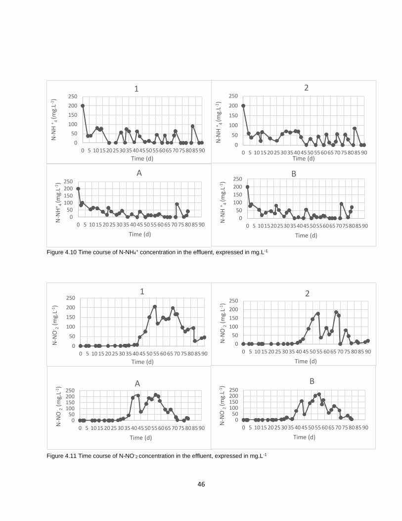
46
Figure 4.10 Time course of N-NH4+ concentration in the effluent, expressed in mg.L-1
0
50
100
150
200
250
0 5 10 15 20 25 30 35 40 45 50 55 60 65 70 75 80 85 90
N-N
O- 2
(mg.
L-1)
Time (d)
1
0
50
100
150
200
250
0 5 10 15 20 25 30 35 40 45 50 55 60 65 70 75 80 85 90
N-N
O- 2
(mg.
L-1)
Time (d)
2
050
100150200250
0 5 10 15 20 25 30 35 40 45 50 55 60 65 70 75 80 85 90
N-N
O- 2
(mg.
L-1)
Time (d)
A
050
100150200250
0 5 10 15 20 25 30 35 40 45 50 55 60 65 70 75 80 85 90
N-N
O- 2
(mg.
L-1)
Time (d)
B
Figure 4.11 Time course of N-NO-2 concentration in the effluent, expressed in mg.L-1
0
50
100
150
200
250
0 5 10 15 20 25 30 35 40 45 50 55 60 65 70 75 80 85 90
N-N
H + 4
(mg.
L-1)
Time (d)
2
0
50
100
150
200
250
0 5 1015202530354045505560657075808590
N-N
H +
4 (m
g.L-1
)
Time (d)
1
050
100150200250
0 5 10 15 20 25 30 35 40 45 50 55 60 65 70 75 80 85 90
N-N
H+
4 (m
g.L-1
)
Time (d)
A
0
50
100
150
200
250
0 5 1015202530354045505560657075808590N
-NH
+4
(mg.
L-1)
Time (d)
B
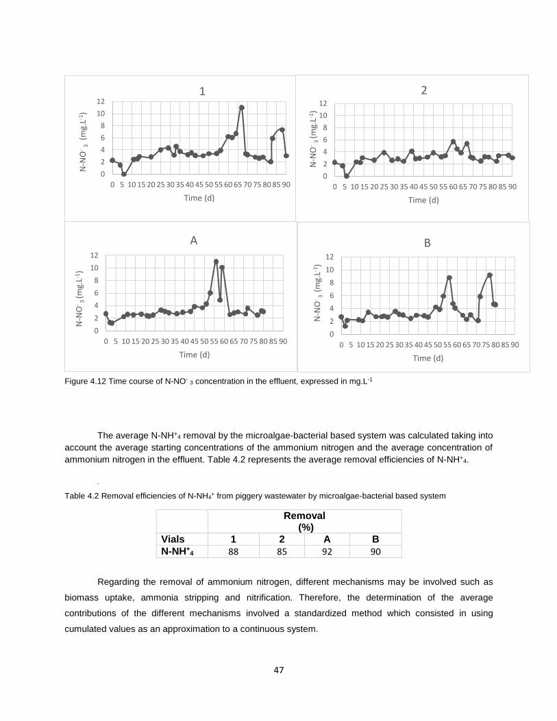
47
The average N-NH+4 removal by the microalgae-bacterial based system was calculated taking into
account the average starting concentrations of the ammonium nitrogen and the average concentration of
ammonium nitrogen in the effluent. Table 4.2 represents the average removal efficiencies of N-NH+4.
.
Table 4.2 Removal efficiencies of N-NH4+ from piggery wastewater by microalgae-bacterial based system
Removal (%)
Vials 1 2 A B
N-NH+4 88 85 92 90
Regarding the removal of ammonium nitrogen, different mechanisms may be involved such as
biomass uptake, ammonia stripping and nitrification. Therefore, the determination of the average
contributions of the different mechanisms involved a standardized method which consisted in using
cumulated values as an approximation to a continuous system.
0
2
4
6
8
10
12
0 5 10 15 20 25 30 35 40 45 50 55 60 65 70 75 80 85 90
N-N
O-
3(m
g.L-1
)
Time (d)
1
0
2
4
6
8
10
12
0 5 10 15 20 25 30 35 40 45 50 55 60 65 70 75 80 85 90
N-N
O-
3 (m
g.L-1
)
Time (d)
2
0
2
4
6
8
10
12
0 5 10 15 20 25 30 35 40 45 50 55 60 65 70 75 80 85 90
N-N
O-
3 (m
g.L-1
)
Time (d)
A
0
2
4
6
8
10
12
0 5 10 15 20 25 30 35 40 45 50 55 60 65 70 75 80 85 90
N-N
O-
3 (
mg.
L-1)
Time (d)
B
Figure 4.12 Time course of N-NO- 3 concentration in the effluent, expressed in mg.L-1
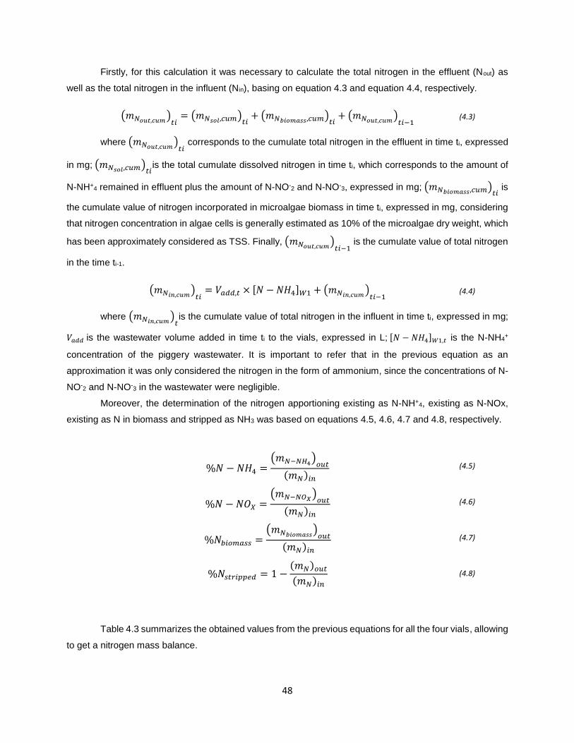
48
Firstly, for this calculation it was necessary to calculate the total nitrogen in the effluent (Nout) as
well as the total nitrogen in the influent (Nin), basing on equation 4.3 and equation 4.4, respectively.
(𝑚𝑁𝑜𝑢𝑡,𝑐𝑢𝑚)𝑡𝑖= (𝑚𝑁𝑠𝑜𝑙,𝑐𝑢𝑚)𝑡𝑖
+ (𝑚𝑁𝑏𝑖𝑜𝑚𝑎𝑠𝑠,𝑐𝑢𝑚)𝑡𝑖+ (𝑚𝑁𝑜𝑢𝑡,𝑐𝑢𝑚)𝑡𝑖−1
(4.3)
where (𝑚𝑁𝑜𝑢𝑡,𝑐𝑢𝑚)𝑡𝑖 corresponds to the cumulate total nitrogen in the effluent in time ti, expressed
in mg; (𝑚𝑁𝑠𝑜𝑙,𝑐𝑢𝑚)𝑡𝑖is the total cumulate dissolved nitrogen in time ti, which corresponds to the amount of
N-NH+4 remained in effluent plus the amount of N-NO-
2 and N-NO-3, expressed in mg; (𝑚𝑁𝑏𝑖𝑜𝑚𝑎𝑠𝑠,𝑐𝑢𝑚)𝑡𝑖
is
the cumulate value of nitrogen incorporated in microalgae biomass in time ti, expressed in mg, considering
that nitrogen concentration in algae cells is generally estimated as 10% of the microalgae dry weight, which
has been approximately considered as TSS. Finally, (𝑚𝑁𝑜𝑢𝑡,𝑐𝑢𝑚)𝑡𝑖−1 is the cumulate value of total nitrogen
in the time ti-1.
(𝑚𝑁𝑖𝑛,𝑐𝑢𝑚)𝑡𝑖= 𝑉𝑎𝑑𝑑,𝑡 × [𝑁 − 𝑁𝐻4]𝑊1 + (𝑚𝑁𝑖𝑛,𝑐𝑢𝑚)𝑡𝑖−1
(4.4)
where (𝑚𝑁𝑖𝑛,𝑐𝑢𝑚)𝑡is the cumulate value of total nitrogen in the influent in time ti, expressed in mg;
𝑉𝑎𝑑𝑑 is the wastewater volume added in time ti to the vials, expressed in L; [𝑁 − 𝑁𝐻4]𝑊1,𝑡 is the N-NH4+
concentration of the piggery wastewater. It is important to refer that in the previous equation as an
approximation it was only considered the nitrogen in the form of ammonium, since the concentrations of N-
NO-2 and N-NO-
3 in the wastewater were negligible.
Moreover, the determination of the nitrogen apportioning existing as N-NH+4, existing as N-NOx,
existing as N in biomass and stripped as NH3 was based on equations 4.5, 4.6, 4.7 and 4.8, respectively.
%𝑁 −𝑁𝐻4 =(𝑚𝑁−𝑁𝐻4)𝑜𝑢𝑡(𝑚𝑁)𝑖𝑛
(4.5)
%𝑁 −𝑁𝑂𝑋 =(𝑚𝑁−𝑁𝑂𝑋)𝑜𝑢𝑡(𝑚𝑁)𝑖𝑛
(4.6)
%𝑁𝑏𝑖𝑜𝑚𝑎𝑠𝑠 =(𝑚𝑁𝑏𝑖𝑜𝑚𝑎𝑠𝑠)𝑜𝑢𝑡(𝑚𝑁)𝑖𝑛
(4.7)
%𝑁𝑠𝑡𝑟𝑖𝑝𝑝𝑒𝑑 = 1 −(𝑚𝑁)𝑜𝑢𝑡(𝑚𝑁)𝑖𝑛
(4.8)
Table 4.3 summarizes the obtained values from the previous equations for all the four vials, allowing
to get a nitrogen mass balance.
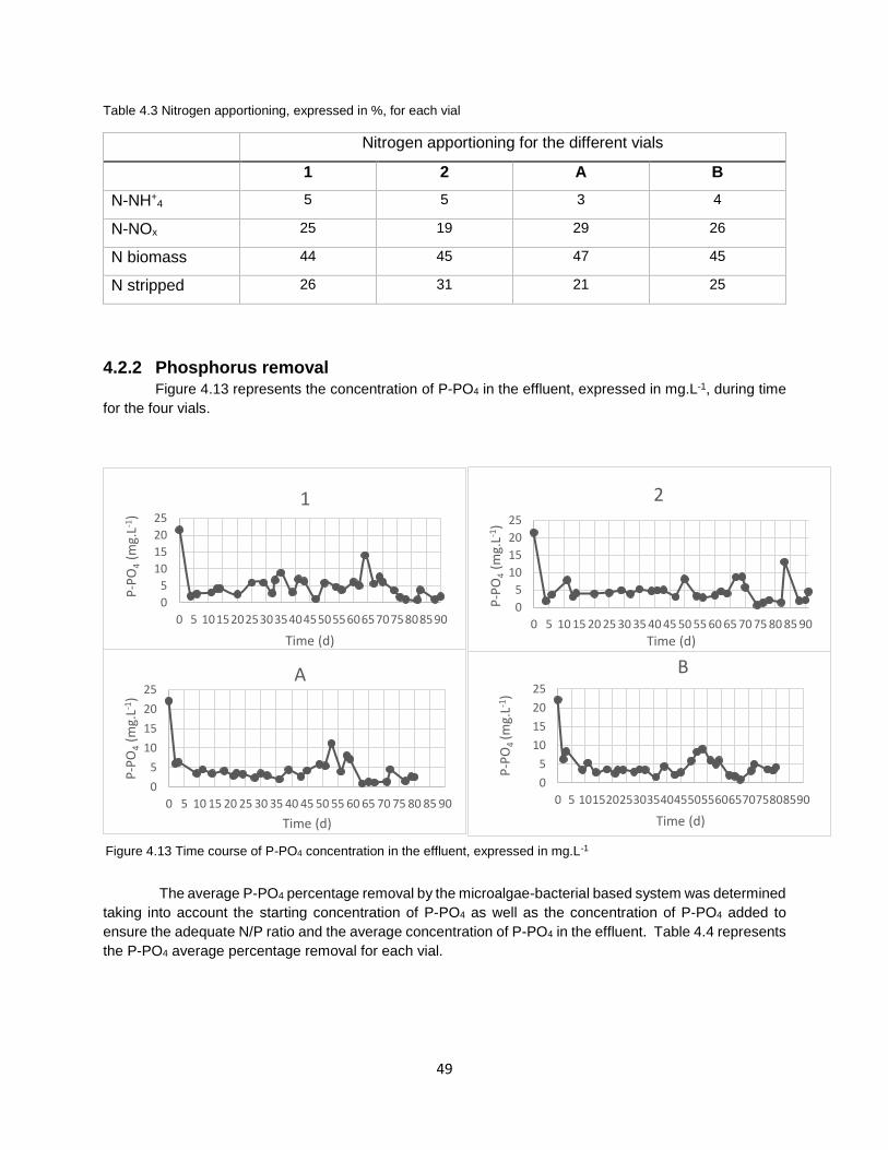
49
Table 4.3 Nitrogen apportioning, expressed in %, for each vial
Nitrogen apportioning for the different vials
1 2 A B
N-NH+4 5 5 3 4
N-NOx 25 19 29 26
N biomass 44 45 47 45
N stripped 26 31 21 25
4.2.2 Phosphorus removal
Figure 4.13 represents the concentration of P-PO4 in the effluent, expressed in mg.L-1, during time
for the four vials.
The average P-PO4 percentage removal by the microalgae-bacterial based system was determined
taking into account the starting concentration of P-PO4 as well as the concentration of P-PO4 added to
ensure the adequate N/P ratio and the average concentration of P-PO4 in the effluent. Table 4.4 represents
the P-PO4 average percentage removal for each vial.
Figure 4.13 Time course of P-PO4 concentration in the effluent, expressed in mg.L-1
0
5
10
15
20
25
0 5 10 15 20 25 30 35 40 45 50 55 60 65 70 75 80 85 90
P-P
O4
(mg.
L-1)
Time (d)
2
0
5
10
15
20
25
0 5 1015202530354045505560657075808590
P-P
O4
(mg.
L-1)
Time (d)
1
0
5
10
15
20
25
0 5 10 15 20 25 30 35 40 45 50 55 60 65 70 75 80 85 90
P-P
O4
(mg.
L-1)
Time (d)
A
0
5
10
15
20
25
0 5 1015202530354045505560657075808590
P-P
O4
(mg.
L-1)
Time (d)
B
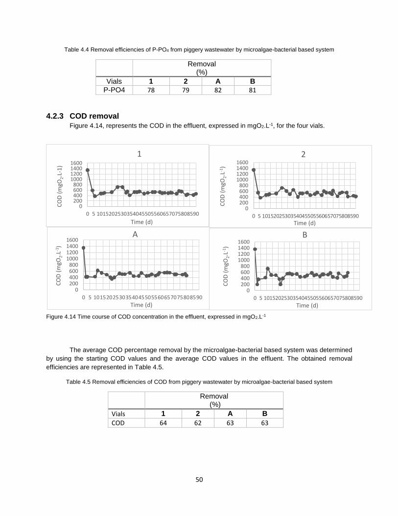
50
Table 4.4 Removal efficiencies of P-PO4 from piggery wastewater by microalgae-bacterial based system
Removal (%)
Vials 1 2 A B
P-PO4 78 79 82 81
4.2.3 COD removal Figure 4.14, represents the COD in the effluent, expressed in mgO2.L-1, for the four vials.
The average COD percentage removal by the microalgae-bacterial based system was determined
by using the starting COD values and the average COD values in the effluent. The obtained removal
efficiencies are represented in Table 4.5.
Table 4.5 Removal efficiencies of COD from piggery wastewater by microalgae-bacterial based system
Removal (%)
Vials 1 2 A B
COD 64 62 63 63
Figure 4.14 Time course of COD concentration in the effluent, expressed in mgO2.L-1
0200400600800
1000120014001600
0 5 1015202530354045505560657075808590C
OD
(m
gO2.
L-1)
Time (d)
2
0200400600800
1000120014001600
0 5 1015202530354045505560657075808590
CO
D (
mgO
2.L-
1)
Time (d)
1
0200400600800
1000120014001600
0 5 1015202530354045505560657075808590
CO
D (
mgO
2.L
-1)
Time (d)
A
0200400600800
1000120014001600
0 5 1015202530354045505560657075808590
CO
D (
mgO
2.L
-1)
Time (d)
B
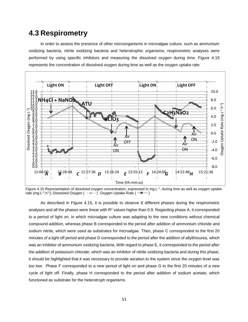
51
4.3 Respirometry
In order to assess the presence of other microorganisms in microalgae culture, such as ammonium
oxidizing bacteria, nitrite oxidizing bacteria and heterotrophic organisms, respirometric analyses were
performed by using specific inhibitors and measuring the dissolved oxygen during time. Figure 4.15
represents the concentration of dissolved oxygen during time as well as the oxygen uptake rate.
As described in Figure 4.15, it is possible to observe 8 different phases during the respirometric
analyses and all the phases were linear with R2 values higher than 0.9. Regarding phase A, it corresponded
to a period of light on, in which microalgae culture was adapting to the new conditions without chemical
compound addition, whereas phase B corresponded to the period after addition of ammonium chloride and
sodium nitrite, which were used as substrates for microalgae. Then, phase C corresponded to the first 20
minutes of a light off period and phase D corresponded to the period after the addition of allylthiourea, which
was an inhibitor of ammonium oxidizing bacteria. With regard to phase E, it corresponded to the period after
the addition of potassium chlorate, which was an inhibitor of nitrite oxidizing bacteria and during this phase,
it should be highlighted that it was necessary to provide aeration to the system since the oxygen level was
too low. Phase F corresponded to a new period of light on and phase G to the first 20 minutes of a new
cycle of light off. Finally, phase H corresponded to the period after addition of sodium acetate, which
functioned as substrate for the heterotroph organisms.
-8.0
-6.0
-4.0
-2.0
0.0
2.0
4.0
6.0
8.0
10.0
0.00.51.01.52.02.53.03.54.04.55.05.56.06.57.07.58.08.59.09.5
10.010.511.011.512.012.513.0
12:00:00 12:28:48 12:57:36 13:26:24 13:55:12 14:24:00 14:52:48 15:21:36
Oxy
gen
Up
take
Rat
e (m
g L-1
h-1
)
Dis
solv
ed O
xyge
n (
mg
L-1)
Time (hh:mm:ss)
Light ON Light OFF Light ON Light OFF
NH4Cl + NaNO2ATU
KClO3C2H3NaO2
AirON
AirON
AirON
AirOFF
A B C D E F G H
Figure 4.15 Representation of dissolved oxygen concentration, expressed in mg.L-1, during time as well as oxygen uptake rate (mg.L-1.h-1); Dissolved Oxygen ( ) Oxygen Uptake Rate ( )
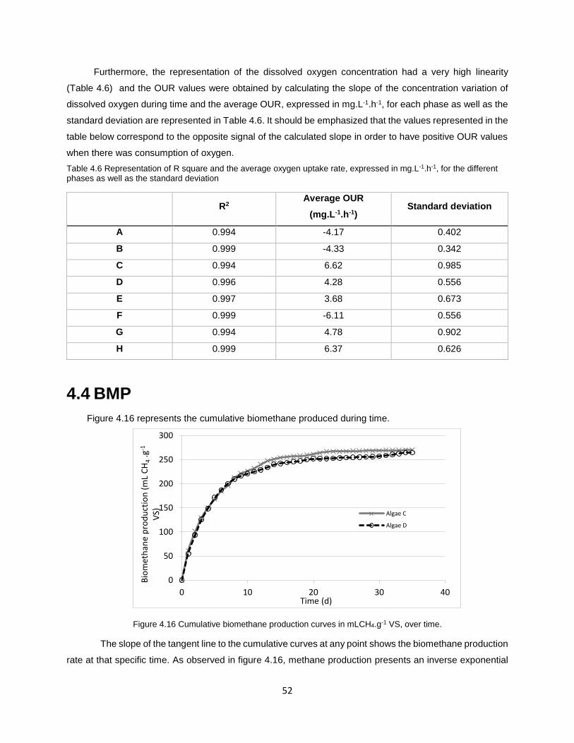
52
Furthermore, the representation of the dissolved oxygen concentration had a very high linearity
(Table 4.6) and the OUR values were obtained by calculating the slope of the concentration variation of
dissolved oxygen during time and the average OUR, expressed in mg.L-1.h-1, for each phase as well as the
standard deviation are represented in Table 4.6. It should be emphasized that the values represented in the
table below correspond to the opposite signal of the calculated slope in order to have positive OUR values
when there was consumption of oxygen.
Table 4.6 Representation of R square and the average oxygen uptake rate, expressed in mg.L-1.h-1, for the different phases as well as the standard deviation
R2 Average OUR
(mg.L-1.h-1) Standard deviation
A 0.994 -4.17 0.402
B 0.999 -4.33 0.342
C 0.994 6.62 0.985
D 0.996 4.28 0.556
E 0.997 3.68 0.673
F 0.999 -6.11 0.556
G 0.994 4.78 0.902
H 0.999 6.37 0.626
4.4 BMP
Figure 4.16 represents the cumulative biomethane produced during time.
Figure 4.16 Cumulative biomethane production curves in mLCH4.g-1 VS, over time.
The slope of the tangent line to the cumulative curves at any point shows the biomethane production
rate at that specific time. As observed in figure 4.16, methane production presents an inverse exponential
0
50
100
150
200
250
300
0 10 20 30 40
Bio
met
han
e p
rod
uct
ion
(m
L C
H4
.g-1
VS)
Time (d)
Algae C
Algae D

53
curve that is characterized by three main zones. During the initial phase there was a rapid biomethane
production, which slows down during the intermediate phase and tend to zero at the end of the final phase.
Furthermore, both algae cultures had a similar curve and the maximum methane production was 270.4
and 264.3 mLCH4.g-1 VS for algae C and D, respectively.
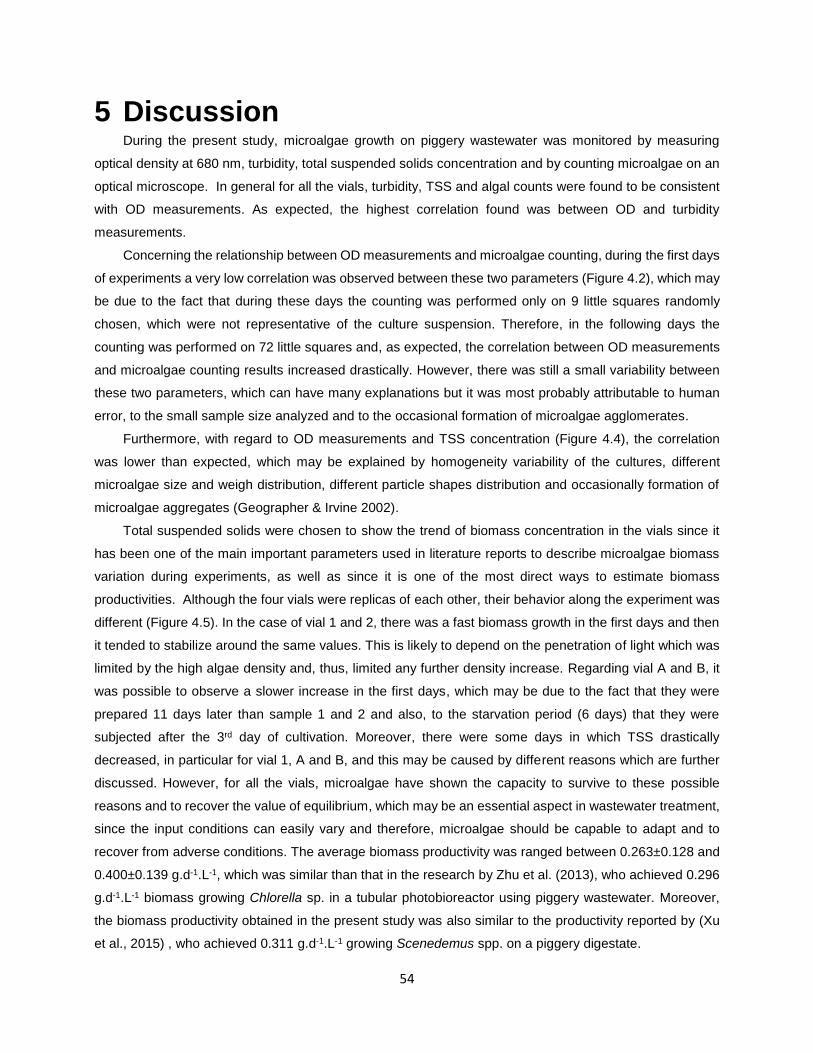
54
5 Discussion During the present study, microalgae growth on piggery wastewater was monitored by measuring
optical density at 680 nm, turbidity, total suspended solids concentration and by counting microalgae on an
optical microscope. In general for all the vials, turbidity, TSS and algal counts were found to be consistent
with OD measurements. As expected, the highest correlation found was between OD and turbidity
measurements.
Concerning the relationship between OD measurements and microalgae counting, during the first days
of experiments a very low correlation was observed between these two parameters (Figure 4.2), which may
be due to the fact that during these days the counting was performed only on 9 little squares randomly
chosen, which were not representative of the culture suspension. Therefore, in the following days the
counting was performed on 72 little squares and, as expected, the correlation between OD measurements
and microalgae counting results increased drastically. However, there was still a small variability between
these two parameters, which can have many explanations but it was most probably attributable to human
error, to the small sample size analyzed and to the occasional formation of microalgae agglomerates.
Furthermore, with regard to OD measurements and TSS concentration (Figure 4.4), the correlation
was lower than expected, which may be explained by homogeneity variability of the cultures, different
microalgae size and weigh distribution, different particle shapes distribution and occasionally formation of
microalgae aggregates (Geographer & Irvine 2002).
Total suspended solids were chosen to show the trend of biomass concentration in the vials since it
has been one of the main important parameters used in literature reports to describe microalgae biomass
variation during experiments, as well as since it is one of the most direct ways to estimate biomass
productivities. Although the four vials were replicas of each other, their behavior along the experiment was
different (Figure 4.5). In the case of vial 1 and 2, there was a fast biomass growth in the first days and then
it tended to stabilize around the same values. This is likely to depend on the penetration of light which was
limited by the high algae density and, thus, limited any further density increase. Regarding vial A and B, it
was possible to observe a slower increase in the first days, which may be due to the fact that they were
prepared 11 days later than sample 1 and 2 and also, to the starvation period (6 days) that they were
subjected after the 3rd day of cultivation. Moreover, there were some days in which TSS drastically
decreased, in particular for vial 1, A and B, and this may be caused by different reasons which are further
discussed. However, for all the vials, microalgae have shown the capacity to survive to these possible
reasons and to recover the value of equilibrium, which may be an essential aspect in wastewater treatment,
since the input conditions can easily vary and therefore, microalgae should be capable to adapt and to
recover from adverse conditions. The average biomass productivity was ranged between 0.263±0.128 and
0.400±0.139 g.d-1.L-1, which was similar than that in the research by Zhu et al. (2013), who achieved 0.296
g.d-1.L-1 biomass growing Chlorella sp. in a tubular photobioreactor using piggery wastewater. Moreover,
the biomass productivity obtained in the present study was also similar to the productivity reported by (Xu
et al., 2015) , who achieved 0.311 g.d-1.L-1 growing Scenedemus spp. on a piggery digestate.
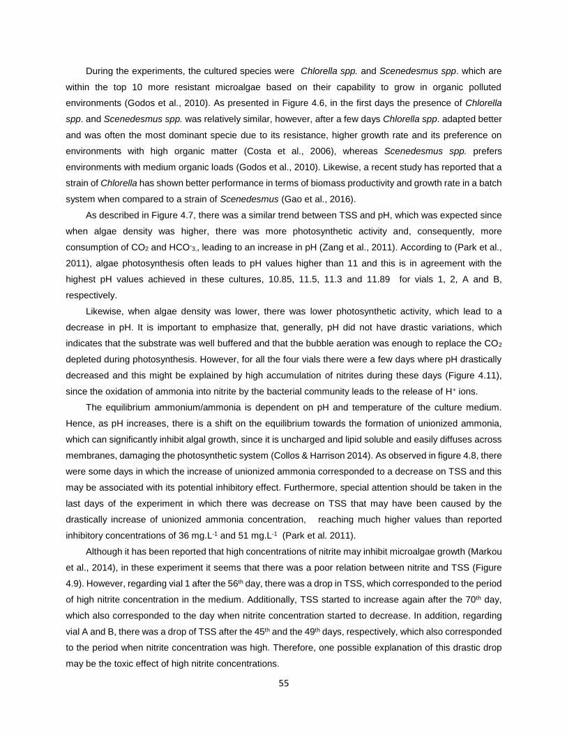
55
During the experiments, the cultured species were Chlorella spp. and Scenedesmus spp. which are
within the top 10 more resistant microalgae based on their capability to grow in organic polluted
environments (Godos et al., 2010). As presented in Figure 4.6, in the first days the presence of Chlorella
spp. and Scenedesmus spp. was relatively similar, however, after a few days Chlorella spp. adapted better
and was often the most dominant specie due to its resistance, higher growth rate and its preference on
environments with high organic matter (Costa et al., 2006), whereas Scenedesmus spp. prefers
environments with medium organic loads (Godos et al., 2010). Likewise, a recent study has reported that a
strain of Chlorella has shown better performance in terms of biomass productivity and growth rate in a batch
system when compared to a strain of Scenedesmus (Gao et al., 2016).
As described in Figure 4.7, there was a similar trend between TSS and pH, which was expected since
when algae density was higher, there was more photosynthetic activity and, consequently, more
consumption of CO2 and HCO-3,, leading to an increase in pH (Zang et al., 2011). According to (Park et al.,
2011), algae photosynthesis often leads to pH values higher than 11 and this is in agreement with the
highest pH values achieved in these cultures, 10.85, 11.5, 11.3 and 11.89 for vials 1, 2, A and B,
respectively.
Likewise, when algae density was lower, there was lower photosynthetic activity, which lead to a
decrease in pH. It is important to emphasize that, generally, pH did not have drastic variations, which
indicates that the substrate was well buffered and that the bubble aeration was enough to replace the CO2
depleted during photosynthesis. However, for all the four vials there were a few days where pH drastically
decreased and this might be explained by high accumulation of nitrites during these days (Figure 4.11),
since the oxidation of ammonia into nitrite by the bacterial community leads to the release of H+ ions.
The equilibrium ammonium/ammonia is dependent on pH and temperature of the culture medium.
Hence, as pH increases, there is a shift on the equilibrium towards the formation of unionized ammonia,
which can significantly inhibit algal growth, since it is uncharged and lipid soluble and easily diffuses across
membranes, damaging the photosynthetic system (Collos & Harrison 2014). As observed in figure 4.8, there
were some days in which the increase of unionized ammonia corresponded to a decrease on TSS and this
may be associated with its potential inhibitory effect. Furthermore, special attention should be taken in the
last days of the experiment in which there was decrease on TSS that may have been caused by the
drastically increase of unionized ammonia concentration, reaching much higher values than reported
inhibitory concentrations of 36 mg.L-1 and 51 mg.L-1 (Park et al. 2011).
Although it has been reported that high concentrations of nitrite may inhibit microalgae growth (Markou
et al., 2014), in these experiment it seems that there was a poor relation between nitrite and TSS (Figure
4.9). However, regarding vial 1 after the 56th day, there was a drop in TSS, which corresponded to the period
of high nitrite concentration in the medium. Additionally, TSS started to increase again after the 70th day,
which also corresponded to the day when nitrite concentration started to decrease. In addition, regarding
vial A and B, there was a drop of TSS after the 45th and the 49th days, respectively, which also corresponded
to the period when nitrite concentration was high. Therefore, one possible explanation of this drastic drop
may be the toxic effect of high nitrite concentrations.
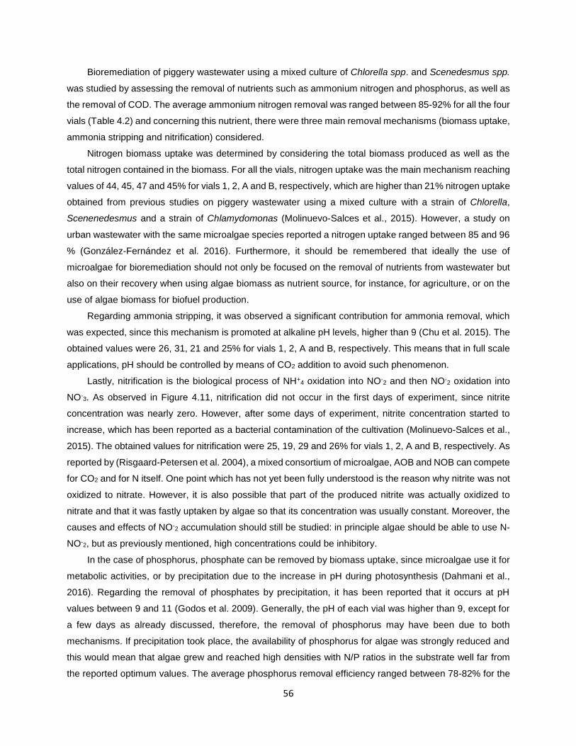
56
Bioremediation of piggery wastewater using a mixed culture of Chlorella spp. and Scenedesmus spp.
was studied by assessing the removal of nutrients such as ammonium nitrogen and phosphorus, as well as
the removal of COD. The average ammonium nitrogen removal was ranged between 85-92% for all the four
vials (Table 4.2) and concerning this nutrient, there were three main removal mechanisms (biomass uptake,
ammonia stripping and nitrification) considered.
Nitrogen biomass uptake was determined by considering the total biomass produced as well as the
total nitrogen contained in the biomass. For all the vials, nitrogen uptake was the main mechanism reaching
values of 44, 45, 47 and 45% for vials 1, 2, A and B, respectively, which are higher than 21% nitrogen uptake
obtained from previous studies on piggery wastewater using a mixed culture with a strain of Chlorella,
Scenenedesmus and a strain of Chlamydomonas (Molinuevo-Salces et al., 2015). However, a study on
urban wastewater with the same microalgae species reported a nitrogen uptake ranged between 85 and 96
% (González-Fernández et al. 2016). Furthermore, it should be remembered that ideally the use of
microalgae for bioremediation should not only be focused on the removal of nutrients from wastewater but
also on their recovery when using algae biomass as nutrient source, for instance, for agriculture, or on the
use of algae biomass for biofuel production.
Regarding ammonia stripping, it was observed a significant contribution for ammonia removal, which
was expected, since this mechanism is promoted at alkaline pH levels, higher than 9 (Chu et al. 2015). The
obtained values were 26, 31, 21 and 25% for vials 1, 2, A and B, respectively. This means that in full scale
applications, pH should be controlled by means of CO2 addition to avoid such phenomenon.
Lastly, nitrification is the biological process of NH+4 oxidation into NO-
2 and then NO-2 oxidation into
NO-3. As observed in Figure 4.11, nitrification did not occur in the first days of experiment, since nitrite
concentration was nearly zero. However, after some days of experiment, nitrite concentration started to
increase, which has been reported as a bacterial contamination of the cultivation (Molinuevo-Salces et al.,
2015). The obtained values for nitrification were 25, 19, 29 and 26% for vials 1, 2, A and B, respectively. As
reported by (Risgaard-Petersen et al. 2004), a mixed consortium of microalgae, AOB and NOB can compete
for CO2 and for N itself. One point which has not yet been fully understood is the reason why nitrite was not
oxidized to nitrate. However, it is also possible that part of the produced nitrite was actually oxidized to
nitrate and that it was fastly uptaken by algae so that its concentration was usually constant. Moreover, the
causes and effects of NO-2 accumulation should still be studied: in principle algae should be able to use N-
NO-2, but as previously mentioned, high concentrations could be inhibitory.
In the case of phosphorus, phosphate can be removed by biomass uptake, since microalgae use it for
metabolic activities, or by precipitation due to the increase in pH during photosynthesis (Dahmani et al.,
2016). Regarding the removal of phosphates by precipitation, it has been reported that it occurs at pH
values between 9 and 11 (Godos et al. 2009). Generally, the pH of each vial was higher than 9, except for
a few days as already discussed, therefore, the removal of phosphorus may have been due to both
mechanisms. If precipitation took place, the availability of phosphorus for algae was strongly reduced and
this would mean that algae grew and reached high densities with N/P ratios in the substrate well far from
the reported optimum values. The average phosphorus removal efficiency ranged between 78-82% for the
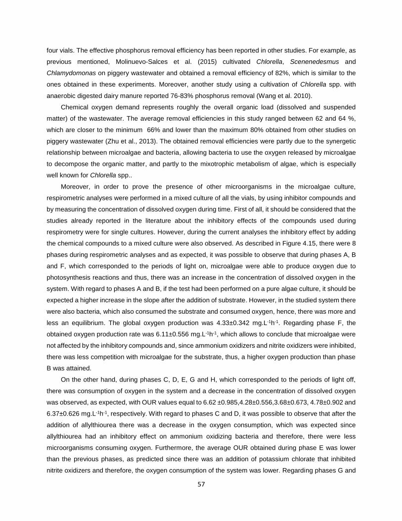
57
four vials. The effective phosphorus removal efficiency has been reported in other studies. For example, as
previous mentioned, Molinuevo-Salces et al. (2015) cultivated Chlorella, Scenenedesmus and
Chlamydomonas on piggery wastewater and obtained a removal efficiency of 82%, which is similar to the
ones obtained in these experiments. Moreover, another study using a cultivation of Chlorella spp. with
anaerobic digested dairy manure reported 76-83% phosphorus removal (Wang et al. 2010).
Chemical oxygen demand represents roughly the overall organic load (dissolved and suspended
matter) of the wastewater. The average removal efficiencies in this study ranged between 62 and 64 %,
which are closer to the minimum 66% and lower than the maximum 80% obtained from other studies on
piggery wastewater (Zhu et al., 2013). The obtained removal efficiencies were partly due to the synergetic
relationship between microalgae and bacteria, allowing bacteria to use the oxygen released by microalgae
to decompose the organic matter, and partly to the mixotrophic metabolism of algae, which is especially
well known for Chlorella spp..
Moreover, in order to prove the presence of other microorganisms in the microalgae culture,
respirometric analyses were performed in a mixed culture of all the vials, by using inhibitor compounds and
by measuring the concentration of dissolved oxygen during time. First of all, it should be considered that the
studies already reported in the literature about the inhibitory effects of the compounds used during
respirometry were for single cultures. However, during the current analyses the inhibitory effect by adding
the chemical compounds to a mixed culture were also observed. As described in Figure 4.15, there were 8
phases during respirometric analyses and as expected, it was possible to observe that during phases A, B
and F, which corresponded to the periods of light on, microalgae were able to produce oxygen due to
photosynthesis reactions and thus, there was an increase in the concentration of dissolved oxygen in the
system. With regard to phases A and B, if the test had been performed on a pure algae culture, it should be
expected a higher increase in the slope after the addition of substrate. However, in the studied system there
were also bacteria, which also consumed the substrate and consumed oxygen, hence, there was more and
less an equilibrium. The global oxygen production was 4.33±0.342 mg.L-1h-1. Regarding phase F, the
obtained oxygen production rate was 6.11±0.556 mg.L-1h-1, which allows to conclude that microalgae were
not affected by the inhibitory compounds and, since ammonium oxidizers and nitrite oxidizers were inhibited,
there was less competition with microalgae for the substrate, thus, a higher oxygen production than phase
B was attained.
On the other hand, during phases C, D, E, G and H, which corresponded to the periods of light off,
there was consumption of oxygen in the system and a decrease in the concentration of dissolved oxygen
was observed, as expected, with OUR values equal to 6.62 ±0.985,4.28±0.556,3.68±0.673, 4.78±0.902 and
6.37±0.626 mg.L-1h-1, respectively. With regard to phases C and D, it was possible to observe that after the
addition of allylthiourea there was a decrease in the oxygen consumption, which was expected since
allylthiourea had an inhibitory effect on ammonium oxidizing bacteria and therefore, there were less
microorganisms consuming oxygen. Furthermore, the average OUR obtained during phase E was lower
than the previous phases, as predicted since there was an addition of potassium chlorate that inhibited
nitrite oxidizers and therefore, the oxygen consumption of the system was lower. Regarding phases G and
58
H, as expected, there was an increase in the OUR after the addition of sodium acetate since it activated
heterotrophic organisms by working as a substrate and therefore, there was more consumption of oxygen.
Finally, another target of this study was to evaluate the suitability of the mixed microalgae culture used
for the piggery wastewater treatment as a substrate for biogas production by anaerobic digestion. Literature
(Yen & Brune, 2007) reports that the methane production by a mixed culture of Chlorella vulgaris and
Scenedesmus sp. is characterized by an inverse exponential curve, which is in agreement with the results
obtained (Figure 4.16) in the present study, where it was possible to observe a rapid methane production
increase during the first days, an intermediate phase in which biomethane production rate decreased and a
plateau phase after the 10th day of degradability. This inverse exponential curve can be explained by the
fact that the BMP tests were performed in batch conditions and, as time went by, the amount of substrate
decreased as well as the biomethane production rate.
In general, BMP values for microalgae found in the literature are diverse and usually ranged between
153 and 600 mLCH4.g-1 VS (Ward et al. 2014). Hence, it should be pointed out that methane production is
strongly dependent on the species and it has been observed (Mussgnug et al. 2010) that microalgae without
cell wall as Dunaliella salina or with protein-based membranes, such as Chlamydomonas reinhardtii,
Arthrospira platensis and Euglena gracilis, present a higher BMP values, between 481 and 587 mLCH4.g-
1VS, than microalgae species with a cell wall containing cellulose or hemicellulose as Scenedesmus
obliquus and Chlorella kessleri, which present BMP values comprised between 287-335 mLCH4.g-1 VS.
Therefore, it is possible to conclude that the cell wall degradability is strongly correlated with the quantity of
methane produced and sometimes pre-treatments should be considered to degrade the cell wall prior to
digestion. With regard to this experiment, microalgae were found to have an interesting methane production
potential and similar biomethane values were obtained for algae C and D, showing the good repeatability
of the test. The obtained data between 264.3 mLCH4.g-1 VS and 270.4 mLCH4.g-1 VS was comprised in the
usual range reported in the literature. Also, it was similar to the previous mentioned values for Scenedesmus
obliquus and Chlorella kessleri. Furthermore, the methane conversion during a study with a mixed culture
of Chlorella spp. and Scenedesmus spp. reached 143 mLCH4.g-1 VS (Yen & Brune, 2007), which is lower
than the results of the present study. In addition, the anaerobic digestion of piggery manure from Corte
Grand plant reached a BMP value of 150 mLCH4. g-1 VS (Marazzi et al. 2015), which is also much lower
than the BMP values obtained during this study. Therefore, the obtained values confirm that microalgae
biomass cultivated in nutrient-rich streams, such as piggery wastewater, is a feasible option for biogas
production.
59
6 Conclusions Agricultural wastewater is one of the most relevant contributors to environmental pollution due to its
high concentration of nutrients, such as nitrogen and phosphorus, as well as its high organic load. For years,
the traditional method to treat piggery wastewater was using it as land fertilizer, but the nitrogen in piggery
wastewater cannot be completely uptaken by crops due to the unbalanced N/P ratio and consequently, the
accumulation of nutrients in the soil can contaminate the receiving waters. Therefore, it is important to
investigate and to find the most efficient and environmentally friendly treatment method for piggery
wastewater.
The present study was devoted to evaluate the capacity of a mixed culture of Chlorella spp. and
Scenedesmus spp. to grow on a piggery wastewater (pre-treated with a flotation process) as well as their
bioremediation capacity to remove nutrients, such as nitrogen and phosphorus, and the culture suitability
for energy production.
The results from this study proved that these green microalgae were able to efficiently grow on the high
organic load medium, which is in agreement with previous studies that reported that Scenedesmus spp. and
Chlorella spp. are within the top 10 more resistance species. Moreover, these species also seemed to adapt
and recover from some drastic biomass decreases, which is an important aspect to take into account in a
WWTP since the input conditions can easily vary.
Furthermore, the microalgae based system proved its ability to remove phosphorus, ammonium
nitrogen as well as COD and the obtained removal efficiencies were in agreement with the literature data.
Regarding the removal of N-NH4+, the average removal efficiencies were ranged between 85-92% and
different mechanisms were responsible for the removal of nitrogen (nitrification, biomass uptake and
ammonia stripping), being the biomass uptake the most important mechanism. In the case of phosphorus,
the average removal efficiency was ranged between 78-82 % and the considered removal mechanisms
were biomass uptake and phosphorus precipitation due to high pH levels. With regard to COD, the average
removal efficiency was ranged between 62-64% and these results enhance the synergetic relation between
microalgae and bacteria, since the removal of COD was partly attributed to the microorganisms that made
use of the oxygen produced by microalgae during photosynthesis to decompose the organic matter present
in the wastewater and also, partly to the mixotrophic metabolism of microalgae.
Besides the removal of COD, the presence of other microorganisms was also proved by respirometric
analyses, which consisted in using inhibitors of ammonium oxidizers and nitrite oxidizers and measuring the
dissolved oxygen during time. Moreover, the used inhibitors proved to have the desired effect, since after
the addition of these compounds, it was observed a decrease in the oxygen consumption.
Finally, the other aim of this work was to investigate the feasibility of anaerobic digestion for biogas
production from the mixed culture of Chlorella spp. and Scenedesmus spp. used in the piggery wastewater
treatment. The rapid economic growth has led to high-energy consumption around the world and
60
consequently to the increase of environmental pollution. Biogas is an alternative energy source that can
overcome these concerns and microalgae are one interesting substrate for biomethane production due to
their high growth rate, high biomass yields and to their capacity to grow on wastewaters. The obtained
biomethane production was ranged between 264.3 and 270.4 mLCH4.g-1 VS, which is in agreement with
the literature data and is much higher than the BMP values obtained from the anaerobic digestion of piggery
manure from Corte Grande plant. Hence, the obtained values confirmed that microalgae biomass cultivated
in nutrients-rich streams, such as piggery wastewater, is a feasible option for biogas production.
Considering an appropriate process evaluation and design, the hypothesis of using algal-based
treatment as the first step of biological treatment of piggery wastewater could be considered. In that case,
algae biomass could be digested and the liquid phase of digestate could be recirculated upflow to be treated
by algae/bacteria consortium along with the pre-treated piggery wastewater.
61
7 Future Perspectives Based on the work done and the results obtained, the following recommendations can be suggested:
Studying the effects of N/P ratio on the mixed culture to investigate if it affects microalgae
growth and the nutrient removal efficiency;
Investigating with detail mixotrophic microalgae since they are poorly studied and they can
take advantage of both organic and inorganic substrates to obtain higher biomass production,
which is very interesting in the integration of microalgae cultivation with wastewater treatment
processes where the wastewater is usually turbid and the light cannot penetrate into its core
body. Moreover, studying these mixotrophic conditions to improve the removal of COD;
Improving the nitrogen biomass uptake mechanism, for example, by a tight control of the pH
values, which will decrease the ammonia volatilization;
Investigating the nitrification process in order to understand
the reasons for its discontinuity and for the eventual accumulation of
nitrites and its influence on algae growth. In fact, competition
for CO2 could take place and a certain lag is likely to be needed by
algae population grown on ammonium nitrogen to shift towards the uptake
of nitrate nitrogen.
Investigating possible pre-treatments for microalgae before BMP tests.
62
8 References
Abdel-Raouf, N., Al-Homaidan, A.A. & Ibraheem, I.B.M., 2012. Microalgae and wastewater
treatment. Saudi Journal of Biological Sciences, 19(3), pp.257–275. Available at:
http://dx.doi.org/10.1016/j.sjbs.2012.04.005.
Ahlenius, H., 2010. Ratio of wastewater treatment. Available at:
http://www.grida.no/graphicslib/detail/ratio-of-wastewater-treatment_9d38.
Al-Qasmi, M. et al., 2012. A Review of Effect of Light on Microalgae Growth. Proceedings of the
World Congress on Engineering, I, pp.8–10.
Arthur, R., Baidoo, M.F. & Antwi, E., 2011. Biogas as a potential renewable energy source: A
Ghanaian case study. Renewable Energy, 36(5), pp.1510–1516. Available at:
http://dx.doi.org/10.1016/j.renene.2010.11.012.
Azov, Y. & Goldman, J.C., 1982. Free ammonia inhibition of algal photosynthesis in intensive
cultures. Applied and environmental microbiology, 43(4), pp.735–739.
Bernet, N. & Béline, F., 2009. Challenges and innovations on biological treatment of livestock
effluents. Bioresource Technology, 100(22), pp.5431–5436. Available at:
http://dx.doi.org/10.1016/j.biortech.2009.02.003.
Boelee, N.C. et al., 2011. Nitrogen and phosphorus removal from municipal wastewater effluent
using microalgal biofilms. Water Research, 45(18), pp.5925–5933. Available at:
http://dx.doi.org/10.1016/j.watres.2011.08.044.
Borowitzka, M.A., Beardall, J. & Ravens, J.A., 2016. The Physiology of Microalgae,
Boursier, H., Béline, F. & Paul, E., 2005. Piggery wastewater characterisation for biological nitrogen
removal process design. Bioresource Technology, 96(3), pp.351–358.
Bradley, A.L., 2015. Materials Management and the Circular Economy. Available at:
https://nerc.org/news-and-updates/blog/nerc-blog/2015/05/12/materials-management-and-the-
circular-economy.
Brennan, L. & Owende, P., 2010. Biofuels from microalgae-A review of technologies for production,
processing, and extractions of biofuels and co-products. Renewable and Sustainable Energy
Reviews, 14(2), pp.557–577.
Brown, N. & Shilton, A., 2014. Luxury uptake of phosphorus by microalgae in waste stabilisation
ponds: Current understanding and future direction. Reviews in Environmental Science and
Biotechnology, 13(3), pp.321–328.
Bumbak, F. et al., 2011. Best practices in heterotrophic high-cell-density microalgal processes:
Achievements, potential and possible limitations. Applied Microbiology and Biotechnology, 91(1),
63
pp.31–46.
Bux, F., 2013. Biotechnological Applications of Microalgae:Biodiesel and Value-Added Products,
Cai, T., Park, S.Y. & Li, Y., 2013. Nutrient recovery from wastewater streams by microalgae: Status
and prospects. Renewable and Sustainable Energy Reviews, 19, pp.360–369. Available at:
http://dx.doi.org/10.1016/j.rser.2012.11.030.
Cao, G. & Orrù, R., 2014. Current Environmental issues and challenges,
Cellis, J.E., 2006. Cell biology: A laboratory handbook,
Chen, C.Y. et al., 2013. Microalgae-based carbohydrates for biofuel production. Biochemical
Engineering Journal, 78(August 2016), pp.1–10.
Chen, C.Y. & Durbin, E.G., 1994. Effects of pH on the growth and carbon uptake of marine
phytoplankton. Marine Ecology Progress Series, 109(1992), pp.83–94.
Chen, G.Q. & Chen, F., 2006. Growing phototrophic cells without light. Biotechnology Letters, 28(9),
pp.607–616.
Chen, W., Tong, H. & Liu, H., 2012. Effects of nitrate on nitrite toxicity to Microcystis aeruginosa.
Marine Pollution Bulletin, 64(6), pp.1106–1111. Available at:
http://dx.doi.org/10.1016/j.marpolbul.2012.04.006.
Chen, W., Zhang, Q. & Dai, S., 2009. Effects of nitrate on intracellular nitrite and growth of
Microcystis aeruginosa. Journal of Applied Phycology, 21(6), pp.701–706.
Chisti, Y., 2007. Biodiesel from microalgae. Trends in Biotechnology, 26(3), pp.295–304. Available
at: http://dx.doi.org/10.1016/j.biotechadv.2007.02.001.
Chisti, Y. et al., 2014. Biofuels from algae,
Chisti, Y., 2010. Fuels from microalgae. Biofuels, 1(2), pp.233–235.
Chiu, S.Y. et al., 2011. Microalgal biomass production and on-site bioremediation of carbon dioxide,
nitrogen oxide and sulfur dioxide from flue gas using Chlorella sp. cultures. Bioresource
Technology, 102(19), pp.9135–9142. Available at: http://dx.doi.org/10.1016/j.biortech.2011.06.091.
Choi, H.J. & Lee, S.M., 2015. Effect of the N/P ratio on biomass productivity and nutrient removal
from municipal wastewater. Bioprocess and Biosystems Engineering, 38(4), pp.761–766.
Chu, H.Q. et al., 2015. Continuous cultivation of Chlorella pyrenoidosa using anaerobic digested
starch processing wastewater in the outdoors. Bioresource Technology, 185, pp.40–48. Available
at: http://dx.doi.org/10.1016/j.biortech.2015.02.030.
Chynoweth, D.P.., Wilkie, a. C.. & Owens, J.M., 1999. Anaerobic processing of piggery waste: a
review. Asian-Australasian Association of Animal Societies, 12(4), pp.607–628.
Collet, P. et al., 2014. Biodiesel from microalgae - Life cycle assessment and recommendations for
potential improvements. Renewable Energy, 71, pp.525–533.
Collos, Y. & Harrison, P.J., 2014. Acclimation and toxicity of high ammonium concentrations to
unicellular algae. Marine Pollution Bulletin, 80(1–2), pp.8–23. Available at:
http://dx.doi.org/10.1016/j.marpolbul.2014.01.006.
64
Costa, J.A.V. & de Morais, M.G., 2014. Biofuels from algae,
Costa, R.H.R. et al., 2006. Algae biomass evaluation in aerated facultative maturation ponds for
piggery waste treatment and. , (1995).
Dahmani, S. et al., 2016. Cultivation of Chlorella pyrenoidosa in outdoor open raceway pond using
domestic wastewater as medium in arid desert region. Bioresource Technology, 219, pp.749–752.
Available at: http://dx.doi.org/10.1016/j.biortech.2016.08.019.
De-Bashan, L.E. et al., 2008. Role of glutamate dehydrogenase and glutamine synthetase in
Chlorella vulgaris during assimilation of ammonium when jointly immobilized with the microalgae-
growth-promoting bacterium Azospirillum brasilense. Journal of Phycology, 44(5), pp.1188–1196.
Dyhrman, S.T. & Ruttenberg, K.C., 2006. Presence and regulation of alkaline phosphatase activity
in eukaryotic phytoplankton from the coastal ocean: Implications for dissolved organic phosphorus
remineralization. Limnology and Oceanography, 51(3), pp.1381–1390.
de Fernicola, N.G. & de Azevedo, F.A., 1981. Metemoglobinemia e nitrato nas águas. Revista de
Saude Publica, 15(2), pp.242–248.
Fewtrell, L., 2004. Drinking-water nitrate, methemoglobinemia, and global burden of disease: A
discussion. Environmental Health Perspectives, 112(14), pp.1371–1374.
Flynn, K.J. & Butler, I., 1986. Nitrogen sources for the growth of marine microalgae : role of
dissolved free amino acids. Marine Ecology Progress Series, 34(1958), pp.281–304.
Gao, F. et al., 2016. Continuous microalgae cultivation in aquaculture wastewater by a membrane
photobioreactor for biomass production and nutrients removal. Ecological Engineering, 92, pp.55–
61. Available at: http://www.sciencedirect.com/science/article/pii/S0925857416302014.
Geider, R. & Roche, J. La, 2011. Redfield revisited: variability of C:N:P in marine microalgae and
its biochemical basis Redfield revisited: variability of C:N:P in marine microalgae and its biochemical
basis. European Journal of Phycology, 37(September 2012), pp.37–41.
Geographer, M.S. & Irvine, K.N., 2002. Turbidity , Suspended Solids , and Bacteria Relationships
in the Buffalo River Watershed. , pp.42–51.
Ginestet, P. et al., 1998. Estimation of nitrifying bacterial activities by measuring oxygen uptake in
the presence of the metabolic inhibitors allylthiourea and azide. Applied and Environmental
Microbiology, 64(6), pp.2266–2268.
Girard, M. et al., 2009. A review of the environmental pollution originating from the piggery industry
and of the available mitigation technologies: towards the simultaneous biofiltration of swine slurry
and methaneThis article is one of a selection of papers published in this Sp. Canadian Journal of
Civil Engineering, 36(12), pp.1946–1957.
Godos, I. de et al., 2010. A comparative evaluation of microalgae for the degradation of piggery
wastewater under photosynthetic oxygenation. Bioresource Technology, 101(14), pp.5150–5158.
Available at: http://dx.doi.org/10.1016/j.biortech.2010.02.010.
Godos, I. de et al., 2009. Long-term operation of high rate algal ponds for the bioremediation of
65
piggery wastewaters at high loading rates. Bioresource Technology, 100(19), pp.4332–4339.
Available at: http://dx.doi.org/10.1016/j.biortech.2009.04.016.
Golueke, C.G., Oswald, W.J. & Gotaas, H.B., 1957. Anaerobic digestion of Algae. Applied
microbiology, 5, pp.47–55.
González-Fernández, C. et al., 2016. Impact of temperature and photoperiod on anaerobic
biodegradability of microalgae grown in urban wastewater. International Biodeterioration and
Biodegradation, 106, pp.16–23.
Griffiths, M.J. et al., 2011. Interference by pigment in the estimation of microalgal biomass
concentration by optical density. Journal of Microbiological Methods, 85(2), pp.119–123.
Heredia-Arroyo, T. et al., 2011. Mixotrophic cultivation of Chlorella vulgaris and its potential
application for the oil accumulation from non-sugar materials. Biomass and Bioenergy, 35(5),
pp.2245–2253.
Herrero, M., Cifuentes, A. & Iba??ez, E., 2006. Sub- and supercritical fluid extraction of functional
ingredients from different natural sources: Plants, food-by-products, algae and microalgae - A
review. Food Chemistry, 98(1), pp.136–148.
Hjorth, M. et al., 2010. Solid-liquid separation of animal slurry in theory and practice. A review.
Agronomy for Sustainable Development, 30(1), pp.153–180. Available at:
http://dx.doi.org/10.1051/agro/2009010.
Hodaifa, G., Mart??nez, M.E. & S??nchez, S., 2009. Influence of pH on the culture of Scenedesmus
obliquus in olive-mill wastewater. Biotechnology and Bioprocess Engineering, 14(6), pp.854–860.
Hook, M. & Tang, X., 2013. Depletion of fossil fuels and anthropogenic climate change-A review.
Energy Policy, 52, pp.797–809.
Hynes, R.K. & Knowles, R., 1983. Inhibition of chemoautrophic nitrification by sodium chlorate and
sodium chlorite: A reexamination. Applied and Environmental Microbiology, 45(4), pp.1178–1182.
Iregbu, G.U. et al., 2014. Environmental concerns of pig waste production and its potentials as
biofuel source To cite this article. , 1(3), pp.17–24.
John, D.M., Whitton, B.A. & Brook, A.J., 2002. The Freshwater Algal Flora of the British Isles: An
Identification guide to freshwater and terrestrial algae, Volume 1,
de la Noüe, J., Laliberté, G. & Proulx, D., 1992. Algae and waste water. Journal of Applied
Phycology, 4(3), pp.247–254.
Lara-Gil, J.A., Álvarez, M.M. & Pacheco, A., 2014. Toxicity of flue gas components from cement
plants in microalgae CO2 mitigation systems. Journal of Applied Phycology, 26(1), pp.357–368.
Lara-Gil, J.A., Senés-Guerrero, C. & Pacheco, A., 2016. Cement flue gas as a potential source of
nutrients during CO2 mitigation by microalgae. Algal Research, 17, pp.285–292. Available at:
http://linkinghub.elsevier.com/retrieve/pii/S2211926416301734.
Li, Y. et al., 2008. Biocatalysts and bioreactor design. Biotechnol, 1(3), pp.815–820. Available at:
http://dx.doi.org/10.1002/047167849X.bio005.
66
Lim, S.J. et al., 2016. Enhanced treatment of swine wastewater by electron beam irradiation and
ion-exchange biological reactor. Separation and Purification Technology, 157, pp.72–79. Available
at: http://dx.doi.org/10.1016/j.seppur.2015.03.021.
Lowrey, J., Brooks, M.S. & McGinn, P.J., 2015. Heterotrophic and mixotrophic cultivation of
microalgae for biodiesel production in agricultural wastewaters and associated challenges???a
critical review. Journal of Applied Phycology, 27(4), pp.1485–1498.
Manivanan, R., 2008. Water Quality Modeling: Rivers, Streams and Estuaries,
Marazzi, F. et al., 2015. Microalgal based treatment of digested agro wastes - lab and pilot-scale
experiments,
Markou, G., Vandamme, D. & Muylaert, K., 2014. Microalgal and cyanobacterial cultivation: The
supply of nutrients. Water Research, 65, pp.186–202. Available at:
http://dx.doi.org/10.1016/j.watres.2014.07.025.
Masse, D. et al., 1997. Potential for the Psychrophilic Anaerobic Treatment of Swine Manure Using
a Sequencing Batch Reactor. Canadian Agricultural Engineering, 39(1), pp.25–33.
Mata, T.M., Martins, A. a. & Caetano, N.S., 2010. Microalgae for biodiesel production and other
applications: A review. Renewable and Sustainable Energy Reviews, 14(1), pp.217–232.
MAY, W.A., 1997. Effects of temperature and {pH} on the growth kinetics of unialga {Chlorella}
vulgaris cultures containing bacteria. Water Environment Research, 69(1), pp.64–72.
Means, E., 2004. Water and Wastewater Industry Energy Efficiency: A Research Roadmap. Awwa
Research Foundation, pp.1–110.
Mezzanotte, V., Ficara, E. & Marazzi, F., 2015. LE MICROALGHE E LA LORO INTEGRAZIONE
NEGLI IMPIANTI DI DIGESTIONE ANAEROBICA,
Mo, W.W. & Zhang, Q., 2012. Can municipal wastewater treatment systems be carbon neutral?
Journal of Environmental Management, 112, pp.360–367.
Molinuevo-Salces, B. et al., 2015. From piggery wastewater nutrients to biogas: Microalgae
biomass revalorization through anaerobic digestion. Renewable Energy, 96, pp.1103–1110.
Monlau, F. et al., 2015. New opportunities for agricultural digestate valorization: current situation
and perspectives. Energy Environ. Sci., pp.2600–2621. Available at:
http://xlink.rsc.org/?DOI=C5EE01633A.
de Morais, M.G. & Costa, J.A. V, 2007. Isolation and selection of microalgae from coal fired
thermoelectric power plant for biofixation of carbon dioxide. Energy Conversion and Management,
48(7), pp.2169–2173.
Morales-Sanchez, D. et al., 2014. Heterotrophic growth of microalgae: metabolic aspects. World
Journal of Microbiology and Biotechnology, pp.1–9.
Morgan, M., 2005. Images of desmids from the genus Scenedesmus. Available at:
http://www.microscopy-uk.org.uk/mag/artoct05/mmdesmid
Muñoz, R. & Guieysse, B., 2006. Algal-bacterial processes for the treatment of hazardous
67
contaminants: A review. Water Research, 40(15), pp.2799–2815.
Mussgnug, J.H. et al., 2010. Microalgae as substrates for fermentative biogas production in a
combined biorefinery concept. Journal of Biotechnology, 150(1), pp.51–56. Available at:
http://dx.doi.org/10.1016/j.jbiotec.2010.07.030.
Nollet, L.M.L. & Gelder, L.S.P. De, 2014. Handbook of Water Analysis, Third Edition,
Obaja, D. et al., 2003. Nitrification, denitrification and biological phosphorus removal in piggery
wastewater using a sequencing batch reactor. Bioresource Technology, 87(1), pp.103–111.
Olaizola, M., 2003. Commercial development of microalgal biotechnology: From the test tube to the
marketplace. Biomolecular Engineering, 20(4–6), pp.459–466.
Olguín, E.J. et al., 2003. Annual productivity of Spirulina (Arthrospira) and nutrient removal in a pig
wastewater recycling process under tropical conditions. Journal of Applied Phycology, 15(2–3),
pp.249–257.
Ortiz-Ospina, E. & Roser, M., 2016. World Population growth. Available at:
https://ourworldindata.org/world-population-growth/.
Pandey, S., 2006. Water pollution and health. Kathmandu University medical journal (KUMJ), 4(1),
pp.128–34. Available at: http://www.ncbi.nlm.nih.gov/pubmed/24838129.
Park, J.B.K., Craggs, R.J. & Shilton, A.N., 2011. Wastewater treatment high rate algal ponds for
biofuel production. Bioresource Technology, 102(1), pp.35–42. Available at:
http://dx.doi.org/10.1016/j.biortech.2010.06.158.
Park, S. & Li, Y., 2012. Evaluation of methane production and macronutrient degradation in the
anaerobic co-digestion of algae biomass residue and lipid waste. Bioresource Technology, 111,
pp.42–48. Available at: http://dx.doi.org/10.1016/j.biortech.2012.01.160.
Parmar, A. et al., 2011. Cyanobacteria and microalgae: A positive prospect for biofuels. Bioresource
Technology, 102(22), pp.10163–10172. Available at:
http://dx.doi.org/10.1016/j.biortech.2011.08.030.
Passos, F. et al., 2013. Biogas production from microalgae grown in wastewater: Effect of
microwave pretreatment. Applied Energy, 108, pp.168–175. Available at:
http://dx.doi.org/10.1016/j.apenergy.2013.02.042.
Perales-Vela, H.V., Peña-Castro, J.M. & Cañizares-Villanueva, R.O., 2006. Heavy metal
detoxification in eukaryotic microalgae. Chemosphere, 64(1), pp.1–10.
Perez-Garcia, O. et al., 2011. Heterotrophic cultures of microalgae: Metabolism and potential
products. Water Research, 45(1), pp.11–36. Available at:
http://dx.doi.org/10.1016/j.watres.2010.08.037.
De Philippis, R., Colica, G. & Micheletti, E., 2011. Exopolysaccharide-producing cyanobacteria in
heavy metal removal from water: Molecular basis and practical applicability of the biosorption
process. Applied Microbiology and Biotechnology, 92(4), pp.697–708.
Pires, J.C.M. et al., 2012. Carbon dioxide capture from flue gases using microalgae: Engineering
68
aspects and biorefinery concept. Renewable and Sustainable Energy Reviews, 16(5), pp.3043–
3053. Available at: http://dx.doi.org/10.1016/j.rser.2012.02.055.
Prescott, D.M., 1964. Methods in Cell Physiology,
Priyadarshani, I. & Rath, B., 2012. Commercial and industrial applications of micro algae – A review.
Journal of Algal Biomass Utilization, 3(4), pp.89–100.
Ra, C.S. et al., 2000. Biological Nutrient Removal With an Internal Organic Carbon Source in
Piggery Wastewater Treatment. , 34(3), pp.965–973.
Ras, M. et al., 2011. Experimental study on a coupled process of production and anaerobic
digestion of Chlorella vulgaris. Bioresource Technology, 102(1), pp.200–206. Available at:
http://dx.doi.org/10.1016/j.biortech.2010.06.146.
Ras, M., Steyer, J.P. & Bernard, O., 2013. Temperature effect on microalgae: A crucial factor for
outdoor production. Reviews in Environmental Science and Biotechnology, 12(2), pp.153–164.
Rasdi, N.W. & Qin, J.G., 2014. Effect of N:P ratio on growth and chemical composition of
Nannochloropsis oculata and Tisochrysis lutea. Journal of Applied Phycology, 27(6), pp.2221–
2230.
Raso, S. et al., 2011. Effect of oxygen concentration on the growth of Nannochloropsis sp. at low
light intensity. Journal of Applied Phycology, 24(4), pp.863–871. Available at:
http://www.pubmedcentral.nih.gov/articlerender.fcgi?artid=3392507&tool=pmcentrez&rendertype=
abstract.
Rawat, I., Gupta, S.K. & Bux, F., 2016. Microalgae applications in wastewater treatment. Algae
Biotechnology, Green Energy and Technology, (August), pp.249–268. Available at:
http://link.springer.com/10.1007/978-3-319-12334-9.
Rekacewicz, P., 2012. Freshwater stress 1995 and 2025. Available at:
http://www.grida.no/graphicslib/detail/freshwater-stress-1995-and-2025_6250.
Renuka, N. et al., 2015. Phycoremediation of wastewaters: a synergistic approach using microalgae
for bioremediation and biomass generation. International Journal of Environmental Science and
Technology, 12(4), pp.1443–1460.
Richmond, A., 2004. Handbook of Microalgal culture: Biotechnology and Applied Phycology,
Risgaard-Petersen, N. et al., 2004. Competition between ammonia-oxidizing bacteria and benthic
microalgae. Applied and Environmental Microbiology, 70(9), pp.5528–5537.
Roy, S. et al., 2011. Phytoplankton Pigments: Characterization, Chemotaxonomy and Applications
in Oceanography.,
Ruiz-Marin, A., Mendoza-Espinosa, L.G. & Stephenson, T., 2010. Growth and nutrient removal in
free and immobilized green algae in batch and semi-continuous cultures treating real wastewater.
Bioresource Technology, 101(1), pp.58–64. Available at:
http://dx.doi.org/10.1016/j.biortech.2009.02.076.
Ruiz-Martinez, A. et al., 2012. Microalgae cultivation in wastewater: Nutrient removal from
69
anaerobic membrane bioreactor effluent. Bioresource Technology, 126, pp.247–253. Available at:
http://dx.doi.org/10.1016/j.biortech.2012.09.022.
Salih, F.M., 2011. Microalgae Tolerance to High Concentrations of Carbon Dioxide: A Review.
Journal of Environmental Protection, 2(5), pp.648–654.
Santos-Ballardo, D.U. et al., 2016. Microalgae potential as a biogas source: current status,
restraints and future trends. Reviews in Environmental Science and Biotechnology, pp.1–22.
Sanz-Luque, E. et al., 2015. Understanding nitrate assimilation and its regulation in microalgae.
Frontiers in plant science, 6(October), p.899. Available at:
https://www.researchgate.net/publication/284029329_Understanding_nitrate_assimilation_and_its
_regulation_in_microalgae.
Se-Kwon, K., 2015. Handbook of Marine Microalgae:Biotechnology Advances,
Sialve, B., Bernet, N. & Bernard, O., 2009. Anaerobic digestion of microalgae as a necessary step
to make microalgal biodiesel sustainable. Biotechnology Advances, 27(1), pp.409–416. Available
at: http://dx.doi.org/10.1016/j.biotechadv.2009.03.001.
Sivakumar, K., Kumaresan, G. & Kesavamoorthy, K., 2016. I International Journal of Innovations in
Agricultural Sciences ( IJIAS ) Journal of In PRODUCTION OF BIODIESEL BY MICROALGAE AND
MACROALGAE FROM MANGROVES OF PICHAVARAM. , pp.51–56.
Škaloud, P., 2007. Image gallery of CAUP strains. Available at:
http://botany.natur.cuni.cz/algo/CAUP/H1955_Chlorella_vulgaris.htm.
Spolaore, P. et al., 2006. Commercial applications of microalgae. Journal of bioscience and
bioengineering, 101(2), pp.87–96. Available at:
http://www.sciencedirect.com/science/article/pii/S1389172306705497.
Tilley, D.F., 2011. Aerobic Wastewater Treatment Processes,
Tosta, A. & Mendonça, F., 2009. Technical analysis of the new brazilian concentration limits for
ammonia in effluents and bodies of water. Power, (27), pp.353–362.
Uggetti, E. et al., 2014. Anaerobic digestate as substrate for microalgae culture: The role of
ammonium concentration on the microalgae productivity. Bioresource Technology, 152, pp.437–
443. Available at: http://dx.doi.org/10.1016/j.biortech.2013.11.036.
Ugwu, C.U., Aoyagi, H. & Uchiyama, H., 2008. Photobioreactors for mass cultivation of algae.
Bioresource Technology, 99(10), pp.4021–4028.
Vergara-Fernández, A. et al., 2008. Evaluation of marine algae as a source of biogas in a two-stage
anaerobic reactor system. Biomass and Bioenergy, 32(4), pp.338–344.
Wang, B. et al., 2008. CO2 bio-mitigation using microalgae. Applied Microbiology and
Biotechnology, 79(5), pp.707–718.
Wang, L. et al., 2010. Anaerobic digested dairy manure as a nutrient supplement for cultivation of
oil-rich green microalgae Chlorella sp. Bioresource Technology, 101(8), pp.2623–2628. Available
at: http://dx.doi.org/10.1016/j.biortech.2009.10.062.
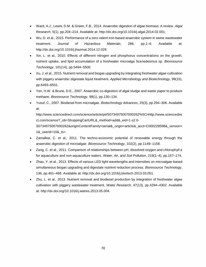
70
Ward, A.J., Lewis, D.M. & Green, F.B., 2014. Anaerobic digestion of algae biomass: A review. Algal
Research, 5(1), pp.204–214. Available at: http://dx.doi.org/10.1016/j.algal.2014.02.001.
Wu, D. et al., 2015. Performance of a zero valent iron-based anaerobic system in swine wastewater
treatment. Journal of Hazardous Materials, 286, pp.1–6. Available at:
http://dx.doi.org/10.1016/j.jhazmat.2014.12.029.
Xin, L. et al., 2010. Effects of different nitrogen and phosphorus concentrations on the growth,
nutrient uptake, and lipid accumulation of a freshwater microalga Scenedesmus sp. Bioresource
Technology, 101(14), pp.5494–5500.
Xu, J. et al., 2015. Nutrient removal and biogas upgrading by integrating freshwater algae cultivation
with piggery anaerobic digestate liquid treatment. Applied Microbiology and Biotechnology, 99(15),
pp.6493–6501.
Yen, H.W. & Brune, D.E., 2007. Anaerobic co-digestion of algal sludge and waste paper to produce
methane. Bioresource Technology, 98(1), pp.130–134.
Yusuf, C., 2007. Biodiesel from microalgae. Biotechnology Advances, 25(3), pp.294–306. Available
at:
http://www.sciencedirect.com/science/article/pii/S0734975007000262%5Cnhttp://www.sciencedire
ct.com/science?_ob=ShoppingCartURL&_method=add&_eid=1-s2.0-
S0734975007000262&originContentFamily=serial&_origin=article&_acct=C000228598&_version=
1&_userid=10&_ts=.
Zamalloa, C. et al., 2011. The techno-economic potential of renewable energy through the
anaerobic digestion of microalgae. Bioresource Technology, 102(2), pp.1149–1158.
Zang, C. et al., 2011. Comparison of relationships between pH, dissolved oxygen and chlorophyll a
for aquaculture and non-aquaculture waters. Water, Air, and Soil Pollution, 219(1–4), pp.157–174.
Zhao, Y. et al., 2013. Effects of various LED light wavelengths and intensities on microalgae-based
simultaneous biogas upgrading and digestate nutrient reduction process. Bioresource Technology,
136, pp.461–468. Available at: http://dx.doi.org/10.1016/j.biortech.2013.03.051.
Zhu, L. et al., 2013. Nutrient removal and biodiesel production by integration of freshwater algae
cultivation with piggery wastewater treatment. Water Research, 47(13), pp.4294–4302. Available
at: http://dx.doi.org/10.1016/j.watres.2013.05.004.
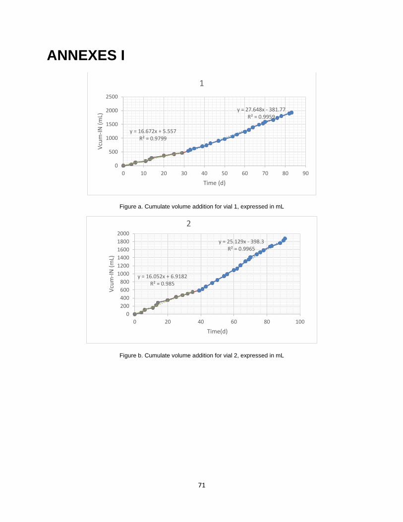
71
ANNEXES I
Figure a. Cumulate volume addition for vial 1, expressed in mL
Figure b. Cumulate volume addition for vial 2, expressed in mL
y = 16.672x + 5.557R² = 0.9799
y = 27.648x - 381.77R² = 0.9959
0
500
1000
1500
2000
2500
0 10 20 30 40 50 60 70 80 90
Vcu
m-I
N (
mL)
Time (d)
1
y = 16.052x + 6.9182R² = 0.985
y = 25.129x - 398.3R² = 0.9965
0
200
400
600
800
1000
1200
1400
1600
1800
2000
0 20 40 60 80 100
Vcu
m-I
N (
mL)
Time(d)
2
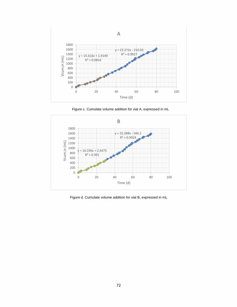
72
Figure c. Cumulate volume addition for vial A, expressed in mL
Figure d. Cumulate volume addition for vial B, expressed in mL
y = 15.616x + 1.9149R² = 0.9854
y = 23.272x - 210.03R² = 0.9927
0
200
400
600
800
1000
1200
1400
1600
1800
0 20 40 60 80 100
Vcu
m,in
(m
L)
Time (d)
A
y = 16.036x + 2.6475R² = 0.991
y = 22.288x - 166.1R² = 0.9918
0
200
400
600
800
1000
1200
1400
1600
1800
0 20 40 60 80 100
Vcu
m,in
(m
L)
Time (d)
B