i

Micro-Savings & Informal Insurance in Villages: A Field Experiment

on Indirect Effects of Financial Deepening on Safety Nets of the Poor

Jeffrey A. Flory Department of Agricultural and Resource Economics

University of Maryland 2200 Symons Hall

College Park, MD 20742 jflory@arec.umd.edu

Draft July 18, 2011

Selected Paper prepared for presentation at the Agricultural & Applied Economics Association’s 2011 AAEA & NAREA Joint Annual Meeting, Pittsburgh, Pennsylvania,

July 24-26, 2011

Copyright 2011 by Jeffrey A. Flory. All rights reserved. Readers may make verbatim copies of this document for non-commercial purposes by any means, provided that this copyright notice

appears on all such copies.

ii

Micro-Savings & Informal Insurance in Villages:

A Field Experiment on Indirect Effects of Financial Deepening on Safety Nets of the Poor

.

Jeffrey A. Flory1

July 18, 2011

Key words: Microfinance, formal savings, indirect effects, safety nets, poverty, food security JEL Codes: O17, O16, O12, I30, I38, I10

Abstract This paper exploits a unique micro dataset that uses a natural field experiment to identify indirect effects of formal savings access on de facto ineligibles residing in the same community. Despite widespread interest in microfinance as a poverty-reduction tool, the indirect effects on the very poor of expanding formal financial services remain largely unexplored. This study examines evidence from a large field experiment which helps fill this gap. It also contributes to an important emerging literature on the indirect impacts of policy interventions in developing countries, often (incompletely) evaluated solely on the basis of how they impact participants and beneficiaries. In developing regions, households vulnerable to extreme poverty often benefit from long-standing local safety nets based on cash gifts and other transfers from relatives and friends, which help them smooth consumption across food-deficits and household shocks. To date, little is known about how these pre-existing practices are affected as community members begin adopting newly available formal financial services, and there remains much unexplored in the interaction of formal financial markets with informal safety nets. This paper addresses that gap by examining how formal savings expansion affects inter-household wealth transfers, with a particular emphasis on receipts by the most vulnerable. Using a rich panel dataset from Central Malawi that includes over 2,000 households, I find that experimentally boosting local savings uptake in rural areas leads to a strong positive effect on assistance receipts by non service-users during peak periods of hunger. The difference is strongest among the most vulnerable households. That is, the entrance of formal savings appears to complement local informal support systems for the highly vulnerable through an indirect mechanism, channeling greater wealth to such households during periods of food-deficits. The positive impacts of formal savings expansion on non service-users suggests that formal savings may have substantially greater benefits than would be suggested by focusing exclusively on the impacts experienced by the service-users themselves.

1 University of Maryland, Department of Agricultural and Resource Economics, 2200 Symons Hall, College Park, MD 20742, jflory@arec.umd.edu.

1

I. Introduction

Interest in non-credit microfinance services has grown sharply in recent years among

development policy-makers and practitioners. There is great enthusiasm, for example, over

instruments such as crop-insurance for poor farmers, and several large aid organizations have

made it their mission to expand access to formal savings across the developing world. In the

earlier excitement over micro-credit, the potential welfare benefits of savings and insurance

services for the poor were given comparatively little attention. Now, as poverty-reduction policy

shifts its focus to include these other financial technologies in the push to extend access to capital

markets, there remain crucial gaps in our understanding of potential effects. Due perhaps to a

lack of suitable datasets, there is still little research on how the expansion of formal services will

interact with pre-existing practices in rural communities key to the welfare of many households,

and whether this will lead to differential outcomes among the poor.

Households across the developing world face frequent, and often severe, adverse income

and consumption shocks, particularly in rural settings. Communities excluded from formal

financial markets typically have vibrant, if imperfect, informal financial tools and safety-net

systems to help household smooth consumption and prevent low outcomes during hard times. It

is unclear a priori how these pre-existing systems will be affected by the introduction of market-

based instruments, and whether certain populations will be affected differently than others by the

changes that ensue. This amplifies the uncertainty over the impacts that financial deepening is

likely to have in rural areas of developing economies. Even if service-users themselves are

positively impacted by the new formal financial technologies they adopt (a hypothesis which

itself has been challenged), introducing new financial service options could still lead to mixed

results overall.

New services may benefit comparatively wealthy users, yet result in dire short-term and

long-term outcomes for very poor non-users. For example, if the latter suddenly lose access to

relatives’ cash-resources for emergency consumption-support, they may need to pull children

from school, forego medical treatment, or reduce food-intake. Alternative scenarios, however,

could result in benefits to both groups – for example, if access to formal services enhance the

management and accumulation of wealth which may be shared with any dependent households.

Large-scale introduction of formal savings services in rural areas of developing countries

is thus likely to interact with indigenous institutions which have already evolved to fulfill

2

important economic roles in villages. The interaction could result in unintended consequences

for non-users, which may be either negative or positive, and there remains scant evidence to

serve as a guide. To date, what little work has been done on micro-savings quite naturally tends

to focus on the individual who is taking up the new savings technology, or the new user’s

household. This handful of studies concentrate on understanding the direct outcomes on users of

things like commitment devices and new wealth management tools, and the mechanisms driving

these outcomes. Few studies have considered the broader economic and institutional contexts in

which these new product take-up decisions are being made, and no one seems to have explicitly

considered spillover effects on the non-using population.

Townsend (1995) makes an intriguing observation about risk-bearing capacities among

the villages he studies in northern Thailand. The village most integrated into outside markets had

a marked paucity of internal informal credit and insurance mechanisms, and more pronounced

negative shocks to consumption for households suffering a severe illness. This suggests that

deeper penetration of formal financial markets into villages could in fact weaken local risk-

bearing systems and social safety nets, a hypothesis echoed by Besley (1995) and Morduch

(1999).

Despite academic and policy interest in existing insurance arrangements for the poor in

villages and the ameliorative potential of financial markets in consumption-smoothing, there are

few serious studies on the interaction of the two. Perhaps this is due to a lack of datasets suitable

for examining the relationship of formal and informal institutions. Two exceptions are Ligon,

Thomas, and Worrall (2000), and Foster and Rosenzweig (2000). The former, a purely

theoretical contribution, models the introduction of an enhanced savings technology in the

presence of informal mutual insurance contracts. The latter paper models the simultaneous

introduction of formal savings and formal credit in a similar setting. In addition, it includes a

short empirical analysis, but identification of effects relies on distance from banks as an

instrument, which is subject to important endogeneity concerns. Both studies conclude that the

introduction of formal services tend to weaken informal insurance arrangements that are based

on inter-household wealth flows. Importantly, both follow the dominant perspective in the

literature on informal insurance, assuming transfers are bidirectional, based on the promise of

future reciprocation and the notion of mutual insurance – an assumption which may not always

be valid.

3

The present study advances this nascent line of research by examining impacts of formal

services on local safety nets through a cleaner and more direct empirical strategy – the

importance of which is underscored by the fact that the results run counter to the suggestions

thus far deriving from less well-identified observations. First, the analysis here empirically

disentangles the effects of formal savings from that of credit. This is not only important for a

more complete academic or theoretical understanding of the interaction of formal and informal

systems. The reality that expanded formal savings access may precede access to formal credit by

extended periods underscores the policy relevance of distinguishing the effects of formal savings

from formal credit, as the effects of one may materialize well before access to the other is

introduced. Second, identification of causal effects in the present study rests on a more solid

foundation than the handful of empirical observations collected thus far. By relying on a

randomly assigned instrument, the analysis of impacts avoids many of the endogeneity concerns

that hinder the sparse collection of current evidence regarding the impacts of formal capital

markets on informal insurance. Together with a simple theoretical framework which allows for

the possibility of unidirectional transfer relationships, the findings from this cleaner empirical

approach suggest a broadening of the commonly accepted theoretical underpinnings of transfer-

based insurance arrangements may be in order.

This paper contributes to this thin literature along a few other dimensions which are at

least as important, and which have not yet been addressed. By examining effects among

households of varying levels of vulnerability to low welfare states, this paper facilitates an

understanding of heterogeneous impacts of financial deepening across subpopulations of key

policy relevance. In addition, by identifying those least able to take advantage of new financial

products, the empirical strategy pursued here enables an analysis of the channels of effects

(indirect versus direct). While identifying an indirect channel of effects is interesting from a

theoretical perspective, its policy relevance comes from the fact that it accounts for the practical

reality of wealth-constrained access to formal services as their geographical reach expands. By

focusing on impacts of financial services expansion on safety nets and outcomes of the poorest

of the poor – those typically least in a position to start using formal services – the paper centers

analysis of extension of formal capital markets on one of the most crucial populations for anti-

poverty policy.

4

This paper also contributes to an important emerging literature on the local indirect

effects of policy interventions in developing countries – a literature whose importance is

highlighted by the continued failure to consider program impacts in non-participants in most

impact assessments. A seminal study in this new thread of the project evaluation literature is that

by Angelucci and DeGiorgi (2009), who find strong impacts from the Mexican welfare program,

Progresa, on households that are not eligible to participate in the program. They show that the

presence of informal insurance networks and inter-household transfers lead to positive spillover

effects onto households that are not direct beneficiaries. This underscores the importance of

accounting for the fact that many village settings are characterized by a greater degree of inter-

household interactions than other settings, making it easier for program effects to extend beyond

participating households. However, the program evaluation literature is generally focused on

how participants and beneficiaries are impacted. Depending on how indirect effects impact the

non-treated, this can lead to important over-assessment or under-assessment of program effects,

and incomplete or inaccurate impact estimates. The results of this study shed light on the

importance of broader local effects of an additional type of intervention which has become

commonplace in the developing world – that of microfinance.

Contrary to suggestions inferred from the limited existing evidence, the introduction of

formal savings technologies in rural Malawi has a significant positive effect on inter-household

wealth flows. In particular, in communities where formal savings rates were experimentally

boosted, the proportion of households receiving cash-gifts from other households during the

hungry season is nearly 50% higher (about 21% versus 31%). When restricting to the most

vulnerable households, for whom the impact is most clearly identifiable as via an indirect

channel, the difference grows to 180% (about 10% versus 28%). Instrumental variables estimates

indicate that, for every one percentage-point increase in the proportion of households using

formal savings, the worst-off households experience a three percentage-point increase in the

probability of receiving a cash gift.

In addition, changes in loan receipts by the most vulnerable category of households

experienced an uptick in savings-encouraged communities very similar in scale to the effects

observed for cash gifts. Villages assigned to the formal savings encouragement exhibit increases

in the proportion of highly vulnerable non-saving households receiving loans from friends and

relatives by 14.4 to 22.4 percentage points.

5

These increases in assistance-receipts are also associated with significant welfare

impacts. Living in communities that received the saving encouragement caused two-year

improvements in at least three key welfare indicators among the worst-off. Households are 11.8

to 16.3 percent more likely to exit the worst food-security category to enter one of the three other

less severe categories. They also experience a 1.3 to 1.4 reduction in a continuous food-

insecurity score, representing a 10-12% improvement over baseline values for this food-security

indicator. In addition, the worst-off households living in savings-encouraged communities were

12 to 17.4 percent less likely to report any members of the household as recently unwell.

That the experience of rural households in Central Malawi is at odds with key

implications of the sparse existing theoretical work on this question suggests the need for

theoretical innovation. While this study is primarily empirical in scope, its novel empirical

findings should help provide an important basis for building an integrated theory on institutional

change as institutions of modern finance meet informal institutions with growing frequency. It is

my hope that the empirical insights furnished by this study will help with the future construction

of models which better accommodate the expanded set of empirical data this paper brings to this

thin literature.

The rest of the paper is organized as follows. The next section explains the centrality of

risk and uncertainty in village life, its often severe consequences, indigenous responses in

attempt to smooth consumption, and possible implications of microfinance. Section 3 develops a

simple theoretical framework for analyzing the effects of formal savings services penetration in

different contexts. In an attempt to broaden the theoretical approach that has dominated the

literature on informal insurance institutions, a simple innovation allows for transfers which are

unidirectional (“charitable gifts”) rather than bidirectional (“mutual insurance), as is commonly

assumed. The model illustrates how the entrance of superior savings technologies can lead to

different effects when transfers are of one type or the other. Section 4 describes the empirical

setting, the data, and identification strategy used to test the model’s predictions. Section 5 looks

at the effects of the information intervention on local rates of financial services use (which I call

the “IIT”). Section 6 examines the relationship between the information-instrument and receipts

of cash and in-kind gifts among the most vulnerable households. Section 7 uses an instrumental-

variables analysis to estimate the Indirect Treatment Effect (ITE). Section 8 repeats the IIT and

6

instrumental-variables analysis to obtain the ITE for welfare outcomes among the highly

vulnerable. Section 9 concludes and indicates directions for future investigation.

2. Responses to Risk, and Possible Implications of Microfinance Interventions

A rich literature documents the central problem of risk in rural settings of developing

countries. From Zimbabwe to India to China, several studies detail the exposure of village

communities to substantial fluctuations in consumption levels due to periodic swings in income

and the inherent uncertainty surrounding agricultural livelihoods. Especially among the poorest,

who are already consuming at low-levels, negative shocks to consumption can often lead to dire

welfare outcomes, many of them with long-lasting or permanent effects. Documented examples

include serious illness, lower education levels (Alderman et. al.; Jacoby et. al., Dercon et. al.),

physical stunting (Foster 1995; Alderman et al; Dercon et. al.), and death (Rose, …).2

Households are not without recourse, however, in the face of adverse income and

consumption shocks. In the absence of formal markets, a variety of methods have indigenously

arisen to meet the threats posed by uncertainty and protect individuals from dangerously low

consumption. Variously referred to as “hunger insurance”, local “social security”, “non-market

institutions”, and “informal insurance arrangements”, strategies for managing risk and coping

with adverse outcomes generally fall into one of two categories: individual-based approaches

pursued in isolation, or interdependent approaches which rely on relationships with others.

That these

negative impacts are generally most sharply felt among the poorest underscores the importance

of understanding how consumption insurance among the worst-off is affected through

microfinance projects and the process of financial deepening.

One of the most common responses risk in isolation is to sacrifice current consumption to

transfer wealth forward to help cover any future shortfalls. Many studies show that even the very

poor save out of windfall seasons in order to smooth consumption upward during hard times (e.g.

Paxson 1992), employing a wide variety of possible assets, ranging from grain storage and

livestock to jewelry and other durables (see, for example, Deaton 1992; Rosenzweig and Wolpin, 2For more on long-term effects of negative shocks, permanent impacts of low-consumption, and links between health outcomes and risk, see also Dercon 2005, Dercon and Hoddinott 2005, Hoddinott and Kinsey 2001, Jalan and Ravallion 2004, Beegle at. al. 2006, Karlan and Morduch (2009) p.57.

7

1993; Fafchamps et. al. 1998). As Besley (1995) notes, however, it is often difficult to find assets

that yield positive returns, due partly to transaction costs, and covariate supply and demand

shocks which may cause sharp depreciation. Fafchamps et. al. (1998) find that livestock sales in

Burkina Faso are able to make up for only 15-30% of income shortfalls. In addition, as Giles and

Yoo (2007) point out, holding savings as a hedge against potential near-term income shortfalls

may prevent it from being more productively invested elsewhere.

Another strategy households may pursue in isolation is adjusting production and income-

generating decisions so as to dampen income volatility. While reducing variation in realized

income (and, more to the point, raising lower bounds for expected income ranges), this often

unfortunately lowers efficiency, reduces profits, and diminishes total household incomes over the

long-run. Morduch (1995) reviews several examples of this practice of “income-smoothing”.

Results from Antle (1987) and Bliss and Stern (1982) show input levels which lower variation in

net income, but which reduce expected profits. Walker and Ryan (1990) and Bliss and Stern

(1982) show households may delay farm investments to await more accurate weather

predictions. While this allows them to cut losses when they know weather will be poor, waiting

substantially reduces total expected yields.3 Morduch (1990) also finds that vulnerability of

consumption to shocks is linked to use of lower-risk, but lower-yielding, crop-varieties.4

The negative effects that income-smoothing can have on total incomes suggests

avoidance of this method by those with adequate alternative risk-coping options, often the

wealthier households. Binswanger and Rosenzweig (1993) show that the least well-off are most

likely to shift production toward safer, but less profitable, modes of production in the presence of

income volatility, leading to large income losses.

Spatial

diversification of income sources is another common strategy. Townsend (1995b) discusses the

possible gains from local crop fragmentation; Giles (2006) shows that households in rural China

use local off-farm labor markets as well as remittances from household members working in

more distant cities to reduce exposure of consumption to uncertainties of agricultural production.

5

3 Bliss and Stern (1982) estimate that delaying production by two weeks can reduce yields by 20% , in the village they study in northern India.

Changes in the availability of consumption-

4 Anecdotal evidence and information gathered from qualitative interviews in Central Malawi also suggests that, while farmers know that genetically modified maize may result in significantly higher yields, their concern that it has a higher risk of spoilage prevents them from using it. 5 They estimate that a standard deviation increase in rainfall timing variation has a negligible impact on production and profitability of the richest farmers, as they have adequate alternative risk-coping mechanisms, but lowers incomes among the bottom quartile by 35%.

8

insurance alternatives may therefore have disproportionately large impacts on the worst-off, once

again highlighting the importance of understanding how financial deepening affects consumption

insurance among the poorest.

Addressing short-falls in income through assistance from other households is also

common, and a rich literature documents an array of methods through which members of rural

communities help each other in times of need. These practices have typically been viewed

through the lens of contract-theory and mechanism design, interpreted as informal contractual

arrangements between non-anonymous parties who provide each other insurance if needed.

Coate & Ravallion (1993) and Kletzer and Wright (1992) were among the first to formalize

inter-household wealth flows as insurance contracts with incentives which make them self-

enforcing in the absence of external enforcement mechanisms. When viewed from this

perspective, the motivation for assisting is the promise of future reciprocation from the recipient

household.

It is also possible, however, that factors associated with charitable-giving behaviors play

a role in inter-household assistance, and that expected future reciprocation may not always be a

prerequisite for offering assistance . These factors may include intrinsic motivations, such as

genuine concern for the welfare of a sibling or offspring, or extrinsic motivations, such as a

desire to be respected and admired as generous. Several recent studies suggest another extrinsic

motivation may be the desire to avoid punishment by the community or other family members

for refusing to help when asked (e.g. Hoff and Sen 2006, Baland et. al. 2007, Comola and

Fafchamps 2010). It may thus be more appropriate to consider certain types transfers as

contributions to an informal social security system that provides a safety net for the worst-off,

rather than as participation in insurance that is mutual, per se.

Regardless of the underlying motivations, in the absence of formal insurance, these

arrangements offer individuals additional methods to cope with low income realizations, outside

of an isolated strategy of savings and income-diversification. One of the most commonly cited

methods through which households help each other make it through periods of low income is by

offering each other loans. While Fafchamps (1999) examines the theoretical basis for how low or

zero-interest informal credit between friends and relatives can be used to share risk, several

empirical studies confirm the practical importance of informal credit for smoothing consumption

across shocks in a wide variety of settings (Platteau and Abraham (1987), Townsend (1995a,

9

1995b), Fafchamps and Lund (2003), Udry (1994). Often discussed in conjunction with informal

loans, and perhaps just as important as a mechanism for insuring against low consumption levels,

is the practice of reciprocal gift-giving. Fafchamps (1992) formalizes the notion of mutual

insurance through reciprocal gift-exchange across time. Several empirical studies show that

households experiencing rough times are in fact able to help smooth consumption through

receipt of pure gifts, rather than loans, from other households facing better situations (Cox and

Jimenez (1998), Fafchamps and Lund (2003), Dercon et. al. (2008)). Transfer relationships may

extend beyond the village, as in the case of remittances. A number of studies explore intentional

spatial diversification of kinship networks, and the importance of remittances received from

migrant relatives, in insuring households against low levels of consumption (Rosenzweig and

Stark (1989), Paulson (2000), Giles and Yoo (2007)).

Despite the presence of indigenous non-market practices, however, many households

remain exposed to sharp downward swings in consumption, often with very harmful

consequences.6

Leaving aside the question of whether and how access to modern capital markets helps

households better insure themselves against risk, this paper explores whether there may be

important indirect consequences arising from the expansion of such markets. Given the

widespread existence of informal insurance practices based on inter-household transfers, it is

natural to wonder whether informal insurance institutions may change as one or both members

enter into new relationships in the formal financial sector. This is an issue that might go easily

missed by microfinance impact assessments and project evaluations, which generally focus on

the effects experienced by service-users themselves.

A growing body of literature explores the ameliorative role that formal financial

markets can offer in this context. Highlighting the many problems and limitations of informal

safety nets, and the empirical evidence that risk is generally far from efficiently allocated in

village settings, many researchers advocate the expansion of formal financial services to help the

poor better address their acute vulnerability.

Aid programs and other projects in rural communities of the developing world can affect

non-beneficiaries in ways that may turn out to be quite substantial. This is partly owing to the 6 There is some divergence in the literature on this view. Banerjee (2005), suggests informal insurance mechanisms may in fact leave the poor fairly well-insured. In a more recent survey, however, Karlan and Morduch (2009) conclude from the literature on informal village insurance that poor households are still highly exposed to risk. For an overview, see Deaton (1997) and Morduch (2006). Empirical studies include Townsend 1994, Townsend 1995a, 1995b; Jalan and Ravallion 1999).

10

unusual degree of social proximity and interconnectedness of households and individuals in

villages, as evidenced by the pervasive reliance on other households in times of need. That

policy interventions can have important spillover effects onto the (putatively) untreated is an

important emerging theme in the development literature. It has already been aptly demonstrated

in the context of indirect treatment impacts on fellow pupils and neighboring schools in the case

of deworming in Kenya (Miguel and Kremer, 2004) and in the context of indirect benefits of

welfare payments to rural households in Mexico on non-beneficiaries (Angeluci and DeGiorgi,

2009). The present study in Central Malawi demonstrates the importance of these considerations

in the context of a different type of intervention – microfinance programs, and projects to expand

access to formal financial services.

11

“You can withdraw from the bank any time. If you want to sell a goat, you must find a buyer, and you need to settle on a price.” (Formal-saver MW, 2010)

3. Formal Savings: Competing insurance option, or income-boost to one-way transfers?

The couple earlier efforts to model the effects of formal financial services on household

transfers follow the predominant assumption in the literature that such transfers are based on the

promise of future reciprocation. Yet the effects on inter-household wealth flows and

consumption insurance for the very poor may in fact hinge on whether such transfers are indeed

based on reciprocation. This section uses a simple model to explore how the impacts of formal

services expansion can differ when transfers may instead be driven by motives other than

reciprocation.

To simplify, consider two idealized cases. In case one, transfers-out are one of a set of

options for storing wealth to be used in the event of an adverse shock. In case two, transfers are

driven by factors associated with charitable donations. The introduction of formal savings can

have very different implications under these two cases.

Assume that households wish to store some positive amount of wealth to serve as self-

insurance against an adverse future consumption or income shock. It is commonly understood

that one of the most prevalent ways to do this is by saving in-kind, for example through livestock

or durables. Let the amount saved in this manner be called sD, and assume that this savings

technology is linear, so that every unit saved yields ρ units of wealth the following period. If

ρ<1, the wealth depreciates; if ρ>1, wealth appreciates. This simple storage technology is

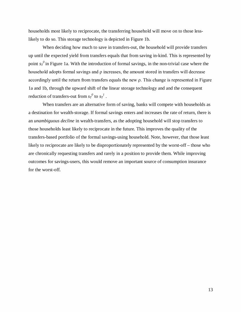
represented in Figure 1a. The introduction of formal savings can be represents a new storage

technology. Let sB represent the amount saved through formal accounts, and assume that the

return from this form of saving is also linear. The introduction of this new savings technology is

represented in Figure 1c.

If formal savings is a superior savings technology, its introduction will cause the overall

return on savings ρ to increase. This may happen, for example, through a reduction in the

transaction-costs of saving and dissaving if formal accounts represent a more liquid technology.

Purchasing and liquidating non-financial assets such as bicycles, radios, or goats may entail

substantial time-costs of searching for a buyer, which may take several hours, days, or even

12

weeks. There may also be explicit travel or transport costs involved in finding a buyer or seller,

or transporting the asset. There will also be search and possibly transport costs for finding a new

(lower-valued) non-financial asset in order to store the remainder of the precautionary savings

the assisting household wants to hold. There may also be losses in asset-value that could come

from having to sell the asset at an inopportune time, or with an urgency that prevents getting the

best price.7

If the rate of return on formal savings is lower than that of saving through durables, the

household will continue to save through durables and not start using formal savings. However, if

the return on formal savings is higher, the household will switch to formal savings, and the return

on its savings will increase. This is the case depicted in Figure 1c.

Storing and accessing wealth through formal accounts has a different set of

transaction costs – e.g. traveling to the bank, any withdrawal fees – yet it is likely these will be

lower. Formal savings may also have positive amounts of interest not available from saving in-

kind, and lower risk of theft, loss, or damage.

Case 1: Transfers as “Saving Through People”

If transfers are best understood as an alternative form of saving to insure against future

shocks, a request by another for help is interpreted as an opportunity to save. In contrast to non-

financial assets and formal accounts, it is reasonable to assume that saving through transfers to

people, sT , yields diminishing marginal returns. At any given time, only a fixed number of

people in one’s network or community are likely to desire a transfer from another household.

These households are likely to vary in their probability of being able to reciprocate the transfer at

a future date. A relatively wealthy household, for example, that had an unusually bad year may

be more likely to reciprocate than a very poor household which requests transfers from others

almost every year. Expected future returns from each unit “saved” through a transfer drop for

households with lower probabilities of reciprocating. After making transfers first to those

7For example, in the presence of segmented markets, selling an asset just before harvest when local incomes are low may result in low demand and low prices obtained for the asset, or selling at a time when others are also trying to sell the same asset in order to liquidate their precautionary savings (e.g. due to a covariate shock) may cause a local supply shock and decrease the price received. The asset may have been purchased at a higher price, and would typically be redeemable at that higher price, if the household could wait until the value rose again, before liquidating it. Thus, even without any other costs, it may require a wealth amount which would otherwise be equal to x+z in order to withdraw and use wealth amount x now.

13

households most likely to reciprocate, the transferring household will move on to those less-

likely to do so. This storage technology is depicted in Figure 1b.

When deciding how much to save in transfers-out, the household will provide transfers

up until the expected yield from transfers equals that from saving in-kind. This is represented by

point sT0 in Figure 1a. With the introduction of formal savings, in the non-trivial case where the

household adopts formal savings and ρ increases, the amount stored in transfers will decrease

accordingly until the return from transfers equals the new ρ. This change is represented in Figure

1a and 1b, through the upward shift of the linear storage technology and and the consequent

reduction of transfers-out from sT0 to sT

1 .

When transfers are an alternative form of saving, banks will compete with households as

a destination for wealth-storage. If formal savings enters and increases the rate of return, there is

an unambiguous decline in wealth-transfers, as the adopting household will stop transfers to

those households least likely to reciprocate in the future. This improves the quality of the

transfers-based portfolio of the formal savings-using household. Note, however, that those least

likely to reciprocate are likely to be disproportionately represented by the worst-off – those who

are chronically requesting transfers and rarely in a position to provide them. While improving

outcomes for savings-users, this would remove an important source of consumption insurance

for the worst-off.

14

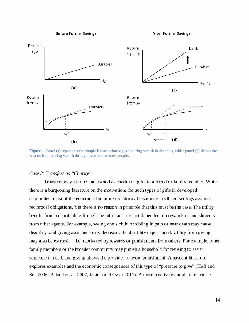
Figure 1. Panel (a) represents the simple linear technology of storing wealth in durables, while panel (b) shows the returns from storing wealth through transfers to other people.

Case 2: Transfers as “Charity”

Transfers may also be understood as charitable gifts to a friend or family member. While

there is a burgeoning literature on the motivations for such types of gifts in developed

economies, most of the economic literature on informal insurance in village-settings assumes

reciprocal obligations. Yet there is no reason in principle that this must be the case. The utility

benefit from a charitable gift might be intrinsic – i.e. not dependent on rewards or punishments

from other agents. For example, seeing one’s child or sibling in pain or near death may cause

disutility, and giving assistance may decreases the disutility experienced. Utility from giving

may also be extrinsic – i.e. motivated by rewards or punishments from others. For example, other

family members or the broader community may punish a household for refusing to assist

someone in need, and giving allows the provider to avoid punishment. A nascent literature

explores examples and the economic consequences of this type of “pressure to give” (Hoff and

Sen 2006, Baland et. al. 2007, Jakiela and Ozier 2011). A more positive example of extrinsic

15

utility would be that being requested for a gift provides the opportunity to earn utility-enhancing

respect and admiration in the community by providing assistance.

In this case, assume that utility includes both consumption c and transfers x as arguments,

so that , and that first derivatives are positive for both arguments and the second

derivatives negative for both arguments. Furthermore, assume they are neither complements nor

substitutes (i.e. the cross-partials are zero). Transfers-out may therefore be understood simply as

a different type of consumption, the marginal value of which is unaffected by own-consumption

levels. Assume that income each period is exogenous to choices over consumption and

charitable transfers, and that utility each period is additively separable. Then the household’s

decision about how to allocate its resources can be explained with the following simple two-

period model:

where ci represents consumption in each period, xi represents a charitable gift in each period, yi is

income received each period, δ is a discount factor, and ρ is the rate of return on savings.

In this setting, an increase in the interest rate will have the standard result that future

consumption will increase, while the effect in present-period consumption is ambiguous. That is,

as the rate of return on savings goes up, there is both a substitution effect and an income effect.

The substitution effect causes the household to substitute away from c1 and x1 towards c2 and

x2, as the relative price of the latter two drop. The real price of future expenditures (whether on c2

or x2), in terms of present expenditures, becomes cheaper – each unit of future c2 (or x2)

requires a smaller sacrifice of current c1 (or x1) as ρ increases. However, the income effect

causes consumption and gifts in both periods to increase. The overall effect for period 2 is

positive, but is ambiguous in period 1. While consuming and giving in the present period is now

more costly in terms of future potential consumption and giving sacrificed, it is also possible to

increase both present consumption and giving and future consumption and giving. The effect of

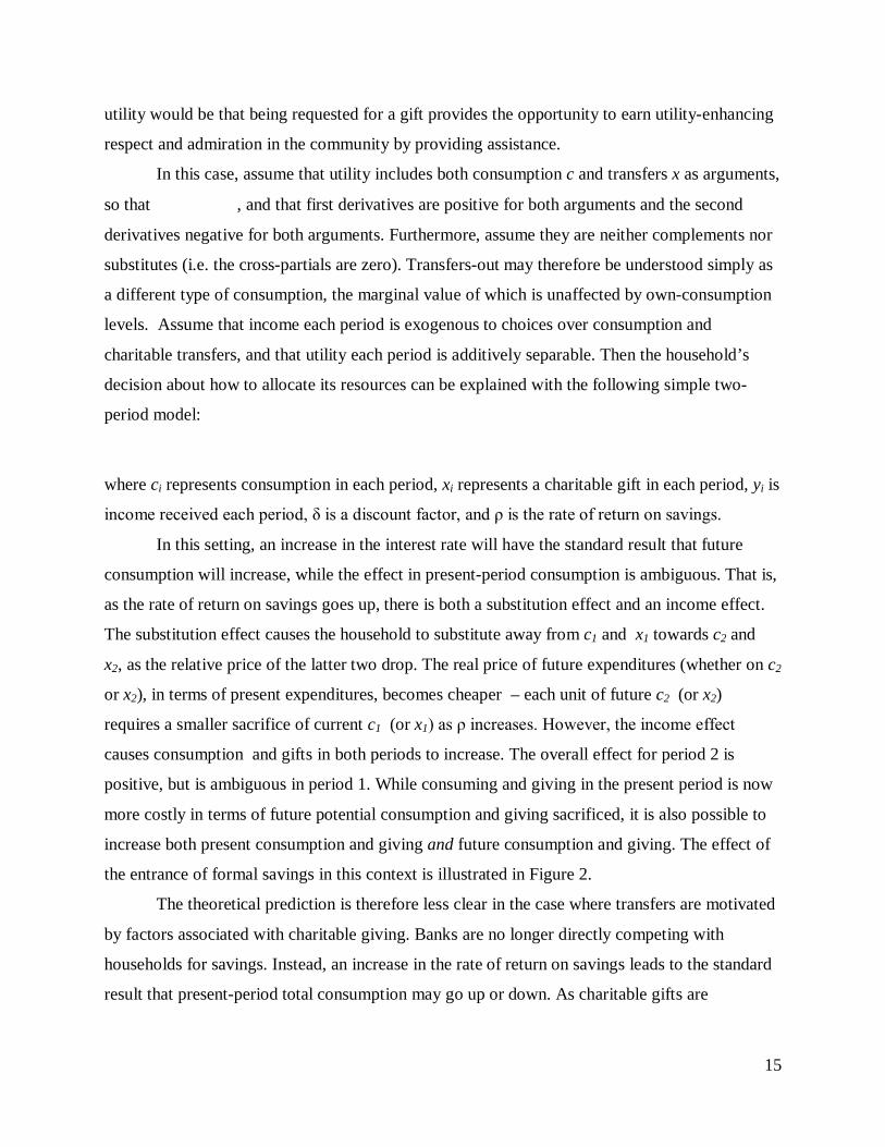
the entrance of formal savings in this context is illustrated in Figure 2.

The theoretical prediction is therefore less clear in the case where transfers are motivated

by factors associated with charitable giving. Banks are no longer directly competing with

households for savings. Instead, an increase in the rate of return on savings leads to the standard

result that present-period total consumption may go up or down. As charitable gifts are

16

essentially another type of consumption, they may also either go up or down as the rate of return

on savings increases.

Figure 2: Panel a shows the simple linear savings technology represented by saving in durables. Panel b shows…

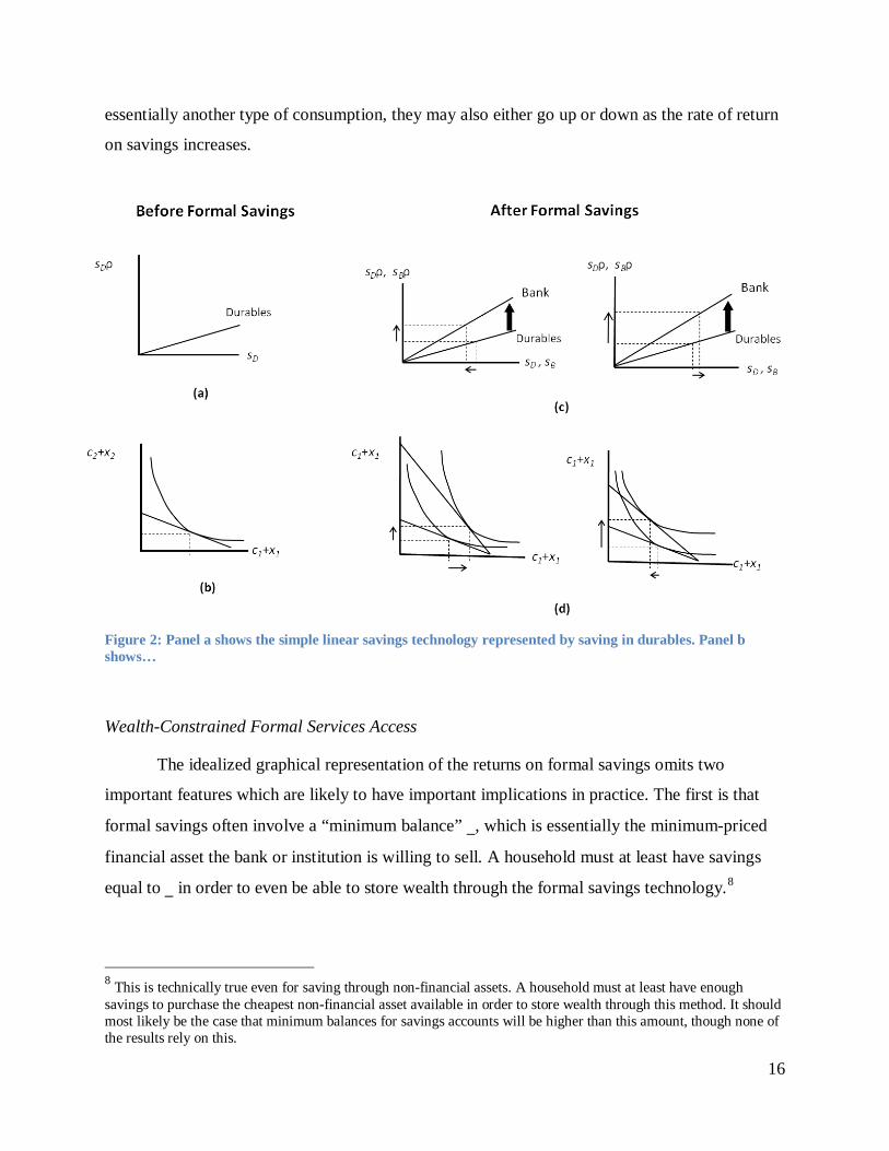
Wealth-Constrained Formal Services Access

The idealized graphical representation of the returns on formal savings omits two

important features which are likely to have important implications in practice. The first is that

formal savings often involve a “minimum balance” , which is essentially the minimum-priced

financial asset the bank or institution is willing to sell. A household must at least have savings

equal to in order to even be able to store wealth through the formal savings technology.8

8 This is technically true even for saving through non-financial assets. A household must at least have enough savings to purchase the cheapest non-financial asset available in order to store wealth through this method. It should most likely be the case that minimum balances for savings accounts will be higher than this amount, though none of the results rely on this.

17

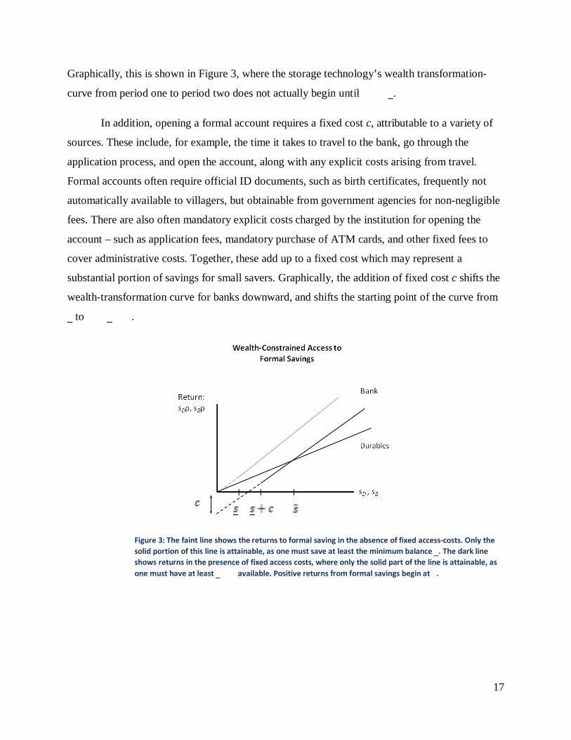
Graphically, this is shown in Figure 3, where the storage technology’s wealth transformation-

curve from period one to period two does not actually begin until .

In addition, opening a formal account requires a fixed cost c, attributable to a variety of

sources. These include, for example, the time it takes to travel to the bank, go through the

application process, and open the account, along with any explicit costs arising from travel.

Formal accounts often require official ID documents, such as birth certificates, frequently not

automatically available to villagers, but obtainable from government agencies for non-negligible

fees. There are also often mandatory explicit costs charged by the institution for opening the

account – such as application fees, mandatory purchase of ATM cards, and other fixed fees to

cover administrative costs. Together, these add up to a fixed cost which may represent a

substantial portion of savings for small savers. Graphically, the addition of fixed cost c shifts the

wealth-transformation curve for banks downward, and shifts the starting point of the curve from

to .

Figure 3: The faint line shows the returns to formal saving in the absence of fixed access-costs. Only the solid portion of this line is attainable, as one must save at least the minimum balance . The dark line shows returns in the presence of fixed access costs, where only the solid part of the line is attainable, as one must have at least available. Positive returns from formal savings begin at .

18

Thus, only those households that are able to save at least even have the ability

to gain access to formal savings.9

The question then becomes whether they experience any indirect effects as a result of the

fact that the comparatively “wealthy” in their community – from whom the poorest might request

transfers in times of need – start using formal savings. The theoretical framework suggests this

depends on three factors: whether the relatively wealthy generally provide assistance to the

worst-off prior to the introduction of formal savings; if so, whether such transfers are assumed to

be based on the promise of reciprocation or instead driven by factors associated with charitable

giving; and if the latter, whether the income effect dominates the substitution effect.

This makes the poorest segments of the population essentially

ineligible to adopt use of formal savings. The poorest in village communities are therefore

unlikely to open savings accounts at banks, and thus unlikely to experience direct benefits from

the expansion of formal savings services.

While the model focuses on giving behavior of account-adopters, the empirical analysis

that follows focuses primarily on the effects of local formal savings adoption on receipts of

assistance. Focusing on assistance receipts (rather than gifts-out) places the analysis squarely on

one of the most sensitive issues for poverty policy: whether and how formal savings expansion

affects non-users, and in particular, the most vulnerable members of the community. This

indirect approach to testing the model is also partly a response to the empirical challenge

presented by the data. Many communities are likely to have comparatively few households

wealthy enough to access and derive positive returns from formal savings, and hence relatively

few initial service-adopters. It is reasonable to suppose that when the relatively wealthy in a

village provide assistance, they give to multiple households. A random sample from this

environment is therefore likely to have more households that are potential recipients from formal

savings adopters than households that are account-adopters. This means that tests on the behavior

of adopting households are likely to lack statistical power. Tests on receipts of wealth flows in

communities with high rates of adoption, however, serve as indirect evidence of the effects on

decisions over transfers out.

9 Also note that, given that the fixed cost causes the total return from savings to drop, it is possible that saving amount no longer provides a higher return than saving through durables. It may be necessary to save at least through formal savings in order for the total return to be higher than the pre-existing alternatives.

19

4. Empirical Setting, The Data, and Identification Strategy

The south-central African nation of Malawi presents an environment well-suited to test

the empirical effects of the introduction of formal savings vehicles to rural areas of the

developing world. It is one of the poorest countries, has low levels of infrastructure, and low

participation in formal financial markets among the rural populace.10 On the other hand, the data

confirm significant incidence of inter-household assistance, gifts, and loans.11

To address the low rates of formal financial service penetration, starting in late 2007, a

local microfinance organization began a project to expand access to formal savings and credit

services to rural areas. The expansion occurred through a mobile van-bank innovation, rolled out

in the three largest districts of central Malawi – Lilongwe, Mchinji, and Dedza districts. The

mobile bank traveled along paved roads, and had six different stops – three stops along the main

highway running 110 km west from the capital city of Lilongwe (located in the center of

Lilongwe district), and three stops along the main highway running 90 km south. The stops were

located in trading centers, and the bank stopped at each one on the same day every week –

usually a market day, in order to take advantage of the fact that many villagers from surrounding

areas are already in the trading center for other reasons. This not only reduces the transportation

component of transaction costs, but also catches people after making sales, when they are more

likely to have cash on hand to deposit into savings accounts.

This expansion of formal services into the relatively thin financial environment of rural

Malawi provides an ideal opportunity to better understand the interaction between formal savings

markets and local indigenous safety-net systems. The data, a two-year panel that spans the initial

phases of the expansion of access, come from a household survey forming part of an independent

impact assessment of the microfinance organization’s services on client-household welfares.12

10 In 2008, 6.0% of the sampled households had at least one current formal loan, while 11.6% of the households had one or more formal savings accounts. Only 2.8% of the sampled households reported both formal savings and formal credit, so about 14.7% of the sample reported using formal savings accounts, formal credit, or both.

The impact assessment’s intent was to determine whether, and by how much, the average user of

11 For example, in 2008, 23.6% of the sampled households reported having at least one current informal loan from a friend or relative. 12 The IRIS Center of the University of Maryland was hired by the Bill and Melinda Gates Foundation to perform an impact assessment evaluating the effect of the bank’s services on client-household vulnerability, food security, and other welfare outcomes.

20

financial services benefited by becoming a client of the microfinance institution. However, this

paper uses the data to examine how the expansion of financial services, and formal savings in

particular, impacts non-service users, with specific emphasis on the highly vulnerable.

Focusing on the poorest households ensures effects detected are through an indirect

channel (since they do not adopt formal services, as their extreme poverty makes them

essentially ineligible), and also places the analysis squarely on a population of crucial importance

for poverty policy – the poorest of the poor. The microfinance organization follows a protocol

that constrains its expansion of access to loans in a manner uncorrelated with the instrument I use

for formal savings-adoption. Thus, expansion of credit access in the area follows a path

orthogonal to the exogenously boosted uptake of formal savings services.13

The baseline data was collected over February-April of 2008, during the pre-harvest

“hungry” season when food-stocks tend to be low for the most vulnerable households. This was

before any significant take-up of the microfinance organization’s services. While the mobile van-

bank first began operations in August of 2007, there was little to no marketing, awareness of the

existence of the mobile bank was low, and it was already well after the high-income harvest

period when people are comparatively flush with cash.

14 15

Community sampling was performed following a matched-pair design. Each pair

consisted of two village-clusters, a cluster being defined by enumeration areas (EAs) – sampling

units defined by Malawi’s National Statistics Office that typically include 2-4 villages

The second round of data was

collected during the same period of 2010, following two years of intensive marketing of the

bank’s services.

16

13 Access to loans is expanded village-by-village, as the microfinance organization develops relationships with local leaders. Credit access therefore follows a path that is independent from the uptake of savings services. The intensive marketing is therefore likely to have an effect purely on savings uptake, and not on loans. This is in fact confirmed in the endline data, which shows differences in savings-account openings, but not in formal credit.

. Clusters

of villages were first categorized based on distance from the mobile van-bank stop: (i) within

5km; (ii) 5-10 km; (iii) more than 10 km. They were then further split into two population

categories: high versus low. Two clusters (EAs) were then randomly sampled from each

14 Malawi has a single growing season. Most farming households receive the majority of their annual income during one single period of the year – the harvest period, which in Central Malawi usually lasts from late April into June. 15 The low awareness about the existence of the microfinance organization’s mobile van-bank is supported by information collected in focus-group discussions in 2008, and is also confirmed by the very low incidence in the baseline data of households using the organization’s financial services. 16 For very large villages, the EA may consist of only one village; in a few cases, the EA might include as many as 5 villages. Both of these cases are rare in the data.

21

population-distance group to form a pair. A total of 60 pairs were sampled (120 clusters total).

Finally, within each pair, one of the clusters (EAs) was randomly selected to receive the

information treatment to encourage adoption of the bank’s financial services.

Within each cluster (EA), typically 2 to 4 villages were randomly selected for sampling.

Within each village, 6-10 households were randomly selected to be surveyed. Each sampled

cluster contains 20-23 sampled households. Due to unforeseen sampling issues, some data loss,

and complications with the marketing campaign in one location, four pairs had to be dropped.

The final remaining panel contains 112 clusters (about 325 villages), with a total of 2,006

households. Villages are located at radial distances from the mobile bank call-point ranging

between 0 and 14 kilometers.

The Instrument for Formal Savings Adoption: Information Intervention

Since it was not feasible to directly randomize access to the bank’s services, we designed

an encouragement in the form of an intensive information campaign to serve as an instrument for

service take-up. Using information collected during focus group discussions in villages on how

people usually obtain trustworthy information from sources outside the village, we worked with

the microfinance organization to design a marketing campaign that would mirror these methods

of information dissemination. The backbone of the campaign consisted of periodic visits (via

foot and bicycle) to each marketing-village from a paid Field-Based Promotional Assistant

(FBPA) who brought informational materials, talked with members of the community, and left

posters and other promotional materials in each village assigned to the marketing treatment. The

goal was to induce higher take-up rates in the marketing village clusters than in non- marketing

clusters. A restriction that marketing clusters be located at least a few kilometers from non-

marketing clusters helped minimize the possibility that information spillovers from the campaign

into the non-marketing areas might also induce households in the non-marketing areas to adopt

the bank’s services.

The exclusion restriction required for the encouragement to be able to function as a valid

instrument for the effects of financial services use relies on the assumption that the only way

periodic informational visits by bank representatives changed villagers’ behavior, such that it

differed from the non-encouraged clusters, was in their decision about whether to adopt formal

22

services. That is, the validity of the instrument requires that these visits by themselves did not

directly influence the outcomes of interest (e.g. inter-household transfers) through a channel

other than the local uptake of financial services. This would be violated, for example, if the

information intervention directly affected other behaviors in the community besides service-

adoption, or directly altered other community-level variables, in ways that affected the outcomes

of interest. The assumption that the exclusion restriction holds is valid if the only change that the

marketing campaign introduced to marketing areas was to expand individuals’ information sets

and that the only effect of more information was to induce more households to adopt.17

The exclusive goal of the campaign was to provide information on the institution’s

products, with the hope that this would cause households to realize that it was to their benefit to

open up savings accounts. As the bank is a savings-driven institution, its goal was to expand its

client base, and the sole responsibility of FBPAs was to bring in more clients to the bank – i.e.

recruit more formal savers. Their job consisted entirely of teaching locals about financial

products and why they might find those offered by the bank useful.

For the exclusion restriction to be violated, either (i) the information-content itself would

have had to affect choices besides the financial services adoption decision; or (ii) the form the

intervention took – periodic visits by the FBPAs – would have had to introduce elements to the

marketing clusters not also present in the non-marketing clusters. With regard to the second

possibility, it is not clear what visits by the FBPAs would introduce to communities other than

information. Their sole job was to provide information on the bank’s services and recruit new

clients, and they were incentivized to do so as broadly and rapidly as possible. They were also

present in each village only once every few weeks, sometimes only for a few hours,18

It is possible that tangential elements are somehow incidentally introduced by these types

of visits to villages by outsiders from urban areas. Nevertheless, it is unlikely this would have

caused any systematic differences between the encouraged and non-encouraged clusters. Most

of the village clusters (marketing and non-marketing) are all located within 10 km of a major

preoccupied with the goal of teaching, convincing, and recruiting new clients.

17 As discussed elsewhere, one explanation for why more information should lead to adoption of services is that the information intervention can be seen as a random reduction of information-acquisition costs for those in the marketing clusters. 18 The FBPAs typically walked or bicycled to the communities where they worked. Travel times could be as long as a few hours in many cases, which often left only a few hours during the day to interact with community members.

23

highway. The periodic presence of non-locals whose job it is to bring outside information to the

communities is not unusual.19 It is quite common, for example, for agricultural extension

officers and nutrition and health extension officers, to make informational visits to these villages

in order to educate people about new techniques, practices, and available services20. This is just

as true in the non-encouraged clusters as in the encouraged clusters. Insofar as the form it took,

the marketing campaign therefore does not introduce anything new or unusual.21

The second way that the encouragement could have had a direct effect is that the

information-content itself could have somehow affected behaviors other than the financial

services adoption decision. There is no clear reason to expect that more information about formal

financial products would, by itself, lead to changes in inter-household assistance behavior. While

detailed knowledge among those who actually use the services may be relevant to choices about

assisting others (e.g. individuals realize they have higher rates of return by using formal savings),

in most cases knowledge about services should be irrelevant to non-users. In particular, there is

no reason to expect that simply knowing the details about formal savings and credit products

should cause someone who does not use such products to start giving more assistance to others.

Each FBPA

was responsible for as many as 20-30 villages, and as much as a month might pass between

visits. It is therefore unlikely that they could have introduced anything to marketing areas not

also already present in the non-marketing areas – besides the provision of information on

financial services.

To the extent that marketing might contain non-informational components intended to

persuade (framing, etc.), any effects from such components are still likely to only affect the

adoption decision and not have lasting impacts on other behaviors. This is especially true given

the short-term and infrequent nature of the visits by FBPAs. While any aspects of the marketing

19 This is actually a nice virtue of fashioning the encouragement in the way that we did – it fits right in with other commonly experienced “interventions” in these communities, which minimizes the risk that it did anything new to the marketing-areas (not also being experienced in the non-marketing areas), besides the provision of information on formal financial services. 20 This was, in fact, the primary inspiration for how we designed the encouragement. After learning that this is the standard way that villages commonly receive information from outside, we intentionally fashioned the information intervention to mimic these pre-existing methods. 21 While it might be argued that the campaign does add another set of visits, and this might matter if such visits do indeed have tangential effects, any marginal impact the mere periodic presence of FBPAs might have on local outcomes is minimal compared to decades of visits by government extension workers, aid organizations, and others. In addition, for this to have any bearing on the exclusion restriction’s validity, it would have to be the case that these visits not only have some effect, but have an effect on the outcomes of interest.

24

that might have been more subjective or emotive could conceivably influence a decision of

whether to adopt, they are unlikely to have lasting influences on long-standing personal habits or

responses to the pressure of engrained social norms.

Even if non-informational components of the marketing did somehow have lasting direct

effects on behavior, they would likely be in the opposite direction of the effects I find. It is

perhaps possible, for example, that the bank’s implicit – and often explicit – emphasis on the

importance of building one’s own personal wealth as an avenue to financial independence and

future personal prosperity might be passed on by the FBPAs and operate as an ideological

influence on behavior.22

This could potentially influence the behavior of all households in the

community – regardless of whether they start using formal services – encouraging them to share

less and focus more on the accumulation of personal or household cash resources and other

assets. Again, however, it is unlikely that a handful of visits to the community over several

months would be enough for ideology to have a large or immediate impact on long-standing

social practices and individual habits. Nevertheless, to the extent that this is a possibility, such an

effect would bias estimated impacts of formal savings uptake towards less assistance to other

households. This would make it even harder to detect the patterns I find in the data, and would

therefore suggest my findings are a lower bound of the true effects.

Baseline Descriptive Statistics, Overall & by Marketing/Non-Marketing Areas

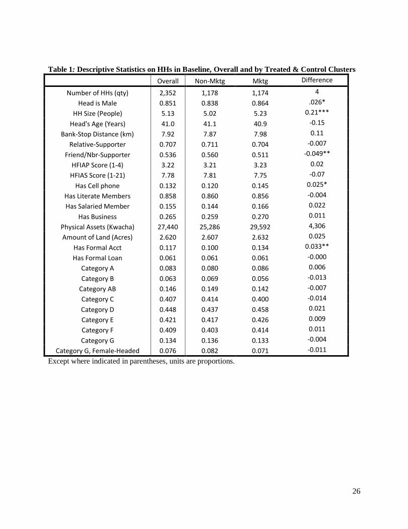
Table 1 reports descriptive statistics on several important household dimensions of the

baseline sample, restricted to the 56 treatment-control pairs in the final sample. As the statistics

are from the baseline sample, it includes the 341 households that attrited and which are not part

of the final full panel. The table presents overall figures, then split by marketing and non-

marketing. The variable “Relative Supporter” is a dummy for whether the household reported in

the baseline that they can rely on a relative for support in times of need, and the variable

“Friend/Nbr Supporter” is a dummy for whether they reported in the baseline being able to rely

22 Such an affect would be at the level of altering preferences themselves. While not entirely outside the realm of possibility, this type of effect would most likely require much more frequent and extended exposure in order for new ways of thinking to counter long-standing social practices and individual habits.

25

on a friend or neighbor. The HFIAP-Score is a 4-point food-security indicator that forms the

basis for vulnerability-categories. The HFIAS-score is a 21-point food-security indicator. (For

both indicators, higher values imply less security.) Category A through Category G are

household vulnerability indicators, defined in the next section, such that these take a value of 1

if the household belongs to the category. Unless otherwise indicated, the reported values are

percentages of households in the sample for which the indicator variable is true. The column of

differences indicates statistically significant differences based on two-sided t-tests, with standard

levels of significance indicated.

26

Table 1: Descriptive Statistics on HHs in Baseline, Overall and by Treated & Control Clusters

Overall Non-Mktg Mktg Difference

Number of HHs (qty) 2,352 1,178 1,174 4

Head is Male 0.851 0.838 0.864 .026*

HH Size (People) 5.13 5.02 5.23 0.21***

Head's Age (Years) 41.0 41.1 40.9 -0.15

Bank-Stop Distance (km) 7.92 7.87 7.98 0.11

Relative-Supporter 0.707 0.711 0.704 -0.007

Friend/Nbr-Supporter 0.536 0.560 0.511 -0.049**

HFIAP Score (1-4) 3.22 3.21 3.23 0.02

HFIAS Score (1-21) 7.78 7.81 7.75 -0.07

Has Cell phone 0.132 0.120 0.145 0.025*

Has Literate Members 0.858 0.860 0.856 -0.004

Has Salaried Member 0.155 0.144 0.166 0.022

Has Business 0.265 0.259 0.270 0.011

Physical Assets (Kwacha) 27,440 25,286 29,592 4,306

Amount of Land (Acres) 2.620 2.607 2.632 0.025

Has Formal Acct 0.117 0.100 0.134 0.033**

Has Formal Loan 0.061 0.061 0.061 -0.000

Category A 0.083 0.080 0.086 0.006

Category B 0.063 0.069 0.056 -0.013

Category AB 0.146 0.149 0.142 -0.007

Category C 0.407 0.414 0.400 -0.014

Category D 0.448 0.437 0.458 0.021

Category E 0.421 0.417 0.426 0.009

Category F 0.409 0.403 0.414 0.011

Category G 0.134 0.136 0.133 -0.004

Category G, Female-Headed 0.076 0.082 0.071 -0.011

Except where indicated in parentheses, units are proportions.

27

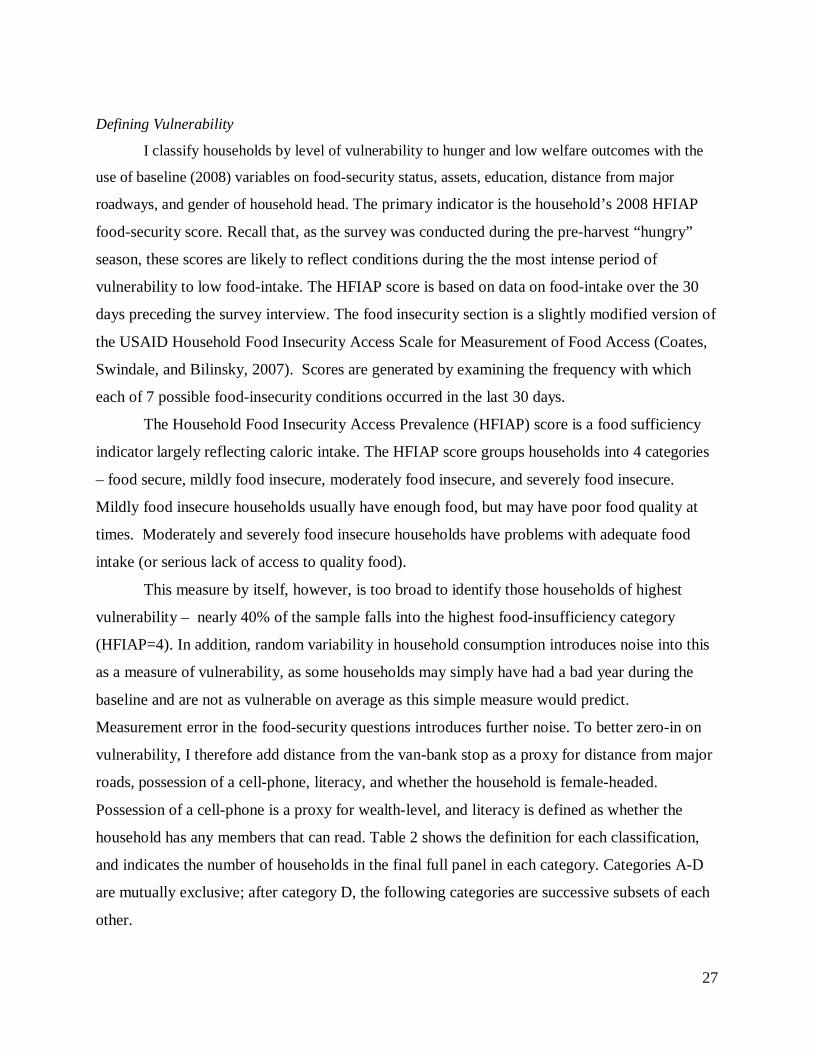
Defining Vulnerability

I classify households by level of vulnerability to hunger and low welfare outcomes with the

use of baseline (2008) variables on food-security status, assets, education, distance from major

roadways, and gender of household head. The primary indicator is the household’s 2008 HFIAP

food-security score. Recall that, as the survey was conducted during the pre-harvest “hungry”

season, these scores are likely to reflect conditions during the the most intense period of

vulnerability to low food-intake. The HFIAP score is based on data on food-intake over the 30

days preceding the survey interview. The food insecurity section is a slightly modified version of

the USAID Household Food Insecurity Access Scale for Measurement of Food Access (Coates,

Swindale, and Bilinsky, 2007). Scores are generated by examining the frequency with which

each of 7 possible food-insecurity conditions occurred in the last 30 days.

The Household Food Insecurity Access Prevalence (HFIAP) score is a food sufficiency

indicator largely reflecting caloric intake. The HFIAP score groups households into 4 categories

– food secure, mildly food insecure, moderately food insecure, and severely food insecure.

Mildly food insecure households usually have enough food, but may have poor food quality at

times. Moderately and severely food insecure households have problems with adequate food

intake (or serious lack of access to quality food).

This measure by itself, however, is too broad to identify those households of highest

vulnerability – nearly 40% of the sample falls into the highest food-insufficiency category

(HFIAP=4). In addition, random variability in household consumption introduces noise into this

as a measure of vulnerability, as some households may simply have had a bad year during the

baseline and are not as vulnerable on average as this simple measure would predict.

Measurement error in the food-security questions introduces further noise. To better zero-in on

vulnerability, I therefore add distance from the van-bank stop as a proxy for distance from major

roads, possession of a cell-phone, literacy, and whether the household is female-headed.

Possession of a cell-phone is a proxy for wealth-level, and literacy is defined as whether the

household has any members that can read. Table 2 shows the definition for each classification,

and indicates the number of households in the final full panel in each category. Categories A-D

are mutually exclusive; after category D, the following categories are successive subsets of each

other.

28

Table 2: Definition of Vulnerability Categories

Vulnerability Category

Definition No. of C-HHs

No. of T-HHs

Category A 2008 HFIAP = 1 Household classified as “food-secure” in 2008.

77 80

Category B 2008 HFIAP = 2 Classified as “mildly food-insecure” in 2008.

61 55

Category AB Category A & B Combined 138 135 Category C 2008 HFIAP = 3

Classified as “moderately food-insecure” in 2008. 417 413

Category D 2008 HFIAP = 4 Classified as “severely food-insecure” in 2008.

443 463

Category E 2008 HFIAP = 4, 3+km Classified as “severely food-insecure” in 2008, located 3 or more kilometers from the bus-bank stop.

429 434

Category F 2008 HFIAP = 4, 3+km, no cell phone Classified as “severely food-insecure” in 2008, located 3 or more kilometers from the bus-bank stop, does not have cell-phone

415 427

Category G 2008 HFIAP = 4, 3+km, no cell phone, illiterate Classified as “severely food-insecure” in 2008, located 3 or more kilometers from the bus-bank stop, does not have cell-phone, and either: (i) no HH member is literate in Chichewa; or (ii) household head is female.

141 131

Note that A,B,C, and D are are mutually exclusive. But E is a subset of D, F is a subset of E, and G is a subset of F.

29

5. Assessing the Instrument: Effects on Local Formal Financial Services Use

I now move on to analysis of the instrument’s effects on financial services use. The

information intervention’s anticipated effect was to increase use of a particular organization’s

financial services among households in the community. However, since the information

provided might also induce individuals to start using services of other financial organizations

near the area, and my goal is to investigate the impact of formal services in general (rather than

those of a specific organization), I look at changes in savings and credit use at any financial

organization.

I first examine the instrument’s effect on adoption and disadoption separately, under

the hypothesis that increased local financial services usage due to new-adopters has different

effects than (prevented) decreased usage among the already-users. This would be the case,

for example, if formal services use affects the behavior of households that had already (pre-

marketing) self-selected into service-use differently than it affects households exogenously

encouraged into its use (e.g. they are systematically different types of households, and

formal services use affects their behavior differently). In the second set of analyses,

however, I ignore this possibility, and look only at the effects of the instrument on the local

prevalence of formal services use (ignoring whether it is from prevented disadoption among

already-users or adoption among previous non-users). The latter may be a simpler approach,

though as will be seen, it raises some complications.

Table 4 below reports results from a simple OLS regression of the adoption (or quitting)

of formal savings services on a dummy indicating assignment to intensive marketing, with fixed

effects at the cluster-pair level, and standard errors clustered at the village-cluster level.23

23Pairs were sampled on the basis of common characteristics, and it is plausible that the different pairs experience the expansion of formal services access via the van-bank differently. For example, those located closer to major highways may be more responsive to the expanded access than those pairs that are further away, regardless of whether they encouraged or non-encouraged.

The

left-hand side variable is a simple 0-1 indicator for whether the household has at least one

formal savings account in 2010. This is equivalent to regressing the mean of the response

variable for each cluster (i.e. the percentage of households in the cluster with formal savings) on

30

the dummy for information intervention, accounting for pair-level fixed effects, and explicitly

correcting for heteroskedasticity across clusters due to the variation in number of households

(FGLS).

Columns 1 and 2 show results when the sample is restricted to those households which

did not have formal savings accounts in 2008. The estimated coefficient for the marketing

dummy therefore represents the increase in the proportion of previous non-savings users that

adopt savings, due to the marketing campaign. The first specification (column 1) includes all

village-clusters, regardless of distance from the van-bank’s stop (including being located right at

the stop). The second (column 2) restricts the sample to those clusters for which both members

of the cluster-pair are located three or more kilometers from the closest van-bank’s stop. The

rationale for splitting the sample in this manner is that the intensive marketing campaign

may have smaller effects in areas close to the bank’s stop, since such households are likely

to already have a high degree of information about the bank and its services, due to living in

close proximity to its regular weekly location.

For the other two specifications, the sample is restricted to those households which did

have at least one formal savings account in 2008. Here, if the dependent variable takes a value of

zero, it means the previously formal-saving household stopped use of formal savings sometime

over the two-year period. Here, the coefficient on the dummy represents any effect the

marketing instrument had on the proportion of previously using households that stopped formal

savings use.

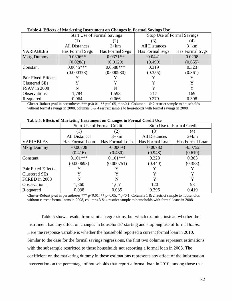
The results in columns 1 and 2 indicate the marketing instrument had a significant effect

on the proportion of previous non-saving households that adopted formal savings, significant at

the .05-level. . Note that both the magnitude and significance of the instrument’s estimated

effect on adoption increases with distance from the bank-stop, which is consistent with the

expectation that information on services is increasingly effective in more remote locations.

Among all clusters, the marketing increased the percentage of previous non-saving

households that adopted by about 3.1% (p=.03), while among clusters three or more

kilometers away, the effect is an increase of 3.7% (p=.01). To put these figures in context, the

overall proportion of previously non-saving households that adopted formal savings in the non-

encouraged clusters is 9.4%. So these changes represent a 33% increase and 40% increase

respectively. The results shown in columns 3 and 4 reveal that marketing encouragement had

31

no significant effect on the proportion of previously saving households that ceased use of

formal savings accounts over the two-year period.

32

Table 4. Effects of Marketing Instrument on Changes in Formal Savings Use Start Use of Formal Savings Stop Use of Formal Savings (1)

All Distances (2)

3+km (3)

All Distances (4)

3+km VARIABLES Has Formal Svgs Has Formal Svgs Has Formal Svgs Has Formal Svgs Mktg Dummy 0.0306** 0.0371** 0.0441 0.0298 (0.0288) (0.0129) (0.490) (0.655) Constant 0.0645*** 0.0588*** 0.319 0.323 (0.000373) (0.000980) (0.355) (0.361) Pair Fixed Effects Y Y Y Y Clustered SEs Y Y Y Y FSAV in 2008 N N Y Y Observations 1,784 1,593 217 169 R-squared 0.064 0.066 0.270 0.308

Cluster-Robust pval in parentheses *** p<0.01, ** p<0.05, * p<0.1. Columns 1 & 2 restrict sample to households without formal savings in 2008, columns 3 & 4 restrict sample to households with formal savings in 2008.

Table 5. Effects of Marketing Instrument on Changes in Formal Credit Use Start Use of Formal Credit Stop Use of Formal Credit (1)

All Distances (2)

3+km (3)

All Distances (4)

3+km VARIABLES Has Formal Loan Has Formal Loan Has Formal Loan Has Formal Loan Mktg Dummy -0.00708 -0.00693 0.00782 -0.0752 (0.416) (0.430) (0.948) (0.619) Constant 0.101*** 0.101*** 0.328 0.383 (0.000693) (0.000751) (0.440) (0.353) Pair Fixed Effects Y Y Y Y Clustered SEs Y Y Y Y FCRED in 2008 N N Y Y Observations 1,860 1,651 120 93 R-squared 0.038 0.035 0.396 0.419

Cluster-Robust pval in parentheses *** p<0.01, ** p<0.05, * p<0.1. Columns 1 & 2 restrict sample to households without current formal loans in 2008, columns 3 & 4 restrict sample to households with formal loans in 2008.

Table 5 shows results from similar regressions, but which examine instead whether the

instrument had any effect on changes in households’ starting and stopping use of formal loans.

Here the response variable is whether the household reported a current formal loan in 2010.

Similar to the case for the formal savings regressions, the first two columns represent estimations

with the subsample restricted to those households not reporting a formal loan in 2008. The

coefficient on the marketing dummy in these estimations represents any effect of the information

intervention on the percentage of households that report a formal loan in 2010, among those that

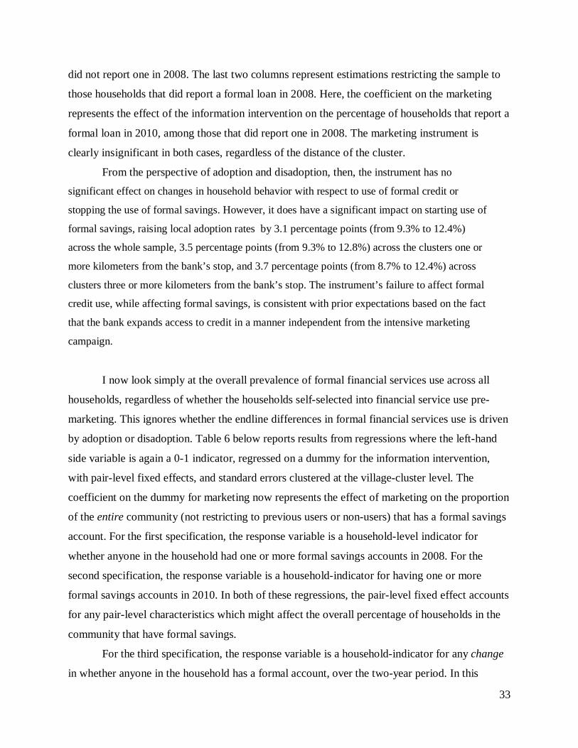
33

did not report one in 2008. The last two columns represent estimations restricting the sample to

those households that did report a formal loan in 2008. Here, the coefficient on the marketing

represents the effect of the information intervention on the percentage of households that report a

formal loan in 2010, among those that did report one in 2008. The marketing instrument is

clearly insignificant in both cases, regardless of the distance of the cluster.

From the perspective of adoption and disadoption, then, the instrument has no

significant effect on changes in household behavior with respect to use of formal credit or

stopping the use of formal savings. However, it does have a significant impact on starting use of

formal savings, raising local adoption rates by 3.1 percentage points (from 9.3% to 12.4%)

across the whole sample, 3.5 percentage points (from 9.3% to 12.8%) across the clusters one or

more kilometers from the bank’s stop, and 3.7 percentage points (from 8.7% to 12.4%) across

clusters three or more kilometers from the bank’s stop. The instrument’s failure to affect formal

credit use, while affecting formal savings, is consistent with prior expectations based on the fact

that the bank expands access to credit in a manner independent from the intensive marketing

campaign.

I now look simply at the overall prevalence of formal financial services use across all

households, regardless of whether the households self-selected into financial service use pre-

marketing. This ignores whether the endline differences in formal financial services use is driven

by adoption or disadoption. Table 6 below reports results from regressions where the left-hand

side variable is again a 0-1 indicator, regressed on a dummy for the information intervention,

with pair-level fixed effects, and standard errors clustered at the village-cluster level. The

coefficient on the dummy for marketing now represents the effect of marketing on the proportion

of the entire community (not restricting to previous users or non-users) that has a formal savings

account. For the first specification, the response variable is a household-level indicator for

whether anyone in the household had one or more formal savings accounts in 2008. For the

second specification, the response variable is a household-indicator for having one or more

formal savings accounts in 2010. In both of these regressions, the pair-level fixed effect accounts

for any pair-level characteristics which might affect the overall percentage of households in the

community that have formal savings.

For the third specification, the response variable is a household-indicator for any change

in whether anyone in the household has a formal account, over the two-year period. In this

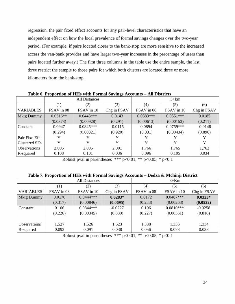
34

regression, the pair fixed effect accounts for any pair-level characteristics that have an

independent effect on how the local prevalence of formal savings changes over the two-year

period. (For example, if pairs located closer to the bank-stop are more sensitive to the increased

access the van-bank provides and have larger two-year increases in the percentage of users than

pairs located further away.) The first three columns in the table use the entire sample, the last

three restrict the sample to those pairs for which both clusters are located three or more

kilometers from the bank-stop.

Table 6. Proportion of HHs with Formal Savings Accounts – All Districts All Distances 3+km (1) (2) (3) (4) (5) (6) VARIABLES FSAV in 08 FSAV in 10 Chg in FSAV FSAV in 08 FSAV in 10 Chg in FSAV Mktg Dummy 0.0316** 0.0443*** 0.0143 0.0383*** 0.0551*** 0.0185 (0.0373) (0.00928) (0.291) (0.00613) (0.00153) (0.211) Constant 0.0947 0.0845*** -0.0115 0.0894 0.0759*** -0.0148 (0.294) (0.00321) (0.920) (0.331) (0.00434) (0.896) Pair Fixd Eff Y Y Y Y Y Y Clustered SEs Y Y Y Y Y Y Observations 2,005 2,005 2,001 1,766 1,765 1,762 R-squared 0.108 0.101 0.036 0.096 0.105 0.034

Robust pval in parentheses *** p<0.01, ** p<0.05, * p<0.1 Table 7. Proportion of HHs with Formal Savings Accounts – Dedza & Mchinji District

All Distances 3+Km (1) (2) (3) (4) (5) (6) VARIABLES FSAV in 08 FSAV in 10 Chg in FSAV FSAV in 08 FSAV in 10 Chg in FSAV Mktg Dummy 0.0170 0.0444*** 0.0283* 0.0172 0.0487*** 0.0323* (0.317) (0.00846) (0.0695) (0.233) (0.00268) (0.0522) Constant 0.106 0.0844*** -0.0227 0.106 0.0810*** -0.0258 (0.226) (0.00345) (0.839) (0.227) (0.00361) (0.816) Observations 1,527 1,526 1,523 1,338 1,336 1,334 R-squared 0.093 0.091 0.038 0.056 0.078 0.038

Robust pval in parentheses *** p<0.01, ** p<0.05, * p<0.1

35

The first thing to note in Table 6 is that the marketing instrument appears to have no

significant effect on the change in the overall percentage of households in the community with

formal savings, even when restricting to the more remote distance threshold where the

instrument is more effective. This is initially worrying. Just as worrying is the fact that it appears

that formal savings was already more prevalent in the marketing clusters than the non-marketing

clusters prior to the marketing campaign. It would seem that, while the randomization was

successful at achieving a balance between encouraged and non-encouraged clusters along most

household dimensions, it failed to achieve a balance in prevalence of formal savings use.

However, upon closer examination of the data, the higher pre-intervention incidence of

formal savings in the encouraged areas does not appear to be systematic. It is driven by

differences in Lilongwe district – particularly from the upper tail of the distribution. For almost

all (90%) of the 27 village clusters in Lilongwe district, the reported baseline percentage of

households with formal savings accounts was 25% or lower (the mean was 12.7%). However,

three clusters had levels of incidence reported at 43% or higher (43%, 50%, and 55%). All three

of these outliers happened to be assigned to receive the information intervention. The matched

village cluster which happened to be assigned to control for each had proportions of 0%, 14%

and 25%, respectively. Assuming the randomly assigned status was independent across each

matched pair, the probability that this would occur is .125, low but clearly plausible. Given the

skewed distribution of formal savings prevalence in Lilongwe, it would appear we were unlucky

with the randomization.24

It also turns out that the effect of marketing on the change in prevalence of formal

savings over the 2-year period is not significant in Lilongwe, and is in fact mildly negative. This

might be due to the fact that households in Lilongwe district are closer to the capital city (and the

bank’s headquarters), and may have better access to information and higher frequency of visits to

the capital.

Another possibility is that I have not specified the model for the change in percentage

appropriately. There is good reason to believe the initial level of financial services prevalence 24 Had the randomization resulted in opposite assignment within just the first pair alone (the one for which the difference is 43% vs. 0%), the baseline difference in formal savings rates across treated and non-treated communities would disappear entirely. The coefficient on the marketing dummy for proportion of the cluster with formal savings would have a t-statistic of 0.93 (p=.354).

36

also affects the rate of expansion. Just as can be the case in other types of technology adoption,

use of technology by relatives and neighbors may spur the use of adoption by new users, such

that the rate of expansion will be higher among those communities that already have

comparatively higher rates of penetration, and lower among those communities with very low

penetration (or communities with none at all). For example, in villages where no one has ever

had a formal savings account, people may be much more suspicious of its utility – and even the

security of their savings – whereas in villages where a quarter of the population has already

recently started using formal savings, non-users may be less reluctant to start.

It is plausible that the initial-period level of formal savings prevalence (the percentage of

households in the community with formal savings accounts) should affect the rate of change, via

two possible opposite effects. First, if adoption exhibits any “learning by observing” or

“copying” patterns, or if community members have increasing trust as they see more neighbors

using formal financial services, one would expect higher period-one prevalence rates to lead to

higher two-year changes in the prevalence in that area. For example, a community with only 1%

of the population using formal services may take many years to reach a penetration rate of 5%

without any outside intervention, simply due to very low local levels of awareness and/or trust

with regard to the services. On the other hand, a community that starts out with penetration rates

of 15% might reach a prevalence rate of 20% or 25% within just one or two years, as more and

more people notice, trust, learn about the services and the benefits they would provide.

Secondly, however, it may also be that there is a latent “capacity” within a community

for the penetration rate of formal services, determined by the wealth levels of its inhabitants. If a

substantial portion of the population (say X) is below the wealth threshold at which use of formal

services provides net benefits, then one would expect the maximum penetration rate to be 100-X.

It may also be the case that the closer the penetration rate gets to the maximum capacity, the

slower usage spreads, since those (among the population that would actually benefit) who are

last to adopt are likely to be the most resistant and slowest to be convinced. Regardless, the

existence of a latent capacity would cause one to expect that higher period-one prevalence rates

would lead to lower absolute values for the 2-year change in prevalence rate.

37

If either of the above is the case, I should be including in the regressions for change in

percentage of financial service users the initial local level of financial services use.25

Table 7 shows the results when I restrict to these two districts. There is no difference

between marketing and non-marketing clusters in local prevalence of formal savings in the

baseline, but there is a highly significant difference in the endline. The regression on the change

in local prevalence of formal savings shows that the marketing resulted in a 2.8 percentage-point

increase overall (p=.07), and a 3.2 percentage-point increase when restricting to the more remote

village clusters (p=.05). As the average prevalence among non-marketing clusters in the endline

was 12.2% overall and 10.4% in the more remote clusters, this represents a boost in the increase

of local formal saving use by 23% and 31%, respectively.

For the time

being, however, since it may be the case that communities in Lilongwe district are simply less

responsive to the marketing because they are closer to the capital, I restrict the sample to Mchinji

and Dedza districts (76% of the sample) and proceed with the analysis. Appendix _X__ does in

fact show that, when controlling for baseline penetration rates, initial usage levels do have a

significant effect on the change, and the impact of marketing on savings penetration increases

and is significant even in Lilongwe.

I repeat the same estimation exercise for use of formal credit. The response variables in

this case are based on a 0-1 variable for whether a household has a current formal loan. The

results are reported in Tables 8 and 9 below.26

25 It is worth mentioning that a linear regression is not entirely appropriate for a response variable that is a percentage, as it allows for predicted values outside the range of (0,1). I also tried running a Logit on the prevalence of formal savings in the baseline, and found almost identical results on the differences (though a few pairs had to be dropped from the regression). 26 It could be that a more accurate assessment of changes in access to formal credit would involve looking at current and past loans over the intervening two-year period. Appendix X ?? considers the question of changes in formal credit access from this perspective, and yields similar conclusions: the information intervention does not increase usage of formal credit, whether conditioning on baseline formal credit penetration or not.

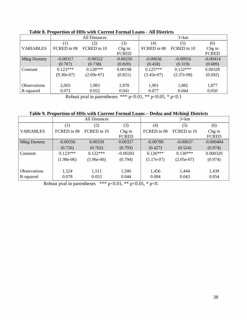
38

Table 8. Proportion of HHs with Current Formal Loans - All Districts All Distances 3+km (1) (2) (3) (4) (5) (6) VARIABLES FCRED in 08 FCRED in 10 Chg in

FCRED FCRED in 08 FCRED in 10 Chg in

FCRED Mktg Dummy -0.00317 -0.00322 -0.00250 -0.00636 -0.00916 -0.00414 (0.707) (0.738) (0.820) (0.458) (0.319) (0.689) Constant 0.123*** 0.128*** 0.00198 0.125*** 0.132*** 0.00328 (9.30e-07) (2.69e-07) (0.821) (3.45e-07) (2.37e-08) (0.692) Observations 2,003 1,983 1,978 1,901 1,882 1,877 R-squared 0.072 0.052 0.041 0.077 0.044 0.050

Robust pval in parentheses *** p<0.01, ** p<0.05, * p<0.1 Table 9. Proportion of HHs with Current Formal Loans – Dedza and Mchinji Districts

All Distances 3+km (1) (2) (3) (4) (5) (6) VARIABLES FCRED in 08 FCRED in 10 Chg in

FCRED FCRED in 08 FCRED in 10 Chg in

FCRED Mktg Dummy -0.00356 0.00339 0.00357 -0.00789 -0.00637 -0.000404 (0.726) (0.762) (0.793) (0.427) (0.524) (0.974) Constant 0.123*** 0.122*** -0.00283 0.126*** 0.130*** 0.000320 (1.98e-06) (5.96e-06) (0.794) (5.17e-07) (2.05e-07) (0.974) Observations 1,524 1,511 1,506 1,456 1,444 1,439 R-squared 0.078 0.053 0.044 0.084 0.043 0.054

Robust pval in parentheses *** p<0.01, ** p<0.05, * p<0.

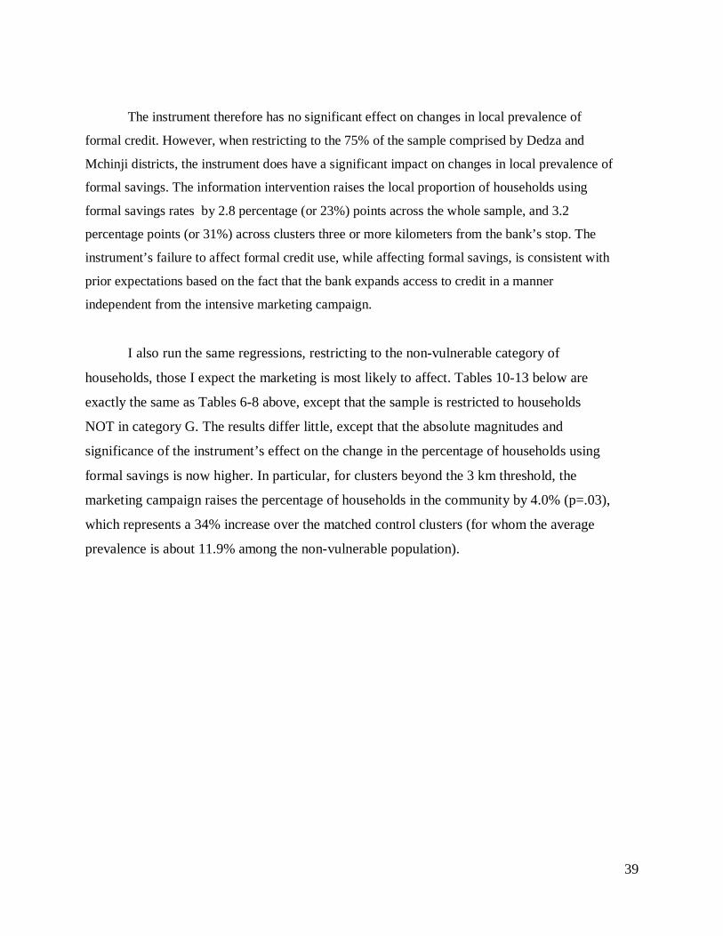
39

The instrument therefore has no significant effect on changes in local prevalence of

formal credit. However, when restricting to the 75% of the sample comprised by Dedza and

Mchinji districts, the instrument does have a significant impact on changes in local prevalence of

formal savings. The information intervention raises the local proportion of households using

formal savings rates by 2.8 percentage (or 23%) points across the whole sample, and 3.2

percentage points (or 31%) across clusters three or more kilometers from the bank’s stop. The

instrument’s failure to affect formal credit use, while affecting formal savings, is consistent with

prior expectations based on the fact that the bank expands access to credit in a manner

independent from the intensive marketing campaign.

I also run the same regressions, restricting to the non-vulnerable category of

households, those I expect the marketing is most likely to affect. Tables 10-13 below are

exactly the same as Tables 6-8 above, except that the sample is restricted to households

NOT in category G. The results differ little, except that the absolute magnitudes and

significance of the instrument’s effect on the change in the percentage of households using

formal savings is now higher. In particular, for clusters beyond the 3 km threshold, the

marketing campaign raises the percentage of households in the community by 4.0% (p=.03),

which represents a 34% increase over the matched control clusters (for whom the average

prevalence is about 11.9% among the non-vulnerable population).

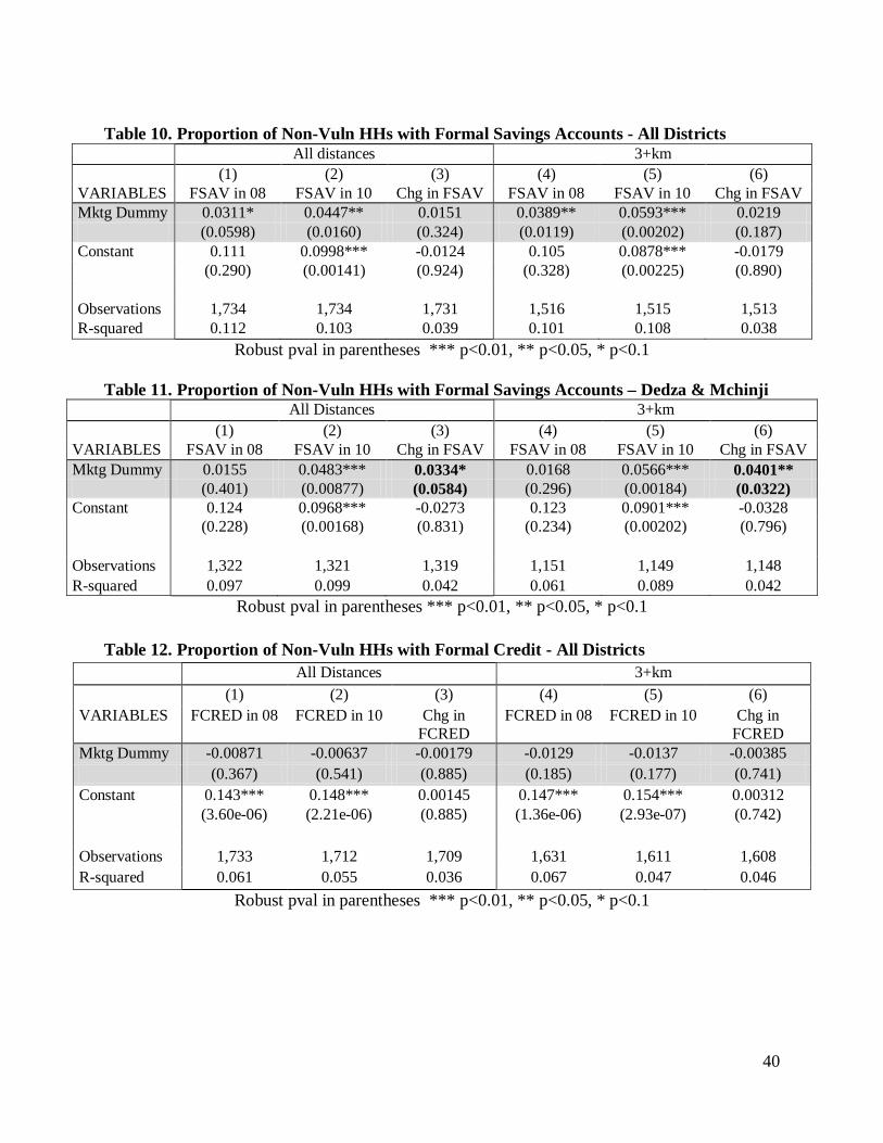
40

Table 10. Proportion of Non-Vuln HHs with Formal Savings Accounts - All Districts

All distances 3+km (1) (2) (3) (4) (5) (6) VARIABLES FSAV in 08 FSAV in 10 Chg in FSAV FSAV in 08 FSAV in 10 Chg in FSAV Mktg Dummy 0.0311* 0.0447** 0.0151 0.0389** 0.0593*** 0.0219 (0.0598) (0.0160) (0.324) (0.0119) (0.00202) (0.187) Constant 0.111 0.0998*** -0.0124 0.105 0.0878*** -0.0179 (0.290) (0.00141) (0.924) (0.328) (0.00225) (0.890) Observations 1,734 1,734 1,731 1,516 1,515 1,513 R-squared 0.112 0.103 0.039 0.101 0.108 0.038

Robust pval in parentheses *** p<0.01, ** p<0.05, * p<0.1

Table 11. Proportion of Non-Vuln HHs with Formal Savings Accounts – Dedza & Mchinji All Distances 3+km (1) (2) (3) (4) (5) (6) VARIABLES FSAV in 08 FSAV in 10 Chg in FSAV FSAV in 08 FSAV in 10 Chg in FSAV Mktg Dummy 0.0155 0.0483*** 0.0334* 0.0168 0.0566*** 0.0401** (0.401) (0.00877) (0.0584) (0.296) (0.00184) (0.0322) Constant 0.124 0.0968*** -0.0273 0.123 0.0901*** -0.0328 (0.228) (0.00168) (0.831) (0.234) (0.00202) (0.796) Observations 1,322 1,321 1,319 1,151 1,149 1,148 R-squared 0.097 0.099 0.042 0.061 0.089 0.042

Robust pval in parentheses *** p<0.01, ** p<0.05, * p<0.1 Table 12. Proportion of Non-Vuln HHs with Formal Credit - All Districts

All Distances 3+km (1) (2) (3) (4) (5) (6) VARIABLES FCRED in 08 FCRED in 10 Chg in

FCRED FCRED in 08 FCRED in 10 Chg in

FCRED Mktg Dummy -0.00871 -0.00637 -0.00179 -0.0129 -0.0137 -0.00385 (0.367) (0.541) (0.885) (0.185) (0.177) (0.741) Constant 0.143*** 0.148*** 0.00145 0.147*** 0.154*** 0.00312 (3.60e-06) (2.21e-06) (0.885) (1.36e-06) (2.93e-07) (0.742) Observations 1,733 1,712 1,709 1,631 1,611 1,608 R-squared 0.061 0.055 0.036 0.067 0.047 0.046

Robust pval in parentheses *** p<0.01, ** p<0.05, * p<0.1

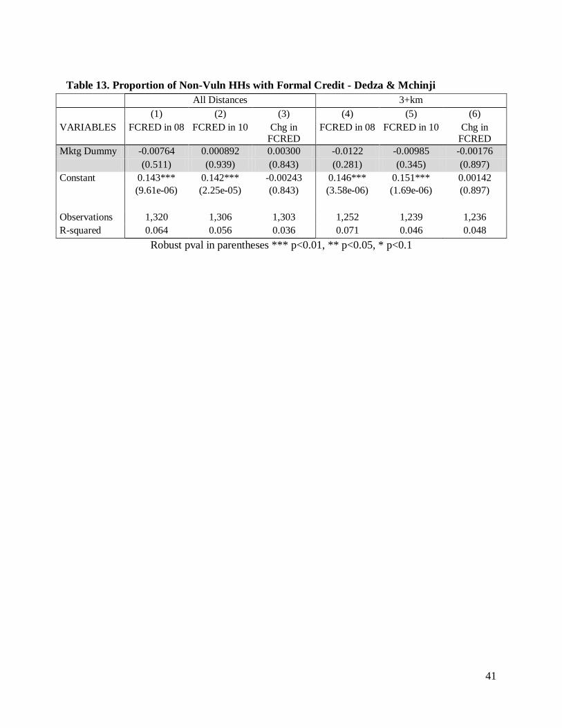
41

Table 13. Proportion of Non-Vuln HHs with Formal Credit - Dedza & Mchinji

All Distances 3+km (1) (2) (3) (4) (5) (6) VARIABLES FCRED in 08 FCRED in 10 Chg in

FCRED FCRED in 08 FCRED in 10 Chg in

FCRED Mktg Dummy -0.00764 0.000892 0.00300 -0.0122 -0.00985 -0.00176 (0.511) (0.939) (0.843) (0.281) (0.345) (0.897) Constant 0.143*** 0.142*** -0.00243 0.146*** 0.151*** 0.00142 (9.61e-06) (2.25e-05) (0.843) (3.58e-06) (1.69e-06) (0.897) Observations 1,320 1,306 1,303 1,252 1,239 1,236 R-squared 0.064 0.056 0.036 0.071 0.046 0.048

Robust pval in parentheses *** p<0.01, ** p<0.05, * p<0.1

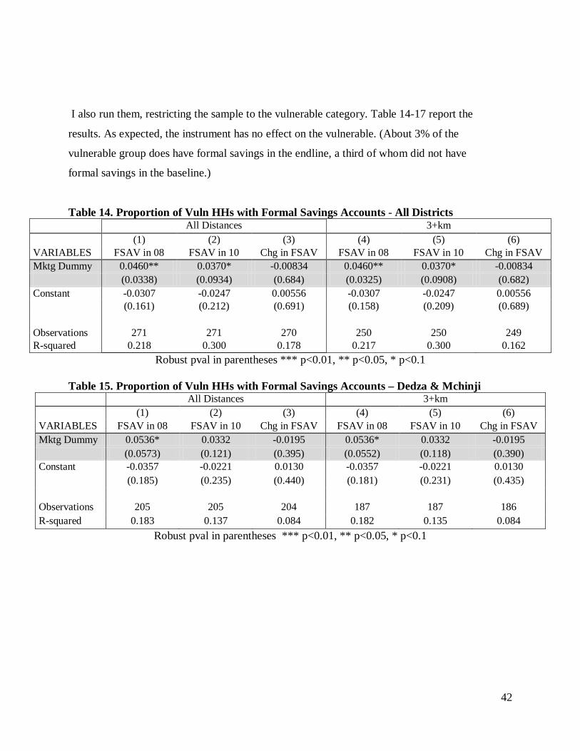
42

I also run them, restricting the sample to the vulnerable category. Table 14-17 report the

results. As expected, the instrument has no effect on the vulnerable. (About 3% of the

vulnerable group does have formal savings in the endline, a third of whom did not have

formal savings in the baseline.)

Table 14. Proportion of Vuln HHs with Formal Savings Accounts - All Districts All Distances 3+km (1) (2) (3) (4) (5) (6) VARIABLES FSAV in 08 FSAV in 10 Chg in FSAV FSAV in 08 FSAV in 10 Chg in FSAV Mktg Dummy 0.0460** 0.0370* -0.00834 0.0460** 0.0370* -0.00834 (0.0338) (0.0934) (0.684) (0.0325) (0.0908) (0.682) Constant -0.0307 -0.0247 0.00556 -0.0307 -0.0247 0.00556 (0.161) (0.212) (0.691) (0.158) (0.209) (0.689) Observations 271 271 270 250 250 249 R-squared 0.218 0.300 0.178 0.217 0.300 0.162

Robust pval in parentheses *** p<0.01, ** p<0.05, * p<0.1 Table 15. Proportion of Vuln HHs with Formal Savings Accounts – Dedza & Mchinji

All Distances 3+km (1) (2) (3) (4) (5) (6) VARIABLES FSAV in 08 FSAV in 10 Chg in FSAV FSAV in 08 FSAV in 10 Chg in FSAV Mktg Dummy 0.0536* 0.0332 -0.0195 0.0536* 0.0332 -0.0195 (0.0573) (0.121) (0.395) (0.0552) (0.118) (0.390) Constant -0.0357 -0.0221 0.0130 -0.0357 -0.0221 0.0130 (0.185) (0.235) (0.440) (0.181) (0.231) (0.435) Observations 205 205 204 187 187 186 R-squared 0.183 0.137 0.084 0.182 0.135 0.084

Robust pval in parentheses *** p<0.01, ** p<0.05, * p<0.1

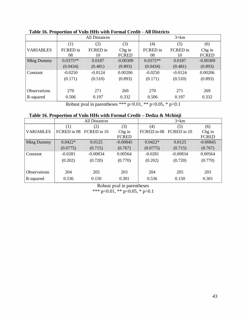
43

Table 16. Proportion of Vuln HHs with Formal Credit - All Districts All Distances 3+km (1) (2) (3) (4) (5) (6) VARIABLES FCRED in

08 FCRED in

10 Chg in

FCRED FCRED in

08 FCRED in

10 Chg in

FCRED Mktg Dummy 0.0375** 0.0187 -0.00309 0.0375** 0.0187 -0.00309 (0.0434) (0.481) (0.893) (0.0434) (0.481) (0.893) Constant -0.0250 -0.0124 0.00206 -0.0250 -0.0124 0.00206 (0.171) (0.510) (0.893) (0.171) (0.510) (0.893) Observations 270 271 269 270 271 269 R-squared 0.506 0.197 0.332 0.506 0.197 0.332

Robust pval in parentheses *** p<0.01, ** p<0.05, * p<0.1 Table 16. Proportion of Vuln HHs with Formal Credit – Dedza & Mchinji

All Distances 3+km (1) (2) (3) (4) (5) (6) VARIABLES FCRED in 08 FCRED in 10 Chg in

FCRED FCRED in 08 FCRED in 10 Chg in

FCRED Mktg Dummy 0.0422* 0.0125 -0.00845 0.0422* 0.0125 -0.00845 (0.0775) (0.715) (0.767) (0.0775) (0.715) (0.767) Constant -0.0281 -0.00834 0.00564 -0.0281 -0.00834 0.00564 (0.202) (0.720) (0.770) (0.202) (0.720) (0.770) Observations 204 205 203 204 205 203 R-squared 0.536 0.150 0.301 0.536 0.150 0.301

Robust pval in parentheses *** p<0.01, ** p<0.05, * p<0.1

44

6. IIT: The Link Between the Instrument & Receipts of Assistance

While the conceptual framework for understanding how savings account adoption may

affect inter-household transfers began with an analysis of account-adopters’ behavior, the

empirical analysis focuses primarily on the effects of local formal savings adoption on receipts

of assistance, particularly by non-adopting vulnerable households. This indirect approach to

testing the model’s hypotheses is in part a response to the empirical challenge presented by the

data. Most communities are likely to have relatively few “wealthy” households (who are more

likely to be initial service-adopters), and it is reasonable to suppose that when wealthier

households provide assistance, they give to multiple households. A random sample from this

environment is therefore likely to have many more households that are potential supplicants (or

assistance recipients) than households that are account-adopters. This means that tests on the

behavior of adopting households are likely to lack statistical power. Focusing on assistance

receipts (rather than gifts-out) also places the analysis squarely on one of the most sensitive

issues for poverty policy: whether and how formal savings expansion affects non-users, and in

particular, the most vulnerable members of the community.

Discussion of the impacts of formal savings expansion begins with a brief look at simple

percentage changes across the encouraged and non-encouraged clusters. It then proceeds to

analysis of a variety of sharp differences in vulnerable-household transfer receipts, between

marketing and non-marketing village clusters. In the context of assessing direct impacts, this

would be analogous to intention to treat (ITT) effects. However, since analyzing indirect effects,

I call this the “indirect intention to treat”, or “IIT”. The indirect intention to treat effects are

interpreted as preliminary evidence suggesting a causal effect from savings accounts.

While the baseline includes data on a broad range of financial services and transactions,

I was only able to add the detailed questions on inter-household transfers to the endline survey.

Discussion of the impacts of formal savings adoption on inter-household gifts therefore begins

with a cross-sectional analysis of the endline data.

45

As long as the marketing inducement is randomly assigned, it is valid to interpret

relationships between marketing and household outcomes as causal. However, the full panel

does contain limited information on certain types of wealth transfers that are similar to the gifts-

information captured only in the endline. I therefore follow the cross-sectional analysis with a

difference-in-differences analysis of these related types of transfers. The results of this panel

analysis are important in their own right. However, they also provide strong evidence that the

endline patterns in cash-gifts were not present in the baseline, but were instead caused by the

marketing-induced spike in the number of new savers in the community.

A First Glance It is worth a quick look at the differences in cash-gift receipts by marketing and non-

marketing clusters. We gathered data on cash gifts of 50 kwacha (about $.30) or more,

received over a 90-day recall period preceding the interview.27 The vast majority are from

within the local community. While we did not gather data on the actual distances between

giving and receiving households, nor on whether the households were located in the same

village, the data do include total round-trip travel times required to obtain each gift. About

80% of the reported round-trip travel times are below 30 minutes (implying one-way trips of

a maximum 5-15 minutes)28

Table 3 shows simple comparisons of the percentage of households receiving cash

gifts in the non-marketing and marketing clusters – overall and by household vulnerability

type. Appendix Table A1 is analogous, but compares percentages of households receiving

multiple cash gifts. Before analyzing separately by vulnerability level, we already see a large

. This proportion remains about 80% whether looking at the

sample overall, or just the highly vulnerable category. Given that the standard mode of

transport in these areas is usually walking, and sometimes bicycling, this suggests that most

of these transfers are between households within the same village, or at furthest from

neighboring villages.

27 Interviewers were intensively trained on the difference between a “gift” and a loan, the latter carrying with it an expectation of repayment of some type of wealth in the future. In addition, the module I added to the survey with questions on gifts came after a section in which detailed information was already gathered on loans. Interviewers were trained to distinguish between the two and collect information on each only in their respective parts of the questionnaire. 28 The question was asked so as to include time spent at the location of where they were requesting or receiving the gift. That is, it is a total time-cost figure, inclusive of time spent communicating with anyone providing assistance.

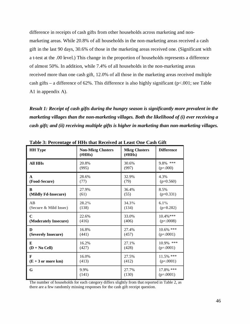
46

difference in receipts of cash gifts from other households across marketing and non-

marketing areas. While 20.8% of all households in the non-marketing areas received a cash

gift in the last 90 days, 30.6% of those in the marketing areas received one. (Significant with

a t-test at the .00 level.) This change in the proportion of households represents a difference

of almost 50%. In addition, while 7.4% of all households in the non-marketing areas

received more than one cash gift, 12.0% of all those in the marketing areas received multiple

cash gifts – a difference of 62%. This difference is also highly significant (p<.001; see Table

A1 in appendix A).

Result 1: Receipt of cash gifts during the hungry season is significantly more prevalent in the

marketing villages than the non-marketing villages. Both the likelihood of (i) ever receiving a

cash gift; and (ii) receiving multiple gifts is higher in marketing than non-marketing villages.

Table 3: Percentage of HHs that Received at Least One Cash Gift HH Type Non-Mktg Clusters

(#HHs) Mktg Clusters (#HHs)

Difference

All HHs 20.8% (995)

30.6% (997)

9.8% *** (p=.000)

A (Food-Secure)

28.6% (77)

32.9% (79)

4.3% (p=0.560)

B (Mildly Fd-Insecure)

27.9% (61)

36.4% (55)

8.5% (p=0.331)

AB (Secure & Mild Insec)

28.2% (138)

34.3% (134)

6.1% (p=0.282)

C (Moderately Insecure)

22.6% (416)

33.0% (406)

10.4%*** (p=.0008)

D (Severely Insecure)

16.8% (441)

27.4% (457)

10.6% *** (p=.0001)

E (D + No Cell)

16.2% (427)

27.1% (428)

10.9% *** (p=.0001)

F (E + 3 or more km)

16.0% (413)

27.5% (412)

11.5% *** (p=.0001)

G 9.9% (141)

27.7% (130)

17.8% *** (p=.0001)

The number of households for each category differs slightly from that reported in Table 2, as there are a few randomly missing responses for the cash gift receipt question.

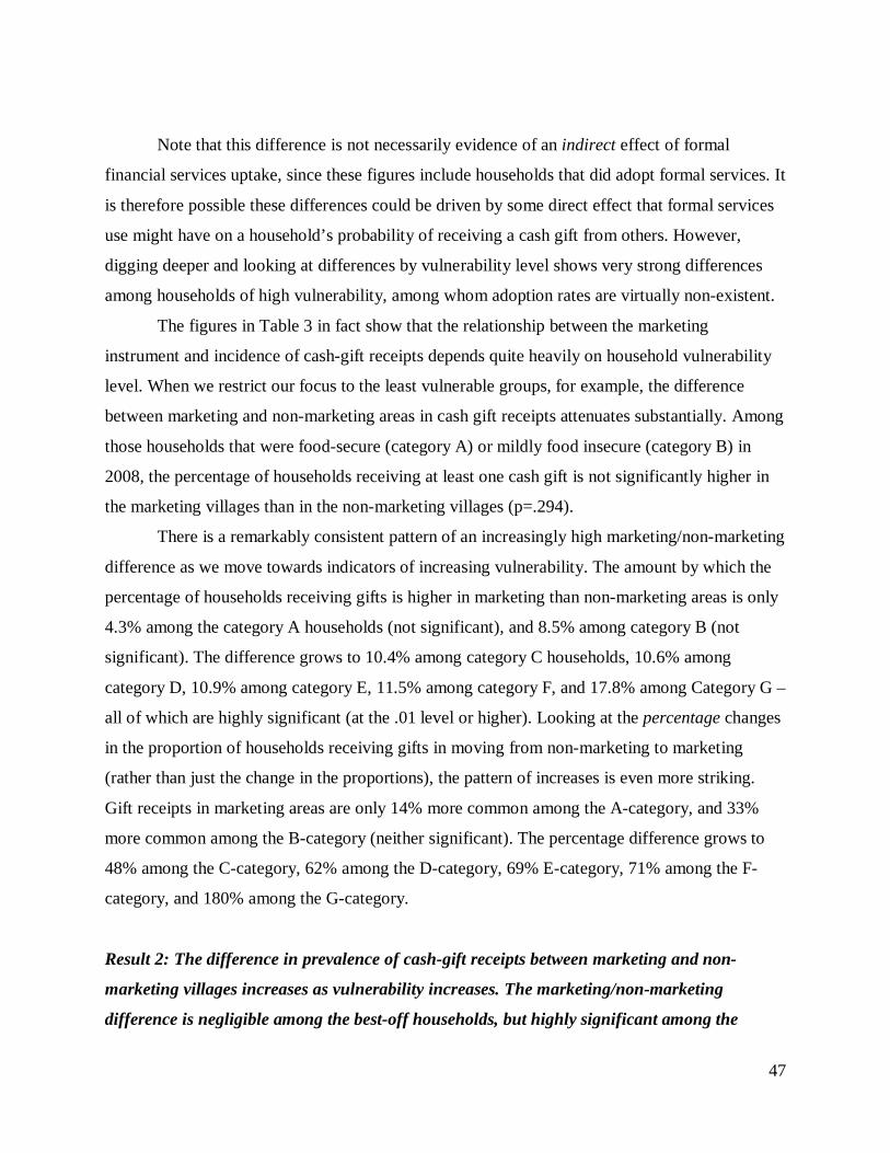
47

Note that this difference is not necessarily evidence of an indirect effect of formal

financial services uptake, since these figures include households that did adopt formal services. It

is therefore possible these differences could be driven by some direct effect that formal services

use might have on a household’s probability of receiving a cash gift from others. However,

digging deeper and looking at differences by vulnerability level shows very strong differences

among households of high vulnerability, among whom adoption rates are virtually non-existent.

The figures in Table 3 in fact show that the relationship between the marketing

instrument and incidence of cash-gift receipts depends quite heavily on household vulnerability

level. When we restrict our focus to the least vulnerable groups, for example, the difference

between marketing and non-marketing areas in cash gift receipts attenuates substantially. Among

those households that were food-secure (category A) or mildly food insecure (category B) in

2008, the percentage of households receiving at least one cash gift is not significantly higher in

the marketing villages than in the non-marketing villages (p=.294).

There is a remarkably consistent pattern of an increasingly high marketing/non-marketing

difference as we move towards indicators of increasing vulnerability. The amount by which the

percentage of households receiving gifts is higher in marketing than non-marketing areas is only

4.3% among the category A households (not significant), and 8.5% among category B (not

significant). The difference grows to 10.4% among category C households, 10.6% among

category D, 10.9% among category E, 11.5% among category F, and 17.8% among Category G –

all of which are highly significant (at the .01 level or higher). Looking at the percentage changes

in the proportion of households receiving gifts in moving from non-marketing to marketing

(rather than just the change in the proportions), the pattern of increases is even more striking.

Gift receipts in marketing areas are only 14% more common among the A-category, and 33%

more common among the B-category (neither significant). The percentage difference grows to

48% among the C-category, 62% among the D-category, 69% E-category, 71% among the F-

category, and 180% among the G-category.

Result 2: The difference in prevalence of cash-gift receipts between marketing and non-

marketing villages increases as vulnerability increases. The marketing/non-marketing

difference is negligible among the best-off households, but highly significant among the

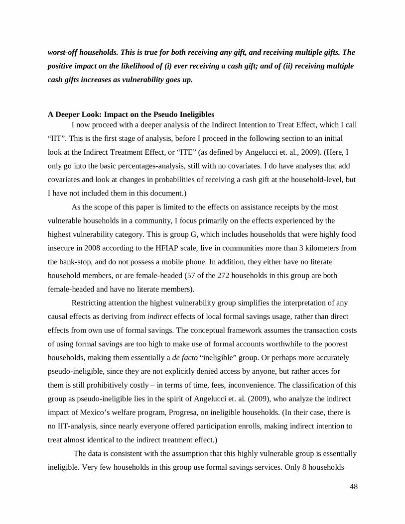
48

worst-off households. This is true for both receiving any gift, and receiving multiple gifts. The

positive impact on the likelihood of (i) ever receiving a cash gift; and of (ii) receiving multiple

cash gifts increases as vulnerability goes up.

A Deeper Look: Impact on the Pseudo Ineligibles

I now proceed with a deeper analysis of the Indirect Intention to Treat Effect, which I call

“IIT”. This is the first stage of analysis, before I proceed in the following section to an initial

look at the Indirect Treatment Effect, or “ITE” (as defined by Angelucci et. al., 2009). (Here, I

only go into the basic percentages-analysis, still with no covariates. I do have analyses that add

covariates and look at changes in probabilities of receiving a cash gift at the household-level, but

I have not included them in this document.)

As the scope of this paper is limited to the effects on assistance receipts by the most

vulnerable households in a community, I focus primarily on the effects experienced by the

highest vulnerability category. This is group G, which includes households that were highly food

insecure in 2008 according to the HFIAP scale, live in communities more than 3 kilometers from

the bank-stop, and do not possess a mobile phone. In addition, they either have no literate

household members, or are female-headed (57 of the 272 households in this group are both

female-headed and have no literate members).

Restricting attention the highest vulnerability group simplifies the interpretation of any

causal effects as deriving from indirect effects of local formal savings usage, rather than direct

effects from own use of formal savings. The conceptual framework assumes the transaction costs

of using formal savings are too high to make use of formal accounts worthwhile to the poorest

households, making them essentially a de facto “ineligible” group. Or perhaps more accurately

pseudo-ineligible, since they are not explicitly denied access by anyone, but rather acces for

them is still prohibitively costly – in terms of time, fees, inconvenience. The classification of this

group as pseudo-ineligible lies in the spirit of Angelucci et. al. (2009), who analyze the indirect

impact of Mexico’s welfare program, Progresa, on ineligible households. (In their case, there is

no IIT-analysis, since nearly everyone offered participation enrolls, making indirect intention to

treat almost identical to the indirect treatment effect.)

The data is consistent with the assumption that this highly vulnerable group is essentially

ineligible. Very few households in this group use formal savings services. Only 8 households

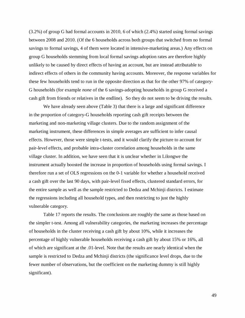
49

(3.2%) of group G had formal accounts in 2010, 6 of which (2.4%) started using formal savings

between 2008 and 2010. (Of the 6 households across both groups that switched from no formal

savings to formal savings, 4 of them were located in intensive-marketing areas.) Any effects on

group G households stemming from local formal savings adoption rates are therefore highly

unlikely to be caused by direct effects of having an account, but are instead attributable to

indirect effects of others in the community having accounts. Moreover, the response variables for

these few households tend to run in the opposite direction as that for the other 97% of category-

G households (for example none of the 6 savings-adopting households in group G received a

cash gift from friends or relatives in the endline). So they do not seem to be driving the results.

We have already seen above (Table 3) that there is a large and significant difference

in the proportion of category-G households reporting cash gift receipts between the

marketing and non-marketing village clusters. Due to the random assignment of the

marketing instrument, these differences in simple averages are sufficient to infer causal

effects. However, those were simple t-tests, and it would clarify the picture to account for

pair-level effects, and probable intra-cluster correlation among households in the same

village cluster. In addition, we have seen that it is unclear whether in Lilongwe the

instrument actually boosted the increase in proportion of households using formal savings. I

therefore run a set of OLS regressions on the 0-1 variable for whether a household received

a cash gift over the last 90 days, with pair-level fixed effects, clustered standard errors, for

the entire sample as well as the sample restricted to Dedza and Mchinji districts. I estimate

the regressions including all household types, and then restricting to just the highly

vulnerable category.

Table 17 reports the results. The conclusions are roughly the same as those based on

the simpler t-test. Among all vulnerability categories, the marketing increases the percentage

of households in the cluster receiving a cash gift by about 10%, while it increases the

percentage of highly vulnerable households receiving a cash gift by about 15% or 16%, all

of which are significant at the .01-level. Note that the results are nearly identical when the

sample is restricted to Dedza and Mchinji districts (the significance level drops, due to the

fewer number of observations, but the coefficient on the marketing dummy is still highly

significant).

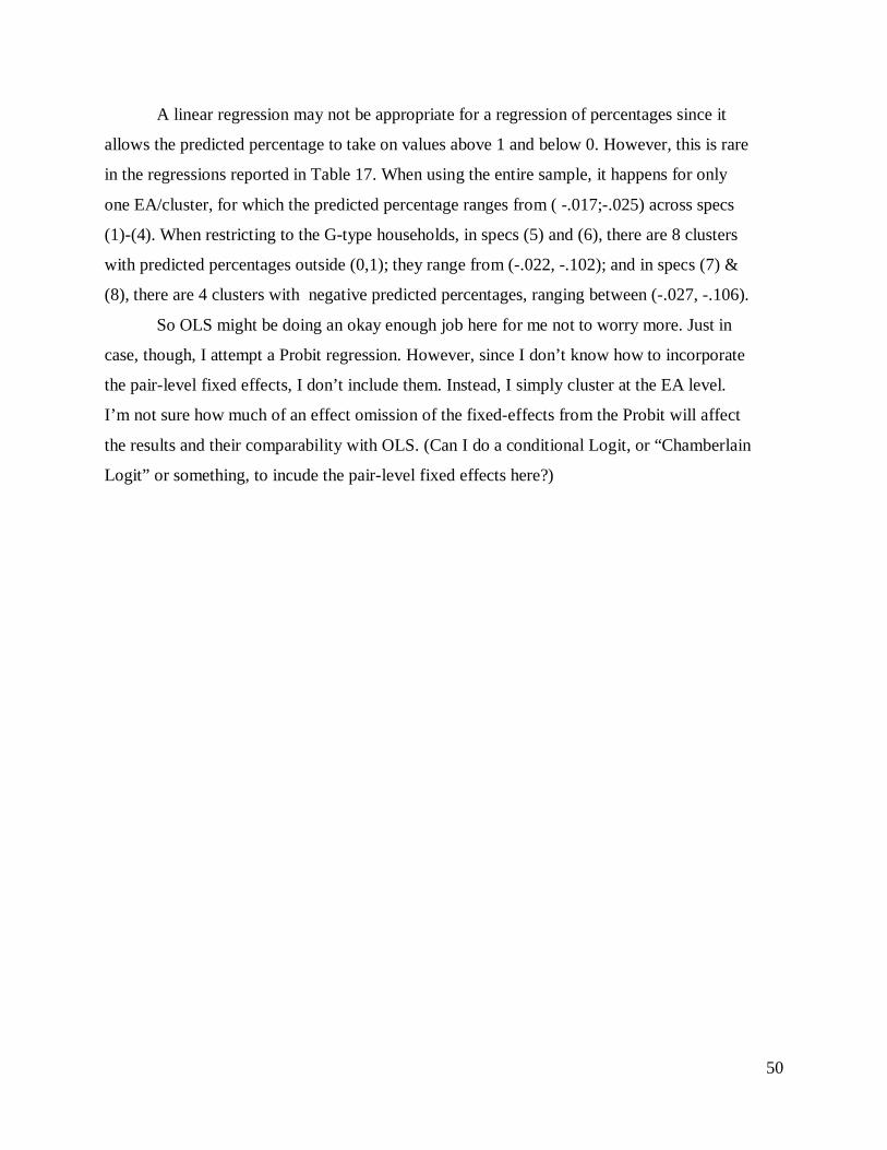
50

A linear regression may not be appropriate for a regression of percentages since it

allows the predicted percentage to take on values above 1 and below 0. However, this is rare

in the regressions reported in Table 17. When using the entire sample, it happens for only

one EA/cluster, for which the predicted percentage ranges from ( -.017;-.025) across specs

(1)-(4). When restricting to the G-type households, in specs (5) and (6), there are 8 clusters

with predicted percentages outside (0,1); they range from (-.022, -.102); and in specs (7) &

(8), there are 4 clusters with negative predicted percentages, ranging between (-.027, -.106).

So OLS might be doing an okay enough job here for me not to worry more. Just in

case, though, I attempt a Probit regression. However, since I don’t know how to incorporate

the pair-level fixed effects, I don’t include them. Instead, I simply cluster at the EA level.

I’m not sure how much of an effect omission of the fixed-effects from the Probit will affect

the results and their comparability with OLS. (Can I do a conditional Logit, or “Chamberlain

Logit” or something, to incude the pair-level fixed effects here?)

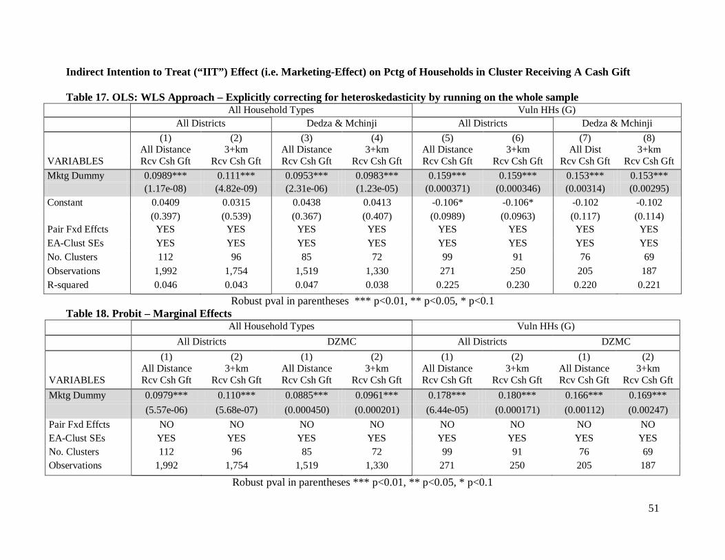
51

Indirect Intention to Treat (“IIT”) Effect (i.e. Marketing-Effect) on Pctg of Households in Cluster Receiving A Cash Gift Table 17. OLS: WLS Approach – Explicitly correcting for heteroskedasticity by running on the whole sample

All Household Types Vuln HHs (G) All Districts Dedza & Mchinji All Districts Dedza & Mchinji (1)

All Distance (2)

3+km (3)

All Distance (4)

3+km (5)

All Distance (6)

3+km (7)

All Dist (8)

3+km VARIABLES Rcv Csh Gft Rcv Csh Gft Rcv Csh Gft Rcv Csh Gft Rcv Csh Gft Rcv Csh Gft Rcv Csh Gft Rcv Csh Gft Mktg Dummy 0.0989*** 0.111*** 0.0953*** 0.0983*** 0.159*** 0.159*** 0.153*** 0.153*** (1.17e-08) (4.82e-09) (2.31e-06) (1.23e-05) (0.000371) (0.000346) (0.00314) (0.00295) Constant 0.0409 0.0315 0.0438 0.0413 -0.106* -0.106* -0.102 -0.102 (0.397) (0.539) (0.367) (0.407) (0.0989) (0.0963) (0.117) (0.114) Pair Fxd Effcts YES YES YES YES YES YES YES YES EA-Clust SEs YES YES YES YES YES YES YES YES No. Clusters 112 96 85 72 99 91 76 69 Observations 1,992 1,754 1,519 1,330 271 250 205 187 R-squared 0.046 0.043 0.047 0.038 0.225 0.230 0.220 0.221

Robust pval in parentheses *** p<0.01, ** p<0.05, * p<0.1 Table 18. Probit – Marginal Effects

All Household Types Vuln HHs (G) All Districts DZMC All Districts DZMC (1)

All Distance (2)

3+km (1)

All Distance (2)

3+km (1)

All Distance (2)

3+km (1)

All Distance (2)

3+km VARIABLES Rcv Csh Gft Rcv Csh Gft Rcv Csh Gft Rcv Csh Gft Rcv Csh Gft Rcv Csh Gft Rcv Csh Gft Rcv Csh Gft Mktg Dummy 0.0979*** 0.110*** 0.0885*** 0.0961*** 0.178*** 0.180*** 0.166*** 0.169*** (5.57e-06) (5.68e-07) (0.000450) (0.000201) (6.44e-05) (0.000171) (0.00112) (0.00247) Pair Fxd Effcts NO NO NO NO NO NO NO NO EA-Clust SEs YES YES YES YES YES YES YES YES No. Clusters 112 96 85 72 99 91 76 69 Observations 1,992 1,754 1,519 1,330 271 250 205 187

Robust pval in parentheses *** p<0.01, ** p<0.05, * p<0.1

52

I repeat the same IIT analysis as above, but in a manner that, though inferior, is directly

comparable to the ITE analysis that follows. Instead using village-cluster as the unit of

observation (rather than household), and using aggregated variables from the cluster-level as the

independent and dependent variables. That is, the left-hand side variable is simply the percentage

of households within each cluster that received a cash gift (for columns 1-4), or the percentage of

type-G households in each cluster that received a cash gift (for columns 5-8). The only difference

here is that I am regressing the actual percentage here, rather than the household-level 0/1

variable. (That is, I first calculate for each cluster the mean value for the 0-1 household indicator

for receipt of cash gift, then regress that on the marketing dummy for that village cluster).

The point estimates should be exactly the same through this approach as through the

approach where I use the household as the unit of observation. The only econometric difference

is that I am using heteroskedasticity-robust sandwich errors to estimated the standard errors,

instead of FGLS – i.e. weighting each cluster-observation by the number of observations they

contribute (which is more efficient). The reason I show these tables here is that I am constrained

to use this approach in the instrumentable variables regressions for ITE further below, since I

don’t know how to implement the FGLS-approach.

Table 19 reports the results. Interestingly, the point estimates are different. This shouldn’t

have happened, I don’t think. I’m not sure what’s going on here. In any case, they are close to

the effects reported in Table 17. The main difference is that the significance has dropped, so that

the IIT impact of the marketing on percentage of vulnerable households receiving cash gifts is

now significant at the .05-level. In addition, the predicted percentages violate the (0,1) bounds

even more rarely than for the FGLS approach above. (Just one EA when using the full sample,

ranging from -2% to -2.7%; and only 1 or 2 EAs when using the type-G sample (one EA usually

at about -0.7%, the other ranging between -7.85% and -9.0%, depending on the spec. ). A Probit

would not make sense in the context of using the means from each EA (since it’s not a 0/1

variable, but rather a continuous variable -- it’s the percentage). So I do not compare OLS to a

model that would force predicted outcomes to remain in the (0,1) range.

I think I should also be able to do this with random effects instead, in order to get even

tighter bounds on the parameter estimates, since the pair-effect is not correlated with treatment

status, and I don’t need to cluster at village-cluster level because each observation is at the

53

cluster level.

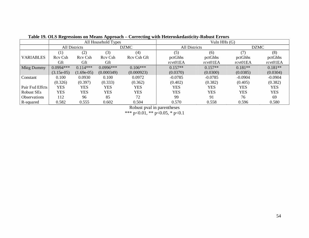
54

Table 19. OLS Regressions on Means Approach – Correcting with Heteroskedasticity-Robust Errors

All Household Types Vuln HHs (G) All Districts DZMC All Districts DZMC (1) (2) (3) (4) (5) (6) (7) (8) VARIABLES Rcv Csh

Gft Rcv Csh

Gft Rcv Csh

Gft Rcv Csh Gft pctGhhs

rcvt01EA pctGhhs

rcvt01EA pctGhhs

rcvt01EA pctGhhs

rcvt01EA Mktg Dummy 0.0994*** 0.114*** 0.0996*** 0.106*** 0.157** 0.157** 0.181** 0.181** (3.15e-05) (1.69e-05) (0.000349) (0.000923) (0.0370) (0.0300) (0.0385) (0.0304) Constant 0.100 0.0930 0.100 0.0972 -0.0785 -0.0785 -0.0904 -0.0904 (0.326) (0.397) (0.333) (0.362) (0.402) (0.382) (0.405) (0.382) Pair Fxd Effcts YES YES YES YES YES YES YES YES Robust SEs YES YES YES YES YES YES YES YES Observations 112 96 85 72 99 91 76 69 R-squared 0.582 0.555 0.602 0.504 0.570 0.558 0.596 0.580

Robust pval in parentheses *** p<0.01, ** p<0.05, * p<0.1

55

Cash Gift Amounts Received

I also analyze whether cash gift amounts received by vulnerable households appear to be

affected by formal savings adoption rates in the local community. I don’t show the results in this

version, for the sake of brevity. I analyze the most recent gift amount (we only gather amount for

the most recent gift over the last 90 days and the largest gift over the last 90 days) and find that,

conditional on receiving a cash gift, cash gift amounts do not change. That is, when I restrict the

sample to those households that report receiving a cash gift and regress the amount of the gift on

the marketing dummy, the dummy is not significant. This is true for both the full sample (for

which number of households receiving gifts is n=512, and the p-value for the significance of

marketing dummy is p=.188), and for the sample of just the vulnerable households (cash gift-

receivers number is n=50, p=.214).

If I run a Tobit, with censoring from below at 50 kwacha, the coefficient on the

marketing dummy is highly significant – overall, or restricting to just the vulnerable households.

But I think this is simply driven by the probability of receiving a cash gift at all (right?).

The results suggest that the key decision of a benefactor household is not how much to

give in a cash gift to a supplicant, but instead whether to give a cash gift at all. This may indicate

that the gifts serve a similar purpose, one with a stable or commonly understood cost – for

example, small amounts of emergency food-consumption maintenance.

Result 3: The instrument for formal savings adoption is not associated with an increase in the

value of cash-gifts received, but instead only the probability of receipt.

In-Kind Gifts & Payment of Fees

The data also include information on receipts of in-kind gifts, as well as someone making

payment to a third party on behalf of a household member (e.g. paying for a household member’s

medical fees, school fees, etc.). Just as for the cash-gift variable, the question is limited to a

recall period of 90 days, and restricts amounts to 50 kwacha (approx. $0.30) and above.

56

Appendix __Q__ shows the results from an IIT analysis of these transfer receipts which parallels

that for cash-gifts.

Though the estimated effects are rarely significant, the signs are consistent with the

results for cash gifts. In particular, the percentage of highly vulnerable households receiving help

paying third party fees is 4.4 percentage points higher in communities that received the

information intervention, representing a 62% difference (p=.208 with a two-sided t-test). The

percentage of highly vulnerable households that report an in-kind gift is 8.3 percentage points

higher in information-treated communities, representing a 33% difference (p=.138, with a two-

sided t-test).

This suggests on the one hand that direct monetary transfers to households are more

sensitive to the change introduced by formal savings uptake that non-monetary wealth transfers,

or monetary payments to a third party. More importantly, it suggests that the cash-gifts result is

not simply a substitution effect. It is not the case, for example, that vulnerable households are

now receiving cash gifts in lieu of in-kind gifts, such as food. This is important, as it more

strongly suggests an improvement in welfares of the vulnerable households, an issue that will be

taken up in greater detail in section 8(?)

Result 4: The result does not appear to be driven by a substitution of cash-assistance for other

types of assistance. This suggests a positive welfare effect by recipients is probable.

Panel Analysis: Impact of Information Intervention on Informal Loans Received

Since the marketing encouragement was randomly assigned, cross-sectional

estimates of the effect of marketing-induced increases in local savings account usage should

be consistent. That is, the randomization should ensure the pattern of differences in gift

receipts in the endline was not present in the baseline, nor derive from any systematic

differences between marketing and non-marketing clusters along any dimensions other than

the marketing campaign itself. Unfortunately, since there is no baseline data on gifts, this is

impossible to verify. The data do contain, however, data on informal loans received in both

years. The following panel analysis of two-year changes in receipt of loans from other

households serve as a robustness check on the assumption of no baseline difference. In this

57

capacity, they confirm causal interpretation of the cross-sectional results on cash-gifts. They

also stand as important results in their own right, given the extensive literature documenting

the importance of informal loans in consumption-smoothing.

The data include information on loans received from friends or relatives anytime in

the past two years. These are cash loans, for which the purpose is not specified by the

respondent. If formal savings accounts makes it easier for households to share wealth via

cash assistance in order to help other households smooth consumption, we might expect to

see the effect in loan-receipts as well as gifts. More generally, we might expect changes in

receipt of loans to at least loosely track changes in receipt of pure gifts of cash.

The percentage of highly vulnerable households reporting informal loans over

previous 2 years in 2008 was 39.7% in the information-treated clusters and 42.6% in the

information control clusters (41.2% overall). In 2010, this percentage rose to 49.2% in the

treated clusters, and remained constant at 42.6% in the control clusters. When restricting to

clusters 3 km out, the trend grows even stronger. In 2008, while 38.5% of the highly

vulnerable in the marketing clusters report informal loans, 45.0% of those in the non-

marketing clusters report them. In 2010, however, the percentage in the marketing clusters

rises to 50.4% and that in the non-marketing clusters drops to 43.4%. None of these cross-

sectional differences are significant with two-sided t-tests at conventional levels, but they

are highly suggestive.

Analyzing the changes, adding controls, and controlling for intra-cluster correlation

sharpens the picture. Table 20 reports results from a simple first-differenced regression of

informal loan receipt on a dummy for information intervention, with the sample restricted to

the highly vulnerable households. All regressions include clustered standard errors, and four

different regressions are shown – one without fixed effects, one with fixed effects at district

level, one with fixed effects at zone-level, and one with fixed effects at the cluster-pair level.

While differencing the data removes any time-invariant local fixed effects (such as variation

in norms, tastes, or degree of integration into the modern economy), it does not account for

any possible interactions of period changes with local variables or changes which vary

across communities. On the one hand, an adverse shock experienced by all communities in

the sample could be better mitigated by households in a community with extensive extra-

village linkages, freeing households to give loans more easily than in a community with

58

fewer extra-village links. On the other hand, any region-specific or spatially covariate

shocks which occur over the two-year period (positive or negative) may affect the ability of

neighboring households to provide assistance differently in one area than another.

The response variable is the change in whether a given vulnerable household

received an informal loan over the two years preceding the interview date. It can therefore

take values of {-1,0,1}, which correspond to going from receiving at least one or more loans

to receiving none, experiencing no change, and going from receiving no informal loan to

receiving one or more. The interpretation of the coefficient for the information intervention

is therefore the effect of the marketing on the percentage of vulnerable households that

received an informal loan. Table 21 reports results from the same regressions, but restricted

to Dedza and Mchinji.

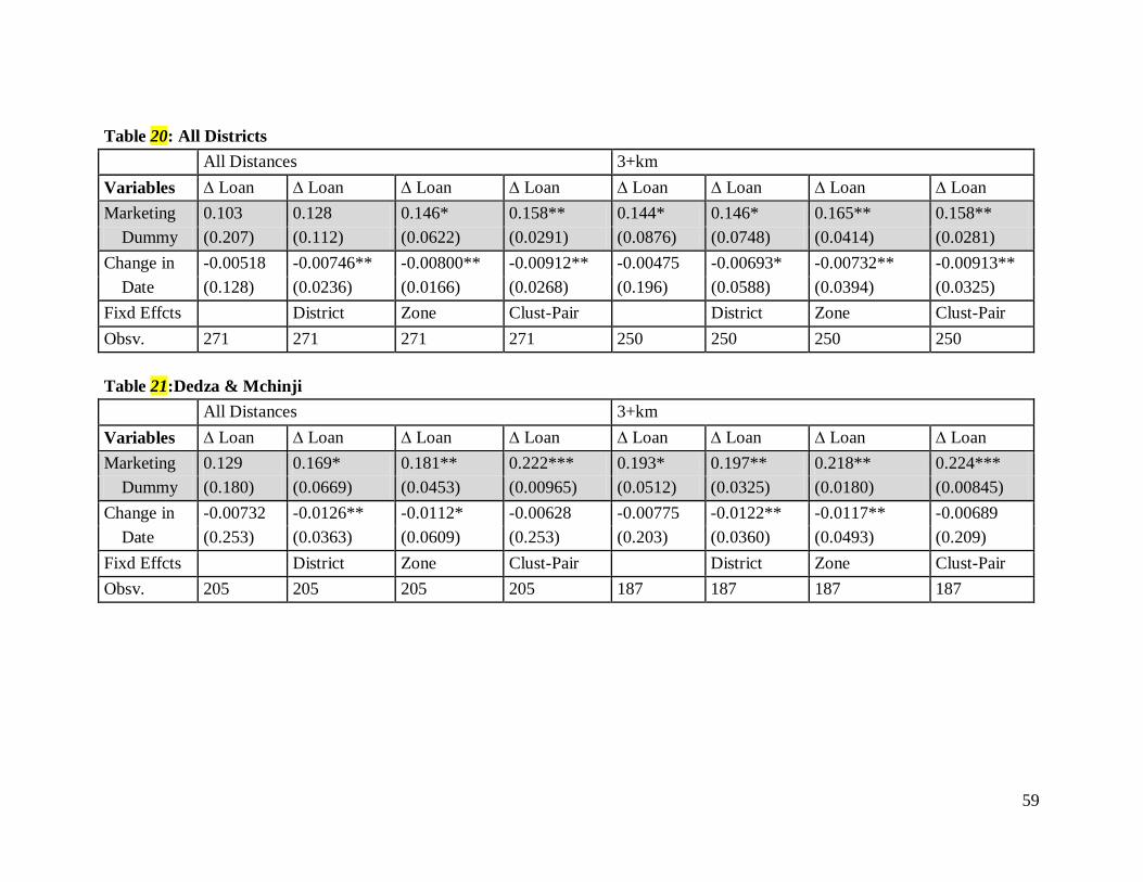
59

Table 20: All Districts All Distances 3+km Variables ∆ Loan ∆ Loan ∆ Loan ∆ Loan ∆ Loan ∆ Loan ∆ Loan ∆ Loan Marketing 0.103 0.128 0.146* 0.158** 0.144* 0.146* 0.165** 0.158** Dummy (0.207) (0.112) (0.0622) (0.0291) (0.0876) (0.0748) (0.0414) (0.0281) Change in -0.00518 -0.00746** -0.00800** -0.00912** -0.00475 -0.00693* -0.00732** -0.00913** Date (0.128) (0.0236) (0.0166) (0.0268) (0.196) (0.0588) (0.0394) (0.0325) Fixd Effcts District Zone Clust-Pair District Zone Clust-Pair Obsv. 271 271 271 271 250 250 250 250 Table 21:Dedza & Mchinji All Distances 3+km Variables ∆ Loan ∆ Loan ∆ Loan ∆ Loan ∆ Loan ∆ Loan ∆ Loan ∆ Loan Marketing 0.129 0.169* 0.181** 0.222*** 0.193* 0.197** 0.218** 0.224*** Dummy (0.180) (0.0669) (0.0453) (0.00965) (0.0512) (0.0325) (0.0180) (0.00845) Change in -0.00732 -0.0126** -0.0112* -0.00628 -0.00775 -0.0122** -0.0117** -0.00689 Date (0.253) (0.0363) (0.0609) (0.253) (0.203) (0.0360) (0.0493) (0.209) Fixd Effcts District Zone Clust-Pair District Zone Clust-Pair Obsv. 205 205 205 205 187 187 187 187

60

In all of the specifications, the estimated magnitudes are substantial, and they are

significant in most. They are always significant, and generally at high levels, when including

area fixed effects. In particular, when restricting to cluster pairs located three or more kilometers

from the nearest bank-stop, the effect is significant in all specifications, and raises the percentage

of vulnerable households receiving informal loans by an estimated 14.4 to 22.4 percentage points

after adjusting for intra-cluster correlation. The overall two-year change in percentage of highly

vulnerable receiving informal loans at the 3 km threshold is an increase of 4.8 percentage-points

(a drop of 1.6 percentage points in the information-control clusters, and an increase of 11.6

percentage points in the information-treated). The estimated effect is therefore substantial not

only in absolute but also relative terms.

Result 5: The instrument for local rates of formal savings adoption is associated with a

substantial increase in the two-year change in the proportion of highly vulnerable households

receiving cash-loans from friends or relatives.

The positive impact of the information campaign on the proportion of highly vulnerable

households in the community receiving informal loans (14.4-22.4 percentage points) is

remarkably similar in scale to its estimated effect on the proportion receiving cash gifts (15.3-

18.1 percentage points). While this serves as confirmation that the cash gifts result is not driven

by baseline differences, it is also an important finding in its own right. Similar to the evidence on

in-kind gift receipts and cash-help with fees, it indicates the influx of cash gift assistance is not

driven by a substitution effect. That is, it does not appear to be the case that cash gifts to the

highly vulnerable are being substituted in place of cash loans. Rather, both types of wealth-flows

to the highly vulnerable are increasing. This strongly suggests a welfare improvement among the

highly vulnerable.

Finally, the results on two other panel variables bear brief mention. Both years of data

include information on whether a household received cash help in response to a specific shock,

and also whether a household received cash help specifically in order to buy food. Analyses

paralleling that for informal loans shows that the effect of the marketing on these transfers is in

61

the same direction. The estimated effects are consistently positive. However, they are significant

at conventional levels in only a few specifications. Appendix R reports the results.

7. IIT: Welfare Effects – Food Security and Health Outcomes

The strong link between the instrument for increased local formal savings adoption and

assistance receipts by the worst-off households suggests a positive indirect benefit from formal

savings for the worst-off. However, it is not necessarily clear a priori that increased receipts of

this type of assistance will improve household welfares. While all measurable indicators suggest

the influx of assistance receipts in marketing clusters is not through a substitution away from

other forms of assistance, the data may be failing to capture effects on other smoothing options.

It is possible the increased assistance might have general equilibrium effects on other types of

consumption-smoothing devices (self-insurance practices, for example). As Townsend (1994)

aptly points out, studying insurance institutions one at a time may lead one to overlook important

smoothing options. Focusing on final outcomes, however, enables the researcher to evaluate all

available institutions jointly. The true test in whether the influx of cash assistance from other

households actually improves consumption smoothing and improves well-being among the

worst-off non service-users therefore lies in whether their consumption and welfare outcomes

have actually improved.

This section briefly examines the evidence for improvements in three different welfare

indicators: two food-security indicators and one simple health indicator. The first is the

percentage of highly vulnerable households that move up the the HFIAP scale, from the category

“severely food insecure”, to one of the three other categories (“moderately insecure”, “mildly

insecure”, “secure”). Across the entire sample, 43.3% of the households in this category in 2008

moved up, to be classified in one of the three less severe food-security categories in 2010 (44.1%

in the marketing clusters, 42.4% in the non-marketing clusters, not significantly different).29

29 30.6% of the sample moved in the opposite direction, from one of the 3 less-severe categories into the most severe category.

When restricting to the sample of highly vulnerable households, 40.3% of those in marketing-

clusters exited the “severely insecure” category, while only 29.3% of those in non-marketing

clusters did. This difference is significant at the .05-level (two-sided t-test).

62

A simple first-differenced regression examines the effect more closely, controlling for

location fixed-effects and adjusting for intra-cluster correlation. Table 22 reports the results. The

response variable is a simply dummy, which takes a value of one if the household is no longer in

the “severely insecure” category in 2010. (Recall that all of the highly vulnerable households, by

definition, were in the “severely food insecure” category in 2008.) The coefficient on the

marketing dummy thus represents the effect of the information intervention on the proportion of

highly vulnerable households that exit the severely-insecure category. As in the first-differenced

regressions above, location fixed effects are included to account for the possibility that

economy-wide changes are experienced differently in the different locations (due, for example,

to market fragmentation or district-level economic changes), of spatially covariate shocks, or of

differences in risk-bearing capacities of different locales. Errors are clustered at the village-

cluster level. Change of date is included as an added control under the hypothesis that being

interviewed later in the pre-harvest “lean” season might lower the measured food-security of a

household and thereby diminish its likelihood of being measured as having exited the “severely

insecure” category. The results are fully robust to omitting the change-of-date variable.

The effect is substantial in magnitude, and significant in all specifications with the cluster

fixed effects, as well as some without. The estimated effect of the information intervention on

the proportion of vulnerable households exiting the severely food-insecure category ranges from

7.1 percentage points to 16.3 percentage points. This represents a 23% - 55% difference over the

average proportion of highly vulnerable exiting the severely insecure category in the non-

marketing clusters.

The more continuous food-security indicator, HFIAS, indicates similar improvements in

household food-consumption among the highly vulnerable in information-treated communities

over the two-year period. Recall that the HFIAS indicator runs from 0 to 21, with higher

numbers indicating worse food-security. While the average HFIAS score improved by 1.1 points

among the highly vulnerable in non-marketing clusters (from 12.0 down to 10.9), it improved by

2.0 points among the highly vulnerable in marketing clusters (from 11.9 down to 9.9). This

difference is not significant at conventional levels.30

30 It is significant under a one-sided t-test when the hypothesis that the average effect is larger in the treated areas. A two-sided t-test yields a p-value of 0.194, while a Mann-Whitney U-test yields a p-value of 0.186. A one-sided t-test yields a p-value of .097.

63

However, after controlling for location fixed effects, any changes in the interview date,

and accounting for intra-cluster correlation, the estimated effect is significant at the .05-level or

better. The second half of Table 22 reports results from a first-differenced regression of a

vulnerable household’s HFIAS score on the dummy for the information intervention, the

interview date, and pair-level fixed effects interacted with the period dummy, with errors

clustered at the village-cluster level. The response variable is thus the change in the household’s

HFIAS score, while the regressors are the marketing dummy, and any change in the interview

date, with time-varying location fixed-effects. As before, the fixed effects are included to

account for any variation in relevant changes across locations (such as covariate shocks or any

economic changes confined within certain segmented markets) or location-dependent variations

in capacities to address any universally experienced changes.

The coefficient for the marekting dummy represents the average effect of living in a

community assigned to the information treatment, on the change in a highly vulnerable

household’s HFIAS score. It is statistically significant across all four samples, and its magnitude

is substantial. Those living in a community exposed to the marketing experienced an estimated

reduction of 1.25 to 1.40 points. The effect grows stronger when restricting to Mchinji and

Dedza districts, and is also stronger at the more remote distance threshold.

It is also possible that increased cash assistance might lead to improvements in health

outcomes. This could occur through several different possible channels. On the one hand, health

effects might be directly related to food-security outcomes. Receiving loans or cash and in-kind

transfers may reduce the probability of needing to consume poorer quality food.

It is also possible that cash assistance is being used for non-food consumption such as

medical-related expenditures. Malaria, for example, is extremely prevalent in Malawi, with one

of the highest rates in the world. Medical-related expenses may be high enough to inhibit timely

preventive treatment which might avert more serious illness and even death. Anecdotal evidence

suggests it is not uncommon, for example, to wait and see how an illness develops to determine

whether it is simply a cold or Malaria, because the transportation costs of going to a clinic may

be high.31

31 One widow living with her two grandchildren explained that she waited until a very late stage of cerebral Malaria before asking to a borrow a bike so her second grandchild could cycle him to the closest clinic. The survey teams periodically encountered parents seeking urgent assistance to get their children to a clinic after realizing the child had Malaria. The teams would use their car to drive the child to the hospital. Some of the children lived, but others

In this context cash assistance may help cover transportation costs to free clinics, or

64

help cover admission to often less-overburdened and perhaps closer paying-clinics. This might

hasten treatment, or even induce an individual to seek treatment at all (rather than try to wait the

illness out). Dercon et. al. (2008) find that in Ethiopian villages a certain type of health insurance

provided by informal household networks offers help cover observable components of health-

related shocks, for example medical expenses. This may also be occurring in Malawi. Indeed, in

qualitative interviews in rural areas of central Malawi, formal-savers report the top reasons

people ask them for cash help are for medical expenses and sickness-related issues, to buy food,

or to pay for funeral expenses.

One simple measure of health outcomes the data contain is whether any household

member was injured or sick over the last 14 days preceding the interview. The overall change in

the percentage of households that answered “yes” to this question was an increase of 6.1%, from

75.6% to 81.8% over the two-year period. The change was mildly lower in the marketing

communities (+5.8%) than in the non-marketing communities (+6.5%), though the difference is

not significant. When restricting to the highly vulnerable, however, the difference is striking. In

non-marketing communities, the percentage of highly vulnerable households reporting at least

one household member unwell enough to stop normal activities increased by 19.9 percentage

points (from 72.3% to 92.2%). In marketing clusters, the percentage increased only 6.1

percentage-points – the same as the overall change across the sample – from 77.1% to 83.2%.

The difference, which amounts to a 13.8 percentage is significant with a two-sided t-test

(p=.029).

Once again, a simple first-differenced regression examines the effect more closely,

controlling for location fixed-effects and any possible changes in interview date, as well as

adjusting for intra-cluster correlation. The results are reported in Table 23. The effect is

significant in all four subsamples. The information intervention is associated with a reduction in

the proportion of highly vulnerable households reporting an unwell member, ranging from 11.6

to 17.4 percentage points. Note that the scale of the effect, once again, is quite similar to the

increase in the percentage of highly vulnerable households that received cash gifts and that

received informal loans.

died. In discussions, parents seem to know a sickness may be Malaria, but they note the high cost of going to a clinic every time a household member is ill.

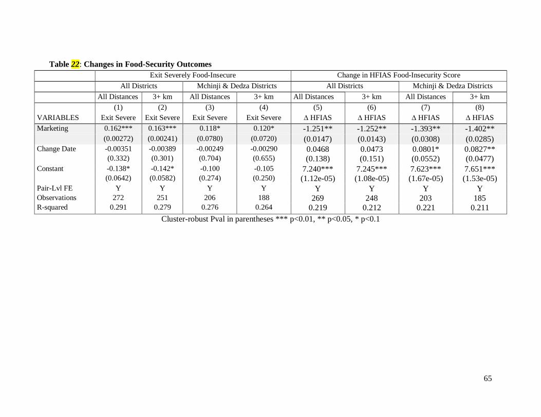
65

Table 22: Changes in Food-Security Outcomes

Exit Severely Food-Insecure Change in HFIAS Food-Insecurity Score All Districts Mchinji & Dedza Districts All Districts Mchinji & Dedza Districts All Distances 3+ km All Distances 3+ km All Distances 3+ km All Distances 3+ km (1) (2) (3) (4) (5) (6) (7) (8) VARIABLES Exit Severe Exit Severe Exit Severe Exit Severe ∆ HFIAS ∆ HFIAS ∆ HFIAS ∆ HFIAS Marketing 0.162*** 0.163*** 0.118* 0.120* -1.251** -1.252** -1.393** -1.402** (0.00272) (0.00241) (0.0780) (0.0720) (0.0147) (0.0143) (0.0308) (0.0285) Change Date -0.00351 -0.00389 -0.00249 -0.00290 0.0468 0.0473 0.0801* 0.0827** (0.332) (0.301) (0.704) (0.655) (0.138) (0.151) (0.0552) (0.0477) Constant -0.138* -0.142* -0.100 -0.105 7.240*** 7.245*** 7.623*** 7.651*** (0.0642) (0.0582) (0.274) (0.250) (1.12e-05) (1.08e-05) (1.67e-05) (1.53e-05) Pair-Lvl FE Y Y Y Y Y Y Y Y Observations 272 251 206 188 269 248 203 185 R-squared 0.291 0.279 0.276 0.264 0.219 0.212 0.221 0.211

Cluster-robust Pval in parentheses *** p<0.01, ** p<0.05, * p<0.1

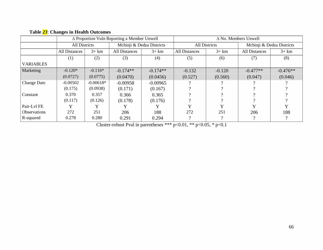
66

Table 23: Changes in Health Outcomes ∆ Proportion Vuln Reporting a Member Unwell ∆ No. Members Unwell All Districts Mchinji & Dedza Districts All Districts Mchinji & Dedza Districts All Distances 3+ km All Distances 3+ km All Distances 3+ km All Distances 3+ km (1) (2) (3) (4) (5) (6) (7) (8) VARIABLES Marketing -0.120* -0.116* -0.174** -0.174** -0.132 -0.120 -0.477** -0.476** (0.0727) (0.0775) (0.0470) (0.0456) (0.527) (0.560) (0.047) (0.046) Change Date -0.00502 -0.00618* -0.00958 -0.00965 ? ? ? ? (0.175) (0.0938) (0.171) (0.167) ? ? ? ? Constant 0.370 0.357 0.366 0.365 ? ? ? ? (0.117) (0.126) (0.178) (0.176) ? ? ? ? Pair-Lvl FE Y Y Y Y Y Y Y Y Observations 272 251 206 188 272 251 206 188 R-squared 0.278 0.280 0.291 0.294 ? ? ? ?

Cluster-robust Pval in parentheses *** p<0.01, ** p<0.05, * p<0.1

67

8. The Indirect Treatment Effect (ITE)

Up until this point, analysis of effects has been limited to the framework of intention to

treat – or, in this case, the indirect effect of the intention to treat (IIT). The ultimate goal,

however, is to determine the causal indirect effects of financial service use expansion itself on

inter-household transfer receipts by non-users. To do this, I regress transfer receipts on the

percentage of households in the local community using formal savings, instrumenting for the

latter with the randomly assigned information intervention.

Since the information on cash gifts was collected only in the endline, I am constrained to

a cross-sectional analysis. That is, in the first stage, I regress local percentage of households with

formal savings in 2010 on the marketing dummy, and in the second stage regress assistance

receipts in 2010 on the instrumented local percentage of households with formal savings.

However, as we have already seen in the panel analysis of the marketing instrument’s effects, it

appears as if the instrument may not have been successful in boosting the local formal savings

use in Lilongwe district. In addition, the marketing-clusters in Lilongwe already had a higher

average level of formal savings use than the non-marketing clusters (though it was shown o be

driven by one or two outliers). I therefore also report results restricting the data to the other two

districts, Dedza and Mchinji.

As the focus here is the indirect effects of local formal savings use, I restrict analysis to

just the highly-vulnerable category. The unit of observation in these regressions is the village-

cluster, and the variables are therefore cluster-level aggregates. The dependent variable is the

cluster mean of the 0-1 variable for receiving a cash gift among just the category-G households.

That is, it is the proportion of the given village cluster’s category-G households that receive a

cash gift. The dependent variable is the cluster mean of the 0-1 variable indicating whether a

household has a formal savings account. That is, it is the proportion of households (among all

households in the cluster) that report having one or more formal savings accounts. This variable

may be endogenous for several possible reasons. For example, integration into the modern

economy may weaken norms for assisting other households (e.g. dilute traditional safety nets and

informal aid networks), and may also increase the probability of having formal savings.

68

Communities whose residents are more integrated into modern life may therefore have higher

formal savings usage rates, and lower gifts among non-users, but not due to an effect of formal

savings on assistance.

The first stage is a simple Linear estimation that regresses the percentage of households

(among everyone) in the village cluster with formal savings on the dummy for marketing. The

unit of observation is the village-cluster, so the dependent variable here is the cluster mean of the

0-1 indicator variable for a household having formal savings in 2010. The regression includes

pair-level fixed effects. I assume it also uses heteroskedasticity-robust standard errors. I am not

absolutely certain, since I am simply using the Stata routine “ivreg 2sls”; I do specify robust

errors, and I think this forces the first stage regression to also use robust standard errors, but I

should check on this. (All I need to do to check is to run the ivreg, and have it report the first

stage along with the second stage, then run the first stage alone using robust standard errors, and

see if the standard errors are the same.)

It should be noted that, since the analysis is restricted to category-G households, I am

forced to drop from the analysis any clusters that do not have any category-G households. This

results in dropping 13 village clusters (11%) from the sample. (I am working on way to redefine

the highly vulnerable category such that each cluster might have at least one, or at least such that

I can drop fewer clusters here). Since the above analysis of the information intervention’s effect

on formal financial services use included these 13 clusters, I repeat the analysis of the

instrument’s effect on local formal savings prevalence leaving out these 13 clusters to give a

more accurate picture of the first stage. As in the previous regressions of the marketing’s effect,

pair-level fixed effects are included, and errors are clustered at the village cluster level. (I also

repeat the analysis on formal credit use, dropping the 13 village clusters without category-G

households, and find the marketing instrument still has no significant effect on cross-sectional

levels or changes in prevalence of formal credit. Results not reported here.)

The results on the marketing’s effect on formal savings prevalence are reported in Table

24. In all samples, the instrument has a highly significant effect on the percentage of households

in the village with formal savings in 2010 (regardless of distance threshold or district). For the

second stage of the cross-sectional IV regressions I run to estimate the indirect effect of formal

savings, this is technically all that matters. However, since I do have a panel on the financial

services variable, a more strict test on the instrument’s strength in inducing the boost in local

69

formal savings prevalence is looking at the two year change induced. Here, we see that the

instrument is not quite significant when including all districts, but is significant at the .05 level

when restricting to the two districts furthest from the capital and the bank headquarters. (As

discussed above, note that this lack of significance in the change in prevalence of formal savings

may be driven by my failure to include the baseline level of formal savings use as a determinant

in the change regression.)

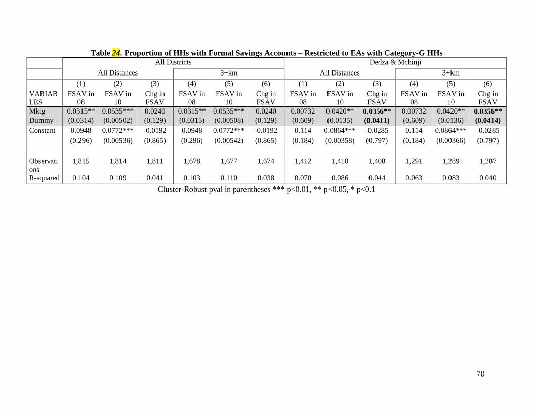
70

Table 24. Proportion of HHs with Formal Savings Accounts – Restricted to EAs with Category-G HHs All Districts Dedza & Mchinji All Distances 3+km All Distances 3+km (1) (2) (3) (4) (5) (6) (1) (2) (3) (4) (5) (6) VARIABLES

FSAV in 08

FSAV in 10

Chg in FSAV

FSAV in 08

FSAV in 10

Chg in FSAV

FSAV in 08

FSAV in 10

Chg in FSAV

FSAV in 08

FSAV in 10

Chg in FSAV

Mktg 0.0315** 0.0535*** 0.0240 0.0315** 0.0535*** 0.0240 0.00732 0.0420** 0.0356** 0.00732 0.0420** 0.0356** Dummy (0.0314) (0.00502) (0.129) (0.0315) (0.00508) (0.129) (0.609) (0.0135) (0.0411) (0.609) (0.0136) (0.0414) Constant 0.0948 0.0772*** -0.0192 0.0948 0.0772*** -0.0192 0.114 0.0864*** -0.0285 0.114 0.0864*** -0.0285 (0.296) (0.00536) (0.865) (0.296) (0.00542) (0.865) (0.184) (0.00358) (0.797) (0.184) (0.00366) (0.797) Observations

1,815 1,814 1,811 1,678 1,677 1,674 1,412 1,410 1,408 1,291 1,289 1,287

R-squared 0.104 0.109 0.041 0.103 0.110 0.038 0.070 0.086 0.044 0.063 0.083 0.040 Cluster-Robust pval in parentheses *** p<0.01, ** p<0.05, * p<0.1

71

The regressions reported in Table 24are not of course the exact regressions I run in the

first stage of my two-stage least squares estimations described above. For the regressions in

Table 24, the unit of observation is the household (with dependent variable a 0-1 indicator for

formal savings), rather than the village-cluster (with dependent variable the mean of the 0-1

values within the cluster). The reason I show the household-based regression is that it should be

more efficient, and provide the most accurate picture of the true effects of the encouragement on

local financial services use. I have not yet generated the tables for the cluster-based regression,

but I assume the levels of significance will drop, since I would use heteroskedastic-robust

standard errors there, rather than explicitly correcting for the heteroskedasticity via weighting

(FGLS) as is automatically done in the household-based regressions reported here in Table 24.

In fact, I would prefer to run the system using as the first stage the regression reported in

Table 24– i.e. using this regression’s coefficient estimates and its standard errors in the second

stage its – since I believe it is the appropriate first stage. But I don’t know how to do this yet – I

may need to write my own code in Matlab or R – since the first stage and second stage are based

on percentages among different samples. (The first stage percentage is based on the entire

sample, whereas the second stage is a percentage of just the vulnerable households). So for now,

the actual first stage in the IV estimations I report below is a regression of the actual cluster-

percentage of households with formal savings in 2010 on the marketing dummy (the cluster

being the observational unit). To the extent that this results in a weaker instrument for endline

local savings prevalence, this would be evident in the second stage, where the estimate for the

instrumented variable would be non-significant. In linear (only linear?) IV regressions with a

just-identified first stage, the standard errors in the second stage can still be trusted even if the

instrument is marginally “weak”.32

The second stage is a simple cross-sectional Linear-IV with the endline data, where I

regress the percentage of category-G households that receive a cash gift on the predicted

percentage of households in the cluster with formal savings. I include pair-level fixed effects.

There is of course no reason to cluster at the EA-level, since here the EA is the unit of

observation. I also use Huber-White sandwich errors to account for heteroskedasticity caused by

use of variables that are percentages with variation in the number of observations used to

32 Angrist and Pischke, Mostly Harmless Econometrics, as well as their follow-up note on this, published online.

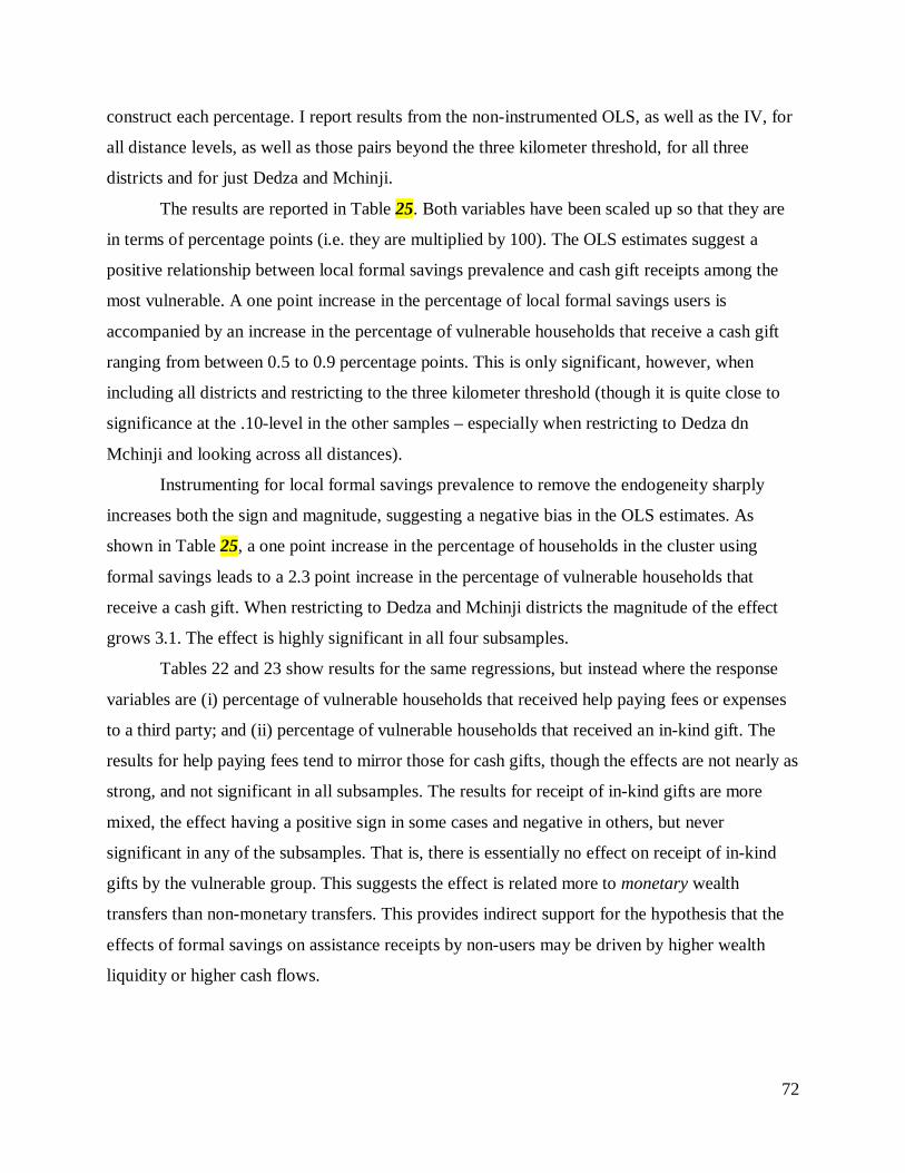
72

construct each percentage. I report results from the non-instrumented OLS, as well as the IV, for

all distance levels, as well as those pairs beyond the three kilometer threshold, for all three

districts and for just Dedza and Mchinji.

The results are reported in Table 25. Both variables have been scaled up so that they are

in terms of percentage points (i.e. they are multiplied by 100). The OLS estimates suggest a

positive relationship between local formal savings prevalence and cash gift receipts among the

most vulnerable. A one point increase in the percentage of local formal savings users is

accompanied by an increase in the percentage of vulnerable households that receive a cash gift

ranging from between 0.5 to 0.9 percentage points. This is only significant, however, when

including all districts and restricting to the three kilometer threshold (though it is quite close to

significance at the .10-level in the other samples – especially when restricting to Dedza dn

Mchinji and looking across all distances).

Instrumenting for local formal savings prevalence to remove the endogeneity sharply

increases both the sign and magnitude, suggesting a negative bias in the OLS estimates. As

shown in Table 25, a one point increase in the percentage of households in the cluster using

formal savings leads to a 2.3 point increase in the percentage of vulnerable households that

receive a cash gift. When restricting to Dedza and Mchinji districts the magnitude of the effect

grows 3.1. The effect is highly significant in all four subsamples.

Tables 22 and 23 show results for the same regressions, but instead where the response

variables are (i) percentage of vulnerable households that received help paying fees or expenses

to a third party; and (ii) percentage of vulnerable households that received an in-kind gift. The

results for help paying fees tend to mirror those for cash gifts, though the effects are not nearly as

strong, and not significant in all subsamples. The results for receipt of in-kind gifts are more

mixed, the effect having a positive sign in some cases and negative in others, but never

significant in any of the subsamples. That is, there is essentially no effect on receipt of in-kind

gifts by the vulnerable group. This suggests the effect is related more to monetary wealth

transfers than non-monetary transfers. This provides indirect support for the hypothesis that the

effects of formal savings on assistance receipts by non-users may be driven by higher wealth

liquidity or higher cash flows.

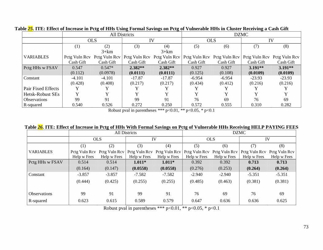
73

Table 25. ITE: Effect of Increase in Pctg of HHs Using Formal Savings on Pctg of Vulnerable HHs in Cluster Receiving a Cash Gift

All Districts DZMC OLS IV OLS IV (1) (2)

3+km (3) (4)

3+km (5) (6) (7) (8)

VARIABLES Pctg Vuln Rcv Cash Gift

Pctg Vuln Rcv Cash Gift

Pctg Vuln Rcv Cash Gift

Pctg Vuln Rcv Cash Gift

Pctg Vuln Rcv Cash Gift

Pctg Vuln Rcv Cash Gift

Pctg Vuln Rcv Cash Gift

Pctg Vuln Rcv Cash Gift

Pctg HHs w FSAV 0.547 0.547* 2.382** 2.382** 0.927 0.927 3.191** 3.191** (0.112) (0.0978) (0.0111) (0.0111) (0.125) (0.108) (0.0109) (0.0109) Constant -4.101 -4.101 -17.87 -17.87 -6.954 -6.954 -23.93 -23.93 (0.428) (0.408) (0.217) (0.217) (0.434) (0.412) (0.216) (0.216) Pair Fixed Effects Y Y Y Y Y Y Y Y Hetsk-Robust SEs Y Y Y Y Y Y Y Y Observations 99 91 99 91 76 69 76 69 R-squared 0.540 0.526 0.272 0.250 0.572 0.555 0.310 0.282

Robust pval in parentheses *** p<0.01, ** p<0.05, * p<0.1

Table 26. ITE: Effect of Increase in Pctg of HHs With Formal Savings on Pctg of Vulnerable HHs Receiving HELP PAYING FEES All Districts DZMC OLS IV OLS IV (1) (2) (3) (4) (5) (6) (7) (8) VARIABLES Pctg Vuln Rcv

Help w Fees Pctg Vuln Rcv Help w Fees

Pctg Vuln Rcv Help w Fees

Pctg Vuln Rcv Help w Fees

Pctg Vuln Rcv Help w Fees

Pctg Vuln Rcv Help w Fees

Pctg Vuln Rcv Help w Fees

Pctg Vuln Rcv Help w Fees

Pctg HHs w FSAV 0.514 0.514 1.011* 1.011* 0.392 0.392 0.713 0.713 (0.164) (0.147) (0.0558) (0.0558) (0.276) (0.253) (0.264) (0.264) Constant -3.857 -3.857 -7.582 -7.582 -2.940 -2.940 -5.351 -5.351 (0.444) (0.425) (0.255) (0.255) (0.485) (0.463) (0.381) (0.381) Observations 99 91 99 91 76 69 76 69 R-squared 0.623 0.615 0.589 0.579 0.647 0.636 0.636 0.625

Robust pval in parentheses *** p<0.01, ** p<0.05, * p<0.1

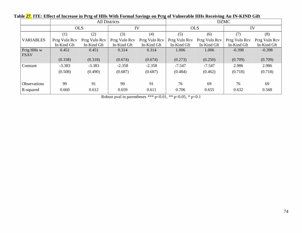
74

Table 27. ITE: Effect of Increase in Pctg of HHs With Formal Savings on Pctg of Vulnerable HHs Receiving An IN-KIND Gift All Districts DZMC OLS IV OLS IV (1) (2) (3) (4) (5) (6) (7) (8) VARIABLES Pctg Vuln Rcv

In-Kind Gft Pctg Vuln Rcv

In-Kind Gft Pctg Vuln Rcv

In-Kind Gft Pctg Vuln Rcv

In-Kind Gft Pctg Vuln Rcv

In-Kind Gft Pctg Vuln Rcv

In-Kind Gft Pctg Vuln Rcv

In-Kind Gft Pctg Vuln Rcv

In-Kind Gft Pctg HHs w FSAV

0.451 0.451 0.314 0.314 1.006 1.006 -0.398 -0.398

(0.338) (0.318) (0.674) (0.674) (0.273) (0.250) (0.709) (0.709) Constant -3.383 -3.383 -2.358 -2.358 -7.547 -7.547 2.986 2.986 (0.508) (0.490) (0.687) (0.687) (0.484) (0.462) (0.718) (0.718) Observations 99 91 99 91 76 69 76 69 R-squared 0.660 0.612 0.659 0.611 0.706 0.655 0.632 0.568

Robust pval in parentheses *** p<0.01, ** p<0.05, * p<0.1

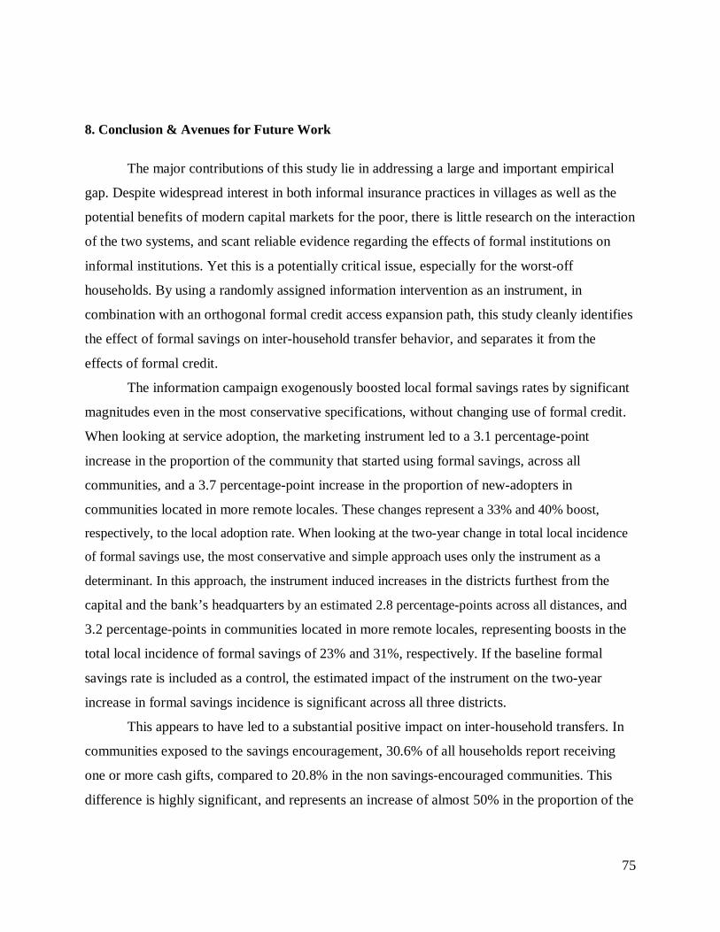
75

8. Conclusion & Avenues for Future Work

The major contributions of this study lie in addressing a large and important empirical

gap. Despite widespread interest in both informal insurance practices in villages as well as the

potential benefits of modern capital markets for the poor, there is little research on the interaction

of the two systems, and scant reliable evidence regarding the effects of formal institutions on

informal institutions. Yet this is a potentially critical issue, especially for the worst-off

households. By using a randomly assigned information intervention as an instrument, in

combination with an orthogonal formal credit access expansion path, this study cleanly identifies

the effect of formal savings on inter-household transfer behavior, and separates it from the

effects of formal credit.

The information campaign exogenously boosted local formal savings rates by significant

magnitudes even in the most conservative specifications, without changing use of formal credit.

When looking at service adoption, the marketing instrument led to a 3.1 percentage-point

increase in the proportion of the community that started using formal savings, across all

communities, and a 3.7 percentage-point increase in the proportion of new-adopters in

communities located in more remote locales. These changes represent a 33% and 40% boost,

respectively, to the local adoption rate. When looking at the two-year change in total local incidence

of formal savings use, the most conservative and simple approach uses only the instrument as a

determinant. In this approach, the instrument induced increases in the districts furthest from the

capital and the bank’s headquarters by an estimated 2.8 percentage-points across all distances, and

3.2 percentage-points in communities located in more remote locales, representing boosts in the

total local incidence of formal savings of 23% and 31%, respectively. If the baseline formal

savings rate is included as a control, the estimated impact of the instrument on the two-year

increase in formal savings incidence is significant across all three districts.

This appears to have led to a substantial positive impact on inter-household transfers. In

communities exposed to the savings encouragement, 30.6% of all households report receiving

one or more cash gifts, compared to 20.8% in the non savings-encouraged communities. This

difference is highly significant, and represents an increase of almost 50% in the proportion of the

76

community reporting cash-gift receipts in moving from the non-encouraged to the savings-

encouraged villages.

The positive impacts of the savings-encouragement on receipts of inter-household

assistance systematically increase as vulnerability heightens. Among the least vulnerable 14% of

the sample (households in categories A and B), cash gift receipts are no higher in the

information-treated communities. Yet the difference becomes significant within households in

vulnerability category C, with a difference of 10.4 percentage-points, growing to 10.6

percentage-point among category D, 10.9 among category E, 11.5 among category F, and 17.8

among Category G. The striking impact on receipt of inter-household transfers by the most

vulnerable group underscores the fact that the impacts of financial deepening may be especially

large on the worst-off households, a group of particular policy-importance for many anti-poverty

and development initiatives.

To more accurately quantify the nature of this impact on the most vulnerable, fixed

effects were added and errors were clustered at the community-level, in a linear regression of

receipt of a cash-gift on the information-treatment dummy. This indirect intention to treat (IIT)

analysis showed IIT estimates of the impact on the highly vulnerable’s probability of receiving a

gift ranging from 15.3 to 15.9 percentage-points, which were highly significant. Results were

almost identical in a Probit specification. An instrumental-variables regression then enabled an

estimate of the full indirect treatment effect (ITE) of increases in the proportion of formal savers

on the percentage of highly vulnerable that received one or more cash gifts. This analysis showed

ITE estimates indicating that a one percentage-point increase in the local proportion of formal-

savers led to a 2.4 to 3.2 percentage-point increase in the proportion of highly vulnerable

households that received one or more cash-gifts.

As minimum balances and fixed costs associated with opening a formal account create a

barrier preventing use by the poorest, the highly vulnerable group is de facto ineligible to take up

formal savings. These strong impacts on receipts of inter-household transfers by the most

vulnerable are therefore clear evidence of a spillover effect of formal savings adoption on non

formal-savers. This adds to a small but growing number of studies that highlight the importance

of accounting for and measuring indirect impacts of policy interventions and aid programs.

These effects can be of critical importance, particularly in village-settings, where households are

often intimately connected with each other. The impact evaluation literature tends to remain

77

focused on assessments of program effects on direct beneficiaries of the program. While perhaps

natural, it is clear that in some cases very large effects may lie outside this narrow focus, and

significant portions of a project’s impact may be missed entirely when failing to account for

indirect effects on the putatively “non-treated”.

The findings of this study carry significant methodological import in particular for impact

assessments in microfinance, an increasingly common research activity in development. The

results show that the provision of financial services has important indirect effects on local-area

households. This means that within-locality comparisons, even when suitable instruments are

available or randomized access is feasible, can be an invalid and unreliable method for

measuring the effects of of service-use. Thus, approaches based on local-average treatment

effects (LATE) must be implemented and interpreted with extreme caution, and should not be

used to infer absolute direct impacts unless it can be verified that the SUTVA assumption

actually holds. Perhaps most importantly, this suggests that measuring the full impacts of

microfinance projects and interventions to expand access to formal capital markets, requires a

broader focus on the entire community of which service-users form a part.

This study’s empirical findings on the response of receipts of monetary assistance (gifts

and loans) to formal savings expansion are important in their own right, not least because of

previous suggestions the effect may be in the opposite direction. However, as Townsend (1994)

rightly points out, by narrowing the focus to only a few institutions (e.g. gifts and loans), it is of

course always possible to miss parallel changes in other consumption-smoothing options. While

all observable indicators suggest that the increased monetary assistance did not substitute for

assistance that would have been received in other forms, it is nevertheless possible the data fail

to capture consequent effects on other smoothing mechanisms available to the ultra-poor.

The data, however, permit the analysis to proceed several steps further, by analyzing the

consequent impact on welfare outcomes. The absence of typical consumption data and reliable

income information precludes standard efficiency-tests of the sort employed by Townsend

(1995). If the data contained this information, it would be possible to check whether

consumption of highly vulnerable households in the savings-promotion villages tracks

movements in village-level consumption more closely than that of highly vulnerable households

in the non-marketing villages. Yet a general equilibrium approach which overcomes the pitfalls

of looking at the impacts on individual institutions one at a time is still possible. By examining

78

the welfare outcomes of the households affected, it is possible to implicitly infer whether any

substitution or displacement effects neutralize the positive benefits to recipient households. It

also focuses the analysis squarely on outcomes of crucial policy relevance: the well-being of the

poor.

This study’s results show that living in communities that received the saving

encouragement caused two-year improvements in at least three key welfare indicators among the

worst-off. Highly vulnerable households are 11.8 to 16.3 percent more likely to exit the worst

food-security category in the HFIAP scale (severely insecure) to enter one of the three other less

severe categories. They also experience a 1.3 to 1.4 reduction in the continuous food-insecurity

score, HFIAS, representing a 10-12% improvement in food-security over baseline values. In

addition, highly vulnerable households living in savings-encouraged communities were 12 to

17.4 percent less likely to report any members of the household as recently unwell.

One of the most noteworthy findings of this study is the impressive magnitude of the

effects on transfer receipts – particularly among the worst-off households – and the substantial

impacts this has on welfare outcomes. While certainly promising, the lesson here should be one

of caution. Recall that the model predicts an ambiguous result, making it possible for the

introduction of formal savings to have a stimulating effect on inter-household wealth flows. It is

not clear, however, that introducing formal savings will always have a positive effect. The results

of this study quite clearly demonstrate that expanding formal savings access can have very large

effects on inter-household transfer behaviors, and that changes in transfer receipts can have

substantial impacts on the welfare of the poorest of the poor. While the fact that the experience

of rural Malawi was in the positive direction is perhaps a promising sign, the model suggests this

result depends on the shape of preferences. It is possible that preferences or cultural norms in

Central Malawi differ in some relevant way such that its experience would differ from that of

other areas.33

33 As an example, this region is predominantly Chewa, an ethnic group that is historically matrilineal and matrilocal. Research elsewhere has shown the importance of matrilineal institutions, such as land-inheritance and post-marital location practices, on behavior (e.g. Gneezy, Leonard, and List 2009; Flory, Leonard, and List 2011). In particular, List et. al. (??) find evidence that individuals in matrilineal societies may contribute more to public goods. If matrilineal customs are somehow linked to the strength and prevalence of “social preferences”, it may affect the ways in which the findings of this study apply to other settings. Further research on the relationship between land-

79

Another important caveat is with respect to time-frame. Two years is a relatively short

period for the materialization of impacts, and there may be countervailing effects which operate

over a longer time-frame. For example, behavioral habits and social norms may change but on a

slower scale. It may be, for example, that five to ten years after the expansion of formal savings,

the effect on inter-household wealth transfers is reversed if the hypothetical drivers elaborated by

FR00 and LTW00 materialize. In this case, if financial markets do not develop quickly enough,

so that all households have access, the outcome could be more mixed, with potentially negative

outcomes for highly vulnerable households whose previous safety nets have been displaced,

without adequate substitutes. In this case, policy-makers and practitioners will want to be more

careful to see that promoting the expansion of formal savings options is accompanied by

substitutes for safety nets which may disappear for the most vulnerable. Identifying whether the

effects identified in this study change over time, and perhaps reverse, thus represents a critical

avenue for future research.

Finally, at a methodological level, though not the point of the study, this represents one of

the first explicit empirical analyses of the indirect effects of an intention to treat that I am aware

of. The possibility of the existence of indirect effects from the intention to treat is emphasized in

discussions of issues such as violation of SUTVA (stable unit treatment value assumption), and

the complications this poses for the validity of instrumental-variables approaches relying on

intention-to-treat as an instrument, e.g. discussions of LATE estimates of impacts in the program

evaluation literature. However, little attention appears to be paid to understanding the indirect

effects of an intention to treat as an object of analysis in its own right. Of course the ultimate

point of this study’s analysis of indirect effects is to understand the actual indirect treatment

effect (i.e. the indirect effect on non-users of formal savings use), and the IIT-analysis is an

intermediate stage and important signal of the ITE’s presence. However, it bares mentioning that

this is one of the first studies I am aware of to use an empirical approach which includes

inheritance and post-marital location practices on the one hand and gift-giving behavior to provide consumption insurance is may be necessary.

80

examining the impacts of the intention to treat on non-beneficiaries.34

Use of the simple IIT

estimator may be of benefit to future impact evaluations.

7.2. Towards a More Comprehensive Theory of Institutional Change

While not its central purpose, this study also makes some contributions on a theoretical

dimension. As early as 1995, Timothy Besley identified the absence of a theory of institutional

formation and adaptation as the key component missing from analyses of non-market institutions

for addressing risk, highlighting the need for better models of “how institutions are born, grow,

change, and develop.” This study contributes in important ways to the project of developing an

integrated theory on institutional change, furnishing evidence on how indigenous practices

respond to the expansion of modern economic institutions. That the experience of villages in

Central Malawi contradicts initial suggestive indications mentioned in passing by Townsend

(1994) and Besley (1995), as well as more rigorously developed theoretical predictions of FR,

underscores the challenge of developing a robust unified theory in this area. Besley (95)

emphasizes that the iterative process demonstrated in Townsend (94), through which data and

theory confront each other in the development of more accurate models, would become

increasingly important in research on informal institutions. To that end, models of the impacts of

formal financial services on informal insurance institutions might benefit from qualifications or

adjustments to account for the deviations from the model documented here, in order to provide a

more complete representation of changes we can expect in the future as modern financial

institutions encounter pre-modern practices (which evolved to fulfill similar functions), with

ever-growing frequency.

The empirical results appear to run counter to predicted outcomes of models premised on

assumptions of bidirectional transfers motivated by promises of future reciprocation, which

dominate the literature on informal insurance in villages. That the experience of rural households

34 Though they introduce the ITE as a novel estimand for impact evaluations, Angelucci et. al. (2009) did not include an analysis of indirect intention to treat, as there was almost 100% compliance among eligibles in their sample. As the program they were discussing was welfare payments from the government, almost all those who were eligible chose to be treated. In the present context of wealth-constrained access to formal savings, however, the non-eligibles easiest to identify are the poorest households (group G). Those defined as “eligible” (potentially anyone not in group G) had a compliance rate far less than 100%, creating the need to distinguish between an indirect treatment effect (ITE, as in Angelucci et. al.) and an indirect intention to treat effect (IIT).

81

in Central Malawi is at odds with key implications of the sparse theoretical work on this question

suggests the need for theoretical innovation and models which better accommodate the expanded

set of empirical data the present study brings to this thin literature. This suggests a broadening of

the accepted theoretical underpinnings of inter-household informal insurance arrangements may

be in order. The empirical findings of the present study also underscore the need for theory

which captures the indirect effects of changes in intertemporal wealth transfer and risk-sharing

technologies on those who do not or cannot use the new tools.

As a small step in that direction, a simple theoretical framework contrasted an

investment, or insurance-purchasing decision, against a two-period model of consumption and

charitable giving. The model suggests that transfers predicated on expected future reciprocation

unambiguously decline when formal savings is adopted, while the latter allows for an ambiguous

result. The model also suggests that, when transfers are motivated by issues of expected

reciprocation, self-insurance, and saving, adopting formal savings should cause a household to

decrease its loans to those least likely to repay (or likely to repay less than the amount given)

first. That is, it will place less of its savings in the inferior investments. These inferior savings

options are most likely to be disproportionately represented by the worst-off households. So loan

receipts by the worst off should decrease The fact that inter-household transfers increased rather

than decreased, particularly among the worst-off, suggests that factors associated with

unidirectional wealth-flows can be an important driver of inter-household transfer behavior. The

extent to which self-insurance motives versus charitable-giving motives drive transfer decisions

are likely to have important practical implications relevant to development and poverty policy.

Identifying the factors that cause transfers to be perceived as insurance, or instead as a non-

reciprocated gift, thus represents an important path for future research.

Another important question which remains to be answered is whether unidirectional gifts

are driven by intrinsic or extrinsic factors, and – if the latter – whether from the imposition of

pressure to share or perhaps instead the desire to earn admiration and respect. The answers to

these questions will help determine the most plausible impacts on inter-household transfer

practices and welfare outcomes of the poor in response to continued financial deepening and

other external shocks, stimuli, or adjustments that occur as part of the transition process towards

modern economies.

82

References Adelman, Sarah, and Geetha Nagarajan (2009). “Who Des Formal Finance Reach in Rural Malawi?” IRIS Center, University of Maryland, December 2009. Arimond, Mary, and Marie T. Ruel (2004). “Dietary diversity is associated with child nutritional status: evidence from 11 demographic and health surveys”. Journal of Nutrition 2004; 134(10): 2579–85. Coates, Swindale, and Coates J, Swindale A, Bilinsky P. Household Food Insecurity Access Scale (HFIAS) for Measurement of Household Food Access: Indicator Guide (v.3).Washington, DC: Food and Nutrition Technical Assistance Project, Academy for Educational Development; August 2007. Fafchamps, M., & Gabre-Madhin, E. (2001). “Agricultural markers in Benin and Malawi: The operation and performance of traders.” Policy Research Working Paper 2734. Washington, DC: World Bank Development Research Group, Rural Development. McGuinness, Elizabeth (2008). “Malawi’s Financial Landscape: Where Does Opportunity International Bank of Malawi Fit in?”, Microfinance Opportunites, July 2008. Available online at: http://fsassessment.umd.edu/publications/pdfs/OIBM-Financial-Landscape.pdf Meagher, Patrick (2010). “Constant Gardening: A Study of Malawi’s Enabling Enviornment for Microfinance. “ IRIS Center, University of Maryalnd, July 2010. Available online at http://fsassessment.umd.edu/publications/pdfs/Malawi-Environment-Studies.pdf

Flory, Jeffrey and Geetha Nagarajan. “The Poor and their Management of Shocks”, IRIS Center

Report for “Assessing the Impact of Innovation Grants in Financial Services”, University of

Maryland. December, 2009.

Available online at: http://www.fsassessment.umd.edu/publications/pdfs/Malawi-Shock-

Management.pdf

Alderman, H., J. Hoddinott, and B. Kinsey. 2006. “Long-term consequences of early childhood

malnutrition.” Oxford Economic Papers 58: 450–474.

83

Angelucci, Manuela and Giacomo De Giorgi, 2009. “Indirect Effects of an Aid Program: How do Cash Transfers Affect Non-Eligibles Consumption?" American Economic Review, 99, 486-509. Antle, John M., "Econometric Estimation of Producers' Risk Attitudes," American Journal of Agricultural Economics, August 1987, 69:3, 509-22. Arnott, Richard, and Joseph E. Stiglitz,1991. "Moral Hazard and Nonmarket Institutions: Dysfunctional Crowding Out or Peer Monitoring," American Economic Review, 1990, 81:1,179-90.

Banerjee, A. (2005). "The two poverties". In: Dercon, S., (Ed.), Insurance Against Poverty. Oxford University Press, Oxford.

Beegle, Kathleen, and Rajeev H. Dehejia, Roberta Gatti, “Child labor and agricultural shocks,” Journal of Development Economics, Volume 81, Issue 1, October 2006, Pages 80-96,

Besley, T. (1995a). Nonmarket institutions for credit and risk sharing in low-income countries. Journal of Economic Perspectives, 9, 115–127.

Besley, Timothy. 1995b Chapter 36 Savings, credit and insurance, In: Jere Behrman and T.N.

Srinivasan, Editor(s), Handbook of Development Economics, Elsevier, Volume 3, Part 1, Pages

2123-2207,

Besley & Coate (1995) “Group Lending, Repayment Incentive, and Socail Capital” Journal of

Development Economics

Binswanger, Hans, and Mark Rosenzweig, "Wealth, Weather Risk and the Composition and Profitability of Agricultural Investments," Economic Journal, January 1993, 103, 56-78.

Bliss, Christopher, and Nicholas Stern, Palanpur: The Economy of an Indian Village. Oxford: Oxford University Press, 1982.

Coate, S., Ravallion, M., 1993. “Reciprocity without commitment: characterization and performance of informal insurance arrangements.” Journal of Development Economics 40, 1– 24.

84

Cox, Donald, and Emmanuel Jimenez , 1995 "Private Transfers and the Effectiveness of Public

Income Redistribution in the Philippines." In Dominique van de Walle and Kimberly Nead, eds.,

Public Spending and the Poor: Theory and Evidence. Baltimore: Johns Hopkins University Press.

Cox, Donald, and Emmanuel Jimenez , 1998. "Risk-Sharing and Private Transfers: What about

Urban Households?"Economic Development and Cultural Change 46(3):621-39.

Deaton, A. 1992. Understanding consumption. Oxford: Clarendon Press.

Deaton, Angus. 1997. The Analysis of Household Surveys: A Microeconometric Approach to Development Policy. Baltimore: Johns Hopkins University Press.

Dercon, S. (2005). Insurance Against Poverty. Oxford University Press, Oxford.

Dercon, S. (2005). "Risk, insurance, and poverty: a review". In: Dercon, S., (Ed.), Insurance Against Poverty. Oxford University Press, Oxford.

Dercon, S., Hoddinott, J. (2005). "Health, shocks, and poverty persistence". In: Dercon, S., (Ed.), Insurance Against Poverty. Oxford University Press, Oxford.

Dercon, Stefan, John Hoddinott, Pramila Krishnan and Tassew Woldehannna 2008. “Collective

Action and Vulnerability: Burial Societies in Rural Ethiopia.” Collective Action and Property

Rights working paper no 83. Washington D.C.: International Food Policy Research Institute.

Fafchamps, M.. 1992. Solidarity networks in rural Africa: rational peasants with a moral

economy. Economic Development and Cultural Change 41:1, 147-174.

Fafchamps, Marcel (1999). “Risk-Sharing and Quasi-Credit”. Journal of Interational Trade &

Economic Development. 8:3 257-278.

85

Fafchamps, M. and S. Lund (2003) “Risk Sharing Networks in Rural Philippines," Journal of Development Economics 71, 261-87.

Fafchamps, Marcel, Christopher Udry, and Katherine Czukas, (1998) .” Drought and Saving in West Africa: Are Livestock a Bu¤er Stock?” Journal of Development Economics, Vol. 55, pp. 273-305.

Foster, A. (1995). "Prices, credit markets and child growth in low-income rural areas". Economic Journal 105, 551-570.

Foster, A., Rosenzweig, M., 2000. “Financial intermediation, transfers, and commitment: do banks crowd out private insurance arrangements in low-income rural areas?” In: Mason, A., Tapinos, G. (Eds.), Sharing the Wealth: Demographic Changes and Economic Transfers Between Generations. Oxford Univ. Press, Oxford, pp. 207–228.

Giles, J. 2006. "Is life more risky in the open? Household risk-coping and the opening of China's labor markets." Journal of Development Economics 81 (1): 25-60.

Giles, John and Kyeongwon Yoo (2007) “Precautionary Behavior, Migrant Networks and Household Consumption Decisions: An Empirical Analysis Using Household Panel Data from Rural China” The Review of Economics and Statistics, 89(3): 534-551.

Heckman, J., R. Lalonde, and J. Smith (1999): “The Economics and Econometrics of Active Labor Market Programs,” in Handbook of Labor Economics, Vol. 3, ed. byO. Ashenfelter and D. Card. Amsterdam: North-Holland, 1865–2086.

Hoddinott, J. and Kinsey, B. (2001), Child Growth in the Time of Drought. Oxford Bulletin of

Economics and Statistics, 63: 409–436.

Jalan, Jyotsna, and Martin Ravallion. (1999). "Are the Poor Less Well Insured? Evidence on

Vulnerability to Income Risk in Rural China." Journal of Development Economics 58, 61-82.

Jalan, J., Ravallion, M. (2004). "Household income dynamics in rural China". In: Dercon, S., (Ed.), Insurance Against Poverty. Oxford University Press, Oxford.

86

Jensen, Robert T., 2004 “Do private transfers ‘displace’ the benefits of public transfers?

Evidence from South Africa” Journal of Public Economics, 2004, 88, 1-2, 89-112

Jacoby, H. G., Skoufias, E. (1997). "Risk, Financial Markets, and Human Capital in a Developing Country". Review of Economic Studies 64, 311-335.

Karlan, Dean and Jonathan Morduch (2009). “Access to finance,” Chapter 2 in M. Rosenzweig and D. Rodrik (eds.) Handbook of Development Economics, Volume 5.

Kletzer and Wright (1992) “Sovereign Debt Renegotiation in a consumption-smoothing model”

Ligon, Ethan, Jonathan P. Thomas and Tim Worrall. 2000. “Mutual Insurance, Individual Savings, and Limited Commitment.” Review of Economic Dynamics. 3, pp. 216-246.

Miguel, E., and M. Kremer, (2004), “Worms: Identifying Impacts on Education and Health in the Presence of Treatment Externalities,” Econometrica, 72(1), 159-217.

Morduch, Jonathan (1990), "Risk, Production, and Saving: Theory and Evidence from Indian Households," Mimeo, Harvard University, 1990.

Morduch, Jonathan. 1995. "Income Smoothing and Consumption Smoothing," J. Econ. Perspect.

9:3, pp. 103-14.

Morduch, J. 1999a. "Between the state and the market: can informal insurance patch the safety net?". World Bank Research Observer 14:2 187-207.

Morduch, J. 1999b. “The Microfinance Promise,” Journal of Economic Literature, 37, pp 1569-

1614.

Morduch, J. (2006). "Micro-insurance: the next revolution? What have we learned about poverty?". In: Banerjee, A., Benabou, R., Mookherjee, D., (Eds.), Understanding Poverty. Oxford University Press, New York.

87

Paulson, Anna, “Insurance Motives for Migration: Evidence from Thailand,” Kellogg Graduate School of Management, Northwestern University, mimeo, 2000.

Paxson, Christina,(1992) "Using Weather Variability to Estimate the Response of Savings to Transitory Income in Thailand," American Economic Review, 82:1, 15-33.

Platteau, Jean-Philippe, and Anita Abraham.1 987. "An Inquiry into Quasi-Credit Contracts: The

Role of Reciprocal Credit and Interlinked Deals in Small-Scale Fishing Communities." Journal

of Development Studies 23(4):461-90.

Rose, E. (1999). "Consumption smoothing and excess female mortality in rural India". Review of Economics and Statistics 81, 41-49.

Rosenzweig, Mark R. and Oded Stark. 1989. “Consumption Smoothing, Migration and Marriage: Evidence from Rural India.” Journal of Political Economy. 97, 4 pp. 905-927.

Rosenzweig, Mark and Kenneth Wolpin (1993) "Credit Market Constraints, Consumption Smoothing, and the Accumulation of Durable Production Assets in Low: income Countries: Investment in Bullocks in India", Journal of Political Economy, 101 (21): 223-244.

Stiglitz, Joseph E., 1990. "Peer Monitoring and Credit Markets," World Bank Economic Review, 4:3, 351-66.

Townsend, R. (1994). "Risk and Insurance in Village India". Econometrica 62, 539-591.

Townsend, Robert. 1995a. "Consumption Insurance: An Evaluation of Risk-Bearing Systems in

Low-Income Countries."Journal of Economic Perspectives 9: 83-102.

Townsend, Robert. 1995b." Financial Systems in Northern Thai Villages."Quarterly Journal of

Economics 110(November): 1011-46.

88

Townsend, Robert M., and Kenichi Ueda. 2006. “Financial Deepening, Inequality and Growth: A Model-Based Quantitative Evaluation.” Review of Economic Studies, 73 (1): 251–93. Udry, C. (1994). "Risk and Insurance in a Rural Credit Market: An Empirical Investigation in Northern Nigeria". Review of Economic Studies 61, 495-526.

Wade, Robert, 1988. Village Republics: Economic Conditions for Collective Action in South

India. Cambridge: Cambridge University Press,

Walker, Thomas S., and James G. Ryan, Village and Household Economies in India's Semi-Arid Tropics. Baltimore, Md.: Johns Hopkins University Press, 1990.

Zeller, M. (1999). The role of micro-finance for income and consumption smoothing. Paper

Presented at the IADB Conference on Social Protection and Poverty. Washington DC, 5

February.