Embed Size (px)
Citation preview

1
Micro-level adaptation, macro-level selection, and the dynamics of
market partitioning
César García-Díaz
Department of Industrial Engineering, Universidad de los Andes (Colombia)
Arjen van Witteloostuijn
Tilburg School of Economics and Management, Tilburg University (the Netherlands)
Antwerp Centre of Evolutionary Demography (ACED), University of Antwerp (Belgium)
Gábor Péli
Utrecht School of Economics, Utrecht University (the Netherlands)
December 11, 2014
Abstract
This paper provides a micro-foundation for dual market structure formation through
partitioning processes in marketplaces by developing a computational model of
interacting economic agents. We propose an agent-based modeling approach, where
firms are adaptive and profit-seeking agents entering into and exiting from the market
according to their (lack of) profitability. Our firms are characterized by large and
small sunk costs, respectively. They locate their offerings along a unimodal demand
distribution over a one-dimensional product variety, with the distribution peak
constituting the center and the tails standing for the peripheries. We compare our
findings to the predictions of earlier dual-market explanations that focus on the macro
(industry/population) level, pointing to commonalities, but also revealing a number of
aspects for which our model extends knowledge on the pre-conditions and
mechanisms of dual market formation. One novel result is the emergence of an
endogenous minimum scale of production for low sunk cost firms that contributes to
the stability of the dual structure. The withdrawal of large firms from the market

2
periphery (enabling the small enterprises to scavenge on residual demand) is a well-
known mechanism of dual structure formation. We found bi-directional center-
periphery moves under a broad range of parameterizations: large firms may first
advance toward the most abundant demand spot, the market center, and release
peripheral positions as predicted by extant dual market explanations. Afterwards,
large firms may then move back toward the market fringes to reduce competitive
niche overlap in the center, triggering nonlinear resource occupation behavior.
Keywords: dual market structure, sunk cost, agent-based simulation, organizational
niche, micro-level adaptation, micro-level economic behavior
1. Introduction
Many industries feature dual market structures, with a few large companies dominated
the market’s center and many smaller enterprises surviving in the market’s periphery.
Such dual market structures are associated with high concentration and high density.
In industrial organization and organization theory, the question as to how dual market
structures of two dominant firm types evolve has been studied since a long time [1, 2,
3]. However, to date, alternative explanations circulate in the literature that have not
yet been integrated [4], implying that the evolution of dual market structures still not
fully understood [5]. In this paper, we develop an agent-based simulation model to
explore different dual market structure explanations, revealing how they can or cannot
be integrated, and what additional mechanisms may well play a role.
Hitherto, little has been done in order to fully incorporate dynamic firm behavior in
the selection-adaptation interplay in the context of population-level market
positioning processes. A comprehensive understanding of the emergence and
evolution of specific market structures should include insights from different
perspectives. Key is that a microeconomic approach can provide the building blocks
for a theory that offers a micro-foundation for macro-level market structuration
processes [5, 6]. We argue that the development of such a micro-foundation in the
form of explicitly modeling firm-level rules of behavior and interaction may indeed
be an important contribution by integrating different arguments in the context of the

3
study of market structures. We seek to integrate firm-level decision-making rules [7]
in the context of horizontal product differentiation [8] into an industry-level approach
through an agent-based computational model.
Our agent-based simulation model connects micro- and macro-level aspects of dual
market formation. It runs in a one-dimensional commodity space [9] with a unimodal
(peaked) demand distribution. Firms address audience tastes concerning product
variants represented as ordered positions along the axis. We consider entry,
competition, and (potential) coexistence of two types of agents: L-firms with large
sunk costs and S-firms with low sunk costs. These agents can also differ in size and in
their breadth of offerings for their respective audience (niche width).
This choice of settings relates our model to two extant dual market theories, one from
Economics and one from Sociology. The unimodal demand distribution, with the
demand peak representing a market center surrounded by peripheries, connects our
approach to the (original version) of resource partitioning theory of sociological
Organizational Ecology (OE) proposed by [2]. This model version is based on
demand release at the market fringes inviting small firm entry to highly concentrated
markets.1 Letting firms with low/high sunk cost operate in this demand landscape
establishes a link to the economic dual structure explanation of [1] in Industrial
Organization (IO). By choosing this configuration, we also aim at getting new insights
on the commonalities between these theories’ underlying disciplinary domains – IO
and OE, respectively – known to exist but unexplored for about two decades [6].
From an IO perspective, [1] explains how game-theoretic equilibria might lead firms
to incur short-run (so-called endogenous) sunk costs. This is the result of firms’
profit-maximizing decisions whether or not to invest in advertising or innovation. The
sunk costs can be recouped by focusing on brand recognition and increased
consumers’ willingness to pay through product differentiation. The equilibrium
1 Another stream of resource partitioning arguments explains small firms’ making foothold at the market fringes with their oppositional identities they establish against large center incumbents [3, 10]. These identities oftentimes include anti-mass production sentiments, like in case of the American microbrewery movement [11]. Please note that from now on, when speaking about resource partitioning, we solely focus on the mechanism based on demand release because of its inherent link to standard economics’ thinking.

4
outcome may be a dual market structure in which two types of firms (or strategies)
co-exist. On the one hand, in order to recover the sunk cost investments, high
investment firms target high demand areas with the intention of reaping scope
economies [4]. Thus, large multi-product generalists take over the market’s central
region by offering an investment-intensive portfolio of products. But firms that cannot
afford such huge investments in advertising or R&D play a different game, opting for
a radically different strategy. Since product differentiation and brand recognition are
not attainable for low-investment firms, these firms at the market’s fringes focus on
becoming single-product specialists that operate low-cost strategies. The co-existence
of large high-differentiation multi-product generalists along with small low-cost
single-product specialists is the essential feature of Sutton’s dual market structure.
Alternatively, resource-partitioning theory (OE) explains the emergence of dual
structure with narrow-niche (specialist) organizations and broad-niche (generalist)
organizations in times of increasing market concentration [2].
The argument is based on three critical assumptions: (i) consumer demand is
distributed along a unimodal distribution with a market center; (ii) taste heterogeneity
among consumers is sufficiently large; and (iii) the industry exhibits strong scale
economies in the center of the market, and strong scope economies across the market
center and periphery. Large-scale firms (oftentimes ‘generalists’ targeting a broad
range of consumer tastes) will mostly make use of scale economies and compete for
the market center abundant in demand. Increased competition in the center leads to
consolidation, forcing out many large players and so freeing up positions on the
periphery. The bottom line is that the consolidation of generalists in the center, which
increases market concentration, creates the conditions for specialist proliferation at
the market fringes [12, 13].
Our simulation model is not, and does not aim to be, a specific computational
implementation of these two theories. But in the course of the simulation process, we
found remarkably strong correlations evolving with time between their key concepts
along a substantially broad range of parameterizations. In general, large sunk cost
firms can be small at certain phases of their life cycles, and low sunk cost firms may
occasionally grow relatively large. Similarly, some small generalists may survive in
lack of competition, while some specialists may grow reasonably large if they find
5
uncontested islands of demand [14]. But our simulations revealed a strong tendency
that being large in scale, in scope (niche width) and in sunk cost coincide to a large
extent (Figure 1), provided that the microeconomic conditions of firms’ entry, exit,
offering and competitive engagement assumed in our model apply. Similarly, with the
same conditions in place, being small, being specialist and having low sunk cost
strongly correlate, too.
This endogenously evolving convergence between our model concepts, as visualized
in Figure 1, offers possibilities for exploring linkages between different dual market
explanations. We evaluate these commonalities in the concluding part. There, we also
discuss explanations for those simulation findings that go beyond extant market
partitioning predictions, so broadening the known repertoire of cases/causes of dual
market formation. As is the case with all simulation studies [15], the findings are only
justified for the given model settings. But within our setting, the reported results are
robust: they have been observed under a broad range of parameterizations.
[INSERT FIGURE 1 ABOUT HERE]
2. The model2
Close to the spirit of evolutionary games, we study the evolution of performance of
two market strategies differentiated by initial sunk cost investment.3 Firms compete in
a market characterized by scale economies and niche-width (scope) diseconomies. We
take the work of [4] as our steppingstone, who argue that the large / small sunk cost
firm types reproduce dual market structures in multi-product settings, similar to the
generalist / specialist context in resource partitioning. So, linking to the IO literature
[1], we consider large versus small sunk cost types: large sunk cost firms can and
small sunk cost firms cannot benefit from scale economies. Specifically, firms with
2 To prevent being overloaded with technicalities, the main text describes the essence of the model and highlights how the corresponding formal constructs work. The detailed formal account of the model’s equations, parameter descriptions and their value ranges applied at sensitivity analyses is available in the Materials and Methods section. 3 An additional reason to keep only two market strategies comes from knowing that significant firm entry diversity, represented by very few and contrasting firm types, is needed to generate dual market structures with few dominant firms at the market center and a considerable number of small players at the periphery (cf. [16]).

6
large sunk costs (L firms) invest in large production capacity and aim to be efficient in
the long run. Firms with small sunk costs (S firms) are cost-efficient at the time of
market entry, but their sunk cost investment is insufficient to be cost-efficient in the
long run. Due to the niche-width related negative effects, as we will explain below, S
firms take advantage of a strategic location at the market fringe, where scale-based
competitors have no efficient reach because the scope diseconomies of niche spanning
cannot be compensated by scale economies.
Firms offer a single price for their whole niche. Scale advantages are translated into
lower prices, and consumers buy from the cheapest producer in their niche. Firms use
a markup price in order to reflect their scale advantages, provided that such a price
does not exceed the consumer’s participation constraint. Consumers also take into
account the negative effect of product dissimilarity, which is the distance between the
firm’s niche center and the consumer’s location. Firms seek to increase their scale
advantage by expanding their niches, but large-niche firms need to offer low enough
prices in order to keep consumers at the niche edges satisfied.
Attribute space and location specification at entry
Our attribute space is a commodity space [9] with one product dimension along which
each firm offers a single product or service. Customers’ taste preferences are
represented by their ideal points along this single dimension.4 We can think of every
time period in the simulation as roughly representing a period of one month. The
simulation model always starts with one single firm, and firms enter the market at a
constant rate x per time period if the space is not completely occupied. The entry rate
varies from 2 to 3. This range setting fits, for example, the American automobile
industry, which has exhibited dual market characteristics over its history [3],
registering approximately three thousand active firms over its first hundred years of
existence [18]. The attribute space corresponds to a unimodal distribution of
consumers bk, k = 1, 2, … , N, where N represents the total number of taste positions.
4 Some attribute space models consider organizations’ clientele distributed across variables in an N-dimensional Blau-space of socio-demographic characteristics [17]. Our space representation is not sensitive to the choice as to whether the demand curve is drawn over socio-demographic characteristics or taste positions.
7
The attribute space is furnished with demand according to a beta distribution with
parameters α = β = η > 0. This assures a unimodal distribution with a finite number of
taste positions. For the baseline model, we take η = 3 and N = 100. All simulation
runs are performed using total demand of ∑kbk = 5,500 consumers. Firms that enter
the market set their niche location according to the probability distribution of non-
served consumers: higher crowding at a taste location tends to repel entrants.
Firm’s cost structure
Building/securing market positions involves costs that increase with the breadth of the
niche the firm establishes or sustains. Accordingly, our single-product firms have
two-piece cost functions. One piece relates to the production costs CiPROD,t, while the
other accounts for niche-width costs, CiNW,t:
itNW
itPROD
it CCC ,, += . (1)
Production level of firm i at time t (Qit) is quantified through a Cobb-Douglas
function [19]: βαtiiti VFQ ,, = . (2)
F and V denote production factor quantities that contribute to fixed (sunk) and
variable costs, respectively. Firms derive their production costs (CiPROD,t) from the
long-run average cost curve (LRAC) of the whole industry. The LRAC curve is the
envelope of the most efficient production possibilities in the industry. We assume that
α + β > 1 in order to have a downward-sloping LRAC and so positive scale
economies. Production costs for the firm are calculated according to the usage of
production factors F and V that the firm needs to produce quantity Q. That is,
assuming that production factor prices are WF and WV, respectively, the LRAC curve
is calculated by solving the following optimization problem:
βαtiiti
iViF
VFQtsVWFW
,,..min
=
+. (3)
The production cost of every firm i, CiPROD,t, is computed assuming that the firm has a
fixed usage of factor F, independent from production levels (that is, WFFi represents
firm’s fixed costs). Entrants are linked to either of two levels for F, large or small,
with equal probability. These levels define the two firm types in the model: L firms

8
and S firms are characterized by high and low levels of fixed cost-related production
factors, respectively. Niche-width costs represent the negative effect of producing for
a broad range of consumer preferences. For instance, attempting to serve a greater
variety of consumer preferences might induce the firm to incur in additional
advertising and merchandising costs. The cost of serving a consumer taste portfolio
increases with taste heterogeneity. Firms’ niche-width costs are proportional to their
niche span: lti
uti
itNW wwNWCC ,,, −= , (4)
where NWC is constant, . denotes Euclidean distance, and wli,t and wu
i,t represent the
firm’s lower and upper niche limits, respectively. A firm’s niche center stands
halfway between the lower and upper niche limits.
Consumer behavior
Each consumer buys once every time period. Sk,t denotes the set of firms that have an
offer at position k. Just like in Hotelling-type address models [8, 9], consumers’
displease increases with the distance between their ideal taste point and the offering.
The ‘product dissimilarity cost’ the consumer perceives is measured as the distance
between her ideal point and the offering firm’s niche center. Accordingly, consumers
buy from the firm that offers the lowest U*k,t compound cost (price plus product
dissimilarity):
⎪⎭
⎪⎬⎫
⎪⎩
⎪⎨⎧
−
−+
∈=
)1(min
,
*, N
kncP
SiU
iti
ttk
tk γ , (5)
where Pit is firm i’s price at time t. Note that product dissimilarity is normalized by
the maximum possible Euclidean distance in the product space, N – 1.
If the selected firm cannot fully satisfy demand, the consumer buys from the second
cheapest alternative, and so on. Since the LRAC curve reflects the efficient production
frontier (in terms of costs) as a function of quantity, and the curve is downward-
sloping as Q increases, the highest cost value is the one that corresponds to the
smallest quantity. We assume that this maximum cost value – the smallest efficient
production quantity – is a reference point of the maximum price a consumer is willing
to pay: Pmax = (1+ϕ)LRAC⏐Q=1. Coefficient ϕ stands for mark-up pricing (Adner &

9
Levinthal, 2001). The value of ϕ is set between 0 and 1. We use ϕ = 0.2 for our
baseline model. If a consumer buys from firm i*, the price Pi*t paid cannot exceed this
maximum price compensated by the negative effect of product distance from the
customer’s ideal taste point:
)1(max*
−
−−≤
N
kncPP
iti
t γ . (6)
In order to reflect scale advantages, firms use a mark-up price over average costs,
given as (1+ϕ)C(Q)/Q. Therefore, a firm will set a price Pi*t that is the lowest of (a) its
markup price and (b) the maximum bearable price the most distant consumer within
its niche would pay (Equation (7)):
⎥⎥
⎦
⎤
⎢⎢
⎣
⎡+
−
−−= QQC
N
kncPP
iti
t /)()1(,)1(
min max* φγ (7)
Entry price setup
Firms enter at one single position in space, searching for a competitor-free foothold to
enter the market. Thus, firms look for residual demand (non-served consumers) at the
different points in space. Entry probability at a location increases with the size of
residual demand. For each potential entry position k, the firm calculates potential
production quantity Q = (1 - CBPk)bk, based on the amount of residual demand at k.
Subsequently, the firm sets the unit price as described in Equation (7) above. A
characteristic of the S firms is that they are able to make profits at the time they enter
the market. But L firms may need some time to reach an operation scale that allows
them to generate positive profit. Thus, we assume that L firms have an initial
endowment that helps them going through this growth period [20]. Endowment E is
reflected in the number of time units during which a firm can survive without sales.
For the baseline model, we set E = 12.
Firm expansion
Firms can expand horizontally (in breadth) and vertically (in depth). Horizontal
expansion takes place through widening the niche, while vertical expansion means
increasing sales within the given niche. In line with behavioral theories of bounded
rationality [21, 22], we assume a simple search heuristic when computing the
maximizing option would be complex. Our firms are prudent observers that base their
actions on their rivals’ past behavior [23]. The expansion being either horizontal or

10
vertical, the firm first decides upon a target quantity based on the latest observed
prices and costs. Subsequently, the firm computes expected incremental profits and
decides if expansion is worth the investment.
As said, vertical expansion is a production quantity adjustment at fixed niche breadth.
At time t, firm i makes production adjustments for the next round t+1 and targets the
residual demand ΔQv,t+1 in its current niche. Then, the firm evaluates whether
incremental revenues surpass incremental costs.5 If so, the firm decides to expand.
Horizontal expansion takes place by increasing niche width. The firm estimates target
quantities ΔQuh,t+1 and ΔQl
h,t+1 at both side of its current niche, and decides to expand
in the more attractive direction – if there is any. Niche expansion is controlled by
expansion probability, ExpCoef.6
The quantities ΔQuh,t+1 and ΔQl
h,t+1 are set as follows. Assume that there are two
firms, A and B, serving the same taste position. The position has a total demand of ten
consumers, and the compound costs consumers perceive at that position are U(A) = 10
and U(B) = 15 with captured demands Q(A) = 7 and Q(B) = 3. If firm C attempts to
enter that position, and assuming that U(C) = 12, the ascendant cost ranking will place
firms in the following order: A, C, and B. Firm C estimates that A will keep its
previous period’s demand in the next round (i.e., Q(A) = 7), since A still has the
cheapest offer. But now, given that C has a better offer than B, C will steal B’s
demand and estimate that in the next round Q´(C) = 3 and Q´(B) = 0. In a similar
fashion throughout the simulation, firms estimate their next round’s demand for the
case of horizontal expansion, and quantify its benefits by calculating potential
incremental profits. Since the potential expansion re-locates the niche center as well,
the new price reflects the new distance compensation to the customers at other
locations. The firm then performs the same incremental profit calculation concerning
the lower niche limit, and opts for the more lucrative expansion direction (if any).
5 Another possibility is that firms also target absorbed demand (i.e., demand already served by other firms). However, this would involve modeling strategic pricing behavior, which would dramatically complicate our model. 6 Since we first run the model for 2,000 time periods, our criteria is that an L firm has enough time to fully expand up to its fundamental niche, even if it enters the market at a mature state (> 1,000 time periods). Values for the expansion coefficient were chosen between 0.03 and 0.05.

11
3. Experimental design
We perform a hazard rate and a regression analysis of parameter variations on our key
model variables, and industry concentration and firm density. We estimate a
piecewise constant exponential hazard rate model. Firms may have a strongly age-
sensitive baseline hazard function when the firm is very young, followed by longer
spells with a more stable hazard as the firm grows older. Therefore, we define a fine-
grained youth period characterized by short time intervals, along with longer intervals
for older ages: [0,10), [10,20), [20,30), [30,40), [40,50), [50,60), [60,70), [70,80),
[80,90), [90,100), [100,200) and [200,∞).
Our independent variables are niche width (NW), firm size (Size, measured as sold
volume), distance to market center (DC), market concentration (Gini)7 and firm type
(Type = 0 for L firms, and Type = 1 for S firms). As control variables, we include
industry age (Indage), active market size (Mass, measured as total sold volume), and
firm density (the active population of firms in the market). After inspection of the
correlation matrix, we decided to remove niche width from the list of variables as this
revealed a high positive correlation with firm size. So, as indicated above, in our
model, broad niche firms (generalists) are large, and small firms have narrow niche
(specialists). We also found a high positive correlation between firm density and
market concentration. Consequently, firm density has been eliminated from the list of
control variables, too.
First, we study the hazard rate effects in different representative scenarios defined
according to variations in small sunk cost investment (QS), product dissimilarity (γ),
endowment (E), entry rate (X), markup value (ϕ), and expansion probability
(ExpCoef). These scenarios correspond to models with mid-range parameters
(Scenario 1), and to models with variations in small sunk cost investment (Scenarios
2, 3 and 4), markup (Scenarios 5 and 6), product dissimilarity (Scenarios 7 and 8),
endowment (Scenarios 9 and 10), probability of expansion (Scenarios 11 and 12) and
7 To increase robustness, we have experimented with both the C4 ratio and the Gini coefficient as concentration measures. Oftentimes, we found very high correlation between the two; see the visual results in Section 5. However, since the Gini coefficient reveals a clear monotonic behavior, we preferred to use this as a proxy for market concentration in the statistical analyses.

12
entry rate (Scenario 13). Detailed parameter specifications for all scenarios are
provided in the Materials and Methods section. Additionally, we examine the
behavior of our main time-evolving variables of interest – i.e., market concentration,
per-type density, and per-type total covered market space. Each of the 13 scenarios
was run 30 times for 2,000 time periods. Each run produced more than 100,000
duration-related observations.
We measure the occupied space per firm type as the aggregated number of niche
positions in which this firm type realizes sales. When L firms focus on the positions
with the most consumers, they abandon unattractive taste positions with scarce
demand that do not counterbalance their increased scope costs. Accordingly, we
measure the space released for S firms by the contraction of total space occupied by L
firms.
The second analysis considers market concentration, L firm density, S firm density,
and L firm space contraction as dependent variables. The independent variables are
small sunk cost (QS), product dissimilarity (γ), markup (ϕ), endowment (E), expansion
probability (ExpCoef), and entry rate (X). The description of the 4 x 34 x 2 = 648
parameter value combinations applied is included in the Materials and Methods
section. We follow standard simulation procedures to explore model behavior under
different parameterizations (for details, see [24]), and estimate an OLS regression
model with the variables mentioned above. The OLS estimators were computed as
iiyXXX 1
^
)'( −=β , (8)
where iy is the ith simulation output (i = 1,…,4), and X is the parameter value matrix.
Every parameter combination is averaged out over five runs, giving 3,240
observations in total. To better capture steady-state parameter variation effects, we
have run each simulation for 5,000 time periods, averaging the key outcome variables
for the last 500 time units.
4. Results
Concentration and market structure

13
As said, market concentration was measured with the compound share of the four
largest firms (C4) and with the Gini coefficient. C4 first declines as the market gets
populated with firms (recall that the model starts with only one firm ), then it turns
increasing as dominant L firms gain market share and grow large (Figure 2a). While L
firm density declines, S firm density first rapidly increases and then slowly moves
towards a high value. The Gini coefficient starts increasing from a low value and
stabilizes at around 2,000 time periods (Figure 2b). These evolution patterns prove to
be fairly consistent across all scenarios. Figure 2c displays a representative sample of
density change patterns. The thick line represents average (mean) behavior. The
shadowed regions are confidence intervals at 95% over the mean. All results reported
below apply to markets with a unimodal demand distribution and type heterogeneity
with L and S firms.
[INSERT FIGURE 2 ABOUT HERE]
L firms’ number reaches a peak before scale-based competition triggers a decrease.
The number of S firms follows an S-shape, first soaring with L firm shake-out and
then settling in the long run (even turning mildly declining under some scenarios; see
Figure 2c). In the long run, the numbers stabilize for both types, indicating the
existence of dual carrying capacity in the market. That is, the market dual carrying
capacity provides resources for two stable niches – a center and a periphery. Still, S
firm density stays systematically higher over the whole simulation period.
Figure 3 displays the space-related selection effects of scale-based competition. We
plot the size distribution of firms vis-à-vis their distance from the market center across
different scenarios. Large-sized, broad-niche L firms reside in the market center,
completely kicking out S firms from the center, while narrow-niche players (with a
dominant population of S firms) proliferate at the market fringes.
[INSERT FIGURE 3 ABOUT HERE]
Outcome 1. (a) As the market gets crowded, market concentration increases; (b)
large sunk cost (L) firm density first increases and then declines, while small sunk
cost firm (S) density increases; and (c) Broad-niche firms (typically of the L type) take

14
over the center, whilst narrow-niche firms (a mixture of L and S firms) locate at the
market fringes, producing a dual market structure, with narrow-niche firms’ density
systematically being higher.
[INSERT FIGURE 4 ABOUT HERE]
Scale-based competition and space release
Next, we analyze the change pattern of L firm space coverage over time. We
investigate whether L firms move toward the center and whether their involvement in
scale-competition indeed generates space release at the market’s peripheries. We
found that while L firm density declines after reaching a peak, the total space
occupied by L firms first arrives at a maximum, then declines, and finally increases
again. The few L firm survivors normally keep growing and continue to conquer
additional niche positions. As a result, the total L firm space oftentimes reveals a non-
linear behavior, as can be seen in Figure 4.
Outcome 2. Scale-based competition in the market center may cause space release at
the market semi-periphery. But in the long run, large firms re-occupy (some of) the
abandoned space.
Strong firm shake-out at central market positions pulls the surviving large firms
toward the center, so igniting demand release at the market fringes. Our results also
indicate that a portion of the L firms return to the (semi)peripheries. There is an
intuitive explanation for this ‘pendulum’ effect. The downfall of large firms frees up a
substantial slice of once-served demand, pulling the surviving L firms toward the
center. Since survivors act similarly, this may lead to a kind of overshoot effect:
center competition will increase, again, dramatically, making niche extensions toward
the peripheries profitable. Also, surviving firms may have not yet reached their
minimum efficient scale point at the moment of departure of dying firms: i.e.,
survivors may still be able to decrease unit production costs by expanding. Such a
reduction in unit costs may still dominate over scope diseconomies, allowing
survivors to capture more demand than had been released before by departing firms.
This dynamics contributes to a loss, and then to a subsequent recovery, of demand by
market-center players.

15
Hazard rate analysis
We performed a hazard rate analysis for each individual simulation. Then, each
coefficient was averaged over all simulation runs. Average coefficient values, the
standard deviations and the percentages of time for which the variables have been
found significant are provided in Table 1.
[INSERT TABLE 1 ABOUT HERE]
Our results confirm that firm size decreases the risk of mortality [25, 26]. Moreover,
market concentration, measured with the Gini index, increases mortality for all firms,
large and small alike. S firms have a higher risk of mortality than L firms over the
whole simulation time. Moreover, we observe that a firm’s distance to the market
center monotonically increases its mortality risk.
Outcome 3. Mortality risk decreases with firm size, whilst increases with market
concentration and with the distance to the market center.
The simulation results demonstrate that very few L firms succeed in taking over the
center. The majority, mostly narrow-niche (and small-sized) L firms, normally stay at
the market fringe, but live short and die eventually. However, the few long-standing L
firm survivors become the strongest and largest firms in the market. The strongest S
firms are those that have benefited from scale economies (reaching a relatively large
size of 50-100 units). However, they remain located in the market periphery. To
investigate the differential impact of firm size on firm type as market concentration
increases, we estimated models with three-way interaction terms of Type × Gini ×
Size. The minimum and maximum coefficient values are presented in Table 4. We
found all coefficients to be negative and significant at α = 0.05. This implies that S
firms’ mortality hazard would, ceteris paribus, increase with concentration, but this
extra hazard is offset by their size gain effect.
Additionally, we computed the hazard rate multipliers per scenario (see [27, 28].
Here, hazard rate multipliers account for the effect of market concentration on the
16
mortality rate per firm type across different firm sizes, as illustrated in Figure 6. We
found across all scenarios that large-sized S firms had lower mortality risks than
small-sized ones as market concentration goes up. This effect was size specific:
whereas the smallest S firms experienced higher mortality hazards with rising
concentration, the largest ones faced a decrease. For L firms, the impact of firm size
on mortality varied over scenarios. But the L firm multiplier did not decline with firm
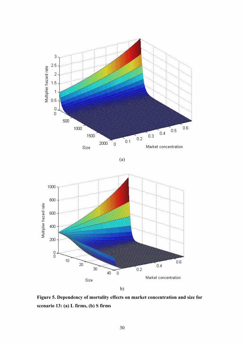
size under any scenario (Figure 5). These findings allow for two possibilities for the
case of increasing market concentration: either the mortality hazard increases slower
for the largest S firms than for L firms (Figure 6a), or the mortality hazard decreases
for the largest S firms whilst increases for all L firms irrespective of their size (Figure
6b).
[INSERT FIGURE 5 ABOUT HERE]
[INSERT FIGURE 6 ABOUT HERE]
Outcome 4. As market concentration increases, either (i) large S firms’ mortality
hazard decreases whilst that of L firms’ does increase or (ii) S firms’ mortality hazard
increases at a slower pace than that of L firms; (iii) the smallest S firms’ mortality
hazard always increases with concentration.
So dual market structure may also develop when increasing concentration raises S
firms’ hazard less than that of L firms. This outcome also indicates having an
endogenous minimal scale of production as an emergent property in our simulation
model: the very small players disappear. Small niche players falling below this
minimum scale cannot benefit from the space release induced by increasing
concentration. This indicates that the dual structure is developed by having large and
small (but not extremely small) firms.
Outcome 4 reveals that size effects operate differently on L and S firms. For L firms,
increasing size weakens the intensity of the concentration-related mortality effect;
however, the effect always stays increasing. For S firms, concentration might either
increase or decrease mortality. The broad range of size-related simulation outcomes
we have studied reveals that two types of partitioning, a weak and a strong one, can

17
emerge:8 as concentration rises, either L firms and S firms experience increasing and
decreasing mortality (strong partitioning), respectively, or both experience increasing
mortality, with S firms’ chances deteriorating at a slower pace (weak partitioning).
Regression results
As explained above, our OLS regression analysis takes the simulation model’s
parameters as independent variables out of 3,240 observations. In 17 observations, the
market has become extinct long before the end of the simulation’s time horizon. Our
four dependent variables were, again, average market concentration (Gini), L and S
firm density average over the last 500 time periods, and space release. The last effect
is proxied with L firm space contraction (Lcontr), the difference between maximum
and average space occupied by L firms in the last 500 time periods.
[INSERT TABLE 2 ABOUT HERE]
Our estimates are presented in Table 2.9 Market concentration was found to be
negatively correlated with the small sunk cost parameter QS and product dissimilarity
γ. This is in line with expectations, since increasing S firm scale advantages and
distance-related effects both lower the scale advantage of L firms.
As expected, L firm space contraction (Lcontr) is larger when Qs is larger, because
increasing S firm scale decreases the competitive advantage of L firms. Our
interpretation is that L firm space contraction is partially due to their direct
competition with S firms. This also suggests that L-firm’s space release in the
peripheries is not necessarily triggered by increasing market concentration, as quite a
few earlier studies observed in industries with a generalist-specialist dual structure [2,
13]. Here, our generic L-S firm model identifies broader conditions under which dual
structure can occur. We found a positive correlation between L firms’ endowment (E)
8 This finding resembles to the strong and weak patterns of partitioning observed in the dual-market study of Boone et al (2000) on Dutch auditing firms. 9 The minor non-normality of the residuals is not relevant as we have a large number of observations. In order to deal with heteroskedasticity, we ran our regression with robust standard errors whilst iteratively computing weighted least squares. The results were quite similar. Here, we only report the OLS estimates.
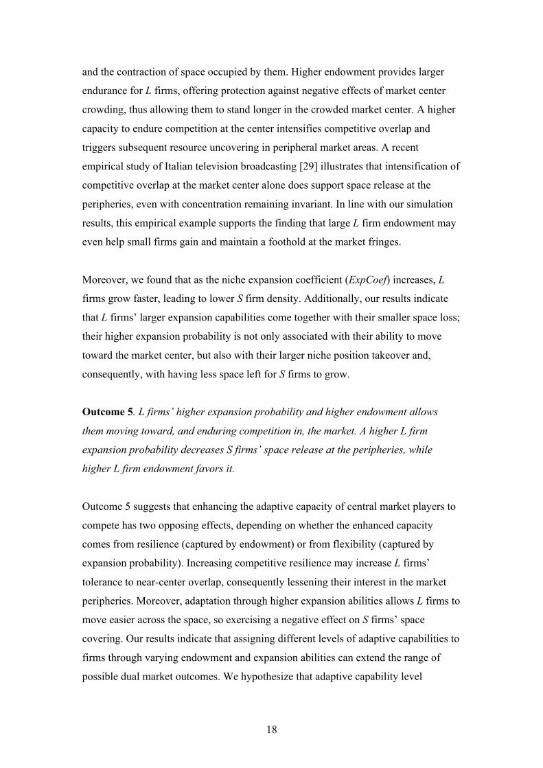
18
and the contraction of space occupied by them. Higher endowment provides larger
endurance for L firms, offering protection against negative effects of market center
crowding, thus allowing them to stand longer in the crowded market center. A higher
capacity to endure competition at the center intensifies competitive overlap and
triggers subsequent resource uncovering in peripheral market areas. A recent
empirical study of Italian television broadcasting [29] illustrates that intensification of
competitive overlap at the market center alone does support space release at the
peripheries, even with concentration remaining invariant. In line with our simulation
results, this empirical example supports the finding that large L firm endowment may
even help small firms gain and maintain a foothold at the market fringes.
Moreover, we found that as the niche expansion coefficient (ExpCoef) increases, L
firms grow faster, leading to lower S firm density. Additionally, our results indicate
that L firms’ larger expansion capabilities come together with their smaller space loss;
their higher expansion probability is not only associated with their ability to move
toward the market center, but also with their larger niche position takeover and,
consequently, with having less space left for S firms to grow.
Outcome 5. L firms’ higher expansion probability and higher endowment allows
them moving toward, and enduring competition in, the market. A higher L firm
expansion probability decreases S firms’ space release at the peripheries, while
higher L firm endowment favors it.
Outcome 5 suggests that enhancing the adaptive capacity of central market players to
compete has two opposing effects, depending on whether the enhanced capacity
comes from resilience (captured by endowment) or from flexibility (captured by
expansion probability). Increasing competitive resilience may increase L firms’
tolerance to near-center overlap, consequently lessening their interest in the market
peripheries. Moreover, adaptation through higher expansion abilities allows L firms to
move easier across the space, so exercising a negative effect on S firms’ space
covering. Our results indicate that assigning different levels of adaptive capabilities to
firms through varying endowment and expansion abilities can extend the range of
possible dual market outcomes. We hypothesize that adaptive capability level

19
differences between firms can weaken or reinforce partitioning outcomes in a broad
range of industries.
5. Discussion and conclusions
Our simulation results demonstrate that the set of large (typically generalist) firms to a
large extent coincides with the set of large sunk cost firms when the microeconomic
conditions adopted by our model are combined with a market center-periphery
distinction. Several of our simulation settings yielded dual market outcomes that are
similar to those predicted by other dual market approaches. This is, very likely, a
consequence of the resemblance of our model assumptions to assumptions of these
other theories. For example, our firms are characterized by a low/high sunk cost
distinction (just as at [1]) interacting in a market with a unimodal demand landscape
(just as at [2, 12, 29]). But the simulations also reveal aspects of dual market
formation, which, according to our knowledge, have not yet been addressed by other
theories. Below, we begin with the commonalities. This is followed by a summary
and interpretation of those findings that provide new insights on the causes and ways
of dual market formation.
Our results corroborating extant knowledge are as follows. Market concentration,
measured with the Gini index, increases mortality for all firms, large and small alike
(outcome 3). This is line with IO’s argument as to the entry barrier and market power
effect, as well as with main effect results from empirical market partitioning studies
(like the one of [28] on the dual market structure of the Dutch auditing industry). We
found space release at market peripheries with scale-based competition (outcome 2)
and with subsequent large firm shake-out at the market center. This finding shows a
clear analogy to documented cases of dual structure formation with center and
peripheral market players [2] (outcome 1). Even with a modest space release in place,
small S firms experience decreasing mortality rates with rising market concentration,
while large L firms’ mortality hazard increases in the meantime (outcome 4). Distance
to the center is a determinant of the mortality hazard (outcome 3). Also in line with
extant knowledge, we found that a noticeable level of firm heterogeneity – measured
20
in terms of sunk cost magnitudes in our case – is necessary to generate a center-
periphery market partitioning (cf. [16]).
The next findings reflect new insights that add to the extant literature on dual market
formation in particular, and to theories of market dynamics in general. The first
concerns the role of price mechanisms in market partitioning processes. From the very
beginning [2], resource-partitioning theory has focused on markets where price was
not the central aspect for customers (like in case of newspapers and microbreweries)
or where price effects are suppressed by other aspects like reputation or the bundling
of the offerings (such as in case of auditing services). We have demonstrated that a
dual market structure with center-periphery partitioning can well occur when agents
are sensitive to price.
Second, the effect of concentration on firm type (L and S firms) is moderated by a size
effect. We found that that there is an emergent (endogenous) minimum scale of
production that allows S firms to confront the negative effects of market concentration
and their distance to the market center as well (outcome 4). Size effects can establish
a concentration-dependent mortality threshold. Thus, the smallest S firms might
though avoid head-on competition with market-center players, but still might
succumb to other, somewhat larger, S firms.
Third, we found a temporally non-monotonic space release effect (outcome 2). L
firms may first move out from the center in order to lessen competition, so occupying
rather more than less (semi-)periphery positions. This happens because large sunk
cost L firms might not yet operate close to their full scale potentials; their ‘efficiency
slack’ can be used up to counterbalance scope diseconomies, and to expand, in the
early consolidation phase. Occasionally, L firms may even take over more space than
had been released. Later, when shake-out frees up additional affluent center demand
that survivor L firms can efficiently capture, the relative advantages of aiming at
scarcer periphery demand lessen, while L firms’ scope diseconomies at the peripheries
remain the same. At this mature phase, we found the space occupied by L firms
contracting. The bottom line is that scale-based competition at the market center,
alone, might not be enough to generate space release. Moreover, L firms may operate
below their optimal scale at the time increasing concentration appears, so that space
21
release might just partially emerge. Then, space gains, if occur, come at the expense
of L firms failing because of the pressure of those S firms that managed to reach a
certain size. Again, size effects per firm type operate in such a subtle way that while L
firms do not get any benefit from increasing market concentration, some larger S
firms do experience mortality hazard decline.
Fourth, enhanced adaptive capabilities of L firms (either through endowment or
increased expansion chances) have effects on resource release (outcome 5). The
magnitude of these capabilities (relative to each other) positively or negatively affects
resource release. Previously, [5] had claimed that the nature and degree of (scale and)
scope economies are key in understanding the precise equilibrium market structure
outcomes. Here, we add that the interplay between market-level selection forces and
firm-level adaptive capabilities we have introduced to our model gives room for the
emergence of a large number of new dual market outcomes.
Finally, we found connections to some other domains of market dynamics research.
The L / S firm distinction allows connecting our framework to research on the
efficiency / efficacy duality [30] and the first-mover / efficient producer dilemma [31,
32]. Concerning the first, newcomers to the market may be efficacious (effective) but
not efficient. They are efficacious in the sense of matching the environment – that is,
in identifying some attractive positions with positive demand to which these firms can
align their niche centers. Firms also gradually approach efficiency as they gain
experience through competition [33, 34]. However, such environmental matching
becomes more complex when a firm grows, and has to comply with multiple niches
and the associated matching requirements – a complexity that can be counterbalanced
with L firms’ positive scale advantages. We observed that efficient producers tend to
become the L firms in the market. Some other firms take an effective first-mover
approach, since they happen to adapt quickly to the identified market spot and start
making profits from the moment they step in. The long-term efficient producers have
higher sunk costs, have a scale-based strategy and need more time to reach an
operational point before generating positive returns.
The new findings broaden the set of conditions for which dual market structures can
be expected, and hence generalize the theory of market partitioning: (i) firms can

22
differentiate in their degree of scale advantage through their level of production
capacity (sunk costs); (ii) every firm faces a balance between scale and scope
economies; (iii) this balance depends on both the firms’ cost structure and their
location in the unimodal resource space; and (iv) firms can make use of their scale
advantage through price competition.
Computer simulation results are dependent on model architecture and
parameterization; so their findings do not prove, but rather may corroborate
hypothesized tendencies[35]. Our findings on new aspects of dual market structure
emergence indicate the possibility of such outcomes [15]. It is up to subsequent
empirical investigations to identify these, or similar, outcomes in real-world markets.

23
References
[1] Sutton, J. 1991. Sunk costs and market structure. Cambridge, MA: MIT Press. [2] Carroll, G. R. 1985. Concentration and specialization: Dynamics of niche width in populations of organizations. American Journal of Sociology, 90: 1262-1283. [3] Carroll, G. R., Dobrev, S., & Swaminathan, A. 2002. Organizational processes of resource partitioning. Research in Organizational Behavior, 24: 1-40. [4] Boone, C., & van Witteloostuijn, A. 2004. A unified theory of market partitioning: an integration of resource-partitioning and sunk cost theories. Industrial and Corporate Change, 13: 701-725. [5] van Witteloostuijn, A., & Boone, C. 2006. A resource-based theory of market structure and organizational form. Academy of Management Review, 31: 409-426. [6] Boone, C., & van Witteloostuijn, A. 1995. Industrial organization and organizational ecology: The potentials for cross-fertilization. Organization Studies, 16: 265-298. [7] Tirole, J. 1988. The theory of industrial organization. Cambridge, MA: The MIT Press. [8] Hotelling, H. 1929. Stability and competition. Economic Journal, 39: 41-57. [9] Lancaster, K. J. 1966. A new approach to consumer theory. Journal of Political Economy, 74: 132-157. [10] Liu, M. 2011. Market partitioning, organizational identity and geography: Empirical and simulation evidence in the German electricity market after deregulation. Unpublished doctoral dissertation, University of Lugano. [11] Carroll, G. R., & Swaminathan, A. 2000. Why the microbrewery movement? Organizational dynamics of resource partitioning in the U.S. brewing industry. American Journal of Sociology, 106: 715-762. [12] Boone, C., van Witteloostuijn, A., & Carroll, G. R. 2002. Resource distributions and market partitioning: Dutch daily newspapers, 1968 to 1994. American Sociological Review, 67: 408-431. [13] Boone, C., Carroll, G. R., & van Witteloostuijn, A. 2004. Size, differentiation and the performance of Dutch daily newspapers. Industrial and Corporate Change, 13: 117-148. [14] Péli, G., & Nooteboom, B. 1999. Market partitioning and the geometry of the resource space. American Journal of Sociology, 104: 1132-1153. [15] Burton, R. M., & Obel, B. 1995. The validity of computational models in organization science: From model realism to purpose of the model. Computational and Mathematical Organization Theory, 1: 57-71.

24
[16] García-Díaz, C., & van Witteloostuijn, A. 2011. Firm entry diversity, resource space heterogeneity and market structure. Lecture Notes in Economics and Mathematical Systems, 652: 153-164. Berlin Heidelberg: Springer. [17] McPherson, M. 2003. A Blau space primer: prolegomenon to an ecology of affiliation. Industrial and Corporate Change, 13(1): 263–280. [18] Hannan, M. T. 2005. Ecologies of organizations: Diversity and identity. Journal of Economic Perspectives, 19: 51-70. [19] Adner, R., & Levinthal, D. A. 2001. “Demand heterogeneity and technology evolution: Implications for product and process innovation.” Management Science, 47: 611-628. [20] Le Mens, G., Hannan, M. T., & Pólos, L. 2011. Founding conditions, learning and organizational life chances: Age dependence revisited. Administrative Science Quarterly, 56: 95-126. [21] Simon, H. A. 1957. Models of man: Social and rational. New York: John Wiley. [22] Cyert, R. M., & March, J. M. 1963. A behavioral theory of the firm. Englewood Cliffs, NJ: Prentice Hall. [23] White, H. C. 1981. Where do markets come from? American Journal of Sociology, 87: 517-547. [24] Kleijnen, J. P. C. 2007. Design and analysis of simulation experiments. Berlin: Springer. [25] Barron, D. N. 1999. The Structuring of organizational populations. American Sociological Review, 64: 421-445. [26] Barron, D. N. 2001. Simulating the dynamics of organizational populations. In Lomi, A. & Larsen, E. R (Eds.) Dynamics of organizations: Computational modeling and organization theories, pp. 209-242. Cambridge, MA: MIT Press. [27] Swaminathan, A. 1995. The proliferation of specialist organizations in the American wine industry, 1941-1990. Administrative Science Quarterly, 40: 653-680. [28] Boone, C., Bröcheler, V., & Carroll, G. R. 2000. Custom service: Application and tests of resource-partitioning theory among Dutch auditing firms from 1896 to 1992. Organization Studies, 21: 355-381. [29] Reis, S., Negro, G., Sorenson, O., Perreti, F., Lomi, A. (2012). Resource partitioning revisited: evidence from Italian television broadcasting. Industrial and Corporate Change, 22: 459-487. [30] Drucker, P. F. 2006. What executives should remember. Harvard Business Review, 84: 144-152.

25
[31] Lieberman,M. B. & Montgomery, D. B. 1988. First-mover advantages. Strategic Management Journal, 9: 41-58. [32] Péli, G., & Masuch, M. 1997. The logic of propagation strategies: Axiomatizing a fragment of organizational ecology in first-order logic. Organization Science, 8: 310-331. [33] Barnett, W. P. 2008. The red queen among organizations: How competitiveness evolves. Princeton, NJ: Princeton University Press. [34] Péli, G. 2009. Fit by founding, fit by adjustment: Reconciling conflicting organization theories with logical formalization Academy of Management Review, 34(2): 343-360. [35] Popper, K. R. 1959. The logic of scientific discovery (translation of Logik der forschung, 1935). London: Hutchinson. [36] Hannan, M. T., Carroll, G. R., & Pólos, L. 2003. The organizational niche. Sociological Theory, 21: 309-340. [37] Hannan, M. T., Pólos, L., & Carroll, G. R. 2007. Logics of organization theory: Audiences, codes, and ecologies. Princeton, NJ: Princeton University Press.

26
Figure 1. Correspondence between the three firm typologies
As time passes surviving L firms tend to be large and have a broad niche, while
surviving S firms tend to be small and have a narrow niche.
Most large-sized firms of the model belong here
Broad niche (generalist firms)
Large sunk costs (L firms)
Large-sized firms

27
(a) (b)
(c)
Figure 2. Average model behavior in Scenario 6 (shadowed regions correspond
to confidence intervals)

28
Figure 3. Size distribution per firm type (aggregated data on all simulations for
this scenario)

29
(a)
(b)
Figure 4. L-firm space occupancy over time (shadowed regions correspond to
confidence intervals)
30
(a)
b)
Figure 5. Dependency of mortality effects on market concentration and size for
scenario 13: (a) L firms, (b) S firms

31
(a)
(b)
Figure 6. Mortality effects with increasing concentration per firm type:
Scenarios 1 (a) and 5 (b), respectively

32
Size Gini DC Type
Sc. Coef. % Sig. Std .Dev Coef. % Sig. Std .Dev Coef. % Sig. Std .Dev Coef. % Sig. Std .Dev
1 -0.17 100% 0.04 4.52 100% 2.11 1.23 83% 1.02 3.88 100% 0.33
2 -0.20 100% 0.05 7.70 100% 1.53 0.69 57% 1.05 4.35 100% 0.18
3 -0.15 100% 0.03 5.39 100% 3.31 0.62 70% 0.82 3.96 100% 0.22
4 -0.18 100% 0.06 1.63 87% 3.64 0.02 30% 0.48 4.06 100% 0.21
5 -0.12 100% 0.03 6.01 97% 2.24 0.65 80% 0.88 4.01 100% 0.26
6 -0.20 100% 0.05 2.46 97% 1.46 0.91 93% 0.82 3.82 100% 0.34
7 -0.17 100% 0.03 3.21 100% 1.20 0.96 93% 0.92 3.89 100% 0.27
8 -0.17 100% 0.03 4.09 100% 1.38 1.18 90% 0.51 3.84 100% 0.24
9 -0.06 100% 0.02 1.10 93% 0.34 0.28 40% 0.27 1.72 100% 0.02
10 -0.16 100% 0.03 2.28 100% 0.88 0.78 93% 0.36 4.11 100% 0.23
11 -0.20 100% 0.03 2.60 100% 0.89 0.75 87% 0.71 3.90 100% 0.21
12 -0.16 100% 0.04 4.18 100% 1.09 1.44 97% 0.69 3.87 100% 0.25
13 -0.16 100% 0.04 4.85 100% 1.66 1.44 90% 1.51 4.02 100% 0.26
Table 1. Survival analysis coefficients

33
Independent variables Concentration
(Gini) index
L density S density L space
contraction
QS
Small sunk
cost
parameter -.0175831* -.1431061* 2.774796*
1.363785*
(.0002214) (.0045447) (.0448818) (.0217619)
γ Product
dissimilarity -.0025169* .0045806 .5720272*
.1815882*
(.0001565) (.0031975) (.0340542) (.0149023)
ϕ Markup
factor .1163989* -1.44986* 76.54684*
9.791984*
(.0155546) (.3160434) (3.394657) (1.464913)
ExpCoef Expansion
coefficient 3.238009* 8.51728* -263.9791* -121.3129*
(.1568174) (3.169922) (34.50324) (14.7435)
E Endowment .00345* 1.250871* .0937271 .6340934*
(.0002614) (.0061466) (.0563541) (.0244667)
X Entry rate .0007879* 5.255838* 7.353022* 3.898299*
(.0025293) (.0516949) (.5532305) (.2395199)
Intercept .8440625* -9.539741* -106.2712* -39.89156*
(.0233112) (.4662876) (5.094417) (2.274647)
Number of
observations
3223 3223 3223 3223
F(6, 3126) 1125.17 8786.44 801.88 784.76
R² 0.6845 0.9545 0.5640 0.6199
Root MSE 0.07178 1.4674 15.711 6.8014
Robust standard errors in parenthesis; * p < 0.05.
Table 2. Regression results

34
Materials and Methods
Extended conceptual model description
A.1 The resource space and location specification at entry
The resource space corresponds to a unimodal distribution of consumers along a set of taste preferences
of size N. Each taste preference has a number bk of consumers, k = 1,2, …, N. The resource space is set
according to a beta distribution with parameters α*=β*=η. In order to get a unimodal representation
we use η = 3 and N = 100. Firms enter the market at a constant rate x per time period provided that the
space is not completely occupied; otherwise (i.e., when the market is fully saturated) there is no entry.
All the simulation runs are performed using a total demand of ∑kbk = 5500 consumers. Firms that enter
the market pick up their initial location according to the probability distribution of non-served
consumers, ρ t, which is given by:
NkbCBP
bCBPN
iiti
ktktk ,...,2,1,
)1(
)1(
11,
1,, =∀
−
−=
∑=
−
−ρ , (A1)
where CBPk,t-1 represents the active consumer base percentage at position k at time t-1. Since at the
beginning of the simulation (t = 0) there is no active consumer base, then ρk,0 = bk/∑bi.
A.2 Firm’s cost structure
Firms have a two-piece cost function. One piece relates to the production costs CiPROD,t, and the other
one accounts for the niche-width costs, CiNW,t,:
itNW
itPROD
it CQCQC ,, )()( += . (A2)
Production levels Q are quantified through a Cobb-Douglas function:
βαtiiti VFQ ,, = . (A3)
Coefficients α and β correspond to production volume elasticities with respect to production factors F
and V (that is, α = (∂Q/∂F)(F/Q) and β = (∂Q/∂V)(F/Q)). Firms derive their production costs, CiPROD,t,
from a long-run average cost curve, LRAC, of the whole industry. The LRAC curve is the envelope of
the most efficient production possibilities in the industry. We make α + β > 1 in order to reflect a
downward-sloping LRAC and positive scale economies. Production costs for the firm are calculated
according to the usage of production factors amounts F and V that the firm needs to produce quantity
Q. That is, assuming that production factor prices are WF and WV, respectively, the LRAC curve is
calculated by solving the following optimization problem:
βαtiiti
iViF
VFQtsVWFW
,,..min
=
+. (A4)
Parameters WV, WF, α and β are set in order to obtain a (normalized) unit cost of 1 when Q = ∑ibi (WV
= 4.15, WF = 2WV, α = β = 0.7). The production cost of every firm i, CiPROD,t, is also computed through
Equation (A4), but then assuming that the firm has a fixed usage of factor F, independent from

35
production levels (that is, WFFi represents firm’s fixed costs). Firms may have two different
alternatives to define the usage of factor F: a large (L) and a small one (S). These two options define
the two different firm types in the model. Each one of the two possible values of F is set according to
the quantity Q at which the firm’s cost curve and the LRAC intersect. The model assumes that the large
fixed cost indicator, QL, is set at least at half of the total market demand, QL ≥ ∑ibi/2, while the small
sunk cost value, QS, varies from quantities as low as 5, QS ≥ 5. The baseline model uses QL = ∑ibi/2 and
QS = 10. However, model’s behavior is also inspected under different “scale distances” (QL - QS). An
entrant has equal probability to select either firm type.
Niche-width costs represent the negative effect of covering a market with a large scope of consumer
preferences. That is, a firm finds it more expensive to cover a highly diverse consumer-preference
market than a homogenous one. Niche-width costs are defined as a function of the upper and lower
limits of firm i’s niche, and a proportionality constant NWC:
lti
uti
itNW wwNWCC ,,, −= , (A5)
where . represents the (Euclidean) distance between the two niche limits, and wli,t and wu
i,t represent
the firm’s lower and upper niche limits. Firm i’s niche center is then defined as
lti
lti
uti
it wwwnc ,,, 2/ +−= .
A.3 Consumer behavior
Each consumer buys only once every time period. Assuming that the selected firm has still enough
produced units to cover demand, and that Sk,t represents the set of firms that have an offer at position k,
a consumer evaluates the offerings at his or her location k. The consumer buys from the firm that offers
the lowest compound cost (price plus product dissimilarity) from the set of options {Uik,t} (i.e.,
considering all the i-th firms that belong to the set Sk,t):
{ }⎪⎭
⎪⎬⎫
⎪⎩
⎪⎨⎧
−
−+
∈=
∈=
)1(minmin
,,
,
*, N
kncP
SiU
SiU
iti
ttk
itk
tktk γ , (A6)
where Pit is the firm i’s price at time t, and γ is a constant that quantifies the effect of distant offerings
in the space from the firm’s niche center (product dissimilarity). The distance-related effect is
normalized over the maximum possible Euclidean distance in the model, N - 1. In case that the selected
firm does not have enough produced units to satisfy a consumer, the consumer decides to buy from the
second cheapest alternative, and so on. To avoid any synchronization artifact, order positions for the
buying process are randomly permuted every time period.
The reader might ask why apparently the distance effect is counted twice: firms have a negative scope
effect through the niche-width cost, but also are penalized through the product dissimilarity effect. The
two settings {γ > 0, NWC = 0} and {γ > 0, NWC > 0} produce rather similar results: Both revealed in
the long run that L firms basically take over the center while S firms locate at periphery. This means

36
that the inclusion of NWC does not influence the scale-based selection process of the model. However,
only the setting {γ > 0, NWC > 0} revealed a sharp niche-width difference between firms located at the
periphery and those located at the center. Therefore, we adopt such a setting {γ > 0, NWC > 0}, since it
resembles more precisely what resource-partitioning theory argues: Location in the space is related to
the degree of niche-width differentiation (generalism / specialism).
For the sake of simplicity, we do not use demand functions, but define a limit price value for firm
operations. The maximum price a consumer is willing to pay corresponds to a opportunity cost of the
smallest efficient firm in the industry Pmax = (1+ϕ)LRAC⏐Q=1. This implies that the only reason a
consumer would buy from a larger firm is that such a firm is more cost-efficient than the smallest
possible firm in the industry (i.e., the firm’s “scale” Q is located rightward along the LRAC curve).
That said, consumers are allowed to bear a maximum cost Uo, so that Uik,t ≤ Uo = Pmax. The amount Uo
defines a cost-related participation constraint for consumers. In general, if the consumer chooses to buy
from a firm i* whose niche center does not coincide with the consumer’s preference k, the price Pi*t has
to comply with
)1(max*
−
−−≤
N
kncPP
iti
t γ . (A7)
In order to reflect scale advantages, firms use a markup price over average costs (i.e., (1+ϕ)C(Q)/Q),
provided that the markup price complies with Equation (A7). Coefficient ϕ may range between 0 and
1.
We calibrated coefficients NWC and γ following these steps: (i) Since we assume that L firms are more
efficient than S firms, we also assume that in absence of distance-related dissimilarity (γ = 0), a fully-
expanded L firm should be able to outcompete any S firm. Experimentation with the model reveals that,
to comply with that, the maximum value that the maximum vale the NWC coefficient can take is 195;
(ii) with NWC = 195, the value range of coefficient γ was specified by assuming that the fundamental
niche of an L firm (i.e., the space the firm would occupy in absence of any competition; see[36, 37])
should oscillate between half and two-thirds of the total resource space (that is, γ ∈ [50, 70]).
A.4 Entry price setup
Firms enter at one single position in the space. As seen in Equation (A1), we assume that firms search
for a competitor-free foothold to enter the market. Firms pay attention to residual demands – the
amount of non-served consumers – at different points in the resource space. From Equation (A1), we
observe that the probability they step in a given location increases with the size of the residual demand
spot. If the selected position for entry is position k, the firm considers a potential production quantity Q
= (1 - CBPk)bk, which corresponds to the residual demand. The firm fixes a unit price that corresponds
to min{Pmax, (1 + ϕ)C(Q)/Q}.

37
L firms may need some time to grow and reach an operation point that allows them to sustain positive
profits. S firms are able to make profits at the time they enter the market. L firms have negative profits
until they reach a minimal operational point. Thus, we assume that L firms have an initial endowment.
Endowment is implemented as a number E of periods for which a firm can survive in case of no sales
(that is, covering fixed costs for E time periods). For the baseline model, E = 12, but other values are
explored in order to investigate implications on the model’s results.
A.5 Firm expansion
There are two possible ways for a firm to expand: vertical and horizontal. The firm uses an adaptive
“rule of thumb”, based on the latest information of the market, to assess if expansion is worth the
investment. Being the expansion either vertical or horizontal, the firm first defines a target quantity in
terms of the latest observed prices and costs. Based on such a quantity, the firm computes incremental
profits and decides whether or not expansion is worth the investment.
(i) Vertical expansion refers to a niche production quantity adjustment. At time t, firm i makes
production adjustments for the next round and targets the residual demand ΔQv,t+1 − the amount of non-
served consumers − in their current niche Hi,t, so that ΔQv,t+1 = ∑k∈Hi,t(1-CBPk,t)bk. Then, if Qt represents
firm i’s latest sold quantity, the firm evaluates whether incremental revenues surpass incremental costs.
If that is the case, the firm expands. Incremental costs are computed as Ci(Qt + ΔQv,t+1) –Ci(Qt).
Incremental revenues are computed as Pi*(Qt+ΔQv,t+1) - PitQt, where Pi* is calculated as follows:
⎪⎭
⎪⎬⎫
⎪⎩
⎪⎨⎧
Δ++−
−−= + )()1(,
)1(min 1,
,max
*tvt
lti
iti QQCNwnc
PP ϕγ . (A8)
That is, firms use a markup price as long as it does not exceeds the maximum allowed price according
to the width of the firm’s current niche (see Equation (A8)).
(ii) Horizontal expansion refers to niche expansion. It also establishes a target quantity ΔQuh,t+1 and
ΔQlh,t+1 on either side of the current firm’s niche (upper and lower limits), respectively. The firm
decides to expand toward the most attractive direction – that is, to the position where incremental
profits are larger – in a similar fashion shown for vertical expansion. Firms do not always expand, so
that expansion is controlled by an expansion probability, ExpCoef, at every time period. Values for the
coefficient ExpCoef were jointly selected along with the time-horizon span over which we expected to
see a convergence of market concentration and firm density. Since we run the model for 2000 time
periods, our criteria is that an L firm should have enough time to fully expand to its fundamental niche,
even if it enter the market at a mature state (> 1000 time periods). Values were chosen between 0.03
and 0.05. This coefficient might be also related to the firm’s degree of inertia. Along with the results
reported here, it is worth mentioning that our simulation trials confirmed a location-related selection
process – L firms taking over the center and S firms dominating the periphery – even in absence of any
inertia effects (i.e., ExpCoef = 1).
38
In the case a firm decides to expand, it evaluates in which direction to go. The quantities ΔQuh,t+1 and
ΔQlh,t+1 are set according to the same set of rules. Let us assume that firm i attempts expansion to the
position adjacent to its upper niche limit, z. If the targeted position z is empty, then ΔQuh,t+1 = bz. If
some firms are already at position z, then the expanding firm i estimates ΔQuh,t+1 by taking into account
the rival’s costs Ujz,t, and rivals’ latest sold quantities, at position z, which firm i assumes to be the best
estimates of their next time-period quantities. Then, the offered costs are compared and ranked, and the
quantity ΔQuh,t+1 is subsequently extracted according to the relative rank the firm gets in comparison
with the rivals’ costs. An example of how this is carried out follows next. Let us assume that the
location of interest has a total demand of ten consumers, and the compound costs at that position from
two different firms are U(A) = 10 and U(B) = 15 with captured demands Q(A) = 7 and Q(B) = 3. If firm
C attempts to enter that position, and assuming that U(C) = 12, the ascendant cost ranking will place
firms in the following order: A, C, and B. Firm C estimates that A will keep its last demand in the next
round (i.e., Q(A) = 7), since A still has the cheapest offer. But now, given that C has a better offer than
B, C will steal B’s demand and estimate that in the next round Q´(C) = 3 and Q´(B) = 0. Once the target
quantity has been established for z, the firm calculates its potential incremental profits by taking into
account (i) the resulting total costs with the added target, (ii) the resulting price, including the new
distance compensation )1/(),( −−+ Nznci ztHiγ , where nciHi,t+z is the new niche center that would
result if z is included in firm i’s niche, Hi,t, and (ii) the firm’s latest price and costs. The firm then
computes incremental profits and performs the same calculation when expansion is attempted to the
cell adjacent to the lower limit. After comparing the two incremental profits, the firm decides to expand
toward the position that reveals the highest value, if any.
A.6. Analysis
We study the effect on hazard rates according to different representative scenarios, which are set
according to variations in small sunk cost investment (QS), product dissimilarity coefficient (γ),
endowment (E), entry rate (X), markup value (ϕ) and expansion probability (ExpCoef). The scenarios
correspond to a model with mid-range parameters (scenario 1), variations in the small sunk cost
investment (scenarios 2, 3 and 4), markup (scenarios 5 and 6), product dissimilarity (scenarios 7 and 8),
endowment (models 9 and 10), probability of expansion (scenarios 11 and 12) and entry rate (scenario
13). Every scenario is run for 2000 time periods. Within every scenario, we also studied the behavior of
main time-evolving variables of interest (i.e., market concentration, per-type density and per-type total
covered space). Every scenario is run 30 times in order to guarantee the normality assumption of
confidence intervals of such variables. We find survival analysis estimators for each realization of the
30 x 13 = 390 simulations. See Table A1 for details.

39
Parameter Definition 1 2 3 4 5 6 7 8 9 10 11 12 13
QSS Small sunk
cost
10 5 15 20 10 10 10 10 10 10 10 10 10
ϕ Markup 0.2 0.2 0.2 0.2 0.1 0.3 0.2 0.2 0.2 0.2 0.2 0.2 0.2
γ Product
dissimilarity
60 60 60 60 60 60 50 70 60 60 60 60 60
E Endowment 12 12 12 12 12 12 12 12 6 18 12 12 12
ExpCoef Expansion
probability
0.04 0.04 0.04 0.04 0.04 0.04 0.04 0.04 0.04 0.04 0.03 0.05 0.04
x Entry rate 3 3 3 3 3 3 3 3 3 3 3 3 2
Table A1. Parameter values for model dynamics analysis
The second analysis consists of exploring effects in four specified outcomes: market concentration, L
firm density, S firm density, and L firm space contraction. Space contraction is evaluated as the
difference between the peak space occupation and the average occupation at the final time steps of the
simulation. Effects are explored with respect to variations in the simulation key parameters: small sunk
cost (QS), product dissimilarity (γ), markup (ϕ), endowment (E), Expansion probability (ExpCoef), and
entry rate (x). Using the selected values presented in Table A2, we get 4 x 34 x 2 = 648 combinations
for the above-mentioned parameters, respectively. We build an OLS regression model using the below-
mentioned parameters as independent variables, using the earlier mentioned four outcomes of interest
Parameter Definition Selected values
QSS Small sunk cost parameter 5, 10, 15, 20
γ Product dissimilarity 50, 60, 70
ϕ Markup factor 0.1, 0.2, 0.3
ExpCoef Expansion coefficient 0.03, 0.04, 0.05
E Endowment 6, 12, 18
x Entry rate 2,3
Table A2. Parameter values for OLS analysis
Every parameter combination was replicated m = 5 times. Thus, the total number of observations in this
analysis is 648 x 5 = 3240. To guarantee more precise effects on convergence conditions, we run each
simulation for 5000 time periods, and take averages on the last 500 periods on the key outcome
variables (i.e., the last 10% fraction of the total simulation time).