Embed Size (px)
Citation preview

Micro Hydroelectric Reservoir Storage Use for creating an
Uninterrupted Power Supply; Production case Studies in
Iceland
Huw Coverdale Jones
Faculty of Industrial Engineering, Mechanical
Engineering and Computer Science,
University of Iceland
2017
Table


Micro Hydroelectric Reservoir Use for creating and
Uninterrupted Power Supply; Production case Studies
in Iceland
Huw Coverdale Jones
60 ECTS thesis submitted in partial fulfilment of a
Magister Scientiarum degree in Environment and Natural Resources -
Renewable Energy - Energy Economics, Policy and Sustainability
Advisors
Rúnar Unnþórsson
Reynir Smári Atlason
Faculty Representative
Sæþór Ásgeirsson
Faculty of School of Industrial Engineering, Mechanical Engineering and
Computer Science
School of Engineering and Natural Sciences
University of Iceland
Reykjavik, August 2017


Micro Hydroelectric Reservoir Use for creating an Uninterrupted Power Supply; Production case Studies in Iceland.
Micro Hydro Reservoir Use for Uninterrupted Power Supply.
60 ECTS thesis submitted in partial fulfilment of a Magister Scientiarum degree in Environment and Natural Resources - Renewable Energy - Energy Economics, Policy and Sustainability.
Copyright © 2017 Huw Coverdale Jones
All rights reserved
Faculty of Industrial Engineering, Mechanical Engineering and Computer Science
School of Engineering and Natural Sciences
University of Iceland
School of Engineering and Natural Sciences
Hjarðarhagi 6
107, Reykjavik
Iceland
Telephone: 525 4000
Bibliographic information:
Jones, Huw Coverdale, 2017, Micro Hydroelectric Reservoir Storage Use for creating an Uninterrupted Power Supply; Production case Studies in Iceland, Master’s thesis, Faculty of Industrial Engineering. Mechanical Engineering and Computer Science, University of Iceland, pp. 101.
Printing: Háskolaprent
Reykjavik, Iceland, August,2017


Abstract
Micro hydroelectric installations are an established power generation system that have been
applied in Iceland previously. Combinations of hydroelectric storage and intermittent resources,
such as wind, are also an established method of creating a consistent supply with no power failure.
Furthermore, the problems of effectively storing electricity for future use are a key problem in the
establishment of an effective electrical system.
This research created a theoretical micro hydroelectric power plant, combined with a
downsized model of an existing wind turbine, and a theoretical hydroelectric reservoir for storage.
This research defines a micro hydropower plant as having 1MW installed capacity or less. This thesis
then tested the ability to maintain a considerable consistent output that outstretches the domestic
needs of an average household. The key aim of the research was to establish the effective storage
status of the reservoir itself. It was found to be key to the maintenance of the system’s consistent
generation, both for meeting domestic need, as well as maintaining a consistent and uninterrupted
generational output.
As Iceland generally doesn't lack domestic electrical supply, a series of production case
studies were tested against the consistent output of the micro hydroelectric installation. The
consistent electrical output was measured in terms of ability to support industrial and agricultural
scenarios. The micro generation system was found to be suited to powering hydrogen electrolysers,
small scale aquaponics farming systems, and a 1 to 2 rack data centre for personal use. These were
found to be heavily reliant on the reservoir to meet key power shortages across the yearly
generation period.


Útdráttur
Samfelld og jöfn orkuframleiðsla smávatnsaflsvirkjana með notkun uppistöðulóna;
tilviksathuganir á Íslandi.
Smáar vatnsaflsvirkjanir hafa verið í notkun á Íslandi til margra ára . Þær hafa verið notaðar einar
og sér og með uppistöðulónum. Tilgangur uppistöðulónanna hefur verið til að halda vatnsrennsli
stöðugu og þannig jafna raforkuframleiðsluna og koma í veg fyrir að framleiðslan stöðvist.
Vatnsaflsvirkjanir með uppistöðulónum hafa einnig verið notaðar í sama tilgangi samhliða óstöðugri
raforkuframleiðslu, s.s. með vindorku. Orkugeymsla, eins og með uppistöðulónum, er mikilvægur
hluti af raforkukerfum þar sem kröfur eru gerðar um samfellda og jafna orkuframleiðslu.
Í þessu rannsóknaverkefni var útbúið fræðileg líkan af smávatnsaflsvirkjun með uppistöðulóni
og líkanið tengt við aðlöguð raungögn frá vindtúrbínu. Smávatnsaflsvirkjanir – í þessari rannsókn –
eru virkjanir sem framleiða undir 1MW. Í verkefninu var geta líkansins til að framleiða raforku yfir
þarfir meðal heimilis og viðhalda henni. Meginmarkmið verkefnisins var að skoða og ákvarða
eiginleika uppistöðulónsins þannig að það fengist samfelld og jöfn orkuframleiðsla þó kerfið væri
tengt við vindtúrbínu.
Þar sem almennt er ekki er skortur á rafmagni til heimila á Íslandi, voru nokkrir
nýtingarmöguleikar á raforku frá smávirkjunum til framleiðslu skoðaðir. Miðað var við samfellda og
jafna raforkuframleiðslu sem nýta mætti bæði í iðnaði og landbúnaði. Niðurstöður eru að
raforkuframleiðsla frá smávatnsaflsvirkjunum hentar vel til að framleiða vetni með rafgreiningu,
reka smá aquaponics kerfi og lítil gagnaver til einkanota. Þessi kerfi eru mjög háð raforku og þarf
að nota uppistöðulón með smávirkjunum til að reka þau.


Dedication
This thesis is dedicated to Hanna Bedbur, for her emotional support, my parents, for all their
support, and the stand-up comedy scene of Reykjavik, for all their distraction during stressful
times.


Preface
This thesis was completed within the University of Iceland Faculty of Industrial Engineering,
Mechanical Engineering and Computer Science, between August 2016 and October 2017. It serves
as a 60 ECTs thesis for completion of a Magisters Scientiarum in Environment and Natural Resources
- Renewable Energy - Energy Economics, Policy and Sustainability.
During my studies, I have become concerned with the issue of energy storage systems
(hereafter ESS) to offset the intermittency of more renewable electricity sources. Specifically, I have
become interested in the use of water as a form of energy storage in Hydropower plants (hereafter
HPPs). I am specifically interested in is potential for some of these resources to complement each
other. The obvious example is the intermittency of wind power being offset by hydropower
installations in the areas, such as the current proposal at Hafið, Iceland (‘Búrfellslundur EN - Búrfell
Wind Farm’, n.d.). This paper will focus on a similar arrangement to build on possibilities for its
consistent electrical output, in combination with storage systems to ensure continued power
quality. Moreover, I became interested in the concept of small scale HPP usage in areas that exist
away from the major grid of their respective nations early in my studies. The issue of creating an
uninterrupted, storage-based, power supply that can act independently will be considered over the
course of this research.
The purpose of this thesis is to first establish the state of the art of storage systems for a
small scale. After this, the purpose is to explore the creation of independent uninterruptible power
supplies at small scales using suitable storage technologies. Finally, determining what else can be
achieved, beyond domestic supply, with these micro-scale power supplies will be the last aim of
this research.

xv
Table of Contents
Abstract .............................................................................................................. vii
Útdráttur .............................................................................................................. ix
Preface ............................................................................................................... xiv
Table of Contents ................................................................................................ xv
List of Figures ................................................................................................... xviii
List of Tables: ..................................................................................................... xix
Abbreviations ...................................................................................................... xx
Acknowledgements ............................................................................................ xxi
1 Introduction ..................................................................................................... 1
1.1 Contribution: ................................................................................................... 2
1.2 Research Problem and Questions: .................................................................. 3
1.3 Scope & Limitations: ....................................................................................... 4
2 Methods & Materials ........................................................................................ 6
2.1 Existing ESS System Literature Review Methodology:.................................... 6
2.2 Summary of Micro Hydro preparatory methods: ........................................... 7
2.3 Case Studies: ................................................................................................... 9
2.4 Economic Methodology: ............................................................................... 12
2.5 Data Used ...................................................................................................... 15
2.5.1 Load Data: ........................................................................................... 15
2.5.2 Supply Data ......................................................................................... 16
3 Storage Systems for Microgrids: An Assessment of literature ........................... 22
3.1 Existing Storage Technologies ...................................................................... 22
3.1.1 Description of Storage Processes ....................................................... 22
3.1.2 Mechanical Storage Technologies ...................................................... 22

xvi
3.1.3 Electrical Storage Technologies .......................................................... 24
3.1.4 Thermal Storage Technologies ........................................................... 25
3.1.5 Chemical Storage Technologies .......................................................... 27
3.2 Storage Comparison for Small-Scale or Micro-Grid Applications ................. 33
3.2.1 Scalability ............................................................................................ 34
3.2.2 Energy Density .................................................................................... 35
3.2.3 Efficiency ............................................................................................ 36
3.2.4 Storage Scale and Duration ................................................................ 37
3.2.5 Technological Maturity and Proven Status ........................................ 39
3.2.6 Costs ................................................................................................... 41
3.2.7 Life span .............................................................................................. 43
3.2.8 Other Restrictions............................................................................... 45
3.2.9 Discussion: Storage for Microgrids or Small-Scale Electricity
Generation .......................................................................................... 49
4 Existing Planning and Analysis Methods; Evaluation ........................................ 52
4.1 Area Analysis Method ................................................................................... 52
4.1.1 Method Description ........................................................................... 52
4.1.2 Method Test Application: ................................................................... 52
4.2 The Analytical Reservoir Sizing Method ....................................................... 56
4.2.1 Method Description ........................................................................... 56
4.2.2 Method Analysis ................................................................................. 57
4.3 The Electricity System Cascade Analysis: ...................................................... 60
4.3.1 Method Description: .......................................................................... 60
4.3.2 Method Analysis: ................................................................................ 62
4.4 HOMER.......................................................................................................... 64
4.4.1 Method Description ........................................................................... 64
4.4.2 Method Analysis ................................................................................. 65
5 Production Case Studies ................................................................................. 70
5.1 Grid Resale .................................................................................................... 70
5.2 Hydrogen Production and Storage: .............................................................. 71

xvii
5.3 Aluminium Smelting...................................................................................... 74
5.4 Aquaponics and Hydroponics ....................................................................... 75
5.5 Data Centres and Super Computers ............................................................. 78
6 Economic Summary ........................................................................................ 82
6.1 Grid Resale .................................................................................................... 82
6.2 Hydrogen Production and Storage ............................................................... 83
6.3 Aluminium Smelting...................................................................................... 84
6.4 Aquaponics and Hydroponics ....................................................................... 85
6.5 Data Centres and Super Computers ............................................................. 86
6.6 Economic Conclusion and Summary: ............................................................ 87
7 Conclusions and Discussion ............................................................................. 88
7.1 Sensitivity Study ............................................................................................ 88
7.2 Discussions .................................................................................................... 89
7.2.1 Case 1: Grid Resale ............................................................................. 89
7.2.2 Case 2: Hydrogen Production ............................................................. 90
7.2.3 Case 3: Aluminium Smelting .............................................................. 90
7.2.4 Case 4: Aquaponics and Hydroponics ................................................ 91
7.2.5 Case 5: Data Centres and Super Computers ...................................... 91
7.2.6 Legal Considerations ........................................................................... 92
7.3 Conclusions ................................................................................................... 93
References .......................................................................................................... 96

xviii
List of Figures
Figure 1. Load profile average displayed in HOMER. ................................................... 15
Figure 2. Yearly profile load displayed in HOMER. ....................................................... 16
Figure 3 Data equally redistributed across the year. ................................................... 16
Figure 4. Wind power generation based on original Burfell data. ............................... 17
Figure 5. Hydro generation at Geirlandsá. ................................................................... 18
Figure 6. HPP Generation profile based on new case study data. ............................... 18
Figure 7. Wind Generation based on case study data. ................................................ 19
Figure 8. Combined case study data generation profile. ............................................. 19
Figure 9. Outline of Combined Power System. ............................................................ 20
Figure 10. Geirlandsá river’s location, Kirkjubaejarklaustur displayed in google maps.
................................................................................................................. 53
Figure 11. Geirlandsá river, height potential annotated. ............................................ 54
Figure 12. Monthly litre load averages from original data. ......................................... 58
Figure 13. Data generated for methodological debugging. ......................................... 66
Figure 14. Turbine inputs in HOMER. ........................................................................... 66
Figure 15. System Architecture in HOMER. ................................................................. 67
Figure 16 Payback analysis for Grid Resale. ................................................................. 83
Figure 17 Payback Analysis for Hydrogen Production.4 .............................................. 84
Figure 18 Payback Analysis for Aluminium. ................................................................. 85
Figure 19 Payback Analysis for Aquaponics. ................................................................ 86
Figure 20 Payback analysis for the Data Centre. .......................................................... 87

xix
List of Tables:
Table 1 Glossary of Economic Terms ........................................................................... 14
Table 2 Summary of Density Values. ............................................................................ 35
Table 3. Summary of ESS analysis ............................................................................ - 48 -
Table 4 Analytical Reservoir sizing applied to case study data from original load. ..... 58
Table 5 Analytical Reservoir sizing applied to case study data with production and
domestic loads. ........................................................................................ 59
Table 6 Sample ESCA Table.. ........................................................................................ 60
Table 7 Grid resale summary for proposed production.. ............................................. 70
Table 8 Summary of HTE electrolysis production ........................................................ 73
Table 9 Summary of KOH electrolysis production. ...................................................... 73
Table 10 Summary of PEM electrolysis production. .................................................... 73
Table 11 Summary of S40 PEM electrolysis production.. ............................................ 74
Table 12 Summary of potential aluminium production. .............................................. 75
Table 13 Yearly electrical requirement for the example system. ................................ 76
Table 14 Yearly electrical requirement for the example system with LED systems. ... 77
Table 15 Electrical requirement in relation to generation system proposed. ............. 77
Table 16 Potential production in system proposed. .................................................... 78
Table 17 Rack system summary for proposed production summary. ......................... 79
Table 18 Summary based on UK 13MW data centre. .................................................. 80
Table 19 Summary based on Silicon Valley 11645m2 data centre. .............................. 80
Table 20 Summary based on IMO data centre............................................................. 81

xx
Abbreviations
CAES: Compressed Air Energy Storage
DIMM: Dual in-line memory module
ESCA: Electric System for Cascade Analysis
ESS: Energy Storage Systems
HOMER: Hybrid Optimization of Multiple Energy
Resources. (Simulation software).
HPPs: Hydropower Plants
HTE: High Temperature Electrolysis
ICI: Innovation Centre Iceland
KOH: Alkaline Electrolysis.
Li-ion: Lithium Ion Batteries
LCOE: Levelised Cost of Energy
𝑙𝐷: Litre density of a HPP turbine (litres to kW)
Na-S: Sodium sulphur Batteries
Ni-Cd: Nickel Cadmium Batteries
Ni-Fe: Nickel Iron Batteries
Ni-H2: Nickel Hydrogen Batteries
Ni-MH: Nickel #Metal Hydride Batteries
Ni-Zn: Nickel Zinc Batteries
NREL: National Renewable Energy Library
NPV: Net Present Value
O&M: Operation and Maintenance Costs
Pb-Acid: Lead Acid Batteries
PCMs: Phase change materials
PEM: Proton Exchange Membrane
PV: Photovoltaic (Solar energy system)
PSH: Pumped Storage Hydroelectricity
ROR: Run of River
SMES: Superconducting Magnetic Energy Storage
ZEBRA: Sodium Nickel-Chloride Batteries

xxi
Acknowledgements
This thesis was completed under the supervision of Rúnar Unnþórsson and Reynir Smári Atlason at
the Department of Industrial Engineering, Mechanical Engineering and Computer Science. I thank
them for their patience, guidance, and feedback. With their input, the research was able to become
a focused, insightful, and complete work.
My thanks also go to the staff and students of the Environment and Natural Resources
programme, for all their inspiring discussion and study. Particular mention goes to Brynhildur
Davíðsdóttir, whose encouragement and instruction was invaluable to this thesis’ completion.
I wish also to thank Anna Kipping, of the Norwegian University of Life Sciences, for kindly
supplying the initial data required to begin the construction of this research’s model. In the same
Token, I wish to thank Þorsteinn Ingi Sigfússon of Innovation Centre Iceland for supplying a useful
focus region in which to base this research.
Finally, my thanks go to Mauricio Latapi, Hanna Bedbur, and my parents, Tricia and Alan. The
support of these has proved vital during the intensive study period surrounding the completion of
this thesis.

1
1 Introduction
This research aims to design a combined micro generation system composed of hydroelectric and wind
turbines, backed by a single hydropower reservoir, to provide stable and uninterruptable power
output. The focus will be to explore the role of hydropower reservoirs as an effective micro-scale ESS
to provide a consistent single output for production purposes.
The starting point for this research is the issue of creating reliable micro-generation systems
based on available renewable energy resources. The issue of this power supply being reliable and
uninterrupted is currently observable in real world micro-generation applications. For example, in
Bhutan a considerable amount of people living away from the main electricity supply grid. Due to
intermittency of their supply, 80% of rural households and 70% of rural institutions lack a “reliable”
electricity source (Young, Mill, & Wall, 2007). The electricity off the main grid is supplied through run
of river (hereafter ROR) Micro HPPs, which make up 22 of the country’s 27 HPPs (Ashraf, 2014), with
the Micro-HPPs all suffering from brownout at key points in the day (Young, Mill, & Wall, 2007). Aside
from creating secure energy for domestic use, there is the potential for ESS use in so called “off grid”
electricity generation such as the Earthship model. This makes use of both wind and solar power
sources and batteries for an ESS (Earthship Biotecture, n.d.). This is of course the most obvious ESS
solution, but there are several concerns with battery storage. As noted by (Suberu, Mustafa, & Bashir,
2014) batteries have a higher self-discharge rate than equivalent systems, such as hydrogen fuel cells
or Pumped Storage Hydro (hereafter PSH). They also have environmental concerns, as shown by the
works of Chen et al. (2009). Key comparisons of existing ESS, building on existing literature, will be a
key section of this research, specifically with application to their small-scale application.
This thesis will serve to explore the potential for small scale systems, backed by an ESS, to serve
a combination of purposes. The initial focus will be Micro HPP technologies (defined, as with Ion &
Marinescu (2011) as HPPs with an installed capacity of 1MW or less, though in much other literature
references installations of 100kW or less) in combination with a more intermittent resource, in this
case wind. A reservoir will be contained within (or alongside) the Micro HPP, to create a consistent
generation profile from available resources. The focus will be in Iceland, a nation where meeting basic
domestic needs can often be achieved with relative ease. Iceland has one thing in common with Bhutan
in the form of high potential for micro-HPP generation. This is confirmed by the presence of a large

2
amount of micro-HPPs that were and are present in the southern regions of Iceland (Orkustofnun,
n.d.).
Building from this point, there will be an exploration of the potential to use this consistent
energy for production purposes. A load profile will be imported, and a consistent production will be
placed above it. The varied “remainder” energy values will then be analysed to consider their potential
production in the following areas: Hydrogen production and storage, smelting of aluminium, resale to
grid (the most common and established), aquaponics and hydroponics, and the potential for providing
power to data centres.
Key areas to be addressed will include the feasibility of applying ESS installations on a small scale.
Certain types, such as Pumped Storage Hydro (hereafter PSH), are generally larger (Suberu, Mustafa,
& Bashir, 2014). Aside from this, the various economic and technical factors of the production
scenarios to be tested. This will address the feasibility of the prepared production scenarios. A key
focus will be the payback periods and capital costs of carrying out these projects.
Furthermore, the creation and sizing of systems, has a series of preplanning methods to be
considered. When buying batteries, or building a reservoir, a sizing estimate is often required to
prevent over spending of capital costs. A key example is the large-scale reservoir sizing methodology,
based on inflow data and load requirements, called the Analytical Reservoir Sizing method (Mohanty,
2012). A newer system, called the Electric System for Cascade Analysis (hereafter ESCA). This has been
applied to both storage systems and generators, giving an optimised combination based on the
maximum storage requirement across the time series (Ho, Hashim, Hassim, Muis, & Shamsuddin,
2012), (Zahboune et al., 2014), (Zahboune, Zouggar, Elhafyani, Ziani, & Dahbi, 2015), (Zahboune et al.,
2016). Another option is the Hybrid Optimization of Multiple Energy Resources (hereafter HOMER)
tool, which has a twofold use; it assesses the feasibility of an input system based on available
resources, input components, and load, and then gives an optimisation based on multiple economic
criteria (HOMER Energy - B, 2016). HOMER’s model is based on the model recommendation of the
National Renewable Energy Library (hereafter NREL) (Alkababjie & Hamdon, 2012), and the
programme’s internal data is drawn from NREL’s database (Matagira-Sánchez & Irizarry-Rivera, 2015).
1.1 Contribution:
This study sets out to establish micro HPP reservoirs as an ESS, looking to their flexibility. The research
will consider the ESS’s use for both management of power quality, the ability to bridge between
multiple generation styles, and the establishment of grid independence (Rahman, Rehman, & Abdul-
Majeed, 2012). It will additionally assemble information for the downscaling of a variety of ESSs to a
micro generation level (less than 1MW, as stated above), and assemble information on the most viable

3
ESSs for use at this scale. The result of this will be an analysis and conclusion of which ESSs are suitable
at this level.
Against this background, the major contribution of this paper will be to apply micro generation
uses to a level beyond that of domestic household applications. In Iceland, domestic electricity use is
generally stable and useable (Perez-Arriaga, Duenas-Martinez, & Tapia-Ahumada, 2017), so generation
for existing industrial uses will be considered. The final contribution this paper makes is to apply the
micro HPP turbine, a single wind turbine, and an ESS in the form of a hydroelectric reservoir to
production applications beyond basic domestic need. The feasibility of each production case will be
compared in two ways, the ability for a micro generator to power a production system, and the amount
that can be maintained by the system.
1.2 Research Problem and Questions:
The research question focused on in this research will be; How can Micro-HPP reservoirs be applied to
create an uninterruptible power source for production purposes? With key sub questions of the
research to be answered as below:
• How can a micro-HPP generation, in combination with a single wind turbine, and backed by
reservoir storage, create uninterrupted electrical generation? In specific reference to available
resources in Iceland.
First this research will create a generation profile that is stable and consistent, while producing
a constant remainder energy in excess of the domestic load. As the domestic load will likely vary
throughout the year, an uninterrupted generation is necessary. This will be achieved through a
combination of intermittent wind generation, more consistent hydropower generation, supported by
a reservoir which serves as the ESS. This will establish an uninterrupted generation, as well as a
constant remainder value that will be available year-round.
• Which of the proposed agricultural, industrial, and technological production scenarios can be
supported by this generation profile? Including achievable rates of production.
Practical production scenarios will be analysed based on the generation and ESS combination
produced for the first research question. The available consistent generation (here provided as a value
in kW) will be assessed against key production data of the following five production applications; Grid
resale, hydrogen electrolysis, aluminium smelting, hydroponics and/or aquaponics, and the powering
of data centres or super computers. This will include the profits from sale of electricity (grid resale),
the physical produce achievable (aluminium smelting, hydro/aquaponics), and the size/computing
capacity of the unit (supercomputers and data centres).

4
• What is Economic feasibility of each production scenario, in terms of profitable return?
The final aim of this piece is to compare the economics of the production scenarios created.
After generation, the excess electricity production from the tested scenarios, as described above will
be assessed economically. These will have varying levels of return, initial capital, and payback period.
These will be compared after the case studies have been built, giving a comparison point for each
scenario, allowing for a practical analysis of each product. This will take the form of a comparative
payback period analysis, comparing the difference in initial capital costs for each production systems
(both electrical generation and industrial production) with the likely payback period from their returns.
The returns will be based on the likely profits for each production scenario.
When building a new generation system, whether micro-HPP or otherwise, the local legal
requirements and permissions will have to be considered. In this research, there will be an assumption
that local environmental laws have been considered, and the relevant legal permissions have been
received from local authorities in Iceland. However, it is necessary to consider the local environmental
and legal restrictions were such a project as described in this research to be started.
The final output of this system will be a summary of small scale ESS, based on existing literature.
Secondly, it will contain a theoretical system, including an excess generation. It will also include a series
of cases that compare production scenarios, based in the remaining electricity after domestic usage.
It will show the strengths and weaknesses of selecting to produce the different commodities
achievable in these cases. These will be produced using existing data, also drawn from literature and
available data on Iceland in general.
1.3 Scope & Limitations:
The case study will be a combination of a single hydroelectric turbine system, and a single wind turbine.
This is a combination of an intermittent wind resource (based on the average wind speeds at Burfell)
and the more predictable and continuous water resource (based on river flow, as discussed below).
The wind speed data was based on Burfell, as it has been studied previously by the primary advisor on
this research, Rúnar Unnþórsson, (Ragnarsson, Oddsson, Unnthorsson, & Hrafnkelsson, 2015). The
research was focused on a single wind turbine, as a key section of wind potential research involves
accounting for the wake effect caused by other turbines, which is outside of this research’s scope
(Ragnarsson, Oddsson, Unnthorsson, & Hrafnkelsson, 2015).
The river flow data used to generate the hydroelectric generation profile will be based on the
available data form rivers currently being appraised for their potential by the ICI. After consulting with
Þorsteinn Ingi Sigfússon, the region of Kirkjubæjarklaustur was chosen, with Geirlandsá river being the

5
focus point. The height potential and flow rates from this river were used (The Icelandic Meteorological
Office, 2017), (“Topographic Map; Iceland South,” 2016). The limit of this is to the monthly averages
available, as no more detailed information is supplied, so the hydroelectric supply is always assumed
to be consistent on a month by month basis.
The theoretical hydroelectric turbine will be limited to two specific generators; the first is a
turbine of a theoretical 77.5% efficiency, explained in more detail later, the second is an E44 turbine,
the kind which is currently in used at the Burfell test site (“Búrfellslundur EN - Búrfell Wind Farm,”
2016), (Ragnarsson, Oddsson, Unnthorsson, & Hrafnkelsson, 2015). These will be the only tested
technical systems throughout the research, but real life hydroelectric turbines may be considered in
the final discussion section of this research. The HPP system in question is a conventional HPP, with
the reservoir being created through redirecting water to a containment area. PSH and ROR systems
will not be considered for any sections of this research’s case study.
For the production cases, the limitations were to the available literature resources at the time
of writing. In some cases, which are noted where relevant, the production will be limited to a kWh/unit
production measure. This may mean that specific technical scenarios may not be applicable with the
studied generation system. However, where data is available, a specific technical scenario that can be
met by the generational output of this system is used and measured. The same applies for certain
payback period scenarios, which are based on available capital data that is not always specific to the
previous technical data. The estimations are limited, as a result, but will be used to create concrete
results.

6
2 Methods & Materials
This research will be based on a series of literature reviews, before building them to a case study which
will be used as an exploration of the multiple production options. The first literature review will be, as
stated, a summary of existing systems. The second will function as a summary of preparatory methods
for planning micro-grid systems. As it is based on the findings of the previous literature review, it will
focus on micro HPPs reservoir sizing. The third will be a study into the potential areas of production,
considering the energy requirements of each, to give an oversight.
After these literature reviews are completed, a theoretical system will be created for the case
study. This will serve to summarise and analyse what can be done at the chosen site, with this
generation and storage output. The key kWh to production rates will be applied where a system is
creating a physical good, or the key power requirements for a system will be measured against the
case study’s consistent available generation.
2.1 Existing ESS System Literature Review
Methodology:
To meet the aims or this research, the first step will be to establish the current state of the art of ESSs
in general. This will be achieved with an extensive literature review of these systems with starting point
in the form of Evans, Strezov, & Evans (2012), Suberu, Luo, Wang, Dooner, & Clarke (2015), Mustafa,
& Bashir (2014), and Chen et al. (2009). The current functioning state of systems of all types will be
described. After this, their strengths, weaknesses, and ideal applications will be considered. Their
micro-scale application is to be the key comparison, establishing which existing ESSs can be used at
this scale. The scope of the research will be to compare the scalability, density, efficiency, scale and
duration of storage, proven status, costs, life span, and other, more specific, restrictions. Where an
ESS has a major issue with specific regard to small scale application, it will be eliminated. This section
will be used to highlight the strengths and weaknesses of a micro-HPP reservoir system based in
Iceland, looking to the restrictions of the systems, and why it is suitable for the region.
As is known already from Suberu, Mustafa, & Bashir (2014), comparisons have already been
made between HPP storage and other established systems. To further the literature, the bibliography
of Suberu, Mustafa, & Bashir (2014) was taken as a starting point to reverse reference and find more
articles. The paper can be found with the following search criteria on Engineering Village
(www.engineeringvillage.com):

7
(((suberu) WN AU) AND ((storage) WN ALL))
First of these articles was Evans, Strezov, & Evans (2012), which provided the four existing
technological areas which storage systems fall into; mechanical, electrical, chemical, and thermal.
Being comprehensive in its focus, Evans, Strezov, & Evans (2012) also makes use of and gives reference
to other multiple technology summaries such as Baker (2008), Maclay, Brouwer, & Samuelsen (2006),
Ibrahim, Ilinca, & Perron (2008), Kondoh et al. (2000), Pickard, Shen, & Hansing (2009), Rahman,
Rehman, & Abdul-Majeed (2012). Not only this, but several more specific technological studies were
found from Evans, Strezov, & Evans (2012), such as Anderson & Leach (2004) (Hydrogen storage),
Dursun & Alboyaci (2010) (PSH), Gil et al. (2010) (Thermal systems), Mason & Archer (2012) (CAES),
Shukla, Venugopalan, & Hariprakash (2001) (Nickel Battery comparison), and Yang & Jackson (2011)
(PSH and CAES).
Also drawn from Suberu, Mustafa, & Bashir (2014) are Chen et al. (2009), Díaz-González,
Sumper, Gomis-Bellmunt, & Villafáfila-Robles (2012), and Divya & Østergaard (2009), which all function
as summary articles comparing multiple storage types. It also referenced Leadbetter & Swan (2012)
which, while not specifically used in this research gave way to Denholm, Ela, Kirby, & Milligan, (2010),
Hall & Bain (2008), and Qureshi, Nair, & Farid (2011), which are used for this research as less
comprehensive comparative articles. The same is true for Baños et al. (2011), which is not reference
in this paper, but cited Diaf, Belhamel, Haddadi, & Louche (2008), Kalantar & Mousavi G. (2010),
Kenisarin & Mahkamov (2007), which are. Chen et al. (2009) also referenced other used papers;
Karakoulidis et al. (2011) and Maclay, Brouwer, & Samuelsen (2006). This is where the final Zoulias &
Lymberopoulos (2007) is found, as a key source of Karakoulidis et al. (2011).
These sources were used to gain key data about the difference in sizes, costs and technical
specifications of a large cross section of storage sources. The comparisons are found in section 3.2 of
this research.
2.2 Summary of Micro Hydro preparatory
methods:
The multiple preparatory and planning methods highlighted above will also be analysed in the form of
a literature review. Several planning and sizing methods and tools will be summarised and analysed,
and the pros and cons will be established for each. After consulting literature relevant to the subject,
the four preparatory methods analysed will be as follows; The hydroelectric area potential analysis
method, the hydroelectric analytical method for reservoir sizing, the ESCA for system and storage
sizing, and HOMER software.

8
The analytical method for large scale reservoir sizing is outlined by Mohanty (2012). This system
is one of many that works for reservoir sizing that, while effective, could be rendered more exact. In
this system, the final reservoir produced is a sum of the inflow and outflow from the HPP reservoir.
For batteries and other ESS, the ESCA has been developed and modified to calculate multiple storage
types, including multiple types of battery, as well as back-up generator systems for small scale power
systems. In the studied literature, ESCA is the method favoured by Ho, Hashim, Hassim, Muis, &
Shamsuddin (2012), Zahboune et al. (2014), and Zahboune, Zouggar, Elhafyani, Ziani, & Dahbi (2015),
and Zahboune et al. (2016). A key step of ESCA is calculating the maximum amount that a battery
charges across its time series, which is the basis of its sizing output. ESCA also checks for over and
under sizing in the generation section of a system, making for a dual approach in matching generation
and storage to load. The frequently used HOMER simulation software will also be touched on, as a
commonly used software. First, it is used by the following previously discussed feasibility studies and
technical analyses; Alkababjie & Hamdon (2012), Chade, Miklis, & Dvorak (2015), Islam, Barua, & Barua
(2012), Kusakana, Munda, & Jimoh (2009), and Matagira-Sánchez & Irizarry-Rivera (2015). This
establishes it as a previously established software, which enables comparison of results across many
studies. Its functions and model will be explained and analysed in comparison to other systems. It does
not function to size systems from load data, but rather to test existing systems that have been input.
Other important focuses within the context of planning are the applicability of any technology
to an area. As this research will be based in Iceland, it will look at Micro-hydropower plants (hereafter
micro HPPs), in combination with wind, as both have been established to have high potential in Iceland
(Nawri et al., 2014), (Þórarinsdóttir, 2012). Taking a lead from (Paish, 2002) and (Thornbloom,
Ngbangadia, & Assama, 1997), the following standard hydroelectric energy equation will be used:
𝑃 = 𝜂𝛾𝑄𝐻 (1)
Where 𝜂 is the chosen technology’s efficiency (not used for the area analysis), 𝛾 is water density
multiplied by gravity, creating its real weight in N, 𝑄 is flow rate in m3/s, and 𝐻 the head in m (the
height difference between initial reservoir and the output). For 𝛾 the value of 9800N will be assumed,
as it is a frequent assumption for this (Young, 2014). This shows the need to analyse a region’s head
availability and river flow rates before beginning development of a system.
Consulting existing literature, the systems will be analysed for their respective pros and cons, as
well as their uses. Where relevant, the systems will be compared. For example, ESCA’s advantages and
disadvantages will be compared to the analytical method in terms of use and accuracy, as they both
function to size a system’s storage. Otherwise, key factors regarding a systems use will be analysed,

9
and key strengths and weaknesses will be looked into. For this purpose, existing literature on the
subject will be consulted, and their findings summarised.
The equation used for the area potential analysis method can be assumed to work, as it is used
by a large amount of previous literature, and is a common system for the projecting of an area’s
potential. This means issues are likely to be minor, if at all existent. However, the limitations of its
application will be established and discussed.
HOMER is a tool for building virtual system architecture for generation profiles. There is a series
of existing components within the software’s database, which also enables the quick assembly of
technical scenarios and apply it to assembled area data (Alkababjie & Hamdon, 2012), (Islam, Barua, &
Barua, 2012). Without the additional hydroelectric module, it cannot account for hydroelectric
storage, but with the addition of this module, such modelling is possible including small scale PSH
systems (Alkababjie & Hamdon, 2012), (Matagira-Sánchez & Irizarry-Rivera, 2015). It has an array of
existing storage systems included in its database, most of which are based on commercially available
products.
HOMER has many functions including being able to estimate, based on input data, the NPV or
LCOE of a system Kenisarin & Mahkamov (2007), (Matagira-Sánchez & Irizarry-Rivera, 2015). This is
based on the both capital and O&M costs supplied by the user. HOMER produces, as standard, a series
of electrically feasible scenarios, while picking one that is the most economically optimal. This research
will look to the pros and cons of selecting HOMER as a planning system as opposed to the previous
sizing systems contained above. A key area of analysis will be the comparative access to each system,
and the limitations of the other systems compared to HOMER.
These systems were found in similar terms to above, using a combination of the
www.engineeringvillage.com, www.leitir.is, and Google Scholar. The precise search terminology
varied, but the pieces can be found at the time of writing (April 26th, 2017).
2.3 Case Studies:
In order to answer the first and second research questions (How to create uninterrupted power supply
with a wind-HPP-reservoir generator and ESS, and which of the proposed production scenarios can be
supported), it is necessary to generate a case study production, generation, and storage system. The
first step was to create a consistent supply that is supported by the ESS medium of a small scale HPP
reservoir. The system will be, as described, a combination of the intermittent win resource, the hydro,
and the reservoir to ensure a consistent singular value is always produced.

10
Initially, the available “remainder” electricity generated in this system must be assumed for each
scenario. For this purpose, this research used the ESCA process up the point at which energy storage
within the ESS is calculated (column 7, described below). This created a reservoir measure for the
system. This reservoir was achieved by creating a litre density (hereafter 𝑙𝐷) for the turbine. The
measure 𝑙𝐷 is how much electricity is generated with one litre by the turbine, and is produced as
follows:
𝑙𝐷 = 𝑃
𝑄 (2)
𝑄 is the HPP turbine’s maximum flow quantity. This enables the transformation of 𝐿(𝑡) into the litre
load, 𝑙𝐿 at each time step:
𝑙𝐿(𝑡) = 𝐿(𝑡)
𝑙𝐷 (3)
The ESCA charge step is now calculatable in litre and reservoir values. The following can be used
alongside the kWh 𝐶(𝑡) where 𝑃𝑛𝑒𝑡 > 0:
𝐶𝑟𝑒𝑠(𝑡) = 𝑃𝑛𝑒𝑡
𝑙𝐷 (4)
As reservoir accumulation occurs before conversion to electricity, no efficiency or losses need to be
accounted for. Once again, it is now possible to create a litre step alongside 𝐷(𝑡) into a litre discharge
required, the following is applied where 𝑃𝑛𝑒𝑡 < 0:
𝑙𝐿(𝑡) = (𝑃𝑛𝑒𝑡 𝑙𝐷)⁄
𝜂𝑇 (5)
In this case, the litre value needs to be increased to account for turbine efficiency.
The resulting data showed a sum reservoir charge of 24.64MWh (or 180,253l), while only
8.755MWh (around 64040l) is required to discharge. For this, research, 𝑙𝐷was implemented again,
creating an equivalent to 𝐸𝐴𝑐𝑐 in the form of 𝑅𝑒𝑠𝐴𝑐𝑐, which gives the total water accumulated to the
reservoir. In the final hour of the year, around 15.89MWh remains in the reservoir (roughly 116,213l).
Were the ESCA process to be continued, this would be decreased, but for this research’s case, the aim
is to use the remaining power. The highest continuous discharge required across the system is around
24,708l (around 3.38MWh), taking place for 756 hours from 22:00 on July 1st to 09:00 on August 1st,
giving around a month (31.5 days), of continuous reservoir discharge. At the end of this period, the
reservoir reaches 0, meaning the system is potentially very sensitive to changes in supply. This
decreases the water contained within the reservoir from 56795l to 32,087l. The system never fails to

11
meet the main domestic load, nor the consistent 10kW load, as indicated by the 𝑅𝑒𝑠𝐴𝑐𝑐. This load will
be taken as a consistent, uninterrupted 10kW production, which can then be applied to a series of
scenarios.
As seen in the previous sections, the production data will also be gleaned from the available
literature on the production scenarios. This will include references to both academic and commercial
materials, an accurate knowledge of the products available for the system, including their production
rates, as well as an analysis of the previously established energy requirements for each scenario. As
seen in this research’s fifth chapter, these requirements will be applied to create energy or power to
production outputs, and will conclude which systems are sustainable at a micro scale.

12
2.4 Economic Methodology:
Finally, the question of the economic benefits of each system needs to be answered, in this case
using a payback period analysis, seeing which production systems have positive influence on the
profits of each scenario. Once again, literature must be consulted to gain the key economic data to
make for an accurate payback in terms of profit projection.
First it is important to understand the function of the payback period will not be a full-scale
payback analysis. The method implemented serves only to take the existing sales and profit data
available and then apply it to give a rough idea of the payback period in terms of potential profit.
The actual payback period supplied by this method will be somewhat theoretical and it accounts
only for a pure sales profit, and the operating and maintenance costs, as well as the capital costs.
Key economic data is missing, as will be discussed later in this thesis, and thus the payback period
probably gives very optimistic payback periods.
Regarding the literature consulted, before the economic summary can be begun, the following
data needs to be assembled:
• The system’s lifespan.
• The lifespan of all components in the system
• The USD/kW and USD/kWh initial capital cost of each component (power and energy
density).
• The capital and replacement costs for the rest of the systems in the case study.
• The O&M cost for each system’s component.
To create an accurate economic system to measure the value of each case study, the focus will be
on creating a payback period. This is the period at which the production from the system will pay
back the capital and O&M costs.
There are multiple methods for gaining an accurate payback period, in the case of this study
the method will be drawn from Kaldellis, Kavadias, & Spyropoulos (2005), which gives the following
measure of how to identify the point at which the system is paid back:
𝑅𝑛 = 𝐶𝑛 (6)
When the sum of 𝑅𝑛 − 𝐶𝑛 is 0 or less, the system is paid back. Equation (7) calculates 𝐶𝑛:
𝐶𝑛 = 𝐼𝐶0 [(1 − 𝛾) + 𝑚ℎ1] (7)
Equation (8) calculates 𝑅𝑛:

13
𝑅𝑛 = 𝐸0 ∗ 𝐶0 ∗ ℎ2 (8)
These ℎ values require inputs of O&M inflation and local market capital costs (for ℎ1), or the energy
escalation rates in a system. To calculate ℎ1 see equation (9):
ℎ1 = 1+ 𝑔𝑚
1+𝑖 [1 +
1+𝑔𝑚
1+𝑖+ ⋯ +
1+𝑔𝑚
1+𝑖
𝑛−1] =
1+𝑔𝑚
𝑔𝑚−𝑖 [
1+𝑔𝑚
1+𝑖− 1] (9)
For ℎ2 the following calculation is used:
ℎ2 = 1+ 𝑒
1+𝑖 [1 +
1+𝑒
1+𝑖+ ⋯ +
1+𝑒
1+𝑖
𝑛−1] =
1+𝑒
𝑒−𝑖 [
1+𝑒
1+𝑖− 1] (10)
As the input data for both ℎ values is unavailable at the time of writing, its absence will be
assumed. Not only this but there will be an assumption of no state subsidy. For this research, 𝐶𝑛
will be calculated as follows:
𝐶𝑛 = 𝐼𝐶0 + 𝑚 (11)
With only capital and O&M costs accounted for. 𝑅𝑛 will be:
𝑅𝑛 = 𝐸0 ∗ 𝐶0 (12)
So, as the reference will not be able to account for the economic growth in the region, the 𝑅𝑛 and
𝐶𝑛 will be the costs and returns (in this case sales profits) for each year. When the total of 𝑅𝑛is less
than 0, the system will be considered paid back.
The turbine capital in this system will be calculated as followed, as it is based on the USD/kW,
where kW is the power rating Chen et al. (2009):
𝐶𝑇 = 𝐶𝑘𝑊 ∗ 𝑘𝑊𝑇 (13)
The O&M system will be calculated as follows, based on the turbine:
𝐶𝑇𝑜&𝑚 = 𝐶𝑜&𝑚𝑘𝑊 ∗ 𝑘𝑊𝑇 (14)
The capital costs for the reservoir itself is calculated on a pure price density to the system’s
contained skill:
𝐶𝑟𝑒𝑠 = 𝑟𝑒𝑠𝑘𝑊ℎ ∗ 𝐶𝑟𝑒𝑠𝐷 (13)
The following is calculation of the O&M for a reservoir, which is also calculated on price per kWh:
𝐶𝑟𝑒𝑠𝑂&𝑀 ∗ 𝐿𝑠 (14)
Components of each system for the case studies, will need to be calculated as follows:

14
𝐶𝑜𝑚𝑝𝑟𝑒𝑝 = 𝐿𝑠
𝐿𝑐𝑜𝑚𝑝 (15)
This must be then rounded up to the next largest integer, as it must be replaced 5 times if the
number produced is greater than 4, even if only by a small amount. This can then be used to
calculate an overall cost of the non-generation components:
𝐶𝑐𝑜𝑚𝑝 = (𝐶𝑐𝑜𝑚𝑝𝑐𝑎𝑝 ∗ 𝐶𝑜𝑚𝑝𝑟𝑒𝑝) + (𝐶𝑐𝑜𝑚𝑝𝑂&𝑀 ∗ 𝐿𝑠) (15)
This is then compared to the price of supplying the energy discharged by this battery. The sum of
these can be scaled to a year, or produced yearly, in order to give an overall 𝐶𝑛 for that year, and
gain the payback result. Table 1 highlights these terms.
Table 1 Glossary of Economic Terms
𝑅𝑛 Profits or Savings
𝐶𝑛 Costs
𝐼𝐶0 Capital or Tunkey costs
𝑚 O&M costs
ℎ1 Local market impacts
ℎ2 Local energy mark impacts
𝐸0 Net output of thermal energy
𝐶0 Present Value
𝑔𝑚 O&M
𝑖 Local market costs
𝑒 Mean yearly rate of price increase
𝑘𝑊𝑇 Installed capacity of turbine
𝑟𝑒𝑠𝑘𝑊ℎ Price per kWh reservoirs
𝐶𝑟𝑒𝑠𝐷 Capacity of reservoir
𝐶𝑟𝑒𝑠𝑂&𝑀 Reservoir O&M costs
𝐿𝑠 Lifespan of system (years)
𝐿𝑐𝑜𝑚𝑝 Lifespan of components
𝐶𝑐𝑜𝑚𝑝𝑐𝑎𝑝 Capital component costs
𝐶𝑐𝑜𝑚𝑝𝑂&𝑀 Component O&M costs

15
As there is a 𝛾 value already in use in this thesis (9800N in equation (1)), and no data is
available on state subsidy, this particular value will not be accounted for in the system, as stated
above. Furthermore, as stated above, the lack of certain available data renders this methodology
more speculative. This is discussed at the beginning of this section.
2.5 Data Used
An important consideration for this research is that this theoretical model is a calculation only
model. The system is not proposed as an actual combination of a wind turbine in Burfell, in line
with a river based hydroelectric reservoir in Kirkjubaejarklaustur, in order to power a Norwegian
household. Rather, a model is based on these sites’ real-world data in order to create useable
calculation. This research should not be taken as an actual proposal for a site, but more of an
exploration of existing data for calculation purposes.
2.5.1 Load Data:
The domestic load data will be based on redistributed real-world data. Searching for real world
data, research led to the discovery of both Kipping & Trømborg (2015) and Kipping & Trømborg
(2016) which focus on the South-Eastern region of Norway. After contacting Anna Kipping, a one of
the authors, a load profile from August 2013 to May 2014 was procured. For the period of May 21st,
2014 (the end of the given time series in the data) until July 31st, 2014, data was filled by copying data
from other sections of the timer series. June was made up of the first 30 days of August, while July
was an exact copy. The 22nd May to 31st May period was made up of the copied values from May
12th to May 21st. This gave a full 8760 hours in time step terms, which is a useable input for HOMER.
The result is a 55.34kWh daily average, with an hourly peak of 7.79kW, displayed below.
Figure 1. Load profile average displayed in HOMER.
16
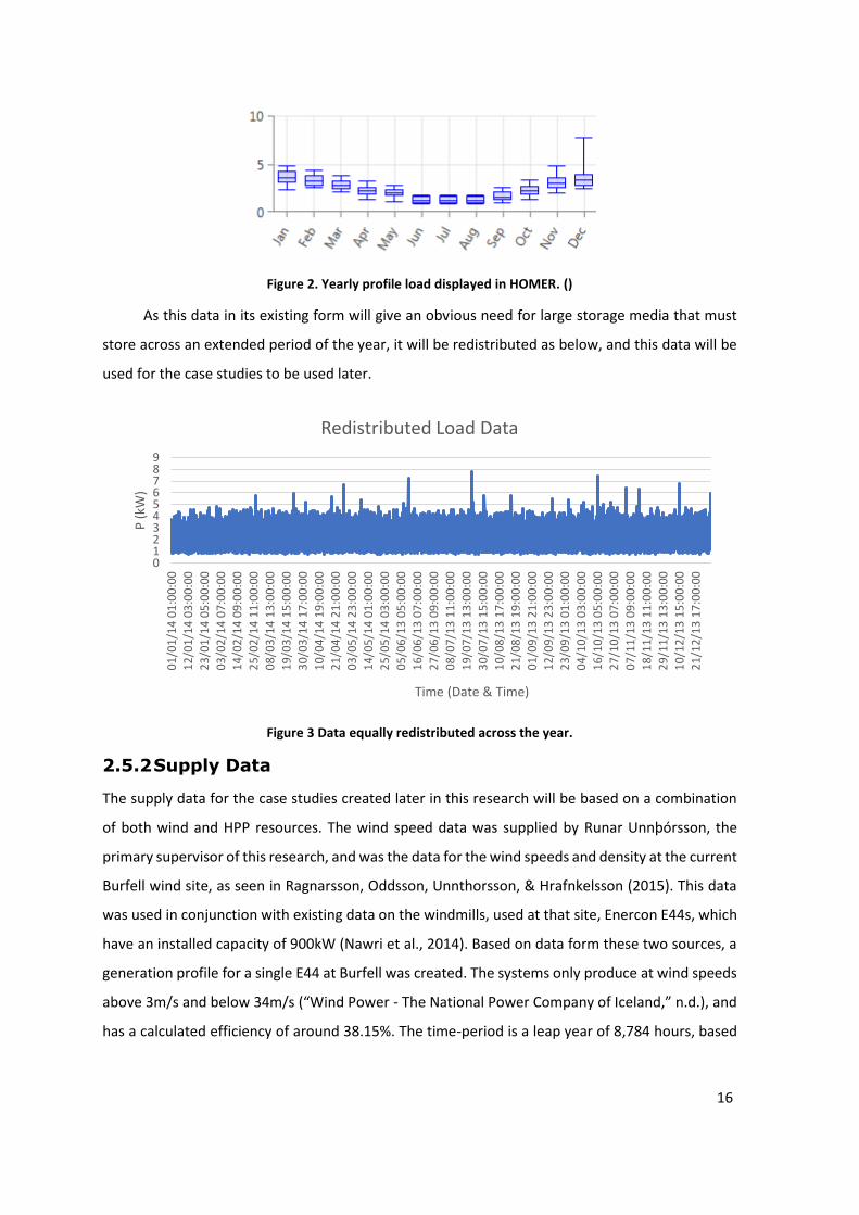
Figure 2. Yearly profile load displayed in HOMER. ()
As this data in its existing form will give an obvious need for large storage media that must
store across an extended period of the year, it will be redistributed as below, and this data will be
used for the case studies to be used later.
Figure 3 Data equally redistributed across the year.
2.5.2 Supply Data
The supply data for the case studies created later in this research will be based on a combination
of both wind and HPP resources. The wind speed data was supplied by Runar Unnþórsson, the
primary supervisor of this research, and was the data for the wind speeds and density at the current
Burfell wind site, as seen in Ragnarsson, Oddsson, Unnthorsson, & Hrafnkelsson (2015). This data
was used in conjunction with existing data on the windmills, used at that site, Enercon E44s, which
have an installed capacity of 900kW (Nawri et al., 2014). Based on data form these two sources, a
generation profile for a single E44 at Burfell was created. The systems only produce at wind speeds
above 3m/s and below 34m/s (“Wind Power - The National Power Company of Iceland,” n.d.), and
has a calculated efficiency of around 38.15%. The time-period is a leap year of 8,784 hours, based
0123456789
01
/01
/14
01
:00
:00
12
/01
/14
03
:00
:00
23
/01
/14
05
:00
:00
03
/02
/14
07
:00
:00
14
/02
/14
09
:00
:00
25
/02
/14
11
:00
:00
08
/03
/14
13
:00
:00
19
/03
/14
15
:00
:00
30
/03
/14
17
:00
:00
10
/04
/14
19
:00
:00
21
/04
/14
21
:00
:00
03
/05
/14
23
:00
:00
14
/05
/14
01
:00
:00
25
/05
/14
03
:00
:00
05
/06
/13
05
:00
:00
16
/06
/13
07
:00
:00
27
/06
/13
09
:00
:00
08
/07
/13
11
:00
:00
19
/07
/13
13
:00
:00
30
/07
/13
15
:00
:00
10
/08
/13
17
:00
:00
21
/08
/13
19
:00
:00
01
/09
/13
21
:00
:00
12
/09
/13
23
:00
:00
23
/09
/13
01
:00
:00
04
/10
/13
03
:00
:00
16
/10
/13
05
:00
:00
27
/10
/13
07
:00
:00
07
/11
/13
09
:00
:00
18
/11
/13
11
:00
:00
29
/11
/13
13
:00
:00
10
/12
/13
15
:00
:00
21
/12
/13
17
:00
:00
P (
kW)
Time (Date & Time)
Redistributed Load Data

17
on the hourly averages of the years 2004-2012, selected because the same period is available for
supplied wind data and river flows, seen below.
Figure 4. Wind power generation based on original Burfell data.
The river flowrates, in m3/s, are taken from a river in the Kirkjubæjarklaustur region, called
Geirlandsá, supplied by The Icelandic Meteorological Office (2017). The data is based on monthly
averages, as opposed to hourly averages, as seen above.
For the sake of micro hydro, the river itself somewhat oversupplies. There is an accessible
upper point of the river, that would give a 𝐻 value of around 18m (ArcGIS 10.4.1, n.d.),
(“Topographic Map; Iceland South,” 2016). Calculating from this point give the whole river a
theoretical potential of around 1.92MW, so micro hydro turbines are likely to be able to create
consistent production. To test the flow rates, a theoretical turbine was created with an efficiency
of around 77.5%, which is the mean of the efficiency range given in Chen et al. (2009), and a
generation profile was created based on the previous 2004-2012 averages for each month. The
results are shown in Figure 5.
0
0,5
1
1,5
2
2,5
3
3,5
4
4,5
5
13
27
65
39
79
13
05
16
31
19
57
22
83
26
09
29
35
32
61
35
87
39
13
42
39
45
65
48
91
52
17
55
43
58
69
61
95
65
21
68
47
71
73
74
99
78
25
81
51
84
77
Po
wer
(kW
))
Time (hours)
Wind Generation (E44)

18
Figure 5. Hydro generation at Geirlandsá. Source: (The Icelandic Meteorological Office, 2017).
These generation profiles are, as can be plainly extracted, very large in relation to the load
data. As seen in Figures 2 and 3, the peak of the load is 7.79kW, so these generation rates are
somewhat over supplied. To combat this, the case study data needs to be decreased to fit a more
reasonable generation profile. First, the flow rate averages from the river are taken and reduced by
a factor of 100, to make a range of flowrates from ~0.069m3/s (60l/s) to 0.145m3/s (145l/s). This
was then fed into the same theoretical turbine. This gives 77.5% as the efficiency of the turbine,
and the reduced flowrates are put through these turbines to give a production rate shown below.
Figure 6. HPP Generation profile based on new case study data.
The visual profile is of course much the same as in Figure 5, but with much lower kW values on the
power generation axis.
0
500
1000
1500
2000
2500
1
33
9
67
7
10
15
13
53
16
91
20
29
23
67
27
05
30
43
33
81
37
19
40
57
43
95
47
33
50
71
54
09
57
47
60
85
64
23
67
61
70
99
74
37
77
75
81
13
84
51
Po
wer
(kW
)
Time (Hours)
Theoretical HPP at Geirlandsá
0
5
10
15
20
25
1
32
7
65
39
79
13
05
16
31
19
57
22
83
26
09
29
35
32
61
35
87
39
13
42
39
45
65
48
91
52
17
55
43
58
69
61
95
65
21
68
47
71
73
74
99
78
25
81
51
84
77
Po
wer
(kW
)
Time (hours)
Downsized HPP production

19
For the wind generation profile, as the process of creating the generation profile is somewhat
more complex, a simpler method of creating smaller data will be generated. As the The old wind
profile was carried out as before, and then output of this method was also reduced by a factor of
100. In this case, the proposed theoretical wind turbine is assumed to function as the E44, but
simply only have an installed capacity of 9kW. The other features of the turbine remain the same,
apart from the efficiency value. At the defence of this research the faculty representative, Sæþór
Ásgeirsson, suggested a 25% efficiency as being more realistic, and this is taken as the assumption
for this piece. The profile is shown in Figure 7.
Figure 7. Wind Generation based on case study data.
To calculate the amount available for production, a sum value of the two profiles is shown
below. The upper value is around 25kW, and the lowest production is around 9kW.
Figure 8. Combined case study data generation profile.
0
1
2
3
4
5
13
15
62
99
43
12
57
15
71
18
85
21
99
25
13
28
27
31
41
34
55
37
69
40
83
43
97
47
11
50
25
53
39
56
53
59
67
62
81
65
95
69
09
72
23
75
37
78
51
81
65
84
79
Gen
erat
ion
(kW
)
Time (hours)
Theoeretical Wind Power Production
0
5
10
15
20
25
13
27
65
3
97
9
13
05
16
31
19
57
22
83
26
09
29
35
32
61
35
87
39
13
42
39
45
65
48
91
52
17
55
43
58
69
61
95
65
21
68
47
71
73
74
99
78
25
81
51
84
77
Po
wer
(kW
)
Time (hours)
Sum Generation

20
The data leaves a surplus, after an assumed conversion for household and grid usage or around
90% (based on the HOMER archive’s converter), of around 18.73kW, across the year. This leaves an
average of around 51.31kWh in a day, and an average of 2.14kWh in each hour for use. This is, of
course, true in theory, but needs to be accounted for across the year, as at some points the
production will not meet the load, and the reservoir will be required to discharge.
Figure 9 supplies and outlines the base system that the main cases studies will use as their
base, which all the other systems will be developed from. It contains a 9kW wind turbine, a 16kW
micro-HPP turbine, and a reservoir.
Figure 9. Outline of Combined Power System.

21

22
3 Storage Systems for Microgrids: An
Assessment of literature
3.1 Existing Storage Technologies
First the current state of the art in the form of ESS must be established. This includes a description
of the physical processes of each, an analysis of their strengths and weaknesses for micro
application. After this, the practical application of the current ESS state of the art will be measured
for small scale use. A key focus of the comparison will be the features that make a system usable
or unusable on a micro scale. The final analysis will focus on a series of barriers to small scale use,
identified from an extensive literature review of previous research on storage.
3.1.1 Description of Storage Processes
Taking a lead from Evans, Strezov, & Evans (2012) and Suberu, Mustafa, & Bashir (2014), the existing
storage technologies will be assessed and placed into the following Categories:
• Mechanical Storage (Compressed Air Storage, reservoirs, and flywheel storage)
• Electrical Storage (Capacitors/Supercapacitors/Ultracapacitors & Superconducting
Magnetic Energy Storage)
• Thermal Energy Storage (Low and high temperature technologies).
• Chemical Storage (All batteries, fuel cells, and thermochemical solar storage).
3.1.2 Mechanical Storage Technologies
Compressed Air Energy Storage
Compressed Air Energy Storage (hereafter CAES) is a system of storing electricity through the
pressurised air stored either underground in caverns, or in above ground tanks (Evans, Strezov, &
Evans, 2012). The air is then passed through a traditional gas turbine for generation purposes. The
turbine exhaust is also used to maintain the air’s heat within the cabin in many systems, (Ibrahim,
Ilinca, & Perron, 2008), (Díaz-González, Sumper, Gomis-Bellmunt, & Villafáfila-Robles, 2012).
The process of CAES has been used previously in combination with traditional gas plants to
store energy for increased efficiency and savings. However, so-called AA-CAES (Advanced Adiabatic
Compressed Air Storage), which uses solely compressed air, is also a possibility (Evans, Strezov, &
Evans, 2012). Ibrahim, Ilinca, & Perron (2008), relates that the standard gas power plants use up
two thirds of available power to compress combustion air anyway. So, the process of storing this

23
compressed air, and using it to generate in peak times in a conventional turbine, produces three
times the power for the same natural gas fuel consumption (Ibrahim, Ilinca, & Perron, 2008). This
allows for storage at off peak times, and sale and dispatching of energy at high demand times
(Rahman, Rehman, & Abdul-Majeed, 2012).
A typical CAES system is made up of the following elements (Evans, Strezov, & Evans, 2012):
• A motor or generator.
• An air compressor of two or more stages.
• A cavity or container for storage of the air.
• A turbine train.
• Controls and Auxiliaries.
Pumped Storage & Conventional Hydroelectric
Though this research will focus on the use of Micro HPPs with no pumped aspect, a large majority
of existing research literature focuses on the use of PSH. As a result, a lot of the data and
characteristics used here is based on PSH.
PSH revolves around using low demand period energy to pump water to a higher reservoir,
this water is then released through a hydroelectric turbine during high demand periods (Evans,
Strezov, & Evans, 2012). The conventional form, consisting of two reservoirs at different elevations,
with a turbine and pump between the two, is the most common (Rahman, Rehman, & Abdul-
Majeed, 2012), (Ibrahim, Ilinca, & Perron, 2008). A less conventional system is also possible, using
a mineshaft or other underground cavity as an upper reservoir and then released into the seas via
a turbine at times of high electricity demand (Evans, Strezov, & Evans, 2012), (Rahman, Rehman, &
Abdul-Majeed, 2012), (Chen et al., 2009). It is also possible to use conventional dams, without
pumps, to store electricity for demand peaks (Rahman, Rehman, & Abdul-Majeed, 2012).
PSH systems generally consist of the following (Ibrahim, Ilinca, & Perron, 2008), (Rahman,
Rehman, & Abdul-Majeed, 2012):
• Two reservoirs (conventional or otherwise).
• A pump.
• A water turbine and motor for generation.
• An external power source for the pump (where applicable in PSH).
Flywheel storage
Flywheel storage is a storage system that makes use of mechanical and kinetic energy to store and
dispatch energy. Motors are used to charge the flywheel by spinning it, the same motor is then
reversed to be used as a generator (Díaz-González, Sumper, Gomis-Bellmunt, & Villafáfila-Robles,

24
2012), (Evans, Strezov, & Evans, 2012). The result is the kinetic energy used to speed the motor is
then discharged by the slowing of the flywheel. This causes the generator to spin, creating the
required electricity at peak times (Díaz-González, Sumper, Gomis-Bellmunt, & Villafáfila-Robles,
2012), (Evans, Strezov, & Evans, 2012). To prevent drag from restricting the device’s efficiency, the
flywheel and component parts are housed in a vacuum (Díaz-González, Sumper, Gomis-Bellmunt,
& Villafáfila-Robles, 2012), (Ibrahim, Ilinca, & Perron, 2008). The electricity is generated and stored
in Direct Current (DC), (Rahman, Rehman, & Abdul-Majeed, 2012), (Díaz-González, Sumper, Gomis-
Bellmunt, & Villafáfila-Robles, 2012). They are more suited to short term uses in electricity storage,
due to self-discharge, as opposed to the longer-term applications of PSH and CAES (Baker, 2008).
A typical flywheel storage system is made up of the following (Díaz-González, Sumper, Gomis-
Bellmunt, & Villafáfila-Robles, 2012), (Ibrahim, Ilinca, & Perron, 2008):
• A pair of magnetic bearings (decreases friction).
• A Motor/generator for charging and generation.
• A composite rim for the main wheel body.
• A converter (DC energy is required for the motor, and is output by the generator).
• A vacuum for housing.
3.1.3 Electrical Storage Technologies
Capacitors and Supercapacitors
Capacitors are roughly speaking an outdated system of storage that have been eclipsed by
supercapacitors (Evans, Strezov, & Evans, 2012). Basic capacitors work by storing electricity
between two electrodes (metal plates) separated by a dielectric (insulator) (Evans, Strezov, &
Evans, 2012). Their limited storage capacity is the major reasoning for their obsolescence.
Supercapacitors, also called electric double layer capacitors and ultracapacitors, function
with a greater capacity than the conventional capacitor (Rahman, Rehman, & Abdul-Majeed,
2012). Like capacitors, they make use of two electrodes, but the dielectric insulator is replaced
with an electrolyte and the electrodes are made up of porous membranes (Díaz-González,
Sumper, Gomis-Bellmunt, & Villafáfila-Robles, 2012). They are also characterised by a smaller
separation distance between the two electrodes (Evans, Strezov, & Evans, 2012). The porous
nature of the membrane increases the surface area of the electrode, storing greater amount of
electricity (Chen et al., 2009).
An average supercapacitor set up consists of the following (Díaz-González, Sumper, Gomis-
Bellmunt, & Villafáfila-Robles, 2012):

25
• Two electrodes (usually made of a porous material).
• An electrolyte (between the electrodes, made of several possible materials).
• A converter (for electricity input and output on charge and discharge).
Superconducting Magnetic Electrical Storage
Superconducting Magnetic Electrical Storage (hereafter SMES) is a magnetic system for the storage
of electrical energy. A superconducting coil has DC current electricity run through it, creating a
magnetic field which is the electricity storage medium (Díaz-González, Sumper, Gomis-Bellmunt, &
Villafáfila-Robles, 2012). The coils operate at low temperatures, ranging from 5 to 70 Kelvin, which
is a range of -238 to -203 Celsius (Díaz-González, Sumper, Gomis-Bellmunt, & Villafáfila-Robles,
2012). The superconductivity of the coil is dependent on these low temperatures, which are
maintained through the application of either liquid nitrogen (High Temperature SMES), or liquid
helium (low temperature SMES) (Chen et al., 2009), (Hall & Bain, 2008).
A typical SMES system is made up of the following (Chen et al., 2009), (Rahman, Rehman, &
Abdul-Majeed, 2012):
• A Superconducting coil.
• A refrigeration system or medium (liquid nitrogen or liquid helium).
• An AC/DC converter.
3.1.4 Thermal Storage Technologies
Low Temperature Thermal Storage
Aquifer Systems:
Aquifer Low Temperature Energy Storage is a specifically thermal energy storage that serves
specifically for space heating rather than for electricity, making it unsuitable for this research’s
comparison (Evans, Strezov, & Evans, 2012). The system is based around the pumping of heated
water from underground aquifers to heat above ground space (Bloemendal, Olsthoorn, & Boons,
2014).
Cryogenic Systems
Unlike aquifer systems, cryogenic systems can be used to store and generate electricity (Evans,
Strezov, & Evans, 2012). The system also uses off-peak renewable generation systems to store
electricity for peak demand times (Evans, Strezov, & Evans, 2012). This system revolves around air
liquefaction to make cryogenic fluid for use in a cryogenic heat engine to generate electricity (Evans,
Strezov, & Evans, 2012).
A cryogenic ESS generally consists of (Evans, Strezov, & Evans, 2012) (Abdo et al., 2015):

26
• A cryogenic plant for fluid generation.
• A cryogenic tank for storage.
• A cryogenic heat engine.
High Temperature Thermal Storage
Sensible Heat Storage
Sensible Heat storage systems make use of multiple possible types of heat storage media to store
heat for energy generation uses (Evans, Strezov, & Evans, 2012). Possible media include graphite,
concrete, molten salt, hot rocks, and steam/hot water accumulators (Evans, Strezov, & Evans,
2012). The stored heat is then recovered by the creation of water vapour to turn a generator (Evans,
Strezov, & Evans, 2012). Sensible Heat is defined as using storage materials that do not undergo
any kind of phase change (Gil et al., 2010). Sensible heat systems are also used for heating systems,
such systems have been dispatched in the UK (Baker, 2008). The heat storage systems include a
variety of storage materials, including solids and liquids (Gil et al., 2010).
Sensible heat energy storage systems generally consist of (Evans, Strezov, & Evans, 2012), (Gil
et al., 2010):
• A Storage Medium (any of those listed above).
• A Water vapour powered turbo-alternator.
• An electrical source to generate stored heat.
Latent Heat Storage
Latent heat systems are differentiated from sensible heat systems by the fact that they use heat
derived from phase change materials. (Evans, Strezov, & Evans, 2012). Inorganic salts, metals and
paraffin are used for the storage media, and their transition between states heats a liquid heat
transfer fluid to capture the heat for electrical generation (Evans, Strezov, & Evans, 2012). When
charging or storing the energy, a solid is either liquefied or crystallised before this process is
reversed for the generation (Evans, Strezov, & Evans, 2012). The phase change materials (hereafter
PCMs) need to be non-corrosive, non-toxic, and have a high melting temperature, with high thermal
conductivity to be effective (Qureshi, Nair, & Farid, 2011). This system is often used in solar
applications, as there is no need to convert the direct heat from the sun into electricity for storage,
increasing its efficiency (Evans, Strezov, & Evans, 2012), (Qureshi, Nair, & Farid, 2011).
Information on a specific and traditional Latent Heat generation model is not available, but
this is likely due to the multiple PCMS available, requiring a range of operating heats and costs (Gil
et al., 2010), leading to a multitude of possible systems.

27
3.1.5 Chemical Storage Technologies
Chemical Energy Storage; Batteries
Battery technology is the most varied storage system. This research will summarise the following
battery types; Lead Acid (hereafter Pb-Acid), Sodium Sulphur (hereafter Na-S), Flow Batteries,
Nickel Batteries (Iron [hereafter Ni-Fe], Cadmium [hereafter Ni-Cd], Hydrogen [hereafter Ni-H2],
Metal Hydride [hereafter Ni-MH], Nickel-Zinc [hereafter Ni-Zn], and Sodium Nickel-Chloride
[hereafter ZEBRA batteries]), Lithium ion (hereafter Li-ion, both cobalt and phosphate based), and
Metal Air batteries.
Pb-Acid Batteries
These batteries store electricity through, as the name suggests, a combination of a sulphuric acid
electrolyte and two lead electrodes; a lead acid cathode and a spongy lead anode (Evans, Strezov,
& Evans, 2012). The lead serves as the collector of the stored current (Evans, Strezov, & Evans,
2012). There are, as with Latent Heat storage systems, several formats; A flooded Pb-Acid battery,
filled with a water-sulphuric acid solution, a sealed Pb-Acid battery, which substitutes the water for
a gelled electrolyte, and the valve regulated Pb-Acid battery (Chen et al., 2009). However, it’s
possible to summarise the common features of a Pb-Acid battery as follows (Rahman, Rehman, &
Abdul-Majeed, 2012), (Chen et al., 2009);
• A lead-acid cathode.
• A spongy lead anode.
• A sulphuric acid based electrolyte.
• A separator to separate the cathode and anode charge.
Na-S Batteries
As the name suggests, the energy storage in this battery is the result of a chemical reaction between
Sodium and Sulphur. Kept in a molten state, the Sodium acts as the cathode, the Sulphur as the
anode (Chen et al., 2009). These molten electrodes are separated by a ceramic electrolyte, which
allows only the positive sodium ions to flow through. This forms sodium polysulphide, acting as the
storage medium. During discharge, the positive sodium ions flow back through it, along with
electrons to generate (Chen et al., 2009). A typical Na-S Battery would consist of the following (Chen
et al., 2009):
• Molten sulphur for the anode.
• Molten sodium for the cathode.
• A ceramic electrolyte.

28
The systems must operate at around 300-350C, which requires energy for the heating itself
(Rahman, Rehman, & Abdul-Majeed, 2012). This can be achieved through using the battery’s own
generation system (Rahman, Rehman, & Abdul-Majeed, 2012), or an external energy source (Baker,
2008).
Flow Batteries
These batteries are divided into two categories; redox and hybrid batteries (Evans, Strezov, & Evans,
2012). Redox flow batteries use two separate electrolytes, one positive and one negative, which
flow through a cell containing a carbon felt, serving as an inert electrode (Rahman, Rehman, &
Abdul-Majeed, 2012). The electrolytes serve to both store and discharge the electricity, as they
both collect their charge in the cell and discharge in by being passed through it, converting chemical
energy to electricity (Chen et al., 2009), (Rahman, Rehman, & Abdul-Majeed, 2012). A typical Redox
battery contains the following (Chen et al., 2009), (Rahman, Rehman, & Abdul-Majeed, 2012);
• Two Electrolyte tanks.
• A positive and negative electrolyte.
• Two pumps, to move the electrolyte through the cell.
• Carbon felt, acting as an inert electrode.
Hybrid flow batteries operate using a similar process, but using different electrolytes, and
making use of different chemical flows. There are two main types of hybrid flow systems; Zinc-
Bromine batteries and Sodium-Sulphur Batteries (or polysulphide batteries) (Díaz-González,
Sumper, Gomis-Bellmunt, & Villafáfila-Robles, 2012). In Zinc-Bromine systems, the Bromide serves
as the anode, the Zinc as the cathode (Díaz-González, Sumper, Gomis-Bellmunt, & Villafáfila-Robles,
2012). For Sodium-sulphur systems, Sodium-bromide and Sodium-sulphide are used as the
electrolytes. The Sodium-bromide serves as the positive once again, the Sodium-sulphide as the
negative (Díaz-González, Sumper, Gomis-Bellmunt, & Villafáfila-Robles, 2012). In all these, systems,
as with redox systems, the chemical changes in these substances is used to generate electricity
from chemical energy. Their structure is not dissimilar from redox flow batteries, with separate
electrolytes in tanks flowing through production cells (Díaz-González, Sumper, Gomis-Bellmunt, &
Villafáfila-Robles, 2012), (Evans, Strezov, & Evans, 2012).
Nickel Battery Systems
Ni-Fe Batteries
In these systems, the Nickel comes in the form of nickel oxyhydroxide, which serves as the anode
in the battery, while iron serves as the cathode (Shukla, Venugopalan, & Hariprakash, 2001). An
alkaline solution serves as the electrolyte in this battery system (Shukla, Venugopalan, &

29
Hariprakash, 2001). Cell reactions are used to generate electricity and to store it for later, as with
most chemical storage systems (Shukla, Venugopalan, & Hariprakash, 2001). Cells contain the
electrodes of different charges arranged alongside one another and separated by a porous
membrane (Shukla, Venugopalan, & Hariprakash, 2001). So, the standard components of a Ni-Fe
Battery can be summarised as (Shukla, Venugopalan, & Hariprakash, 2001);
• A Nickel Oxyhydroxide electrode.
• An Iron electrode.
• An alkaline solution, serving as a medium.
Ni-Cd Batteries
Ni-Cd batteries make use of a Nickel anode, and a negative electrode made of cadmium. At the
cathode, nickels hydroxide and nickelic hydroxide are transferred between during charge and
discharge (Shukla, Venugopalan, & Hariprakash, 2001). Discharge is made from the discharge of
cadmium hydroxide at the anode. For charging purposes, it is converted into metallic cadmium
(Shukla, Venugopalan, & Hariprakash, 2001). The systems all make use of an electrolyte (Shukla,
Venugopalan, & Hariprakash, 2001). A typical Ni-Cd system contains the following (Shukla,
Venugopalan, & Hariprakash, 2001);
• A Nickel anode.
• A cadmium cathode.
• A potassium hydroxide electrolyte.
• Separators between each pair of electrodes (often nylon).
Ni-Cd suffer from a unique weakness in the form of the memory effect, whereby they must
be fully discharged before recharging to be fully efficient (Shukla, Venugopalan, & Hariprakash,
2001).
Ni-H2 Batteries
Ni-H2 batteries don’t function too dissimilarly from Ni-Cd batteries, replacing the cadmium element
with a hydrogen gas electrode, and using a range of materials as separators (Shukla, Venugopalan,
& Hariprakash, 2001). Available information on the battery type (Shukla, Venugopalan, &
Hariprakash, 2001) suggests a variety of designs are available, so a typical configuration is less
positively identified. However, it certainly includes the following (Shukla, Venugopalan, &
Hariprakash, 2001);
• A nickel anode.
• A hydrogen gas cathode.
• A separator.

30
• A potassium hydroxide electrolyte solution.
Ni-MH Batteries
Ni-MH batteries are also similar to Ni-Cd systems; these batteries also use a nickel oxyhydroxide
anode, but the cathode is this time made up of hydrogen storage alloys (Evans, Strezov, & Evans,
2012), (Shukla, Venugopalan, & Hariprakash, 2001). As always, there is an electrolyte as well as a
separator making up the space between electrodes (Shukla, Venugopalan, & Hariprakash, 2001).
The energy itself is stored in the hydrogen alloys in the form of Hydrogen itself (Shukla,
Venugopalan, & Hariprakash, 2001). So, a typical Ni-MH battery is made up of the following (Shukla,
Venugopalan, & Hariprakash, 2001);
• A Nickel anode.
• A Hydrogen storage alloy cathode.
• A separator (multiple possible materials).
• A potassium hydroxide electrolyte.
They have a higher charge efficiency than Ni-Cd batteries, and operate at a range of
temperatures from -20C to 45C (Shukla, Venugopalan, & Hariprakash, 2001). However, their
discharge rate is noted to be higher than with Ni-Cd (Shukla, Venugopalan, & Hariprakash, 2001).
Ni-Zn Batteries
A combination of zinc and nickel electrodes are also similar in function to the previously discussed
nickel batteries. A similar electrolyte of potassium hydroxide, at a 20-35% solution, is also used in
the function of these batteries (Shukla, Venugopalan, & Hariprakash, 2001). The nickel once again
serves as the cathode here, with zinc making up the anode (Shukla, Venugopalan, & Hariprakash,
2001). This means a Ni-Zn system can be summarised as follows (Shukla, Venugopalan, &
Hariprakash, 2001):
• A zinc anode.
• A nickel cathode.
• A potassium hydroxide electrolyte.
• A separator (several possible materials).
ZEBRA Batteries
The ZEBRA battery, so named when it was invented in South Africa (ZEBRA is an acronym of Zeolite
applied to Battery Research Africa), is perhaps as related to a sodium battery as a nickel one (Hall
& Bain, 2008). Functioning using a sodium electrode in combination with a ceramic separator
(Shukla, Venugopalan, & Hariprakash, 2001). They operate at a high temperature (300C) and need

31
to be kept attached to a separate generating source to be ready to operate when called on (Shukla,
Venugopalan, & Hariprakash, 2001). A rough overview of the typical system would include (Shukla,
Venugopalan, & Hariprakash, 2001):
• A sodium electrode.
• A nickel electrode.
• A ceramic separator.
• An external energy sources.
Their high 300C operating temperature is shared by Na-S systems, and requires external
energy to be maintained (Hall & Bain, 2008), (Shukla, Venugopalan, & Hariprakash, 2001). If fully
discharged and then left before being recharged, echoing the Ni-Cd memory effect, reaching the
desired operation temperature can take 2 to 4 days (Shukla, Venugopalan, & Hariprakash, 2001).
Li-Ion systems
Li-Ion batteries can be either cobalt or phosphate based (Evans, Strezov, & Evans, 2012). Both these
systems make use of a lithium (or lithiated metal) cathode and a carbon (or graphite) anode, with
a dissolved lithium salt and organic carbonate electrolyte (Divya & Østergaard, 2009) (Díaz-
González, Sumper, Gomis-Bellmunt, & Villafáfila-Robles, 2012). Lithium atoms are created in the
charging process, and this chemical reaction is reversed for the discharge process (Divya &
Østergaard, 2009). From a technical standpoint, a phosphate based Li-Ion has higher efficiency in
storage and conversion (Evans, Strezov, & Evans, 2012). So, a typical system would be considered
to include the following (Divya & Østergaard, 2009);
• A lithium anode.
• A carbon or graphite cathode.
• An electrolyte of lithium salt and organic carbonate.
Metal Air Batteries
The metals most commonly used in this type of battery are zinc and aluminium, which serve as the
cathode in these battery systems (Chen et al., 2009). The anode is often made up of a porous carbon
structure (Chen et al., 2009). The common electrolyte is a potassium hydroxide solution. Sometimes
this is applied to a solid polymer membrane (Divya & Østergaard, 2009). A common system would
contain the following (Chen et al., 2009), (Divya & Østergaard, 2009):
• A zinc or aluminium cathode.
• A porous “air” anode (often carbon).
• A potassium hydroxide electrolyte.
• A solid electrolyte coated in potassium hydroxide (occasionally).

32
These systems make for compact battery systems, and unlike Pb-acid or Ni-Cd batteries,
there is little environmental impact (Chen et al., 2009).
Electrochemical Energy Storage; Fuel Cells
Fuel cells most frequently make use hydrogen for the production and storage of energy. Commonly,
an electricity source generates Hydrogen from water through use of an electrolyser, which is then
stored in a variety of ways (Díaz-González, Sumper, Gomis-Bellmunt, & Villafáfila-Robles, 2012). The
fuel in the cell then acts as the anode in the device, and reacts with oxidant cathode, the reaction
of which happens in the presence of an electrolyte to generate electricity (Evans, Strezov, & Evans,
2012), (Chen et al., 2009). It is different from Batteries in this way, as the fuel is used up in this
reaction, and must be replenished (Chen et al., 2009). Though a few fuels are possible, Hydrogen
fuel cells are one of the most covered fuels in literature, so the fuel cell system is summarised
roughly as follows (Chen et al., 2009), (Díaz-González, Sumper, Gomis-Bellmunt, & Villafáfila-
Robles, 2012), (Evans, Strezov, & Evans, 2012);
• An external electricity supply.
• An electrolyser (for hydrogen creation).
• A fuel (in this research summary, Hydrogen).
• An oxidant to react with the fuel (e.g. oxygen in a hydrogen cell).
• An electrolyte for syphoning electricity for use.
Depending on the method of storage, Hydrogen fuel cells may have no self-discharge
whatsoever (Díaz-González, Sumper, Gomis-Bellmunt, & Villafáfila-Robles, 2012). Other fuel cell
systems include direct-methanol fuel cells, molten carbonate fuel cells, and solid oxide fuel cells
(Chen et al., 2009).
Thermochemical Energy Storage; Solar Storage Systems
Solar storage is a system of storing solar heat for energy use later. Evans, Strezov, & Evans (2012)
categorise the four solar systems into solar hydrogen, solar metal, solar methane and solar
ammonia. Anderson & Leach (2004) cover the use of concentrated solar heat to create a synthesis
gas of methane and carbon dioxide, which can be stored and desynthesised to use that energy later.
Solar hydrogen is a diverse system, in which 5 possible processes are used to create hydrogen from
water, and one of these processes makes use of conventional fossil fuels (Chen et al., 2009). In all
cases, the focus is on high temperature solar heat being used to create storable gases (Chen et al.,
2009).
Solar metals involve the storing of solar energy in metals, commonly Zinc. This is then either
used to create elevated temperatures or to generate electricity in a fuel cell (Chen et al., 2009). The
latter ammonia based and methane based systems use solar heat to catalyse an endothermic

33
chemical reaction for the long-term storage, only for this to be reversed in an exothermic reaction
for electricity generation later (Chen et al., 2009). As noted by Evans, Strezov, & Evans (2012) Solar
storage systems are not in a high level of maturity, so a typical system cannot be assembled.
3.2 Storage Comparison for Small-Scale or
Micro-Grid Applications
As this research focuses on which of the existing technologies are best applied to a small-scale
electricity production and storage system, it is necessary to establish comparison criteria. As stated,
the final case study analysis of this research will focus on a Micro HPPs, which is less than 1MW, so
the need to understand storage equivalent technologies will first be established. Through reading
existing research, the following comparison areas will be taken for comparative analysis:
• Scalability: technologies that become less efficient or too costly at small scales are, of
course, unsuitable.
• Density: both energy and power density (kW provided in relation to size, either weight (kg)
or volume (l)) are key factors as they contribute to the overall system sizing.
• Efficiency: the ability to store and discharge energy efficiently is a desirable feature of each
technology. Those with high efficiencies will be balanced against their other weaknesses
and shortcomings.
• Scale and Time of Storage: For small scales, it is suitable to store a relative high
(proportionally speaking) amount of energy for both long and short terms. This helps with
the ability to meet energy demands on both yearly peak and daily requirement terms.
• Proven Status: If a storage technology is not commercially available, or only exists in an
experimental capacity, it will be eliminated.
• Costs: Specifically, the Net Present Values of Costs (NPVs or NPCs) or LCOEs have been
covered in previous research, and this information will be used to provide an understanding
of the real differences in costs between these different technologies.
• Life span: with a great variance in overall life spans noted, knowing the effects these will
have on other areas of comparison is of key importance.
• Restrictions of applicability: CAES and PSH are noted to specific geographical applications.
Other technologies (such as Pb-Acid are noted for having higher environmental impacts.
Some may even have hidden costs, such as the price of replacement, or decommissioning.
Finally, some are simply unsuitable for housing use grade electricity. An overview of these
concerns will be presented.

34
3.2.1 Scalability
PSH installations are generally of a considerable size, with large installations ranging from 200MW
– 2,710MW existing worldwide (Evans, Strezov, & Evans, 2012). This does not exclude them from
use at a micro level, but questions the applicability of data based on them to the small-scale power
dam considered by this research.
PSH is considered by the works of Chen et al. (2009), Ibrahim, Ilinca, & Perron (2008), and
Rahman, Rehman, & Abdul-Majeed (2012) to be specifically considered an “energy management”
storage technology. These are technologies focused on managing the energy supply by storing
electricity for use in times when generation falls short (Chen et al., 2009), (Ibrahim, Ilinca, & Perron,
2008), (Rahman, Rehman, & Abdul-Majeed, 2012). This suggests they can be used for small grids,
as this type of storage is described as providing “grid independence” (Rahman, Rehman, & Abdul-
Majeed, 2012). The issue of scalability for PSH is best explained by another of their defining
characteristics, their energy density. It is so low with PSH, which may necessitate larger installations
(Luo, Wang, Dooner, & Clarke, 2015).
Luo, Wang, Dooner, & Clarke (2015) also point to a low scalability for both underground
CAES and aboveground CAEs storage. They both have a fairly high cost/kW, but, most importantly
are also similarly low in energy and power density to PSH systems (Evans, Strezov, & Evans, 2012),
(Luo, Wang, Dooner, & Clarke, 2015). This puts both on a comparatively low downward scalability.
Systems which are noted to have a good downwards scalability are flywheels and SMES
systems (Luo, Wang, Dooner, & Clarke, 2015). This will be expanded on later, as it is a result of their
capital costs being very favourable in terms of power, if not energy, density (Luo, Wang, Dooner, &
Clarke, 2015). This is also noted for superconductor technologies which have also penetrated small
scale applications like automobiles and portable electronics, as stated earlier (Hall & Bain, 2008).
Battery systems vary in their comparative scalability to microgrid usage. For instance, there
is a noted use of very small-scale Ni-MH in the realm of portable electronics (Hall & Bain, 2008). Pb-
Acid systems, partly due to their maturity (as will be discussed later), are also noted for their ability
to be used at a range of sizes and applications (Evans, Strezov, & Evans, 2012). Pb-acid have also
been considered for similar scale generation studies beforehand (Kalantar & Mousavi G., 2010). Li-
Ion batteries are generally known for their scalability to be used in very small-scale technologies,
such as electronics, (Luo, Wang, Dooner, & Clarke, 2015), however it is noted that in fact the
scalability towards large scale storage, like storing domestic electricity, is yet to be tried effectively
(Pickard, Shen, & Hansing, 2009). It is also noteworthy that many small-scale studies have suggested
batteries of unspecified types to test similar scenarios to the ones studied in this paper (Alkababjie
& Hamdon, 2012), (Diaf, Belhamel, Haddadi, & Louche, 2008), (Li, Zhu, Cao, Sui, & Hu, 2009). While

35
Pb-Acid, Na-S and Ni-Cd batteries are noted to have high maximum capacities, at ~10MW, and
~27MW respectively, other battery types are generally >1.5MW in capacity (Suberu, Mustafa, &
Bashir, 2014). The data for this area based on flow batteries is currently unavailable so cannot be
accounted for.
Hydrogen fuel cells on a small-scale are already commercially available, and like battery
technologies, have been considered on comparative scales before. For example, fuel cells of
~2.4kW capacity are looked at in combination with 13-25kW capacity electrolysers and ~2.2MWh
hydrogen tanks in the works of Li, Zhu, Cao, Sui, & Hu (2009). This comparable to the 2kW capacity
fuel cells, studied in the works of Maclay, Brouwer, & Samuelsen (2006). The highest commercially
available unit of fuel cell is 15MW (Suberu, Mustafa, & Bashir, 2014). Generally, fuel cells can be
considered to have a reasonable scalability.
Regarding thermal systems, cryogenic storage systems have the least available data to be
considered. However, as high energy is required for their fluid production (Evans, Strezov, & Evans,
2012), their separation from grids for independence purposes is questionable. This does not
indicate that functioning thermal systems at a small scale are non-existent, of course. In fact, high
temperature latent systems are listed as having a capacity from 0 - 60MW, indicating a potential
for small applications (Evans, Strezov, & Evans, 2012). As noted, it is unlikely to use solar fuel
systems from Photovoltaic (PV) scale systems, as they are usually based on concentrated solar
power systems (Chen et al., 2009).
3.2.2 Energy Density
This area of energy storage is a major influence on the scalability of all energy sources, but is also
important in its own right. Power density will not be covered in as much detail, as the focus here is
on the ability of devices to hold energy for later uses. As stated energy density is the kWh/kg, or
the kWh/l storage rate of a technology. They are summarised in Table 2 below.
Table 2 Summary of Density Values. Sources: (Chen et al., 2009), (Evans, Strezov, & Evans, 2012), (Luo,
Wang, Dooner, & Clarke, 2015), (Pickard, Shen, & Hansing, 2009), (Shukla, Venugopalan, & Hariprakash,
2001)
PSH 05.-1.5Wh/l
CAES 30-60Wh/kg
Overground CAES 140Wh/kg
Flywheels 5-100Wh/kg
Supercapacitors 2-15Wh/kg (300-500W/kg)

36
SMES 0.5-5Wh/kg
Cryogenic Thermal Storage 150-250Wh/kg
High Temperature Energy Storage 80-200Wh/kg
Fuel Cells 800-10,000Wh/kg
Li-Ion 75-200Wh/kg
Na-S 150-240Wh/kg
Ni-Cd 50-75Wh/kg
Ni-MH Unavailable
Ni-H2 53-60Wh/kg
Other Nickel Unavailable
Pb-Acid 25-50Wh/kg
Zinc Bromide Flow Batteries 15-30Wh/kg
Redox Flow Batteries 10-30Wh/kg
ZEBRA 100-120Wh/kg
Metal-Air 150-300Wh/kg
Solar Storage 800-100,000Wh/kg
3.2.3 Efficiency
For the sake of looking at micro-grids, to ensure an effective system with little waste is naturally a
key concern. As there may not be much energy generated, the ideal system will waste as little of
this as possible. This will enable the system to adequately match storage and dispatching to
shortages of generation.
PSH installations are known for a high cycle and discharge efficiency. Their cycle efficiencies
are listed at around 70-85% (Chen et al., 2009), (Evans, Strezov, & Evans, 2012), (Pickard, Shen, &
Hansing, 2009), making a large amount of the energy stored ultimately reclaimable. It is noteworthy
that there are also some sources that list their upper efficiency at as high as 87% (Luo, Wang,
Dooner, & Clarke, 2015).
Underground CAES sits in a similar region of efficiency, if slightly lower on the upper limit,
they have a much wider variety of listed efficiencies. For example, ~70-~80% is the given range in
Chen et al. (2009). However, elsewhere the range is extended from 65%-89% (Pickard, Shen, &
Hansing, 2009), (Evans, Strezov, & Evans, 2012). Strangely, there are some lower installation values
given at 42% and 54% (Luo, Wang, Dooner, & Clarke, 2015). Above ground, CAES has a more modest

37
efficiency, at 50% (Evans, Strezov, & Evans, 2012). Generally speaking, this relies on the specific
construction of each CAES site, above or below ground, and can vary a lot in function.
Batteries of most types also fall into this rough range, starting at a general low of 60-65% (Ni-
Cd and Zinc Bromine), the upper efficiencies are generally around 85-90% (Na-S, ZEBRA, Pb-Acid,
Vanadium flow), with a lot having a 75% upper efficiency (Other flow batteries) (Chen et al., 2009),
(Evans, Strezov, & Evans, 2012), (Hall & Bain, 2008), (Luo, Wang, Dooner, & Clarke, 2015), (Rahman,
Rehman, & Abdul-Majeed, 2012). Interestingly Na-S must use their own generation to maintain
heat. Without this, Na-S batteries have an 100% efficiency of energy recovery (Baker, 2008).
Thermal system, solar fuels, fuel cells in general and metal-air battery systems sit at the lower
efficiency region. They are all lower than 60%, and the lower range of all these technologies is
around 20-30% (high temperature thermal storage, hydrogen fuel cells, and solar fuels) (Evans,
Strezov, & Evans, 2012), (Luo, Wang, Dooner, & Clarke, 2015). This is explained by the fact the
systems require conversion from AC into a storage medium, resulting in a low overall cycle storage
(Chen et al., 2009). For cryogenic systems, the process of creating cryogenic fluid is a high-energy
process (air liquefaction), which affects the storage system’s efficiency, with no actual data supplied
(Evans, Strezov, & Evans, 2012).
The highest efficiency systems flywheels, Li-ion batteries, SMES, and supercapacitors. The
systems have general efficiencies greater than 90%. SMES and supercapacitors in particularly have
95% and 98% upper efficiencies listed, with 90% as their lower efficiencies (Chen et al., 2009),
(Evans, Strezov, & Evans, 2012), (Luo, Wang, Dooner, & Clarke, 2015). Li-Ion functions as the most
efficient battery, the highest being 97% (Luo, Wang, Dooner, & Clarke, 2015), but have a general
lower efficiency range of 75-85% (Evans, Strezov, & Evans, 2012), (Luo, Wang, Dooner, & Clarke,
2015). Flywheels have an efficiency range of 90-95% (Evans, Strezov, & Evans, 2012), (Luo, Wang,
Dooner, & Clarke, 2015).
3.2.4 Storage Scale and Duration
As noted by Chen et al. (2009), the rate of self-discharge in a technology has a profound effect on
its ability to be used for longer than a certain period. A short duration does not imply a negative,
but can only be applied to scenarios. In some cases, it may be better to use a system that matches
to low points in hours or a system that to matches low points in the yearly demand.
High duration technologies are considered those which can feasibly store technology for
months at a time; PSH, CAES, fuel cells, metal air batteries, all flow battery types, solar fuels, and
high temperature energy storage systems (Chen et al., 2009), (Díaz-González, Sumper, Gomis-
Bellmunt, & Villafáfila-Robles, 2012). Projections for cryogenic systems suggest that it will be

38
suitable for long term storage at a high energy density (Evans, Strezov, & Evans, 2012), putting it
theoretically in this group.
Medium duration technologies shall be considered those that extend only to days; Pb-Acid
batteries, Ni-Cd batteries, Li-Ion batteries, SMES and low temperature thermal storage (Chen et al.,
2009). SMES are suited to storing high power over a short duration, but of a duration slightly over
a day (Hall & Bain, 2008), (Kondoh et al., 2000).
Short period technologies are feasibly only usable for 24 hours or less: Na-S batteries,
ZEBRA batteries, Flywheels, and Capacitor technologies (Chen et al., 2009).
Key factors separating these technologies are their comparative daily self-discharge rates,
for example in supercapacitors this is 100% (Luo, Wang, Dooner, & Clarke, 2015), and SMES
technologies have a more medium range of 20-40% in self-discharge terms (Evans, Strezov, & Evans,
2012). Li-Ion systems have a low discharge rate, at 1-5%, but this is noted to make them useable on
a short term, as they are best suited to specific applications (Díaz-González, Sumper, Gomis-
Bellmunt, & Villafáfila-Robles, 2012). The high duration technologies range from a negligible or not
readable loss rate (CAES and PSH) to a low rate of 0.1-1% (the high duration batteries and high
temperature thermal storage) (Luo, Wang, Dooner, & Clarke, 2015).
It is noteworthy that a lot of the short duration technologies are used for storing high
energy and dispatching them quickly; this is noted for Flywheels, Li-Ion (Díaz-González, Sumper,
Gomis-Bellmunt, & Villafáfila-Robles, 2012), SMES (Hall & Bain, 2008), and supercapacitors (Hall &
Bain, 2008), (Pickard, Shen, & Hansing, 2009). Flywheels are particularly suited to a short-term
basis, making them useful for short term high power applications (Evans, Strezov, & Evans, 2012).
They are suited to use in isolated areas, something that has already been achieved in islands in
Scotland and Wales, where they manage the quality of the electricity supply (Ibrahim, Ilinca, &
Perron, 2008).
This would place them into what Ibrahim, Ilinca, & Perron (2008) refer to as “quality” power
storage systems. These are used to ensure a similar amount of power is generally available and can
thus be maintained in a stable manner (Denholm, Ela, Kirby, & Milligan, 2010). This is a key focus
of small renewable usage, as a drop off of intermittent renewable sources at certain times is the
gap the storage seeks to meet. It is also noteworthy, however, that these systems are not alone in
this category and that Pb-Acid and Ni-Cd can be used for the same application (Denholm, Ela, Kirby,
& Milligan, 2010). Despite this, the specific aim of technologies designated “energy management”
(technologies which ensure energy generation is stored for times at which they can be used, so
production peaks can be stored for demand peak usage later (Ibrahim, Ilinca, & Perron, 2008)) is
the ideal usage for storage, and it includes Pb-Acid, Flow battery, CAES, and PSH systems (Ibrahim,

39
Ilinca, & Perron, 2008). In this way, it is important to weigh up the specific small-scale application
you are looking at, as it can depend on the specific generation peaks and troughs, which may be
daily or seasonal. PSH is especially flexible in its potential uses partly due to its fast response times
of around 3-5 minutes (Dursun & Alboyaci, 2010).
3.2.5 Technological Maturity and Proven Status
The proven status of a technology is key to the understanding of its applicability to a small-scale
application. Some of the storage technologies discussed exist only in demonstration form, without
having made it to a commercial standard at the time of writing (January 2017). Furthermore, early
stage technologies are not at the height of their potential efficiency, with further research and
development being required. When applying a technology to a small-scale status, it is likely that a
commercially available technology would be required, as it is infeasible to build a completely new
system from scratch.
The three storage technologies that could be considered proven are those of Pb-Acid, PSH
and CAES. Luo, Wang, Dooner, & Clarke (2015) denote them as proven technologies, as opposed to
developing or demonstration level technologies. Pb-Acid was perhaps the first battery technology
for the storage of electricity, as it has been used for more than a century (Baker, 2008). This is
reflected in their high market penetration, as perhaps the standard form of battery storage (Chen
et al., 2009). PSH installations make up 10% of Japan’s power plant capacity (Kondoh et al., 2000),
and 40 such plants exist in the USA (Yang & Jackson, 2011). Evans, Strezov, & Evans (2012) note
that of all the storage technologies to be studied, it is the most widely used, with Baker (2008)
noting 90 GW as the worldwide installed capacity. While underground systems are less established,
with none being built, conventional PSH is already widely used (Pickard, Shen, & Hansing, 2009).
CAES currently enjoys a proven technological status, as two power plants exist and are used in large
scale systems in Germany (where a 290MW plant operates) and Alabama, USA (where a 110 MW
plant operates) (Kondoh et al., 2000), (Mason & Archer, 2012). In both systems, it is used for peak
demand supply (Mason & Archer, 2012) However, the pure air variant of CAES, AA-CAES, is a much
more recent technology (Luo, Wang, Dooner, & Clarke, 2015).
Although not as established and proven as Pb-Acid as a technology, Na-S systems have been
developed over the last 30 years, and became commercially available in 2002, and reaching 55
installations quickly by 2003 (Baker, 2008), (Evans, Strezov, & Evans, 2012). Flow Batteries being so
varied in structure have varying levels of technology, but at this point are still considered to be
developing technologies, compared to the previously established technologies (Luo, Wang, Dooner,
& Clarke, 2015). Ni-Fe batteries are of a similar maturity to Pb-Acid, developed in the beginning of

40
the 20th century, though there is less note of their market penetration (Shukla, Venugopalan, &
Hariprakash, 2001). NI-Cd, like Ni-Fe, are very mature, entering manufacturing in the 20th (Suberu,
Mustafa, & Bashir, 2014), (Shukla, Venugopalan, & Hariprakash, 2001). They are proven system, but
also one that has declined in use due to the advantages offered by alternative nickel batteries like
Ni-MH, which have somewhat replaced Ni-Cd batteries for certain applications (Evans, Strezov, &
Evans, 2012), (Shukla, Venugopalan, & Hariprakash, 2001). Ni-MH Batteries have proven
technological uses in such as portable batteries, and electrical vehicle use (Evans, Strezov, & Evans,
2012), (Shukla, Venugopalan, & Hariprakash, 2001). Ni-Zn are considered a proven and
commercially available technology, being constructed for sale in China and the United States
already (Shukla, Venugopalan, & Hariprakash, 2001). Lastly for nickel systems, ZEBRA batteries are
considered to be developed if not fully mature, by Chen et al. (2009), which the research defines
are being a result of being commercially available, but lacking real market penetration. Li-Ion are a
mature and widely used battery source, being used in small scale applications, like mobile phones
(Díaz-González, Sumper, Gomis-Bellmunt, & Villafáfila-Robles, 2012). Díaz-González, Sumper,
Gomis-Bellmunt, & Villafáfila-Robles (2012) even note the annual battery production rates are
around 2 billion cells. Phosphate based Li-Ion systems are a less proven and more recent technology
(Evans, Strezov, & Evans, 2012).
Similarly developed but not fully proven and mature technologies include flywheels, all of
the electrical storage systems, (SMES, and Supercapacitors), and high temperature thermal storage
systems (Chen et al., 2009). Of the mechanical storage systems discussed, flywheels are the least
proven in status, as well as the least mature and used. Though the devices enjoy a life span in excess
of 20 years, commercial uses were yet to be applied as of 2008 (Hall & Bain, 2008). Suzuki, Koyanagi,
Kobayashi, & Shimada (2005) have completed works considering it as a potential technology to
prevent supply interruptions, which establishes existing produced technologies. Larger flywheels
do exist, as seen in the Smart Energy Matrix 20MW Frequency Regulation Plant, located in
Massachusetts (Pickard, Shen, & Hansing, 2009). SMES’s maturity and usability of the system is
established, with six plants in operation in the United States, and some commercially available
products in existence, but the market penetration is low (Hall & Bain, 2008), (Pickard, Shen, &
Hansing, 2009). There have also been commercial failures in this particular storage medium
(Pickard, Shen, & Hansing, 2009), likely a result of the system’s high costs (Díaz-González, Sumper,
Gomis-Bellmunt, & Villafáfila-Robles, 2012). Supercapacitors are a relatively mature technology,
already in use for cars and portable electronics (Hall & Bain, 2008). Of the high temperature
technologies, sensible heat storage is a relatively new technology, but has increased popularity in
recent years due to low prices and simple construction methods (Evans, Strezov, & Evans, 2012).
41
Latent storage is generally less widely applied than sensible systems (Kenisarin & Mahkamov, 2007).
This is because of a range of studies and developments required for PCMs (Baker, 2008), (Kenisarin
& Mahkamov, 2007).
The low maturity systems remain; Fuel cells, Metal-Air batteries, solar fuels and cryogenic
systems (Chen et al., 2009). Regarding the proven maturity and storage capability storage of
cryogenic systems, the technology is comparatively new (Evans, Strezov, & Evans, 2012). Metal-Air
batteries have a noted room for further maturity, as they are inefficient and difficult to recharge
(Chen et al., 2009). No solar fuels have reached any maturity, with Evans, Strezov, & Evans (2012)
describing them as “infant.” While it could be considered a proven technology, hydrogen fuel cells
in particularly are not considered commercially viable, with EU targets being specifically aimed at
decreasing their cost/kW (Zoulias & Lymberopoulos, 2007).
3.2.6 Costs
There are multiple ways to measure a technology’s specific costs. After a project is completed the
NPC and NPV can be assessed and weighed. The same is possible for LCOEs, which give a general
cost per kW or kWh. Capital costs can be similarly assessed and weighed up, and so can cycle costs,
as well as operation and maintenance (hereafter O&M). As there is no distinct model established
yet, this general review will take the given capital and O&M cost ranges given in established
literature to compare the cost advantages of different technologies. This will be divided into capital
power (USD/kW) and energy (USD/kWh) costs.
Regarding the systems with a high-power capital costs, fuel cell systems serve as the obvious
highest. The range goes from 500-10,000$/kW (Chen et al., 2009), (Evans, Strezov, & Evans, 2012),
(Luo, Wang, Dooner, & Clarke, 2015), so the lower range would be put in the low-cost technology
range, discussed later. Sitting in an upper medium range are PSH, overground CAES, flow Batteries
of all types, Li-Ion, Na-S, and Ni-Cd. The lowest price here is 400$/kW (Ni-Cd) while PSH is the
highest at around 4300$/kW (Chen et al., 2009), (Evans, Strezov, & Evans, 2012), (Luo, Wang,
Dooner, & Clarke, 2015). Though this is particularly high, the upper range of Ni-Cd is only 1500$/kW,
over ground CAES as high as 2000$/kW, and Zinc-Bromine and Polysulphide systems only get as
high as 2500$/kW (Chen et al., 2009), (Evans, Strezov, & Evans, 2012), (Luo, Wang, Dooner, &
Clarke, 2015). Overground CAES and Ni-Cd’s lower ranges (317$/kW and 400$/kW, respectively)
would put them in a similar range to the lower price technologies. The lower power cost ranges
would be traditional underground CAES (400-1,000$/kW), Pb-Acid (300-600$/kW), SMES (100-
489$/kW), and projected price range for thermal systems (200-300$/kW) (Chen et al., 2009),

42
(Evans, Strezov, & Evans, 2012), (Luo, Wang, Dooner, & Clarke, 2015). This information is not
available for high temperature thermal technologies and solar fuels.
Moving over to energy capital costs, there is an interesting pattern to be observed.
Sometimes the medium or low range technologies in power terms, become expensive when energy
is considered, and some shift slightly from low range to medium range. The most expensive systems
by far are SMES and flywheels, which have upper ranges of 10,000$/kWh and 14,000$/kWh
respectively (Chen et al., 2009), (Evans, Strezov, & Evans, 2012), (Luo, Wang, Dooner, & Clarke,
2015). In fact, Chen et al. (2009) specifically makes mention of an upper range of 72,000$/kWh for
SMES. It is important to note that the lowest cost for these, is in fact quite low, being 500$/kWh
(SMES) and 1000$/kWh (flywheels) (Chen et al., 2009), (Evans, Strezov, & Evans, 2012), (Luo, Wang,
Dooner, & Clarke, 2015). Medium range energy cost technologies are Li-Ion (600-3800$/kWh), Ni-
Cd (400-2400$/kWh), and Capacitors & Supercapacitors (300-2000$/kWh) (Chen et al., 2009),
(Evans, Strezov, & Evans, 2012), (Luo, Wang, Dooner, & Clarke, 2015). Technologies with high power
capital costs seem to show low capital costs for energy, for such as PSH (5-600$/kWh) and
particularly fuel cells, which have a range of 2.1-15$/kWh, in stark contrast to their very high capital
cost in relation to power (Chen et al., 2009), (Evans, Strezov, & Evans, 2012), (Luo, Wang, Dooner,
& Clarke, 2015). Also in this low range are both types of CAES (2-120$/kWh underground and 100-
250$/KWh overground), Na-S (300-500$/kWh), all flow batteries (150-1,000$/kWh), Pb-Acid (50-
400$/kWh), high temperature thermal systems (30-604$/kWh), and cryogenic systems (3-
30$/kWh). Once again, this information is not supplied for solar fuels.
Chen et al. (2009) gives specific information on the O&M of most of these technologies,
leaving out only Li-Ion, zinc-bromine and polysulphide flow batteries, solar fuels, and all thermal
systems. The high range is around 0.01-0.05$/kWh, with the highest hydrogen fuel cells having a
high of 0.0153$/kWh and supercapacitors reaching 0.054$/kWh (Chen et al., 2009). Generally,
there medium range is around 0.003$/kWh (underground CAES) to 0.005 (regular capacitors), with
both flywheels and PSH sitting in the middle of this range at 0.0044$/kWh (Chen et al., 2009).
Aboveground CAES is listed only as “very low” (Chen et al., 2009). Battery technologies have O&M
costs supplied only in $/kW/year, for which Ni-Cd is the lowest at 20$/kW/year and Na-S is the
highest at 80$/kw/year. Pb-Acid and vanadium redox flow batteries are 504$/Kw/year and
70$/kW/year respectively (Chen et al., 2009). To put these in context, it shows that batteries are
generally of a higher O&M cost than certain other technologies, with the lowest, PSH, being only
~3$/kW/year for O&M. The range otherwise is from ~6$/kW/year (capacitor) to 25$/kW/year
(large and conventional CAES). This shows that, concerning maintenance, batteries are amongst the
highest in terms of cost (Chen et al., 2009).

43
When considering costs, these areas will no doubt have different influences on small grid
applications. For example, the initial costs of batteries tend to be in the medium range, rather than
the low. However, a lot of energies that are cheap for their density, are expensive in terms of power
discharge. This may make batteries the dominant system for a reason; they reach the right balance
of these three areas. However, their high O&M costs may tip towards another available storage
medium. For example, if there is an ample supply of water in a nearby region, it may make more
sense to simply use a turbine and reservoir for a cheaper long-term system. Life span, which will be
discussed next, needs to also be considered when looking to the question of costs, as, for example,
you may need 3 battery replacements for the same life span of one other system. This would mean
that the capital costs would rise as the same device is bought and decommissioned many times.
3.2.7 Life span
As microgrids may often serve to create a form of grid independence, a long storage life span is
advantageous as it will minimise the need for frequent replacement of system components. Life
spans are measured in both years of operation and maximum cycles, which is the amount of times
a system can be charged and discharged.
PSH is also noted for its long-life span, with existing plants having life spans of more than
50 years (Evans, Strezov, & Evans, 2012). In fact, it is the longest life span system by a long margin,
with the margin of years in activation being listed as 40 at a minimum, and reaching 60 years on
the high end (Luo, Wang, Dooner, & Clarke, 2015). PSH has a cycle life varying from 10,000 to 30,000
cycles (Evans, Strezov, & Evans, 2012), (Luo, Wang, Dooner, & Clarke, 2015).
CAES systems are second place in terms of life span, at least from a yearly point of view.
Conventional underground systems vary from 20 to 40-year life spans (Evans, Strezov, & Evans,
2012), (Luo, Wang, Dooner, & Clarke, 2015). Overground systems have life spans of at least 23
years, (Luo, Wang, Dooner, & Clarke, 2015). Cycles are more limited for underground systems, at
only 8,000-12,000, according to Luo, Wang, Dooner, & Clarke (2015). Evans, Strezov, & Evans
(2012), however, lists a cycle lifespan of more than 13,000 for underground systems. This gives a
realistic range of 8,000-13,000 for underground systems. For overground CAES systems, a range of
13,000-30,000 cycle life is listed (Evans, Strezov, & Evans, 2012), (Luo, Wang, Dooner, & Clarke,
2015).
SMES systems also have a fairly high life span, listed at around 20 years (Díaz-González, Sumper,
Gomis-Bellmunt, & Villafáfila-Robles, 2012). Regarding cycles, they are listed as being able to charge
and discharge in excess of 100,00 times. Supercapacitors actually share a life span with SMES, as
they have the exact same cycle and yearly values (Evans, Strezov, & Evans, 2012), (Luo, Wang,

44
Dooner, & Clarke, 2015). However, some sources list the supercapacitors as having a lower yearly
life span of 8-17 years (Díaz-González, Sumper, Gomis-Bellmunt, & Villafáfila-Robles, 2012), giving
a total range of 8-20 years.
Cryogenic systems are also of a high lifespan with a range of 20 to 40 years. The maximum
listed life for thermal systems in general is listed as 30 by Luo, Wang, Dooner, & Clarke (2015), but
the specific system type is not noted. The cycle life is listed as greater than 13,000 cycles (Luo,
Wang, Dooner, & Clarke, 2015).
The medium range of storage technology life span is made up of flywheels, fuel cells and Ni-
Cd systems. Flywheels enjoy a yearly lifespan of 15 to 20 years, with a large amount of cycles in this
period at 20,000 to 100,000 (Evans, Strezov, & Evans, 2012), (Luo, Wang, Dooner, & Clarke, 2015),
(Díaz-González, Sumper, Gomis-Bellmunt, & Villafáfila-Robles, 2012). Fuel Cells range from a low 5
years to 20, sometimes more, with cycle lives of 1,000 to 20,000 (Díaz-González, Sumper, Gomis-
Bellmunt, & Villafáfila-Robles, 2012), (Evans, Strezov, & Evans, 2012), (Luo, Wang, Dooner, & Clarke,
2015). Ni-Cd systems are noted for long cycle life spans of around 2,000-3,500 cycles (Luo, Wang,
Dooner, & Clarke, 2015), (Divya & Østergaard, 2009), (Shukla, Venugopalan, & Hariprakash, 2001).
Yearly speaking, they have lifespans ranging from as little as 3 to as much as 20 years (Evans,
Strezov, & Evans, 2012), (Luo, Wang, Dooner, & Clarke, 2015).
The Lower region of storage system’s life span ranges are mostly made up with batteries,
and even in this case, they often have lifespans which overlap with the medium range technologies.
Pb-Acid are also noted for having a shorter life span than a great deal of previously covered
technologies, (Rahman, Rehman, & Abdul-Majeed, 2012). They have a lifespan of around 5 years
up to around 15 years, and a range of cycle lives from 200 to 2,000 cycles (Díaz-González, Sumper,
Gomis-Bellmunt, & Villafáfila-Robles, 2012), (Evans, Strezov, & Evans, 2012), (Luo, Wang, Dooner,
& Clarke, 2015). Na-S systems are noted for having a life span reaching around 2,500 cycles, and
10-15 years (Chen et al., 2009), (Evans, Strezov, & Evans, 2012). Some are even noted to last as long
as 20 years (Luo, Wang, Dooner, & Clarke, 2015), overlapping with medium range technologies. Ni-
Fe batteries reach around 3,000 cycles, though Shukla, Venugopalan, & Hariprakash (2001) divide
this into 1,500 charge and 1,500 discharge cycles specifically. This translates to about 8 years of life,
and 2 years shelf life for a fully discharged battery (Shukla, Venugopalan, & Hariprakash, 2001). Ni-
H2 Batteries are capable of long life spans, provided they are operated within a narrow range of
temperature (Shukla, Venugopalan, & Hariprakash, 2001), but specific numbers are not given.
Information on other Nickel batteries is not available. Li-Ion life spans are put at around 3500 cycles,
or at least this is the life span at which they maintain their 78% efficiency rate. This translates to
around 5 to 16 years (Chen et al., 2009), (Evans, Strezov, & Evans, 2012), (Luo, Wang, Dooner, &

45
Clarke, 2015). Flow Batteries range from 5 to 15 years, but only polysulphide batteries last longer
than 10 years (Chen et al., 2009). They range from 2000 cycles (Zinc-Bromine) to 12,000 (vanadium)
(Chen et al., 2009). The only information on Metal-Air batteries is that they have a 100 to 300 cycle
life span (Chen et al., 2009), but yearly values are not available. Finally, High temperature thermal
storage system lifespans are around 5 to 15 years (Chen et al., 2009), with cycle lives of around
13,000 (Evans, Strezov, & Evans, 2012).
The key to life span is its relation to cost. In some cases, the initial costs may not be saved by
the installation of new systems for many years. If this is so long that a storage system needs to be
replaced, it may throw off the saving, rendering it ineffective.
3.2.8 Other Restrictions
PSH has the obvious restriction of the need for the availability of both height and water. There are,
as mentioned, two ways to set up this type of storage, either with the creation of two reservoirs,
or using underground mineshafts and the ocean as a lower reservoir (Evans, Strezov, & Evans,
2012), (Ibrahim, Ilinca, & Perron, 2008). In both cases, however, the same restrictions apply; A
location of appropriate height for each reservoir must be found, and there must be the presence
of water to fill the reservoir for this storage medium to be at all feasible. Another restriction is that
generally this technology is noted for its application in high power applications of large capacities
(Díaz-González, Sumper, Gomis-Bellmunt, & Villafáfila-Robles, 2012), (Rahman, Rehman, & Abdul-
Majeed, 2012). However, as mentioned previously, this research will not consider actual pumped
storage, but rather conventional reservoirs with no pumps. The ability to use these on a smaller
scale will be part of this research’s full scope.
CAES in its conventional form has a similar application problem. An underground cavern for
storage is needed for the compressed air to be stored in the conventional systems (Chen et al.,
2009), (Díaz-González, Sumper, Gomis-Bellmunt, & Villafáfila-Robles, 2012). Furthermore, in
available literature, no information regarding the creation of artificial caverns is supplied.
Generally, the main limitations have been covered for the remaining technologies have been
established in previous sections, but certain other considerations must be looked to. Ni-Cd systems
are made of two toxic metals, giving them an environmental and health consideration when
contemplating their use. They are subject to a lot of recycling legislation, to combat these issues
(Díaz-González, Sumper, Gomis-Bellmunt, & Villafáfila-Robles, 2012). Pb-Acid batteries have similar
concerns, but are also known for a need for maintenance in certain scenarios (Díaz-González,

46
Sumper, Gomis-Bellmunt, & Villafáfila-Robles, 2012), something that is shared with Li-Ion, Na-S, Ni-
Cd, Ni-MH, and ZEBRA battery systems (Luo, Wang, Dooner, & Clarke, 2015).
Finally, fuel cells, particularly hydrogen, are frequently used in combination with an
electrolyser; this enables them to create the fuel they use (Ibrahim, Ilinca, & Perron, 2008). While
not necessary, it increases the ability of the system to be independent, as no hydrogen need be
bought externally. This, however, limits their overall efficiency, an important consideration for an
energy storage system, particularly one focused on increasing a region’s energy independence.
As stated above, the legal requirements of this development are assumed to have been
gained in this study. However, there are legal frameworks in the area to be considered in the case
of building new power generators, for example the Master Plan for Geothermal and Hydropower
Development in Iceland. This considers the environmental, social, economic, and agricultural
impacts of a project (Steingrímsson, Björnsson, & Adalsteinsson, n.d.). Though it will not effect this
paper’s results, it will be discussed in section 7.2. There are also key considerations, including the
recycling of certain types of storage, such as Pb-Acid and Ni-Cd batteries, which are potentially
subject to environmental legislation.

47

Scalability Density Efficiency Storage Time Proven Status Costs Life Span
PSH Low, but possible Very Low High (70-87%) Months Proven High Long
CAES Low, but possible Low High (underground)
Low (overground)
Months Proven High Long
Flywheels High 5-100Wh/kg High (>90%) <24h Developing Low Medium
SMES High Low Wh, high W High (up to 95%) Days Developing Low Medium
Capacitors &
Supercapacitors
High Low Wh, high W High (up to 96%) <24h Developing Not available Medium
Cryogenic Systems Not explained High Low High (projected) Low Low (projected) Long
High Temperature Thermal High High 20-30% Months Developing, Not available Long (cycles)
FCs Medium, 2-15MW Very High 20-30% Months Low Very high Low to Medium
Solar Fuels Low Unknown 20-30% Months Low Unknown Unknown
Battery Systems Varies; 1.5 MW + Pb-Acid & Metal Air:
High
All high, Li-Ion:
highest
Hours (Na-S) to
months (Metal-air)
Proven: Pb-Acid, Li-
Ion, Ni-Cd & Ni-MH
Low: Pb-Acid. High:
Ni-Cd, Li-Ion, Na-S.
Mostly low, Ni-Cd: medium.
Table 3. Summary of ESS analysis

49
3.2.9 Discussion: Storage for Microgrids or Small-Scale
Electricity Generation
Beginning with the discussion on scalability, we know from the previous discussion that a great deal
of these technologies can be scaled downwards, and can only eliminate cryogenic systems and solar
fuels from being used in any way at a small scale. Though, this is merely a result of existing literature
not having the full available information on the scalability of cryogenic systems. It is, as stated likely
that the scalability would be low from a practical and economic standpoint, as the creation of the
required cryogenic fluids itself creates a high scale electrical load. For this reason, we can assume a
microgrid application would not be suited to either of these storage systems.
Density doesn’t eliminate any specific technologies, but provides a worthwhile comparison
point for each individual technology. Low density technologies (technologies that do not store
much energy in Wh or kWh, despite large size or weight) are not excluded for that reason, but of
course influence decision making in the project. The density of a technology is considerably more
specific in the effect it has. A specific area has specific restrictions. So, density, whether relating to
power or energy, mostly focuses on the specific space available.
Efficiency, however, is a more decisive scoring point, as it allows for the elimination of
hydrogen fuel cells, high temperature thermal systems and solar fuels. They all sit at such a low
range that much of the electricity charged during a charge cycle is not reclaimable during discharge.
SMES and over ground CAES at least return over half of their stored electricity, but would be also
candidates for removal from the running here, as they are generally slightly worse than other
storage systems in this way.
Remaining technologies generally function well on an efficiency basis, with some such as Li-
Ion batteries reaching a very high level, alongside supercapacitors and SMES. The resulting situation
is a range of highly efficient technologies for selection.
Storage scale and duration is again less decisive, as different technologies have different
functions and applications. It is however, one area that highlights the general advantages of
hydroelectric systems, as they have the ability to store a large amount of electricity for long time
periods, and, due to having a fast response time, can be used as a storage system to even out daily
peaks and trough in load demand (Evans, Strezov, & Evans, 2012). This assessment can also be
applied to CAES systems of both types (Evans, Strezov, & Evans, 2012). This gives these two a
universal appeal that others may not have.
The effect of a system’s proven status simply affects its commercial availability. As discussed,
some of these storage systems would be better classified as in a low or demonstration only state,
such as solar fuels, cryogenic systems, or to a lesser extent fuel cells. This makes them much less

50
commercially viable than PSH, CAES, Pb-Acid, Li-Ion, Ni-Cd, Ni-Fe, and Ni-MH, all of which are
considered proven and are commercially available. However, this does not eliminate fuel cells,
other battery systems and the electrical systems, as commercial versions of these do exist. It merely
eliminates systems already not eliminated by previous categories.
Costs are also not decisive, but are of course decided by the existing capital budget of a
project before it begins. They are also keenly involved with the other remaining category. It is also
decided by the reasoning behind a project. A hydroelectric or CAES system may serve to repay
money over a longer period, but be more commercially viable because they last longer than any of
the battery systems, and fuel cells as well. If a project’s aim is to save money through energy
independence, this may give them the edge on other devices, which also, as discussed, have higher
O&M costs. However, the costs of fuel cells are, as confirmed previously, considered prohibitive by
many authorities, so can be eliminated at this point.
In conclusion, hydroelectric systems (not necessarily PSH itself), traditional CAES, all
batteries, and flywheels can be considered for micro grid storage systems. However, flywheels lack
the key advantage of PSH and CAES, in that are not suited to long term storage. Batteries also have
this weakness in comparison to the major mechanical systems discussed, except metal-air and flow
battery systems. However, as no batteries have quite the geographical limitations of PSH and CAES,
they cannot be eliminated from viability at this point.
As, discussed, the geographical make up of Iceland suggests that both traditional reservoirs
and PSH are a viable system for testing at a small scale. The geographical restrictions of
hydroelectric reservoirs are not present, and the system is feasibly decreased in size to a low size.
The costs are not likely to affect the system’s ability to be repaid, and the hydroelectric systems
have a lifespan that allows the reservoir to operate for the full-time lifespan of the hydroelectric
turbine. Therefore, the case study based on this storage is confirmed to be a worthwhile area of
study.


52
4 Existing Planning and Analysis
Methods; Evaluation
4.1 Area Analysis Method
4.1.1 Method Description
Before beginning to make a Micro HPP system, appropriate sites need to be analysed for their
potential. As stated above, the first step is to apply and analysis equation (1) which is somewhat
standard, (Paish, 2002), (Thornbloom, Ngbangadia, & Assama, 1997). The flowrate assumptions and
values are as stated above in section 2.5.2. The usage of this equation is further supported by the
following papers: Alkababjie & Hamdon (2012), Boninella, Solheim, & Molinas (2013),
Hongpeechar, Krueasuk, Poungching-ngam, Bhasaputra, & Pattaraprakorn (2011), Islam, Barua, &
Barua (2012), Kusakana, Munda, & Jimoh (2009), and Wongphat & Premrudeepreechacharn (2015).
These research papers all use this equation (with variants in format).
Another factor is important, which is that of friction losses. This affects the available head of
the system, and is mostly decided by the diameter of a pipe used by the system. For example, a
system of Shoilopropat Waterfall in Thailand has a head of 17m, and has a flowrate of ~0.50m3/s,
and it is shown to have an effective head of 9m at a pipe diameter of 400mm, 12m at 4500mm, and
14m at 500mm (Islam, Barua, & Barua, 2012). Friction losses are omitted for the sake of this
research. This will affect the final numbers slightly, but the process of calculating an area’s
hydroelectric potential remains accurate, and the estimate here can still be used for analysis.
4.1.2 Method Test Application:
The system in question is of such an established use that is it likely accurate for the sake of the
returned power value given by the system’s output. There are potential limitations to the system
however, and the first is found during using it for an area’s analysis.
To highlight this issue, the river of Geirlandsá, used to generated this system’s case study
data, is highlighted for its hydroelectric potential. The location of the river is highlighted in figure

10, contained in Kirkjubaejarklaustur in southern Iceland. The river’s head potential is calculated in
the Figure 11, where three potential access points are given. The red option is a high and broadly
unfeasible area, being around 60m high but quite deep into the nearby mountain region (ArcGIS
10.4.1, n.d.). The 38m darker orange option is placed at around what would be referred to as the
“access point” which is at a reasonable point of access being just west of the access road
Prestsbakkavegur (ArcGIS 10.4.1, n.d.), (Ja.is, n.d.). The lighter amber 28m point is slightly east of
the road Geirland so is additionally is at an accessible point (ArcGIS 10.4.1, n.d.), (Ja.is, n.d.),
(“Topographic Map; Iceland South,” 2016).
Figure 10. Geirlandsá river’s location, Kirkjubaejarklaustur displayed in google maps.

54
Figure 11. Geirlandsá river, height potential annotated. Source: (ArcGIS 10.4.1, n.d.), (“Topographic Map;
Iceland South,” 2016).
As discussed, using the area analysis equation, we can summarise the total hydroelectric potential
using an average flow for Geirlandsá, based on an average of the values used to create the dummy.
The outcome of this area in equation (1):
𝑃 = 9,800𝑁 ∗ 10.69𝑚3/𝑠 ∗ 40𝑚 = 41,90480𝑊 = 4,190.48𝑘𝑊 = 4.19𝑀𝑊
For the 38m high point the output of equation (1):
𝑃 = 9,800𝑁 ∗ 10.69𝑚3/𝑠 ∗ 18𝑚 = 18,85716𝑊 = 1,885.57𝑘𝑊 = 1.89𝑀𝑊
For the 28m high point the output of equation (1):
𝑃 = 9,800𝑁 ∗ 10.69𝑚3/𝑠 ∗ 8𝑚 = 83,8096𝑊 = 838.09𝑘𝑊 = 0.84𝑀𝑊
This gives an insight into the area, but gives a very high value as it is based on the complete
flowrate of the river itself. Further to that point, this analysis is an analysis of the entire
hydroelectric potential in the area. This means that it is not an accurate read out of the amount of
energy that can be used by a system in the area. This is made obvious by the absence of an efficiency
input until the turbine has been selected. In this test analysis, a real-life turbine will be selected for
this purpose. There may, as shown below in the hydroelectric reservoir sizing below, also be
restrictions in the amount of water that can be taken into a reservoir, without being allowed to flow
into a river (Mohanty, 2012). There has been a noted occasion where this equation gives a much
higher reading that other systems that have been used to analyse the potential for an HPP’s usage
in an area (Wongphat & Premrudeepreechacharn, 2015). This gives pause for thought, and shows

the system in the light of a method for calculating a maximum potential. However, for the purposes
of finding a region’s overall potential, this system is, as seen above, considered standard. This issue
is more of a consideration, which many previous research papers have already taken into account.
The next consideration is calculating a system’s efficiency, which this research will show is
something of a flexible measure, and depends on several of the equation’s other inputs. To
illustrate this, a 10kW turbine was tested at the Geirlandsá site, with the turbine being located at
the green point in Figure 10, above. The 10kW turbine has a functional flow rate range 0.094m3/s
– 0.34m3/s, and works within a head range of 5-18m (Jawahar & Michael, 2017). This means it can
be applied to the 8 and 18m head points seen above. It is available from Xinda Energy in India
(Jawahar & Michael, 2017), no set price is given.
First, this is applied to the 18m point, at the highest flow rate. This enables an efficiency to
be reverse calculated from the system, as the 10kW rating is known to be the maximum power
supplied. Assuming the maximum flowrate is available (which it would be at Geirlandsá), the
following confirms an efficiency of ~16.67%:
𝑃 = 9,800𝑁 ∗ 0.34𝑚3/𝑠 ∗ 18𝑚 = ~59.98𝑘𝑊
10
59.98= ~0.17
∴ 𝑃 = 9,800𝑁 ∗ 0.34 𝑚3/𝑠 ∗ 18𝑚 ∗ ~0.17
However, there is also a head point of around 8m, where the 10kW is listed as being able to
function. So, assuming the same maximum flow rate, the 8m site is tested below, and shows that
at this head, which is less than half the previous point, returns a ~38% efficiency:
𝑃 = 9,800𝑁 ∗ 0.34 𝑚3/𝑠 ∗ 8𝑚 = ~26.66𝑘𝑊
10
26.66= ~0.38
∴ 𝑃 = 9,800𝑁 ∗ 0.34 𝑚3/𝑠 ∗ 18𝑚 ∗ ~0.38
This indicates that the efficiency input, which covers both the turbine and generator efficiency in
this case, can be subject to more flexibility and may create calculation errors before the actual
system is confirmed.
There is also the subject of flowrate. As no information is given to the effect flowrate has on
the final output, it can be assumed that all the potential flow rates produce 10kW. With that

56
assumption in mind, the efficiency rating is shown to fluctuate again, here at 18m the efficiency is
proven as ~60%, much higher than at the higher flow rate:
𝑃 = 9,800𝑁 ∗ 0.094𝑚3/𝑠 ∗ 18𝑚 = ~16.58𝑘𝑊
10
16.58= ~0.6
∴ 𝑃 = 9,800𝑁 ∗ 0.094 𝑚3/𝑠 ∗ 18𝑚 ∗ ~0.6
At this point, however, the 8m point is confirmed to be unable to reach a point of 10kW at this
flow rate:
𝑃 = 9,800𝑁 ∗ 0.094 𝑚3/𝑠 ∗ 8𝑚 = 7.37𝑘𝑊
This would require an efficiency greater than 100% to function at the full rating. This means it can
be concluded that the flow rate does not guarantee a 10kW output at all heads, or vice versa, but
also that the overall power rating is not guaranteed at the full functional rate of the system.
Finally, as discussed above, certain information needs to be assembled before understanding
the actual diameters and required lengths of the system’s piping. A key example of this is the friction
losses mentioned earlier. This shows further considerations for knowing the system’s available and
useable electricity.
These considerations are not to dismiss the system, as it is such a standard for hydroelectric
potential at this point. The analysis here functions to show the required considerations for these
systems as a preparation method for planning micro hydroelectric system. The analysis here was
aimed to illustrate that to plan a micro HPP, not only is head and flowrate information needed, but
also information on the physical equipment that is appropriate for the site. In this research, these
considerations will not be applied for the sake of case studies, as very specific sites are not
identifiable.
4.2 The Analytical Reservoir Sizing Method
4.2.1 Method Description
There are two methods of hydroelectric reservoir sizing described in Mohanty (2012); one graphical
and one analytical. This research will focus on the analytical method. Mohanty (2012) was supplied
by Sigurður M Garðarsson.
The following steps make up the analytical sizing method for reservoirs (Mohanty, 2012):

Step (1): Collect Stream flow data from the proposed site. Monthly inflow sums are generally used.
Step (2): Establish required downstream flows that must be allowed to flow downstream according
to local environmental law and previous agreements.
Step (3): Determine monthly precipitation values in the reservoirs area.
Step (4): Estimate evaporation losses on a reservoir in monthly terms. This is often gained from a
meteorological authority.
Step (5): Establish the monthly load, ideally in litres. A method for calculating this accurately will be
discussed later.
Step (6): Calculate adjusted inflow, 𝐴𝑑𝑗𝑖𝑛, using the following equation:
𝐴𝑑𝑗𝑖𝑛 = 𝑆𝑡𝑟𝑖𝑛 + 𝑃𝑟𝑒𝑐𝑖𝑛 − 𝐸𝑣𝑙𝑜𝑠𝑠𝑒𝑠 − 𝐷𝑠𝑑𝑐ℎ (16)
Where 𝑆𝑡𝑟𝑖𝑛is the stream inflow, 𝑃𝑟𝑒𝑐𝑖𝑛 is the gain from precipitation, 𝐸𝑣𝑙𝑜𝑠𝑠𝑒𝑠is the evaporation
loss, and 𝐷𝑠𝑑𝑐ℎ is the required downstream discharge.
Step (7): Calculate 𝑆𝑟𝑒𝑞 the size of the storage for each month:
𝑆𝑟𝑒𝑞 = 𝐴𝑑𝑗𝑖𝑛 − 𝐿𝑙 (17)
Where 𝐿𝑙 is the load in litres.
Step (8): Add up the 𝑆𝑟𝑒𝑞 each month, giving the overall reservoir size.
This system is tested and something of a standard in HPP storage development (Mohanty,
2012). As is described below, ESCA focuses on larger amounts of time steps, and focuses not on
sum inflow and outflow, but on the maximum accumulated into a battery, or other storage
medium. This research will compare these in basic terms, accounting for their potential pros and
cons.
4.2.2 Method Analysis
To analyse this method and show its features, the original Load data will be used. As seen in Figure
2, the data comes in the form of monthly loads, with obvious peaks in December and January, while
June to August serve as identical troughs in demand. The monthly averages for this load profile are
converted into a litre load, which is displayed in Figure 10.

58
Figure 12. Monthly litre load averages from original data.
The analytical method will then be carried out, using the average inflows taken from
Geirlandsá, adjusted in the same way as described above. First, the data will be used unaltered, this
is summarised below. Due to a lack of data, 𝑷𝒓𝒆𝒄𝒊𝒏 𝑬𝒗𝒍𝒐𝒔𝒔𝒆𝒔, and 𝑫𝒔𝒅𝒄𝒉will be assumed as 0.
Table 4 Analytical Reservoir sizing applied to case study data from original load.
L(l) Strin Precin Evloss DSdch Adjin
Jan 19,692 76,432 0 0 0 56,740
Feb 16,349 77,745 0 0 0 61,395
Mar 14,990 84,852 0 0 0 69,861
Apr 11,696 98,945 0 0 0 87,249
May 11,026 71,946 0 0 0 60,921
Jun 6,603 50,507 0 0 0 43,903
Jul 6,837 51,532 0 0 0 44,695
Aug 6,837 51,532 0 0 0 44,695
Sept 8,450 93,302 0 0 0 84,852
Oct 12,022 108,325 0 0 0 96,303
Nov 15,445 78,457 0 0 0 63,012
0
500
1000
1500
2000
2500
3000
1 2 3 4 5 6 7 8 9 10 11 12
Load
(l)
Month
Monthly Average Litre Load

Dec 18,373 88,099 0 0 0 69,726
Total Reservoir Sreq 783,353
This example is not ideal but does highlight one consideration when applying this system. As the
Adjin is never 0 or below, the reservoir could be unnecessary in this case, depending on peaks in
demand. However, the system still suggests a relatively large reservoir after the calculation is
carried out. Therefore, it can be noted that where the Adjin does not reach or go below zero, the
reservoir is more likely to serve as a precautionary measure.
Table 2’s findings are not surprising, as the input load profile is only for the domestic load,
while the adapted flow rate was intended to meet that and the production load. Therefore, the
system will be carried out for this case, including production, which is summarised below.
Table 5 Analytical Reservoir sizing applied to case study data with production and domestic loads.
L(l) Strin Precin Evloss DSdch Adjin (l)
Jan 74,187 76,432 0 0 0 2,245
Feb 67,260 77,745 0 0 0 10,485
Mar 69,412 84,852 0 0 0 15,440
Apr 64,357 98,945 0 0 0 34,587
May 64,362 71,946 0 0 0 7,584
Jun 65,448 50,507 0 0 0 -14,941
Jul 59,267 51,532 0 0 0 -77,35
Aug 61,258 51,532 0 0 0 -97,27
Sept 61,258 93,303 0 0 0 32,044
Oct 61,117 108,325 0 0 0 47,208
Nov 66,442 78,457 0 0 0 12,015
Dec 72,794 88,099 0 0 0 15,304
Total Reservoir Sreq 144,510

60
In this case, as there are negative values in the Adjin it can be confirmed that a reservoir is required,
and this reservoir output can be used as suggested.
The final issue of this method to be addressed is its relationship to the overall time series
used. The reservoir would no doubt work, as it would can contain all the water needed. However,
as it is only based on the readings for each month, it would perhaps oversize. Without further
insight into the time steps, it is hard to know how much water would be required to discharge to
ensure no loss of power will take place, and at what point in the time series this occurs. This could
indicate a potential weakness in the system. The method below will account for these issues, being
based on more specific sections of the time step, and hourly loads.
In general, the method has both simplicity and established use as key advantages to it.
ESCA is, as will be discussed, a newer system, and has less established use. It is worth noting,
however, that it bases itself on the entire time series of the system, rather averages over
extended periods. When comparing the two methods, the results of Adjin will be taken as rounded
up values as 783,000l and 145,000.
4.3 The Electricity System Cascade Analysis:
4.3.1 Method Description:
A common and tested battery & generation sizing method is the ESCA, the method favoured by Ho,
Hashim, Hassim, Muis, & Shamsuddin (2012), Zahboune et al. (2014), and Zahboune, Zouggar,
Elhafyani, Ziani, & Dahbi (2015), and Zahboune et al. (2016). This method is described below.
The ESCA method is made up of a series of columns assembled into a spreadsheet. The exact
method varies but the common system is illustrated in Table 4:
Table 6 Sample ESCA Table. Source: (Ho, Hashim, Hassim, Muis, & Shamsuddin, 2012), (H. Zahboune et al.,
2014), (H. Zahboune, Zouggar, Elhafyani, Ziani, & Dahbi, 2015), (Hassan Zahboune et al., 2016).
H
(Time)
L
(load)
P
(generation)
Pnet
(net
energy)
C
(charge)
D
(discharge)
EAcc (charged
energy, first
column)
EAcc (charged
energy,
second
column)
Each column is repeated for each time step (usually hours, but months can be used), and each
column corresponds to the following criteria.
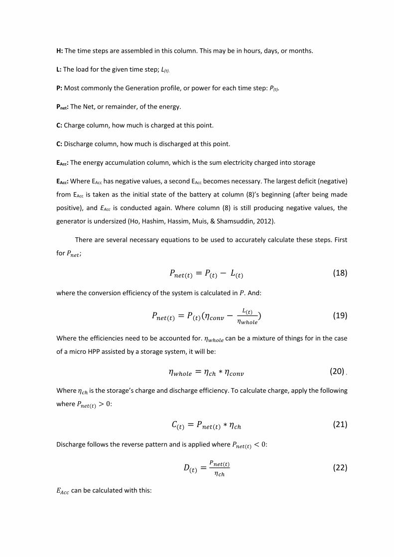
H: The time steps are assembled in this column. This may be in hours, days, or months.
L: The load for the given time step; L(t).
P: Most commonly the Generation profile, or power for each time step: P(t).
Pnet: The Net, or remainder, of the energy.
C: Charge column, how much is charged at this point.
C: Discharge column, how much is discharged at this point.
EAcc: The energy accumulation column, which is the sum electricity charged into storage
EAcc: Where EAcc has negative values, a second EAcc becomes necessary. The largest deficit (negative)
from EAcc is taken as the initial state of the battery at column (8)’s beginning (after being made
positive), and EAcc is conducted again. Where column (8) is still producing negative values, the
generator is undersized (Ho, Hashim, Hassim, Muis, & Shamsuddin, 2012).
There are several necessary equations to be used to accurately calculate these steps. First
for 𝑃𝑛𝑒𝑡;
𝑃𝑛𝑒𝑡(𝑡) = 𝑃(𝑡) − 𝐿(𝑡) (18)
where the conversion efficiency of the system is calculated in 𝑃. And:
𝑃𝑛𝑒𝑡(𝑡) = 𝑃(𝑡)(𝜂𝑐𝑜𝑛𝑣 − 𝐿(𝑡)
𝜂𝑤ℎ𝑜𝑙𝑒) (19)
Where the efficiencies need to be accounted for. 𝜂𝑤ℎ𝑜𝑙𝑒 can be a mixture of things for in the case
of a micro HPP assisted by a storage system, it will be:
𝜂𝑤ℎ𝑜𝑙𝑒 = 𝜂𝑐ℎ ∗ 𝜂𝑐𝑜𝑛𝑣 (20) .
Where 𝜂𝑐ℎ is the storage’s charge and discharge efficiency. To calculate charge, apply the following
where 𝑃𝑛𝑒𝑡(𝑡) > 0:
𝐶(𝑡) = 𝑃𝑛𝑒𝑡(𝑡) ∗ 𝜂𝑐ℎ (21)
Discharge follows the reverse pattern and is applied where 𝑃𝑛𝑒𝑡(𝑡) < 0:
𝐷(𝑡) =𝑃𝑛𝑒𝑡(𝑡)
𝜂𝑐ℎ (22)
𝐸𝐴𝑐𝑐 can be calculated with this:

62
𝐸𝐴𝑐𝑐(𝑡+1) = 𝐸𝐴𝑐𝑐(𝑡) + 𝐶(𝑡) + 𝐷(𝑡) (23)
Or with this:
𝐸𝐴𝑐𝑐(𝑡) = 𝐸𝐴𝑐𝑐(𝑡−1) + 𝐶(𝑡) + 𝐷(𝑡) (24)
Either form gives each step’s cumulative energy.
Where 𝐸𝐴𝑐𝑐(𝑇)is greater than 𝐸𝐴𝑐𝑐(𝑡=0), it is oversized, though the process won’t be repeated
if the 𝐸𝐴𝑐𝑐(𝑇)is within 10% of 𝐸𝐴𝑐𝑐(𝑡=0), (Ho, Hashim, Hassim, Muis, & Shamsuddin, 2012),
(Zahboune et al., 2016). Otherwise, the following equation is used to resize the turbine:
𝑆𝑇𝑛𝑒𝑤 = 𝑆𝑇𝐸𝐴𝑐𝑐(𝑇),− 𝐸𝐴𝑐𝑐(𝑡=0)
𝑇 (25)
Where 𝑇 is the total amount of time steps for the whole analysis (24 hours for a day etc.). If this is
a greater than 0.05% change, the suggest 𝑆𝑇𝑛𝑒𝑤 output is tested. The percentage change is
calculated here:
∆%=𝑆𝑇𝑛𝑒𝑤−𝑆𝑇
𝑆𝑇∗ 100 (26)
The process is continual repeated until the 𝑆𝑇𝑛𝑒𝑤 is less than 0.05% in change from the
current turbine. Once the final resizing has been found, the storage can be sized to the system using
the following equation (Zahboune et al., 2016):
𝑆𝑏𝑎𝑡𝑡 =𝐸𝐴𝑐𝑐(𝑀𝐴𝑋)
𝐷𝑂𝐷 (27)
Where the 𝐷𝑂𝐷 is the depth of discharge of the storage system.
4.3.2 Method Analysis:
The main point of comparison will be the final output of the two methods for sizing systems in this
research. The ESCA will not be carried out in as much detail here, as it requires many more inputs,
and individual time steps, to be analysed.
The same data profile was input for the sake of load terms, both just the initial domestic data,
and the combined load of the domestic and production load. The system’s DOD for hydroelectric
reservoirs is assumed to be 80%, as with Rozal, Alwi, Manan, Klemeš, & Hassan (2013). The
following gives the reservoir for the domestic load:
𝑆𝑟𝑒𝑠 =𝑅𝑒𝑠𝐴𝑐𝑐(𝑀𝐴𝑋)
𝐷𝑂𝐷 (28)

𝑆𝑟𝑒𝑠 =780,000
0.8= ~974,000
This means ESCA produces something of a larger figure than the 783,000l suggested by the original
analytical method. However, the 𝑅𝑒𝑠𝐴𝑐𝑐(𝑀𝐴𝑋) value of 780,000l is around 99.45% of the analytical
method’s output. This suggests that perhaps the main difference in the system is whether or not
they account for a system’s DOD value. Once again, the system never discharges from the reservoir,
as 𝐷𝑟𝑒𝑠is always zero, so water is only accumulated. This confirms the finding that in this case
storage is only necessary as a precautionary measure for peaking.
The combined load is calculated below using the findings of the ESCA process:
𝑆𝑟𝑒𝑠 =124,000
0.8= ~155,000
In this case, the final values are also very close. The analytical method’s output of 145,000l is 93%
of the ESCA adaptation output. However, this time it is the post DOD ESCA value that is within 10%.
However, 124,000l is still 86% of the analytical output, so is within 20%.
A suggestion to be made here is to simply substitute 𝑅𝑒𝑠𝐴𝑐𝑐(𝑀𝐴𝑋) from ESCA for 𝑆𝑟𝑒𝑞from
the analytical method in the 𝑆𝑟𝑒𝑠 calculation. This would give 980,000l for the initial, domestic only,
system, and 181,000l for the combined loads. These are still within the same percentage ranges, as
would be expected. Though the examples here suggest a similarity between the outputs, it is
noteworthy that ESCA’s reference to the system’s overall DOD may give it a slight edge in terms of
accuracy, which may also be provided by its deeper analysis of each time step in the year the system
runs for. It also suggests that both systems will return very similar results with the same data, and
that perhaps the analytical method should compensate for DOD. Finally, in both cases, the model
provided is not optimised for small scale use. ESCA, however, has the tools for resizing the
generator in each system through 𝑆𝑇𝑛𝑒𝑤 calculations. The analytical method is not designed to carry
this out, and may be used in combination with ESCA if necessary.
Both processes create considerably larger reservoir suggestions for the pure domestic load.
However, as it has been noticed, the reservoirs never discharged in the case study. This is likely a
result of the internal mathematics in each system. They are not adapted to account for unneeded
storage, so simply add up where there is no discharge, and create a larger system.

64
4.4 HOMER
4.4.1 Method Description
HOMER is, as discussed, a software which calculates the effective running of pre-assembled system
scenarios. The model is based on the recommendation of US Department of Energy’s NREL
(Alkababjie & Hamdon, 2012), and draws its data from NREL’s database (Matagira-Sánchez &
Irizarry-Rivera, 2015).
The system differentiates itself from the others described by virtue of being a software rather
than a manual calculation tool for planning purposes. The first step is to input a load, which in
HOMER is achieved by importing a time series file of kWh values. This can be either a 365-step input
of only day to day averages, or an 8760-step series for each hour (HOMER Energy - C, n.d.). The
software can also generate a load, which is based on the system’s internal NREL data. An area is
selected, as is a peak month, and HOMER will generate a believable household profile based on it’s
the regional data (HOMER Energy - C, n.d.). In either case a monthly average is supplied, which can
be adjusted alongside a series of sensitivity cases input by the user.
To meet the load supply, there is the option to create a generation system. The library
contains systems all renewable resource groups, including hydrogen, as well as an option for grid
input, and a series of generators which are based on both renewable and non-renewable resources.
There are also a series of storage options, including fuel cells, batteries, flywheels, and super
capacitors (HOMER Energy - C, n.d.). There are also key components like an AC/DC converter,
storage for hydrogen scenarios, and electrolysers for production (HOMER Energy - C, n.d.). Each
component can have its capital costs adjusted by the user at the creation point (HOMER Energy - C,
n.d.).
Whichever system is chosen, the resource can be input, be it hydro, hydrokinetic, biomass,
wind, solar or temperature. This leads to HOMER using a standard calculation for the potential of
the area, using this to calculate the system’s capability to generate electricity. The resources input
can also be adjusted to fit a series of sensitivity cases decided by the user. There is also the
possibility using online databases for the region selected (HOMER Energy - C, n.d.).
HOMER also functions to test the economic and environmental impacts of the system. When
setting up a project, the economics of the total system can be established. A project lifetime is
input, and so are capital costs, O&M and any potential penalties for capacity shortage, or emissions.
There are also inputs for potential discount rates and inflation rates (HOMER Energy - C, n.d.). It is
also possible to set project constraints, such as the minimum renewable fraction, and the maximum

allowable shortage, as well as the amount of “spare energy” that must be used to account for
fluctuations in the system. This includes having bridging energy available to meet sudden decreases
in intermittent resources, such as wind and solar (HOMER Energy - C, n.d.). Emissions data can then
be input, which takes the form of upper limits on outputs of typical power emissions, such as CO2
and particulate matter, and the penalty costs for outputting these systems (HOMER Energy - C,
n.d.). The final stage is the input of optimisation, which includes limits on the renewable
penetration of a system, and the battery autonomy, as well as other optimisation simulations the
software runs. The optimisation panel is key, as it calculates the NPVs of the system architecture
components, and ranks the results in increasing terms of NPC values after calculation.
The final output of HOMER’s calculation is a series of scenarios based on the proposed and
input architecture, as well as each load and resource sensitivity case. These scenarios will be the
feasible scenarios for meeting the required load, and there is a possibility that none are feasible
(HOMER Energy - C, n.d.). As noted above, there will be optimisation cases, which are ranked in
order based on their lowest NPC, as HOMER is a primarily economic algorithm model (HOMER
Energy - C, n.d.).
Other key functions of HOMER include the ability to scale up and down systems. If, for
example, you have previously estimated a 1MWh battery system for the site you wish to test in
HOMER, the input can be adjusted. There is an optimisation pane in the storage section that enables
a range of batteries to be tested by using and upper and lower limitation, which allows for results
that may show a feasible scenario with a lower battery value (HOMER Energy - C, n.d.).
4.4.2 Method Analysis
To supply examples for this analysis, an ESCA process was carried out based on the following load
and supply profile. This was generated to have a supply that over supplies one month and
undersupplies the next to test the size of the generation and storage. 3kW is the generated, and
each month requires either 2kW or 4kW.

66
Figure 13. Data generated for methodological debugging.
After completing the ESCA process, the 𝑆𝑇𝑛𝑒𝑤 output was a 3.382kW turbine, and a reservoir of
~1.09MWh, which would be roughly 7,598l water. Sensitivity cases of the load and the resource
(Geirlandsá river flows) increased by 10% and decreased by 10% were input. The turbine simulated
is shown in Figure 14, giving a near constant rate 3.382kW.
Figure 14. Turbine inputs in HOMER.
This is coupled with the reservoir, which has a round trip efficiency of 90%. The costs assumptions
are based on the existing costs in the HOMER library. An AC/DC converter with an efficiency of 85%
is included in this system.
0
0,5
1
1,5
2
2,5
3
3,5
4
4,5
13
26
65
19
76
13
01
16
26
19
51
22
76
26
01
29
26
32
51
35
76
39
01
42
26
45
51
48
76
52
01
55
26
58
51
61
76
65
01
68
26
71
51
74
76
78
01
81
26
84
51
KW
Time (Hours)
Debugging Data
Load (debug) Pconv

Figure 15. System Architecture in HOMER.
The resulting output suggests that each flow rate sensitivity case can only meet the lower (-
10%) sensitivity cases for the electrical load. In all cases, the reservoir is required. As the reservoir
input was created at the full 1.08MWh capacity, it was only tested at a range from 0 to 1. This
means that it could not be analysed for oversizing. However, this can be achieved by delving into
the results, where the method analysis will begin.
Looking first to the hydroelectric reservoir, it is noted that the optimisation results suggest it
was only discharged to a state of 60% at its lowest point across the year. This suggests a reservoir
of 40% the size, around 443kWh (3040l) may suffice. Looking to the turbine, it is shown to produce
around 3.31kW at a constant year-round production, which is unsurprising, and goes some way to
explaining why the lower sensitivity case load is the only one to be met. The total production is
roughly 29MWh, and 23.7MWh is consumed, and around 2.27MWh is produced in excess. The
hydro reservoir is established as having the highest costs in terms of capital, replacement, and
O&M. The total NPC is 93,846.61USD and the LCOE is 0.306USD.
HOMER gives considerably greater insight into the workings of a proposed system, but has
certain issues regarding its use. First, for the final outputs of the system to be accurate, a great deal
of pre-existing data must be collected. This would include accurate pricing of the components,
accurate knowledge of the resources and load, as well as an accurate idea of the probability for
fluctuation. Furthermore, NPC is reliant on an accurate discount rate being available, which may
not be the case. While a lot of this data is often available, it relies on the user having specific
components and system architecture in mind. This suggests that, unlike the previous methods, it is
more suited as a test simulation software for testing other methodology’s outputs. Not only this,
but the system requires previous knowledge of the hardware used, and, in reality, functions as an
algorithm test for case studies that the user has already created through other means. However, it
does have options for automatic sizing, which could be applied once the load and resource details
have been input by the user (HOMER Energy - C, n.d.). It is also to need a license purchased from
the company (HOMER Energy - B, 2016).

68
HOMER has the advantages of existing databases of components, a developed simulation,
and a combination of economic and technical feasibility outputs. However, it is more suited to
suggestions created through other means, than systems on its own. It is also a more technical tool
than other systems, and requires a license, so is a less accessible system than the previous
methodologies. This is likely because HOMER is a more flexible tool, and is not a system designed
for a singular use, such as storage sizing, potential analysis, or generation scale sizing.


70
5 Production Case Studies
5.1 Grid Resale
Having established a system that will supply a “spare” 10kW, without interruption, through use of
the 9kW wind turbine and micro HPP. This research will act under the assumption there is a surplus
a guaranteed 10kW generation to be sold to the grid.
Grid resale does not require any system beyond the initial generating turbines, as well as a
connection to the main Icelandic grid, which is assumed to be present. The sale statistics were
carried out under the assumption that the electricity for sale will sell for the same average USD/kWh
price as Landsvirkjun, Iceland’s major generation company, sells theirs. To gain the price in
USD/kWh, the data was taken from Landsvirkjun’s 2015 financial reports and performance reports.
This will be the price across the whole life span of the turbine and reservoir. This is assumed as
around 50 years, being the average of the 40 to 60-year life span range given by Chen et al. (2009),
Evans, Strezov, & Evans (2012), and Luo, Wang, Dooner, & Clarke, (2015). The following summary
operates under the following assumptions; The initial price gleaned from the Landsvirkjun data
remains constant across the life span, the system continues its 10kW generation for this time, the
yearly demand for sale will remain, and the system is assumed to run for 50 years, beginning from
2015, giving a total of 13 leap years (2016, 2020, 2024,2028, 2032, 2036, 2040, 2044, 2048, 2052,
2056, 2060, and 2064).
Table 7 Grid resale summary for proposed production. Source: (Landsvirkjun - B, 2016)
(Landsvirkjun - C, 2016).
Landsvirkjun 2015 energy sold 13.9 TWh
Landsvirkjun sales profits 2015 349,598,000USD
Landsvirkjun 2015 price per kWh 0.025USD/kWh
Proposed yearly generation 87.6MWh (87.84MWh for leap years)
Total for lifespan 4,383.12MWh

USD profit for proposed system life span 109,578USD
This is a relatively small amount, and may, in comparison to the final economic analysis of
the O&M costs, as well as capital, prove to not pay back the initial costs of the system. This will be
analysed in the economic summary chapter. Certainly, this is a surprisingly low return that may
not payback in full before after other costs are considered.
5.2 Hydrogen Production and Storage:
For the summary of hydrogen production and storage, data was gleaned from a series of existing
literature on the subject. As the system will be focused on continually providing 10kW, the focus
will be on producing hydrogen using electrolysis.
There are 3 electrolysis methods for the creation of hydrogen; proton exchange membrane
(hereafter PEM), high-temperature electrolysis (hereafter HTE), and alkaline electrolysis (hereafter
KOH) (Coskun, Akyuz, Oktay, & Dincer, 2011), (Abuşoğlu, Demir, & Özahi, 2016).
Valdés, Lucio, & Rodríguez (2013) is the first source focused on by this piece, as it gives the
equation to generate a useable power figure. Equation (29) is the equation, taken from Valdés,
Lucio, & Rodríguez (2013:
𝑃𝑈 = 𝜂𝑃𝑊𝐺 (29)
In the case of that research the 𝑃𝑊𝐺 is the efficiency of wind generation, including the amount
useable after conversion. In this paper, the useable wind generation was calculated using equation
(30):
𝑊𝐺𝑈 = 𝑊𝐺 ∗ 𝜂𝑐𝑜𝑛𝑣 (30)
Of course, this was combined with the hydroelectric conversion point, which must also be
considered in our case study, in equation (31), the 𝑃𝐻 value is the output of equation (1):
𝑃𝐻𝑈 = 𝑃𝐻 ∗ 𝜂𝑐𝑜𝑛𝑣 (31)
So, the combined 𝑃𝑈 is shown in equation (32):
𝑃𝑈 = 𝑊𝐺𝑈 + 𝑃𝐻𝑈 (32)
Which is the useable electricity for this entire system, specifically in this case for hydrogen
electrolysis.

72
For production rates, the literature focused on were the works of Coskun, Akyuz, Oktay, &
Dincer (2011), and Abuşoğlu, Demir, & Özahi (2016). Abuşoğlu, Demir, & Özahi (2016) gives the
process towards calculating the amount of electricity towards the creation of 1kg of Hydrogen. The
process taken from the research is as follows for that calculation:
𝑊𝑟𝑒𝑣𝑒𝑙𝑒𝑐𝑡 = 𝛥𝐺𝑒𝑙𝑒𝑐𝑡𝐻2𝑆
𝑀𝐻2 (33)
Abuşoğlu, Demir, & Özahi (2016) lists 𝛥𝐺𝑒𝑙𝑒𝑐𝑡𝐻2𝑂 and 𝛥𝐺𝑒𝑙𝑒𝑐𝑡𝐻2𝑆 as the Gibbs free energy
(kJ/kmol) of water and hydrogen sulphide, respectively, and 𝑀𝐻2as the molar mass of hydrogen
(kg/kmol). It then gives the following for the actual electricity used to create 1kg:
𝑊𝑎𝑐𝑡𝑒𝑙𝑒𝑐𝑡 = 𝑊𝑟𝑒𝑣𝑒𝑙𝑒𝑐𝑡
𝜂𝑡ℎ (34)
In this case, 𝜂𝑡ℎ is the thermal efficiency of the hydrogen electrolysis unit. These are the key
considerations for the creation of hydrogen with a consistent generation. For calculating 𝜂𝑡ℎ the
following is supplied:
𝜂𝑡ℎ = 𝐸∆𝐻
𝐸𝑐𝑒𝑙𝑙 (35)
Which is summarised to be as follows for both PEM and KOH:
𝜂𝑡ℎ = 1.48
𝐸𝑐𝑒𝑙𝑙 (36)
These calculations are can be used to create a conversion rate of electricity to hydrogen. In
the case of this research, a lot of the inputs used by the previous researches are unavailable. Also,
the input in equation (33) of 𝛥𝐺𝑒𝑙𝑒𝑐𝑡𝐻2𝑆 is not relevant to this research, as it is only relevant to
hydrogen sulphur alkaline electrolysis. The effect and role of hydrogen sulphide is not accounted
for in this research, as the data is unavailable. As a result, the systems in the case study were based
on the data of Coskun, Akyuz, Oktay, & Dincer (2011), and will be given in Nm3. The conversion of
energy to hydrogen measures are; 43-54% efficiency for HTE, resulting in a reading of 3.225kWh –
4.05kWh/Nm3, 55-75% for KOH systems, which is a result of 4.125 – 5.625kWh/Nm3, and 65-80%
for PEM, which results in 4.5 – 6KWh/Nm3. This means that PEM is the most efficient system, when
all sections of the process have been considered, despite having a lower production rate (Coskun,
Akyuz, Oktay, & Dincer, 2011).
Taking this case study’s available 10kW, the following tables summarise the potential for the
use of an electrolyser to create hydrogen from the proposed system. As above, the following

assumptions are carried over: The 10kW is available for the full life span, the system has the same
50-year life span, covering the same years, and the electrolyser’s efficiency remains across the life
span.
Table 8 Summary of HTE electrolysis production. Source: (Coskun, Akyuz, Oktay, & Dincer, 2011).
Yearly Generation (proposed MWh) 87.6MWh (87.84MWh leap year)
Total Life Span Generation (MWh) 4,383.12MWh
Yearly hydrogen production (Nm3) 21,629.63Nm3 – 27,162.8Nm3
(21,688.89Nm3 – 27,237.21Nm3)
Total life span hydrogen production (Nm3) 1,082,251.86Nm3 – 1,359,106.98Nm3
Table 9 Summary of KOH electrolysis production. Source: (Coskun, Akyuz, Oktay, & Dincer, 2011).
Yearly Generation (proposed MWh) 87.6MWh (87.84MWh leap year)
Total Life Span Generation (MWh) 4,383.12MWh
Yearly hydrogen production (Nm3) 15,573.33Nm3 – 21,236.36Nm3
(15,616Nm3 – 21,294.55Nm3)
Total life span hydrogen production (Nm3) 779,221.33Nm3 – 1,062,574.55Nm3
Table 10 Summary of PEM electrolysis production. Source: (Coskun, Akyuz, Oktay, & Dincer, 2011).
Yearly Generation (proposed MWh) 87.6MWh (87.84MWh leap year)
Total Life Span Generation (MWh) 4,383.12MWh
Yearly hydrogen production (Nm3) 14,600Nm3 – 19,466.67Nm3
(14,640Nm3 – 19,520Nm3)
Total life span hydrogen production (Nm3) 730,520Nm3 – 974,026.67Nm3
To convert to kilograms, the 11.126Nm3 to 1kg conversion rate for hydrogen is used
(Universal Industrial Gases, Inc., n.d.). This gives a range of 65,658.82kg to 122,155.94kg producible
across this system’s entire lifespan. Storage will take the form of a V174 canister, produced by
Dynetek, which has rough 174l capacity. Assuming the system is emptied yearly, the lowest PEM
production needs 100 canisters, while for the highest HTE production required 942 canisters. No
fuel cells will be used. This will be accounted for in the economic summary below.

74
However, it is noteworthy that none of these numbers are based on a specific production
case or technology. Fortunately, Young, Mill, & Wall (2007) makes reference to a company that
produces and electrolyser which functions in the 10kW range, the S40 (PES, 2016). The S40 can be
powered by up to 9.6kW, which is within the system’s uninterrupted production. The S40 is a PEM
system with a production rate of 6.7Nm2/kWh (PES, 2016). Assuming its use Table 9 describes its
potential production. Despite being a PEM system, and therefore the least productive above, PEM
is considered to be the most efficient system, in with the systems having the highest low and high
efficiency values in terms of energy input (Coskun, Akyuz, Oktay, & Dincer, 2011). Hence, this gives
the commercially available S40 for this level. It is also especially noteworthy that Coskun, Akyuz,
Oktay, & Dincer (2011) mentions PEM as the most efficient system after temperature management
and energy inputs. This makes it the most efficient in terms of round trip energy return.
Table 11 Summary of S40 PEM electrolysis production. Source: (PES, 2016).
Yearly Generation (proposed MWh) 87.6MWh (87.840MWh leap year)
Total Life Span Generation (MWh) 4,383.12MWh
Yearly hydrogen production (Nm3) 586,920Nm3 (588,528Nm3)
Total life span hydrogen production (Nm3) 29,366,904Nm3
This, assuming the same sales and extraction times as above, would require 4283 canisters, and
4295 during leap years. However, as these numbers are so high, there will also be a consideration
of each month being extracted and sold, requiring 357 or 358. This will be the system used for
economic summary below. In section 7.2.2, important discussions on the effect of storage and
compression in hydrogen will be considered.
5.3 Aluminium Smelting
Previous literature on aluminium smelting gives an operational temperature range of around 960C,
with the possibility for 373C running temperatures being possible (Schwarz, 2008), (Soares &
Oliveira, 2010). However, in the case of the lower temperature, is it merely a suggested system,
which may be used in future aluminium smelting uses. The range of operation is given to be roughly
100-350kA DC current, with 180kA being given as the desired current to maintain 960C temperature
within the aluminium smelting system (Schwarz, 2008), (Soares & Oliveira, 2010).
Growing from this data, an issue occurs; 180kA is generated with 43200kW at 240V, which is
the European standard used in Iceland (Soares & Oliveira, 2010). This is a continuous power value,

so the system here falls considerably short, as a 10kW is the useable energy, only 0.02% of the
required amount. This means that the case study could not support an independent aluminium
smelter. The case study will be adjusted to fit this limitation. The amount required to make a ton of
aluminium is given as 13MWh, so, where a functional system is supported, 1kWh can be assumed
to create 0.077kg of aluminium, or 77g (Schwarz, 2008).
Table 10 summarises the producible aluminium able to be produced using the consistent
10kW. As discussed, this system was unable to operate independently, so the table below is
assumed to be the result of an aluminium smelter buying the electricity for use from this site. The
values shown below will be the approximate aluminium produced with the case study’s
uninterrupted power. The same assumptions of continued 10kW production for the same 50-year
period, with no loss in efficiency, are taken again.
Table 12 Summary of potential aluminium production. Source: (Schwarz, 2008)
Yearly Generation (proposed MWh) 87.6MWh (87.840MWh leap year)
Total Life Span Generation (MWh) 4,383.12MWh
Yearly Aluminium production (kg) 6,745.2kg (6,763.68kg leap year)
Total life span aluminium production (kg) 337,500.24kg
5.4 Aquaponics and Hydroponics
Of these two systems, hydroponics is the older system, and aquaponics adds existing aquaculture
systems to hydroponics, creating a more efficient system with less waste and less water usage (Van
Ginkel, Igou, & Chen, 2017). There are two products of an aquaponics system; vegetables (or plants)
and fish, as fish are a key section of an aquaponics system (Forchino, Lourguioui, Brigolin, & Pastres,
2017).
The system proposed here will be an aquaponics system, for the reason that it has been
shown to have a more efficient return on electrical input than hydroponics in the research of Van
Ginkel, Igou, & Chen (2017). While both systems compared in that research have a comparable
yearly requirement, the aquaponics system produces the same amount of leafy greens with 0.017%
of the electricity, enabling it to produce more overall.
Using the case study production and generation data, a single aquaponics case study will be
created. Based on the life cycle assessment previously carried out by Forchino, Lourguioui, Brigolin,

76
& Pastres (2017), and the hydroponics study of Love, Uhl, & Genello (2015), the following makes up
the system architecture:
- A 70 W water pump, used to maintain water circulation.
- An aerator which is used across the year.
- A water heater to maintain water temperature. (as in Love, Uhl, & Genello (2015))
- A lighting system.
For the lighting, there will be a case which considers the use of an LX602C LED system, produced by
Heliospectra (Heliospectra, 2015). The initial greenhouse will be assumed to have an area of 40 m2,
as in Forchino, Lourguioui, Brigolin, & Pastres (2017). For all cases, it is assumed the internal
temperature will be maintained by external heating supply, either provided by the domestic load,
or imported in the form of heated water for space heating. In this case study, internal space heating
will not be considered. However, the maintenance of water temperature will be accounted for, as
an electrical water heater is used in colder months.
The water heater is noted to take most of the electrical load, and be mostly used in the winter
monthly peaks of the year (Love, Uhl, & Genello, 2015). In June, July, August, and September, the
system is said in Love, Uhl, & Genello (2015) to be almost entirely covered by heating from sunlight,
and not need a water heater. Therefore, the average electrical load for these months, 257.5kWh,
will be assumed to be the non-heating needs of the system, (the aerator, pump, and lighting). This
means the heating system will be an average total of 7,564kWh for the years studied, giving it a
2.43kW usage for hour each of the year. The 3,406kWh is the remainder, giving the remainder of
the system a power rating of around 0.16kW. The yearly kWh requirement for the system in Love,
Uhl, & Genello (2015) (10870kWh) will be assumed to have the same production rate as Van Ginkel,
Igou, & Chen (2017) (11545kWh), in terms of kWh/kg of produce. The electrical summary of the
system is seen in Table 11.
Table 13 Yearly electrical requirement for the example system. Source: (Love, Uhl, & Genello, 2015)
Water Heating Requirement (MWh) 7.56MWh
Other electrical Requirement (MWh) 3.41MWh
Total 10.87MWh
When introducing the LED system, a for need consistent artificial light the entire year is
assumed. The LX602C is designed for use in greenhouses, and each unit can cover 2m2 when hung
at a height of 2m. The system can run from 10.5W to 630W, and requires 2.6A current at 240V

(Heliospectra, 2015). For the proposed 40m2 site here, 20 LX602C hung at 2m will be needed.
Assuming they run for the year at 10.5W, they will require 91.98kWh. At 630W, they would require
5518.8kWh. The 116m2 site in Love, Uhl, & Genello (2015) is met by eight 40W bulbs, so a 40m2
could be covered by around three of the same. These run for around 10 hours per day, and 3650
hours in the year. So, of the 3406kWh above, the lighting requirement could be assumed to be
438kWh, giving the remainder as 2968kWh. The electrical requirement including the LX602C is
described in Table 12.
Table 14 Yearly electrical requirement for the example system with LED systems. Source: (Love, Uhl, &
Genello, 2015), (Heliospectra, 2015).
Water Heating Requirement (MWh) 7.56MWh
LED Requirement (kWh) 91.98kWh - 5518.8kWh
Non-lighting requirement (MWh) 2.97MWh
Total 10.62MWh – 16.05MWh
The final demand is outlined in Table 13, divided into the three scenarios. Once again, it is
based on the previous assumptions above in terms of production, efficiency, and operation period.
It is organised into three scenarios, depending on the lighting system implemented.
Table 15 Electrical requirement in relation to generation system proposed. Source: (Love, Uhl, & Genello,
2015), (Heliospectra, 2015).
40 W bulb LED system (10.5W) LED system
(630W)
Yearly Water Heating
(MWh)
7.56MWh 7.56MWh 7.56MWh
Lighting requirement
(kWh/MWh)
438kWh 91.98kWh 55.19MWh
Other requirement (MWh) 2.97MWh 2.97MWh 2.97MWh
Total requirement (MWh) 10.87MWh 10.6MWh 16.05MWh
Yearly generation (kWh) 87.6MWh
(87.84MWh)
87.6MWh
(87840kWh)
87.6MWh
(87.84MWh)

78
Proportion
(requirement/generation)
8.06 8.25 5.46
Assuming the requirements for the system remain consistent as they are upsized, the proposed
10kW generation system could support a system of 322.4m2 (original lighting system), 330m2(LED
at 10.5W consistently), and 218.4m2(LED at 603W consistently).
Assuming the larger scale systems are implemented, and that the upsizing has no effect on
the productivity of the system (i.e. the kWh/kg production is the same) Table 14 highlights how
much can be created with the system supported by this generator. The assumed produce of this
system is a variety of leafy greens, of which the average is taken (Van Ginkel, Igou, & Chen, 2017).
Table 16 Potential production in system proposed. Source: (Van Ginkel, Igou, & Chen, 2017).
Yearly Generation (proposed MWh) 87.6MWh (87.840MWh leap year)
Total Life Span Generation (MWh) 4,383.12MWh
Green Production Rate (kWh/kg) 0.6kWh/kg
Yearly Greens Production (kg) 52,560kg (52704kg)
Total Greens Production (kg) 2,629,872kg
Of all the cases proposed, this system has the highest production rate so far. Greens production is
shown to be achievable at this level. The assumption here is no fish production. However, for the
economic section of this research, a fish production rate scenario will be considered. As seen in
section 6.4, this will be based on multiplying the leafy green production rate by 0.08, the equivalent
cod production for 1kg of leafy greens (Forchino, Lourguioui, Brigolin, & Pastres, 2017).
5.5 Data Centres and Super Computers
To acquire a data centre that can be modelled against the available energy for use, it was first
necessary to look to existing data centres and their power profiles. The key thing to note is that
most existing systems require an uninterruptible power system (UPS), used to ensure the system is
consistently available (Iceland Meteorological Office, 2016), (Whitehead, Andrews, & Shah, 2015).
Therefore, the model of consistent 10kW power supply established for this case study will serve as
the system’s UPS.
Before developing the case to be tested here, there is the issue of cooling being the majority
load in most data centres. The large, data centre and super computer at KTH in Stockholm, has a

total load of 1,801MWh per month on average. This is shared across seven computers. Of this,
865MWh are given to the cooling of the system. However, the case study will be assumed to have
no mechanical cooling. This is based on the Icelandic Meteorological Office’s super computer, which
is noted to have no need for mechanical cooling systems due to the climate of Iceland (Iceland
Meteorological Office, 2016). As a result, an electrical load for cooling will be assumed to be
unnecessary at this site, particularly given the nature of having a reservoir of cold water available,
which could no doubt be used to assist in the cooling where necessary.
There are several measures that could be applied when it comes to considering the system
that is able to be supported by this generator. For example, both Whitehead, Andrews, & Shah
(2015) and Sevencan, Lindbergh, Lagergren, & Alvfors (2016) give values of the power requirement
for each of a system’s racks. These racks contain the ICT equipment used by a data centre or super
computer. These two systems give insight into the amount of racks that could be supported by the
case study, and thus give the useable system, in rack terms, a specific size. The contribution of these
systems will be given in terms of their memory usage, using Dual in-line memory modules (hereafter
DIMMs), which package memory (Intel, n.d.). 8 DIMMs of a capacity of 1GB are given as having a
power usage of 80W, so there will be an assumed 10W to 1GB memory usage for this case (Intel,
n.d.). The system outlined by Whitehead, Andrews, & Shah (2015) has a rate of 5kW/rack supplied.
This means each rack in the system has a potential storage and memory value of 500GB. For the
system described by Sevencan, Lindbergh, Lagergren, & Alvfors (2016), each rack has an installed
fuel cell with a rated capacity of 10kW. Assuming this capacity is after the fuel cell’s efficiency, this
would give each rack a memory capacity of 1TB.
Based on the assumptions above, a simple memory to kW conversion, is outlined in Table 15.
It does not necessarily account for the other sections of the system.
Table 17 Rack system summary for proposed production summary. Source: (Whitehead, Andrews, & Shah,
2015), (Sevencan, Lindbergh, Lagergren, & Alvfors, 2016), (Intel, n.d.).
Available production (proposed kW) 10kW
1GB production rate (kW) 0.01kW
Supported memory by system power (GB) 1,000GB
Rack power rating (kW) 5-10
Supported Racks 1-2

80
In this case, the generation can support a smaller super computer than those covered in the
literature. However, as with the aluminium smelting, it is not unlikely that this production site could
sell electricity for the sake of providing a UPS for a data centre or super computer’s use.
The second measure for converting power into a system would be in terms of the data centre
area. Multiple systems studied give a kW/m2 or kWh/m2, power or energy per area, measures. For
example, the 13MW system covered in Whitehead, Andrews, & Shah (2015) has a total space of
42,500m2, which gives it a rating of 306W/m2. However, it is noted that only 8110m2 of this system
is devoted to the computing use of the system (Whitehead, Andrews, & Shah, 2015), and that of
the 13MW required, 722kW are required for cooling, and only 12.895MW for the main server
system. Assuming an absence of mechanical cooling, this would give an equivalent system an area
requirement of 1.59kW/m2. Table 16 takes this measure and applies it to the case study.
Table 18 Summary based on UK 13MW data centre. Source: (Whitehead, Andrews, & Shah, 2015).
Available production (proposed kW) 10kW
Area production rate (kW/m2) 1.59kW/m2
Supported area by system power (m2) 6.29m2
The power supply assumptions for this scenario are as above, and the system is defined as a Tier III
data centre, which is a centre with low interruption and high availability, also characterised as
having individual components available for separate maintenance (OVH, n.d.), (Whitehead,
Andrews, & Shah, 2015).
Looking to different regions, Silicon Valley data centres are covered in the works of Mitchell-
Jackson, Koomey, Nordman, & Blazek (2003), with specific focus on a facility of 11,645m2. The
calculated power per m2 for this site was around 118W/m2, which is highly efficient, but accounts
for the entire building. The total given for the computing equipment is around 686kW, which makes
up around 2,555m2 of the site area. This means for pure computing systems, the 269W/m2 is the
power density per area for this particular site. The system’s productive capacity for a similar site is
listed below.
Table 19 Summary based on Silicon Valley 11645m2 data centre. Source: (Mitchell-Jackson, Koomey,
Nordman, & Blazek, 2003).
Available production (proposed kW) 10kW
Area production rate (kW/m2) 0.269kW/m2

Supported area by system power (m2) 37m2
The specific system is not given in terms of its processing power or tier, system. This means
production capacity cannot be commented on in this case.
Finally, a system in the projected production area will be looked to, in this case Iceland,
looking again to the computer system in use by the Iceland Meteorological Centre. The system used
here is four Cray XC30 systems, giving a system total of 15TB, with a computing value of 200TFLOPS
(tera floating points operations per second, a value of computer speed) (Iceland Meteorological
Office, 2016). An XC30 is made up of two cabinets, a compute cabinet and a blower cabinet which
take a total area of 94m2, and the entire system is around 188m2 (Cray, n.d.). The system has a total
power use is under 300kW. The power rating is therefore 1.6kW/m2, the summary is shown below
of the potential at the proposed site.
Table 20 Summary based on IMO data centre. Source: (Iceland Meteorological Office, 2016), (Cray, n.d.).
Available production (proposed kW) 10kW
Area production rate (kW/m2) 1.6kW/m2
Supported area by system power (m2) 6.25m2
The issue of above and the aluminium smelters is echoed again, however, as this is not a true
equivalency. The highest operating power capacity of the XC30 is 96kW (Cray, n.d.), and the system
here appears to require 75kW for each, as four are have a power rating below 300kW. This means
that the system proposed cannot generate electricity to run an equivalent system as at the IMO.
Once again, the site could sell electricity for the sake of providing a UPS for a data centre or super
computer’s use, as has been proposed previously.

82
6 Economic Summary
As seen in the methodology section, this economic summary will serve as a prospective guide to
potential products. It will only account for the pure profit returns against the initial capital cost,
and is missing key economic data. This means it does not serve as a wholly accurate payback
period, but more as a basis for the likelihood of economic return in each case study. The payback
periods in all cases are likely shorter than they would be with other data accounted for.
6.1 Grid Resale
The grid resale is based on the resale value proposed in the initial case study and outlined in Table
5 above, the resale value being 0.025USD/kWh, established above. The capital and O&M costs for
the grid resale case will be applied to all economic summary case studies.
The total system has a maximum possible output of around 25kW, giving the hydroelectric
turbine around 16kW capacity. Based on the lowest reading of the economic information available
would give the turbine a capital cost of around 40,000USD (Luo, Wang, Dooner, & Clarke, 2015).
The 21,106kWh reservoir, taken from the ESCA process, will have capital cost of 105,530USD (Luo,
Wang, Dooner, & Clarke, 2015). The O&M is 48USD/year for the turbine and 84.4USD/year for the
reservoir (Luo, Wang, Dooner, & Clarke, 2015). The O&M and capital costs of the wind turbine were
amalgamated into one, based on the 0.08USD/kWh given as the minimum LCOE given in
Ragnarsson, Oddsson, Unnthorsson, & Hrafnkelsson (2015), which is based on a 10% weighted
average capital costs. The value is 315,360USD, which will be counted once as a total capital cost in
this case.
The USD/kWh, based on the 0.025USD/kWh, does not cause the system lead to the system
paying back. Figure 15 depicts the system’s payback model.

Figure 16 Payback analysis for Grid Resale.
This shows that the USD 𝑅𝑛 never makes up in profit terms for the initial installation of the system.
Saved money is not accounted for. After extending the period by doubling it, this is still never paid
back, as it would seem to require an entirely new system at the end of the 50-year period.
6.2 Hydrogen Production and Storage
The hydrogen production economic model of the payback period is based on the S40 system that
is tested in the case study. This means it will be made up of an S40 electrolyser, which will need to
be replaced 4 times across the system (PES, 2016). The yearly O&M is given as being around
10.21USD/year, with replacement costs being ~55,000USD, based on the density price from
Abuşoğlu, Demir, & Özahi (2016). The storage will be handled by the V174 which have a
replacement cost of 3,544USD each (Young, Mill, & Wall, 2007). There will be a set of 358 V174s to
be used in this case, based on the monthly emptying schedule. The capital and replacement costs
will be 1,268,752USD and the O&M will be assumed as 0, as there is no mention in Young, Mill, &
Wall (2007). The V174 will be replaced every 10 years, the electrolyser every 13.
To find information on the sales return, Jón Björn Skúlason of Iceland New Energy was
consulted. Three sales return values were gained; were the hydrogen to be used in a refuelling
station, it would return 10EUR/kg, while it would return 200EUR/bottle in the current bottling and
sales market, New Energy will enter the market soon, at which point 50EUR/bottle is anticipated
(Skulason, 2017).
Figure 17 depicts the three situations based on the USD/kg, and USD/bottle values.
0
100000
200000
300000
400000
500000
Sum
of
Cn
-R
n
Year
Payback Analysis For grid resale

84
Figure 17 Payback Analysis for Hydrogen Production.4
As is observable, the most profitable system is the bottled system selling at the current rate.
However, the system is paid back in the third year in all cases.
6.3 Aluminium Smelting
As discussed in the case study, 10kW would not be likely to act as a continually consistent enough
supply to create a functioning aluminium smelter that could be run independently. As a result, the
economics of this situation will be based on the sale of energy to an aluminium smelting firm, as
opposed to the sale of created aluminium.
The value of the system is simply the original electricity generation only system, and the
resale price is taken as being, 0.035USD/kWh, the average price paid across the three main smelting
companies of Iceland (Askja Energy, 2015). Figure 18 depicts the pay back analysis.
-70000000
-60000000
-50000000
-40000000
-30000000
-20000000
-10000000
0
10000000
Sum
Cn
-R
n (
USD
)
Year
Hydrogen Payback Analysis
Refuel Station Payback Current Bottle Payback Future Bottle Payback

Figure 18 Payback Analysis for Aluminium.
The system is shown, like the grid resale system, to not meet a payback system, as the return is far
lower than the capital costs. However, unlike the grid resale only system, the system tends towards
repayment, rather than increasing in loss. In the grid resale case, the system consistently loses
money each year.
6.4 Aquaponics and Hydroponics
As based on the upper system, the aquaponics system is a 40m2 system with a series of 20 LED
based LX602C lights. This gives the system a capital cost of 8,240USD, based on the 206USD/m2
value in available literature (Bailey, Rakocy, Cole, & Shultz, 1997), while the LX602C has capital costs
at 37,000USD, as each unit is 1850USD (Growers House, n.d.). The O&M costs for the system is
around 4,334USD, none is listed for the LX620C. The only replaceable section of the system is the
light, which will be replaced 11 times over the 50-year lifespan (Heliospectra, 2015).
Return data will be based on the works of Bailey, Rakocy, Cole, & Shultz (1997), so 24 heads
of lettuce will be sold for 20USD, with each head being estimated at around 0.36kg. The system
used by Bailey, Rakocy, Cole, & Shultz (1997) has a fish output, so a fish sale estimate of 5.51USD/kg
is also considered. These were created by multiplying the kg of lettuce produce by 0.08, as the
equivalent amount made in fish terms according to Forchino, Lourguioui, Brigolin, & Pastres (2017).
The difference in fish breeds (trout and tilapia), is not accounted for in this analysis. Figure 19
displays the payback analysis.
0
50000
100000
150000
200000
250000
300000
350000
400000
450000
500000
Sum
Cn
-Rn
(U
SD)
Year
Payback analysis for Aluminium

86
Figure 19 Payback Analysis for Aquaponics.
As is shown in the figure, in both cases the system pays back sometime in the second year. This
means fish or lettuce sales would meet a payback period very quickly. Feed costs in both cases are
not accounted for.
6.5 Data Centres and Super Computers
The basis of the Data centre is a cross section of all the investigated case studies for the theoretical
production cases. The system’s capital costs will be 33,350USD based on the m2 supportable by the
system and the price of 5,302USD/kWh (Cray, n.d.), (Whitehead, Andrews, & Shah, 2015). The O&M
costs will be either 2,628USD and 2,635.20USD (for leap years), a result of the 0.03USD/kWh
supplied by Sevencan, Lindbergh, Lagergren, & Alvfors (2016). There is no information on lifetime
for components this system components, so all replacement will be assumed to be covered by O&M
costs.
The resulting system supports either one or two racks, which will be taken as equivalent to
existing rack systems operation in Iceland. Advania supplies a single rack for colocation purposes to
a client at a price of 990EUR/month. The following figure describes the payback period after the
original system, based on supplying the one rack or two rack system.
-2500000
-2000000
-1500000
-1000000
-500000
0
500000
Sum
Cn
-R
n (
USD
)
Year
Payback Analysis for Aquaponics
Payback all Payback lettuce

Figure 20 Payback analysis for the Data Centre.
After only supplying one rack, the system is not paid back across the life span. Two rack systems
would result in a 23-year payback period.
6.6 Economic Conclusion and Summary:
Three of the case studies are found to eventually payback; Data centres, aquaponics, and hydrogen
production. Data centres have the longest payback period at 23 years, while hydrogen pays back in
3. The aquaponics system is the fastest system to pay back, paying back within the second year at
an unspecified point.
Regarding systems that do not pay back, aluminium and grid resale, both systems tend
towards paying back before whole system must be replaced at the end of lifespan. This may be a
result of the micro level production of 10kW. Further research into a larger consistent power output
would establish the feasibility of a mixed-grid micro generator for resale purposes.
-800000
-600000
-400000
-200000
0
200000
400000
600000
Sum
Cn
-R
n (
USD
)
Year
Payback Analysis for Data Centres
Profit 1 Rack Profit 2 Rack

88
7 Conclusions and Discussion
7.1 Sensitivity Study
To create a series of sensitivity cases the load and hydroelectric water supplies were adjusted to
increase and decrease 10%. The supply cases were also applied to the original load, creating a sum
of 6 sensitivity cases to be investigated.
For the system’s application against the original data at a supply decrease of 10%, the system
begins at a shortage. To function consistently, 11,500l must be collected in the reservoir at the
beginning. However, a consistent supply of 9kW can be met feasibly in this sensitivity case. This
would decrease the production as follows: the grid resale and aluminium sale would be ~99,000
USD and ~138,000USD for their respective totals. Hydrogen production would be reduced to
~528,000Nm3 annually. ~2,377,000kg of leafy greens could be produced, along with 213,020kg of
trout, in the case of aquaponics. The Data centre would still be able to support one rack, at least,
or even the second rack assuming the 4kW Advania demand (Advania-B, n.d.).
When the decreased supply is set against the decreased load, the 9kW system is still able to
be met. It would run consistently with no initial gathering of water. It would maintain the stability
of a 9kW supply as above, and have the same production results.
The decreased supply against the increased load causes, as expected, a large shortage in the
end of the year. The initial contents of the reservoir would not need to be altered for consistent
running. However, without this, the system consistently outputs 8kW, which would support several
of these systems. Grid resale and aluminium power sale would be ~88,000USD and ~123,000USD
for their totals. Hydrogen production amounts to 470,000Nm3 annually. The aquaponics system
would produce ~2,104,000kg of leafy greens, along with ~190,000kg of trout. The Data centre
would still be able to support two racks, again in accordance with Advania’s numbers (Advania-B,
n.d.).
The increased supply set against the original domestic load resulted in a consistent supply
going up to 11.5kW becoming available. This requires an initial inflow of 18,300l. Assuming this

remains the case, the production cases are increased in this case to; ~126,000USD and
~176,000USD (grid resale and aluminium), ~675,000Nm3 (Hydrogen), ~3,024,000kg (greens,
aquaponics), ~272,000kg (trout, aquaponics), and no increase in supportable racks at a data centre.
This same supply against the decreased domestic load consistently produces an “extra”
12kW, with an initial state of ~31,000l. The resulting changes in output are as follows; ~132,000USD
and ~184,100USD (Aluminium and grid resale), ~704,000Nm3 (Hydrogen), ~3,156,000kg (greens),
284,00kg (trout), and the ability to add an extra rack per the Advania specifications for the data
centres (Advania-B, n.d.).
When the increased load is introduced, 10kW is once again given as the available useable
value, enabling the same results to be carried over from the initial case study.
7.2 Discussions
7.2.1 Case 1: Grid Resale
As is shown in the technical and economic case studies, grid resale is not considered to be a feasible
application of the generation profile. The initial capital without is not ever repaid within the
lifespan. This payback is based only on the current assumption of the sales price being
0.025USD/kWh, based on Landsvirkjun’s 2015 data. This may prove to inaccurate, as different
suppliers may sell for different prices, and the sales prices is assumed to be continually at that rate.
Also, as stated above, the payback period analysis method used in this research also doesn’t
account for the certain key economic criteria, such as inflation rates and energy price increase,
which leaves room for increased accuracy. Inflation rates and increased prices in electricity are not
only likely, but may serve as the difference between this system being repaid and remaining
unprofitable.
It is noteworthy, for example, that the system proposed has only been assessed based on
Landsvirkjun’s 2015 energy sales figures. This was after contacting the company itself, but no actual
real-world negotiation was made. Not only this, but a large amount of the production from major
energy companies is reserved for large scale energy intensive projects, so it is possible to speculate
that they do not expect to purely profit from their distribution of grid energy (Landsvirkjun - A, n.d.).
The case study also does not account for the saved money from buying energy for domestic
use, so misses one factor in the payback analysis. Nonetheless, it seems that simple resale of energy
would be a costly and unprofitable use of this micro generation.

90
7.2.2 Case 2: Hydrogen Production
Were any Hydrogen production electrolysis system to be used repayment is not only possible, but
so is profit. A PEM system is most profitable and is early to repay, as well as having the greatest
efficiency in terms of energy to production. This form of electrolysis is also the most likely to be
useable system with the 10kW consistent power supply, as the S40 system available required just
9.6kW. The other systems that are projected in the second case study, are unlikely to be supported
by the power produced.
There are certain other considerations in this case, such as the fact the production time of
each system needs to be calculated. The S40 system produces so much hydrogen that if the system
were to be sold on a yearly basis, the costs for the storage media would make it unlikely to be
repaid. This is seen in the economic analysis, which was based on the monthly sale to break even.
The next consideration here is that the 200EUR/bottle case is based on the current sales
price. This is influenced by high hydrogen import to Iceland making prices higher, hence the
50EUR/bottle value given by the local production company (Skulason, 2017). Also, the bottle size
was not given as a precise litre value, so there is a chance that the V174 is too large a product,
causing higher expenses. These two factors cast doubt on the current state of the hydrogen market
in Iceland, and thus question the capability to pay back for this case study to pay back.
Finally, the system required for bottling needs to be considered. The output pressure of an
S40 is about 13.8 bars. Dynetek’s v174s contain gas at a pressure of 350 bars (Young, Mill, & Wall,
2007). This casts doubt over the final output of the available energy for use, as the requirement for
a compressor is not accounted for. The data used for the compressor in Young, Mill, & Wall (2007),
is not available, so a key section of the analysis is questionable in this case study.
7.2.3 Case 3: Aluminium Smelting
The case for aluminium smelters produced the same result as grid resale, unable to meet the initial
capital demands in terms of sales profits and repayment. The system also tends towards zero.
However, as the entire system would have to be replaced at the life span’s end, even extending the
life span would not meet a repayment deadline.
There is an important consideration in this case, which is that there is a possibility that a
micro generator does not appear capable of maintain the current for an aluminium smelter. The
required kW range in available literature is far greater than 1MW, the upper limit supplied by Ion
& Marinescu (2011). This means that smelting aluminium operation at a micro generation level

cannot be feasibly achieved. This suggests that in both cases the aluminium smelter is a somewhat
infeasible production use for this case.
7.2.4 Case 4: Aquaponics and Hydroponics
An aquaponic system was modelled, and found to be sustainable by the case study. There are issues
with the system tested though; first, the value of the fish species sold did not necessarily equate to
that used in the economic comparison, as the literature sources provided distinct species. It is
outside the scope of this research to compare the full difference in farming conditions and spawning
habits of multiple fish species. Second, produce loss in these agricultural systems is also not
accounted for by this research.
The payback period is reliant on the existence of a market for the leafy greens produced by
this specific aquaponics system. The payback of the lettuce is reliant on 100% of the produced
lettuce being sold, which assumes a market for homegrown Icelandic lettuce, which may not be
present. Further research into the local vegetable market in general needs to be considered.
Finally, a system assuming no waste of creation, or lack of sales, as discussed, would not be
considered an accurate projection of the economic future of this investment. Nonetheless, the
aquaponics system appears to have the greatest production in comparison to energy input, and be
the least power intensive input.
7.2.5 Case 5: Data Centres and Super Computers
The case for super computers has several considerations to be listed. The first is to note that the
system appears to be downward scalable and deployable for sale. The system described would use
up to two racks of 5kW demand, though the one rack system would not pay back within the life
span.
However, there is potential for certain calculation errors using the available data. Assuming
the final economic analysis as the most feasible and likely case, which is reasonable, the capital
costs have the potential to be miscalculated. The capital costs were based on a kW/m2 of the Cray
XC30, which casts doubts on their validity, as the full-sized cabinet is a sold as a single unit, which
has a power requirement of 96kW. This suggests the exact kW/m2 is not necessarily accurate.
However, the ability to power racks in kW terms seen in Whitehead, Andrews, & Shah (2015) is
more likely. This also serves as the basis on the economic analysis. These systems are also sold at
the most readily available tariff, that of Advania’s, in the economic model. However, in many cases
the actual equivalency of these systems is questionable, as the racks themselves may not be
constructed of the same materials and equipment. Nonetheless, the rack power use of Advania’s

92
colocation services is given as around 4kW, so it is a useable example for this case study (Advania,
n.d.).
Finally, there is some disparity between available literature sources as to the actual service
provided. This is because the sources list their results in different formats. This suggests the need
for further insight and study into the actual useable product produced at a data centre, as many
are designed for certain uses (Advania-B, n.d.). However, it seems to be reasonable to assume that
the system provided would be classified as a tier 3 system, as it is based on the operating numbers
of several tier 3 sites.
7.2.6 Legal Considerations
Legal frameworks and restrictions are not considered for this research, but they are key to
understanding local obstacles to development. With regard to the size of HPPs considered by this
paper, little literature is currently available. However, there are summaries of the current master
plan for large scale projects, and the frameworks of those give insight into the considerations that
must be considered; the work groups of the plan were separated into Nature, Environment and
Cultural Heritage (work group 1), Recreation, Fishing, Hunting, and Agriculture (work group 2),
Social and Economic Impact, and Regional Development (work group 3), and a final group for
identification of future potential regions (Steingrímsson, Björnsson, & Adalsteinsson, 2007).
This means that when planning such a small-scale project as this, it is still likely necessary to
ensure there is not long-term negative environmental or cultural impact on the area developed.
Furthermore, the system’s effect on the local tourist and agricultural economics need to be
assessed to ensure there are no large negatives associated with this particular development. Finally,
at the time of writing, Steingrímsson, Björnsson, & Adalsteinsson (2007) made mention of
movements into phase 2 for the master plan, which included considerations for “small and mini”
HPPs, including an evaluation of the current protection value required. This would have major
implications for the legal permissions required for a micro-HPP project.
Although little concrete information on the legal requirements for a micro-HPP project is
available, current literature gives an outline to the required potential permissions. Though not
considered by this research, acquiring legal confirmation to move forward would affect several of
the planning phases outlined above, and likely provide a further cost to be considered for economic
analysis.

7.3 Conclusions
This study sought to explore the practical useable production gained form creating a micro
hydroelectric plant in combination with a single wind turbine, with a key focus on the effect of
applying a hydroelectric reservoir to ensure stability. An uninterruptible power supply system was
then created based on this stability. This was then used to answer the following research questions,
both technically and economically.
1. The first question was whether a mixed generation micro grid, based in Iceland, and backed
by a reservoir ESS, could be used to create a UPS. The case study that gives the production
of around 10kW “spare” electricity, after a singular domestic load, proves this to a
possibility. The combination of an intermittent wind production, a consistent hydroelectric
turbine production, and a reservoir to cover for production fluctuations in these systems,
was shown capable of this production. This case showed the advantages of hydroelectric
reservoirs at this scale, as they meet large discharge periods unmet by other ESS at this
scale. Their ability to store energy for a long time without loss, and operate for several days
at once, shows the worth of reservoirs at this scale.
2. The second question was of this case study’s ability to meet several agriculture and
industrial production scenarios. The production of several small scale industrial uses is
proven possible in 3 out of 5 cases studied. The power system is consistently able to meet
the production needs for the less intensive products. However, it is not able to make
something as power intensive as aluminium at this scale. However, for the sake of creating
aquaponic agricultural goods, hydrogen through electrolysis, and maintaining data centres,
the case study was shown to be effective and able to meet the needs of a several small-
scale case studies. The most productive in terms of goods produced was found to be
aquaponics lettuce produce.
3. What is Economic feasibility of each production scenario, in terms of pay back analysis?
Echoing the results of the previous question, the payback analysis confirmed that resale to
the grid, and sale to aluminium smelters would not become profitable or break even.
However, payback is confirmed in all other cases, in terms of profit. The sales of lettuce
alone, or lettuce in combination with fish, would repay the entire system, both electrical
and aquaponic. The sales of hydrogen would guarantee payback within the third year, and
would be profitable in the system if the current bottle prices remained. However, this is
unlikely (Skulason, 2017). Data Centres would payback, too, though it would require 2
racks, and take 23 years.

94
In summary, the suggested micro generation and storage system is shown to create a
constant and uninterrupted power supply. Importantly, this would be unachievable without the
system’s micro HPP reservoir. Not only this, but it is shown to be useable for creating small
scale production, using the power supply to create industrial or agricultural goods or services.
Furthermore, the system’s position in the wider question of the role of storage is shown to be
quite practical in terms of application, as it fits the geographical needs of a hydroelectric
system, and benefits from the physical advantages of reservoir ESS.
Further study is required in several areas, but a key starting point would be an upscaling of
the generated case study data, and the addition of a real-life turbine for the sake of producing
more reliable systems. For example, taking the original Geirlandsá monthly averages used, and
reducing them by a factor of 10, rather than 100, would give a range of 85kW to 185kW
production at any time. This would enable a consistent 120kW supply with no loss of power,
thanks again to the reservoir. There is a 100kW system suggested by Jawahar & Michael (2017),
which has an operational range of 40-100m, so the 60m useable point at the river could be
used. To consistently produce 100kW at this height, the 331l/s maximum flow is always
available, and the efficiency would be around 51%. This means a consistent 85kW could be
available the entire time for production purposes, which would have vast improvements on the
production rates.
The second area of further study would be into the specifics of each production scenario, as
to be more aware of the actual results in terms of production and payback. There is no
accounting for the system outside of the electrical terms, such as specific insight into the areas
of aquaponics and the computing make up of data centres. This is also the case for hydrogen
production systems to function. Each individual system would have to be tested in more specific
terms for clearer and fuller understanding. For the resale options, both to the grid, and to
smelters, research into a higher scale production system would be relevant, as noted in section
6.6. This could be carried out on HPPs producing up to the 1MW upper limit for the definition
of micro-HPPs.
Finally, as the losses to the 10kw output are incurred when the lower supply sensitivity cases
are applied, a more realistic reliable output should be the 8kW of those cases. This is to create
an economic buffer zone to account for these potential sensitivity losses.


96
References
Abdo, R. F., Pedro, H. T. C., Koury, R. N. N., Machado, L., Coimbra, C. F. M., & Porto, M. P.
(2015). Performance evaluation of various cryogenic energy storage systems. Energy, 90, Part
1, 1024–1032. https://doi.org/10.1016/j.energy.2015.08.008
Abuşoğlu, A., Demir, S., & Özahi, E. (2016). Energy and economic analyses of models
developed for sustainable hydrogen production from biogas-based electricity and sewage
sludge. International Journal of Hydrogen Energy, 41(31), 13426–13435.
https://doi.org/10.1016/j.ijhydene.2016.05.105
Advania. (n.d.). Standard Full Rack. Retrieved May 14, 2017, from
https://advania.com/datacenter/colocation/product/?itemid=62095a2e-37d1-11e6-9405-
005056bc0bdb
Advania-B. (n.d.). Data Centre Services. Retrieved May 14, 2017, from
https://advania.com/datacenter/colocation/#content
Alkababjie, M. F., & Hamdon, W. H. (2012). Feasibility and environmental effects study of
adding micro hydro power plant, converter and batteries to diesel generators using in
electrification a remote Iraqi village. In Engineering Sciences (FNCES), 2012 First National
Conference for (pp. 1–6). https://doi.org/10.1109/NCES.2012.6740475
Anderson, D., & Leach, M. (2004). Harvesting and redistributing renewable energy: on the role
of gas and electricity grids to overcome intermittency through the generation and storage of
hydrogen. Energy Policy, 32(14), 1603–1614. https://doi.org/10.1016/S0301-4215(03)00131-9
ArcGIS 10.4.1. (n.d.). World Hydro Reference Overlay.
Ashraf, M. M. (2014, October). Prosperity Through Power. Southasia, 18(10), 58–59.
Askja Energy. (2011, November 10). The Icelandic TSO. Retrieved May 14, 2017, from
https://askjaenergy.com/transmission/iceland-electricity-tso/

97
Askja Energy. (2015, August 18). Electricity tariffs to aluminum smelters in Iceland. Retrieved
May 10, 2017, from https://askjaenergy.com/2015/08/18/electricity-tariffs-to-aluminum-
smelters-in-iceland/
Bailey, D. S., Rakocy, J. E., Cole, W. M., & Shultz, K. A. (1997). Economic Analysis of a
Commercial - Scale Aquaponic System for The Production of Tilapia and Lettuce. In Tilapia
Aquaculture: Proceedings of the Fourth International Symposium on Tilapia in Aquaculture,
Orlando, Florida. Orlando. Florida.
Baker, J. (2008). New technology and possible advances in energy storage. Energy Policy,
36(12), 4368–4373. https://doi.org/10.1016/j.enpol.2008.09.040
Baños, R., Manzano-Agugliaro, F., Montoya, F. G., Gil, C., Alcayde, A., & Gómez, J. (2011).
Optimization methods applied to renewable and sustainable energy: A review. Renewable and
Sustainable Energy Reviews, 15(4), 1753–1766. https://doi.org/10.1016/j.rser.2010.12.008
Bloemendal, M., Olsthoorn, T., & Boons, F. (2014). How to achieve optimal and sustainable
use of the subsurface for Aquifer Thermal Energy Storage. Energy Policy, 66, 104–114.
https://doi.org/10.1016/j.enpol.2013.11.034
Boninella, M., Solheim, L., & Molinas, M. (2013). Hybrid micro grid feasibility study for the
Wawashang Complex in Nicaragua. In 2013 4th International Youth Conference on Energy
(IYCE) (pp. 1–8). https://doi.org/10.1109/IYCE.2013.6604182
Búrfellslundur EN - Búrfell Wind Farm. (2016, May 26). Retrieved May 26, 2016, from
http://burfellwindfarm.landsvirkjun.com/
Chade, D., Miklis, T., & Dvorak, D. (2015). Feasibility study of wind-to-hydrogen system for
Arctic remote locations – Grimsey island case study. Renewable Energy, 76, 204–211.
https://doi.org/10.1016/j.renene.2014.11.023

98
Chen, H., Cong, T. N., Yang, W., Tan, C., Li, Y., & Ding, Y. (2009). Progress in electrical
energy storage system: A critical review. Progress in Natural Science, 19(3), 291–312.
https://doi.org/10.1016/j.pnsc.2008.07.014
Coskun, C., Akyuz, E., Oktay, Z., & Dincer, I. (2011). Energy analysis of hydrogen production
using biogas-based electricity. International Journal of Hydrogen Energy, 36(17), 11418–
11424. https://doi.org/10.1016/j.ijhydene.2010.12.125
Cray. (n.d.). Cray XC30 -Brochure. Retrieved from
http://www.cray.com/Assets/PDF/products/xc/CrayXC30Brochure.pdf
Denholm, P., Ela, E., Kirby, B., & Milligan, M. (2010). The Role of Energy Storage with
Renewable Electricity Generation. NREL. Retrieved from
http://www.nrel.gov/docs/fy10osti/47187.pdf
Diaf, S., Belhamel, M., Haddadi, M., & Louche, A. (2008). Technical and economic
assessment of hybrid photovoltaic/wind system with battery storage in Corsica island. Energy
Policy, 36(2), 743–754. https://doi.org/10.1016/j.enpol.2007.10.028
Díaz-González, F., Sumper, A., Gomis-Bellmunt, O., & Villafáfila-Robles, R. (2012). A
review of energy storage technologies for wind power applications. Renewable and Sustainable
Energy Reviews, 16(4), 2154–2171. https://doi.org/10.1016/j.rser.2012.01.029
Divya, K. C., & Østergaard, J. (2009). Battery energy storage technology for power systems—
An overview. Electric Power Systems Research, 79(4), 511–520.
https://doi.org/10.1016/j.epsr.2008.09.017
Dursun, B., & Alboyaci, B. (2010). The contribution of wind-hydro pumped storage systems in
meeting Turkey’s electric energy demand. Renewable and Sustainable Energy Reviews, 14(7),
1979–1988. https://doi.org/10.1016/j.rser.2010.03.030
Earthship Biotecture. (2016, May 25). Earthship; Electricity. Retrieved May 25, 2016, from
http://earthship.com/Systems/electricity

99
Evans, A., Strezov, V., & Evans, T. J. (2012). Assessment of utility energy storage options for
increased renewable energy penetration. Renewable and Sustainable Energy Reviews, 16(6),
4141–4147. https://doi.org/10.1016/j.rser.2012.03.048
Forchino, A. A., Lourguioui, H., Brigolin, D., & Pastres, R. (2017). Aquaponics and
sustainability: The comparison of two different aquaponic techniques using the Life Cycle
Assessment (LCA). Aquacultural Engineering, 77, 80–88.
https://doi.org/10.1016/j.aquaeng.2017.03.002
Gil, A., Medrano, M., Martorell, I., Lázaro, A., Dolado, P., Zalba, B., & Cabeza, L. F. (2010).
State of the art on high temperature thermal energy storage for power generation. Part 1—
Concepts, materials and modellization. Renewable and Sustainable Energy Reviews, 14(1), 31–
55. https://doi.org/10.1016/j.rser.2009.07.035
Growers House. (n.d.). Heliospectra LX602C LED Grow Light for Sale - Reviews, Prices, &
More. Retrieved May 10, 2017, from http://growershouse.com/heliospectra-lx602-led-grow-
light
Hall, P. J., & Bain, E. J. (2008). Energy-storage technologies and electricity generation. Energy
Policy, 36(12), 4352–4355. https://doi.org/10.1016/j.enpol.2008.09.037
Heliospectra. (2015, July 28). The Fundamentals of Aquaponics and LED Grow Lights.
Retrieved April 28, 2017, from https://www.heliospectra.com/blog/fundamentals-aquaponics-
and-led-grow-lights
Ho, W. S., Hashim, H., Hassim, M. H., Muis, Z. A., & Shamsuddin, N. L. M. (2012). Design
of distributed energy system through Electric System Cascade Analysis (ESCA). Applied
Energy, 99, 309–315. https://doi.org/10.1016/j.apenergy.2012.04.016
HOMER Energy - B. (2016, June 1). HOMER Renewable Energy Microgrid Software |
Distributed Power and Microgrid Design Support. Retrieved June 1, 2016, from
http://www.homerenergy.com/software.html
100
HOMER Energy - C. (n.d.). HTML Help.
Hongpeechar, B., Krueasuk, W., Poungching-ngam, A., Bhasaputra, P., & Pattaraprakorn, W.
(2011). Feasibility study of micro hydro power plant for rural electrification in Thailand by
using axial flux permanent magnet. In Utility Exhibition on Power and Energy Systems: Issues
Prospects for Asia (ICUE), 2011 International Conference and (pp. 1–4).
https://doi.org/10.1109/ICUEPES.2011.6497732
Ibrahim, H., Ilinca, A., & Perron, J. (2008). Energy storage systems—Characteristics and
comparisons. Renewable and Sustainable Energy Reviews, 12(5), 1221–1250.
https://doi.org/10.1016/j.rser.2007.01.023
Ion, C. P., & Marinescu, C. (2011). Autonomous micro hydro power plant with induction
generator. Renewable Energy, 36(8), 2259–2267. https://doi.org/10.1016/j.renene.2011.01.028
Islam, M. R., Barua, S., & Barua, R. (2012). Feasibility Study of Micro-Hydro Power with an
Integrated Renewable Model in CHT. In 2012 IEEE Global Humanitarian Technology
Conference (GHTC) (pp. 160–165). https://doi.org/10.1109/GHTC.2012.34
Ja.is. (n.d.). Kort af Íslandi. Retrieved from
http://ja.is/kort/?q=pin%20%09%20Show%20Map%20%C3%81lftam%C3%BDri%2014%2C
%20108%20Reykjav%C3%ADkurborg%2C%20%C3%8Dsland
Jawahar, C. P., & Michael, P. A. (2017). A review on turbines for micro hydro power plant.
Renewable and Sustainable Energy Reviews, 72, 882–887.
https://doi.org/10.1016/j.rser.2017.01.133
Kalantar, M., & Mousavi G., S. M. (2010). Dynamic behavior of a stand-alone hybrid power
generation system of wind turbine, microturbine, solar array and battery storage. Applied
Energy, 87(10), 3051–3064. https://doi.org/10.1016/j.apenergy.2010.02.019

101
Kaldellis, J. K., Kavadias, K. A., & Spyropoulos, G. (2005). Investigating the real situation of
Greek solar water heating market. Renewable and Sustainable Energy Reviews, 9(5), 499–520.
https://doi.org/10.1016/j.rser.2004.04.006
Karakoulidis, K., Mavridis, K., Bandekas, D. V., Adoniadis, P., Potolias, C., & Vordos, N.
(2011). Techno-economic analysis of a stand-alone hybrid photovoltaic-diesel–battery-fuel cell
power system. Renewable Energy, 36(8), 2238–2244.
https://doi.org/10.1016/j.renene.2010.12.003
Kenisarin, M., & Mahkamov, K. (2007). Solar energy storage using phase change materials.
Renewable and Sustainable Energy Reviews, 11(9), 1913–1965.
https://doi.org/10.1016/j.rser.2006.05.005
Kipping, A. (2016, December 20). RE: Modelling and disaggregating hourly electricity
consumption in Norwegian dwellings based on smart meter data.
Kipping, A., & Trømborg, E. (2015). Hourly electricity consumption in Norwegian households
– Assessing the impacts of different heating systems. Energy, 93, Part 1, 655–671.
https://doi.org/10.1016/j.energy.2015.09.013
Kipping, A., & Trømborg, E. (2016). Modelling and disaggregating hourly electricity
consumption in Norwegian dwellings based on smart meter data. Energy and Buildings, 118,
350–369. https://doi.org/10.1016/j.enbuild.2016.02.042
Kondoh, J., Ishii, I., Yamaguchi, H., Murata, A., Otani, K., Sakuta, K., … Kamimoto, M.
(2000). Electrical energy storage systems for energy networks. Energy Conversion and
Management, 41(17), 1863–1874. https://doi.org/10.1016/S0196-8904(00)00028-5
Kusakana, K., Munda, J. L., & Jimoh, A. A. (2009). Feasibility study of a hybrid PV-micro
hydro system for rural electrification. In AFRICON 2009 (pp. 1–5).
https://doi.org/10.1109/AFRCON.2009.5308185

102
Landsvirkjun - A. (n.d.). Energy Products. Retrieved May 14, 2017, from
http://www.landsvirkjun.com/productsservices/energyproducts
Landsvirkjun - B. (2016). Consolidated Financial Statements 2015. Retrieved August 18, 2017,
from http://www.landsvirkjun.com/Media/financial-statements-20152.pdf
Landsvirkjun - C. (2016). Annual Report 2015. Retrieved August 18, 2017, from
http://annualreport2015.landsvirkjun.com/
Leadbetter, J., & Swan, L. (2012). Battery storage system for residential electricity peak
demand shaving. Energy and Buildings, 55, 685–692.
https://doi.org/10.1016/j.enbuild.2012.09.035
Li, C.-H., Zhu, X.-J., Cao, G.-Y., Sui, S., & Hu, M.-R. (2009). Dynamic modelling and sizing
optimization of stand-alone photovoltaic power systems using hybrid energy storage
technology. Renewable Energy, 34(3), 815–826. https://doi.org/10.1016/j.renene.2008.04.018
Love, D. C., Uhl, M. S., & Genello, L. (2015). Energy and water use of a small-scale raft
aquaponics system in Baltimore, Maryland, United States. Aquacultural Engineering, 68, 19–
27. https://doi.org/10.1016/j.aquaeng.2015.07.003
Luo, X., Wang, J., Dooner, M., & Clarke, J. (2015). Overview of current development in
electrical energy storage technologies and the application potential in power system operation.
Applied Energy, 137, 511–536. https://doi.org/10.1016/j.apenergy.2014.09.081
Maclay, J. D., Brouwer, J., & Samuelsen, G. S. (2006). Dynamic analyses of regenerative fuel
cell power for potential use in renewable residential applications. International Journal of
Hydrogen Energy, 31(8), 994–1009. https://doi.org/10.1016/j.ijhydene.2005.10.008
Mason, J. E., & Archer, C. L. (2012). Baseload electricity from wind via compressed air energy
storage (CAES). Renewable and Sustainable Energy Reviews, 16(2), 1099–1109.
https://doi.org/10.1016/j.rser.2011.11.009

103
Matagira-Sánchez, J. R., & Irizarry-Rivera, A. A. (2015). Feasibility study of micro pumped
hydro for integration of solar photovoltaic energy into Puerto Rico’s electric grid. In North
American Power Symposium (NAPS), 2015 (pp. 1–6).
https://doi.org/10.1109/NAPS.2015.7335192
Mitchell-Jackson, J., Koomey, J. G., Nordman, B., & Blazek, M. (2003). Data center power
requirements: measurements from Silicon Valley. Energy, 28(8), 837–850.
https://doi.org/10.1016/S0360-5442(03)00009-4
Mohanty, B. (2012, June). Reservoir. Education. Retrieved from
http://www.slideshare.net/bibhabasumohanty/reservoir-13443272
Nawri, N., Petersen, G. N., Bjornsson, H., Hahmann, A. N., Jónasson, K., Hasager, C. B., &
Clausen, N.-E. (2014). The wind energy potential of Iceland. Renewable Energy, 69, 290–299.
https://doi.org/10.1016/j.renene.2014.03.040
Nejranowski, P. (2011). Technical feasibility of the Mołstowa river energy utilization.
Retrieved from http://skemman.is/item/view/1946/7679
Orkustofnun. (n.d.). Listi yfir heimarafstodvar. Orkustofnun.
OVH. (n.d.). Tier 3/Tier 4: datacentre classification. Retrieved May 4, 2017, from
https://www.ovh.com/us/dedicated-servers/understanding-t3-t4.xml
Paish, O. (2002). Small hydro power: technology and current status. Renewable and
Sustainable Energy Reviews, 6(6), 537–556. https://doi.org/10.1016/S1364-0321(02)00006-0
Perez-Arriaga, I., Duenas-Martinez, P., & Tapia-Ahumada, K. (217AD). Electricity Security of
Supply in Iceland. MIT Energy Initiative. Retrieved from
https://energy.mit.edu/publication/electricity-security-supply-iceland/
PES. (2016). S Series Hydrogen Generation systems.

104
Pickard, W. F., Shen, A. Q., & Hansing, N. J. (2009). Parking the power: Strategies and
physical limitations for bulk energy storage in supply–demand matching on a grid whose input
power is provided by intermittent sources. Renewable and Sustainable Energy Reviews, 13(8),
1934–1945. https://doi.org/10.1016/j.rser.2009.03.002
Qureshi, W. A., Nair, N.-K. C., & Farid, M. M. (2011). Impact of energy storage in buildings
on electricity demand side management. Energy Conversion and Management, 52(5), 2110–
2120. https://doi.org/10.1016/j.enconman.2010.12.008
Ragnarsson, B. F., Oddsson, G. V., Unnthorsson, R., & Hrafnkelsson, B. (2015). Levelized
Cost of Energy Analysis of a Wind Power Generation System at Búrfell in Iceland. Energies,
8(9), 9464–9485. https://doi.org/10.3390/en8099464
Rahman, F., Rehman, S., & Abdul-Majeed, M. A. (2012). Overview of energy storage systems
for storing electricity from renewable energy sources in Saudi Arabia. Renewable and
Sustainable Energy Reviews, 16(1), 274–283. https://doi.org/10.1016/j.rser.2011.07.153
Rozal, N. E. M., Alwi, S. R. W., Manan, Z. A., Klemeš, J. J., & Hassan, M. Y. (2013).
Optimisation of Pumped-Hydro Storage System for Hybrid Power System Using Power Pinch
Analysis. Chemical Engineering Transactions, 35. Retrieved from
http://www.aidic.it/cet/13/35/014.pdf
Schwarz, H.-G. (2008). Technology diffusion in metal industries: driving forces and barriers in
the German aluminium smelting sector. Journal of Cleaner Production, 16(1, Supplement 1),
S37–S49. https://doi.org/10.1016/j.jclepro.2007.10.024
Sevencan, S., Lindbergh, G., Lagergren, C., & Alvfors, P. (2016). Economic feasibility study
of a fuel cell-based combined cooling, heating and power system for a data centre. Energy and
Buildings, 111, 218–223. https://doi.org/10.1016/j.enbuild.2015.11.012

105
Shukla, A. K., Venugopalan, S., & Hariprakash, B. (2001). Nickel-based rechargeable
batteries. Journal of Power Sources, 100(1–2), 125–148. https://doi.org/10.1016/S0378-
7753(01)00890-4
Skulason, J. B. (2017, November 5). Hydrogen Sales Costs Data.
Soares, F. M., & Oliveira, R. C. L. (2010). Modelling of temperature in the aluminium
smelting process using Neural Networks. In The 2010 International Joint Conference on
Neural Networks (IJCNN) (pp. 1–7). https://doi.org/10.1109/IJCNN.2010.5596645
Steingrímsson, B., Björnsson, S., & Adalsteinsson, H. (2007). MASTER PLAN FOR
GEOTHERMAL AND HYDROPOWER DEVELOPMENT IN ICELAND. Retrieved from
http://www.os.is/gogn/unu-gtp-sc/UNU-GTP-SC-04-19.pdf
Suberu, M. Y., Mustafa, M. W., & Bashir, N. (2014). Energy storage systems for renewable
energy power sector integration and mitigation of intermittency. Renewable and Sustainable
Energy Reviews, 35, 499–514. https://doi.org/10.1016/j.rser.2014.04.009
Suzuki, Y., Koyanagi, A., Kobayashi, M., & Shimada, R. (2005). Novel applications of the
flywheel energy storage system. Energy, 30(11–12), 2128–2143.
https://doi.org/10.1016/j.energy.2004.08.018
The Icelandic Meteorological Office. (2017). Delivery of data from the Hydrological database
(No. 2017–01–27/01).
Thornbloom, M., Ngbangadia, D., & Assama, M. (1997). Selected Proceedings of ISES 1995:
Solar World Congress. Part III Using micro-hydropower in the Zairian village. Solar Energy,
59(1), 75–81. https://doi.org/10.1016/S0038-092X(96)00096-5
Topographic Map; Iceland South. (2016, October 26). Retrieved October 26, 2016, from
http://en-gb.topographic-map.com/places/South-8088476/

106
Universal Industrial Gases, Inc. (n.d.). Hydrogen Unit Conversion (gas, liquid). Retrieved May
1, 2017, from http://www.uigi.com/h2_conv.html untitled - zotero://attachment/380/. (n.d.).
Retrieved from zotero://attachment/380/
Valdés, R., Lucio, J. H., & Rodríguez, L. R. (2013). Operational simulation of wind power
plants for electrolytic hydrogen production connected to a distributed electricity generation
grid. Renewable Energy, 53, 249–257. https://doi.org/10.1016/j.renene.2012.11.025
Van Ginkel, S. W., Igou, T., & Chen, Y. (2017). Energy, water and nutrient impacts of
California-grown vegetables compared to controlled environmental agriculture systems in
Atlanta, GA. Resources, Conservation and Recycling, 122, 319–325.
https://doi.org/10.1016/j.resconrec.2017.03.003
White, A. J. (2011). Loss analysis of thermal reservoirs for electrical energy storage schemes.
Applied Energy, 88(11), 4150–4159. https://doi.org/10.1016/j.apenergy.2011.04.030
Whitehead, B., Andrews, D., Shah, A., & Maidment, G. (2014). Assessing the environmental
impact of data centres part 1: Background, energy use and metrics. Building and Environment,
82, 151–159. https://doi.org/10.1016/j.buildenv.2014.08.021
Wind Power - The National Power Company of Iceland. (n.d.). Retrieved April 2, 2017, from
http://www.landsvirkjun.com/researchdevelopment/research/windpower
Wongphat, M., & Premrudeepreechacharn, S. (2015). Evaluation of engineering and economic
feasibility of micro-hydropower plant project. In 2015 5th International Youth Conference on
Energy (IYCE) (pp. 1–6). https://doi.org/10.1109/IYCE.2015.7180813
Yang, C.-J., & Jackson, R. B. (2011). Opportunities and barriers to pumped-hydro energy
storage in the United States. Renewable and Sustainable Energy Reviews, 15(1), 839–844.
https://doi.org/10.1016/j.rser.2010.09.020
Young, A. T. (2014). Hydrostatic Equilibrium and the Homogenous Atmosphere. Retrieved
January 4, 2017, from http://aty.sdsu.edu/explain/thermal/hydrostatic.html

107
Young, D. C., Mill, G. A., & Wall, R. (2007). Feasibility of renewable energy storage using
hydrogen in remote communities in Bhutan. International Journal of Hydrogen Energy, 32(8),
997–1009. https://doi.org/10.1016/j.ijhydene.2006.07.002
Zahboune, H., Kadda, F. Z., Zouggar, S., Ziani, E., Klemes, J. J., Varbanov, P. S., & Zarhloule,
Y. (2014). The new electricity system cascade analysis method for optimal sizing of an
autonomous hybrid PV/wind energy system with battery storage. In 2014 5th International
Renewable Energy Congress (IREC) (pp. 1–6). https://doi.org/10.1109/IREC.2014.6826962
Zahboune, H., Zouggar, S., Elhafyani, M., Ziani, M., & Dahbi, S. (2015). Optimal design
method for stand-alone solar system with LPSP technology by using electric system cascade
analysis method. In 2015 3rd International Renewable and Sustainable Energy Conference
(IRSEC) (pp. 1–6). https://doi.org/10.1109/IRSEC.2015.7454994
Zahboune, H., Zouggar, S., Yong, J. Y., Varbanov, P. S., Elhafyani, M., Ziani, E., & Zarhloule,
Y. (2016). Modified Electric System Cascade Analysis for optimal sizing of an autonomous
Hybrid Energy System. Energy, 116, Part 2, 1374–1384.
https://doi.org/10.1016/j.energy.2016.07.101
Zoulias, E. I., & Lymberopoulos, N. (2007). Techno-economic analysis of the integration of
hydrogen energy technologies in renewable energy-based stand-alone power systems.
Renewable Energy, 32(4), 680–696. https://doi.org/10.1016/j.renene.2006.02.005
Þórarinsdóttir, T. (2012). Development of a methodology for estimation of Technical
Hydropower potential in Iceland using high resolution Hydrological Modelling. Retrieved from
http://skemman.is/handle/1946/1076

108
Appendix
A1: Economic Summary Data
Price/kW used (USD) 2500
Price/kWh (USD) 5
O&M price for hydro turbine (USD) 48
O&M price for hydro reservoir (USD) 84.8
Wind O&M and Capital Amalgamation (USD) 0.08
Total generator capital costs (USD) 145,530
Estimated Sales Price (USD) 0.025
Estimated Aluminium Sales Price (USD) 0.035
Hydrogen bottle sales price current (EUR) 200
Hydrogen bottle sales price projected (EUR) 50
S40 O&M costs (USD) 0
Replacement costs v174 3,544
Refuel station price (USD/kg) 10
LX602C capital costs (USD/unit) 1850
Capital costs (based on area, USD) 8,240
Aquaponics O&M (USD) 4,334
Data centre capital costs (USD) 33,350
Data centre O&M 2,628 (2,635.20 leap years)
Tariff chard/month (EUR) 990

109
A2: Used Technology;
S40 (Source: (PES, 2016))
Power required (kW) 9.6
Output rate 1.05 Nm3/hr, 2.27 kg/24hr
kWh/kg production rate H2 (kWh/Nm) 6.7
Output Pressure (bars 13.8
Xinda Volute Axial Flow low head micro turbine generator (Source: (Jawahar & Michael,
2017))
Power capacity (kW) 10
Useable Head Range (m) 5-18
Flowrates useable (m3/s) 0.34 – 0.094
LX620C (Source: (Growers House, n.d.), (Heliospectra, 2015))
Power required (W) 10.5 - 630
Lifespan (hours) 50,000
Height hung 2m
Area covered 2m2