Micro Data For Macro Models

Fall 2009

Bad News/Good News

• Bad News

It is hard to get tenured at a top place

It is hard to publish

• Good News

Research productivity increases with effort

No one wins a Nobel Prize for their dissertation

1998 – 2000 Cohort At Top Schools (with likely omissions)Marianne Bertrand (Chicago) Ananth Seshadri (Wisconsin)

Esther Duflo (MIT) Amil Petrin (Minnesota)

Mike Greenstone (MIT) Muhamet Yildiz (MIT)

Emmanuel Saez (Berkeley) Markus Bruennermeier (Princeton)

Jonathan Levin (Stanford) Dmitriy Stoyarov (Michigan)

Sendhil Mullainathan (Harvard) Monika Piazzesi (Stanford)

Chang-Tai Hseih (Chicago) Ricardo Reis (Columbia)

Erik Hurst (Chicago) Dirk Krueger (Penn)

Enrico Moretti (Berkely) Martin Schneider (Stanford)

Luigi Pistaferri (Stanford) Mel Stephens (Michigan)

David Autor (MIT) Emre Ozdenoren (Michigan)

Mark Aguiar (Rochester) ~ 900 people got a Ph.D. from top 15

Marc Melitz (Harvard) departments during this time.

Victor Chevnozhakov (MIT)

Ted Miguel (Berkeley) ~ 30- 40 people got tenured at top place

Marco Battaglini (Princeton) ~ 4%-5% of students at top departments

David Lee (Princeton) get tenured at top departments

Publishing?

• The median Ph.D. from a top 20 department never publishes anything in a peer reviewed journal

• The median peer reviewed article has less than 15 citations.

• See Dan Hamermesh’s web site for:

“Young Economist’s Guide to Professional Etiquette”

http://www.eco.utexas.edu/faculty/Hamermesh/AdviceforEconomists.html

The Good News

• The creation of research is a skill just like inverting a matrix, solving DSGE models, computing standard errors, etc.

• The more you work on it, the better you will become.

• Read the early work of those recently tenured at top schools. Every single one of you could have written the same papers!

It is not our technical prowess that distinguishes us throughout our careers, it is our ability to innovate.

Those who have impact on the profession due so because of their ideas.

Question: Which Style of Research Is Best?

• Style is not as important as substance.

Structural vs. Reduced Form?

Theory vs. Empirics?

Partial Equilibrium vs. General Equilibrium?

• Perfect example: The work of Kevin Murphy

What Skill Are New Ph.D’s Most Deficient?

• Having the ability to identify interesting research questions

• The confusion of theoretical or empirical fire power as being an “end” as opposed to a “means”.

• Not having the ability to explain why anyone would care about their research.

The Main Goal of This Class

• Get you to think about “questions” as opposed to “models”.

• Caveat: Models are good!

You all have strong skills in this dimension.

• My comparative advantage is in questions.

• My style should be a complement – not a substitute – to your existing skill set.

Additional Goals

• Introduce you to a models and literature focusing on household financial behavior which are of interest to macro economists broadly defined:

consumption, saving, inequality, housing, labor supply, entrepreneurship, default, etc.

• Introduce you to micro data sets which can shed light on these questions.

• Focus on papers that have had big impacts on the respective literatures – nearly all of which could have been written by anyone in this class (with your existing skill sets).

Some Housekeeping….

• Homework

Three components

Expectation for auditors

• T.A.

• Papers

• Slides

• Timing

Lastly

• Discussion about the process of research is highly encouraged.

• I will often ask you how you would attempt to solve certain research questions.

• I may not have the answers myself.

• The dialog is part of the research process.......

Lecture 1:Consumption

Weeks 1 and 2: Consumption

• Why is it important?

- Learn about household preferences broadly

C.E.S. vs. log vs. other / Habits? / Status?

- Estimate preference parameters

intertemporal elasticity of substitution/ risk aversion/ discount rate

- Learn about income process

permanent vs. transitory shocks / expected vs. unexpected

- Learn about financial markets/constraints

liquidity constraints / risk sharing arrangements

- Learn about policy responses

spending after tax rebates, fiscal multipliers, etc.

Weeks 1 and 2: Consumption

• The big picture with consumption:

- Use estimated parameters to calibrate models

- Understand business cycle volatility

- Conduct policy experiments (social security reform, health care reform, tax reform, etc.)

- Estimate responsiveness to fiscal or monetary policy

- Broadly understand household behavior

Weeks 1 and 2: Consumption

• The outline of this lecture:

- Understand lifecycle consumption movements (this week)

o Illustrative of how one fact can spawn multiple theories.

o Show how a little more data can refine the theories

o Illustrate the empirical importance of the Beckerian consumption model (i.e, incorporating home production and leisure).

Weeks 1 and 2: Consumption

• The outline of this lecture:

- Discuss the importance of precautionary savings (next week)

- Discuss the estimation of household preference parameters (next week)

- Discuss the use of consumption data to estimate the income process households are facing (next week)

- Discuss changes in inequality over time (next week)

- Discuss evidence on household risk sharing (next week)

- Discuss testing for alternative specifications of household preferences (next week)

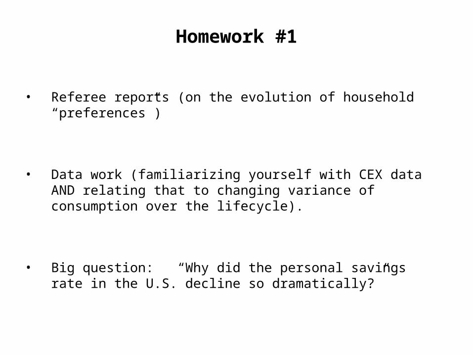
Homework #1

• Referee reports (on the evolution of household “preferences”)

• Data work (familiarizing yourself with CEX data AND relating that to changing variance of consumption over the lifecycle).

• Big question: “Why did the personal savings rate in the U.S. decline so dramatically?”

Why start with consumption

• Much better micro data on the household sector

(Consumption and labor supply)

• Less good data on the firm side

• International data is becoming more prevalent (trade data)

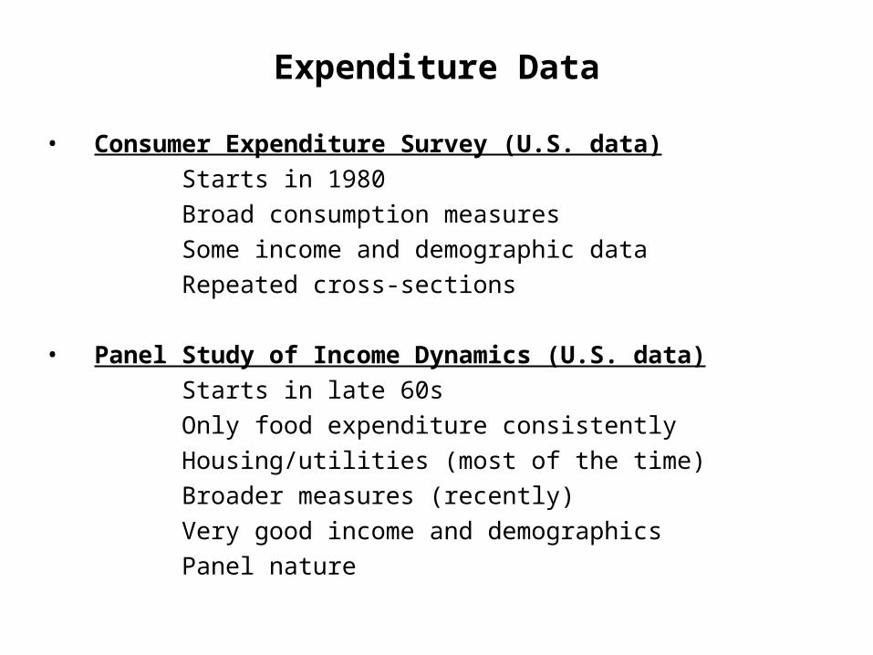
Expenditure Data

• Consumer Expenditure Survey (U.S. data)

Starts in 1980

Broad consumption measures

Some income and demographic data

Repeated cross-sections

• Panel Study of Income Dynamics (U.S. data)

Starts in late 60s

Only food expenditure consistently

Housing/utilities (most of the time)

Broader measures (recently)

Very good income and demographics

Panel nature

Expenditure Data

• British Household Panel

• Family Expenditure Survey

• Bank of Italy Survey of Household Income and Wealth

• There are others….

Fact 1: Lifecycle Expenditures

Plot: Adjusted for cohort and family size fixed effects

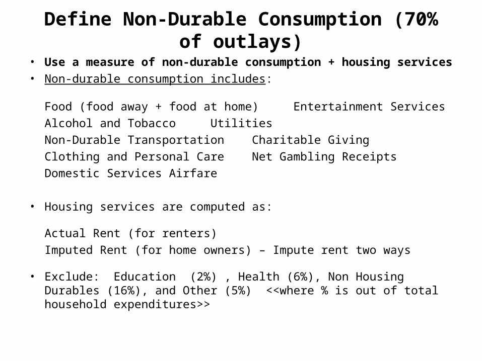
Define Non-Durable Consumption (70% of outlays)

• Use a measure of non-durable consumption + housing services

• Non-durable consumption includes:

Food (food away + food at home) Entertainment Services

Alcohol and Tobacco Utilities

Non-Durable Transportation Charitable Giving

Clothing and Personal Care Net Gambling Receipts

Domestic Services Airfare

• Housing services are computed as:

Actual Rent (for renters)

Imputed Rent (for home owners) – Impute rent two ways

• Exclude: Education (2%) , Health (6%), Non Housing Durables (16%), and Other (5%) <<where % is out of total household expenditures>>

Empirical Strategy: Lifecycle Profile of Expenditure

• Estimate:

(1)

where is real expenditure on category k by household i in year t.

Note: All expenditures deflated by corresponding product-level NIPA deflators.

Cohortit = year-of-birth (5 year range – i.e., 1926-1930)

Dt = Vector of normalized year dummies (See Hall (1968))

Family Composition Controls:

Household size dummies, Number of Children Dummies

Marital status dummies , Detailed Age of Children Dummies

kitC

0ln( )k kit age it c it t t fs it itC Age Cohort D Family

Fact 2: Hump Shaped Profile – By Education

From Attanasio and Weber (2009)

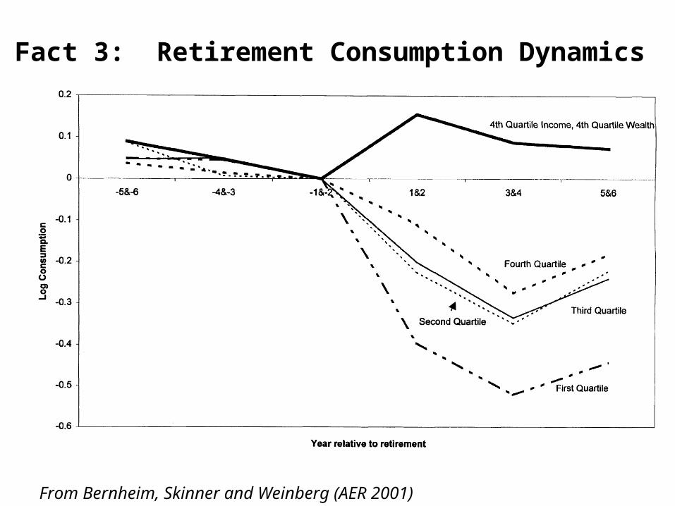
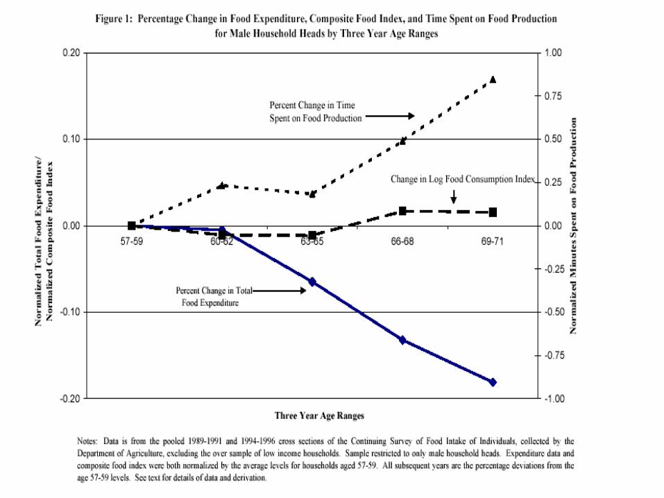
Fact 3: Retirement Consumption Dynamics

From Bernheim, Skinner and Weinberg (AER 2001)

The Puzzle? (Friedman, Modigliani, Hall, etc.)

( )

1

1max ( , ) ( , )

1t

s tT

t t t s sC

s t

u C E u C

1 1 1(1 )( )t t t t tX r X C Y

t t tY PV

1t t tP g P N

{Nt, Vt} are permanent and transitory mean zero shocks to income with underlying variances equal to σ2

N and σ2V

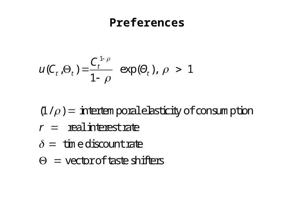
Preferences

1

( , ) exp( ), 11

(1/ ) intertemporal elasticity of consumption

real interest rate

time discount rate

vector of taste shifters

tt t t

Cu C Θ

r

Euler Equation

*1 11 1

1 1

*

ln(1 ) ( )ln(1 )

ln ln

if (in all periods) or if they are constant and

if the forecast error of future consumption (embedded in ) is constant

then cons

t t tt t

t t t

rC

where C C C

r

umption growth only depends on changes in tastes ( )

or changes in the real interest rate.

What Are Potential Taste Shifters Over Life Cycle

1. Family Size

o Makes some difference

o Hump shaped pattern still persists

o See Facts 1 and 3 (above) – these were estimated taking out detailed family size controls.

2. Other Taste Shifters (that change over the lifecycle – for a given individual)?

Questions:

What Else Drives the Hump Shaped

Expenditure Profile?

Why Does Expenditures (on food)

Fall Sharply At Retirement?

Explanations

• Non-Separable Preferences Between Consumption and Leisure - Heckman (1974)

• Liquidity Constraints and Impatience - Gourinchas and Parker (2002)

• Myopia - Keynes (and others)

• Time Inconsistent Preferences (with liquidity constraints) - Angeletos et al (2001)

• Habits and Impatience

• Home Production/Work Related Expenses - Aguiar and Hurst (2005, 2008)

Non-Separable Consumption and Leisure

( )

,1

1 1

*1 0 1 1 2 1 1

1max ( , ) ( , )

1

1( , ) ( (1 ) )

1

ln(1 ) (1 )

t t

s tT

t t t s sC N

s t

t t t t

t t t t

u C N E u C N

u C N C N

C r N

Testing Non-Separable Consumption and Leisure

Isolate Spending Changes Around Retirement

Aguiar and Hurst “Consumption vs. Expenditure” (JPE 2005)

34

Data: Measuring Consumption Directly

• Main Data Set: Continuing Survey of Food Intake of Individuals (CSFII)

– Conducted by Department of Agriculture– Cross Sectional / Household Level Survey– Two recent waves: Wave 1 (1989 -1991) ; Wave 2 (1994-1996)– Nationally Representative– Multi Day Interview– All individuals within the household are interviewed (C at individual level)– Tracks final food intake (not intermediate goods --- think about a cake)

• Detailed food expenditure, demographic, earnings, employment, and health measures

• Large sample sizes:

– 6,700 households in CSFII-91– 8,100 households in CSFII-96

35

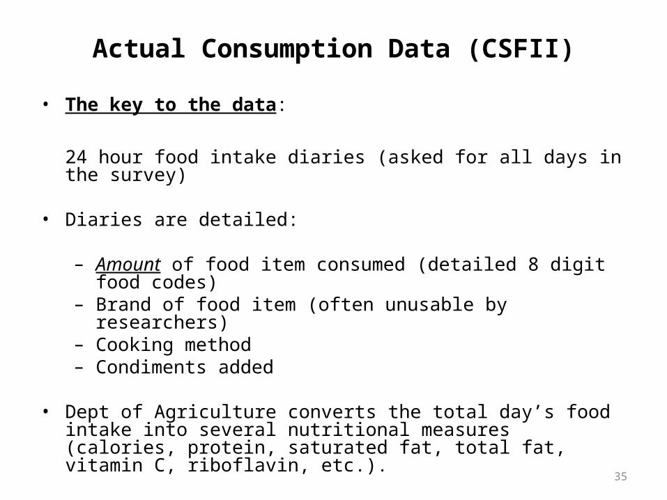
Actual Consumption Data (CSFII)

• The key to the data:

24 hour food intake diaries (asked for all days in the survey)

• Diaries are detailed:

– Amount of food item consumed (detailed 8 digit food codes)– Brand of food item (often unusable by researchers)– Cooking method– Condiments added

• Dept of Agriculture converts the total day’s food intake into several nutritional measures (calories, protein, saturated fat, total fat, vitamin C, riboflavin, etc.).

– The conversion is made using all food diary data (i.e., brand, whether cooked with butter).

36

8 digit food codes: Cheese• Example 18 of the 100 8-digit codes for cheese.

14101010 CHEESE, BLUE OR ROQUEFORT

14102010 CHEESE, BRICK

14102110 CHEESE, BRICK, W/ SALAMI

14103020 CHEESE, BRIE

14104010 CHEESE, NATURAL, CHEDDAR OR AMERICAN TYPE

14104020 CHEESE, CHEDDAR OR AMERICAN TYPE, DRY, GRATED

14104200 CHEESE, COLBY

14104250 CHEESE, COLBY JACK

14105010 CHEESE, GOUDA OR EDAM

14105200 CHEESE, GRUYERE

14106010 CHEESE, LIMBURGER

14106200 CHEESE, MONTEREY

14106500 CHEESE, MONTEREY, LOWFAT

14107010 CHEESE, MOZZARELLA, NFS (INCLUDE PIZZA CHEESE)

14107020 CHEESE, MOZZARELLA, WHOLE MILK

14107030 CHEESE, MOZZARELLA, PART SKIM (INCL ""LOWFAT"")

14107040 CHEESE, MOZZARELLA, LOW SODIUM

14107060 CHEESE, MOZZARELLA, NONFAT OR FAT FREE

37

Changes in “Spending” At Retirement

Run: ln(xi) = γ0 + γ1 Retiredi + γ2 Zi + errori

• Retiredi is a dummy variable equal to 1 if the household head is retired.

• Instrument Retiredi status with age dummies (potential endogeneity)

• Z includes: race, sex, health, region, time, family structure controls

• Sample: Relatively “young” older households: Heads aged 57-71

• Total food expenditure (x) falls by 17% for retired households (γ1), p-value < 0.01

• Other results:

– Food expenditure at home falls by 15%

– Food expenditure away from home falls by 31%

38

Changes in “Consumption” at Retirement

• How do we turn these food diaries into meaningful measures of consumption?

• Our approach:

1. Examine Nutritional Quality of Diet (vitamins, cholesterol, fat, calories, etc.)

2. Examine individual goods with strong income elasticities (hotdogs, fruit, yogurt, shellfish, wine)

3. Luxury/Quality goods (e.g. brands vs generics, lean vs. fatty meat)

4. Use structural model to aggregate food consumption data and perform formal PIH test.

39

Nutritional Measures• Regress: ln(ci) = α0 + α1 ln(yperm) + demographics <<sample: heads 25-55>>

• Regress: ln(ci) = β0 + β1 Retired + demographics <<sample: heads 57-71>>

Consumption Measure (in logs) Estimated Elasticity (α1) Retirement Effect (β1)

Calories -4% (2%) -2% (4%)

Protein * -1% (1%) -3% (2%)

Vitamin A * 44% (5%) 36% (9%)

Vitamin C * 34% (5%) 33% (9%)

Vitamin E * 18% (3%) 11% (4%)

Calcium * 10% (2%) 13% (4%)

Cholesterol * - 26% (3%) -9% (5%)

Saturated Fat * - 9% (2%) -7% (3%)

• * Includes log calories as an additional control ; Include supplements as an additional control.

• Instrument for retirement status with age; Examined non-linear specifications (not reported)

• No evidence of any deterioration in diet quality

40

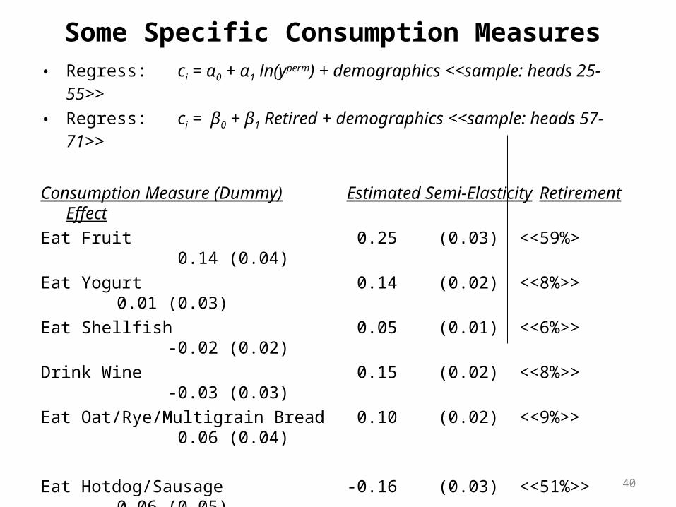
Some Specific Consumption Measures• Regress: ci = α0 + α1 ln(yperm) + demographics <<sample: heads 25-55>>

• Regress: ci = β0 + β1 Retired + demographics <<sample: heads 57-71>>

Consumption Measure (Dummy) Estimated Semi-Elasticity Retirement Effect

Eat Fruit 0.25 (0.03) <<59%> 0.14 (0.04)

Eat Yogurt 0.14 (0.02) <<8%>> 0.01 (0.03)

Eat Shellfish 0.05 (0.01) <<6%>> -0.02 (0.02)

Drink Wine 0.15 (0.02) <<8%>> -0.03 (0.03)

Eat Oat/Rye/Multigrain Bread 0.10 (0.02) <<9%>> 0.06 (0.04)

Eat Hotdog/Sausage -0.16 (0.03) <<51%>> -0.06 (0.05)

Eat Ground beef -0.10 (0.03) <<22%>> -0.01 (0.04)

• Sample means in << >>

• Instrument for retirement status with age

• Drawback: Tastes could differ across income types

• Drawback: Categories are broad and do not allow for differences in quality

41

Luxury Goods/Quality: My Favorite….

• Examine some dimensions of quality:

– Eating at restaurants with Table Service

– Eating Branded vs. Generic Goods

– Eating Lean vs. Fattier Cuts of Meat

• Restaurants, Brands, and Eating Lean Meat have very STRONG income elasticities in the cross section of working households.

• If households are unprepared for retirement, we should see them switching away from such consumption goods.

• No evidence of that in the data.

42

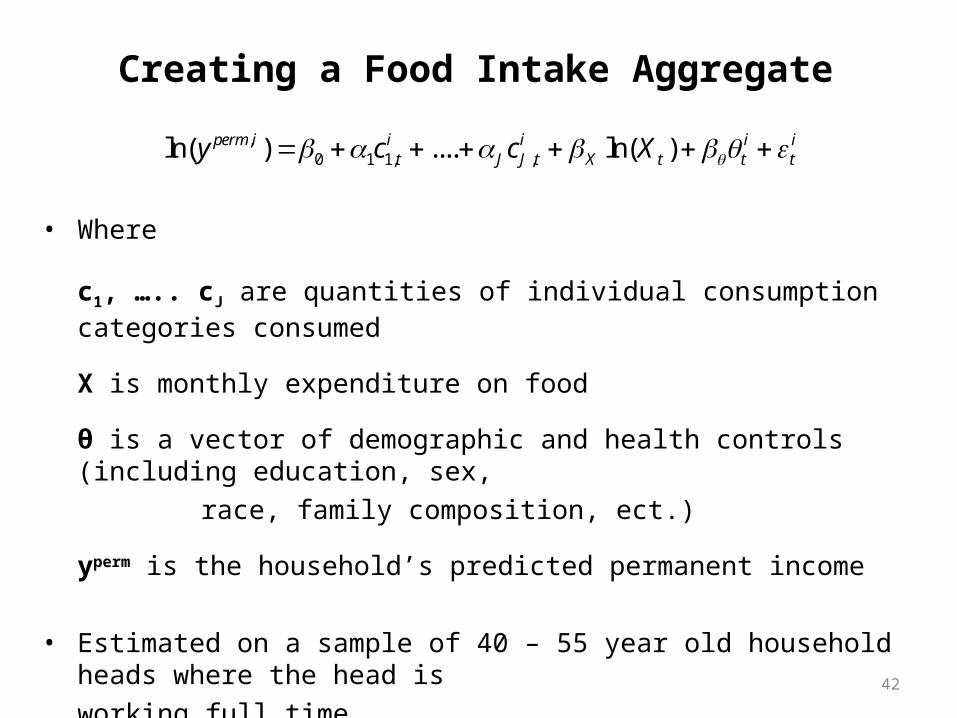
,0 1 1, ,ln( ) .... ln( )perm i i i i i

t J J t X t t ty c c X

• Where

c1, ….. cJ are quantities of individual consumption categories consumed

X is monthly expenditure on food

θ is a vector of demographic and health controls (including education, sex,

race, family composition, ect.)

yperm is the household’s predicted permanent income

• Estimated on a sample of 40 – 55 year old household heads where the head is

working full time.

Creating a Food Intake Aggregate

43

• Permanent income is our numeraire – one unit increase in our consumption index maps into a one percent increase in permanent income.

– What are we doing: We project permanent income of household i onto household i’s consumption (controlling for taste shifters).

• Basically, in a statistical sense, if you tell me what you eat, I can predict your permanent income. Our consumption index is in permanent income dollars!

• We also did this for households aged 25-55 who are working fulltime (results did not change).

• We want to ask if households act like their permanent income has changed once they become retired.

Thought Experiment

44

Is Our Permanent Income Measure Predictive?

• Projection of income on consumption and expenditure patterns

• How well does consumption forecast income?

– Split sample into odd and even years (again focusing only on prime age household heads working full time).

– Focus only on odd years of our sample (in sample):

• In sample R-square 0.53

• Food consumption on its own explain 21% of variation in income

• Incremental R-square is 0.12

– Focus on even years (test out of sample):

• Out of sample R-square: 0.42

• Food consumption and expenditure a fairly good predictor of income

45

46

Conclusions

• No “Retirement Consumption Puzzle”

• Technically, preferences between “consumption” and leisure are not substitutes.

– Leisure goes up dramatically in retirement (we will show this in a few weeks).

– Consumption (as measured by intake) remains roughly constant (if anything it increases slightly).

• However, “expenditures” and leisure could still be non-separable.

– Non-separability enters through “home production”

Time, Consumption, and Expenditures Over the Lifecycle

Ghez and Becker (1975)“The Allocation of Time and Goods Over the Life Cycle” (book)

Aguiar and Hurst (2008)“Deconstructing Life Cycle Expenditure”

A Beckerian Model of Consumption

• Consumption commodities are outputs of production functions using time (h) and expenditures on market goods (x) as inputs:

Define: where σ > 1 implies x and h are substitutes

• Example Commodity 1: TV Entertainment (σ < 1 – complements)

Time Input: Time needed to watch the showMarket Input: T.V., Cable Subscription

• Example Commodity 2: A Meal (σ > 1 – substitutes)

Time Input: Shop for food, prepare food, eat, clean upMarket Input: Food, Appliances, Dishes, etc.

1

1 1 11( ,...., ), where ( , ) ( ( ) ( ) )n n nn n

N n n n n n n

h xu c c c f h x h x

1nn

Two Margins of Substitution

• Inter-temporal elasticity of substitution: u(c1, ….. , cN)

• Intra-temporal elasticity of substitution: fn(hn,xn)

Model

subject to:

1( , , ) max ( ,..., ) ( ', ', 1)N tV a w t u c c E V a w t

( , ), 1,...,

1

' (1 )

0, ' .

n n

n

n n

n n

n

n

c f h x n N

h L

a r a wL p x

L a a

Let μ, λ, θ, and κ be the respective multipliers on the time budget constraint, the money budget constraint, the positive hours constraint and the positive assets constraint.

Assume u(.) is additively separable across time and across goods.

(assume C.E.S.)

First Order Conditions

'

: ,

: ,

:

' : ( ', ', 1) .

n nx

n

nn

nn h

ta

x u f p n

h u f n

L w

a E V a w t

If θ = 0 (L > 0), price of time (in permanent income units) (μ/λ = w)

More generally (given L often = 0), μ/λ = ω

First Order Conditions

Intra-period tradeoff between time and goods:

.n

hn n

x

f

f p

Marginal rate of transformation between time and goods in production of n is equated to the relative price of time.

Taking logs and differentiating (1), yields:

(1)

ln.

ln

n

nn

xdh

d

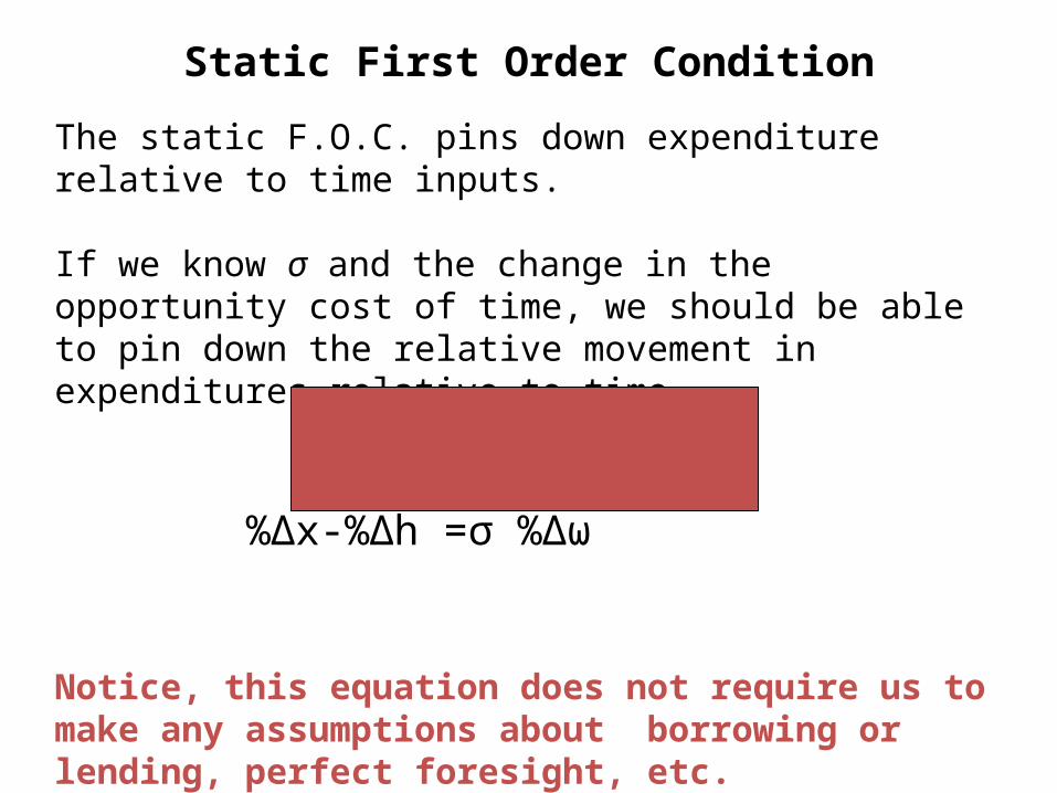
Static First Order Condition

The static F.O.C. pins down expenditure relative to time inputs.

If we know σ and the change in the opportunity cost of time, we should be able to pin down the relative movement in expenditures relative to time.

%Δx-%Δh =σ %Δω

Notice, this equation does not require us to make any assumptions about borrowing or lending, perfect foresight, etc.

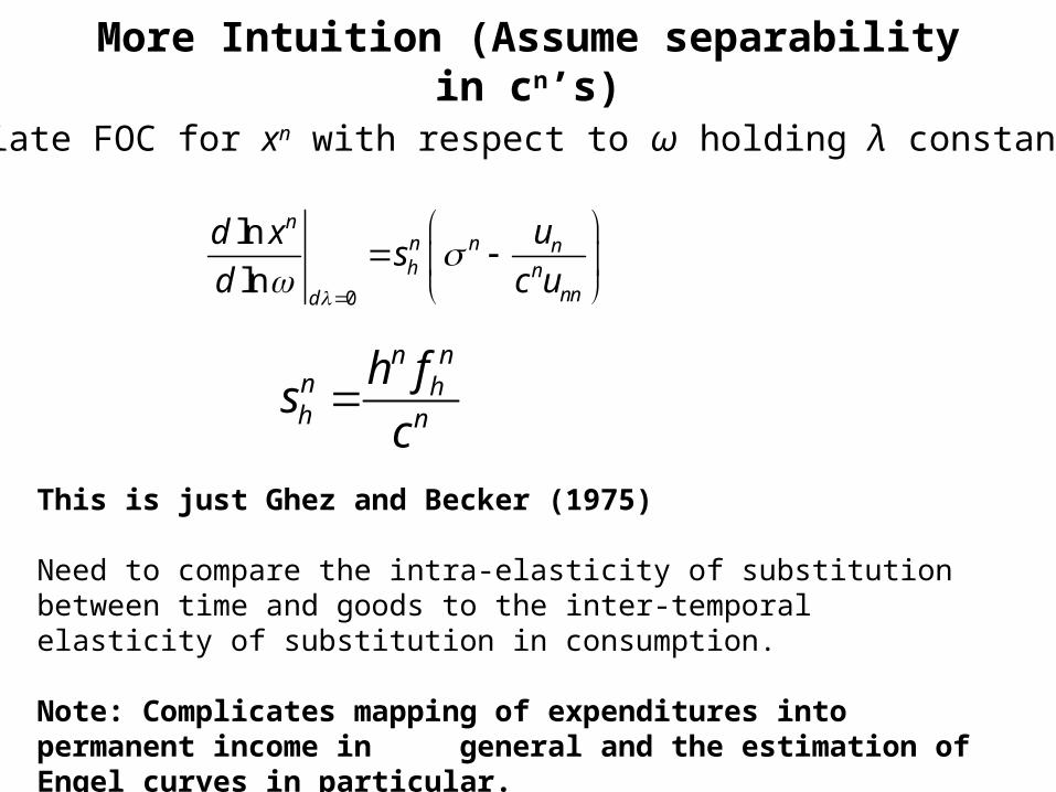
More Intuition (Assume separability in cn’s)

Differentiate FOC for xn with respect to ω holding λ constant. Get:

0

ln

ln

nn n nh n

nnd

ud xs

d c u

n nn hh n

h fs

c

This is just Ghez and Becker (1975)

Need to compare the intra-elasticity of substitution between time and goods to the inter-temporal elasticity of substitution in consumption.

Note: Complicates mapping of expenditures into permanent income in general and the estimation of Engel curves in particular.

Implications

• For given resources (λ):

– As the price of time increases, consumers substitute market goods for time (xn increases) – depends on σn

– As the price of time increases, consumers substitute to periods in which consumption is “cheaper” (xn falls) – depends on the inter-temporal elasticity

• A luxury that is a complement with time should decrease with ω, while a necessity that is a substitute with time should increase with ω.

• Prediction: Entertainment should increase as the price of time decreases, while food should decrease

Different Than Standard Predictions

Differentiate FOC for xn with respect to ω holding λ constant. Get:

Spending should fall the most (with declines in the marginal value of wealth) for goods that have high intertemporal elasticities of substitution.

“Entertainment” spending should decline more with shocks to permanent income than “Food” spending.

0

ln

ln

nn

nnnd

ud c

d c u

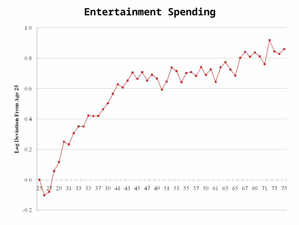
Entertainment Spending

All Non Decreasing Categories

-0.50

0.00

0.50

1.00

1.50

2.00

2.50

3.00

25 30 35 40 45 50 55 60 65 70 75

Log

Dev

iati

on fr

om A

ge 2

5

Entertainment Utilities Housing Services Other ND Domestic Svcs

Decreasing Categories

-1.20

-1.00

-0.80

-0.60

-0.40

-0.20

0.00

0.20

0.40

25 30 35 40 45 50 55 60 65 70 75

Log

Dev

iati

on f

rom

Age

25

Age

Clothing Transportation Food at Home Food Away

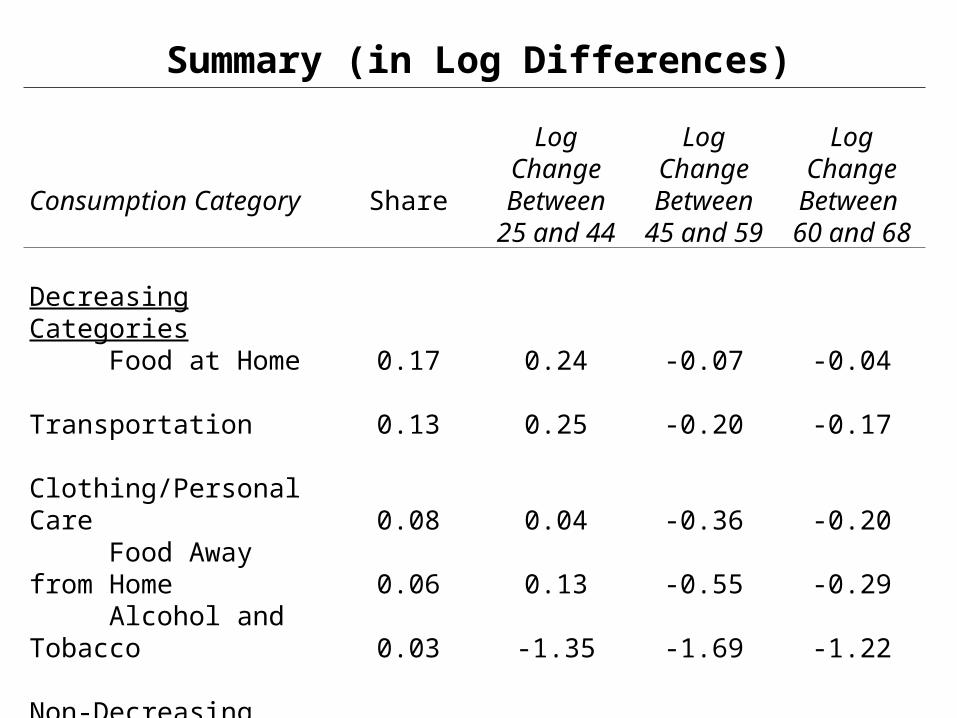
Summary (in Log Differences)

Consumption Category Share

Log Change Between

25 and 44

Log Change Between

45 and 59

Log Change Between 60 and 68

Decreasing Categories Food at Home 0.17 0.24 -0.07 -0.04 Transportation 0.13 0.25 -0.20 -0.17 Clothing/Personal Care 0.08 0.04 -0.36 -0.20 Food Away from Home 0.06 0.13 -0.55 -0.29 Alcohol and Tobacco 0.03 -1.35 -1.69 -1.22

Non-Decreasing Categories Housing Services 0.33 0.73 0.23 0.14 Utilities 0.11 0.72 0.28 0.11 Entertainment 0.04 0.80 0.07 0.17 Other Non-Durable 0.03 1.44 0.16 0.17 Domestic Services 0.02 1.52 0.30 0.32

Food, Transportation and Clothing

• Food is amenable to “Beckerian” home production (see Aguiar and Hurst 2005, 2007)

No evidence of any decline in food intake over the lifecycle despite declining food expenditures.

As opportunity cost of time declines later in life, households substitute towards home production of food (including more intense shopping for bargains).

Data (and calibrated model) actual show food intake increases over the back half of the lifecycle

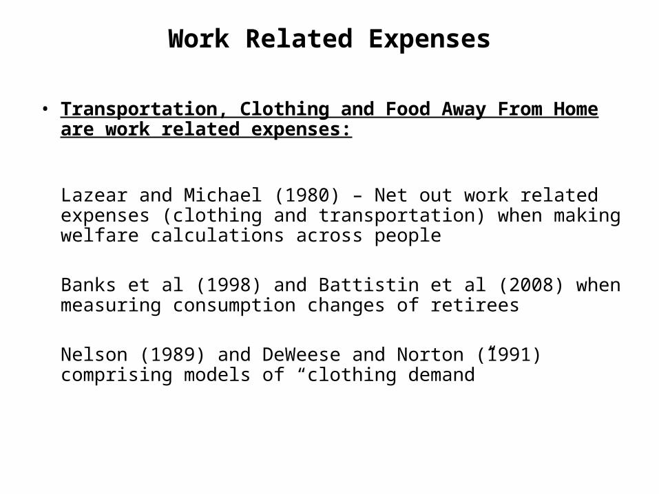
Work Related Expenses

• Transportation, Clothing and Food Away From Home are work related expenses:

Lazear and Michael (1980) – Net out work related expenses (clothing and transportation) when making welfare calculations across people

Banks et al (1998) and Battistin et al (2008) when measuring consumption changes of retirees

Nelson (1989) and DeWeese and Norton (1991) comprising models of “clothing demand”

Level of Work Hours Over the Lifecycle

New Facts About Food, Clothing, and Transport

• Look at food away patterns at different types of establishments

• Look at changes in different amounts of transportation patterns using time use data

• Estimate “simple” demand systems and control directly for work status

Propensity To Eat Away At Home

Propensity To Eat Away At Home

Propensity To Eat Away At Home

Travel Times and Employment Status

Travel Times and Employment Status

Travel Times and Employment Status

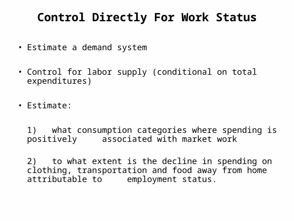
Control Directly For Work Status

• Estimate a demand system

• Control for labor supply (conditional on total expenditures)

• Estimate:

1) what consumption categories where spending is positively associated with market work

2) to what extent is the decline in spending on clothing, transportation and food away from home attributable to employment status.

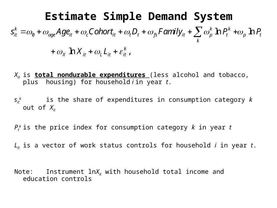
Estimate Simple Demand System

Xit is total nondurable expenditures (less alcohol and tobacco, plus housing) for household i in year t.

sitk is the share of expenditures in consumption category k out of Xit

Ptk is the price index for consumption category k in year t

Lit is a vector of work status controls for household i in year t.

Note: Instrument lnXit with household total income and education controls

0 ln ln

ln ,

k k kit age it c it t t fs it p t p t

k

kX it L it it

s Age Cohort D Family P P

X L

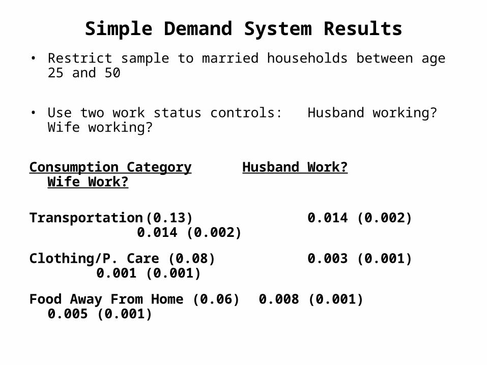
1. Simple Demand System Results

• Restrict sample to married households between age 25 and 50

• Use two work status controls: Husband working? Wife working?

Simple Demand System Results

• Restrict sample to married households between age 25 and 50

• Use two work status controls: Husband working? Wife working?

Consumption Category Husband Work? Wife Work?

Transportation (0.13) 0.014 (0.002) 0.014 (0.002)

Clothing/P. Care (0.08) 0.003 (0.001) 0.001 (0.001)

Food Away From Home (0.06) 0.008 (0.001) 0.005 (0.001)

Simple Demand System Results

• Restrict sample to married households between age 25 and 50

• Use two work status controls: Husband working? Wife working?

Consumption Category Husband Work? Wife Work?

Transportation (0.13) 0.014 (0.002) 0.014 (0.002)

Clothing/P. Care (0.08) 0.003 (0.001) 0.001 (0.001)

Food Away From Home (0.06) 0.008 (0.001) 0.005 (0.001)

Housing Services (0.34) -0.009 (0.003) -0.012 (0.002)

Utilities (0.12) -0.005 (0.001) -0.003 (0.001)

Food At Home (0.18) -0.016 (0.002) -0.013 (0.001)

Entertainment (0.04) 0.000 (0.001) 0.000 (0.001)

2. Adding Work Controls To the Lifecycle Profile

• Married Sample, 25 – 75

• Work Status Controls:7 Dummies for Husband Weeks Worked7 Dummies for Wife Weeks Worked9 Dummies for Hours per week Husband Worked9 Dummies for Hours per week Wife Worked

• Three Categories:Food (food at home and food away)Work Related Expenses (transportation and clothing)Core Non Durables (everything else)

• Ask: “How do work status controls effect lifecycle profiles?”

Demand Estimates, Transportation

-0.045-0.040-0.035-0.030-0.025-0.020-0.015-0.010-0.0050.0000.0050.010

25 30 35 40 45 50 55 60 65 70 75

Sh

are

of E

xpen

dit

ure

:

Dif

fere

nce

fro

m A

ge 2

5

Age

Demand Estimates, Food Away

-0.020

-0.015

-0.010

-0.005

0.000

0.005

25 30 35 40 45 50 55 60 65 70 75

Sh

are

of E

xpen

dit

ure

:

Dif

fere

nce

fro

m A

ge 2

5

Age

Demand Estimates, Clothing

-0.040-0.035-0.030-0.025-0.020-0.015-0.010-0.0050.0000.005

25 30 35 40 45 50 55 60 65 70 75

Shar

e of

Exp

endi

ture

: D

iffe

renc

e fr

om A

ge 2

5

Age

Level of Lifecycle Expenditure

-0.8

-0.6

-0.4

-0.2

0.0

0.2

0.4

0.6

0.8

1.0

1.2

25 30 35 40 45 50 55 60 65 70 75

Log

Dev

iati

on f

rom

Age

25

Work Related Core Nondurables Food at Home

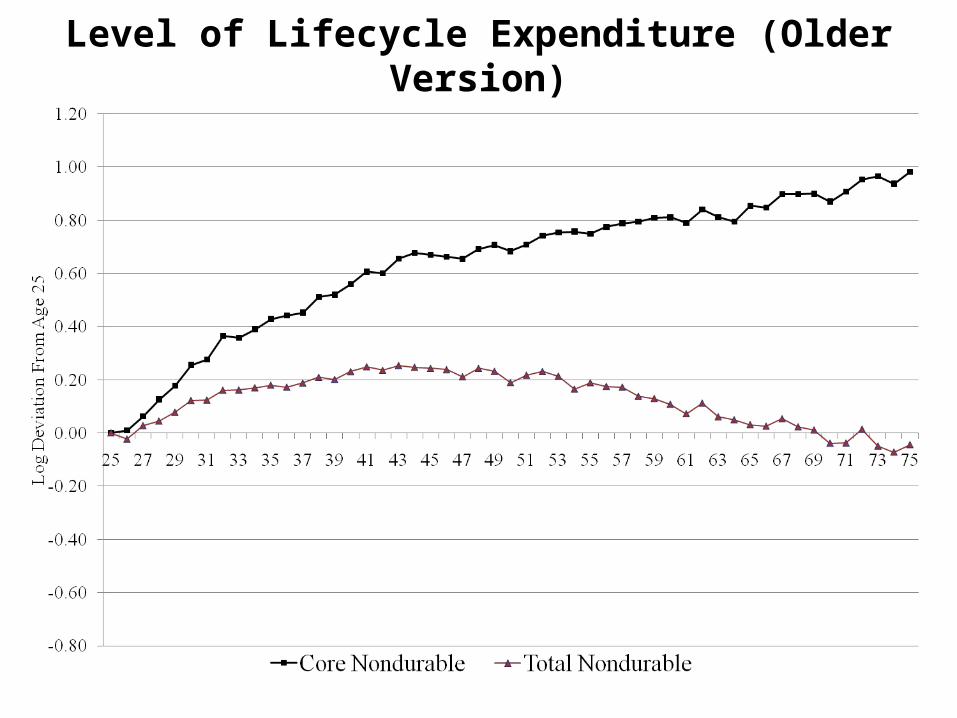
Level of Lifecycle Expenditure (Older Version)

What Does it Mean?

• Aguiar and Hurst (2009)

Write down a model where households maximize utility with three consumption goods (and leisure) with the following constraints:

one good (food) is amenable to home productionone good (transport, clothes) are complements to market workthere is a time budget constraint

Assumptions:

o conditional on work, income process is uncertaino take the lifecycle process of work as exogenouso assume that individual receives no utility for the lifecycle component of work related expenses.

What Does it Mean?

• More on this next week (when we use the same procedure to examine the lifecycle profile of consumption inequality and the time series profile of consumption inequality).

• However – just by looking at the previous figures – households appear to be much more patient than estimated by previous authors!

Some Concluding Thoughts (Again)

• Technically, preferences between “consumption” and leisure are not substitutes.

– Leisure goes up dramatically in retirement (we will show this in a few weeks).

– Consumption (as measured by intake) remains roughly constant (if anything it increases slightly).

• However, “expenditures” and leisure could still be non-separable.

– Non-separability enters through “home production”

• Acknowledging this has implications for: estimating preferences, explaining business cycle frequencies of consumption, examining time series implications of inequality, and estimating the income process from consumption data.