Michigan and Ohio K-12 Educational Financing …conlinmi/finalconlinthompson.pdf · Michigan and Ohio K-12 Educational Financing Systems: Equality and Efficiency ... amount of state

1

Michigan and Ohio K-12 Educational Financing Systems:

Equality and Efficiency

Michael Conlin* Michigan State University Marshall‐AdamsHall

486WCircleDr.Rm110EastLansing,[email protected]

517‐355‐0285(Office)517‐432‐1068(fax)

Paul N. Thompson

Michigan State University Marshall‐AdamsHall

486WCircleDr.Rm110EastLansing,[email protected]‐355‐7583(Office)517‐432‐1068(fax)

February 2014

* corresponding author

(JEL Classifications: I24, I280, H710)

Acknowledgments: We thank Leslie Papke for valuable advice. We also thank seminar participants at the Lincoln Institute’s October 2013 conference entitled The Property Tax and Financing of K-12 Education, Michigan State University and the Michigan/Michigan State/Western Ontario Labor Day Conference.

2

Abstract

We consider issues of equality and efficiency in two different school funding systems - a state-level system in Michigan and a foundation system in Ohio. Unlike Ohio, the Michigan system restricts districts from generating property or income tax revenue to fund operating expenditures. In both states, districts fund capital expenditures with local tax revenue. Our results indicate that although average revenue and expenditures per pupil in Michigan and Ohio are almost identical, the distributions of the various revenue sources are quite different. Ohio’s funding system has greater equality in terms of total revenue, largely due to Ohio redistributing state funds to the least wealthy districts while Michigan does not. We find that relatively wealthy Michigan districts spend more on capital expenditures while relatively wealthy Ohio districts spend more on labor and materials. This suggests that constraints on raising local revenue to fund operating expenditures in Michigan could create efficiency issues.

3

I. Introduction

In the current financial climate, reductions in property values and poor state fiscal conditions

have led to budgetary issues for local school districts. How districts choose to respond to these

financial pressures depends on the level of state funding and the different types of local taxes

available to school districts. Districts that receive greater state aid will likely be sensitive to

reductions in state budgets, while districts with greater ability to raise revenue locally may

respond to declining state and local economic conditions through the use of voter approved tax

referenda.1 In addition, districts with the ability to tax income may be better able to respond to

declines in property values by switching their tax mix away from property taxation and towards

greater income taxation. Districts that are restricted from collecting local tax revenue for

operating expenditures may use other avenues, such as expenditure cuts and alternative revenue

sources, to alleviate these financial pressures.2 The feasibility of these other avenues will clearly

depend on the wealth of the districts. Preventing districts from generating local tax revenue for

operating expenditures, but not imposing these restrictions on capital expenditures, may also

affect how districts allocate resources across capital and operating (i.e., labor and materials)

expenditures. Therefore, in addition to equality considerations, these restrictions may also have

efficiency implications.

Much of the previous literature on equality in school funding has focused on law changes,

usually as a result of court rulings. As expected, these studies largely find that inequality in

1Dye and Reschovsky (2008) find that local school districts increased property taxes by 37 cents for every dollar lost in state aid. 2 Reschovsky (2004) argues that funding constraints limit the ability of districts to respond to reductions in state aid and reductions in taxable values, exacerbating the financial problems facing these districts. Evidence from California suggests that these types of restrictions are often circumvented by increases in non-restricted revenue and non-traditional funding sources, such as private donations (Brunner and Sonstalie, 2003; Brunner and Imazeki, 2005; Hoane, 2004).

4

revenues and expenditures is reduced as a result of these court-mandated reforms.3 Instead of

focusing on law changes, we consider how different funding systems impact inequality.4 We

assess the degree of inequality in per pupil revenue and expenditures across districts under two

distinct funding systems -- a state-level system (i.e. minimal local control) in Michigan and a

foundation system (i.e. greater local control) in Ohio.5 Both states use different mechanisms to

adjust for inequality resulting from differences in tax base size. Michigan keeps state aid roughly

the same for all districts regardless of tax base size, but attempts to minimize inequality in

revenue by restricting the collection of local revenue to fund operating expenditures for general

education students. The Michigan system does allow residents to vote for property tax millages

that finance capital projects and expenditures on special and vocational education. Ohio allows

districts to raise unrestricted funds for operating expenditures through local property and income

taxes, but accounts for the large inequality this creates by giving a disproportionately large

amount of state aid to districts with the smallest tax bases. This paper assesses whether the

degree of inequality in revenues and expenditures varies across these two states. We also

examine whether the allocation of resources between capital and operating expenditures varies

across the different funding systems.

Section II provides an overview of the Michigan and Ohio K-12 education financing systems.

Section III first describes the data and contains descriptive statistics on tax rates, taxable values

and district demographics. It then contains a comparison across different revenue sources and

3Murray, Evans, and Schwab (1998) and Corcoran et al. (2004) find that inequality wasreduced by 19 to 34 percent follow these reforms, relative to non-reform states. Also, see Springer, Liu, and Guthrie (2009), Roy (2011), and Berry (2007). For a larger review of the state role on equity and adequacy, see Corcoran and Evans chapter in the Handbook of Research in Education Finance and Policy (2008).4For an overview of different state aid formulas, see Loeb (2001), Hoxby (2001), Fernandez and Rogerson (2003), and Yinger (2004). 5Theoretical work by Fernandez and Rogerson (2003) suggests that the foundation system dominates the state-level system in terms of total welfare.

5

whether this varies across districts based on property values per pupil. Finally, Section III

compares expenditures across districts and discusses whether the composition of these

expenditures varies across the states. Section IV concludes.

II. Institutional Details

The Michigan and Ohio K-12 education financing systems are quite complicated and differ

along several significant dimensions. Perhaps the most important difference is the restriction on

local tax revenue collection for operating expenditures in Michigan. This section provides an

overview of the Michigan and Ohio funding systems and discusses the differences and

similarities of the two systems.

2.1 Michigan K-12 Finance

In response to high property taxes and an unequal distribution of school funding across

districts, the Michigan K-12 finance system changed dramatically with the implementation of

Proposal A in 1996. Proposal A changed the power equalization finance system to a state level

system and reduced the funding obtained from local property taxes while increasing the funding

from state income and sales taxes. School districts with a millage rate over 18 in fiscal year 1993

had their millage rate reduced to 18 and the new law stipulated that districts only impose this

millage on non-homestead properties.6,7 In addition to this non-homestead millage, the state

allowed 32 of the highest-spending school districts to levy a “hold harmless” millage. The state

also imposed a state level property tax of six mills along with increases in the sales, tobacco

product, and real estate transfer taxes. Proceeds from these taxes are deposited in the Michigan

6 Homestead properties are primary resident homes while non-homestead properties are mainly businesses and rental properties. 7 Only 13 of the 552 school districts imposed a millage of less than 18 in fiscal year 1993. For these districts, the non-homestead millage is capped at the 1993 rate.

6

School Aid Fund and distributed to the school districts through a per-pupil grant. This grant

varies depending on which school district the student resides, but does not depend on the amount

of local property taxes collected. The amount of the per-pupil grant is the difference between the

amount of local revenue that would be collected if the non-homestead millage is at its cap,

usually 18 mills, and the amount required to achieve the school district’s per-pupil grant

allocation. The funds from the grant are deposited into the school district’s general fund to pay

for labor, material, utilities and maintenance costs. Along with property tax millages to finance

capital projects, local school districts can propose a “sinking fund” property tax millage, the

revenues of which fund certain capital expenditures and repairs.8 Local school districts can also

generate funds using voter-approved referenda for a recreational millage, which provide revenue

for the operation of public recreation facilities and playgrounds.

Each of the 552 local school districts in Michigan belongs to one of 57 intermediate school

districts (ISDs) that provide special and vocational education. Funding of ISDs did not

appreciably change due to Proposal A and a significant portion of ISD funding comes from local

property taxes. The variation across ISDs in regards to property tax revenue results in vastly

different services being offered across the ISDs. Some of these services are offered directly by

the ISD, while others are provided by the local school districts using ISD funds. An ISD can levy

three types of property tax millage: operational, special education and vocational education.

Voters must pass a referendum to change any of these millage rates and there are caps associated

with all three tax millages.9 The amount of revenue that is passed on to the local school districts

8 The maximum sinking fund millage is five mills for twenty years. 9 The operating millage rate cannot exceed 1.5 times the number of mills allocated to the ISD in 1993. The special education millage rate cannot exceed 1.75 times the number of mills allocated to the ISD in 1993. The vocational education millage rate is capped at 1 mill for those ISDs that did not levy this tax in 1993 and is capped at 1.5 times the number of mills allocated to the ISD in 1993 for all other ISDs.

7

varies across ISDs.10 Along with these property taxes, voters may approve referenda for

enhancement millages, the proceeds of which are distributed by the ISD to their local school

districts on a per student basis.11

There have been a few post-2002 changes to the Michigan K-12 education financing system.

One noteworthy change occurred in 2008, when industrial personal property was exempted from

both the non-homestead property tax millage (which is usually 18 mills) and the state level

property tax of six mills. During the same time commercial personal property was exempted

from 12 of the 18 non-homestead property tax mills.12 Since 2002, the number of students

attending charter schools has increased substantially in Michigan. Charter schools are operated

as nonprofit corporations that, like public schools, are provided with the state per pupil

foundation allowance but are prohibited from levying taxes which results in capital expenses

being paid for by the foundation allowance or independent contributions.

2.2 Ohio K-12 Finance

The 613 public school districts and 49 joint vocational school districts13 in Ohio are primarily

funded through state aid and local property or income taxation. The role of the state in financing

education is to ensure that each district receives the necessary funds to provide an “adequate”

level of educational services to the students of the district. To do this, the state first determines

the amount of per pupil expenditures that are necessary to achieve this adequate education

10The majority of ISDs base the distribution of the revenue from the special education millage on the difference between the special education costs of the district and the amount received in state aid. Other ISDs base the distribution on average cost measures and the number of special education students. 11 The maximum enhancement millage is three mills for twenty years.12 Personal property is tangible assets of a business such as computers, machinery and equipment. Real property refers to land and buildings.13 These vocational schools span one or more counties within the state. They provide vocational training to students from public school districts within the counties the vocational school operates. High school students from these public school districts can opt to pursue this vocational training in place of a traditional public high school education, if accepted into the vocational program.

8

level.14 School districts are required to raise at least 20 mills of property tax revenue in order to

cover some (or all) of this adequacy amount. Currently, the state calculates the local share of the

adequacy amount by assuming school districts levy 23 mills of property taxes.15 After netting out

this local “charge-off”, the state provides districts with the remaining revenue needed to achieve

the adequacy amount.

Ohio school districts also have the option to supplement state aid through additional property

and income taxation, subject to voter approval. Districts are able to tax both real and tangible

personal property.16 Similar to Michigan, districts can issue debt through bonds for capital

projects and improvements to classroom facilities. In addition to debt issuances, permanent

improvement property tax levies fund short-term, at most five year, capital improvements. In

contrast to Michigan, Ohio districts also have the option to propose additional taxes financing

operating expenditures. Revenue for operating expenditures is generated through either current

expense millages or emergency operating levies. These current expense taxes can either be

property or income taxes that raise revenue over a period of five or more years.17 Emergency

operating taxes collect a district-specified amount of revenue for a period of, at most, five years.

In addition to taxes approved by voters, each district is allocated a set amount of property tax

millage that is levied without voter approval. Districts primarily allocate the revenue from this

“inside millage” towards either current expenses or permanent improvements.

14 For documentation on the adequacy formula, see the Ohio Legislative Service Commission “School Funding Complete Resource.” (http://www.lsc.state.oh.us/schoolfunding/edufeb2011.pdf) 15 There are a few districts that impose less than 23 mills. The state supplements these districts with enough funds to meet the revenue that would have been received had the district levied 23 mills. This additional state supplement is called gap aid. 16 There are two classes of real property in Ohio: class I includes all real residential and agricultural property and class II includes all real commercial, industrial, mineral, and railroad property.17 Prior to 2006, Ohio school districts could levy income taxes on the traditional income tax base (adjusted gross income net personal and dependent exemptions). After 2006, districts were given the option of only taxing the earned income of residents. This earned income is not subject to personal and dependent exemptions.

9

There have been a few significant policy changes since 2002 that have changed the way

schools are funded. In 2010, Ohio adopted an evidence-based funding formula that determined

the adequacy amount based on the number and type of staff needed to provide a basic level of

education. This funding formula also changed how the local share of funding is calculated. Prior

to 2010, the local “charge-off” was calculated using recognized valuation.18 Starting in 2010, the

local “charge-off” for districts at the 20-mill floor was calculated using total valuation, while the

charge-off of all other districts continued to be calculated using recognized valuation. Beginning

in 2006, Ohio gradually phased out taxation on business tangible personal property, with the

state providing districts with funds to offset the loss in revenue resulting from this phase out.

2.3 Similarities Between Ohio and Michigan Financing Systems

There are several similarities between the two school funding systems. Michigan and Ohio

both have school choice programs, which allow students to attend a school district even if they

do not reside in that district. The state provides the attending district with additional funds to

educate these students. For school districts that have capacity and elect to enroll students residing

outside the district boundaries, Michigan requires the district to hold a lottery to determine which

students are able to attend – with preference given to students with siblings who are already

school of choice students in the district. Unlike Michigan, school districts in Ohio do not hold

lotteries to determine which students are able to attend via open enrollment. Instead, the school

superintendent determines which students are allowed to enroll in the school district when the

18 Recognized valuation spreads out the inflationary increase in real property from reappraisal over three years to prevent the state share of funding to fluctuate greatly from one year to the next. Thus, the recognized valuation of a district in the year of reappraisal is the total valuation – (2/3)*Inflationary Increase. A year after reappraisal, recognized valuation becomes the total valuation – (1/3)*Inflationary Increase. Two years after reappraisal, recognized valuation is equal to total valuation. Also, since the school fiscal year runs from July to June and the tax year runs from January to December, valuation from two years prior is used in the calculation of the local charge-off. For example, valuation from 2008 is used in the calculation for the 2009-2010 school year.

10

number of open enrollment applications exceeds the number of slots available. School districts in

Ohio also have the option to limit what students are eligible to enroll in the district through open

enrollment.19

Another similarity is that both states have legislation that restricts the growth of local

property taxes. The 1978 Headlee Amendment in Michigan requires that property tax rates be

decreased (i.e. “rolled back”) if the growth in assessed values, excluding new construction and

improvements, exceeds the growth in inflation. County, municipality, intermediate school district

and school district property tax rates are “rolled back” so that the same amount of property taxes,

in real terms, are collected from the old base.20 For parcels that do not transfer ownership,

Proposal A also restricts the growth of individual parcel property assessments to the lesser of the

inflation rate and five percent. For parcels that do transfer ownership, the taxable values are

assessed at 50 percent of the true cash value. Ownership transfers usually result in a significant

increase in the amount of property tax paid on these properties. Residents can “override” these

Headlee rollbacks by voting on referenda that returns the tax rate back to its prior level or by

voting on renewal specifying the prior tax rates.21

In Ohio, property taxes for current expenses (provided total current expense millage is

greater than 20 mills), classroom facilities and permanent improvements are subject to property

tax rollbacks. Bonds, emergency operating levies, and all inside millage are exempt from these

property tax rollbacks. All real property (both class I and class II) is assessed at 35 percent of

true value. Tangible personal property is assessed at a rate between 23 percent and 100 percent

19 Currently, 431 Ohio school districts allow any student from the state to apply for open enrollment. Of the remaining districts, 62 only accept students from adjacent districts and 120 have no open enrollment policy in place. 20 Millage used to retire debt, along with the 6 mill state level property tax, are not subject to these Headlee roll backs. 21 Many districts pass referenda stipulating a “maximum” non-homestead property tax millage of over 18. While the districts are restricted to only levy 18 mills, passing this type of referenda allows a district facing a Headlee rollback to maintain an 18 millage rate without voting on another referendum.

11

of true value. Similar to Michigan, these property tax rollbacks require that class I and class II

property tax rates be reduced in proportion to the increase in assessed values. Tangible personal

property is exempt from these rollbacks. Since changes in assessed valuation of class I and class

II property differ, the rollback factor is different for both classes of real property. Therefore,

often class I and class II real property are taxed at different rates, while tangible personal

property is taxed at the voted millage rate.

III. Data and Descriptive Statistics

3.1 Data

We obtained school district specific variables from the National Center for Education

Statistics (Local Education Agency Finance Survey and Common Core of Data), the Michigan

Department of Education, the Ohio Department of Education, the Michigan Department of

Treasury, and the Ohio Department of Taxation. Detailed information on school district revenues

and expenditures is obtained from the Local Education Agency Finance Survey. These data

consist of annual school district information from 2002 through 2010.22 These data include

information on total revenues, total federal revenues, total state revenues, total local revenues,

and total expenditures. These data also include a measure of total enrollment in the district,

which we supplement with data on the number of general education and special education

students from the Ohio and Michigan Departments of Education. School district demographic

data are obtained from the NCES Common Core of Data and the Small Area Income and Poverty

Estimates. These data include the number of free and reduced priced lunch students, enrollments

22 Year corresponds to the school fiscal year from July 1st to June 30th. Thus, we analyze data from the 2001-2002 school year to the 2009-2010 school year.

12

broken down by race, number of schools in the district, and the number of school-aged children

in poverty.

We also collect annual tax rates and taxable property valuations from the Michigan

Department of Treasury and the Ohio Department of Taxation. The tax information provides all

the taxes levied in each year from 2002 through 2010 and includes information for whether the

tax funds operating or capital expenditures. We then aggregate these tax rates at the district level,

which provides us with a total district tax rate to fund operating expenditures and a total tax rate

to fund capital expenditures. We then multiply these two aggregate tax rates by the total taxable

value in the district for each year, which gives an estimate of the total local property tax revenue

collected to fund operating and capital expenditures. We also obtain a measure of the level of

income taxes collected by Ohio districts for operating expenditures from the Local Education

Agency Finance Survey.

3.2 Descriptive Statistics

Table 1 contains the average school district property tax rates for Michigan and Ohio along

with taxable value information. There are interesting differences to note across the states. While

both the local school districts and the intermediate school districts in Michigan collect property

taxes, the local school districts in Ohio have a much higher overall millage rate from which to

generate unrestricted operating revenue. This is due to the fact that Michigan imposes a dollar for

dollar “tax” on revenue generated from the non-homestead millage and, therefore, this non-

homestead revenue should be and is considered state revenue in our analysis. For Ohio, the local

revenue generated to cover the adequacy amount defined by the state is considered local revenue.

While we do not have district level information on these adequacy amounts, for most Ohio

13

districts, especially the relatively wealthy districts, we expect that the current tax rates more than

cover the adequacy amount and a nominal change in the tax rates will not change the revenue

obtained from the state. Table 1 also indicates that the taxable values, on which these local

property taxes are imposed, are greater for Michigan. Since the average number of students in a

school district is 2,774 for Michigan and 2,870 for Ohio (Table 2), the taxable value difference

between Michigan and Ohio is not the result of Ohio having larger school districts. Taxable

values differ across the two states because Ohio properties are assessed at only 35 percent of true

value compared with a 50 percent assessment rate in Michigan; resulting in the taxable value per

pupil being over twice as large in Michigan.

Table 2 indicates that, along with slightly larger enrollments, Ohio school districts have

slightly greater total expenditures and total revenue on average than Michigan.23 This results in

almost identical total expenditures per student and total revenue per student, on average, for the

two states. Total revenue is slightly greater in Ohio than Michigan because while Ohio districts

average $8.3 million (23.1-14.8) less in state revenue, they average $10.6 million (16.8-6.22)

more in local revenue than Michigan. Local revenue is comprised primarily of local property and

income taxes but there are other sources of local revenue including school lunch receipts, student

activity receipts, student fees and transfers from other school districts.24 Greater local tax

revenue by Ohio districts is expected because the larger overall millage rates more than offset the

lower taxable values. 25,26 This greater local tax revenue collection in Ohio is mainly attributable

23 Using the Consumer Price Index, dollar figures in all tables and figures have been converted into 2010 dollars. 24 Excluding local property and income tax revenue, Ohio districts average $2.7 million annually from other local revenue sources while Michigan districts average $3.0 million annually. This includes revenue from other school districts (primarily payments associated with school choice programs and transfers from the ISDs), which average $1.4 million and $0.4 million annually for Michigan and Ohio districts, respectively. While we include these transfers from other school districts as local revenue, it may be more appropriate to classify some as state revenue. 25 The local taxes collected as reported by the districts in the Local Education Agency Finance Survey are less than the amounts calculated using the millage rates and taxable value information. Part of this difference is attributable to the fact that when we use the millage rates and taxable value information from the Michigan Department of

14

to Ohio’s current expense millage and is not appreciably affected by local income tax revenue,

which averages only $400,000 annually for Ohio school districts.

While Ohio generates more local revenue for operating expenses, Michigan generates

significantly more for capital expenditures. The reason the taxation for capital expenditures

differ so dramatically is in part due to the Ohio School Facilities Commission (OSFC). The

OSFC is a state agency that provided funds for capital expenditures (e.g. school building

construction and renovations) to the school districts. Besides the number of special education

students and number of Title I schools, the averages of the other school district demographic

characteristics are similar across the states.27 While the difference in the number of Title I

schools is surprising, the fewer number of special education students in Michigan local school

districts is partly attributable to the fact that many Michigan special education students attend

schools operated by the intermediate school districts.28

3.2.1 School District Revenue

Figures 1 through 6 present yearly student enrollment and per pupil revenue from different

sources across different quintiles based on average annual taxable property values per pupil. To

compare the inequality in these various revenue sources, separate graphs are provided for

Treasury and the Ohio Department of Taxation, we do not take into account the various tax exemptions received by some property owners nor delinquent payments. 26 It is important to note that the difference in local revenue per pupil would be less if the non-homestead millage in Michigan was considered local revenue or if the local revenue generated by Ohio districts to achieve the adequacy amount was considered state revenue. 27 It should be noted that the number of free and reduced lunch students is not available for Ohio in 2008, but removing this variable from our regressions does very little to change the main conclusions. In addition, the median income by school district is available in the 2000 U.S. Census and 5-year estimates are available from the Census for all Ohio, and almost all Michigan school districts from 2005-2009, 2006-2010 and 2007-2011. We construct annual median income by district by interpolating this information. 28 In addition, the structure of special education financing in Ohio provides districts more incentive to classify a student as special education relative to Michigan.

15

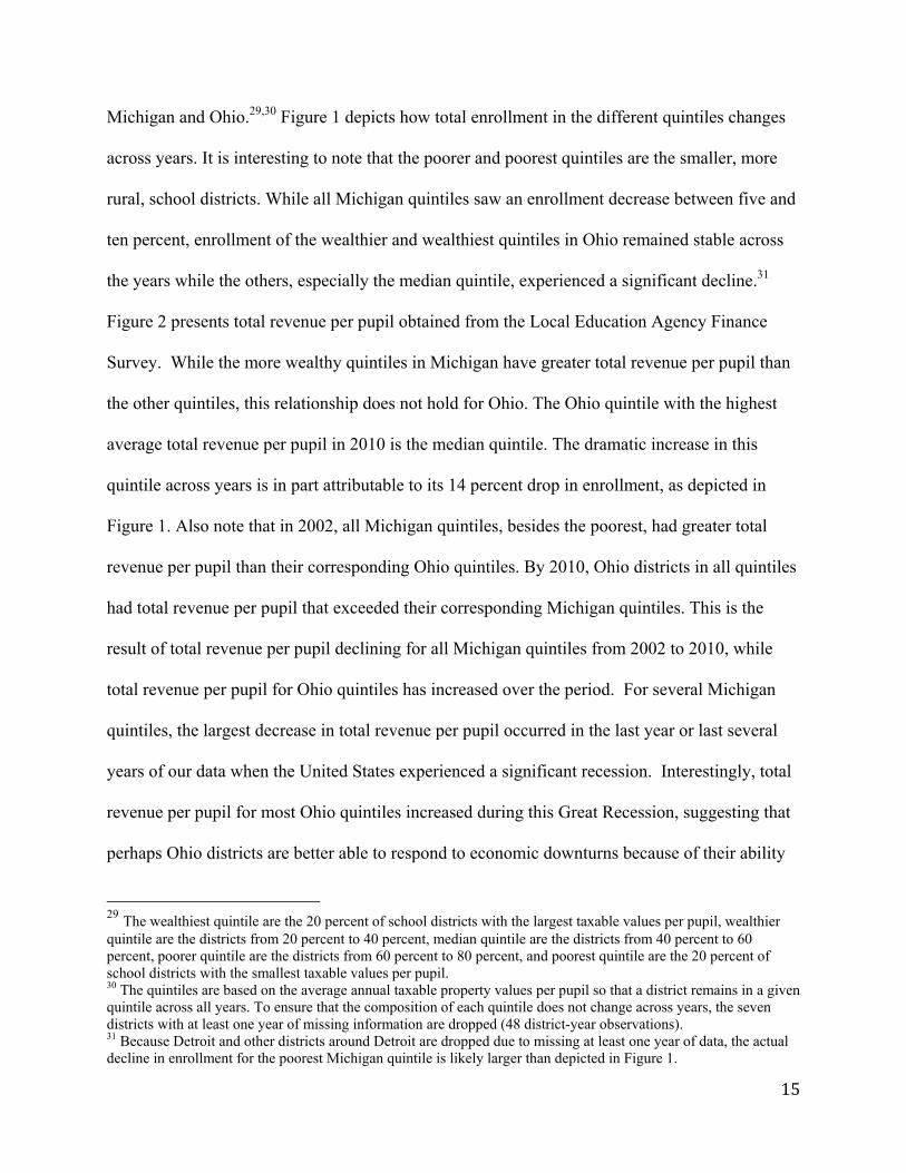
Michigan and Ohio.29,30 Figure 1 depicts how total enrollment in the different quintiles changes

across years. It is interesting to note that the poorer and poorest quintiles are the smaller, more

rural, school districts. While all Michigan quintiles saw an enrollment decrease between five and

ten percent, enrollment of the wealthier and wealthiest quintiles in Ohio remained stable across

the years while the others, especially the median quintile, experienced a significant decline.31

Figure 2 presents total revenue per pupil obtained from the Local Education Agency Finance

Survey. While the more wealthy quintiles in Michigan have greater total revenue per pupil than

the other quintiles, this relationship does not hold for Ohio. The Ohio quintile with the highest

average total revenue per pupil in 2010 is the median quintile. The dramatic increase in this

quintile across years is in part attributable to its 14 percent drop in enrollment, as depicted in

Figure 1. Also note that in 2002, all Michigan quintiles, besides the poorest, had greater total

revenue per pupil than their corresponding Ohio quintiles. By 2010, Ohio districts in all quintiles

had total revenue per pupil that exceeded their corresponding Michigan quintiles. This is the

result of total revenue per pupil declining for all Michigan quintiles from 2002 to 2010, while

total revenue per pupil for Ohio quintiles has increased over the period. For several Michigan

quintiles, the largest decrease in total revenue per pupil occurred in the last year or last several

years of our data when the United States experienced a significant recession. Interestingly, total

revenue per pupil for most Ohio quintiles increased during this Great Recession, suggesting that

perhaps Ohio districts are better able to respond to economic downturns because of their ability

29 The wealthiest quintile are the 20 percent of school districts with the largest taxable values per pupil, wealthier quintile are the districts from 20 percent to 40 percent, median quintile are the districts from 40 percent to 60 percent, poorer quintile are the districts from 60 percent to 80 percent, and poorest quintile are the 20 percent of school districts with the smallest taxable values per pupil. 30 The quintiles are based on the average annual taxable property values per pupil so that a district remains in a given quintile across all years. To ensure that the composition of each quintile does not change across years, the seven districts with at least one year of missing information are dropped (48 district-year observations). 31 Because Detroit and other districts around Detroit are dropped due to missing at least one year of data, the actual decline in enrollment for the poorest Michigan quintile is likely larger than depicted in Figure 1.

16

to generate local revenue for operating expenditures. Thus, the structure of the state school

financing system may greatly influence how economic downturns impact school districts.

As demonstrated in panel (a) of Figure 3, Michigan’s slight decrease in total revenue per

pupil is primarily attributable to a decrease in state revenue. Given that Michigan restricts how

much revenue can be raised locally to fund operating expenditures, it is not unexpected that

Michigan districts usually receive more in state revenue per pupil than comparable Ohio districts.

Interestingly, Michigan distributes state revenue relatively evenly across school districts, but

districts in the wealthiest quintile receive nearly $600 more in state revenue per pupil than

districts in the other quintiles. This distribution of state aid, which is provided irrespective of

district wealth, is consistent with what would be expected given the framework of the Michigan

funding laws, which targets inequality by restricting collection of local property taxes. In

contrast, Ohio attempts to address inequality by allocating significantly more state revenue to

less wealthy districts. Districts in the wealthiest quintile in Ohio receive between $3,000 and

$5,800 less state revenue per pupil than districts in the poorest quintile, but this difference has

decreased across years.

Unlike Ohio, which addresses inequality through disproportionate state aid to the poorest

districts, Michigan addresses inequality by placing restrictions on the use of local property taxes

for operating expenditures. These restrictions explain the large differences in local revenue we

observe in Figure 4 between Ohio and Michigan districts in all taxable value quintiles. Michigan

districts obtain approximately two and a half times less local revenue than similar districts in

Ohio. Due to unrestricted property and income taxation at the local level in Ohio, the gap in local

revenue between the richest and poorest districts is much larger in Ohio than in Michigan. While

the wealthiest Michigan school districts raise approximately $2,000 per pupil more in local

17

revenue than the poorest districts, the wealthiest districts in Ohio raise $5,000 more per pupil

than the poorest districts. This disparity between the top and bottom is so large in Ohio that even

though the state gives disproportionately more state revenue to the relatively poor districts it is

not enough to offset this $5,000 per pupil gap.

In addition to the disparity in total local revenue, the restrictions placed on taxes for

operating expenditures in Michigan may result in different mixes of taxes for capital and

operating expenditures across the two states. Figure 5 focuses strictly on local operating tax

revenue, which is generated exclusively through property taxes in Michigan, while Ohio districts

generate local operating revenue through property and income taxes. The minimal local property

tax revenue collected by Michigan districts for operating expenditures is obtained primarily from

the hold harmless millage of wealthy districts and the special education millage of the

intermediate school districts. In contrast to Michigan, a significant portion of local revenue in

Ohio is generated from local taxes and almost all is unrestricted, as state revenue is often used

towards funding special education. As expected based on Figure 4, the amount of local operating

tax revenue generated is greater in the relatively wealthy districts and significantly greater in the

wealthiest districts. In Ohio, a relatively small fraction of local operating revenue is from

income taxes but use of these taxes has increased since 2006 -- especially in poorer, agricultural

districts that have low taxable value bases, but relatively higher taxable income bases.32

As state revenue has decreased and local revenue for operating expenditures has largely

remained constant from 2002 to 2010, property tax revenue for capital expenditures has

increased in Michigan. As depicted in Figure 6, the Michigan quintiles increased property tax

revenue for capital expenditures by between $200 and $300 per pupil, with the largest increase

32 As found in Spry (2005) and Hall and Ross (2010), a majority of districts using these income taxes are districts in rural areas. Ross and Nguyen-Hoang (2013) show that Ohio districts use the income tax as a supplement to property taxation.

18

occurring in the wealthiest quintile. Ohio districts in all quintiles collect less tax revenue for

capital expenditures than districts in the corresponding Michigan quintiles. For the median,

poorer, and poorest quintiles, this difference is partly attributable to the Ohio School Facilities

Commission (OSFC), which designated $7 billion for capital expenditures to, primarily, the

relatively poor school districts between 2002 and 2010.33 The OSFC made these capital funds

available to the least wealthy districts first by ranking the districts based on a weighted average

of taxable value per pupil and median income.34 This capital expenditure subsidy from the OSFC

is likely to have crowded out some capital expenditures by the school districts. Interestingly, the

wealthier and wealthiest quintiles in Ohio, mainly comprised of school districts that did not have

access to these OSFC funds, also obtain significantly less tax revenue for capital expenditures

than comparably wealthy Michigan school districts. Perhaps these wealthy Ohio districts

preferred to have local tax revenue fund operating expenditures rather than capital expenditures.

Because of the constraints Proposal A places on raising local operating revenue, the wealthy

Michigan districts do not have this choice.

Although the above figures give some sense of the inequality of revenue in both states, these

figures do not account for differences in district size and demographics that may contribute to

33 The decision to use a significant portion of the tobacco settlement funds to subsidize school capital investments was, in part, a response to a General Accounting Office report entitled “School Facilities: Profiles of School Condition by State.” The 1996 report summarized results from a national survey of school buildings and concluded that the physical condition of school buildings in Ohio was worse than the school building condition in, if not all, almost all other states. For example, the report indicates that 61 percent of the 3,600 Ohio schools surveyed indicate at least one on-site building in inadequate condition compared to only 34 percent for the 3,325 Michigan schools surveyed. 34 The OSFC began offering funds to the most needy school districts in 1997 and by 2010 funds had worked up to the 450th spot in the rankings. The state has contributed a certain percentage of the capital funds and this percentage depends on the district rankings with poorer districts having lower rankings receiving a greater percentage. For most districts, the state’s percent contribution is one minus the ranking list percentile. For example, a district ranked 61 out of the 613 school districts would be at the tenth percentile and the state contribution would be 90 percent of the total project cost. Most districts raise their share by passing a referendum that generates property taxes so that the district can sell bonds. A few districts use existing property taxes, cash on hand and voluntary contributions to raise the local share. In recent years especially, many districts chose not to pursue the available funding or were unable to pass referenda to fund the district’s portion of the costs.

19

differences in revenue across the two states. To better account for these other factors we estimate

the following regression equation:

ln(yst) = β0 ln(Taxable Valuest) + Xst β+ λs + θt + εst

where ln(yst) is the natural log of either total revenue, state revenue, or local revenue of district s

in year t; ln(Taxable Valuest) is the total taxable value for the district in year t; Xst is a vector of

school district demographics that includes median income, total and special education enrollment

counts, the number of white students, the number of students eligible for free/reduced priced

lunch, the total number of schools and Title I schools, total district population and total school-

aged population in poverty; λs is a vector of school district fixed effects; θt is a vector of year

fixed effects; and εst is an idiosyncratic error term. Tables 3 and 4 contain estimates when school

district fixed effects are not and are included in the specification, respectively.

The estimates from the specification without fixed effects uses primarily across school

district variation to identify the relationship between taxable value and revenue. These estimates

in Table 3 suggest that a ten percent increase in total taxable value is associated with

approximately a 1.3 percent increase in total revenue for both states, while a ten percent increase

in median income is associated with a 2.12 percent increase in total revenue for Michigan and a

negligible change for Ohio. When median income is not included as a covariate, the coefficient

on taxable value when total revenue is the dependent variable increases to 0.146 for Michigan

and to 0.139 for Ohio. As expected based on the graphs in Figure 3, the coefficient estimates

associated with taxable value indicate that state revenue is larger in Michigan districts with

greater taxable values. In Ohio, however, state revenue is significantly less in high taxable value

school districts compared to low taxable value districts, since the state funding laws give these

low taxable value districts disproportionately more state aid. In terms of local revenue, the

20

coefficient estimates indicate that low taxable value districts obtain less in local revenue than

high taxable value districts and this difference is greater in Ohio. The results in Table 3, along

with the greater variance in taxable value and median income for Michigan (see Tables 1 and 2),

suggest that there is greater inequality in Michigan than in Ohio.

The estimates from the fixed effects specifications in Table 4 use within-school district,

across-year variation to identify the relationship between changes in taxable value and changes

in revenue. These estimates indicate that an increase in taxable value is associated with a

significant increase in state, local and total revenues for Michigan school districts. For Ohio

school districts, an increase in taxable value is associated with an increase in local revenue, a

decrease in state revenue, and a slight increase in total revenue. Table 4 also suggests that

changes in median income are associated with relatively small increases in revenue for Michigan

school districts and a negligible change in revenue for Ohio districts.35

The graphs in Figures 2 and 3 suggest that total and state revenues decreased for Michigan

and increased for Ohio school districts during the Great Recession. It is also interesting to

consider how this recession affected taxable values, inequality and the relationship between

taxable value and revenue. Due in part to differences in assessment procedures, Ohio’s assessed

values started to decrease in 2007 (affecting school district’s 2007-8 taxable values) while

Michigan did not experience this decline in taxable values until the 2009-10 school year (denoted

as year 2010). The taxable value per pupil decreased less than taxable values in both states

because of the decline in the number of students. However, the variance of the taxable value per

pupil in both states was much larger after 2007 compared to the prior years. In addition, based on

the estimates in Table 5, the relationship between total taxable value and revenue does appear to

35 Because median income is not available annually by district (requiring us to interpolate when constructing these annual measures - see footnote 27), the coefficient estimates pertaining to median income should be viewed with caution when using within-district, across-year variation for identification.

21

change slightly as the result of the Great Recession. Table 5 estimates similar specifications as in

Tables 3 and 4 except an interaction term, ln(Total Taxable Value) * Great Recession indicator,

is included as a covariate to allow for the relationship between taxable value and revenue from

2002 to 2007 to differ from this relationship from 2008 to 2010. The coefficient estimates

associated with this interaction term indicate that the positive relationships between taxable value

and total/state revenues are stronger during the Great Recession for Michigan school districts but

not for Ohio school districts. While these positive coefficient estimates are statistically

significant in the Michigan regressions, the magnitudes suggest a relatively small increase in

these positive relationships during the Great Recession.

The results in Tables 3 and 4 suggest that the Ohio funding system leads to more equitable

funding than the Michigan system. Targeting equality through disproportionate state aid to the

poorest districts appears to be more effective at promoting equality than imposing constraints on

what local revenue can be used to fund. A problem with the Michigan system is that even with

constraints that limit how much local revenue can be used for operating expenditures, local

revenue is greater in high taxable value districts and does not offset the fact that state aid is not

targeted to relatively poor districts. These constraints may also hinder the ability of Michigan

school districts to react to economic downturns, exacerbating this inequality. While wealthy

districts in Michigan may be able to counteract these downturns with funding from other local

sources, the relatively poor districts in Michigan do not get much funding from other sources,

making them the least able to respond to these downturns. The Table 5 results suggest that the

inequality in Michigan may be growing during the Great Recession. Another problem is that

these constraints could lead to inefficiencies in terms of how local school districts allocate

resources between capital, labor and materials.

22

3.2.2 School District Expenditures

Figure 7 demonstrates that the pattern in total expenditures per pupil is quite similar to total

revenue per pupil both in terms of level and across quintiles. As with total revenue per pupil,

total expenditures per pupil on average are similar across the states with expenditures in

Michigan decreasing slightly across years while increasing in Ohio. Also similar to total revenue

per pupil, Michigan’s decrease in total expenditure per pupil was more prevalent during the

Great Recession while Ohio districts experienced an increase during this time period. The main

difference in per pupil revenue and expenditures is that there are a number of quintile-years

where total expenditures per pupil are slightly greater than total revenue per pupil. This is most

often the case for the more wealthy quintiles in the earlier years of our data. Perhaps more

wealthy Ohio and Michigan districts were able to draw on reserve funds to supplement

expenditure beyond what they raise in yearly revenue and that these reserve funds were less

available in later years.

Figure 7 does not provide details on the composition of these expenditures -- specifically

capital versus operating. How capital expenditures of Ohio school districts compare to those in

Michigan school districts depends on whether the comparison is between relatively poor or

relatively wealthy districts. Defining relatively poor districts in Ohio as those below the median

OSFC ranking and in Michigan as below the median taxable value per pupil, the average annual

capital expenditure per pupil is $1,922 in the relatively poor Ohio districts and $999 in the

relatively poor Michigan districts. Interestingly, over half of these Ohio expenditures are state

funds distributed by the OSFC. In terms of the relatively wealthy districts (i.e. districts above the

23

medians), annual capital expenditures per pupil are $1,027 for Ohio and $1,321 for Michigan.36

Not only do Michigan’s relatively wealthy districts spend 29 percent more in capital

expenditures per pupil, over ten percent of the capital expenditures made by Ohio’s relatively

wealthy districts are state funds from the OSFC.37

In terms of operating expenditures, there are difficulties in making a comparison because the

structure of special and vocational education, along with input prices, differs across Ohio and

Michigan. However, it is interesting to note that the student-teacher ratio in Ohio averaged 16.88

from 2002 to 2010 while averaging 18.64 in Michigan.38 In summary, these descriptive statistics

suggest that while Michigan districts spend more per pupil on capital expenditures than Ohio

districts not eligible for state capital funds, Ohio districts spend a larger fraction on teachers. The

constraints on Michigan districts that limit how much local revenue can be raised to pay for

operating expenditures may result in an inefficient resource allocation between capital, labor and

materials.

36A possible explanation for these greater apparent capital expenditures is that wealthy Michigan districts may be able to circumvent the Proposal A restrictions on supplementing operating expenditures by classifying some ambiguous expenditures as capital. While wealthy Michigan districts do attempt to circumvent these restrictions, this is unlikely the reason for the significant difference in capital expenditures as well as capital taxation. As for capital expenditures, over 72 percent is accounted for by new construction in both Ohio and Michigan. It is likely difficult to supplement operating expenditures with expenditures on new construction. Expenditures on new construction is 28 percent more per pupil in relatively wealthy Michigan districts than in relatively wealthy Ohio districts. As for capital taxation, we include classroom facility millages in Ohio as capital taxation while it is clear that much of this revenue would be classified as operating expenditures in Michigan districts. If Michigan districts are circumventing Proposal A, including Ohio tax revenue from classroom facility millages as capital revenue in Figures 5 and 6 should make the comparison across states more comparable. 37 Stone (2014) documents the dramatic increase in capital spending by Michigan school districts immediately after the implementation of Proposal A and how this increase was larger for wealthier school districts. 38 Even after adjusting for possible differences in special education expenditures by local school districts, the student-teacher ratio is significantly higher in Michigan than in Ohio.

24

IV. Conclusion

This paper considers equality and efficiency issues of two different school funding systems –

a state-level system and a foundation system. The state-level system in Michigan provides all

districts with nearly the same amount of state revenue for general operating expenditures and

places restrictions on the ability of districts to raise operating revenue through local property

taxes. Most notably, Michigan districts have restrictions on raising additional property tax

revenue to fund operating expenditure for general education students but do not have these

restrictions on capital expenditures. In contrast, Ohio districts are able to raise unrestricted

property and income taxes to fund operating and capital expenditures. To account for the large

differences in local tax revenue generated by poor versus wealthy districts, Ohio allocates state

aid based on the district tax base size.

Our results indicate that, while the average revenue per pupil and expenditure per pupil of

Michigan and Ohio school districts are almost identical between 2002 and 2010, they have

slightly decreased over this period for Michigan and increased for Ohio. We also find that

Michigan districts receive a significantly larger proportion of total revenue from the state while

Ohio districts receive a larger proportion from local property and income taxes. In terms of

degree of equality, measured by how revenue and expenditures vary across districts based on

taxable value per pupil, there is less variation across Ohio districts. This suggests that the Ohio

funding system leads to greater equality than the Michigan funding system. In terms of the

distribution of expenditures, we find that wealthy Michigan districts spend more per pupil on

capital expenditures while wealthy Ohio districts spend more per pupil on labor and materials.

This suggests that the constraints on raising local revenue to fund operating expenditures in

Michigan could create efficiency issues.

25

Despite Ohio and Michigan spending similar amounts per pupil on average from 2002 to

2010, there are noticeable differences in student achievement on the National Assessment of

Educational Progress (NAEP) 2003, 2005, 2007 and 2009 math and reading exams (Source:

http://nces.ed.gov/nationsreportcard/states/). Ohio performs better on these exams than Michigan

irrespective of grade and year.39 Across all states, Ohio most often ranks between 12 and 18 in

exam performance while Michigan most often ranks between 30 and 37. Perhaps the efficiency

issues associated with the Michigan school funding system are contributing to the difference in

student performance across the states. Ohio not only outperforms Michigan on these NAEP

exams, but the difference in performance has increased across years. While Ohio’s ranking has

slightly improved from 2003 and 2009 for almost all grades and subjects, Michigan’s ranking

has steadily declined across years. Perhaps the reductions in revenue and expenditures have

contributed to the decline in student performance in Michigan.

39 The NAEP math and reading exams in Michigan and Ohio are taken by fourth and eighth graders.

26

References Berry, Christopher. 2007. The Impact of School Finance Judgments on State Fiscal Policy. In School Money Trials: The Legal Pursuit of Educational Adequacy, edited by Martin West and Paul Peterson, pp. 213-242. Washington, D.C.: Brookings Institution Press. Brunner, Eric, and John Sonstelie. 2003. School finance reform and voluntary fiscal federalism. Journal of Public Economics 87(9): 2157-2185. Brunner, Eric, and Jennifer Imazeki. 2004. Fiscal stress and voluntary contributions to public schools. In Developments in school finance, edited by W. J. Fowler, pp. 39-54. Washington, D.C.: National Center for Education Statistics. Corcoran, Sean P., and William N. Evans. 2008. Equity, adequacy, and the evolving state role in education finance. In Handbook of Research in Education Finance and Policy, edited Helen F. Ladd and Edward B. Fiske, pp. 332-356. New York: Routledge. Corcoran, Sean P., William N. Evans, Jennifer Godwin, Sheila E. Murray, and Robert M. Schwab. 2004. The changing distribution of education finance: 1972-1997. In Social inequality, edited by Kathryn M. Neckerman, pp. 433-465. New York: Russell Sage Foundation. Dye, Richard, and Andrew Reschovsky. 2008. Property tax responses to state aid cuts in the recent fiscal crisis. Public Budgeting & Finance 28(2): 87-111. Fernandez, Raquel, and Richard Rogerson. 2003. Equity and resources: An analysis of education finance systems. Journal of Political Economy 111(4): 858-897. Hall, Joshua C., and Justin M. Ross. 2010. Tiebout Competition, Yardstick Competition and Tax Instrument Choice: Evidence from Ohio School Districts. Public Finance Review 38(6): 710–737. Hoene, Christopher. 2004. Fiscal Structure and the Post-Proposition 13 Fiscal Regime in California's Cities. Public Budgeting & Finance 24(4): 51-72. Hoxby, Caroline M. 2001. All school finance equalizations are not created equal. The Quarterly Journal of Economics 116(4): 1189-1231. Loeb, Susanna. 2001. Estimating the effects of school finance reform: a framework for a federalist system. Journal of Public Economics 80(2): 225-247. Murray, Sheila E., William N. Evans, and Robert M. Schwab. 1998. Education-finance reform and the distribution of education resources. American Economic Review 88(4): 789-812. Reschovsky, Andrew. 2004. The impact of state government fiscal crises on local governments and schools. State & Local Government Review 36(2): 86-102.

27

Ross, Justin M., & Phuong Nguyen-Hoang. 2013. School District Income Taxes: New Revenue or a Property Tax Substitute? Public Budgeting & Finance 33(2): 19-40. Roy, Joydeep. 2011. Impact of school finance reform on resource equalization and academic performance: Evidence from Michigan. Education Finance and Policy 6(2): 137-167. Springer, Matthew G., Keke Liu, & James W. Guthrie. 2009. The impact of school finance litigation on resource distribution: a comparison of court-mandated equity and adequacy reforms. Education Economics 17(4): 421-444. Spry, John A. 2005. The Effects of Fiscal Competition on Local Property and Income Tax Reliance. Topics in Economic Analysis & Policy 5(1): 1-19. Stone, John. 2014. Foundation-Style Funding and Capital Outlays in Primary and Secondary Schools in Michigan. working paper. Yinger, John. (Ed.). 2004. Helping children left behind: State aid and the pursuit of educational equity. Cambridge, MA: MIT Press.

28

Table 1: Tax Rates and Taxable Values

Panel A: School District Millages (Number of mills*) Michigan Ohio

Class I Class II Debt 4.20

(2.85)

Debt

3.19 (2.61)

3.19 (2.61)

Hold-Harmless 0.33 (1.85)

Current Expenses 23.06 (5.96)

26.69 (9.42)

Sinking Fund 0.33 (0.75)

Emergency Operating

2.48 (3.97)

2.48 (3.97)

Recreational 0.02 (0.21)

Permanent Improvements

0.88 (1.03)

1.00 (1.13)

Non-Homestead 17.62 (1.72)

Classroom Facilities

0.14 (0.21)

0.14 (0.22)

Panel B: Intermediate School District Millages (Number of mills*) Michigan

Debt 0.003 (0.03)

Vocational Education 0.76 (0.86)

Special Education 2.67 (1.03)

Enhancement 0.03 (0.19)

Operating 0.21 (0.13)

Panel C: School District Taxable Values (millions in 2010 dollars) Michigan Ohio

Homestead 349

(578)

Class I 269 (402)

Non-Homestead 218 (391)

Class II 79 (219)

Industrial Personal Property 16.2 (110)

Tangible Personal Property 28 (61)

Commercial Personal Property

2.00 (16.2)

Tangible Public Utility Property

15 (28)

* Note: 1 mill is equivalent to $1 in taxes per $1,000 in taxable value.

29

Table 2 : Revenue and Demographic Characteristics

Michigan Ohio

Number of Students 2,774 (4,714)

2,870 (4,552)

Total Expenditures (Millions in 2010 dollars)

32.6 (63.4)

33.8 (67.9)

Revenues:

Total Revenue (Millions in 2010 dollars) 31.2 (59.8)

34.0 (67.4)

State Revenue (Millions in 2010 dollars) 23.1 (41.5)

14.8 (32.3)

Local Revenue (Millions in 2010 dollars) 6.22 (12.2)

16.8 (30.6)

Total Local Operating Revenue (Millions in 2010 dollars) 0.953 (3.608)

13.9 (27.7)

Total Local Capital Revenue (Millions in 2010 dollars)

2.76 (5.57)

1.83 (3.78)

Total Local Income Tax Revenue (Millions in 2010 dollars)

0.40 (1.07)

Number of Special Education Students 117 (323)

396 (714)

Number of White Students 2,134 (2,580)

2,251 (2,112)

Number of Students with Free or Reduced Lunch 939 (2,930)

824 (2,749)

Median Income (Thousands in 2010 dollars) 57.3 (16.1)

59.6 (15.4)

Population 17,500

(36,185)

18,688 (36,186)

Population – Ages 5-17 3,165 (7,423)

3,314 (6,301)

Population in Poverty – Ages 5-17 462 (2,583)

489 (1,851)

Number of Schools 6.11 (8.92)

5.81 (8.98)

Number of Title I Schools 2.97 (7.64)

4.09 (8.20)

Number of Observations

4953

5523

30

Figure 1: Total Enrollment of Quintiles

(a) Michigan

(b) Ohio

Note: The quintiles are based on the average annual taxable property values per pupil so that a district remains in a given quintile across all years.

PoorestPoorer

Median

Wealthier

Wealthiest

150

200

250

300

350

400

450

2002 2003 2004 2005 2006 2007 2008 2009 2010

TotalEnrollmentinQuintile(1000s)

Year

Poorest

Poorer

MedianWealthier

Wealthiest

0

100

200

300

400

500

600

2002 2003 2004 2005 2006 2007 2008 2009 2010

TotalEnrollmentinQuintile(1000s)

Year

31

Figure 2: Total Revenue Per Pupil

(a) Michigan

(b) Ohio


PoorestPoorer

MedianWealthier

Wealthiest

9000

9500

10000

10500

11000

11500

12000

12500

13000

13500

2002 2003 2004 2005 2006 2007 2008 2009 2010

2010Dollars

Year

PoorestPoorer

Median

Wealthier

Wealthiest

9000

10000

11000

12000

13000

14000

15000

2002 2003 2004 2005 2006 2007 2008 2009 2010

2010Dollars

Year

32

Figure 3: State Revenue Per Pupil

(a) Michigan

(b) Ohio


PoorestPoorer

MedianWealthier

Wealthiest

7000

7500

8000

8500

9000

9500

2002 2003 2004 2005 2006 2007 2008 2009 2010

2010Dollars

Year

PoorestPoorerMedian

Wealthier

Wealthiest

2000

3000

4000

5000

6000

7000

8000

9000

10000

2002 2003 2004 2005 2006 2007 2008 2009 2010

2010Dollars

Year

33

Figure 4: Local Revenue Per Pupil

(a) Michigan

(b) Ohio


Poorest

PoorerMedian

Wealthier

Wealthiest

1000

1500

2000

2500

3000

3500

4000

4500

2002 2003 2004 2005 2006 2007 2008 2009

2010Dollars

Year

Poorest

Poorer

Median

Wealthier

Wealthiest

3000

4000

5000

6000

7000

8000

9000

10000

2002 2003 2004 2005 2006 2007 2008 2009 2010

2010Dollars

Year

34

Figure 5: Local Operating Tax Revenue Per Pupil

(a) Michigan Property Tax (b) Ohio Property Tax

(c) Ohio Income Tax


PoorestPoorerMedian

Wealthier

Wealthiest

01002003004005006007008009001000

2002 2003 2004 2005 2006 2007 2008 2009 2010

2010Dollars

Year

PoorestPoorer

Median

Wealthier

Wealthiest

0100020003000400050006000700080009000

2002 2003 2004 2005 2006 2007 2008 2009 2010

2010Dollars

Year

Poorest

Poorer

Median

Wealthier

Wealthiest

0

50

100

150

200

250

300

350

400

2002 2003 2004 2005 2006 2007 2008 2009 2010

2010Dollars

Year

35

Figure 6: Local Capital Property Tax Revenue Per Pupil

(a) Michigan

(b) Ohio


Poorest

PoorerMedian

WealthierWealthiest

300

500

700

900

1100

1300

1500

2002 2003 2004 2005 2006 2007 2008 2009 2010

2010Dollars

Year

Poorest

Poorer

Median

Wealthier

Wealthiest

300

400

500

600

700

800

900

1000

2002 2003 2004 2005 2006 2007 2008 2009 2010

2010Dollars

Year

36

Table 3: Revenue Regression Results Without District Fixed Effects

Total Revenue State Revenue Local Revenue Michigan Ohio Michigan Ohio Michigan Ohio

ln(Total Taxable Value) 0.127** 0.126** 0.093** -0.659** 0.301** 0.805** (0.019) (0.031) (0.016) (0.050) (0.054) (0.030)

ln(Median Income) 0.212** 0.035 0.085 -0.020 0.942** 0.225** (0.053) (0.067) (0.045) (0.084) (0.159) (0.077)

ln(Enrollment) 0.728** 0.748** 0.769** 1.162** 0.569** 0.320** (0.083) (0.057) (0.087) (0.082) (0.133) (0.060)

ln(Spec Ed Enrollment) 0.036** 0.154** 0.022* 0.141** 0.103** 0.092** (0.012) (0.026) (0.009) (0.037) (0.038) (0.026)

ln(White Enrollment) -0.103** -0.123** -0.055** -0.071** -0.177** -0.150** (0.017) (0.025) (0.009) (0.019) (0.046) (0.030)

ln(Free/Red Lunch Enroll) 0.019 -0.034* 0.020* -0.004 0.023 0.006 (0.013) (0.017) (0.010) (0.020) (0.043) (0.018)

Number of Schools 0.004** 0.002 0.003** -0.008* 0.007 0.018** (0.001) (0.003) (0.001) (0.004) (0.004) (0.004)

Number of Title I Schools -0.003* 0.001 -0.002** 0.012** -0.004 -0.015** (0.001) (0.003) (0.001) (0.004) (0.004) (0.003)

ln(Population) 0.123** -0.030 0.062* 0.035 0.303 0.009 (0.041) (0.055) (0.028) (0.085) (0.166) (0.061)

ln(Pop. under age 18) 0.022 0.073 0.053 0.361** -0.046 -0.130* (0.071) (0.059) (0.073) (0.099) (0.180) (0.063)

ln(Pop. < 18 in poverty) 0.013 0.048** 0.009 0.016 -0.114* -0.037* (0.015) (0.015) (0.011) (0.020) (0.047) (0.015)

R-squared 0.99 0.95 0.99 0.90 0.87 0.95 Observations 4659 4824 4659 4824 4656 4824

Note: Dependent variables are natural logs of the listed revenue variables. Each specification contains year fixed effects. Robust standard errors, clustered at the school district level given in parentheses.�** p<0.01, * p<0.05

37

Table 4: Revenue Regression Results With District Fixed Effects


ln(Total Taxable Value) 0.239** 0.097* 0.225** -0.571** 0.391** 0.666** (0.035) (0.037) (0.039) (0.061) (0.115) (0.038)

ln(Median Income) 0.055* -0.007 0.065* -0.027 0.152 0.081 (0.025) (0.074) (0.026) (0.113) (0.094) (0.048)

ln(Enrollment) 0.344** 0.416** 0.394** 0.799** 0.130 0.162 (0.128) (0.082) (0.147) (0.120) (0.077) (0.090)

ln(Spec Ed Enrollment) 0.028* 0.041 0.033** 0.049 0.011 0.037* (0.011) (0.023) (0.013) (0.035) (0.016) (0.017)

ln(White Enrollment) -0.006 -0.169** -0.002 -0.345** -0.008 -0.002 (0.007) (0.056) (0.007) (0.070) (0.015) (0.072)

ln(Free/Red Lunch Enroll) 0.039** 0.017 0.040** 0.052* 0.041** 0.003 (0.013) (0.015) (0.015) (0.022) (0.014) (0.012)

Number of Schools 0.003 0.004 0.004* 0.006 -0.004 0.005* (0.002) (0.003) (0.002) (0.004) (0.003) (0.002)

Number of Title I Schools 0.001** 0.000 0.001* 0.002 0.001 -0.003 (0.000) (0.002) (0.000) (0.003) (0.001) (0.002)

ln(Population) 0.322** -0.119 0.074 -0.067 1.457** 0.215 (0.090) (0.203) (0.102) (0.307) (0.333) (0.164)

ln(Pop. under age 18) 0.071 0.517** 0.017 0.549* 0.206 0.020 (0.090) (0.162) (0.099) (0.240) (0.222) (0.119)

ln(Pop. < 18 in poverty) 0.026** 0.003 0.034** 0.004 -0.014 -0.005 (0.008) (0.010) (0.008) (0.015) (0.021) (0.008)


Note: Dependent variables are natural logs of the listed revenue variables. Each specification contains year and school district fixed effects. Robust standard errors, clustered at the school district level given in parentheses. ** p<0.01, * p<0.05

38

Table 5: Revenue Regression Results With Interaction for Great Recession

Panel A: Without Fixed Effects


ln(Total Taxable Value) 0.123** 0.127** 0.091** -0.660** 0.296** 0.807** (0.018) (0.314) (0.016) (0.050) (0.055) (0.030)

ln(Total Taxable Value) 0.008* -0.007 0.006* 0.012 0.012 -0.010 *Great Recession (0.004) (0.007) (0.003) (0.011) (0.016) (0.056)


Panel B: With Fixed Effects


ln(Total Taxable Value) 0.244** 0.094* 0.232** -0.553** 0.385** 0.656** (0.036) (0.038) (0.039) (0.061) (0.115) (0.039)

ln(Total Taxable Value) 0.006* -0.004 0.010** 0.021* -0.009 -0.012** *Great Recession (0.003) (0.006) (0.003) (0.009) (0.008) (0.004)


Note: Dependent variables are natural logs of the listed revenue variables. Each specification contains year and Panel B includes school district fixed effects. Robust standard errors, clustered at the school district level given in parentheses. ** p<0.01, * p<0.05

39

Figure 7: Total Expenditures Per Pupil

(a) Michigan

(b) Ohio


PoorestPoorer

MedianWealthier

Wealthiest

9000

10000

11000

12000

13000

14000

2002 2003 2004 2005 2006 2007 2008 2009 2010

2010Dollars

Year

Poorest

Poorer

Median

Wealthier

Wealthiest

9000

10000

11000

12000

13000

14000

2002 2003 2004 2005 2006 2007 2008 2009 2010

2010Dollars

Year

Documents

Michigan and Ohio K-12 Educational Financing …conlinmi/finalconlinthompson.pdf · Michigan and Ohio K-12 Educational Financing Systems: Equality and Efficiency ... amount of state