Trade in the Shadow of Power†

Michelle R. Garfinkel

University of California, Irvine

Stergios Skaperdas

University of California, Irvine

Constantinos Syropoulos

Drexel University

January 5, 2011

Abstract. In this chapter, we examine how some of the main results in international trade theory

fare when we abandon the traditional assumption of third-party enforcement of property rights.

Without such enforcement, countries arm and exercise power to secure resources used in production

or to secure the output from that production. Because arming is endogenous and takes scarce

resources to produce, the production of final goods is also endogenous. Consequently, prices in

either domestic or international markets reflect not only preferences, endowments or technologies of

production as predicted by traditional models, but also arming and the power that comes from that.

As we show in the context of a Ricardian model, those countries that produce the most socially

valued goods tend to arm less, giving them a ”comparative disadvantage” in power. Accordingly,

the level of welfare obtained by these countries could be lower than that obtained in a competitive

economy with perfect security. In the context of a Heckscher-Ohlin model, we find that free trade

need not be preferred to autarky, as the costs of conflict or self-enforcement swamp the familiar gains

from trade for a certain range of world prices. Finally, trade in the shadow of power can distort

comparative advantage.

JEL Classification: D30, D70, D72, D74, F2, F10.

Keywords: trade openness, property rights, interstate disputes, conflict.

†Written for inclusion in the Oxford Handbook of the Economics of Peace and Conflict. The authorsthank Ernesto Dal Bo and Francisco Gonzalez for helpful comments.

1 Introduction

At least since Ricardo (1817), international trade theory has followed the traditional ap-

proach in economics of assuming that property rights on all goods and services are perfectly

defined and costlessly enforced. Especially in the international context, however, where

there is no overall authority as there is within individual states to either define or enforce

property rights, this assumption is empirically untenable; and, as we argue in this chapter,

the empirical failure of this assumption is not without consequences for theory. In particu-

lar, reasonable models that relax the assumption of perfect and costless enforcement yield

different predictions and, in some cases, these predictions differ sharply from those obtained

by traditional trade theory.

The absence of third-party enforcement implies the expenditure of significant resources

by individual states in an effort to enforce property rights themselves. Military expenditures,

representing one visible aspect of this costly self-enforcement, is nearly 2.5 percent of world

GDP (SIPRI, 2008). Of course, states, organizations, and individuals incur other security

and intelligence costs in the self-enforcement of property rights; although these costs are

more difficult to estimate, they also contribute to changing the results of traditional models.

Ultimately, we argue that power matters for trade as critically as the traditional deter-

minants of endowments, preferences, and technology. The type of power that we explore

in this chapter is the one that is based on the use, or the threatened use, of violence that,

in turn, depends on the military capabilities of states.

Trade has taken place in the shadow of power for all almost all of recorded human

history. Each party faces not only the risk that the other party will fail to agree on a price;

in addition, given the opportunity that comes with the threat—or exercise—of violence, each

party faces the risk that the other party will take everything from him. Therefore, both

sides in a trade under anarchy have to be prepared for the possibility of violence. Indeed,

the history of Eurasia over the past millennium is full of examples of the dilemma of trade in

the shadow of power.1 As one Governor-General of the Dutch East India Company stated

to the directors of his company upon taking office, “we cannot make war without trade nor

trade without war” (Findlay and O’Rourke, 2007, p. 178). Similarly, the British Governor

of Bombay Charles Boone commented in the eighteenth century: “If no Naval Force, no

Trade” (Chaudhuri, 1985, p. 3). All other European powers in early modern times—the

Spaniards, the Portuguese, the French, and the Russians—sought trade with the sword in

hand and the cannon in support. Earlier, the Vikings, the Genoans, and the Venetians had

also built their wealth on the twin enablers of trade and military might.

Trade in the shadow of power did not disappear with the industrial revolution and

1See Findlay and O’Rourke (2007 and this volume).

1

the rise of the modern nation-state. Indeed, one might argue that the British Industrial

Revolution itself was underwritten by the British navy and the long-distance trade of the

Empire. Furthermore, it is beyond dispute that the first modern era of globalization that

preceded World War I was accompanied by an arms race among the Great Powers. And,

it is difficult to deny the notion, even if rarely admitted among polite company or within

much of economics, that in practice international trade today is taking place in the shadow

of power.

Precisely how the shadow of power matters in trade depends on the particular setting.

Our aim in this chapter is to examine how some of the main results in international trade

theory fare when we allow for the exercise of power. We do this in the context of simplified

versions of the 2-good, 2-country, Ricardian and Heckscher-Ohlin trade models, augmenting

each with a nontraded good—namely “guns.” In the augmented Ricardian model, guns are

used to capture some of the traded goods, whereas in the augmented Heckscher-Ohlin model

guns are used to capture a contested resource, like oil.

In both models, the production of goods that are eventually traded depends not only on

the endowments, technologies and preferences of the countries that are engaged in trade.

It also depends on arming the takes scarce resources to produce. Consequently, prices in

either domestic or international markets reflect arming and the power that comes from

that, in addition to preferences, endowments or technologies of production. Of course,

arming is itself endogenous. And, as we show in the Ricardian context, those who hold the

most socially valued goods need not have the advantage they would enjoy in a competitive

economy with perfect security. For producing a good that is highly valued can induce a

country to arm less and thus give them a “comparative disadvantage” in power.

In the Heckscher-Ohlin context, we examine the interaction of two small countries that

compete for a resource and compare the outcomes when both countries are autarkic and

when both countries engage in free trade, taking world prices as given. Arming under

autarky and arming under free trade are typically not related, and we find that there exists

a range of world prices under which both countries prefer autarky to free trade, despite the

fact that both countries are small and thus have no effect on world prices. In particular,

for this range of world prices, the gains from trade are swamped by the extra cost of arming

under free trade. Moreover, for some range of prices, a country exports a different good

when there are power considerations than when there are not as in the strictly neoclassical

special case; thus, trade in the shadow of power can distort comparative advantage.

2

2 A Model with Insecure Outputs

Consider two countries, E (for England) and S (for Spain), having initial resources, RE and

RS , respectively, and each one specializing in the production of a final good, cloth (c) and

wine (w), respectively. Due to insecurity, both countries produce an additional good that

we can call “guns.”2 Letting gE and gS denote the amount of guns produced respectively

by E and S, the production of final goods c and w are the following:

c = RE − gE and w = RS − gS . (1)

Both countries have the same Cobb-Douglas utility function defined over the consumption

of these two final goods, ci and wi:

U(ci, wi) = cαi w1−αi , i = E,S, (2)

where α ∈ (0, 1).

We suppose that the two countries first produce their guns. This choice, by equation

(1), determines the output of cloth and wine. Each country then attempts to seize some of

the other’s output.3 Such a setting captures, for example, the interactions between Britain

and Spain and between Britain and France in the Atlantic Ocean during the 17th and 18th

centuries, when the navies and privateers of each of those countries captured merchants’

ships and the cargo of one another.4 How much each country seizes of the other’s output

and how much it defends of its own output depend on two factors: (i) the general level of

insecurity and (ii) the amount of guns that the two countries possess.

Let σ ∈ [0, 1] denote the degree of security—that is, the fraction of each country’s output

that is not vulnerable to seizure by the other country. The remaining fraction of output,

1− σ, is subject to seizure, and divided among the two countries in shares that depend on

the amount of guns in the two countries’ possession. In particular, let q(gE , gS) be country

2We suppose throughout this section that, despite the problems created by insecurity, under free tradeit does not “pay” for E to produce wine, nor for S to produce cloth. Specifically, we assume the technologyfor the good that each country has a comparative disadvantage in is extremely inefficient, so that we canessentially view the initial endowment RE as being useful to produce only cloth and guns and the initialendowment RS as being useful to produce only wine and guns. We note that this “augmented Ricardian”model coincides with the Armington model (Armington, 1969), in assuming that inputs (i.e., resourceendowments) and thus outputs are nationally differentiated. Given our Cobb-Douglas specification forutility made below in equation (2), the model is a special case in which the elasticity of substitution equals1.

3Alternatively, the conflict between the two countries could be thought of as being driven by insecurityof intermediate goods. For this interpretation, equation (2) would be viewed as a production function, withci and wi as intermediate goods; in this case, α and 1− α could be thought of as cost shares or elasticitiesof output.

4See Leeson (2009) for an overview of the historical evidence on privateers and Findlay and O’Rourke(2007) for many other examples.

3

E’s share and 1 − q(gE , gS) be country S’s share. The function q(gE , gS) is assumed to

be differentiable, strictly increasing in gE and strictly decreasing in gS , and have other

properties that we will specify below as needed. One particular form that we will employ is

q(gE , gS) =

gE

gE+gSif∑

i=E,S gi > 0;12 if

∑i=E,S gi = 0.

(3)

The secure output of each country, σc for E and σw for S, is traded competitively

by the large number of traders in each country. Of course, given the the Cobb-Douglas

specification for utility (2), the competitive equilibrium allocations, the relative price of c

to w, and the equilibrium payoff to each country would be the same if all output—secure

as well as insecure—were traded competitively.

The sequence of events in the interaction between the two countries is as follows:

Stage 1. Arming levels gE and gS are chosen simultaneously. Given those choices, the

outputs of c and w are determined by (1).

Stage 2. Arming levels determine how the insecure outputs of each country are divided.

Country E keeps a σ + (1 − σ)q(gE , gS)) share of c and obtains a (1 − σ)q(gE , gS)

share of w, whereas country S obtains a (1− σ)[1− q(gE , gS)] share of c and keeps a

σ + (1− σ)[1− q(gE , gS)] share of w.

Stage 3. The secure shares of c and w (or, equivalently, all shares of c and w) are traded

competitively.

More formally, we define the outcome of stage 3 as follows:

Definition. A competitive equilibrium is an allocation (c∗E , w∗E,c∗S , w

∗S) and a relative price

of c in terms of w, p∗, such that:

(i) For i = E,S, (c∗i , w∗i ) maximizes (2) subject to p∗ci + wi = mi(p

∗), where

mE(p∗) = p∗[σ + (1− σ)q(gE , gS)]c+ (1− σ)q(gE , gS)w

mS(p∗) = p∗(1− σ)(1− q(gE , gS))c+ [σ + (1− σ)(1− q(gE , gS))]w;

and,

(ii) c∗E + c∗S = c and w∗E, + w∗S = w.

The first condition requires that each country choose its consumption to maximize utility

subject to its budget constraint, with both expenditures and budget constraints evaluated

at the competitive equilibrium price. The second condition requires that the markets for

both goods clear.

4

Solving the model backwards starting with the third stage, it can be shown that, for any

given choice of guns, the equilibrium relative price of c (i.e., the relative price that clears

world markets) is the following:

p∗ =α

1− αw

c=

α

1− αRS − gSRE − gE

. (4)

Note that this price depends not only on preferences (represented in this simple case by the

parameter α) and endowments (RE and RS), but also on the amount of arming chosen by

the two countries. An exogenous increase in arming by country E increases the scarcity and

the relative price of the final good it produces, c; by the same token, an increase in arming

by country S increases the scarcity and the relative price of its produced final good, w.

The equilibrium price in (4), by definition, takes as the initial allocation the distribution

of c and w across the two countries after each country has captured some of the other

country’s output—i.e., following stage 2 of the game. If, however, we were to consider as

the “initial” allocations those after arming levels have been chosen in the first stage (1) and

compare them to the final competitive equilibrium allocations, the implicit exchange ratio

would generally differ from the price shown in (4). In particular, one can easily verify, using

the definition of a competitive equilibrium above and equation (4), that country E’s and

country S’s competitive equilibrium allocations, given gE and gS , satisfy respectively,

cEc

=wEw

= σα+ (1− σ)q(gE , gS) (5a)

cSc

=wSw

= σ(1− α) + (1− σ)(1− q(gE , gS)). (5b)

Thus, starting with initial endowments after arming choices have been made in stage 1,

where country E owns all of its output of cloth, c = RE − gE , and country S owns all of

its output of wine, w = RS − gS , the final allocations are as if E exchanged a σ(1 − α) +

(1 − σ)(1 − q(gE , gS)) fraction of its c for a σα + (1 − σ)q(gE , gS) fraction of country S’s

w. In fact, such an exchange that could be supported by each country’s arming can be

an alternative interpretation of the model. The resulting implicit or effective price of c in

terms of w then is the following:

p =σα+ (1− σ)q(gE , gS)

σ(1− α) + (1− σ)(1− q(gE , gS))

RS − gSRE − gE

. (6)

This price differs from p∗ in (4) as two additional factors play a role in its determination:

the degree of security, σ, and the appropriative shares, q(gE , gS) and 1 − q(gE , gS).5 A

5The difference between these two prices could be visualized within an Edgeworth box, depicting threepoints corresponding to the three stages: the final (stage 3) allocation, the initial (stage 1) allocation, andthe interim (stage 2) allocation. The slope of the line connecting the interim (stage 2) allocation and the

5

higher degree of security σ implies that, other things being equal, p is closer to p∗. (The

two prices are equal only when there is perfect security, σ = 1.) The lower is the degree of

security σ, the more prominent is the role played by the appropriative shares, q(gE , gS) and

1− q(gE , gS). Indeed, arming influences the effective price p not only through its effect on

output, RE − gE and RS − gS , but also through its influence on these shares. Specifically,

for country E, an increase in its arming increases its own share q(gE , gS), decreases the

share of country S 1−q(gE , gS), and reduces its final output c(= RE−gE). All these three

effects of an increase in country E’s arming increase p. Similarly, an increase in country S’s

arming reduces the effective price p. Thus, an increase in arming by one country (either E

or S) unambiguously improves that country’s terms of trade.

Of course, the choice of guns is endogenous, determined as a Nash equilibrium of the

game described above. The relevant payoff functions for the two countries, given stages 2

and 3 where we take into account the competitive equilibrium (5) that is induced for any

choice of guns in the first stage, can be shown to be the following:

VE(gE , gS) = [σα+ (1− σ)q(gE , gS)](RE − gE)α(RS − gS)1−α (7a)

VS(gE , gS) = [σ(1− α) + (1− σ)(1− q(gE , gS))](RE − gE)α(RS − gS)1−α. (7b)

Given that both countries have the same linearly homogeneous utility function (2), for any

given choice of guns there is a total “surplus” (or transferable utility) that is divided among

the two countries. It equals (RE − gE)α(RS − gS)1−α. The payoff functions in (7) indicate

that each country’s share of the surplus is a convex combination of the competitive and

appropriative shares, with the weights determined by the security parameter σ. The larger

is that security parameter, the more important are the competitive shares, α and 1 − αrespectively for countries E and S, and the less important are the appropriative shares,

q(gE , gS) and 1−q(gE , gS) respectively for countries E and S, in determining the countries’

shares of the surplus.

It is instructive to first examine the two limiting cases of perfect security (σ = 1)

and perfect insecurity (σ = 0). We then turn to the intermediate case of partial security

(σ ∈ (0, 1)).

final allocation represents p∗, while the slope of the line connecting the initial (stage 1) allocation and thefinal allocation represents p.

6

2.1 Perfect security (σ = 1) as a benchmark

In the hypothetical case of perfect security, the payoff functions are those given in (7) with

σ = 1:

VE(gE , gS) = α(RE − gE)α(RS − gS)1−α (8a)

VS(gE , gS) = (1− α)(RE − gE)α(RS − gS)1−α. (8b)

Since arming is costly and provides no benefit in this case, neither country has an incentive

to arm: g1E = g1S = 0, where the superscript 1 signifies that σ = 1. As such, the equilibrium

allocations, prices, and utilities are the same as those that would obtain under competitive

conditions in an economy with perfectly and costlessly enforced property rights. In partic-

ular, the equilibrium consumption levels, price, and payoffs are respectively the following:

c1E = αRE and c1S = (1− α)RE ,

w1E = αRS and w1

S = (1− α)RS ,

p∗1 = α1−α

RSRE,

V 1E(0, 0) = αRE

αRS1−α and V 1

S (0, 0) = (1− α)REαRS

1−α.

(9)

The preference parameter α and the endowments RE and RS have the expected effects on

equilibrium values. An increase, for example, in the relative value of the good produced

by E (i.e., an increase in α) implies an advantage for that country in competitive trade.

Furthermore, an increase in either country’s initial endowment (RE or RS) increases the

consumption (of c or w, respectively) of both countries and thus their payoffs.

2.2 Perfect insecurity (σ = 0)

Under perfect or complete insecurity, the payoff functions in (7) become:

VE(gE , gS) = q(gE , gS)(RE − gE)α(RS − gS)1−α (10a)

VS(gE , gS) = (1− q(gE , gS))(RE − gE)α(RS − gS)1−α. (10b)

Our objective here is to characterize the unique interior Nash equilibrium (g0E , g0S), which is

known to exist.6 The equilibrium satisfies simultaneously the following first-order-conditions:

6The proofs can be found in Skaperdas and Syropoulos (1997), who analyze the more general case wherethe utility function is linearly homogeneous. Skaperdas (1992) presents and analyzes a similar model whereRE = RS .

7

∂VE(g0E , g0S)

∂gE=

∂q0

∂gE(RE − g0E)α(RS − g0S)1−α

− αq0(RE − g0E)α−1(RS − g0S)1−α = 0 (11a)

∂VS(g0E , g0S)

∂gS= − ∂q

0

∂gS(RE − g0E)α(RS − g0S)1−α

− (1− α)(1− q0)(RE − g0E)α(RS − g0S)−α = 0, (11b)

where q0 = q(g0E , g0S).

The first term of each derivative represents the marginal benefit of a small increase

in a country’s own arming, and it equals the resulting small change in the share received

times the size of the “surplus” that is contestable by the two countries. The second term of

each derivative represents the marginal cost of a small increase in a country’s own arming.

That marginal cost equals the marginal utility of a country’s own output (which is cloth

for E and wine for S) times that country’s appropriative share. Thus, other things being

equal, a relatively greater valuation of one country’s output (for example, c, if α > 12 so

that 1 − α < 12) would give, as noted above, an advantage to that country in the case

of perfect security (see equation (9)), but would result in a disadvantage for that country

under perfect insecurity.

To explore this issue further, note that the two first-order conditions in (11) can be

simplified as follows:

∂q0

∂gE(RE − g0E) = αq0 (12a)

− ∂q0

∂gS(RS − g0S) = (1− α)(1− q0). (12b)

Combining these two expressions and rearranging yields:

∂q0

∂gE/q0

− ∂q0

∂gS/(1− q0)

=α(RS − g0S)

(1− α)(RE − g0E). (13)

Note that if q(gE , gS) is symmetrically defined in its two arguments, and is a concave

function of its first argument, then ∂q0

∂gEand − ∂q0

∂gSare decreasing in gE and gS respectively.

Thus, ∂q0

∂gE< − ∂q0

∂gSholds if and only if g0E > g0S holds. It follows, then, that the left hand

side (LHS) of (13) is less than 1 if and only if g0E > g0S . Now consider the case where

RE = RS and suppose, without loss of generality, that g0E > g0S . Since the LHS of (13) is

then less than 1, we must have (1−α)(RE−g0E) > α(RS−g0S) = α(RE−g0S) > α(RE−g0E),

which is possible only if α < 12 < 1 − α, or cloth is relatively less valuable than wine. In

8

other words, provided RE = RS , country E is more powerful than country S and receives

a greater share of the total surplus if and only if the good that it produces, cloth, is less

valuable relative to the good that country S produces. This result, which stands in sharp

contrast to what would occur under perfect competition and perfect security as shown in (9),

emerges because the production of a good that is relatively more valuable in consumption

implies a greater opportunity cost in arming, to put the country producing that good at a

relative disadvantage in the conflict. It is worth noting that this result remains intact for

fairly general specifications of q(gE , gS) (i.e., other than that shown in (3)) and of utility

functions (see Skaperdas, 1992; Skaperdas and Syropoulos, 1997).

More generally, and for any combination of initial resources RE and RS , an increase in

the relative preference for cloth α decreases the equilibrium level of arming by country E,

increases that by country S, and therefore unambiguously reduces E’s equilibrium share

and increases that of country S (see Proposition 3 in Skaperdas and Syropoulos, 1997; and

the Appendix to this chapter). We summarize the main comparative static results of this

subsection in the following proposition.

Proposition 1. Suppose there is perfect insecurity (σ = 0).

(i) Let RE = RS . Then, the following conditions are equivalent: (a) α < 1 − α; (b)g0E > g0S ; and, (c) q0 > 1/2.

(ii) For any combination of RE and RS , an increase in α induces a reduction in g0E andan increase in g0S , and therefore a reduction in q0.

Thus, an exogenous increase in the intrinsic valuation of a good that a country specializes

in reduces the country’s arming, power, and share of the total surplus that it receives in

equilibrium. This finding might sound extreme, but note that the conditions under which

it holds are extreme as well. That is, there is perfect insecurity and the terms of trade

are solely determined by the relative amounts of arming. However, the result is indicative

of the overall role that higher relative valuations and scarcity for some goods can play in

determining their producer’s welfare, as shown in the next subsection that considers a less

extreme case.

2.3 Partial security (0 < σ < 1)

The relevant payoff functions in the intermediate case of imperfect (or partial) security

are the general ones in (7). The Nash equilibrium (g∗E , g∗S) can be derived from conditions

analogous to (12). In particular, the equilibrium conditions imply (where an “∗” indicates

9

evaluation at the equilibrium point):

(1− σ)∂q∗

∂gE(RE − g∗E) = α[σα+ (1− σ)q∗] (14a)

(1− σ)(− ∂q∗

∂gS)(RS − g∗S) = (1− α)[σ(1− α) + (1− σ)(1− q∗)]. (14b)

As in the case of perfect insecurity in (12), the LHS of each equation is proportional to the

marginal benefit of arming and the right hand side (RHS) of each equation is proportional

to the marginal cost of arming. Each LHS of (14) equals that of (12) multiplied by 1−σ, the

degree of insecurity. Not surprisingly, the marginal benefit of arming is lower the greater

is security. Each RHS of (14) differs from that in (12) only in that q0 is replaced by

σα+ (1− σ)q∗ for E and 1− q0 is replaced by σ(1−α) + (1− σ)(1− q∗) for S. Given that

α is a determinant of the marginal cost of arming for E and 1− α is a determinant of the

marginal cost of arming for S, the preferences parameter α plays a similar role that it plays

in the case of perfect insecurity.

In fact, we can show, based on a similar line of reasoning similar used above to analyze

(13), that when RE = RS , g∗E > g∗S if and only if α < 1 − α. Thus, as in the case with

perfect insecurity when RE = RS , other things being equal, the country that specializes

in the production of the good that is valued by less also arms more than its adversary

and receives a greater share of the insecure output. However, the total share of each final

good received by this country need not be greater than the total share received the other

country that tends to arm less. For the final shares are determined both by guns and by the

competitive share (α for E and 1−α for S). A larger α implies a greater share for England

that comes from the secure part of its endowment but it also implies a smaller share that

comes from the insecure part. Which effect dominates obviously depends on the level of

security σ.

As in the case of complete insecurity, for any combination of endowments RE and RS ,

an increase in α reduces the level of arming for country E relative to that of country S,

and therefore reduces q∗. More importantly, a reduction in the level of security, σ, increases

arming by both countries. The following proposition, shown in the Appendix, summarizes

these findings:

Proposition 2. Suppose there is partial security (σ ∈ (0, 1)).

(i) Let RE = RS . Then, the following conditions are equivalent: (a) α < 1 − α; (b)g∗E > g∗S ; and, (c) q∗ > 1/2.

(ii) For any combination of RE and RS , an increase in α induces a reduction in g∗E relativeto g∗S , and therefore a reduction in q∗.

(iii) For any combination of RE and RS , an increase in σ induces a reduction in both g∗E

10

and g∗S .

It is worth noting that for a sufficiently low level of security, or small σ, an increase in α

implies a lower g∗E and a higher g∗S , consistent with the result of Proposition 1(ii), which

focuses on the case of complete insecurity. For higher levels of security, however, the effects

of an increase in α on equilibrium arming by the two countries is ambiguous. Nevertheless,

regardless of the level of security (σ ∈ [0, 1)), an increase in the social value of the good

in which one country specializes reduces that country’s comparative advantage in conflict

over insecure output.

Finally, we consider some of the welfare implications of insecurity. As a starting point,

consider the benchmark case where the two countries have identical resource endowments

(i.e., RE = RS) and consumers in both countries value wine and cloth equally (i.e., α = 12).

Since in the presence of insecurity the two countries produce positive and equal quantities

of guns—and thus share the surplus equally—both must find the equilibrium under perfect

security, where no guns are produced, more appealing. In other words, in this benchmark

case where the two countries are identical and the two goods are equally valued, conflict has

the features of a prisoner’s dilemma. Moreover, because under partial insecurity an increase

in the degree of security (σ) induces both countries to produce less arms (Proposition 2(iii)),

each country’s welfare must be monotonically increasing in σ.

These findings, however, need not remain intact when we allow for asymmetries: RE 6=RS and α 6= 1

2 . Even when RE = RS , country E for example prefers conflict as long

as α is sufficiently small. For in this case, as noted earlier, while a smaller α implies a

smaller share of the total surplus for country E that comes from the secure part of its

endowment, it also implies a larger share that comes from the insecure part. Given some

degree of insecurity (σ ∈ [0, 1)), if α is sufficiently small, the latter effect dominates such

that country E receives a greater total share of the surplus, and these gains to E swamp the

increased costs of arming reflected in a smaller total surplus, relative to the case of complete

security.7 By the same token, if α is sufficiently large, country S will prefer some degree of

insecurity σ ∈ [0, 1) to none at all. The logic follows more generally when RE 6= RS . Not

surprisingly, then, an increase in security need not be welfare-improving for country E if

α is sufficiently small or for country S if α is sufficiently large. The following proposition

summarizes these results, which are shown in the Appendix:

Proposition 3. For any combination of RE and RS ,

(i) country i = E (i = S) will prefer some conflict to none if α is sufficiently small (large);

7Indeed, in the case of partial security (σ ∈ [0, 1)), country E’s share of the total surplus and thus itswelfare is strictly positive as α approaches to zero; by contrast, in the case of complete security (σ = 1), E’sshare of the surplus vanishes and thus its welfare approaches zero.

11

and

(ii) if α is sufficiently small (large) then the welfare of country i = E (i = S) need not bemonotonically increasing in the degree of security σ.

For most of human history, long-distance trade has been taking place in the face of

high insecurity. Both the level of insecurity and the attempts by each country to mitigate

the level of insecurity, primarily through arming, can only have economic consequences in

ways not predicted by traditional models. Production of goods is endogenous to arming

decisions, and preferences have unexpected and seemingly perverse effects on what each

country receives in the end. Market prices or shadow prices reflect not only the effect of

arming to divert endowments away from the production of final consumption goods, but

also the influence of arming along with insecurity in the determination of how much each

side receives.8

Of course, given the structure of this model consisting of only two countries, one might

naturally attribute the distortions induced by conflict to terms of trade effects. However, as

shown in the next section, the distortionary influence of conflict on equilibrium outcomes

does not hinge on such effects.

3 A Model with Insecure Resources

Whereas the model of the previous section can be considered Ricardian in its emphasis on

differences in technologies across countries, in this section we turn to a model that is an

outgrowth of the Heckscher-Ohlin model of trade that assumes identical technologies. One

other difference is that, in the model of this section insecurity is confined to one input.

Furthermore, whereas the model of the last section considered two “large” countries, the

model of this section consists of two “small” countries; their arming decisions influence

autarkic prices, but not world prices.

The model is that found in Skaperdas and Syropoulos (2001) and is a special case of

Garfinkel et al. (2010). Consider two countries, with each country i = E,S possessing

8One might view the model of this section as having no relevance to the modern world; however, thefollowing statement by former President of Germany Koehler suggests otherwise:

“A country of our size, with its focus on exports and thus reliance on foreign trade, mustbe aware that military deployments are necessary in an emergency to protect our interests,for example, when it comes to trade routes, for example, when it comes to preventing regionalinstabilities that could negatively influence our trade, jobs and incomes.” Horst Kohler, formerPresident of Germany (NY Times, May 31, 2010)

It is interesting to add that, almost immediately after having made this statement, former President Koehlerfelt compelled to resign, not because the statement is untrue, but probably because of its bluntness. Theapparent taboo in politics of even uttering statements like that quoted above might have its counterpartwithin economics, making research and models that allow for the interdependence of security and tradepolicies rare.

12

Ti units of secure land and Li units of secure labor. There are, in addition, T0 units of

insecure land that the two countries contest. Land is valuable because it contains oil (or

water, minerals, and any other valuable resource). One unit of land produces one unit of oil,

and there is no alternative use. In contrast, labor can be used to produce on a one-to-one

basis guns and/or butter. Then, letting gi denote the quantity of guns under country i’s

control, the maximal production of butter in country i is Li − gi.As in the previous section, consumers in both countries have preferences defined over

the two final goods—oil and butter; and, these preference take the Cobb-Douglas form:

Ui(Oi, Bi) = Oαi B1−αi , (15)

where α ∈ (0, 1) and Oi and Bi are the aggregate quantities of oil and butter respectively

consumed in country i = E,S.

Arming determines the division of the disputed land T0 (and the associated quantity of

oil) between the two countries. Following the strategy of the previous section, we suppose

that the share going to each country i, q(gE , gS) for i = E and 1 − q(gE , gS) for i = S,

depends on the arming by both countries. But, here we use the particular specification in

(3). Thus, we write the share going to country i = E,S as qi = gigE+gS

.

The stages of interactions between the two countries are also analogous to those in the

previous section:

Stage 1. Arming levels gE and gS are chosen simultaneously. These choices determine

the production of butter in the two countries (i.e., Bi = Li − gi) .

Stage 2. Arming levels also determine how the insecure land is distributed. Country E

ends up with total endowment of land that equals TE + qET0 and country S ends up

with an endowment of TS+qST0. Those endowments of land also equal the production

of oil in each country.

Stage 3. Butter and oil are traded competitively either (i) domestically within each coun-

try under autarky or (ii) internationally with each country taking world prices as

given.

Let pi denote the price of oil (and land) in country i relative to butter (as well as relative

to guns and labor). Then, for any given choice of guns, the value of country i’s income or

revenue is

Ri = pi(Ti + qiT0) + (Li − gi), i = E,S. (16)

Note that a larger level of arming chosen by one country, gi given gj for j 6= i, has two

13

opposing effects on that country’s income. It raises the country’s income Ri because it

increases the country’s share of the contested oil T0, but also reduces the country’s income

because less labor is available for the production of butter.

Solving the consumer’s problem of maximizing the utility function in (15) subject to

the budget constraint that the country’s aggregate expenditure is equal to the value of its

income in (16) yields the following indirect utility functions:

Vi = γp−αi Ri = γp−αi [pi(Ti + qiT0) + (Li − gi)], (17)

where γ ≡ αα(1 − α)1−α for i = E,S. The term γp−αi represents the marginal utility of

income for country i = E,S. As one can verify, country i’s demand and supply of oil, given

the countries’ arming choices and the outcome of the conflict, are respectively αRi/pi and

Ti + qiT0. Therefore, country i’s excess demand for oil, contingent on the conflict outcome,

is

Mi =αRipi− [Ti + qiT0], (18)

which is positive when the country imports oil and negative when the country exports oil.

The effect of arming on a country’s welfare need not be confined to its effect on income.

In addition, particularly in the case of autarky, arming can influence welfare through its

effect on prices. We next explore the implications for arming and welfare for the two

countries under autarky and under completely free trade with both countries being small

in world markets and therefore taking the world price of oil as given. To simplify, let Li = L

for both i = E,S. Furthermore, let T denote the whole supply of land and let Ti = σ2T for

both i = E,S, where σ denotes the fraction of all land that is secure and non-contested. It

then follows that T0 = (1− σ)T.

3.1 Autarky

In the case of autarky, individuals in each country consume only the quantities that are

produced domestically. Letting superscript A identify variables in an autarkic equilibrium,

this restriction implies that MAi = 0 for i = E,S. Then, from (18) with (16), one can

easily verify that, for any given choices of arming by the two countries, the market clearing

relative price of oil (and, consequently, of the relative price of land) in country i is given by

pAi =α

1− α

[Li − giTi + qiT0

]=

α

1− α

[L− gi

T [12σ + qi(1− σ)]

], i = E,S. (19)

14

Despite the absence of international trade, this expression is analogous to the price in (4),

with preferences (as reflected in the parameter α) and relative endowments of labor and land

determining the price. Here, an exogenous change in a country’s arms has an unambiguous

effect on the autarkic price. Specifically, an increase in country i’s gun production reduces

the domestic supply of butter and, as a result of the increased share of contested land,

increases the domestic supply of oil; thus, an increase in country i’s gun production reduces

the autarkic price.

By substituting (19) into (17) or, equivalently, by simply substituting the country’s

endowments after arming into the utility function (15), we obtain the relevant payoff func-

tion for each country (at the beginning of stage 1). It can be shown that each country’s

optimizing choice of guns (gAE , gAS ) in an autarkic equilibrium satisfies

pAi (1− σ)T∂qAi∂gi− 1 = 0, i = E,S. (20)

The first term represents the marginal benefit of guns and equals the value of the additional

land (or oil) obtained by increasing arms by one unit. The second term consists only of

the price of guns.9 Using (19) and (20) with (3), we find that the Nash equilibrium is

symmetric, with both countries choosing the following level of arming:

gA = 14pA(1− σ)T =

α(1− σ)

2(1− α) + α(1− σ)L. (21)

As shown in this solution, arming under autarky is proportional to labor L, increasing in

the relative importance of oil in consumption (α), and increasing in the proportion of land

that is insecure (1 − σ). By substituting (21) in (19) we obtain the equilibrium autarkic

price in each country:

pA =α

1− α2L

T

[2(1− α)

2(1− α) + α(1− σ)

]. (22)

Note that the term inside the brackets in (22) is maximized at 1 when security problems

are absent (σ = 1). Hence, some insecurity (σ < 1) drives a wedge between the resulting

equilibrium price pA and that which would emerge in the hypothetical case of perfect security

(denoted by pA1). This wedge, which implies that pA < pA1, arises as insecurity induces

the countries to arm, thereby diverting labor resources away from the production of butter.

The greater is the degree of insecurity (i.e., the smaller is σ), the greater is the wedge, and

thus the lower is pA relative to pA1.

9As suggested by the earlier discussion, each country’s choice of arms influences its own autarkic price.However, the effect of this influence on the optimizing choice of guns vanishes due to the equilibriumrequirement that the excess demand for oil be equal to zero under autarky (i.e., MA

i = 0 for i = E,S).

15

This same bracketed term also appears in the equilibrium payoff for each country:

V Ai = V A =

[2(1− α)

2(1− α) + α(1− σ)

]1−α(T/2)αL1−α i = E,S. (23)

Thus, equilibrium payoffs under autarky are decreasing in the level of insecurity as well.

We summarize the equilibrium outcome under autarky in the following:

Proposition 4. Under Autarky where the two contending countries are identical,

(i) the equilibrium domestic price (pA) is strictly increasing in the degree of security σand, therefore, is lower than the domestic autarkic price that obtains when securityis perfect (pA1); and,

(ii) equilibrium welfare (V A) is strictly increasing in the degree of security σ and, there-fore, is lower than the level of welfare that obtains when security is perfect (V A1).

3.2 Free trade

Suppose now that in stage 3 both countries participate in the world market with oil and

butter traded freely at a relative price p for oil. Since the two countries are small, they

take this world price as given. Country i’s payoff function V Fi (gE , gS) under trade can be

obtained from (17) by replacing pi with p. With these payoffs, we can now determine the

two countries’ equilibrium arming levels, denoted by (gFE , gFS ). The equilibrium conditions

have a seemingly strong resemblance to those in the case of autarky in (20):

p(1− σ)T∂qFi∂gi− 1 = 0, i = E,S. (24)

Nevertheless, because p is now exogenous, whereas the price in the case of autarky was

endogenous to arming, the resulting equilibrium does not have to be similar to the one

under autarky. Under free trade as in the case of autarky, the marginal cost of guns is

identical for the two countries; however, in the case of free trade, an important component

of the marginal benefit of guns—namely, the price of oil and land—is also identical for the

two countries. These two forces work together to “level the playing field,” as they equalize

arming across the two countries.10

Specifically, assuming that the labor constraint is not binding for either economy (i.e.,

gi < L), the Nash equilibrium choices of guns for the two countries under free trade are

10This effect emerges under free trade even when the secure endowments of land (Ti) and labor (Li) areasymmetrically distributed across the two countries; by contrast, the symmetric equilibrium emerges underautarky only if the countries have identical secure land and labor endowments. Garfinkel et al. (2010) showunder more general production structures, where both land and labor are used to produce both consumptiongoods and arms, and under a more general specification for utility that free trade induces a greater tendencyfor arms equalization than does autarky.

16

identical and equal to the following:

gF = 14p(1− σ)T, i = E,S. (25)

This level of arming under free trade is proportional to size and price of the contested

land, in contrast to the level of arming under autarky, which is proportional to the labor

endowment. Of course, when the world price of oil and the size of the contested resource—

which also depends on the degree of security—are sufficiently large, the labor constraint is

binding. For simplicity, we maintain the assumption that the labor constraint is non-binding

so that L > 14p(1− σ)T. Then, the equilibrium payoffs under free trade are:

V Fi (p) = V F (p) = γp−α

(14pT (1 + σ) + L

)i = E,S. (26)

Clearly, this equilibrium payoff, like that under autarky, is strictly increasing in the degree

of security σ.

When all factors and goods are perfectly secure, welfare is a strictly quasi-convex func-

tion of the world price p, attaining its minimum at the autarkic price, p = pA1. Hence, under

perfect security, trade at any world price other than the autarkic price implies an increase in

welfare, reflecting the familiar gains from trade. In the presence of insecurity, however, the

endogeneity of arming implies that factor endowments available for the production of goods

that can be traded are also endogenous; and, in general, welfare need not be minimized at

the autarkic price. In fact, it can be verified from (26) that V F (p) is minimized at

pmin =α

1− α2L

T

2

1 + σ. (27)

Given some degree of insecurity (i.e., any σ < 1), this critical price is strictly greater than

the autarkic price pA shown in (22). The importance of this point will become apparent

shortly when we compare the welfare levels that countries attain under autarky and trade,

to which we turn in the next subsection. First, we summarize the main findings of this

subsection.

Proposition 5. Under Free Trade where the two contending countries are identical,

(i) the welfare minimizing world price (pmin) is strictly decreasing in the degree of securityσ and is strictly greater than the equilibrium domestic autarkic price (pA); and

(ii) equilibrium welfare (V F ) is strictly increasing in the degree of security σ and, there-fore, is lower than the level of welfare that obtains when security is perfect (V F1).

But, before turning to our comparison of the outcomes under the two trade regimes, we

consider one more implication of conflict for free trade—namely, comparative advantage.

17

Combining equation (18) with the conflict technology (3), the expression for income (16)

under the assumption that the two countries have identical secure resource endowments and

the solution for arming (25), we can write country i’s net imports of oil as

MFi = −1

4T [2(1− α) + α(1− σ)] +α

pL i = E,S. (28)

One can easily verify from this expression that the two countries will be net exporters of

oil when p > pA where pA is as shown in (22), and net importers otherwise. Using equation

(28) with σ = 1, we can also find the level of oil imports in the hypothetical case of no

conflict:

MF1i = −1

2T (1− α) +α

pL i = E,S. (29)

In this case, the two countries will be net exporters of oil when p > pA1 where pA1 is as

shown in (22) with σ = 1, and net importers otherwise. But, as established in Proposition

4(i), the autarkic price with some degree of insecurity is strictly less than the autarkic price

under perfect security: pA < pA1. Thus, there exists a range of world prices, p ∈ (pA, pA1),

under which the contending countries export oil, but would be importing oil if resources

were perfectly secure.11 Thus, the shadow of power can distort the countries’ apparent

comparative advantage. But, also note from (28) that, for any given world price, the

greater is the degree of insecurity (i.e., the lower is σ), the smaller is the country’s net

imports of oil. As such, the shadow of power more generally distorts trade flows.

3.3 Comparing autarky with free trade

Given our characterization above of the equilibrium outcomes under autarky and free trade,

we now turn to compare them in terms of arming and welfare. We start with the level

of arming. As shown earlier, the level of arming under autarky (21) depends only on

endowments and the other parameters of the model. By contrast, the level of arming under

free trade (25) depends critically on the world price and positively so. Then, using (21) and

(25) with the solution for the equilibrium price under autarky (22), one can show that

gF T gA if and only if p T pA. (30)

When the world price of oil is relatively high, land and the oil it contains are relatively

more valuable so as to induce greater arming by both countries. To be more precise, for

world prices above pA implying the countries export oil, their incentive to arm is greater

11See also Dal Bo and Dal Bo (2004 and this volume), as well as Garfinkel, et al. (2008), who find asimilar result in the context of domestic insecurity and free trade.

18

than that under autarky; and, for world prices below pA implying that the countries import

oil, their incentive to arm is less than that under autarky.12

We now turn to the welfare comparison under the two trade regimes. As this comparison

reveals, there are two critical forces at work here. First, as noted above in section 3.2, we

have the well known gains from trade that favor trade over autarky. Second, as we have just

seen, trade influences the countries’ incentive to contest the insecure resource; whether this

effect favors trade over autarky depends on whether the world price is less than or greater

than the autarkic price.

To proceed, note first that the payoffs under free trade are identical to those under

autarky when the world price equals the autarkic price: V F (pA) = V A. Furthermore, recall

that V F (p) is a strictly quasi-convex function of the world price, reaching its minimum at

pmin. This strict quasi-convexity implies that there exists another price p′ > pmin, uniquely

defined by the condition V F (p′) = V A. Since pmin as shown in (27) is greater than pA

(Proposition 5(i)), there exists a range of world prices under which autarky dominates free

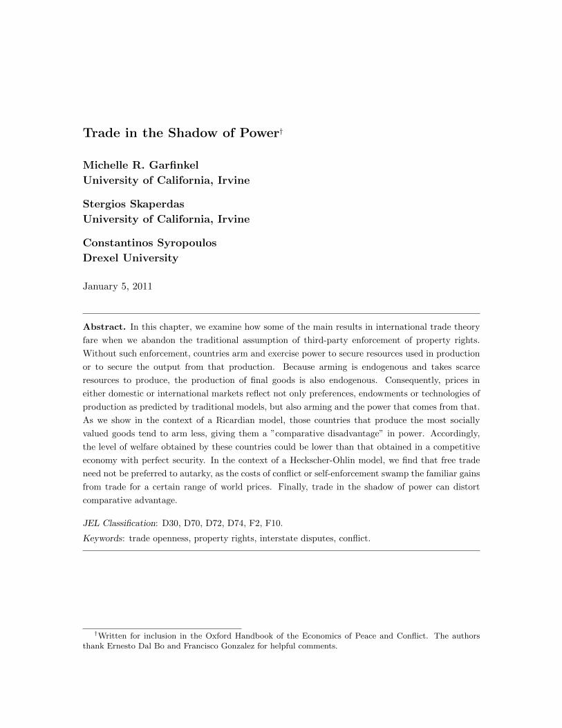
trade for both countries—namely, p ∈ (pA, p′)—as illustrated in Figure 1. For world prices

within this range, the payoffs for both countries under autarky are strictly greater than the

payoffs they enjoy under free trade; for world prices outside that range, p ≤ pA or p ≥ p′,

the payoffs for both countries under free trade are at least as high as the payoffs under

autarky.13 These findings are summarized in the following proposition:

Proposition 6. When the world price of oil is between pA and p′, welfare under autarkyis higher than welfare under free trade; otherwise, welfare under free trade is higher.

The intuition for these findings draws on the two key forces noted above: (i) the familiar

gains from trade and (ii) the induced (strategic) effects on arming and the associated costs

of insecurity. When the world price for oil (p) is less than the autarkic price (pA), the

production of guns under trade is lower. In this case, switching from an autarkic regime to

a free trade regime reduces each country’s incentive to contest the disputed resource. This

strategic effect represents a benefit that reinforces the familiar gains from trade to make

welfare unambiguously higher in a free-trade regime than that under autarky. However,

as the world price of oil rises and approaches pA, the conflict between the two nations

intensifies and the strategic benefit falls, as do the gains from trade. At the autarkic price,

the costs of insecurity are just as large under free trade as they are under autarky, so that

the strategic benefit from trade goes to zero along with the gains from trade. Thus, at

12Dal Bo and Dal Bo (2004 and this volume) and Garfinkel et al. (2008) yield an analogous finding in asetting with domestic insecurity.

13One can show further that the range of world prices under which autarky strictly dominates trade isincreasing in the degree of insecurity. The proof is similar to that of an analogous result shown Garfinkel etal. (2008), who consider among other things the effects of domestic conflict on the relative appeal of freetrade.

19

-

6

? p

V

V F (p)

V A pppppppppppppppp

ppppppppppppppppppp

ppppppppppppppppppp

s s

pA p′pmin

Figure 1: Welfare comparison

p = pA, welfare under autarky equals welfare under free trade, as shown in Figure 1.

As the world price rises above the autarkic level, the conflict between the two countries

intensifies further, implying that the strategic effect of trade generates a welfare cost relative

to the outcome under autarky (i.e., a higher burden of guns). Of course, at the same time,

the gains from trade rise above zero. However, these gains are swamped by the higher

burden of guns; thus, as the world price of oil rises above the autarkic price, welfare under

free trade falls below its autarkic level. Yet, as Proposition 6 indicates, when the world

price of oil becomes sufficiently high (p > p ′), the gains from winning the valuable land and

selling the oil in the global marketplace become very large and outweigh the welfare cost of

guns.

4 Concluding Remarks

Throughout most of human history, trade has taken place within insecure environments,

where property rights are not well defined or enforced—in both domestic and international

settings. While the costs borne by states, organizations, and individuals in trying to self-

enforce property rights are substantial, such costs and more generally the shadow of power

have not been formally incorporated into traditional economic thinking.

In this chapter, we have explored the robustness of some of the central results of tradi-

tional trade theory to power considerations between nations. The analysis has shown that

prices depend on arming and more generally power. This dependence implies in the context

of the augmented Ricardian model, contrary to traditional theory where power considera-

tions are ignored, that the country producing the more socially valued good faces a higher

20

opportunity cost of arming and thus a comparative disadvantage in power. In the context

of the augmented Heckscher-Ohlin model, this dependence has implications for the appeal

of free trade relative to that of autarky. Indeed, for some range of world prices, autarky will

be dominated by free trade. The analysis has shown further that, depending on the world

price, a country’s comparative advantage in the presence of insecurity might be opposite to

that predicted by the traditional theory that abstracts from insecurity.

Key to the analysis of both models is the level of security, represented by σ—a parameter

that we have treated as exogenous. An obviously important issue is what determines the

level of security. The continual fighting between England and France during the 18th century

took place mostly in the high seas and in their respective colonies. As such, only trade of

goods and resources that did not have to be transported by ship to-and-from the colonies

could be considered secure. The long nineteenth century that ended with the First World

War was relatively peaceful among the European powers. However, most international trade

then was taking place within each European power’s sphere of influence, and thus security

was not necessarily much greater than it had been in the 18th century. To be sure, not

many wars broke out during this period; but, there was considerable arming that accelerated

during the last two decades of that era. The gradual expansion of formal diplomacy, the

marriages and blood relations among European royalty, and perhaps emerging norms of

international conduct served as checks on the insecurity that existed then. After the Second

World War, these emerging norms along with the dismal experience of warfare crystallized

into a number of international organizations and institutions that significantly increased

perceived security in interstate relations. With the creation of the United Nations and the

collective security norms that developed, it became considerably harder for one country to

attack another, possibly resulting in a lower level of arming than what might have occurred

otherwise. The creation of the Steel and Coal Union that evolved into the current European

Union is another example of the organizations and institutions that dramatically increased

the level of security among some formerly mortal enemies. Whereas France and Germany

were such enemies before World War II, now there is no visible insecurity in any of the

resources and goods traded between them.

The level of security, then, depends on international institutions and norms that prevail

in any particular era. But security can also be expected to depend partly on the actions of

the states themselves vis-a-vis one another. By maintaining embassies, for example, in each

others’ capital, states can reduce the chance of accidental wars, and engage in confidence-

building measures that increase the perceived security of trade across them. The institution-

building that France and Germany and other European countries undertook after World

War II is an even more obvious example of the endogeneity of the level of security to the

actions of states. The process is not dissimilar to state-building by different factions within

21

countries as modeled by McBride et al. (2010).

Another type of state action, however, that can be deleterious to the security of any

two given states is the influence of third parties, usually states that can be considered

great powers. European countries that previously had high levels of contact and security

in their dealings before World War II, suddenly became enemies after the war because

they fell on either side of the divide created by the Cold War. That is not an historically

atypical condition. Before World War II, for example, smaller states in the periphery of the

European Great powers had to choose which Great power with whom to ally, a choice that

automatically implied that they would become enemies with neighbors who chose to ally

with a rival power.

More generally, even without consideration of third party intervention, alliance forma-

tion would seem to matter for security. As surveyed by Bloch (this volume), a number of

scholars have examined the determinants of alliances formation, but have not considered

explicitly the role of trade. We conjecture that different trade regimes imply potentially

different sets of stable alliances of countries, which is an important topic for future research.

References

Armington, Paul S. (1969), “A Theory of Demand for Products Distinguished by Place of

Production,” International Monetary Fund Staff Papers 16(1), 159–176.

Bloch, Francis (2010), “Endogenous Formation of Alliances in Conflicts,” this volume.

Chaudhuri, K.N. (1985), Trade and Civilisation in the Indian Ocean: An Economic History

from the Rise of Islam to 1750 (New York: Cambridge University Press).

Dal Bo, Ernesto and Pedro Dal Bo (2004), “Workers, Warriors, and Criminals: Social

Conflict in General Equilibrium,” Journal of the European Economic Association

(forthcoming).

Dal Bo, Ernesto and Pedro Dal Bo (2010), “Social Conflict and Policy in a Standard Trade

Model,” this volume.

Findlay, Ronald and Kevin O’Rourke (2007), Power and Plenty (Princeton, NJ: Princeton

University Press).

Findlay, Ronald and Kevin O’Rourke (2010), “War, Trade and Natural Resources: A

Historical Perspective,” this volume.

Garfinkel, Michelle R., Stergios Skaperdas, and Constantinos Syropoulos (2008), “Global-

ization and Domestic Conflict,” Journal of International Economics 76(2), 296–308.

22

Garfinkel, Michelle R., Stergios Skaperdas, and Constantinos Syropoulos (2010), “Trade

and Insecure Resources: Implications for Welfare and Comparative Advantage,” un-

published paper, University of California-Irvine.

Leeson, Peter T. (2009), The Invisible Hook: The Hidden Economics of Pirates (Princeton,

NJ: Princeton University Press).

McBride, Michael, Gary Milante and Stergios Skaperdas (2010) “War and Peace with

Endogenous State Capacity,” 2010, forthcoming, Journal of Conflict Resolution.

Ricardo, David (1817), The Principles of Political Economy and Taxation (London: Ev-

eryman’s Library, 1977).

Skaperdas, Stergios (1992), “Cooperation, Conflict, and Power in the Absence of Property

Rights, American Economic Review 82(4), 720–739.

Skaperdas, Stergios, and Constantinos Syropoulos (1997), “The Distribution of Income in

the Presence of Appropriative Activities,” Economica 64(253), 101–17.

Skaperdas, Stergios, and Constantinos Syropoulos (2001), “Guns, Butter, and Openness:

On the Relationship between Security and Trade,” American Economic Review: Pa-

pers and Proceedings 91(2), 353–357.

Stockholm International Peace Research Institute (2008), Yearbook 2008 Armaments,

Disarmament and International Security (Oxford: Oxford University Press).

A Appendix

Proof of proposition 1. Part (i) was established in the text, and part (ii) has been shown

in Skaperdas and Syropoulos (1997). However, we also prove part (ii) below in the proof to

the next proposition, as a special case.

Proof of proposition 2.

Part i. Suppose that RE = RS . Combining the two expressions in (14), we obtain the

following:

∂q∗

∂gE(RE − g∗E)(1− α)[σ(1− α) + (1− σ)(1− q∗)]

= − ∂q∗

∂gS(RS − g∗S)α[σα + (1 − σ)q∗]. (A.1)

Now suppose that g∗E > g∗S . Then we have the following:

23

• q∗ > 12 > 1− q∗;

• ∂q∗

∂gE< − ∂q∗

∂gS, when q(gE , gS) is concave (convex) in its first (second) argument, as is

the case with the Tullock form of the contest success function (3); and,

• RE − g∗E < RS − g∗S .

These three inequalities imply

∂q∗

∂gE(RE − g∗E)(1− α)[σ(1− α) + (1− σ)(1− q∗)]

< − ∂q∗

∂gS(RS − g∗S)(1 − α)[σ(1 − α) + (1 − σ)q∗]. (A.2)

But, (A.1) and (A.2) together imply,

− ∂q∗

∂gS(RS − g∗S)(1− α)[σ(1− α) + (1− σ)q∗]

> − ∂q∗

∂gS(RS − g∗S)α[σα + (1 − σ)q∗]. (A.3)

Since −∂q∗/∂gS > 0, this expression can hold if and only if

(1− α)[σ(1− α) + (1− σ)q∗] > α[σα+ (1− σ)q∗]⇔

(1− α)2σ + (1− α)(1− σ)q∗ > α2σ + α(1− σ)q∗ ⇔

(1− 2α)(1− σ)q∗ > [α2 − (1− α)2]σ.

This last inequality is only possible if α < 12 ; otherwise, the LHS would be non-positive and

the RHS would be non-negative, thus negating the strict inequality.

Parts ii and iii. For notational convenience, let Vi ≡ Vi(gE , gS) for i = E,S and β ≡σ/(1−σ). In what follows, we sometimes omit the equilibrium symbol “∗” to avoid clutter,

but one should keep in mind that functions are to be evaluated at the Nash equilibrium.

The optimizing choices of gE and gS must satisfy respectively the following conditions:

∂VE∂gE

= VE

[∂q∂gE

βα+ q− α

RE − gE

]= 0 (A.4a)

∂VS∂gS

= VS

[− ∂q∂gS

β(1− α) + (1− q)− 1− αRS − gS

]= 0. (A.4b)

Using the specification of the CSF shown in (3) and letting G = gE + gS ,14 we can rewrite

14We use this particular specification to keep matters as simple as possible; however, the results hold more

24

gE and gS as gE = qG and gS = (1 − q)G, respectively. Furthermore, the specification in

(3) implies that ∂q/∂gE = (1− q)/G and ∂q/∂gS = −q/G. Substituting these relationships

into (A.4a) and (A.4b) yields the following:

(1− q)/Gβα+ q

− α

RE − qG= 0 (A.5a)

q/G

β(1− α) + 1− q− 1− αRS − (1− q)G

= 0. (A.5b)

Now solve (A.5a) and (A.5b) for G and label the resulting solutions GE and GS , respectively.

Then, for given factor endowments RE and RS , define

Φ(q, α, β) ≡ GE − GS

=(1− q)RE

q(α+ 1− q) + α2β− qRS

(1− q)(1− α+ q) + (1− α)2β. (A.6)

Φ is continuous in q, limq→0 Φ = RE/(α2β) > 0, and limq→1 Φ = −RS/[(1−α)2β] < 0; there-

fore, by the implicit function theorem, there exists a q∗ = q∗(α, β) such that Φ(q∗, α, β) = 0.

Differentiating Φ with respect to q, α and β gives respectively,

Φq = −

RE[α+ α2β + (1− q)2

][q(α+ 1− q) + α2β]2

+RS[1− α+ (1− α)2β + q2

][(1− q)(1− α+ q) + (1− α)2β]2

(A.7a)

Φα = −RE(1− q)(q + 2αβ)

[q(α+ 1− q) + α2β]2+

RSq [1− α+ 2(1− α)β]

[(1− q)(1− α+ q) + (1− α)2β]2

(A.7b)

Φβ = − REα2(1− q)

[q(α+ 1− q) + α2β]2+

RS(1− α)2q

[(1− q)(1− α+ q) + (1− α)2β]2. (A.7c)

Notice that the sign of Φβ is ambiguous, whereas the signs of Φq and Φα are both negative.

Moreover, since Φq < 0, the equilibrium share q∗ is unique.

Now, consider how q∗ responds to an exogenous increase in α. By the implicit function

theorem, we have dq∗/dα = −Φα/Φq. Since Φα and Φq are both negative, dq∗/dα < 0

for all α ∈ (0, 1), which establishes part (ii) of the proposition, and suggests that g∗E falls

relative to g∗S as α rises.

This finding, however, does not necessarily imply that g∗E is decreasing or that g∗S is

increasing in α. Consider the influence of an exogenous increase in α on g∗E , for exam-

ple, noting that G∗ = GE∗, which implies g∗E = q∗GE∗. Differentiation of g∗E = q∗GE∗

generally.

25

appropriately yields the following:

dg∗Edα

= qdG∗

dα+

(G∗ + q

dG∗

dq

)dq∗

dα= q

dG∗

dα+

(G∗ + q

dG∗

dq

)[−Φα

Φq

]= −REq(1− q)(q + 2αβ)

[q(α+ 1− q) + α2β]2+REα

[q2 + (2q − 1)αβ

][q(α+ 1− q) + α2β]2

[Φα

Φq

].

Generally, this expression cannot be signed. However, it is worth considering what happens

in the case of complete insecurity, where σ = 0 and thus β = 0 (Proposition 2(ii)). In this

case, the expression above simplifies as follows:

dg∗Edα

∣∣∣∣β=0

= − RE(1− q)(α+ 1− q)2

+REα

(α+ 1− q)2

RE(1−q)q(α+1−q)2 + RSq

(1−q)(1−α+q)2RE [α+(1−q)2]q2(α+1−q)2 + RS [1−α+q2]

(1−q)2(1−α+q)2

= − REΘ

(α+ 1− q)2Φq, (A.8)

where15

Θ = −[RE(1− q)2

q2(α+ 1− q)− RS(1− α− αq + q2)

(1− q)(1− α+ q)2

]= − 2(1− α)G

q(1− α+ q)< 0.

Since −Φq > 0 and q ≤ 1, the sign of the expression in (A.8) equals the sign of Θ, which

is negative as indicated above. Thus, when σ = 0, an increase in α implies a decrease in

g∗E . Analogous calculations show that an increase in α implies an increase in g∗S . Hence, an

exogenous increase in α induces a decrease in q∗.

Turning to the effects of a change in security σ and thus β = σ/(1− σ), first note that,

since the sign of Φβ is ambiguous, we cannot sign dq∗/dβ = −Φβ/Φq. However, we can

sign the effect of an exogenous change in security on arming by both countries. To proceed,

recall that G∗ = GE∗, which implies g∗E = q∗GE∗. Now differentiate the latter expression

to obtain

dg∗Edβ

= qdG∗

dβ+

(G∗ +

dG∗

dq

)dq∗

dβ= q

dG∗

dβ+

(G∗ +

dG∗

dq

)[−

Φβ

Φq

]= − REα

2q(1− q)[q(α+ 1− q) + α2β]2

−REα

[q2 + α(2q − 1)β

][q(α+ 1− q) + α2β]2

[Φβ

Φq

].

15The second equality below can be verified by using the definitions of GE∗ and GS∗ (both of which equalG∗ in equilibrium) given in connection with (A.6) to eliminate RE and RS .

26

Simplifying leads us to conclude that sign(dg∗E/dβ) = −sign(Ω), where

Ω ≡ REα(1− q)2

q(α+ 1− q) + α2β+RSq[(1− α)2q(q + αβ) + α(1− α+ q2)(1− q)]

[(1− q)(1− α+ q) + (1− α)2β]2> 0.

It follows that dg∗E/dβ < 0. Similar calculations show that dg∗S/dβ < 0. Hence, an increase

in security (σ and thus β) unambiguously reduces arming by both countries, as claimed in

part (iii) in the proposition.

Proof of Proposition 3.

Part i: Let Zk ≡ (RE − gE)α(RS − gS)1−α denote the total surplus under security regime

k (= 1, ∗) and observe that, from Proposition 2(iii), Z∗ < Z1. Focusing on i = E, to prove

the first point, it is sufficient to show that, for any σ ∈ [0, 1), limα→0 V∗E > limα→0 V

1E . This

sufficiency is so for the following reason. Since, as was noted in the text above, V ∗E < V 1E

for α = 12 and equilibrium payoffs are continuous in α, the inequality implies that there

will exist an α ∈ (0, 12) such that V ∗E = V 1E for α = α and V ∗E > V 1

E for all α ∈ [0, α).

Furthermore, since Zk = V kE + V k

S and Z∗ < Z1, it follows that V ∗S < V 1S for all α ∈ [0, α).

By the same logic, we also can establish the existence of an ˜α ∈ (12 , 1) such that V ∗S = V 1S

for α = ˜α, with V ∗S > V 1S and V ∗E < V 1

E for all α ∈ ( ˜α, 1].)

To proceed, let bS(gE) and bE(gS) denote the best-response functions of countries S

and E, respectively. It is straightforward to verify from (14) that, as α→ 0, the functions

satisfy the following

bS(gE) = max(0,√

(1− σ)gE(gE +RS)− gE)

whereas bE(gS) = RE for gS > 0 and bE(0) equals any gE ∈ (0, RE ].16 One can verify now

that the Nash equilibrium in guns is given by:

(g∗E , g∗S) =

(RE ,√

(1− σ)RE(RE +RS)−RE) if σ ∈[0, RS

RE+RS

];

(1−σσ RS , 0) if σ ∈(

RSRE+RS

, 1).

(A.9)

Substituting these values into (7a) with α = 0 yields the following equilibrium welfare value

for country i = E:

limα→0

V ∗E =

RE(1− σ)(√

RE+RSRE(1−σ) − 1

)if σ ∈

[0, RS

RE+RS

];

RS(1− σ) if σ ∈(

RSRE+RS

, 1).

(A.10)

16Recalling that β ≡ σ/(1 − σ), the definition of bS(gE) reveals that bS(gE) > 0 for all gE ∈ (0, RS/β)and bS(gE) = 0 for all other gE values.

27

Notice that limα→0

V ∗E > 0 for all resource endowments and σ ∈ [0, 1). By contrast, from (8a)

with α = 0, limα→0

V 1E = 0. Thus, lim

α→0V ∗E > lim

α→0V 1E for σ ∈ [0, 1).

Part ii: That V ∗E is not necessarily increasing in security (σ) follows from inspection of

the first part of (A.10), which reveals that, in the neighborhood of α = 0, V ∗E could be

decreasing, increasing or non-monotonic in σ for σ ≤ RSRE+RS

.

28