Embed Size (px)
DESCRIPTION
OVERVIEW Typical & atypical distributions Two new fitting methods An interesting new case Potential impact & a wish list . Multimodal fitting of atypical size distributions from AERONET Michael Taylor Stelios Kazadzis Evangelos Gerasopoulos URL: http://apcg.meteo.noa.gr - PowerPoint PPT Presentation
Citation preview
Michael Taylor, COMECAP 29th May, 2014: Remote Sensing Session
Multimodal fitting of atypical size distributions from AERONET
Michael Taylor Stelios KazadzisEvangelos Gerasopoulos
URL: http://apcg.meteo.noa.greMail: [email protected]
OVERVIEW 1. Typical & atypical distributions 2. Two new fitting methods3. An interesting new case4. Potential impact & a wish list
1. Typical & atypical distributions
Michael Taylor, COMECAP 29th May, 2014: Remote Sensing Session
Michael Taylor, COMECAP 29th May, 2014: Remote Sensing Session
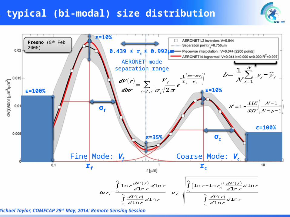
Fresno (8th Feb 2006)
0.439 ≤ rs ≤ 0.992μm
AERONET modeseparation range
rf rc
σf
σc
Fine Mode: Vf Coarse Mode: Vc
𝒅𝑽 (𝒓 )𝒅𝒍𝒏𝒓
= ∑𝒊= 𝒇 ,𝒄
𝑽 𝒊
𝝈 𝒊√𝟐𝝅𝒆−𝟏𝟐 ( 𝒍𝒏𝒓 −𝒍𝒏𝒓 𝒊
𝝈𝒊)𝟐
1a) A typical (bi-modal) size distribution
𝐥𝐧𝒓 𝒊=∫𝑟1
𝑟2
ln 𝑟𝑑𝑉 (𝑟 )𝑑 ln 𝑟
𝑑 ln𝑟
∫𝑟 1
𝑟2 𝑑𝑉 (𝑟 )𝑑 ln 𝑟
𝑑 ln𝑟
𝝈𝒊=√∫𝑟 1𝑟 2
( ln𝑟 − ln 𝑟 𝑖 )2 𝑑𝑉 (𝑟 )𝑑 ln 𝑟
𝑑 ln 𝑟
∫𝑟1
𝑟2 𝑑𝑉 (𝑟 )𝑑 ln 𝑟
𝑑 ln 𝑟
𝑏= 1𝑁∑
𝑖=1
𝑁
𝑦 𝑖− 𝑦 𝑖
𝑅2=1−𝑆𝑆𝐸𝑆𝑆𝑇 ( 𝑁−1
𝑁−𝑝−1 )
ε=35%
ε=10%
ε=10%ε=100%
ε=100%
Michael Taylor, COMECAP 29th May, 2014: Remote Sensing Session
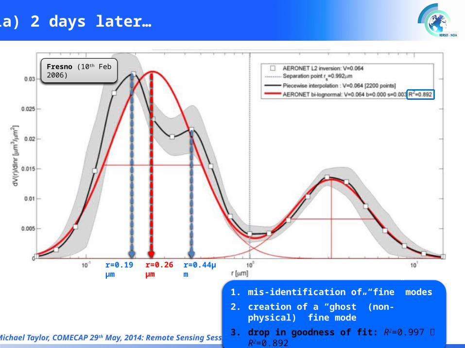
1a) 2 days later…
r=0.19μm r=0.44μmr=0.26μm
1. mis-identification of “fine” modes
2. creation of a “ghost” (non-physical) fine mode
3. drop in goodness of fit: R2=0.997 R2=0.892
Fresno (10th Feb 2006)
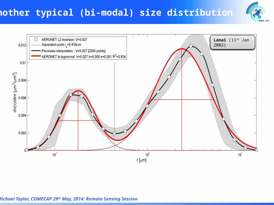
1a) another typical (bi-modal) size distribution
Michael Taylor, COMECAP 29th May, 2014: Remote Sensing Session
Lanai (11th Jan 2002)
Michael Taylor, COMECAP 29th May, 2014: Remote Sensing Session
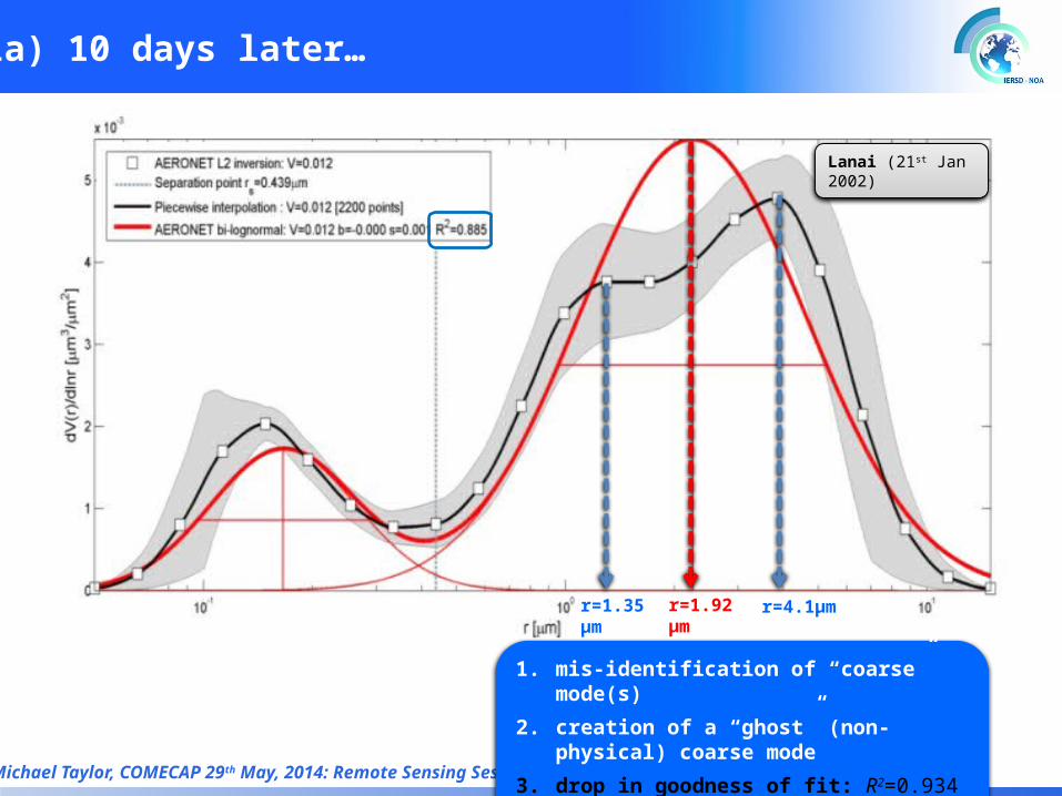
1a) 10 days later…
r=1.35μm r=4.1μmr=1.92μm
1. mis-identification of “coarse” mode(s)
2. creation of a “ghost” (non-physical) coarse mode
3. drop in goodness of fit: R2=0.934 R2=0.885
Lanai (21st Jan 2002)
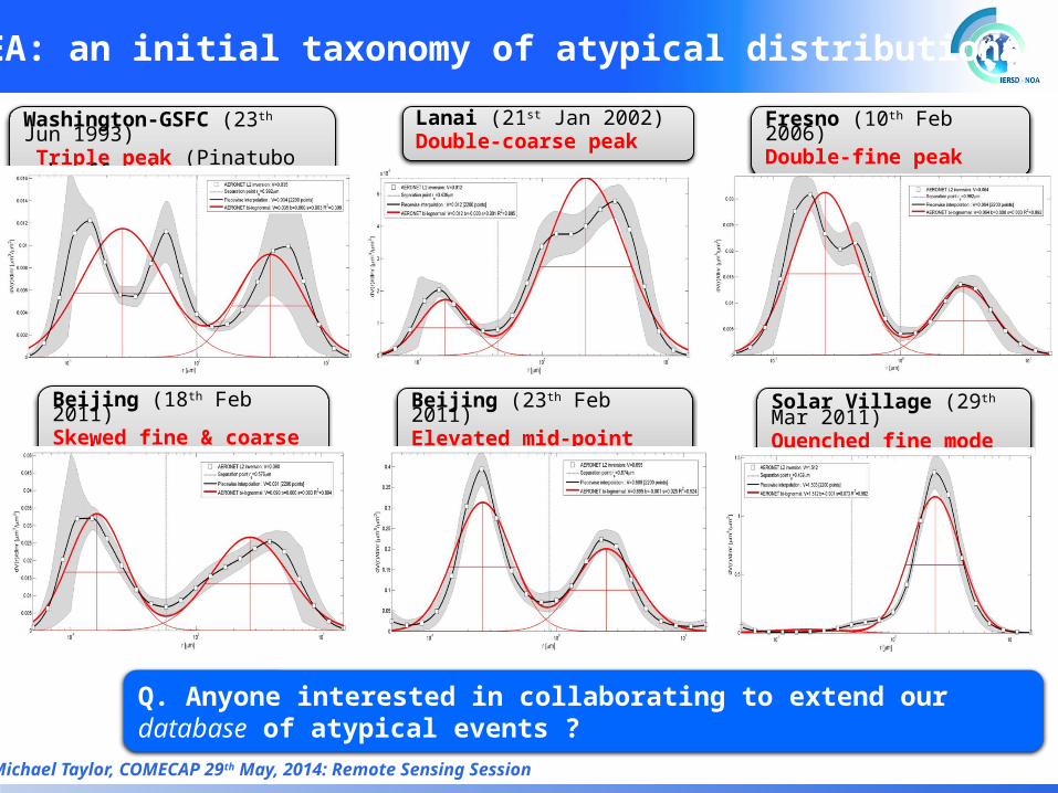
1b) IDEA: an initial taxonomy of atypical distributions
Michael Taylor, COMECAP 29th May, 2014: Remote Sensing Session
Lanai (21st Jan 2002)Double-coarse peak
Fresno (10th Feb 2006)Double-fine peak
Washington-GSFC (23th Jun 1993) Triple peak (Pinatubo ash effect)
Solar Village (29th Mar 2011)Quenched fine mode
Beijing (18th Feb 2011)Skewed fine & coarse peaks
Beijing (23th Feb 2011)Elevated mid-point
Q. Anyone interested in collaborating to extend our database of atypical events ?
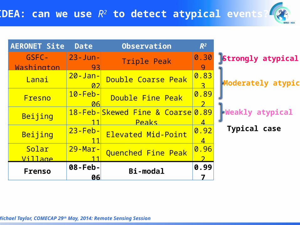
1c) IDEA: can we use R2 to detect atypical events?
Michael Taylor, COMECAP 29th May, 2014: Remote Sensing Session
AERONET Site Date Observation R2
GSFC-Washington 23-Jun-93 Triple Peak 0.309
Lanai 20-Jan-02 Double Coarse Peak 0.833
Fresno 10-Feb-06 Double Fine Peak 0.892
Beijing 18-Feb-11 Skewed Fine & Coarse Peaks 0.894
Beijing 23-Feb-11 Elevated Mid-Point 0.924
Solar Village 29-Mar-11 Quenched Fine Peak 0.962
Frenso 08-Feb-06 Bi-modal 0.997 Typical case
Strongly atypical
Moderately atypical
Weakly atypical
2. Two new fitting methods
Michael Taylor, COMECAP 29th May, 2014: Remote Sensing Session
Taylor, Kazadzis, Gerasopoulous (2014): AMT 7, 839-858
Michael Taylor, COMECAP 29th May, 2014: Remote Sensing Session
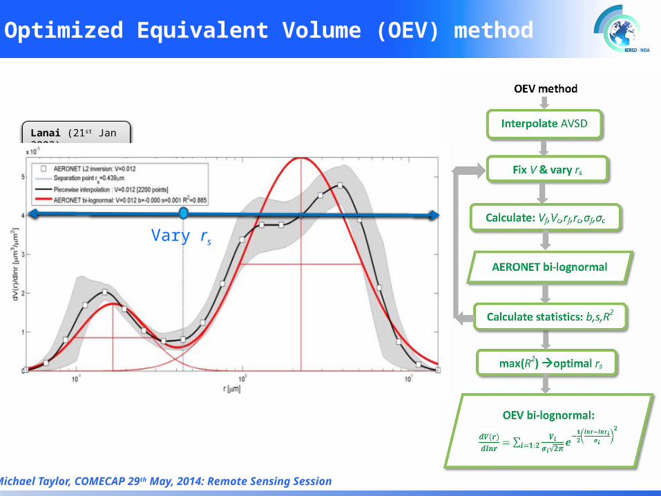
2a) Optimized Equivalent Volume (OEV) method
Lanai (21st Jan 2002)
Vary rs
Michael Taylor, COMECAP 29th May, 2014: Remote Sensing Session
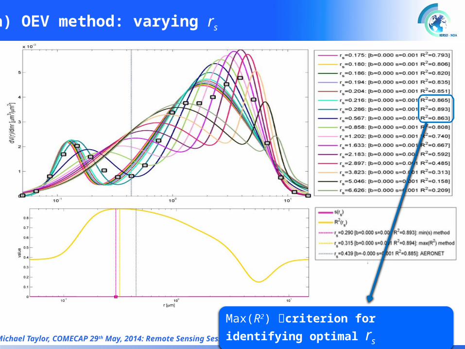
2a) OEV method: varying rs
Max(R2) criterion for identifying optimal rs
Michael Taylor, COMECAP 29th May, 2014: Remote Sensing Session
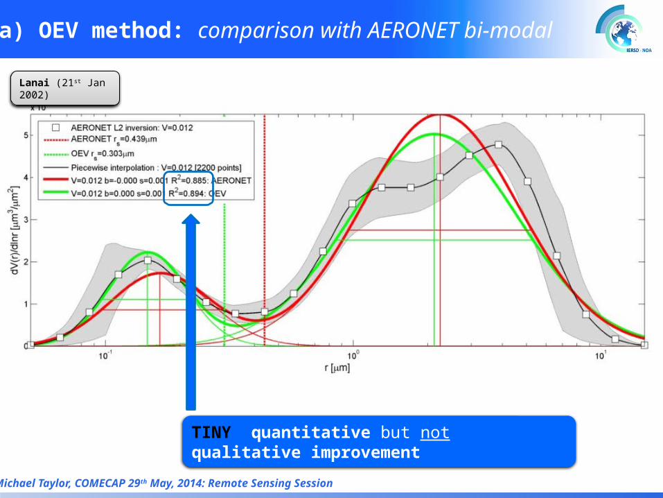
2a) OEV method: comparison with AERONET bi-modal
TINY quantitative but not qualitative improvement
Lanai (21st Jan 2002)
Michael Taylor, COMECAP 29th May, 2014: Remote Sensing Session
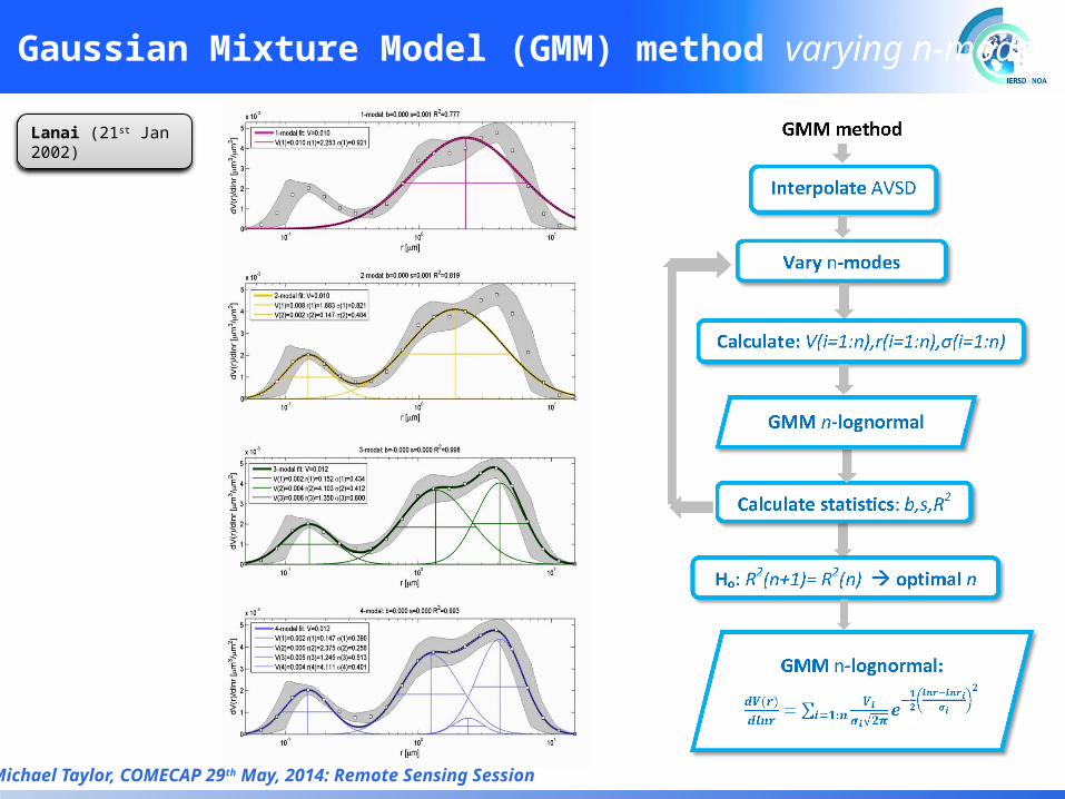
2b) Gaussian Mixture Model (GMM) method varying n-modes
Lanai (21st Jan 2002)
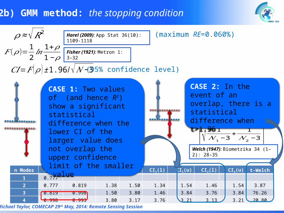
n Modes R2(n) R2(n+1) F(ρ1) F(ρ2) CI1(l) CI1(u) CI2(l) CI2(u) t-Welch1 0.7772 0.777 0.819 1.38 1.50 1.34 1.54 1.46 1.54 3.873 0.819 0.998 1.50 3.80 1.46 3.84 3.76 3.84 76.264 0.998 0.993 3.80 3.17 3.76 3.21 3.13 3.21 20.80
Michael Taylor, COMECAP 29th May, 2014: Remote Sensing Session
2b) GMM method: the stopping condition
𝐹 (𝜌)=12𝑙𝑛1+𝜌1− 𝜌
𝜌 ≈√𝑅2
𝐶𝐼=𝐹 (𝜌 )±1.96/√𝑁−3
𝑡=| 𝐹 (𝜌1 )−𝐹 (𝜌2 )
√ 1𝑁1−3
+ 1𝑁2−3
|
Fisher (1921): Metron 1: 3–32
Welch (1947): Biometrika 34 (1–2): 28–35
(maximum RE=0.060%)
(95% confidence level)
CASE 1: Two values of (and hence R2) show a significant statistical difference when the lower CI of the larger value does not overlap the upper confidence limit of the smaller value
CASE 2: In the event of an overlap, there is a statistical difference when t>1.96
Harel (2009): App Stat 36(10): 1109-1118
Michael Taylor, COMECAP 29th May, 2014: Remote Sensing Session
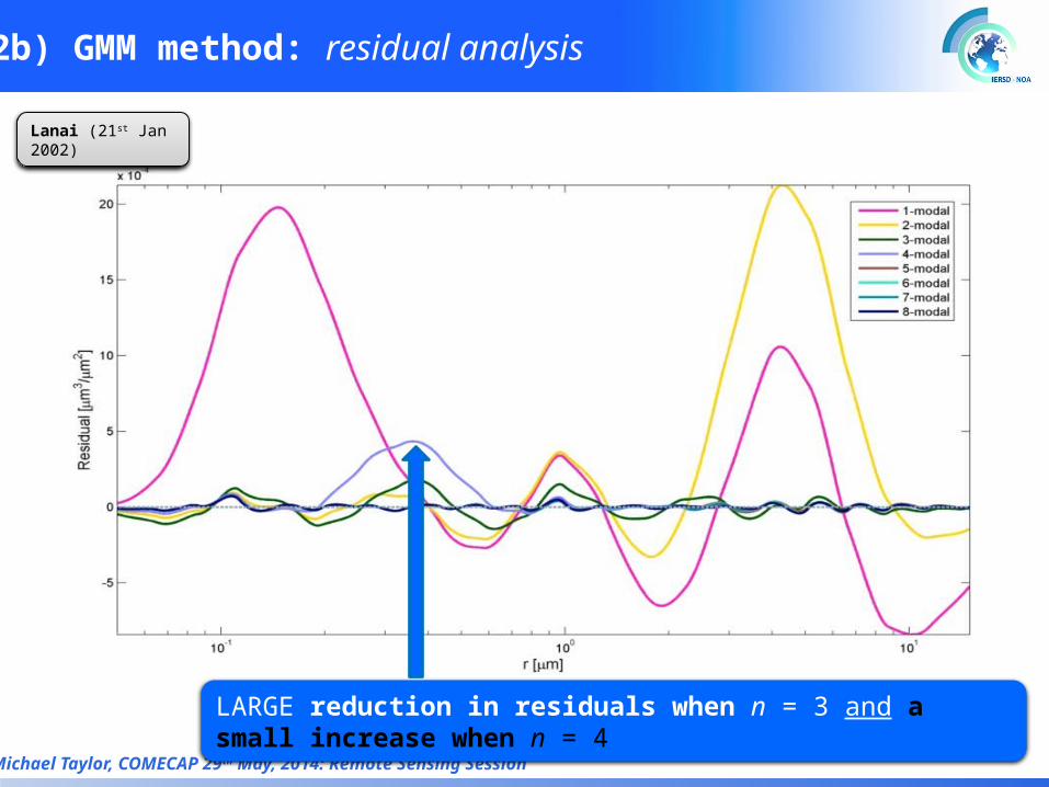
2b) GMM method: residual analysis
LARGE reduction in residuals when n = 3 and a small increase when n = 4
Lanai (21st Jan 2002)
Michael Taylor, COMECAP 29th May, 2014: Remote Sensing Session
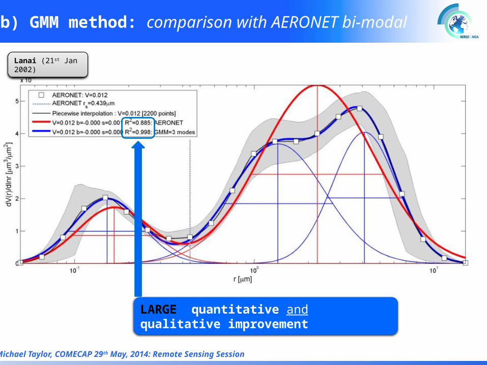
2b) GMM method: comparison with AERONET bi-modal
LARGE quantitative and qualitative improvement
Lanai (21st Jan 2002)
3. An interesting new case
Michael Taylor, COMECAP 29th May, 2014: Remote Sensing Session
Michael Taylor, COMECAP 29th May, 2014: Remote Sensing Session
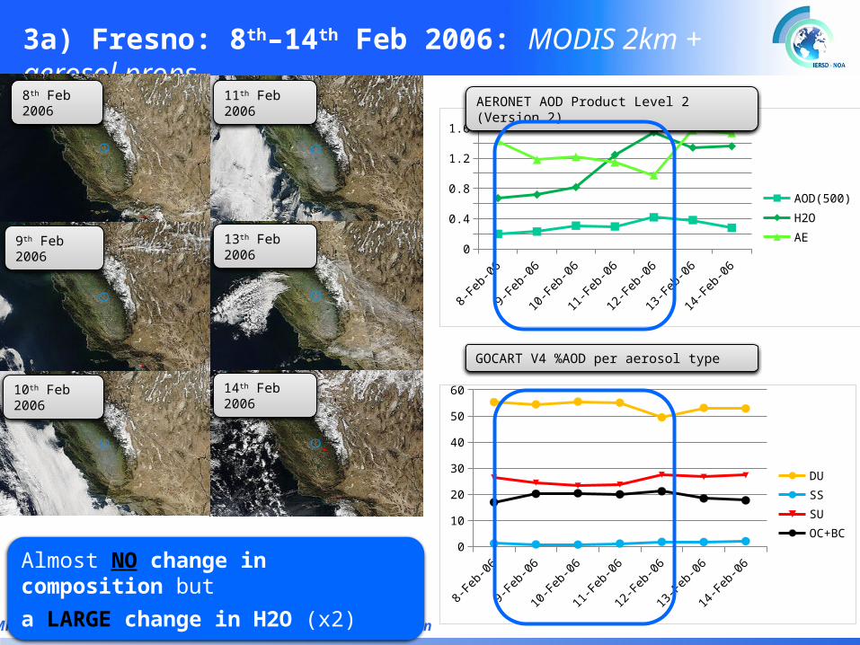
3a) Fresno: 8th–14th Feb 2006: MODIS 2km + aerosol props.
11th Feb 2006
13th Feb 2006
14th Feb 2006
9th Feb 2006
10th Feb 2006
8th Feb 2006
8-Feb-06
9-Feb-06
10-Feb-06
11-Feb-06
12-Feb-06
13-Feb-06
14-Feb-06
00.20.40.60.8
11.21.41.61.8
AOD(500)H2OAE
AERONET AOD Product Level 2 (Version 2)
0
10
20
30
40
50
60
DUSSSUOC+BC
GOCART V4 %AOD per aerosol type
Almost NO change in composition but
a LARGE change in H2O (x2)
Michael Taylor, COMECAP 29th May, 2014: Remote Sensing Session
8th Feb
9th Feb
10th Feb
11th Feb
13th Feb
14th Feb
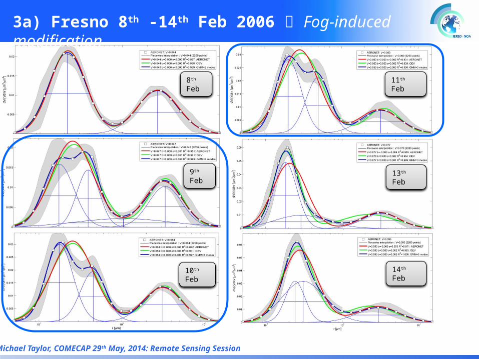
3a) Fresno 8th -14th Feb 2006 Fog-induced modification
4. Potential impacts
Michael Taylor, COMECAP 29th May, 2014: Remote Sensing Session
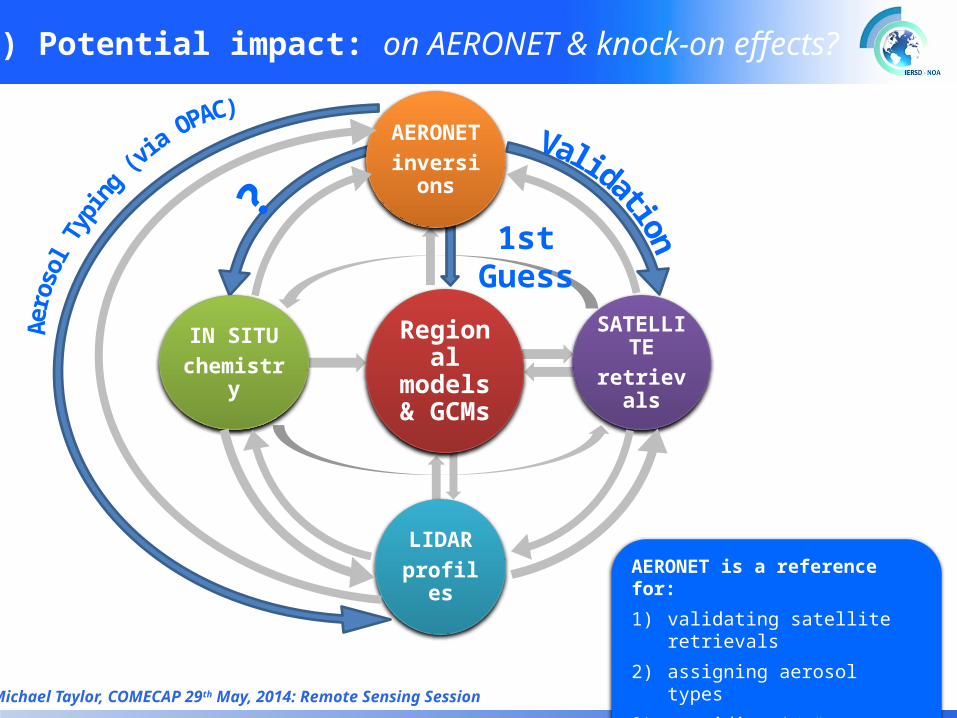
4b) Potential impact: on AERONET & knock-on effects?
Michael Taylor, COMECAP 29th May, 2014: Remote Sensing Session
Regional models & GCMs
AERONETinversions
SATELLITEretrievals
LIDARprofiles
IN SITUchemistry
1st Guess
AERONET is a reference for:
1) validating satellite retrievals
2) assigning aerosol types
3) providing 1st guesses in “spin-ups”
Michael Taylor, COMECAP 29th May, 2014: Remote Sensing Session
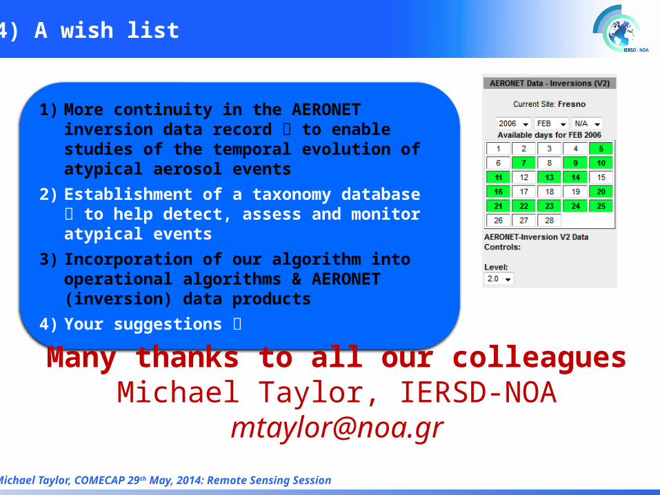
4) A wish list
1) More continuity in the AERONET inversion data record to enable studies of the temporal evolution of atypical aerosol events
2) Establishment of a taxonomy database to help detect, assess and monitor atypical events
3) Incorporation of our algorithm into operational algorithms & AERONET (inversion) data products
4) Your suggestions
Many thanks to all our colleaguesMichael Taylor, IERSD-NOA
EXTRA SLIDES
Michael Taylor, COMECAP 29th May, 2014: Remote Sensing Session
Michael Taylor, COMECAP 29th May, 2014: Remote Sensing Session
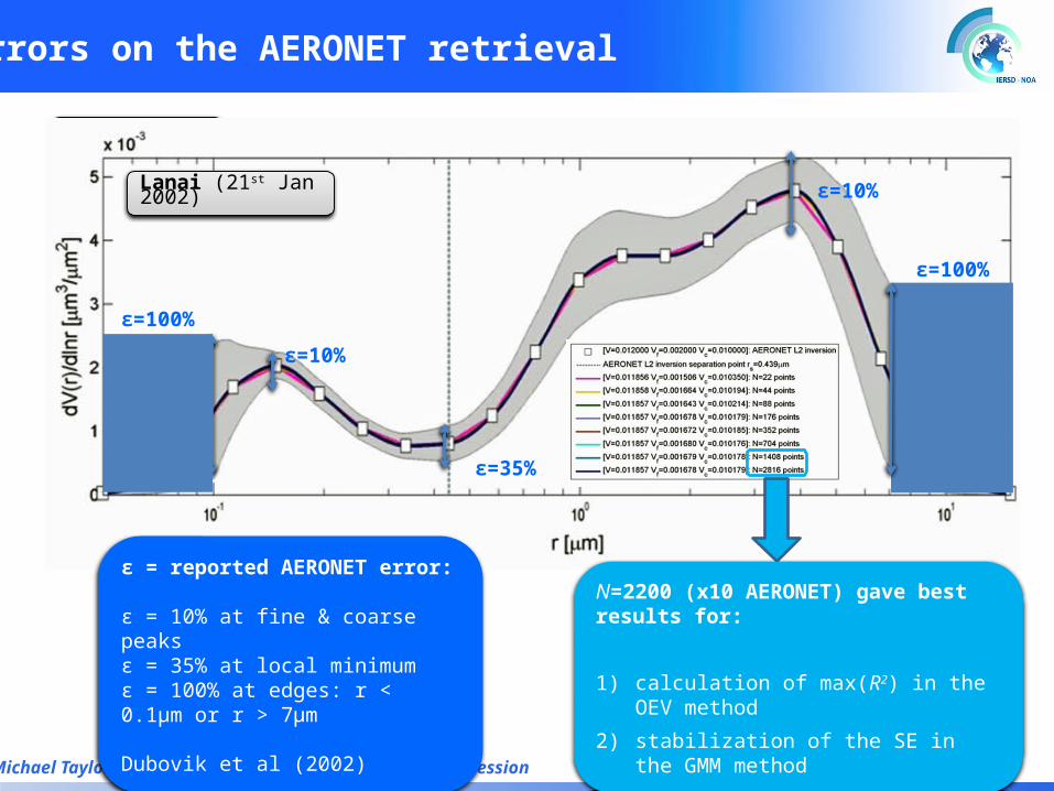
Errors on the AERONET retrieval
Lanai (21st Jan 2002)
ε=100%
ε=10%
ε=10%
ε=35%
ε=100%
ε = reported AERONET error:
ε = 10% at fine & coarse peaksε = 35% at local minimumε = 100% at edges: r < 0.1μm or r > 7μm
Dubovik et al (2002)
Lanai (21st Jan 2002)
N=2200 (x10 AERONET) gave best results for:
1) calculation of max(R2) in the OEV method
2) stabilization of the SE in the GMM method
Michael Taylor, COMECAP 29th May, 2014: Remote Sensing Session
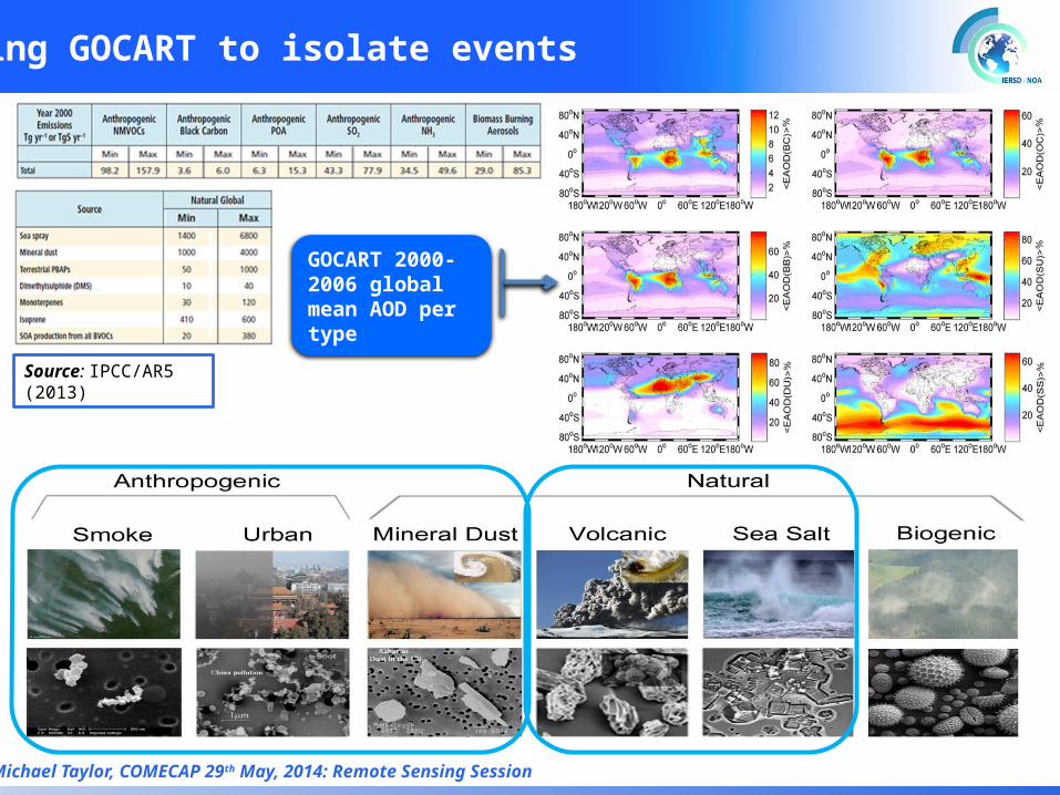
Using GOCART to isolate events
Source: IPCC/AR5 (2013)
GOCART 2000-2006 global mean AOD per type
Michael Taylor, COMECAP 29th May, 2014: Remote Sensing Session
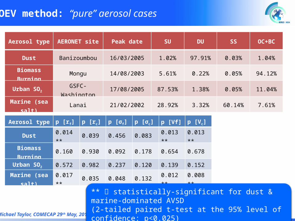
Aerosol type AERONET site Peak date SU DU SS OC+BC
Dust Banizoumbou 16/03/2005 1.02% 97.91% 0.03% 1.04%
Biomass Burning Mongu 14/08/2003 5.61% 0.22% 0.05% 94.12%
Urban SO2 GSFC-Washington 17/08/2005 87.53% 1.38% 0.05% 11.04%
Marine (sea salt) Lanai 21/02/2002 28.92% 3.32% 60.14% 7.61%
Aerosol type p [rf] p [rc] p [σf] p [σc] p [Vf] p [Vc]
Dust 0.014 ** 0.039 0.456 0.083 0.013 ** 0.013 **
Biomass Burning 0.160 0.930 0.092 0.178 0.654 0.678
Urban SO2 0.572 0.982 0.237 0.120 0.139 0.152
Marine (sea salt) 0.017 ** 0.035 0.048 0.132 0.012 ** 0.008 **
** statistically-significant for dust & marine-dominated AVSD (2-tailed paired t-test at the 95% level of confidence: p<0.025)
OEV method: “pure” aerosol cases
Michael Taylor, COMECAP 29th May, 2014: Remote Sensing Session
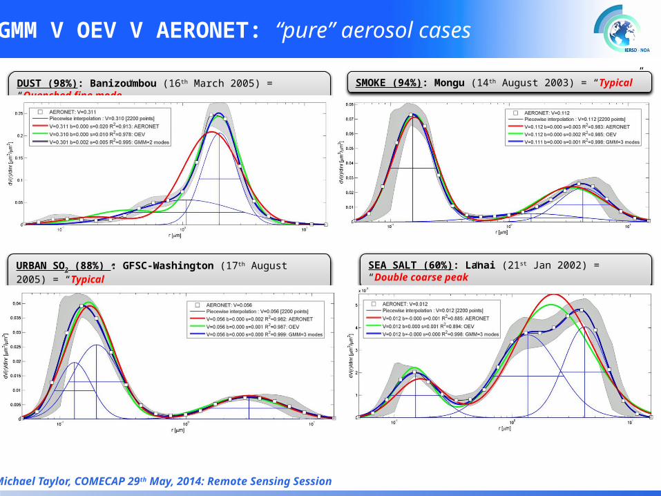
GMM V OEV V AERONET: “pure” aerosol cases
SEA SALT (60%): Lanai (21st Jan 2002) = “Double coarse peak”
DUST (98%): Banizoumbou (16th March 2005) = “Quenched fine mode”
URBAN SO2 (88%) : GFSC-Washington (17th August 2005) = “Typical”
SMOKE (94%): Mongu (14th August 2003) = “Typical”
Michael Taylor, COMECAP 29th May, 2014: Remote Sensing Session
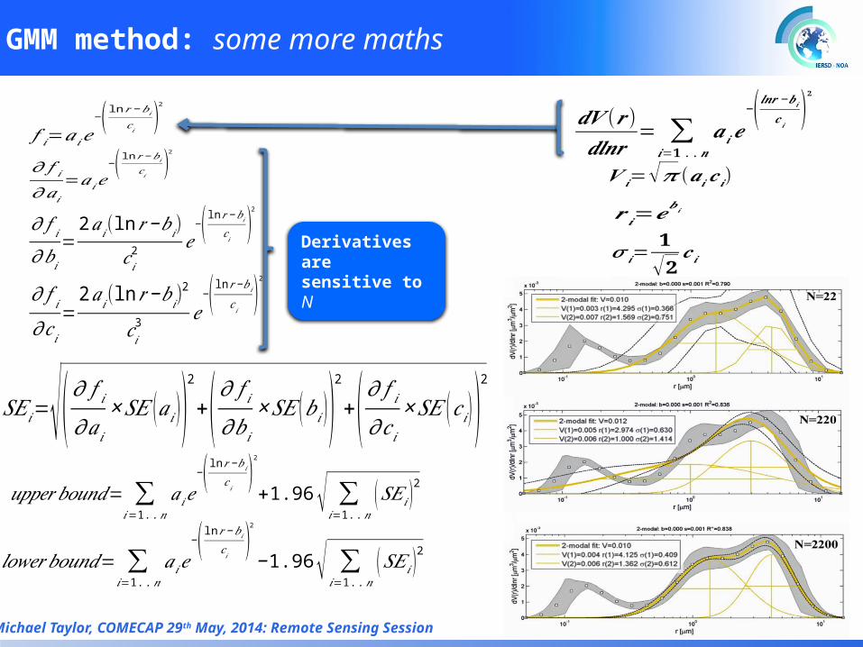
𝑆𝐸 𝑖=√(𝜕 𝑓 𝑖𝜕𝑎𝑖×𝑆𝐸 (𝑎𝑖 ))
2
+(𝜕 𝑓 𝑖𝜕𝑏𝑖
×𝑆𝐸 (𝑏𝑖 ))2
+(𝜕 𝑓 𝑖𝜕𝑐𝑖×𝑆𝐸 (𝑐𝑖 ))
2
𝑓 𝑖=𝑎𝑖𝑒−( ln 𝑟−𝑏𝑖
𝑐 𝑖)2
𝜕 𝑓 𝑖
𝜕𝑎𝑖
=𝑎𝑖𝑒−( ln 𝑟−𝑏𝑖
𝑐 𝑖)2
𝜕 𝑓 𝑖
𝜕𝑏𝑖
=2𝑎𝑖 (ln 𝑟 −𝑏𝑖)
𝑐 𝑖2 𝑒
−( ln 𝑟−𝑏𝑖
𝑐 𝑖)2
𝜕 𝑓 𝑖
𝜕𝑐 𝑖
=2𝑎𝑖 (ln 𝑟 −𝑏𝑖)
2
𝑐𝑖3 𝑒
−( ln 𝑟−𝑏𝑖
𝑐 𝑖)2
𝑢𝑝𝑝𝑒𝑟 𝑏𝑜𝑢𝑛𝑑= ∑𝑖=1. .𝑛
𝑎𝑖𝑒−( ln 𝑟 −𝑏𝑖
𝑐 𝑖)2
+1.96 √ ∑𝑖=1. .𝑛
(𝑆𝐸𝑖 )2
𝑙𝑜𝑤𝑒𝑟 𝑏𝑜𝑢𝑛𝑑= ∑𝑖=1. .𝑛
𝑎𝑖𝑒−( ln 𝑟 −𝑏𝑖
𝑐 𝑖)2
−1.96√ ∑𝑖=1. .𝑛
(𝑆𝐸 𝑖 )2
Derivatives are sensitive to N
𝒅𝑽 (𝒓 )𝒅𝒍𝒏𝒓
= ∑𝒊=𝟏..𝒏
𝒂𝒊𝒆−( 𝒍𝒏𝒓 −𝒃𝒊
𝒄𝒊)𝟐
𝑽 𝒊=√𝝅 (𝒂𝒊𝒄 𝒊)
𝒓 𝒊=𝒆𝒃𝒊
𝝈𝒊=𝟏√𝟐
𝒄 𝒊
GMM method: some more maths
Michael Taylor, COMECAP 29th May, 2014: Remote Sensing Session
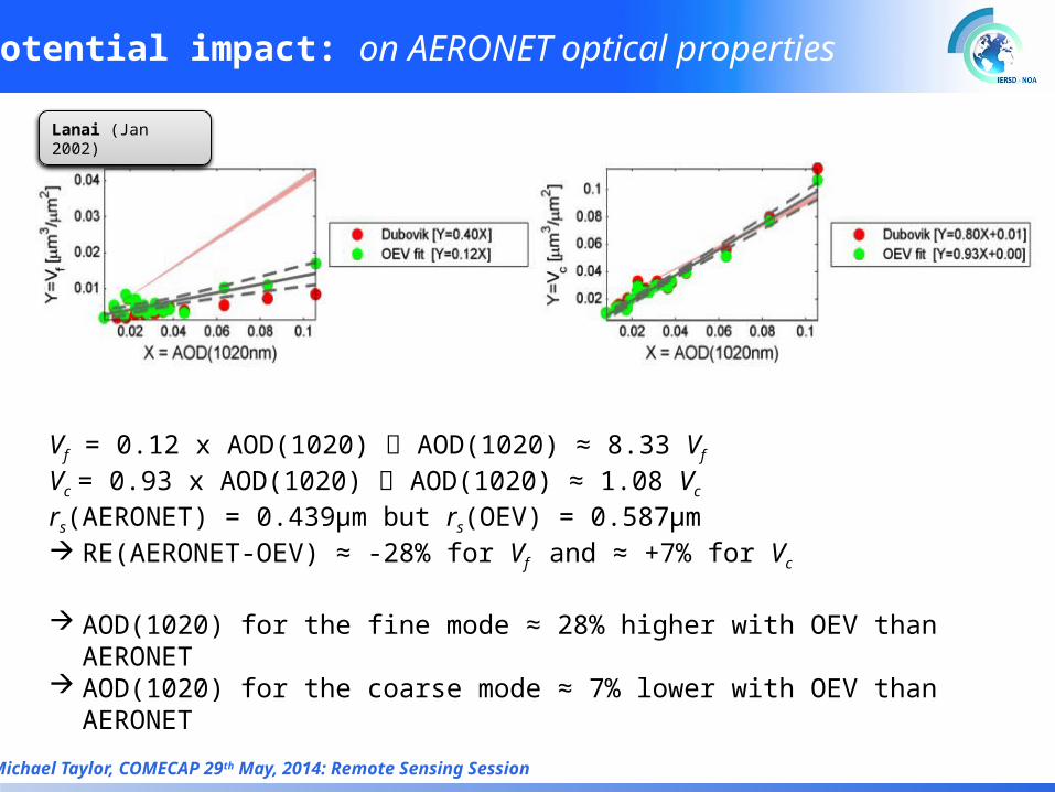
Potential impact: on AERONET optical properties
Lanai (Jan 2002)
Vf = 0.12 x AOD(1020) AOD(1020) ≈ 8.33 Vf
Vc = 0.93 x AOD(1020) AOD(1020) ≈ 1.08 Vc
rs(AERONET) = 0.439µm but rs(OEV) = 0.587µm RE(AERONET-OEV) ≈ -28% for Vf and ≈ +7% for Vc
AOD(1020) for the fine mode ≈ 28% higher with OEV than AERONET AOD(1020) for the coarse mode ≈ 7% lower with OEV than AERONET
Michael Taylor, COMECAP 29th May, 2014: Remote Sensing Session
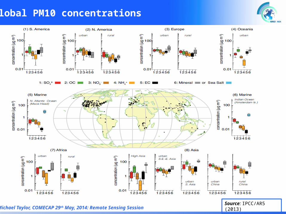
Global PM10 concentrations
Source: IPCC/AR5 (2013)
Michael Taylor, COMECAP 29th May, 2014: Remote Sensing Session
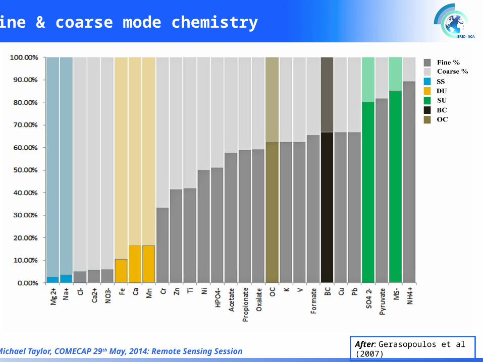
Fine & coarse mode chemistry
After: Gerasopoulos et al (2007)
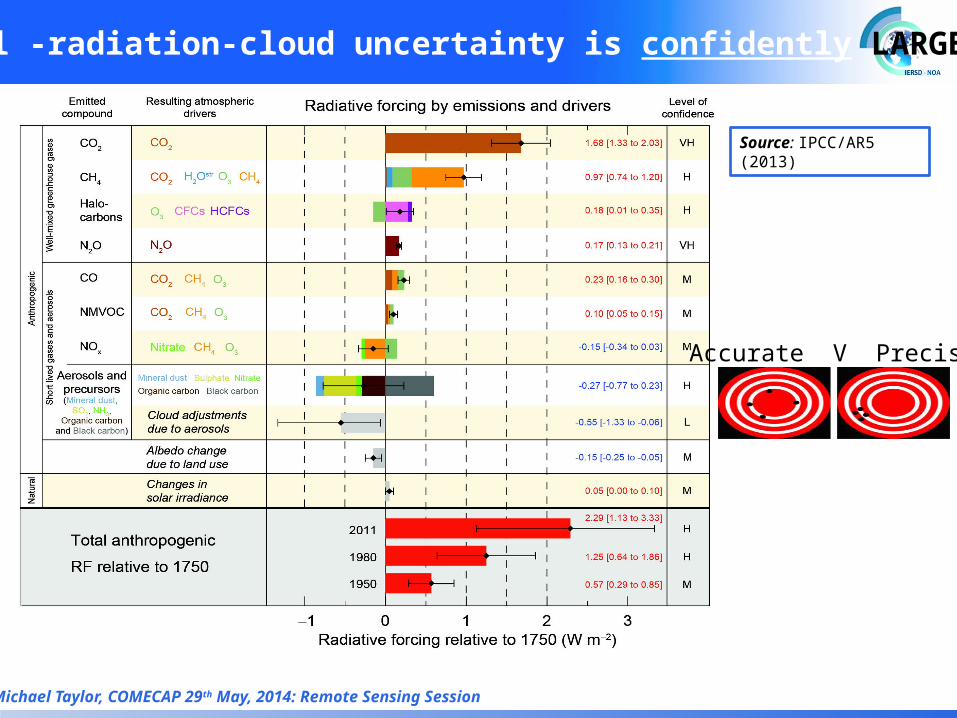
Aerosol -radiation-cloud uncertainty is confidently LARGE
Source: IPCC/AR5 (2013)
Michael Taylor, COMECAP 29th May, 2014: Remote Sensing Session
Accurate V Precise
Michael Taylor, COMECAP 29th May, 2014: Remote Sensing Session
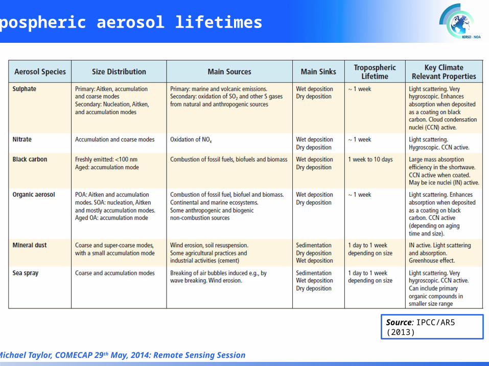
Tropospheric aerosol lifetimes
Source: IPCC/AR5 (2013)


![[REMOTE SENSING] 3-PM Remote Sensing](https://img.pdfslide.us/doc/110x75/61f2bbb282fa78206228d9e2/remote-sensing-3-pm-remote-sensing.jpg)

