Michael Plante - Federal Reserve Bank of Dallas ... · Michael Plante Federal Reserve Bank ... Given their cost and persistence, ... them out in the short-run by temporarily limiting

The Long-run Macroeconomic Impacts of Fuel Subsidies

Michael Plante

Federal Reserve Bank of Dallas Research Department Working Paper 1303 March 2013

The Long-run Macroeconomic Impacts

of Fuel Subsidies

Michael PlanteaaFederal Reserve Bank of Dallas

[email protected]∗

March 2013

Abstract

Many developing and emerging market countries have subsidies onfuel products. Using a small open economy model with a non-tradedsector I show how these subsidies impact the steady state levels ofmacroeconomic aggregates such as consumption, labor supply, and ag-gregate welfare. These subsidies can lead to crowding out of non-oilconsumption, inefficient inter-sectoral allocations of labor, and otherdistortions in macroeconomic variables. Across steady states aggregatewelfare is reduced by these subsidies. This result holds for a countrywith no oil production and for a net exporter of oil. The distortionsin relative prices introduced by the subsidy create most of the welfarelosses. How the subsidy is financed is of secondary importance. Ag-gregate welfare is significantly higher if the subsidies are replaced bylump-sum transfers of equal value.

Keywords: oil, fuel-price subsidies, developing countries, fiscal policyJEL Classifications: Q43, E62, H30, O23

∗This is a heavily revised chapter of my thesis that previously circulated under the title“The Long-run Macroeconomic Impacts of Fuel Subsidies in an Oil-importing DevelopingCountry.” For many useful comments and suggestions I give thanks to the editor, twoanonymous referees, Nathan Balke, Edward Buffie, Scott Davis, Michael Sposi, and MineYucel. Thanks also goes to seminar participants at the MEA 2012 meetings and theUSAEE 2012 meetings. Amy Jordan provided excellent research assistance. All mistakesremain my own. The views presented in this paper are mine alone and do not reflect theofficial views of the Federal Reserve Bank of Dallas or the Federal Reserve System as awhole.

1

1 Introduction

Subsidies on petroleum products are an important policy issue for manydeveloping and emerging market economies. One reason is the sheer costthese subsidies impose on the governments that provide them. Data from theInternational Energy Agency (IEA) and the International Monetary Fund(IMF) provide many examples for net oil importing countries where thesubsidies are on the order of 1 to 2 percent of GDP, sometimes higher. Fornet oil exporting countries the subsidies are often larger. Despite their costs,these subsidies are difficult to remove once in place and attempts to removethem, even partially, have often failed. This has been true even with thesignificant increase in oil prices seen over the last decade.1

Given their cost and persistence, it seems probable that these subsidieshave important macroeconomic implications. This paper asks three inter-related questions in regards to this. First, how do these subsides affectmacroeconomic variables and aggregate welfare in the long-run? Second,what role does the method of financing the subsidy play in those results?Finally, does the distinction between being a net importer or exporter of oilmatter?

To answer to these questions I construct a small open economy modelwith traded and non-traded sectors where households and firms use oil. Thegovernment subsidizes oil by selling it below its world price. The subsidyconsidered in this paper is a permanent (long-run) feature of the economy.As such it distorts the steady state and imposes a permanent financingconstraint on the government.2

Two variants of the model are considered. The first is an economy thathas no domestic production of oil. This variant is referred to as the netoil importing model. In this model the government finances the subsidythrough one of three tax instruments: a non-distorting lump-sum tax, a taxon labor income, or a tax on non-oil consumption. In the second variant,the net oil exporting model, the government has an endowment of oil thatis greater than domestic consumption of oil. In this case the governmentprovides the subsidy by simply selling part of its oil endowment below theworld price of oil.

1For more evidence please see Baig et al. (2007) and Coady et al. (2010).2Some governments do not distort domestic fuel prices in the long-run but do smooth

them out in the short-run by temporarily limiting the pass-through of a change in worldprices. Chile is one such example. Considering these policies requires looking at short-run dynamics and working with second-order approximations to the model. Given thedifferent nature of such short-run subsidies, this is left for future research.

1

For the net oil importer case the results show that the subsidy reducesaggregate welfare across steady states.3 For a subsidy that costs 1 percentof GDP the welfare losses are relatively minor but these costs increase sub-stantially for larger subsidies. Surprisingly, the method used to finance thesubsidy has relatively little impact on this result. The distortion in relativeprices introduced by the subsidy is responsible for the bulk of the welfarelosses. This is confirmed by considering the losses that would occur if thegovernment simply removed the subsidy and offset it with lump sum trans-fers of equal value. Aggregate welfare losses are about 20 times lower underthis policy than the one with the subsidy.

In the net oil exporter case the government does not need to rely onan explicit tax to finance the subsidy. Surprisingly, the different financingmethod available to net exporters does not significantly alter the aggregatewelfare results. This is due to the fact that the distortion in relative prices isthe main reason that aggregate welfare is lower. That feature of the subsidyis exactly the same whether the country is a net oil exporter or importer.

Underlying the welfare results are the actual changes in macroeconomicvariables that occur because of the subsidy. Regardless of how the subsidy isfinanced, it leads households and firms to over-consume oil products, drivesup wages in the economy, and increases production in the traded sector. Thesubsidy also distorts the relative price of non-tradables to tradeable goods.

The change in other macroeconomic variables, such as non-oil consump-tion, production in the non-traded sector, and labor supply depends uponthe tax instrument used to finance the subsidy. Essentially, households payfor the higher taxes required to finance the subsidy through some combi-nation of lower non-oil consumption and higher hours worked. The exactbreakdown depends upon which tax instrument is used because they distorthousehold behavior in different ways. Using labor or consumption taxes tofinance the subsidy usually leads to a crowding out of non-oil consumption.This in turn lowers production in the non-traded sector and leads to an inef-ficient allocation of labor across sectors as labor flows out of the non-tradedsector into the traded sector. All of these are important effects of a fuelsubsidy typically not discussed by policy makers when considering the prosand cons of the subsidy.

There is a large literature that focuses on oil and the macroeconomy.To my knowledge this is the first paper in that literature that looks at the

3Note these results do not provide any answers about how different groups withinthe economy are impacted, only how the economy as a whole is. It is quite possible thatdifferent groups may have higher or lower welfare depending upon how much of the subsidythey receive and how much of the tax burden they bear, amongst other things.

2

long-run macroeconomic impacts of fuel subsidies and the fiscal policy issuesassociated with them.4 Several IMF working papers, such as Coady et al.(2006) and Kpodar (2006), have considered the distributional impacts ofremoving fuel subsidies on household expenditure by using social accountingmatrix and input-output models. However, those models generally abstractfrom the fiscal policy aspect of the subsidy. As a consequence, removing asubsidy is unambiguously “bad” in those models because it means higherprices for all households. My model, which incorporates fiscal policy andgeneral equilibrium effects, suggests things may be more complicated. Whileremoving the subsidy forces households to pay higher fuel prices it alsoimplies lower taxes and reduced deadweight losses in the economy.

A related literature focuses on monetary policy responses to changes inthe price of food, another good often subsidized in developing countries.For example, Catao and Chang (2010) explore the role food prices playin determining what price index a central bank should stabilize in a smallopen economy. Anand and Prasad (2010) consider a similar question in atwo sector New Keynesian model where there is a flexible price “food” sectorand a “non-food” sector which has sticky prices. Agents who work in thefood sector are unable to smooth consumption over time due to a creditconstraint. Both of these show that under certain conditions a central bankmay want to stabilize headline inflation as opposed to the usual result ofstabilizing sticky-price inflation. Neither paper incorporates subsidies intotheir models.

The rest of the paper proceeds as follows. In the second section I moti-vate the paper by presenting some data on fuel subsidies. The third sectionintroduces the model economy for the net oil importer case. The resultsfor this case are presented in the fourth section. The fifth section presentsresults for the net oil exporter case. Section six shows results for sensitivityanalysis. Section seven concludes.

2 Empirical Motivation

This section presents some evidence on the prevalence and size of fuel sub-sidies, and energy subsidies more generally, between the years of 2000 to

4Aissa and Rebei (2012) considered optimal monetary policy in a two sector, closedeconomy New Keynesian model where the government stabilizes the price of one of thegoods in the short-run. However, the subsidy in Aissa and Rebei (2012) is a short-runphenomenon only and their analysis focuses on monetary policy, not fiscal policy.

3

2012.5 The main source of data on these subsidies comes from the IEA, theIMF, and several other international agencies. For this reason, I first discusshow these agencies define and measure energy subsidies. I then documentsome features of the data available from them and conclude by giving moredetail on the specifics of energy subsidies in three countries.

2.1 Defining Subsidies

The IEA focuses on subsidies that lower the price consumers pay for oilproducts, natural gas, coal, or electricity generated with one of those fuels.6

These subsidies tend to be the easiest to quantify and in terms of their sizeappear to be the most important for the time frame being considered. Theworking definitions of other institutions, such as the IMF, appear to be quitesimilar in practice so they are not discussed explicitly.

To identify and quantity the size of these subsidies the IEA follows Larsenand Shah (1992) and uses the price-gap approach. In this approach subsidiesare measured by calculating the gap between a domestic retail price and areference price which attempts to measure the true economic cost of theproduct being subsidized.

Estimates of subsidies calculated using the price-gap approach can re-flect both opportunity costs and explicit costs. For a country with no oilproduction the subsidy is an explicit cost, one typically paid for by the gov-ernment. For a net oil exporter the subsidy is typically an opportunity costbecause in many cases the government simply sells domestically producedoil below its world price. The estimate then simply reflects the foregonerevenue from not selling the oil at its economic cost. For a net oil importerwith some domestic production the estimate is both an explicit cost and anopportunity cost.

2.2 IEA Data on Fuel Subsidies

Currently the most comprehensive, publicly available data set on energysubsidies is from the IEA. These are annual estimates, in billions of dollars,on the size of consumer subsidies on oil products, natural gas, coal, andelectricity generated using fossil fuels in a total of 37 countries. The databegin in 2007 and end in 2011. Here I touch upon some of the more relevant

5Data on fuel subsidies in the 1980s and 1990s was sparser. For that reason this sectionfocuses on the time frame mentioned.

6For the exact definition please refer to IEA (2010) or IEA (2011).

4

features of the data for this paper. Those interested in more detail shouldrefer to IEA (2010) or IEA (2011).

For the five years considered, the total value of all energy subsidies acrossall 37 countries was $342B, $555B, $311B, $412B and $523B, respectively.Changes in any given year were to a large extent driven by changes in theprice of oil. Subsidies on oil products made up the largest share of the total,on average a little under 50 percent. Out of the 37 countries identified ashaving a subsidy, 34 had subsidies on oil products, of which 21 were net oilexporters and 13 were net oil importers.7

One way to rank which country has large subsidies is by considering thedollar value of the subsidies in place. If one ranks countries by this metricthen the biggest subsidizers are generally either net oil importers which havelarge populations, such as China or India, or important net oil exporters suchas Iran or Saudi Arabia. For illustrative purposes the top panel in table 1ranks the top five net oil importing and exporting countries using the 2011data as an example.

For the issues considered in this paper a better measure to consider is thesize of the subsidies in relation to an economy’s GDP. This provides someinformation on how much of a cost the subsidies impose on the governmentand the economy in question. The bottom panel of table 1 reconsiders thetop five net oil importers and exporters according to this metric using the2011 data. While absolute size of the subsidy does sometimes predict alarge subsidy in relation to the domestic economy, this is not always thecase. For example, China’s fuel subsidies were huge in dollar terms but inrelation to its economy they were fairly small, coming in at a quarter of apercent of GDP. On the other hand, Sri Lanka’s subsidies were fairly smallin dollar terms, less than a billion dollars, but relatively large in terms ofthe economy.

Measuring subsidies in relation to a country’s GDP highlights an im-portant dichotomy between many net oil exporters and importers. Figure1 shows this graphically by plotting a histogram with countries categorizedby their subsidy-GDP ratio. The data from 2011 is used as an example. Fornet oil importers every country was between 0 and 2 percent of GDP, exceptfor Egypt. For net oil exporters there was a cluster of countries between 0and 3 percent of GDP. But there was also an additional cluster of 6 countrieswhich had subsidies between 5 to 9 percent of GDP, as well as an outlier

7Countries are defined as net oil exporters or net oil importers using data on annual oilsupply and consumption from the Energy Information Administration (EIA) InternationalEnergy Statistics.

5

with subsidies well over 10 percent of GDP. The cluster of 6 countries wereall OPEC countries, while the outlier was Iraq.

There are two reasons behind this tendency for subsidies to be largerin net oil exporting countries. First, many net oil exporters tend to sub-sidize a wider range of products than net oil importers. In many cases alldomestically consumed products are subsidized. Holding all else equal, thisenlarges the base being subsidized and increases the cost of the subsidy. Asecond factor is that net oil exporters often have significantly lower retailprices compared to net oil importing countries with subsidies. Taken to-gether these two factors tend to increase the size of the subsidies found innet oil exporters.

For illustrative purposes table 1 and figure 1 used the data from 2011.For those interested in other years or other countries, the data for all 34countries and 5 years can be found in a table C-4 in the appendix.

2.3 Considering Natural Gas and Electricity Subsidies

While attention often falls on fuel subsidies, both natural gas and electricitysubsidies are also important in size. According to the IEA data, subsidies onelectricity produced using fossil fuels and subsidies on natural gas averagedclose to 27 percent and 23 percent of the total share, respectively, over the 5years considered.8 Natural gas subsidies were identified in 9 countries whichwere net importers of natural gas and 10 which were net exporters of naturalgas. A total of 34 countries were identified as having electricity subsidies.

From an individual country’s perspective, natural gas subsidies couldoften be modeled in a similar fashion to fuel subsidies. For example, considerthe case of a net importer of natural gas with a subsidy. The governmentpurchases natural gas at a price determined in a market (often linked tooil prices), sells it below cost, and must finance this through some form oftaxation. If the country is a net exporter of natural gas then the governmentcan finance the subsidy by selling domestically produced natural gas belowits market price, in which case the subsidy is an opportunity cost.

In many cases electricity subsidies can also be treated in a similar man-ner. While electricity itself is often not traded between countries, it is inmany cases generated using imported inputs such as oil products and nat-ural gas. In this case an electricity subsidy is basically an indirect subsidyon the consumption of the imported fuel. For a net importer of the input,the end result is essentially the same for the government in question, and

8Consumer subsidies on coal were negligible in size and are henceforth ignored.

6

likewise for the government of a net exporting country.In what follows, I continue to refer generically to fuel subsidies. However,

in many cases this could be interchanged with natural gas subsidies or elec-tricity subsidies and the general results should carry over for those cases.Two examples are provided in section 2.5 which highlight the similaritiesbetween the different types of subsidies.

2.4 Additional Sources of Data

Additional sources allow one to expand the IEA data by including morecountries and considering years prior to 2007. For some countries, addi-tional data on the costs of their subsidies is also available. Using the largerset of sources, I identified another 21 countries that had a fuel subsidy atsome point in time between 2000 to 2012.9 For subsidies on electricity pro-duced using fossil fuels an additional 15 countries were identified. No othercountries were found to have natural gas subsidies besides those listed in theIEA data.

Unfortunately, it is not possible to expand the quantitative data fromthe IEA for all of the additional countries or years. There are some countrieswith fairly detailed data on the costs of the subsidies, but in many cases thesource documents mention the existence of a subsidy but provide no dataon its cost. Consequently, there are too many gaps to construct a compre-hensive estimate of the costs across countries and across time. However, atable in the appendix shows the subsidy costs, as a share of GDP, for thecountries and years in which that data was available.

2.5 Country Experiences

Indonesia, Ukraine, and Lebanon provide useful examples of how differenttypes of energy subsidies operate and what their costs are to the govern-ments that choose to put them in place. Indonesia subsidizes a wide rangeof oil products; Ukraine subsidizes household consumption of natural gas;Lebanon subsidizes electricity, almost all of which is produced using im-ported oil products.

9A list of these countries and the sources used to identify them can be found in theappendix.

7

Fuel Subsidies in Indonesia10

Indonesia has had experience with subsidies on oil products as both anet exporter and net importer of oil.11 Indonesia’s national oil company,Pertamina, is heavily involved in the production, importation, and distri-bution of oil products in the country. Domestic retail prices are set by thegovernment on an ad hoc basis and subsidies have been in place since thelate 1960s. The subsidies take the form of explicit underpricing of the prod-ucts compared to their actual cost. Pertamina is compensated for this andthe costs of the subsidy are reflected in the Indonesian budget.

Most products are currently subsidized, except for some premium gradesof gasoline. Using IMF data it is possible to get estimates on the costs ofthese subsidies, as a percent of GDP, from 2000 to 2012. These are listed inthe second column of table 2. The subsidies have been more than 1 percentof GDP each year, and in many cases well above that.

Electricity Subsidies in Lebanon12

Lebanon provides a very good example of a country with subsidies onelectricity produced using an imported fossil fuel. On average, about 94percent of its electricity was generated using imported oil products between2000 - 2010.

The state-run electric utility company, Electricite du Liban, has receiveddirect transfers from the government every year since 1984. These transfersare often used to cover the gap between the cost of the imported fuel andthe revenues the company generates from underpriced electricity. Electric-ity tariffs have been frozen since 1996 and are priced for $21 a barrel oil,according to an estimate in IMF (2012).

Data from the World Bank and the IMF allow one to calculate the costof the subsidy, as a percent of GDP, from 1984 up to 2012. The third columnof table 2 shows how the costs have varied from 2000 until 2012. The subsidycost about 1 percent of GDP in the early part of the decade, but since 2005has been roughly 3 percent of GDP or higher. The 2011 and 2012 estimatesfrom the IMF come in at 4.5 percent of GDP. Projections up until 2016currently put the cost over 4 percent of GDP each year.

Natural Gas Subsidies in Ukraine13

Ukraine is a net importer of natural gas with some domestic production.A state-owned company, Naftogaz, is heavily involved in the production,

10Sources: EIA (2011), EIA (2012), Clements et al. (2003), IISD (2012a), IISD (2012b)OECD (2010).

11Indonesia became a net importer of oil and oil products in 2004.12Sources: EIA (2012), IMF (2012), World Bank (2008).13Sources: EIA (2012), IEA (2012), Mitra and Atoyan (2012), Petri et al. (2002).

8

importation, and distribution of natural gas in the country. The gas isconsumed by both industry and households and is also used to generateelectricity. Household consumption of natural gas is heavily subsidized, withtariffs well below import cost. Industry usage is not subsidized and firmspay a price that reflects import costs.

Measuring the cost of natural gas subsidies in Ukraine is difficult asNaftogaz’s activities are quasi-fiscal in nature and the cost of the subsidieshas not always been fully reflected in the government’s budget. However,the IEA dataset provides a dollar amount for these subsidies for the yearsfrom 2007 to 2011. For these five years the subsidies totaled $4.8B, $8.3B,$5.3B, $5.2B, and $6.7B, respectively. As a share of GDP this translates to3.4 percent, 4.6 percent, 4.5 percent, 3.8 percent, and 4 percent.

3 The Model for the Net Oil Importer

I consider a small open economy that produces a composite traded good anda non-traded good. Both goods are produced using labor and oil and onesector may be more or less oil-intensive than the other. The traded goodis the numeraire and for convenience its price is fixed at unity. The tradedgood is either consumed by households or used to purchase oil from the restof the world. The economy is small in that it has no effect on the worldprice of the traded good or the world price of oil.

The notation used in the exposition is as follows. The time derivativeof the variable X is X, X is the steady state value of X, and X is thelog-differential of X, i.e. X = dX/X.

3.1 Households

Household activity is controlled by an infinitely-lived representative agentwho derives disutility from working and utility from the consumption oftraded and non-traded goods, as well as fuel products.

Total labor supply is denoted as L = LT +Ln where LT and Ln are laborsupplied to the traded and non-traded sector, respectively. Consumption ofthe traded, non-traded, and oil goods are denoted as CT , Cn, and Oh,respectively. The agent has access to a real domestic bond, denoted asb. The representative agent assumption implies this will be in net zerosupply in equilibrium. Households do not have access to international capitalmarkets.14

14Currency substitution is a feature of many of the countries that have fuel subsidies.

9

Preferences are given by

U =

∫ ∞0

[C(CT , Cn, Oh)1−

1τ

1− 1τ

− κV (L)

]e−ρsds, (1)

where

C(CT , Cn, Oh) =

(CT

σc−1σc + a1C

nσc−1σc + a2O

hσc−1σc

)( σcσc−1

),

V (L) =L1+ 1

µ

1 + 1µ

.

The parameter τ is the elasticity of intertemporal substitution; µ is theFrisch elasticity of labor supply; σc is the elasticity of substitution betweenthe consumption goods, ρ is the time-preference rate; a1, a2, and κ areconstants.

The agent maximizes equation(1) subject to the flow constraint

b = (1−τ l)(WnLn +W TLT

)+Tr+rb−(1+τ c)

(CT + PnCn

)−P sOh−T.

(2)Income from labor is given by W TLT + WnLn where W T and Wn are

the wages in the traded and non-traded sectors. This income is taxed ata rate of τ l. Interest income on savings is given by rb and will be zeroin equilibrium. Lump-sum transfers from the government are given by Tr.Expenditure on non-oil consumption is given by CT +PnCn where Pn is therelative price of the non-traded good to the traded good. This consumptionis taxed at a rate of τ c. Lump-sum taxes are given by T . Expenditure onoil consumption is given by P sOh, where P s is the subsidized price of fuelproducts. Denoting P o as the world price of oil, the assumption is thatP s ≤ P o.

The first order conditions for the agent’s problem can be written as15

UnUT

= Pn, (3)

UoUT

=P s

1 + τ c, (4)

κVlUT

=1− τ l

1 + τ cW T , (5)

To simplify the exposition I abstract from this possibility in the model. For some resultswith a model that incorporates this feature please see the previous version of this paper.

15Please see the appendix for the exact forms of the first order conditions

10

Wn = W T , (6)

λ

λ= ρ− r, (7)

where λ is the multiplier on the flow constraint and Un, UT , and Uo are thederivatives of the utility function with respect to the non-traded, the traded,and the oil consumption good.

Equation (3) sets the marginal rate of substitution between traded andnon-traded consumption goods equal to their relative price while equation(4) does the same for the oil consumption good. Equation (5) equates themarginal dis-utility of working an additional hour equal to the marginalbenefit of doing so. Equation (6) states that wages are equivalent across thetraded and non-traded sectors. This is because of the assumption that laboris mobile across sectors.

The subsidy directly distorts the first order conditions through the rel-ative price term, P s, in equation (4). There are additional distortions ifconsumption taxes or labor taxes are used to finance the subsidy, or if thesubsidy impacts wages or the relative price of the non-traded good. Allof these distortions will impact household consumption and labor supplydecisions.

3.2 Production

Production in the two sectors is done by representative firms operating underperfect competition. The firms have a CES technology of the form

Qi(Li, Oi) =

[(AiLi

)σi−1

σi + bi(Oi)σi−1

σi

] σiσi−1

, (8)

where i = T, n for the traded and non-traded sectors, Ai and bi are constants,Oi is oil demanded by sector i, and σi is the elasticity of substitution betweenvalue-added (here labor) and oil.

The first order conditions for the firms are given by

QTl = W T , (9)

QTo = P s, (10)

Qnl =Wn

Pn, (11)

Qno =P s

Pn, (12)

11

where Qil and Qio are the derivatives of the production functions with respectto labor and oil. The first order conditions equate the marginal products ofeach input with its respective marginal cost. The relative price term appearsin the first order conditions for the non-traded sector due to the choice ofthe numeraire.

Cost functionsThe functional form for the production function implies that unit costs

for each firm, denominated in terms of the traded good, are

Φi(W i, P s) =

(W i

Ai

)1−σi+ bi

σi (P s)1−σi

11−σi

(13)

for i = T, n. Furthermore, the relative price of the non-traded good is givenby

Pn =Φn

ΦT. (14)

One can derive two additional and very useful conditions using these costfunctions and the equation for Pn.

Facing a constant world price for its output and under the assumptionsmade regarding production, the real unit cost in the traded sector, ΦT , isequal to 1. Using this condition, one can immediately show that wages in thetraded sector will increase if P s is lowered in the long-run. More specifically,for small changes in P s the change in the wage is given by

W T = −αTo

αTlP s, (15)

where αTo and αTl are the cost shares of oil and labor in the traded sector.Intuitively, lower energy costs would allow firms in the traded sector

to sell their output below the world price of the traded good. This wouldincrease demand for their good, and to meet this demand the firm wouldneed to use more labor. The only way to attract this labor is for wages toincrease. In the new long-run equilibrium the firm increases its production,and its demand for labor, until the point where its cost of producing anadditional unit of output would once again equal the world price of thetraded good. Equation (15) provides the exact change in wages required toensure that this condition holds. The more oil-intensive the traded sector isthe greater the increase in wages will be.

The household’s first order condition in equation (6) implies that thechange in W T spills over into the non-traded sector. The increase in W T ,

12

therefore, acts as a negative cost shock for the non-traded sector. Holdingall else equal, this would drive up Pn. But, the non-traded sector also faceslower energy costs because it benefits from the subsidy. In the end whichone of these forces wins out depends upon how oil-intensive the non-tradedsector is. For a small change in P s the change in Pn is given by

Pn =

(αno −

αnl αTo

αTl

)P s, (16)

where αno and αnl are the cost shares of oil and labor in the non-traded sector.If the non-traded sector is oil-intensive enough then reductions in P s reducecosts so much that Pn declines. Otherwise the increase in wages drives upcosts and Pn increases.

3.3 The Government

The government earns revenue from lump-sum taxes, taxing labor incomeand taxing the consumption of non-oil consumption goods.16 On the ex-penditure side, the government provides a subsidy on fuel products andlump-sum transfers to households. The government purchases oil at theworld price of P o and then sells it at the subsidized price P s, with P s ≤ P o.While simple in nature, this assumption regarding the subsidy captures theimportant fact that domestic prices are lower than world prices and that thesubsidy must be financed by the government somehow.

In the steady state the government budget constraint reads

T + τ l(WT LT + WnLn

)+ τ c

(CT + PnCn

)= T r+

(P o − P s

) (Oh + OT + On

). (17)

3.4 Market Clearing and the Current Account

Market clearing in the non-traded sector implies

Cn = Qn. (18)

In the bond market the equilibrium condition is

b = 0, (19)

both in and out of the steady state.In the long-run trade balances so

QT = CT + P o(Oh + OT + On

). (20)

16Consumption and income taxes were chosen on the basis of IMF country reports whichshowed that these two forms of taxation tend to be important sources of revenue for manydeveloping countries. This is particularly true of taxes on goods and services.

13

3.5 Calibration

The model is calibrated to an initial steady state where there are no subsi-dies. Parameters and variables are calibrated to match features of a typicaldeveloping country that has had experience with fuel subsidies, such asBangladesh, Sri Lanka, or Indonesia. Units are chosen so that real GDP isequal to 1, as are P o and Pn. Lump-sum transfers, Tr, are set to 0. Totalhours worked is set to 1/3. Table 3 lists the calibration of the model’s otherparameters and variables, along with short comments on the sources usedin the calibration. Greater detail regarding the sources can be found in theappendix. The calibration of several elasticities and the amount of oil usedby firms is discussed in more detail below.

• Elasticities of substitution (σc, σn, σT ) - These parameters pin down theprice-elasticity of demand for oil products. A survey done in Grahamand Glaister (2002) shows that long-run elasticities for many countriestend to cluster around -.6 to -1 and that these are larger than short-run elasticities. The baseline calibration is in line with these findings.An alternative calibration of .25, more consistent with short-run priceelasticities, is also considered.

• Frisch elasticity of labor supply (µ) - This parameter controls howresponsive labor supply is to changes in wages, with larger values im-plying a greater responsiveness. Even for developed countries thereis significant uncertainty surrounding this parameter. Reichling andWhalen (2012) provides a useful summary of the findings. Micro esti-mates tend to be smaller than macro estimates, often between 0 and1, as an individual’s hours worked tends to be unresponsive to changesin wages. Macro estimates are often between 2 and 4, reflecting thefact that in aggregate data this elasticity is capturing changes in boththe intensive and extensive margins on how much people work. Thebaseline calibration sets µ equal to 1, but an alternative calibration of3 is also considered.

• Firm demand for oil - Input-output tables for 11 developing countriesare available from the OECD STAN database. These tables providedata on spending by firms on “Coke, refined petroleum products, andnuclear fuel.” This provides the best estimate on total firm spending onoil products. In theory, one would like to have an estimate for spendingonly on “refined petroleum products” but unfortunately that data isnot available. The average value was close to 5 percent of GDP for allfirms. About 40 percent of that was due to firms in the traded sector

14

(defined as agriculture, mining, and manufacturing).

4 Results

Numerical solutions are calculated for how the model’s variables change con-ditional on the method of financing the subsidy and the size of the subsidy,in relation to initial GDP. I consider subsidy costs that range from 1 to 4percent of GDP. For each level of the subsidy, one of the tax instrumentsadjusts to clear the government budget constraint. Labor taxes, consump-tion taxes, or lump-sum taxes are each considered in turn. With three fiscalinstruments this results in a total of 12 cases considered.

The analysis of the results focuses on how the model’s variables changeacross steady states and on how aggregate welfare is impacted by the changesin those variables. Changes in the variables are calculated as percent changesacross steady states, where the initial steady state (with no subsidy) is thepoint of reference.

If Xo and X1 are the steady state values of variable X in the originaland the new steady state, respectively, then the change in aggregate welfareacross steady states is given by

1

ρ

C

(CTo , C

no , O

ho

)1− 1τ

1− 1τ

− κV (Lo)

−[C(CT1 , C

n1 , O

h1 )1−

1τ

1− 1τ

− κV (L1)

] .However, looking at the change in aggregate welfare across steady states isnot very informative since utility is ordinal. To make the comparisons moreconcrete, I solve for how much aggregate consumption in the initial steadystate would need to be increased or decreased, in percentage points, to makewelfare equal across the two steady states. Mathematically I solve for ω inthe following equation,[ωC(CTo , C

no , O

ho )]1− 1

τ

1− 1τ

− κV (Lo)

−[C(CT1 , C

n1 , O

h1 )]1− 1

τ

1− 1τ

− κV (L1)

= 0.

(21)In general ω will be non-zero as welfare will be higher or lower across steadystates. The welfare losses are calculated as

Wl = 100 ∗ (1− ω) . (22)

15

One way to interpret Wl is as follows. If Wl is positive then aggregate welfareis higher in the initial steady state. Intuitively, aggregate consumption wouldneed to be lowered by Wl percent to match the lower utility in the new steadystate. Alternatively, Wl tells one how much aggregate consumption wouldneed to be increased to make the agent as well off in the new steady stateas in the initial steady state.

When households and firms receive the subsidy, the solutions combinethe effects brought about by changes in the relative price that householdsface for Oh and changes in the relative price that firms face for OT and On.It is instructive to consider each of these channels separately. To do so Ifirst solve for a case where the household pays the subsidized price but thefirm pays the world price of oil. Second, the case where the firm receives thesubsidy but households do not is considered. Finally, I present the resultsunder the situation where both households and firms receive the subsidy.

4.1 Households Receive the Subsidy

In many countries, households are often specifically targeted as the benefi-ciaries of the subsidy. This is particularly true for certain oil products aswell as electricity and natural gas, which are harder to divert from theirintended recipients. For this reason, it is interesting to first consider theresults under the assumption that only households receive the subsidy. Do-ing so only requires assuming firms pay the prevailing price for oil products,P o, and the government only needs to raise revenue for under-pricing fuelproducts to households. All other aspects of the model remain the same.

The top panel in table 4 presents the results for aggregate welfare. Eachrow is for a different subsidy cost while columns two through four record theresults for the different tax instruments. The numbers in each entry tell ushow much aggregate consumption in the initial steady state would need tobe decreased to get welfare equal across steady states. For example, if thesubsidy costs 4 percent of GDP and is financed by a consumption tax Wl isequal to 1.4. This means that aggregate consumption in the initial steadystate would need to be 1.4 percent smaller to match the (lower) aggregatewelfare of the new steady state.

Regarding the subsidy’s impact on aggregate welfare, the numbers inthis table are all positive, so aggregate welfare is always lower with thesubsidies. In consumption-equivalent terms the welfare costs are fairly smallfor subsidies on the order of one percent of GDP, coming in at little over atenth of a percent of aggregate consumption. However, the losses steadilyincrease as the subsidy reaches higher levels and Wl is well over 1 percent

16

by the time the subsidy reaches 4 percent of GDP.Interestingly, the method of financing the subsidy is of secondary impor-

tance to the subsidy itself in terms of the welfare losses. There are differencesbetween the different tax instruments but they are fairly small. In general,lump-sum taxes or labor taxes are slightly preferred to financing the subsidythrough a consumption tax.

Underlying the welfare results are the actual changes in the variablesacross steady states. The top panel in table 5 shows these results. Eachcolumn is for a different tax instrument. For brevity’s sake the results areshown only for the case where the subsidy costs 1 percent of GDP. Largersubsidies would increase the size of the changes that occur, so one shouldview the quantitative results in the table as a sort of lower bound. Notealso that if one wanted to consider the implications of going from the steadystate with the subsidy to the steady state without the subsidy, one needsonly flip the signs on the results found in the table.

For the baseline calibration a subsidy of 1 percent of GDP leads to areduction in the subsidized price of fuel by about 26 percent.17 Regardless ofhow the subsidy is financed, lower fuel prices induce households to consumeroughly 25 percent more fuel.

How the other variables change across steady states depends upon themethod of taxation used. Essentially, households pay for the increased taxesby consuming less non-oil goods, working more, or both. The exact break-down depends upon which tax instrument is used because different tax in-struments distort household behavior in different ways.

Lump-sum taxes reduce disposable income but do not otherwise changethe effective prices that households face and for this reason they make auseful baseline case. When the subsidy is financed by lump-sum taxes,households both consume less and work more. Consumption of non-oil goodsdeclines by half a percentage point while hours worked increases by abouthalf a percent.

By comparison, labor taxes reduce the incentive to work so hours workedincrease less. However, as a consequence, households cut back consumptionof non-oil goods by a greater amount. Consumption taxes not only reducethe incentive to work but also further distort the relative price of the con-sumption goods. Compared with lump-sum taxes, hours worked increase bymuch less, consumption of oil products rises more, and consumption of other

17The change in P s is a mainly a function of the specified subsidy cost and how big thebase being subsidized is. If a great deal of oil is consumed by the economy, then smallchanges in P s are sufficient to reach a specified level of subsidy cost and vice-versa.

17

goods falls by a greater amount. The fact that the consumption tax intro-duces two distortions appears to be the reason it generates slightly higherwelfare losses than the other two forms of taxation.

Although firms do not benefit from the subsidy, production variablesare impacted indirectly. Reduced demand for the non-traded good causesproduction in that sector to decline, which lowers that sector’s demandfor labor and oil. In the long-run this labor flows into the traded sector.Despite labor re-allocating across sectors, wages remain unchanged as thetraded-sector faces a constant real unit cost and a constant price P o for oilinputs. What does happen is that the traded sector expands production byincreasing its use of oil and labor proportionally.18

4.2 Firms Receive the Subsidy

Now suppose that firms pay the reduced price of P s for oil while householdscontinue to pay the world price P o. The middle panel in table 4 shows thewelfare results for this case. The format of the table is exactly the same asbefore. Each entry in the table is positive, showing that aggregate welfareis reduced by the subsidy. The losses are fairly small for subsidies on theorder of one to two percent of GDP but start growing as the subsidy reacheshigher levels. The choice of the tax instrument is again essentially irrelevantfor the results.

The middle panel of table 5 shows how the variables change across steadystates. With lower energy prices, production expands in the traded sectorwhich brings about higher wages and greater labor usage in that sector. Theintuition behind these results is exactly as explained in section 3.2.

For the non-traded sector, things are a little more complicated. Asexplained in section 3.2 the higher wages drive up costs in this sector butthe subsidy lowers costs. For the baseline calibration, the non-traded sectoris more oil-intensive than the traded sector. The end result is that lowerenergy costs drive down unit costs enough to override the increases causedby higher wages in the economy. As a result, there is a small decline in therelative price of the non-traded good to the traded good. In response to thisreduction in Pn households are induced to consume more of the non-tradedgood leading output to expand in that sector as well.

While households do not directly receive the subsidy they do have to payhigher taxes. Which tax instrument is used to pay for the subsidy has some

18Demand for the two inputs increases proportionally because the firm faces a constantratio of input prices. This can be seen by combining the first order conditions for laborand oil in the traded sector, equations (9) and (10).

18

implications for how consumption and hours worked respond. The decreasein Pn leads to increased consumption of the non-traded good regardless ofthe tax instrument used. However, when labor taxes or consumption taxesare used, consumption of the traded good gets crowded out. The consump-tion tax induces households to substitute away from the taxed goods intooil. Consumption and labor taxes also reduce the overall increase in hoursworked by households compared to the lump-sum case.

Comparing the top and middle panels of table 4 shows that the welfarelosses are lower when firms receive the subsidy than when households receiveit. This is driven to some extent by the fact that the subsidies are beingmeasured by their size in relation to GDP. The baseline calibration has firmsusing more oil than households, so a smaller drop in P s is needed to reach agiven subsidy cost. This can be confirmed by comparing how P s changes inthe two cases using table 5. An alternate method would be to calculate thewelfare costs as a function of P s instead of the subsidy cost. Figure 2 plotsthe welfare losses as a function of P s for the three cases considered. Thedashed line is for the case where households receive the subsidy, the solidline for the case where firms receive the subsidy, and the dashed-dotted linefor the case where both receive the subsidy. This figure shows that for agiven reduction in P s, the losses are larger in cases with a bigger base beingsubsidized.

4.3 Households and Firms Receive the Subsidy

The bottom panel of table 4 records the welfare losses under the scenariowhere both households and firms receive the subsidy. In general the resultsare similar to the previous two cases. Comparing the three panels showsthat the losses are smaller in this case than in the other two cases. This isexplained by the fact that for a given subsidy cost the reduction in P s islowest in this case as the base being subsidized is the largest.

All of the movements in the variables are now combinations of the resultsfor the two previous cases. Households face a lower relative price for the oilgood and a slightly lower relative price for the non-traded good (comparedto the traded good). Households increase their consumption of fuel productsand reduce their consumption of traded goods. With Pn lower, consumptionof the traded good falls relatively more than the non-traded good. Bothlabor and consumption taxes reduce hours worked and consumption of non-oil products relative to the lump-sum case. Likewise, consumption taxesdrive up consumption of oil products at the expense of non-oil consumptioncompared to the lump-sum and labor tax case.

19

4.4 Transfers vs. Subsidies

Aggregate welfare is impacted by both the subsidy and the taxes necessary tofinance the subsidy. One result shown in table 4 is that only minor differencesare found for the change in aggregate welfare regardless of whether lump-sumtaxes, labor taxes, or consumption taxes are used to finance the subsidy. Onehypothesis for why this is the case is that the distortions in relative pricesintroduced by the subsidy are the main reasons that aggregate welfare islower and not because of changes in T , τ l, or τ c.

To consider whether this might be the case I ask what the implicationswould be on aggregate welfare if instead of increasing subsidies by a certainpercent of GDP the government increased lump-sum transfers by the sameamount. This would require changing τ l or τ c by a similar amount to payfor the increased government spending on Tr but would keep P s equal tothe world price of oil.

The specific experiment considers transfers on the order of 1 to 4 percentof initial GDP. These are financed with either labor or consumption taxes.Table 6 compares the aggregate welfare losses between increased transfersand the subsidy. For brevity’s sake only the results from the case wherehouseholds and firms receive the subsidy are presented. The results arestark: the losses under the subsidy are about 20 to 25 times greater thanunder a system of transfers. While the increased taxation required on anaggregate level is similar in both cases the distorted relative price signifi-cantly increases welfare losses under the subsidy. Similar results are seen inthe cases where only households or firms benefit from the subsidy.

This result might be of more than just theoretical importance. In gen-eral, it has been quite difficult for countries to remove fuel subsidies oncethey are in place. To increase the likelihood of a successful reform the IMFhas often suggested their removal be offset with increased transfers. Gener-ally it is argued that these transfers can be better targeted to the needy andare often less costly than the fuel subsidies they replace. The results in thispaper offer an additional reason for considering this option: giving peoplemoney and allowing them to spend it where they want is significantly moreefficient than inducing them to consume more fuel products by artificiallylowering fuel prices.

5 The Case of a Net Exporter

A large number of net oil exporters also subsidize fuel products. An impor-tant reason for considering the case of net oil exporters separately is that

20

they have an additional financing method available to them. The govern-ments of these countries can simply sell domestically produced oil belowits world price. This creates an opportunity cost for the government butnegates the need to raise taxes to finance the subsidy.

To address whether this significantly alters the previous results aboutaggregate welfare this section modifies the baseline model by assuming theeconomy has an endowment of oil large enough to make it a net exporterof oil. The punchline of the work is that the results are surprisingly similarto the case of the net oil importer. The reason for this is that whetherone is considering a net oil exporter or importer the subsidy distorts therelative price of fuel products and it is that distortion which drives most ofthe welfare results, not the method of financing the subsidy.

5.1 Households and Firms

No changes are made to the assumptions regarding household and firm be-havior. Preferences and the budget constraint of the household are assumedto be equivalent for the net oil importer and exporter. Technology in thetraded and non-traded sectors is also the same.

5.2 The Government

The major change to the model comes on the government side. In many netexporting countries the government is heavily involved in the productionof oil. In line with this, I assume the government now has access to anendowment of oil, Qo. I assume there is zero cost associated with the supplyof oil.19 The government earns revenue from selling oil domestically tohouseholds and firms at a subsidized price of P s and exports the remainingsupply at the world price, P o. All revenue from the sales of oil, whetherfrom exports or domestic sales, is funneled to the economy through a lump-sum transfer. For simplicity I assume the government does not levy taxes oneither labor income or consumption nor does it spend the money on anythingbesides the transfer. Under those assumptions the steady state governmentbudget constraint reads

P o(Qo − Oh − OT − On

)+ P s

(Oh + OT + On

)= T r. (23)

19This assumption potentially inflates the revenue the government receives from the saleof oil. However, I also considered a case where there was a fixed cost per unit of oil. Theresults were not significantly different.

21

There is a subtle point in the budget constraint worthwhile pointing out.If the net oil exporter has no subsidies in place, then government revenueis maximized at P oQo. With a subsidy in place, government revenue isreduced below this amount. But this automatically means lower transfersto the economy. In a very real sense, the subsidy is actually being financedby a reduction in lump-sum transfers.

5.3 Market Clearing and the Current Account

Market clearing in the non-traded sector and the bond market are equivalentfor the net oil importer and exporter.

The current account equation, however, is different. In the steady statethe current account for the net oil exporter reads

QT + P oQo = CT + P o(Oh + OT + On

). (24)

Essentially, the net oil exporter has extra oil and uses that to trade forCT whereas the net oil importer produces extra QT and trades that for oil.

5.4 Calibration

The model is calibrated to an initial steady state where there are no subsi-dies. Where possible the calibration found in table 3 is used for the modelof the net oil exporter as this facilitates comparison between this case andthe net oil importer case. The deep parameters, given by ρ, τ , σc, σT , σn,and µ are the same across models. Consumption expenditure shares andfirm use of oil as a percent of GDP are also calibrated to the same startingvalues.

I calibrate Qo as a proportion of total domestic consumption of oil. Toguide the calibration I used EIA data on “Total Oil Supply” and “Total OilConsumption” for Ecuador, a net exporter with large fuel subsidies. Forthat country, total oil supply was on average about 2.4 times the size oftotal oil consumption between 2007 and 2011 (the years for which data isavailable on subsidies in the country).

5.5 Results

Numerical solutions are calculated for how aggregate welfare varies acrosssteady states, depending upon the size of the subsidy as a fraction of initialGDP. This is the same procedure that was done for the net oil importer.

22

Table 7 presents the welfare results.20 For brevity’s sake only the resultsfor the case where households and firms receive the subsidy are presented.The second column shows the welfare costs for varying levels of the subsidycompared to the baseline case where there are no subsidies. While themethod of finance is quite different from what occurs in the net importermodel, the results are surprisingly similar. For subsidies of small size, thewelfare costs tend to be small but they become increasingly large as thesubsidies increase in cost.

This result may be unexpected. But it is in line with the intuition for theresults in table 6 that the method of finance was of secondary importance fora net oil importer. The biggest driver of the welfare losses is the distortionin relative prices that occurs with the subsidies, not the tax instrument usedto finance it. This distortion is a feature of the subsidy whether the countryis a net oil exporter or importer. Consequently the aggregate welfare resultsare similar in both cases.

6 Sensitivity Analysis

As a robustness check sensitivity analysis is performed on several of themodel’s parameters and variables. For brevity’s sake only the results forthe net oil importing country where both households and firms receive thesubsidy are presented.21

6.1 Low Price Elasticities

In the baseline calibration the elasticities of substitution for oil products areset at a level consistent with long-run price elasticities. However, there issome variation in the estimates of long-run elasticities and short-run elastic-ities tend to be much smaller. In this section the previous exercises for thenet oil importer are repeated using a new calibration where σc, σT , and σnare set to 0.25. This is consistent with a smaller price elasticity of demand.

Table 8 show the results. Lowering the price elasticity does have quanti-tative implications for the aggregate welfare results and the changes in the

20One might be concerned that the assumption of a fixed world price of oil would beviolated in this case as the country’s exports change due to the subsidy. However, forany one individual country, the increase in exports would be fairly small. For example,Ecuador’s entire domestic oil consumption in 2011 was only about .2 percent of total worlddemand. The increase in exports that would occur by removing the subsidies would onlybe a fraction of the total demand.

21Results for other cases are available upon request.

23

variables across steady states. Holding subsidy costs constant, the aggregatewelfare costs are slightly reduced when compared to the baseline calibration.This is despite the fact that P s drops by a greater amount when the elastic-ities are lower. The intuition for this is that with low price-elasticities bothhouseholds and firms are much less responsive to the distorted relative price.Consequently consumption of oil products increases at a much lower pacethan what occurs in the baseline model, and changes in other variables dueto the distorted price are lower. This produces lower welfare losses acrossthe board. This alternative calibration does not change the result that themethod of financing the subsidy is of secondary importance to the results.

6.2 Higher use of Oil

Firm and household use of oil relative to the economy’s GDP was calibratedusing average values found in data on consumption expenditure shares andon firm spending on oil products found in input-output tables. Across coun-tries there is a good deal of variation in those series, with some countrieshaving higher shares than others. To consider the importance of this an al-ternative calibration is considered here where total firm spending on oil andthe consumption expenditure share is doubled from the original calibration.

The results for this case are listed in table 9. Higher usage of oil inthe economy increases the base that is being subsidized which means for agiven subsidy cost the change in P s is less than what occurs in the baselinecalibration. Because of this, the welfare losses are smaller for a given subsidysize. Changes in the variables across steady states are qualitatively similarto the baseline calibration.

6.3 Asymmetric Taxation

The baseline model assumes that the traded and non-traded sectors aretaxed at equal rates. However, this may not be the case for several reasons.First, in many developing countries there are excise taxes and import dutieswhich get applied to imported goods. This might lead to consumption taxesfalling more heavily on traded goods instead of non-traded goods. Second,the economies considered here often have large informal sectors, in the sensethat portions of the economy avoid being taxed by the government. If oneassumes that this is generally the non-traded services sector, then labortaxes might fall more heavily on employment in the traded sector. Bothof these considerations can be handled in a relatively simple way in themodel by assuming that different tax rates apply to the traded and non-

24

traded consumption goods and to labor income earned in the traded andnon-traded sectors.

To consider the importance of these issues I repeat the previous exercisesbut consider extreme cases where the non-traded sector completely avoidstaxation. In other words, if the consumption tax is used to finance thesubsidy, then only traded consumption goods get taxed. If labor taxes areused, then only income in the traded sector gets taxed.

Table 10 show the results for this case. In regards to aggregate welfarethe results are fairly similar to the baseline calibration. There are somedifferences in the responses of the variables compared to the baseline sit-uation. However, these have less to do with the subsidy and more to dowith the fact that the asymmetric taxation opens gaps between the wagesand relative prices in the traded and non-traded sectors. For example, ifincome from the traded sector is taxed but income from the non-traded sec-tor is not, then on the margin households choose to work a little more inthe non-traded sector and a little less in the traded sector. This generatesa gap between the wages in the formal and informal sectors (here the non-traded sector).22 This additional distortion affects aggregate welfare but notenough to overcome the large effects being driven by the subsidy itself.

6.4 High Frisch Elasticity of Labor Supply

The baseline calibration of µ was set to 1. As discussed earlier, there isa good deal of uncertainty regarding the calibration of this parameter andmacro estimates are often larger than 1. An alternative calibration of theFrisch elasticity of labor supply to 3 is considered here. The results are con-tained in table 11. The alternative calibration does not significantly changethe aggregate welfare results from the baseline calibration. In terms of thevariables, the higher elasticity puts a slightly greater emphasis on increasinghours worked vis-a-vis reducing consumption, leading to marginally higherincreases in labor supplied and marginally smaller decreases in the consump-tion variables.

7 Conclusion

This paper has considered the impact that fuel subsidies have on macroeco-nomic variables and aggregate welfare in both net oil importing and export-

22Similar results can be found in papers that deal explicitly with the informal sector,such as Ihrig and Moe (2004) and references therein.

25

ing countries. There were several important results for the net oil importingcase. First, the subsidy reduces aggregate welfare. The losses are fairlysmall for subsidy sizes on the order of 1 percent of GDP, but grow quicklyas the subsidy become more costly. Second, the bulk of the welfare lossesare due to the distortions in relative prices from the subsidy, and not themethod of financing the subsidy. Third, replacing subsidies with lump-sumtransfers of equal value is a significantly better policy option because it elim-inates the distorted relative price and increases aggregate welfare by a largeamount. Finally, the subsidy has a number of unintended consequences onother macroeconomic variables. These include the possibility of crowdingout non-oil consumption, distorting inter-sectoral labor allocations, and dis-torting the relative price of non-tradables to tradeables.

The case of a net oil exporter was also considered. In this model thegovernment provides the subsidy by selling a portion of its oil endowmentbelow the world price of oil. Despite financing the subsidy in a different way,the implications of the subsidy on aggregate welfare for the net oil exporterturn out to be surprisingly similar to the case of the net oil importer. This isbecause the distorted relative price introduced by the subsidy is responsiblefor the bulk of the welfare losses.

This work considers the long-run implications of a particular type ofsubsidy that reduces the price of fuel in the steady state. There are severalimportant directions on which this research could be expanded. First, all ofthe results here suppose that the country in question is small which impliesthat the subsidy does not influence the world price of oil. It would beinteresting to consider the implications these subsidies (and their removal)might have on the world economy if the bloc of subsidizing countries changedtheir policies as a group. Distributional issues about the subsidies and thetaxes that finance them have also been ignored in this paper but may beimportant. Such an approach would also be beneficial as it could ask aboutincreasing transfers that target particular groups of households. Finally, thispaper does not make any comments on the political economy aspects of fuelsubsidies and why governments choose to have them. All of these areas arepotentially fruitful avenues for future research on fuel subsidies.

26

Figure 1: The Size of Oil Subsidies Across Countries in 2011

Sources: IEA data, IMF World Economic Outlooks, author’s calculations.

27

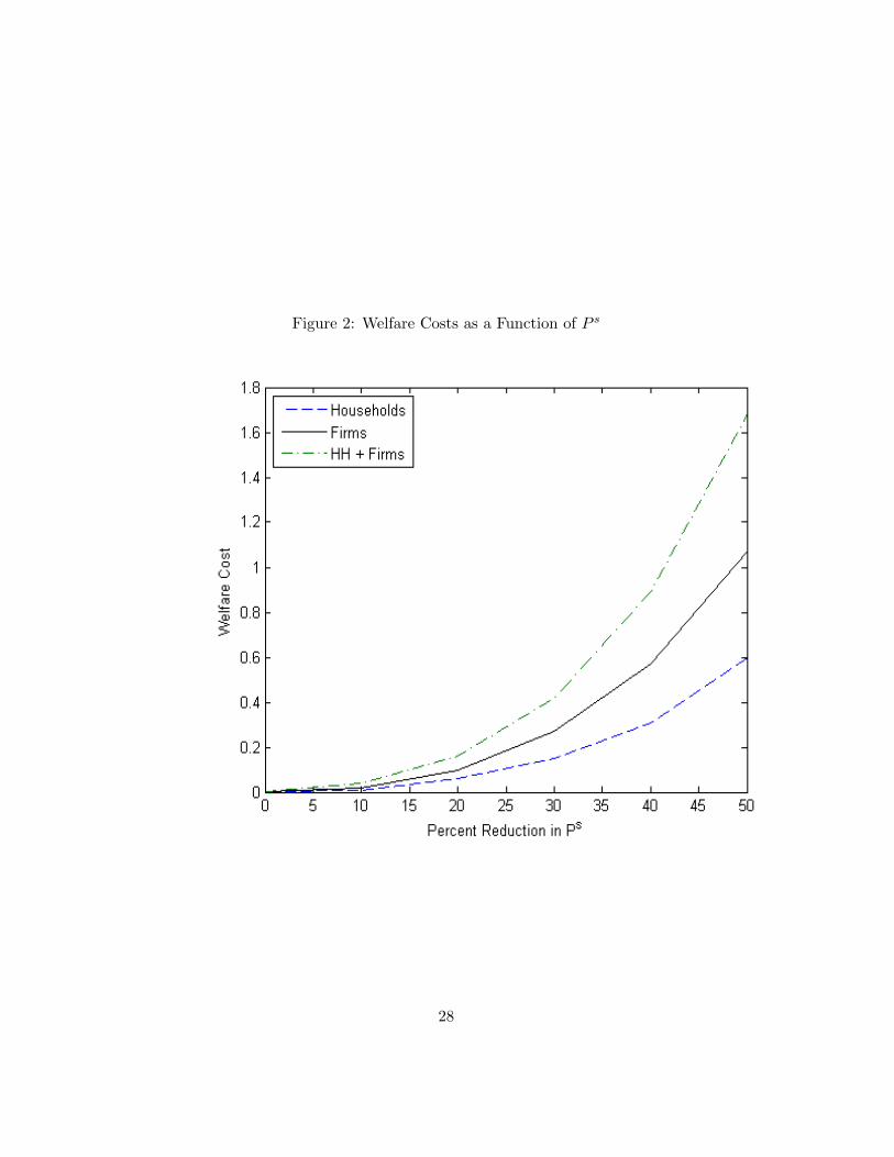
Figure 2: Welfare Costs as a Function of P s

28

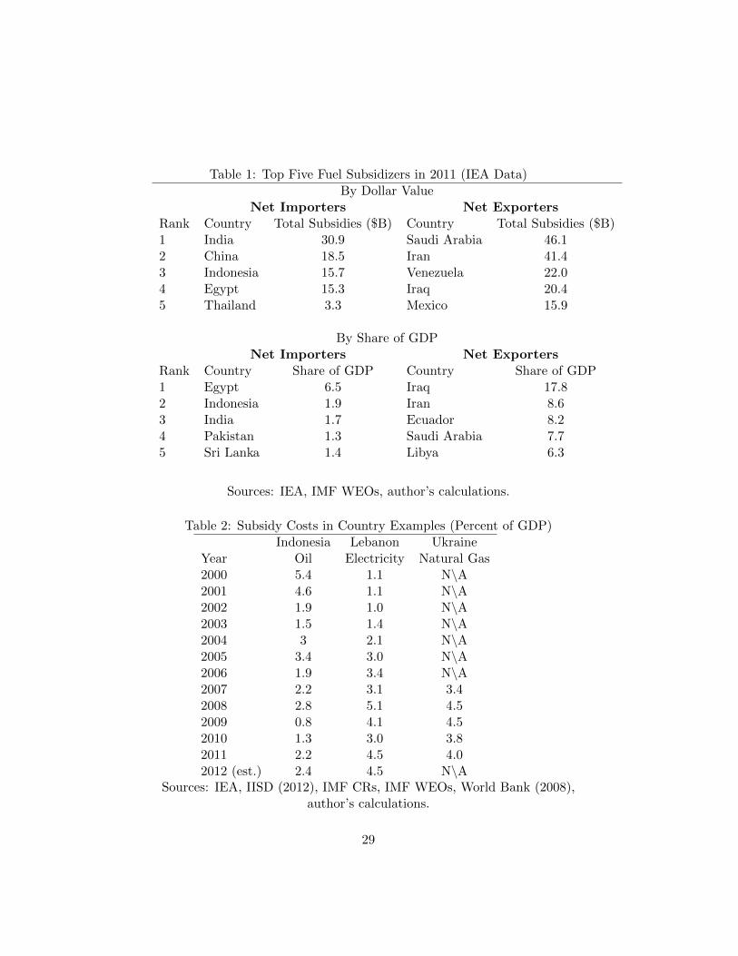
Table 1: Top Five Fuel Subsidizers in 2011 (IEA Data)By Dollar Value

Net Importers Net ExportersRank Country Total Subsidies ($B) Country Total Subsidies ($B)1 India 30.9 Saudi Arabia 46.12 China 18.5 Iran 41.43 Indonesia 15.7 Venezuela 22.04 Egypt 15.3 Iraq 20.45 Thailand 3.3 Mexico 15.9

By Share of GDPNet Importers Net Exporters

Rank Country Share of GDP Country Share of GDP1 Egypt 6.5 Iraq 17.82 Indonesia 1.9 Iran 8.63 India 1.7 Ecuador 8.24 Pakistan 1.3 Saudi Arabia 7.75 Sri Lanka 1.4 Libya 6.3

Sources: IEA, IMF WEOs, author’s calculations.

Table 2: Subsidy Costs in Country Examples (Percent of GDP)Indonesia Lebanon Ukraine

Year Oil Electricity Natural Gas2000 5.4 1.1 N\A2001 4.6 1.1 N\A2002 1.9 1.0 N\A2003 1.5 1.4 N\A2004 3 2.1 N\A2005 3.4 3.0 N\A2006 1.9 3.4 N\A2007 2.2 3.1 3.42008 2.8 5.1 4.52009 0.8 4.1 4.52010 1.3 3.0 3.82011 2.2 4.5 4.02012 (est.) 2.4 4.5 N\A

Sources: IEA, IISD (2012), IMF CRs, IMF WEOs, World Bank (2008),author’s calculations.

29

Tab

le3:

Cal

ibra

tion

Par

amet

eror

vari

able

Valu

eS

ou

rce

Ela

stic

ity

ofin

tert

emp

oral

sub

stit

uti

on

(τ)

.50

Tab

le10.1

inA

gen

or

an

dM

onti

el(1

996)

Ela

stic

itie

sof

sub

stit

uti

on(σc,σT

,σn)

.75,

.25

Gra

ham

an

dG

lais

ter

(2002)

Fri

sch

elas

tici

tyof

lab

orsu

pp

ly(µ

)1,

3S

eed

iscu

ssio

nin

pap

er.

Tim

ep

refe

ren

cera

te(ρ

).0

6R

eal

inte

rest

rate

sin

LD

Cs.

Con

sum

pti

on-e

xp

end

itu

resh

are

ofoil

3%

Est

imate

sfr

om

19

dev

elop

ing

cou

ntr

ies.

Sh

are

ofn

on-t

rad

able

sin

tota

lco

nsu

mp

tion

50%

Bu

ffie

etal.

(2008)

Tot

alfi

rmd

eman

dfo

roi

l5%

of

GD

PIn

pu

t-ou

tpu

tta

ble

sfo

r11

dev

elop

ing

cou

ntr

ies.

Sh

are

ofoi

lu

sed

by

trad

edse

ctor

40%

of

tota

lIn

pu

t-ou

tpu

tta

ble

sfo

r11

dev

elop

ing

cou

ntr

ies.

30

Table 4: Results for Net Oil ImporterAggregate Welfare Costs of Subsidy

Case 1: Households Receive SubsidySubsidy Financed by

Subsidy Cost (% of GDP) Lump-Sum Tax Labor Tax Consumption Tax1 % .11 .11 .122 % .40 .40 .423 % .82 .82 .864 % 1.34 1.34 1.40

Case 2: Firms Receive SubsidySubsidy Financed by

Subsidy Cost (% of GDP) Lump-Sum Tax Labor Tax Consumption Tax1 % .07 .07 .072 % .27 .27 .273 % .57 .56 .564 % .94 .94 .94

Case 3: Household and Firms Receive SubsidySubsidy Financed by


31

Table 5: Results for Net Oil ImporterChanges in Macroeconomic VariablesCase 1: Households Receive Subsidy

Subsidy Financed byVariable Lump-Sum Tax Labor Tax Consumption TaxP s -26.6 -26.6 -26.5Pn 0 0 0CT -0.4 -0.7 -0.8Cn -0.4 -0.7 -0.8Oh 25.5 25.2 25.9WT 0 0 0L 0.4 0.04 0.04LT 1.1 0.7 0.7Ln -0.4 -0.7 -0.8QT 1.1 0.7 0.7Qn -0.4 -0.7 -0.8

Case2: Firms Receive SubsidySubsidy Financed by

Variable Lump-Sum Tax Labor Tax Consumption TaxP s -17.2 -17.3 -17.3Pn -0.5 -0.5 -0.5CT 0.1 -0.2 -0.2Cn 0.5 0.1 0.1Oh 0.1 -0.2 0.5WT 0.7 0.7 0.7L 0.4 0.02 0.02LT 1 0.7 0.7Ln -0.4 -0.7 -0.8QT 1.6 1.2 1.3Qn 0.5 0.1 0.1

Case 3: Households and Firms Receive SubsidySubsidy Financed by

Variable Lump-Sum Tax Labor Tax Consumption TaxP s -11.4 -11.4 -11.4Pn -0.3 -0.3 -0.3CT -0.1 -0.4 -0.4Cn 0.1 -0.2 -0.2Oh 9.4 9.1 9.9WT 0.5 0.5 0.5L 0.3 0.01 0.02LT 1 0.7 0.7Ln -0.4 -0.7 -0.8QT 1.4 1 1Qn 0.1 -0.2 -0.2

32

Table 6: Subsidies vs. Transfers in the Net Oil Importing CaseHouseholds and Firms Receive Subsidy

Labor Tax Consumption TaxCost (% of GDP) Transfers Subsidy Transfers Subsidy

1 .002 .04 .002 .052 .007 .17 .007 .183 .016 .37 .016 .394 .028 .67 .028 .67

Table 7: Aggregate Welfare Costs for the Net Oil ExporterHouseholds and Firms Receive Subsidy

Subsidy Cost (% of GDP) Aggregate Welfare Cost2 % .204 % .706 % 1.428 % 2.28

33

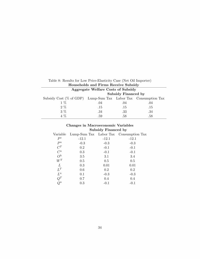
Table 8: Results for Low Price-Elasticity Case (Net Oil Importer)Households and Firms Receive Subsidy

Aggregate Welfare Costs of SubsidySubsidy Financed by


Changes in Macroeconomic VariablesSubsidy Financed by

Variable Lump-Sum Tax Labor Tax Consumption TaxP s -12.1 -12.1 -12.1Pn -0.3 -0.3 -0.3CT 0.2 -0.1 -0.1Cn 0.3 -0.1 -0.1Oh 3.5 3.1 3.4W T 0.5 0.5 0.5L 0.3 0.01 0.01LT 0.6 0.2 0.2Ln 0.1 -0.3 -0.3QT 0.7 0.4 0.4Qn 0.3 -0.1 -0.1

34

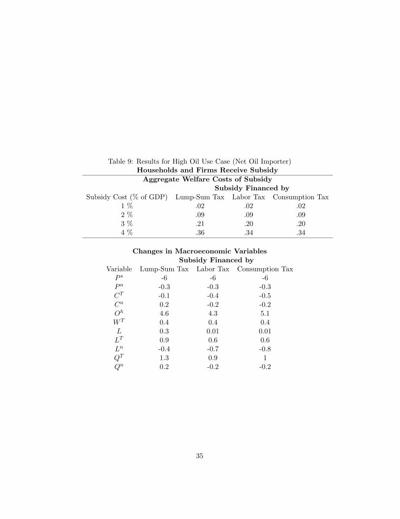
Table 9: Results for High Oil Use Case (Net Oil Importer)Households and Firms Receive Subsidy




Variable Lump-Sum Tax Labor Tax Consumption TaxP s -6 -6 -6Pn -0.3 -0.3 -0.3CT -0.1 -0.4 -0.5Cn 0.2 -0.2 -0.2Oh 4.6 4.3 5.1W T 0.4 0.4 0.4L 0.3 0.01 0.01LT 0.9 0.6 0.6Ln -0.4 -0.7 -0.8QT 1.3 0.9 1Qn 0.2 -0.2 -0.2

35

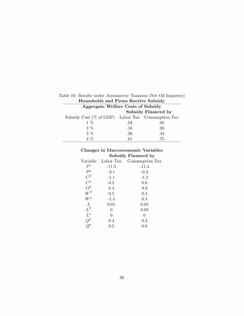
Table 10: Results under Asymmetric Taxation (Net Oil Importer)Households and Firms Receive Subsidy


Subsidy Cost (% of GDP) Labor Tax Consumption Tax1 % .04 .052 % .16 .203 % .36 .444 % .61 .75


Variable Labor Tax Consumption TaxP s -11.5 -11.4Pn -2.1 -0.3CT -1.1 -1.2Cn 0.5 0.6Oh 8.4 9.9W T 0.5 0.4Wn -1.4 0.4L 0.01 0.02LT 0 0.03Ln 0 0QT 0.4 0.4Qn 0.5 0.6

36

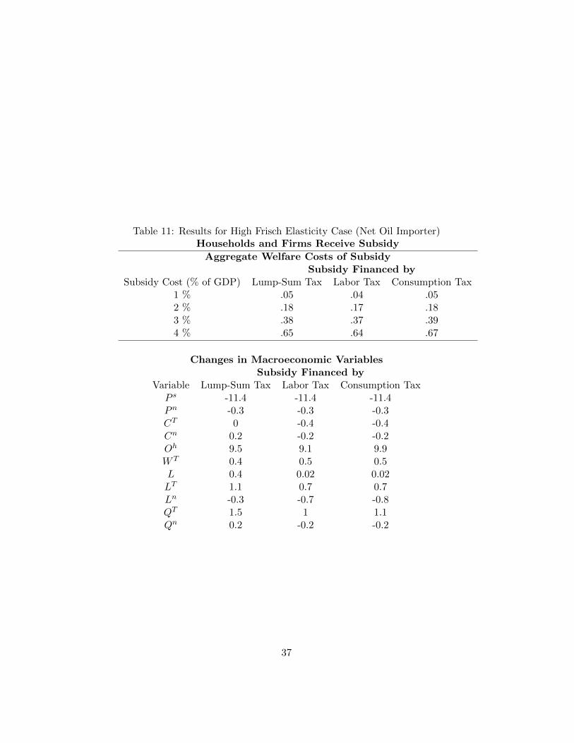
Table 11: Results for High Frisch Elasticity Case (Net Oil Importer)Households and Firms Receive Subsidy




Variable Lump-Sum Tax Labor Tax Consumption TaxP s -11.4 -11.4 -11.4Pn -0.3 -0.3 -0.3CT 0 -0.4 -0.4Cn 0.2 -0.2 -0.2Oh 9.5 9.1 9.9W T 0.4 0.5 0.5L 0.4 0.02 0.02LT 1.1 0.7 0.7Ln -0.3 -0.7 -0.8QT 1.5 1 1.1Qn 0.2 -0.2 -0.2

37

References

Agenor, P., Montiel, P. J., 1996. Development Macroeconomics. PrincetonUniversity Press.

Aissa, M. S. B., Rebei, N., 2012. Price subsidies and the conduct of monetarypolicy. Journal of Macroeconomics 34, 769–787.

Anand, R., Prasad, E. S., 2010. Optimal price indices for targeting inflationunder incomplete markets, NBER Working Paper 16290.

Bacon, R., Bhattacharya, S., Kojima, M., 2010. Expenditure of low-incomehouseholds on energy.Extractive Industries for Development Series No. 16.

Baig, T., Mati, A., Coady, D., Ntamatungiro, J., 2007. Domestic petroleumproduct prices and subsidies: Recent developments and reform strategies,IMF Working Paper, WP/07/71.

Buffie, E., Adam, C., O’Connell, S., Pattillo, C., 2008. Riding the wave:Monetary responses to aid surges in low-income countries. European Eco-nomic Review 52, 1378–1395.

Catao, L., Chang, R., 2010. World food prices and monetary policy, NBERWorking Paper 16563.

Clements, B., Jung, H.-S., Gupta, S., 2003. IMF Working Paper 03/204.

Coady, D., El-Said, M., Gillingham, R., Kpodar, K., Medas, P., Newhouse,D., 2006. The magnitude and distribution of fuel subsidies: Evidencefrom bolivia, ghana, jordan, mali, and sri lanka, IMF Working Paper,WP/06/247.

Coady, D., Gillingham, R., Ossowski, R., Piotrowski, J., Tareq, S., Tyson,J., 2010. Petroleum product subsidies: Costly, inequitable, and rising,IMF Staff Position Note, SPN/10/05.

EIA, 2011. Country analysis brief: Indonesia.

EIA, 2012. International energy statistics.

GIZ, 2010. International fuel prices survey.

Graham, D. J., Glaister, S., 2002. The demand for automobile fuel: A surveyof elasticities. Journal of Transport Economics and Policy 36, 1–26.

38

IEA, 2010. World energy outlook 2010.

IEA, 2011. World energy outlook 2011.

IEA, 2012. Energy policies beyond iea countries: Ukraine 2012.

Ihrig, J., Moe, K., 2004. Lurking in the shadows: the informal sector andgovernment policy. Journal of Development Economics 73, 541–557.

IISD, 2012a. A citzen’s guide to energy subsidies in indonesia: 2012 update,Interntional Institute for Sustainable Development publication.

IISD, 2012b. Indonesia’s fuel subsidies: Action plan for reform, InterntionalInstitute for Sustainable Development publication.

IMF, 2012. Lebanon country report, cr 12/40.

Kpodar, K., 2006. Distributional effects of oil price changes on householdexpenditures: Evidence from mali, IMF Working Paper, WP 06/91.

Larsen, B., Shah, A., 1992. World fossil fuel subsidies and global carbonemissions, World Bank Policy Research Working Paper 1002.

Mitra, P., Atoyan, R., 2012. Ukraine gas policy: Distributional consequencesof tariff increases, IMF Working Paper 12/247.

OECD, 2010. Phasing out energy subsidies, Article in OECD EconomicSurveys: Indonesia 2010.

Petri, M., Taube, G., Tsyvinski, A., 2002. Energy sector quasi-fiscal ac-tivities in the countries of the former soviet union, IMF Working Paper02/60.

Reichling, F., Whalen, C., 2012. Review of estimates of the frisch elasticityof labor supplyCongression Budget Office Working Paper 2012-13.

Vagliasindi, M., 2012. Implementing Energy Subsidy Reforms: Evidencefrom Developing Countries. World Bank.

World Bank, 2007. Program document for a proposed energy developmentpolicy loan to the kingdom of morocco.

World Bank, 2008. Republic of lebanon electricity sector public expenditurereview.

World Bank, 2010. Honduras: Power sector issues and options, ESMAPFormal Report 333/10.

39

A Model equations

(CT

σc−1σc + a1C

nσc−1σc + a2O

hσc−1σc

)( σcσc−1 )(1− 1

τ )−1

CT− 1σc = (1 + τ c)λ (A-1)

(CT

σc−1σc + a1C

nσc−1σc + a2O

hσc−1σc

)( σcσc−1 )(1− 1

τ )−1

a1Cn− 1

σc = (1+τ c)Pnλ (A-2)

(CT

σc−1σc + a1C

nσc−1σc + a2O

hσc−1σc

)( σcσc−1 )(1− 1

τ )−1

a2Oh−

1σc = P sλ (A-3)

κL1µ = (1− τ l)WTλ (A-4)

κL1µ = (1− τ l)Wnλ (A-5)

λ

λ= ρ− r (A-6)

(1− τ l)(WnLn +WTLT

)+ T = (1 + τ c)

(CT − PnCn

)+ P sOh (A-7)

QT =

[(ATLT

)σT−1

σT + bT(OT)σT−1

σT

] σTσT−1

(A-8)

QT1σT(ATLT

)− 1σT AT = WT (A-9)

QT1σT bT

(OT)− 1

σT = P s (A-10)

ΦT =

[(WT

AT

)1−σT+ bT

σT(P s)

1−σT

] 11−σT

(A-11)

Qn =[(AnLn)

σn−1σn + bn (On)

σn−1σn

] σnσn−1

(A-12)

Qn1σn (AnLn)

− 1σn An =

Wn

Pn(A-13)

Qn1σn bn (On)

− 1σn =

P s

Pn(A-14)

Φn =

[(Wn

An

)1−σn+ bnσn (P s)

1−σn

] 11−σn

(A-15)

Cn = Qn (A-16)

b = 0 (A-17)

Government budget constraint for net oil importer

τ l(WTLT +WnLn

)+ τ c

(CT + PnCn

)+ T = Tr + (P o − P s)

(Oh +OT +On

)(A-18)

40

Current account equation for net oil importer

QT = CT + P o(Oh +OT +On

)(A-19)

Government budget constraint for net exporter

P o(Qo −Oh −OT −On

)+ P s

(Oh +OT +On

)= Tr (A-20)

Current account equation for net exporter

QT + P oQo = CT + P o(Oh +OT +On) (A-21)

B Data used for calibration

B.1 Consumption expenditure shares

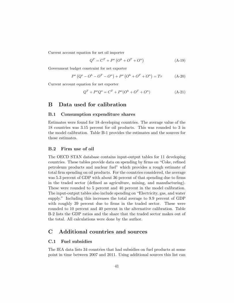
Estimates were found for 18 developing countries. The average value of the18 countries was 3.15 percent for oil products. This was rounded to 3 inthe model calibration. Table B-1 provides the estimates and the sources forthose estimates.

B.2 Firm use of oil

The OECD STAN database contains input-output tables for 11 developingcountries. These tables provide data on spending by firms on “Coke, refinedpetroleum products and nuclear fuel” which provides a rough estimate oftotal firm spending on oil products. For the countries considered, the averagewas 5.3 percent of GDP with about 36 percent of that spending due to firmsin the traded sector (defined as agriculture, mining, and manufacturing).These were rounded to 5 percent and 40 percent in the model calibration.The input-output tables also include spending on “Electricity, gas, and watersupply.” Including this increases the total average to 9.9 percent of GDPwith roughly 39 percent due to firms in the traded sector. These wererounded to 10 percent and 40 percent in the alternative calibration. TableB-2 lists the GDP ratios and the share that the traded sector makes out ofthe total. All calculations were done by the author.

C Additional countries and sources

C.1 Fuel subsidies

The IEA data lists 34 countries that had subsidies on fuel products at somepoint in time between 2007 and 2011. Using additional sources this list can

41

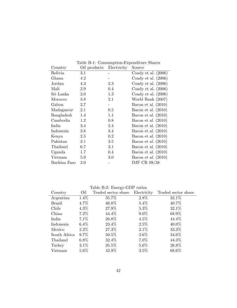
Table B-1: Consumption-Expenditure SharesCountry Oil products Electricity Source

Bolivia 3.1 - Coady et al. (2006)Ghana 4.2 - Coady et al. (2006)Jordan 4.3 2.3 Coady et al. (2006)Mali 2.9 0.4 Coady et al. (2006)Sri Lanka 2.0 1.3 Coady et al. (2006)Morocco 3.8 2.1 World Bank (2007)Gabon 2.7 - Bacon et al. (2010)Madagascar 2.1 0.5 Bacon et al. (2010)Bangladesh 1.4 1.1 Bacon et al. (2010)Cambodia 1.2 0.8 Bacon et al. (2010)India 3.4 2.4 Bacon et al. (2010)Indonesia 3.8 3.4 Bacon et al. (2010)Kenya 2.5 0.2 Bacon et al. (2010)Pakistan 2.1 3.5 Bacon et al. (2010)Thailand 6.7 3.1 Bacon et al. (2010)Uganda 1.7 0.4 Bacon et al. (2010)Vietnam 5.9 3.0 Bacon et al. (2010)Burkina Faso 3.0 - IMF CR 09/38

Table B-2: Energy-GDP ratiosCountry Oil Traded sector share Electricity Traded sector share

Argentina 1.4% 35.7% 2.8% 32.1%Brazil 4.7% 46.8% 5.4% 40.7%Chile 4.3% 27.9% 5.3% 32.1%China 7.2% 44.4% 9.0% 68.9%India 7.1% 26.8% 4.5% 44.4%Indonesia 6.4% 23.4% 2.5% 40.0%Mexico 2.2% 27.3% 2.1% 33.3%South Africa 9.7% 50.5% 2.6% 34.6%Thailand 6.8% 32.4% 7.0% 44.3%Turkey 3.1% 35.5% 5.6% 26.8%Vietnam 5.6% 42.9% 3.5% 68.6%

42

be expanded to include additional countries and to consider years prior to2007. In some cases quantitative data is also available regarding the size of asubsidy in a given year for a country. Table C-1 lists 21 additional countriesidentified as having a fuel subsidy sometime between 2000 and 2012.

C.2 Electricity subsidies

Additional sources also allow one to expand the list of countries with subsi-dies on electricity produced using fossil fuels. Table C-2 lists an additional15 countries that had these subsidies at least one point in time between 2000to 2012.

C.3 Data

Table C-4 provides the fuel subsidy data from the IEA for the 34 coun-tries they identified for the years from 2007 to 2011. The dollar value hasbeen converted into a subsidy-GDP ratio using GDP data from IMF WorldEconomic Outlook reports.

Table C-5 provides additional data on costs of fuel subsidies and elec-tricity subsidies, as a share of GDP. The numbers come from a variety ofsources that have used different methods and data to calculate the costs ofthe subsidies. For this reason comparison across countries or with the IEAdata should be done with extreme caution. Note that there are a number ofgaps in the data. A blank entry does not mean the subsidy was non-existent.It merely means that no data was available for that year.

C.4 Sources

I relied heavily on Vagliasindi (2012), the GIZ International Fuel Pricessurveys, and IMF country reports to identify the additional countries.

Maria Vagliasindi’s book “Implementing Energy Subsidy Reforms: Evi-dence from Developing Countries” provided information on energy subsidiesin 17 countries. Several countries were discussed in the book that are notfound in the IEA data. These included Ghana, Jordan, Morocco, the Do-minican Republic, and Yemen.

The GIZ releases an International Fuel Prices survey every two years.The latest edition is GIZ (2010). These surveys provide a data point forretail gasoline and diesel prices in a number of countries in November everytwo years. The time series for some countries goes back to 1991 but in mostcases does not begin regularly until 1998. The following countries were

43

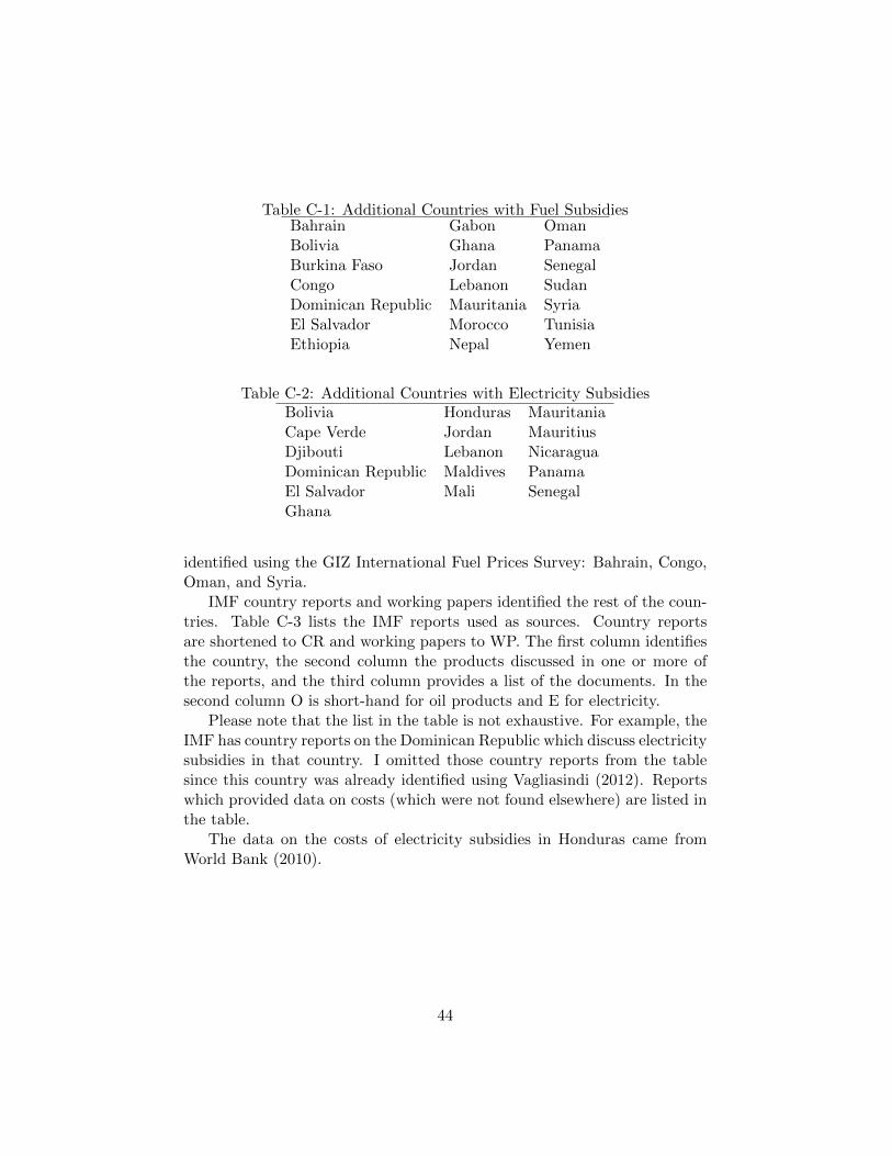
Table C-1: Additional Countries with Fuel SubsidiesBahrain Gabon OmanBolivia Ghana PanamaBurkina Faso Jordan SenegalCongo Lebanon SudanDominican Republic Mauritania SyriaEl Salvador Morocco TunisiaEthiopia Nepal Yemen

Table C-2: Additional Countries with Electricity SubsidiesBolivia Honduras MauritaniaCape Verde Jordan MauritiusDjibouti Lebanon NicaraguaDominican Republic Maldives PanamaEl Salvador Mali SenegalGhana

identified using the GIZ International Fuel Prices Survey: Bahrain, Congo,Oman, and Syria.

IMF country reports and working papers identified the rest of the coun-tries. Table C-3 lists the IMF reports used as sources. Country reportsare shortened to CR and working papers to WP. The first column identifiesthe country, the second column the products discussed in one or more ofthe reports, and the third column provides a list of the documents. In thesecond column O is short-hand for oil products and E for electricity.

Please note that the list in the table is not exhaustive. For example, theIMF has country reports on the Dominican Republic which discuss electricitysubsidies in that country. I omitted those country reports from the tablesince this country was already identified using Vagliasindi (2012). Reportswhich provided data on costs (which were not found elsewhere) are listed inthe table.

The data on the costs of electricity subsidies in Honduras came fromWorld Bank (2010).

44

Table C-3: IMF SourcesCountry Products Reports

Bolivia E, O CR 12/149Burkina Faso O CR 06/359, WP 11/202Cape Verde E CR 10/349, 11/254Djibouti E CR 09/216, 10/277, 12/197El Salvador E, O CR 09/35, 10/307Ethiopia O CR 06/159, 08/259, 08/264, 09/34Gabon O CR 06/238, 08/24, 09/107, 13/55, WP 06/243Honduras E WP 08/168Jordan E, O CR 12/119, 12/120Lebanon E, O CR 04/313, 06/201, 07/382, 09/131, 10/306, 12/39, 12/40Maldives E CR 09/97, 10/28, 10/167, 11/293Mali E CR 11/141, 12/3Mauritania E, O CR 11/362Mauritius E CR 05/281, 08/237Nepal O CR 07/204, 07/366, 08/181, 10/185, 12/326Nicaragua E CR 06/174, 10/376, 11/118, 11/322, 12/256, 12/257Panama E, O CR 06/130, 09/207, 12/83Senegal E, O CR 07/335, 08/221, 09/5, 10/363, 12/337Tunisia O CR 06/207, 08/345, 09/329, 10/282, 12/255

45

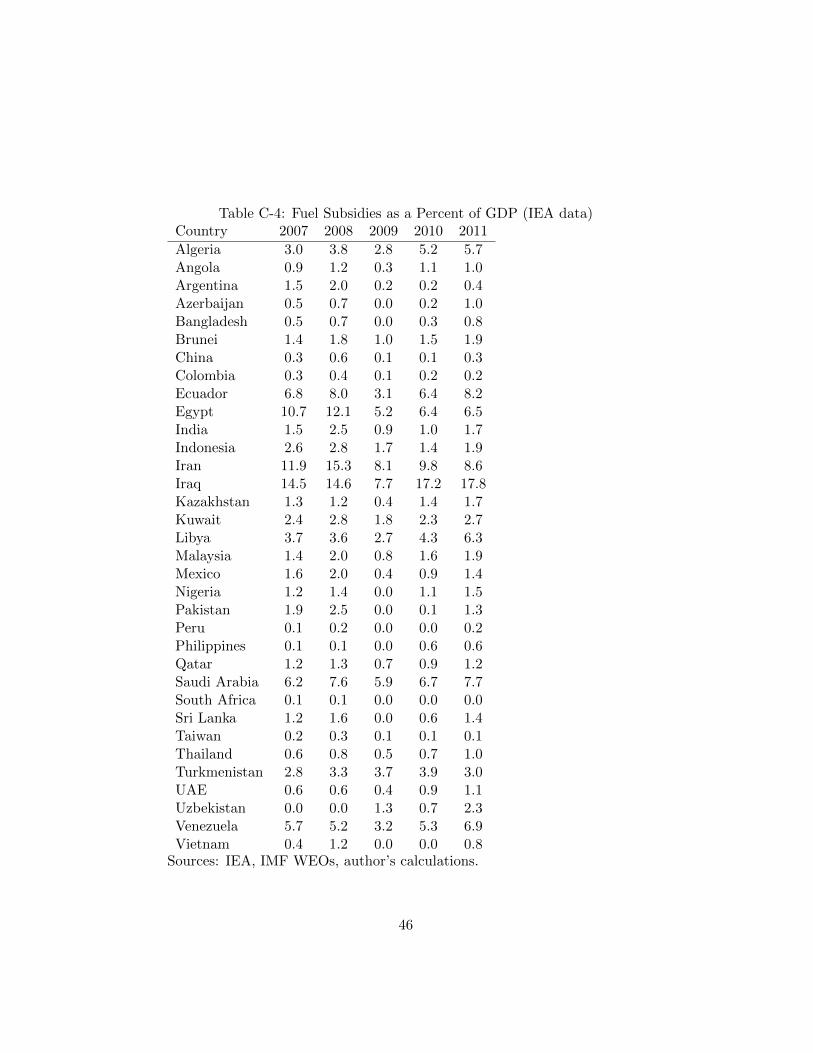
Table C-4: Fuel Subsidies as a Percent of GDP (IEA data)Country 2007 2008 2009 2010 2011

Algeria 3.0 3.8 2.8 5.2 5.7Angola 0.9 1.2 0.3 1.1 1.0Argentina 1.5 2.0 0.2 0.2 0.4Azerbaijan 0.5 0.7 0.0 0.2 1.0Bangladesh 0.5 0.7 0.0 0.3 0.8Brunei 1.4 1.8 1.0 1.5 1.9China 0.3 0.6 0.1 0.1 0.3Colombia 0.3 0.4 0.1 0.2 0.2Ecuador 6.8 8.0 3.1 6.4 8.2Egypt 10.7 12.1 5.2 6.4 6.5India 1.5 2.5 0.9 1.0 1.7Indonesia 2.6 2.8 1.7 1.4 1.9Iran 11.9 15.3 8.1 9.8 8.6Iraq 14.5 14.6 7.7 17.2 17.8Kazakhstan 1.3 1.2 0.4 1.4 1.7Kuwait 2.4 2.8 1.8 2.3 2.7Libya 3.7 3.6 2.7 4.3 6.3Malaysia 1.4 2.0 0.8 1.6 1.9Mexico 1.6 2.0 0.4 0.9 1.4Nigeria 1.2 1.4 0.0 1.1 1.5Pakistan 1.9 2.5 0.0 0.1 1.3Peru 0.1 0.2 0.0 0.0 0.2Philippines 0.1 0.1 0.0 0.6 0.6Qatar 1.2 1.3 0.7 0.9 1.2Saudi Arabia 6.2 7.6 5.9 6.7 7.7South Africa 0.1 0.1 0.0 0.0 0.0Sri Lanka 1.2 1.6 0.0 0.6 1.4Taiwan 0.2 0.3 0.1 0.1 0.1Thailand 0.6 0.8 0.5 0.7 1.0Turkmenistan 2.8 3.3 3.7 3.9 3.0UAE 0.6 0.6 0.4 0.9 1.1Uzbekistan 0.0 0.0 1.3 0.7 2.3Venezuela 5.7 5.2 3.2 5.3 6.9Vietnam 0.4 1.2 0.0 0.0 0.8

Sources: IEA, IMF WEOs, author’s calculations.

46

Tab

leC

-5:

Add

itio

nal

Dat

aon

Su

bsi

dy

Cos

ts2000

2001

2002

2003

2004

2005

2006

2007

2008

2009

2010

2011

2012

FuelSubsidies

Bolivia

0.5

0.9

21.3

1.7

2.9

Burk

ina

Faso

0.7

0.8

Dom

inic

an

Rep

ublic

0.7

0.4

0.5

0.4

0.5

00

0G

ab

on

0.4

0.7

1.6

21

1.3

1.8

Ghana

22.2

1.7

1.5

00.1

0.3

0.3

Indones

ia5.4

4.6

1.9

1.5

33.4

1.9

2.2

2.8

0.8

1.3

2.2

2.4

Jord

an

0.6

1.2

3.2

5.6

2.8

2.7

1.2

0.2

0.4

2.4

1.3

Moro

cco

00.6

1.1

1.4

1.3

3.9

3.7

1.5

1.2

Tunis

ia0.6

1.1

1.2

11.5

0.7

0.9

2.4

2.4

Sen

egal

0.0

0.2

0.3

1.3

1.0

1.2

0.5

0.2

0.2

0.1

Yem

en5.7

3.8

34.8

5.7

8.7

8.1

9.3

14.5

9.5

8.2

Electricity

Subsidies

Dom

inic

an

Rep

ublic

21.7

1.4

1.2

2.7

1.4

1.2

Hondura

s2.6

2.4

2.1

11.3

Indones

ia0.3

0.9

0.8

1.7

0.9

0.9

1.2

1.1

Jord

an

0.9

5.4

Leb

anon

1.1

1.1

1.0

1.4

2.1

3.0

3.4

3.1

5.1

4.1

3.0

4.5

4.5

Mali

0.3

0.4

0.4

Nic

ara

gua

0.6

0.6

Sen

egal

1.8

2.7

1.5

1.6

1.1

1.7

2.1

Yem

en0

00

0.3

0.2

0.2

0.1

0.1

0.1

0.1

0.1

Only

Tota

lAvailable

El

Salv

ador

2.5

1.4

Mauri

tania

0.9

0.8

01.6

2.4

Sourc

es:

Ref

erto

app

endix

.

47

Documents

Michael Plante - Federal Reserve Bank of Dallas ... · Michael Plante Federal Reserve Bank ... Given their cost and persistence, ... them out in the short-run by temporarily limiting