Draft version April 14, 2009Preprint typeset using LATEX style emulateapj v. 6/22/04

MID-INFRARED EXTINCTION MAPPING OF INFRARED DARK CLOUDS:PROBING THE INITIAL CONDITIONS FOR MASSIVE STARS AND STAR CLUSTERS

Michael J. Butler and Jonathan C. TanDepartment of Astronomy, University of Florida, Gainesville, FL 32611, USA;

butler85@astro.ufl.edu, jt@astro.ufl.edu

Draft version April 14, 2009

ABSTRACT

Infrared Dark Clouds (IRDCs) are cold, dense regions of giant molecular clouds that are opaque atwavelengths ∼ 10µm or more and thus appear dark against the diffuse Galactic background emission.They are thought to be the progenitors of massive stars and star clusters. We use 8 µm imagingdata from Spitzer GLIMPSE to make extinction maps of 10 IRDCs, selected to be relatively nearbyand massive. The extinction mapping technique requires construction of a model of the GalacticIR background intensity behind the cloud, which is achieved by correcting for foreground emissionand then interpolating from the surrounding regions. The correction for foreground emission can bequite large, up to ∼ 50% for clouds at ∼ 5 kpc distance, thus restricting the utility of this techniqueto relatively nearby clouds. We investigate three methods for the interpolation, finding systematicdifferences at about the 10% level, which, for fiducial dust models, corresponds to a mass surfacedensity Σ = 0.013g cm−2, above which we conclude this extinction mapping technique attains validity.We examine the probability distribution function of Σ in IRDCs. From a qualitative comparisonwith numerical simulations of astrophysical turbulence, many clouds appear to have relatively narrowdistributions suggesting relatively low (< 5) Mach numbers and/or dynamically strong magnetic fields.Given cloud kinematic distances, we derive cloud masses. Rathborne, Jackson & Simon identified coreswithin the clouds and measured their masses via mm dust emission. For 43 cores, we compare thesemass estimates with those derived from our extinction mapping, finding good agreement: typicallyfactors of . 2 difference for individual cores and an average systematic offset of . 10% for the adoptedfiducial assumptions of each method. We find tentative evidence for a systematic variation of thesemass ratios as a function of core density, which is consistent with models of ice mantle formation ondust grains and subsequent grain growth by coagulation, and/or with a temperature decrease in thedensest cores.Subject headings: ISM: clouds, dust, extinction — stars: formation

1. INTRODUCTION

Large fractions of stars form in clusters from the dens-est clumps within giant molecular clouds (GMCs) (Lada& Lada 2003). These regions are also responsible for thebirth of essentially all massive stars (de Wit et al. 2005).It is possible that our own solar system formed in sucha region near a massive star (Hester et al. 2004), so theprocess of massive star and star cluster formation maybe directly involved in our own origins. Understandingthe formation of star clusters is also important as a foun-dation for understanding global galactic star formationrates (Kennicutt 1998) and thus the evolution of galaxies.

In spite of this importance, there are many gaps inour knowledge of how massive stars and star clusters areformed. For massive star formation there is a basic de-bate about whether the process is simply a scaled-upversion of low-mass star formation from gas cores (Shu,Adams, Lizano 1987), albeit requiring the high pressuresfound in the centers of star-forming clumps (McKee &Tan 2003), or whether a qualitatively different mecha-nism is involved, such as stellar collisions (Bonnell, Bate,Zinnecker 1998) or competitive Bondi-Hoyle accretion(Bonnell et al. 2001; Bonnell, Vine, & Bate 2004). Aprediction of the scenario involving formation from coresis the presence of massive, gravitationally-bound starlesscores as initial conditions.

For star cluster formation there is a debate about

whether the protocluster (or star-forming clump) is inquasi-virial equilibrium (Tan, Krumholz, & McKee 2006)or is undergoing rapid global collapse (Elmegreen 2000,2007; Hartmann & Burkert 2007). This corresponds toa debate about the timescale of star cluster formation:does it take many or just a few free-fall times?

To help resolve these issues we require knowledge aboutthe initial conditions of massive star and star cluster for-mation. The star-forming clumps that are the sites ofthese processes have typically been identified from theradiative emission and activity of their young stars: e.g.radio emission from ultracompact H II regions createdby massive stars or maser emission from hot, dense gasnear massive protostars. Unfortunately by the time thisactivity signposts the region, it has typically also erasedmuch of the memory of the initial conditions from thesystem. This is especially true of protostellar outflows,which have a mechanical power large enough to signifi-cantly stir the gas of the star-forming clump and halt anylarge scale gravitational collapse (Nakamura & Li 2007).

The initial conditions for massive star and star clus-ter formation are expected to be dense, cold cores andclumps of gas. In some formation models there may beof order hundreds of solar masses of gas compressed towithin a few tenths of a parsec. For a spherical cloud the

mean mass surface density, Σ, in this case is

Σ ≡Mc

πR2c

= 0.665Mc

100M⊙

(

Rc

0.1pc

)−2

g cm−2. (1)

For reference, Σ = 1g cm−2 corresponds to 4800M⊙pc−2,NH = 4.3 × 1023 cm−2 and AV ≃ 230 mag, for local dif-fuse ISM dust properties (e.g. Draine 2003). The exten-sion of the extinction law into the mid-infrared (MIR) issomewhat controversial and uncertain (Lutz et al. 1996;Draine 2003; Indebetouw et al. 2005; Roman-Zuniga etal. 2007), but nevertheless, such column densities are ex-pected to correspond to several magnitudes of extinctionat 8 µm.

Such Infrared Dark Clouds (IRDCs) have been iden-tified in images of the Galactic plane from the InfraredSpace Observatory (ISO) (Perault et al. 1996), the Mid-course Space Experiment (MSX) (Egan et al. 1998).Simon et al. (2006a) identified about 10,000 potentialIRDCs from intensity contrast features in the MSX sur-vey. Simon et al. (2006b) identified the 13CO emissionfrom about 300 of the darkest of these in the GalacticRing Survey (GRS) (Jackson et al. 2006), thus derivingtheir kinematic distances. Rathborne, Jackson, & Simon(2006) surveyed the 1.2 mm dust continuum emissionfrom 38 of these IRDCs, identifying 140 mm-emissioncores within these clouds.

The temperatures in IRDCs are measured to be . 20 K(Carey et al. 1998). High deuteration fractions have beenreported by Pillai et al. (2007). Under these conditionsone expects high depletion of volatiles onto ice mantlesof dust grains (Dalgarno & Lepp 1984). Larger molecu-lar line surveys of IRDCs have been carried out by, forexample, Ragan et al. (2006) and Sakai et al. (2008).

In this paper we present a method of extinction map-ping of IRDCs using the diffuse Galactic IR emission ob-served by Spitzer as the background source. This methodcomplements that based on measuring the extinction toindividual stars (e.g. Roman-Zuniga et al. 2007), byproviding a measurement of the extinction at the loca-tion of almost every pixel in the cloud image, includingat very high column densities, thus allowing a detailedinvestigation of the cloud structure.

2. IRDC SAMPLE SELECTION

Considering Spitzer Galactic Legacy Mid-Plane Sur-vey Extraordinaire (GLIMPSE) (Benjamin et al. 2003)8 µm (i.e. Infrared Array Camera [IRAC] band 4) im-ages, we chose 10 IRDCs from the sample of Rathborneet al. (2006), selecting those that were relatively nearby,massive, dark (i.e. showing high contrast compared tothe surrounding diffuse emission), and/or with relativelysimple surrounding diffuse emission. The properties ofthese clouds are listed in Table 1. Apart from beingrelatively nearby, this sub-sample is in fact fairly repre-sentative of the full 38 cloud sample of Rathborne et al.(2006).

Simon et al. (2006a) fit ellipses to each cloud based onMSX images. While these ellipses are often not particu-larly accurate descriptions of the IRDC shapes, we willutilize them as convenient measures of the approximatesizes and shapes of the clouds, especially for the smallscale median filter method of estimating the backgroundradiation (§3.2.2).

The Spitzer telescope has an angular resolution (PSFFWHM) of about 2′′ at 8 µm, which corresponds to alinear scale of 0.029 pc for a cloud at a distance of 3 kpc.Note, GLIMPSE images are processed to a pixel scalecorresponding to an angular resolution of 1.2′′.

3. IRDC EXTINCTION MAPPING METHODS

The extinction mapping technique requires knowingthe intensity of radiation directed towards the observerat a location behind the cloud of interest, Iν,0, and justin front of the cloud, Iν,1. Then for negligible emissionin the cloud and a simplified 1D geometry,

Iν,1 = Iν,0 exp(−τν), (2)

where the optical depth τν = κνΣ, where κν is the totalopacity at frequency ν per unit gas mass and Σ is thegas mass surface density.

To evaluate κν appropriate for the various intensitiesmeasured by the Spitzer Space Telescope, namely the4 IRAC bands and the Multiband Imaging Photometer(MIPS) 24 µm band, we adopt a spectrum of the diffuseGalactic IR emission from Li & Draine (2001), the filterresponse functions of the IRAC and MIPS bands, andperform an intensity and filter response weighted averageof the opacity of various dust models (Figure 1 & Table2). Uncertainties in the dust models include the extentto which ice mantles have formed on the grains and theextent to which the grains have undergone coagulation.

The IR background in the wavelength range probedby the IRAC bands receives its greatest contributionfrom the diffuse ISM (transiently heated small grains)at Band 4, i.e ∼ 8 µm, compared to that from back-ground stars. Individual stellar sources become muchmore prominent in the GLIMPSE images at the shorterwavelengths. Thus in this paper we restrict our analysisto Band 4 images, leaving analysis at other wavelengthsand the wavelength dependence of extinction for a futurestudy.

In the 8 µm band, we estimate a range of dust opac-ities per gas mass of 6.3 − 11 cm2 g−1, and adopt κν =7.5 cm2 g−1, which is formally closest to the model ofOssenkopf & Henning (1994) with thin ice mantles thathave undergone coagulation for 105 yr at a density ofnH = 106 cm−3 (or approximately equivalent to 106 yrat nH = 105 cm−3, etc.).

We estimate Iν,0 via interpolation from the regions sur-rounding the particular IRDC of interest. These inter-polation methods, which necessarily involve an averagingover small scale spatial variations in Iν,0, are describedbelow in §3.2. We evaluate Iν,1 from the observed inten-sities derived from the cloud images. First we considerthe effects of foreground dust emission.

3.1. Correction for Foreground Dust Emission

Our determinations of both Iν,0 and Iν,1 are potentiallyaffected by foreground emission from hot dust. We esti-mate the size of this effect given the (kinematic) distanceto the cloud and a model for the Galactic distribution ofhot dust emission, assuming it is the same as the distri-bution of the Galactic surface density of OB associations(McKee & Williams 1997):

ΣOB ∝ exp

(

−R

HR

)

, (3)

TABLE 1Infrared Dark Cloud Samplea

Cloud Name l b Distance Reff e P.A. ffore ΣSMFb MLMF MSMF

(◦) (◦) ( kpc) (pc) (◦) (g cm−2) (M⊙) (M⊙)

A (G018.82−00.28) 18.822 −0.285 4.8 10.4 0.961 74 0.209 0.0355 6,700 7,600B (G019.27+00.07) 19.271 0.074 2.4 2.71 0.977 88 0.075 0.0387 930 830C (G028.37+00.07) 28.373 0.076 5.0 15.4 0.632 78 0.266 0.0527 27,000 42,000D (G028.53−00.25) 28.531 −0.251 5.7 16.9 0.968 60 0.327 0.0418 17,400 27,000E (G028.67+00.13) 28.677 0.132 5.1 11.5 0.960 103 0.276 0.0543 15,100 19,400F (G034.43+00.24) 34.437 0.245 3.7 3.50 0.926 79 0.193 0.0371 1,770 1,670G (G034.77−00.55) 34.771 −0.557 2.9 3.06 0.953 95 0.140 0.0420 1,050 1,140H (G035.39−00.33) 35.395 −0.336 2.9 9.69 0.951 59 0.142 0.0262 4,000 6,800I (G038.95−00.47) 38.952 −0.475 2.7 3.73 0.917 64 0.141 0.0616 880 1,490J (G053.11+00.05) 53.116 0.054 1.8 0.755 0.583 50 0.121 0.0699 108 80

aCoordinate names, Galactic coordinates, kinematic distances, effective radii (of equal area circles), eccentricitiesand position angles of fitted ellipses are from Simon et al. (2006a).bThis estimate of mean mass surface density, used to normalize the distributions in Fig. 11, is the areal average

of those pixels for which values of ΣSMF > 0 are derived. Estimates of a mean mass surface density based onMSMF and Reff are typically much smaller because of the regions inside the clouds ellipse with ΣSMF ≤ 0.

TABLE 2Spitzer Telescope Band and Background-Weighted Dust Opacities Per Gas Mass (cm2 g−1)

Dust Modela IRAC Band 1 IRAC Band 2 IRAC Band 3 IRAC Band 4 MIPS Band 13.5µmb 4.5µm 5.9µm 7.8µm 23.0µm

WD01 RV = 3.1 10.02 6.26 4.16 6.25 4.50WD01 RV = 3.1 flat IR bkgc 9.78 6.20 4.25 7.71 4.24WD01 RV = 5.5 15.56 10.24 6.55 8.27 5.54WD01 RV = 5.5 case B 14.23 11.49 9.25 10.96 6.01OH94 thin mantle, 0 yr 17.52 (12.69) 10.68 (8.69) 7.78 (7.06) 6.26 (6.15) 4.43OH94 thin mantle, 105yr, 106cm−3 22.41 (16.23) 13.31 (10.83) 9.44 (8.56) 7.48 (7.34) 6.23

aReferences: WD01 - Weingartner & Draine (2001); OH94 - Ossenkopf & Henning (1994), opacities have been scaledfrom values in parentheses to include contribution from scattering.bMean wavelengths weighted by filter response and background spectrum.cNo weighting made for spectrum of Galactic diffuse emission.

where R is the galactocentric radius and HR = 3.5 kpcis the radial scale length. For each IRDC, given its dis-tance and Galactic longitude, we calculate the ratio ofthe column of hot dust between the solar position (atR = 8 kpc) and the total column extending out to agalactocentric radius of 16 kpc. This “Foreground Inten-sity Ratio”, ffore, is listed in Table 1 for each IRDC. Thenwe derive an estimate of the true intensity of the radia-tion field just behind the cloud, Iν,0, from that measuredvia interpolation of the cloud images, Iν,0,obs, via

Iν,0 = (1 − ffore)Iν,0,obs. (4)

We also estimate the true intensity of the radiation fieldjust in front of the cloud, Iν,1 from that measured directlyfrom the cloud images, Iν,1,obs, via

Iν,1 = Iν,1,obs − fforeIν,0,obs. (5)

Typical values of ffore are about 15%, with values upto 33% for the most distant cloud, D, at 5.7 kpc. Asan example of the size of the corrections to Σ result-ing from the foreground subtraction, consider cloud C,for which ffore = 0.266, Iν,0,obs ≃ 100 MJy sr−1 andIν,1,obs ≃ 50 MJy sr−1 in the darkest part of the cloud.For these regions, one would derive Σ ≃ 0.092 g cm−2

without the foreground correction and Σ ≃ 0.152 g cm−2

with this correction.

Our estimate of ffore is uncertain due to small scalespatial variations in the hot dust emission in the Galaxy.Also, we are typically measuring Iν,0,obs from regionsrelatively close to the IRDC of interest. Such regionsare likely to overlap with the GMC hosting the IRDC,and thus have higher than average extinction of the in-tegrated Galactic background emission. This will causeus to tend to underestimate ffore and thus Σ. An upperlimit to ffore is provided by the minimum value of Iν,1,obs

for each cloud. For example, for Cloud C this is about40 MJy sr−1 intensity units, so that for a background of100 MJy sr−1, the maximum value of ffore ≃ 0.4. Uncer-tainties in ffore are one of the major reasons for restrict-ing the extinction mapping analysis to relatively nearbyclouds.

3.2. Background Estimation

3.2.1. Large-Scale Median Filter (LMF)

A relatively simple way of estimating the diffuse IRbackground at a given location behind an IRDC is totake a median average of a region (i.e. filter) centeredon the location of interest and that is large comparedto the cloud. This method was applied by Simon et al.(2006a) to model the Galactic background from MSXimages to then identify IRDCs as high contrast features.

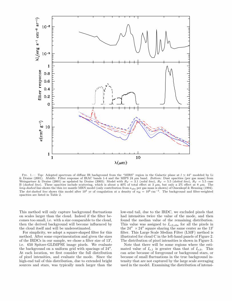
Fig. 1.— Top: Adopted spectrum of diffuse IR background from the “MIRS” region in the Galactic plane at l ≃ 44◦ modeled by Li& Draine (2001). Middle: Filter response of IRAC bands 1-4 and the MIPS 24 µm band. Bottom: Dust opacities (per gas mass) fromWeingartner & Draine (2001) as updated by Draine (2003): Model with RV = 3.1 (solid line), RV = 5.5 (dotted line), RV = 5.5 caseB (dashed line). These opacities include scattering, which is about a 40% of total effect at 3 µm, but only a 2% effect at 8 µm. Thelong-dashed line shows the thin ice mantle MRN model (only contribution from κabs per gas mass is shown) of Ossenkopf & Henning (1994).The dot-dashed line shows this model after 105 yr of coagulation at a density of nH = 106 cm−3. The background and filter-weightedopacities are listed in Table 2.

This method will only capture background fluctuationson scales larger than the cloud. Indeed if the filter be-comes too small, i.e. with a size comparable to the cloud,then the derived background will become influenced bythe cloud itself and will be underestimated.

For simplicity, we adopt a square-shaped filter for thismethod. After some experimentation and given the sizesof the IRDCs in our sample, we chose a filter size of 13′,i.e. 650 Spitzer-GLIMPSE image pixels. We evaluatethe background on a uniform grid with spacings of 24′′.At each location, we first consider the full distributionof pixel intensities, and evaluate the mode. Since thehigh-end tail of this distribution, due to extended brightsources and stars, was typically much larger than the

low-end tail, due to the IRDC, we excluded pixels thathad intensities twice the value of the mode, and thenfound the median value of the remaining distribution.This value was assigned to Iν,0,obs for all the pixels inthe 24′′ × 24′′ square sharing the same center as the 13′

filter. This Large Scale Median Filter (LMF) method isillustrated for cloud C in the left-hand panels of Figure 2.The distribution of pixel intensities is shown in Figure 3.

Note that there will be some regions where the esti-mated value of Iν,1 is greater than that of Iν,0. Thiscan arise because of foreground or background stars, orbecause of small fluctuations in the true background in-tensity that are not captured by the large scale averagingused in the model. Examining the distribution of intensi-

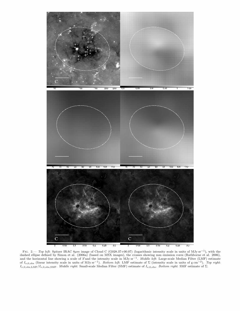
Fig. 2.— Top left: Spitzer IRAC 8µm image of Cloud C (G028.37+00.07) (logarithmic intensity scale in units of MJy sr−1), with thedashed ellipse defined by Simon et al. (2006a) (based on MSX images), the crosses showing mm emission cores (Rathborne et al. 2006),and the horizontal line showing a scale of 3′and the intensity scale in MJy sr−1. Middle left: Large-scale Median Filter (LMF) estimateof Iν,0,obs (linear intensity scale in units of MJy sr−1). Bottom left: LMF estimate of Σ (intensity scale in units of g cm−2). Top right:Iν,0,obs,LMF/Iν,0,obs,SMF. Middle right: Small-scale Median Filter (SMF) estimate of Iν,0,obs. Bottom right: SMF estimate of Σ.

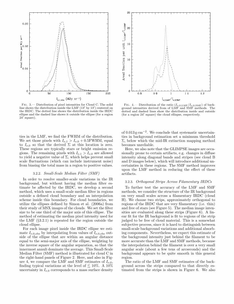
Fig. 3.— Distribution of pixel intensities for Cloud C. The solidline shows the distribution inside the LMF (13′ by 13′) centered onthe IRDC. The dotted line shows the distribution inside the IRDCellipse and the dashed line shows it outside the ellipse (for a region24′ square).

ties in the LMF, we find the FWHM of the distribution.We set those pixels with Iν,1 > Iν,0 + 0.5FWHM, equalto Iν,0 so that the derived Σ at this location is zero.These regions are typically stars or bright emission re-gions. The remaining pixels with Iν,1 > Iν,0 are allowedto yield a negative value of Σ, which helps prevent smallscale fluctuations (which can include instrument noise)from biasing the total mass in a region to positive values.

3.2.2. Small-Scale Median Filter (SMF)

In order to resolve smaller-scale variations in the IRbackground, but without having the median filter es-timate be affected by the IRDC, we develop a secondmethod, which uses a small-scale median filter in regionsoutside a defined cloud boundary and an interpolationscheme inside this boundary. For cloud boundaries, weutilize the ellipses defined by Simon et al. (2006a) fromtheir study of MSX images of the clouds. We set the filtersize to be one third of the major axis of this ellipse. Themethod of estimating the median pixel intensity used forthe LMF (§3.2.1) is repeated for the region outside thecloud ellipse.

For each image pixel inside the IRDC ellipse we esti-mate Iν,0,obs by interpolating from values of Iν,0,obs out-side of the ellipse that are within an angular distanceequal to the semi-major axis of the ellipse, weighting bythe inverse square of the angular separation, so that theinnermost annuli dominate the average. This Small-ScaleMedian Filter (SMF) method is illustrated for cloud C inthe right-hand panels of Figure 2. Here, and also in Fig-ure 4, we compare the LMF and SMF estimates of Iν,0,finding typical variations at the level of . 10%. A 10%uncertainty in Iν,0 corresponds to a mass surface density

Fig. 4.— Distribution of the ratio (Iν,0,LMF/Iν,0,SMF) of back-ground intensities derived from of LMF and SMF methods. Thedotted and dashed lines show the distribution inside and outside(for a region 24′ square) the cloud ellispse, respectively.

of 0.013 g cm−2. We conclude that systematic uncertain-ties in background estimation set a minimum thresholdΣ, below which the mid-IR extinction mapping methodbecomes unreliable.

Here, we also note that the GLIMPSE images are occa-sionally prone to certain artifacts, e.g. changes in diffuseintensity along diagonal bands and stripes (see cloud Band D images below), which will introduce additional un-certainties in these regions. The SMF method improvesupon the LMF method in reducing the effect of theseartifacts.

3.2.3. Orthogonal Strips Across Filamentary IRDCs

To further test the accuracy of the LMF and SMFmethods, we consider the structure of the IR backgroundon very small scales across a filamentary IRDC (cloudH). We choose two strips, approximately orthogonal toregions of the IRDC that are very filamentary (i.e. thin)and free of stars (see Figure 5). The median image inten-sities are evaluated along these strips (Figure 6). A lin-ear fit for the IR background is fit to regions of the stripjudged to be free of cloud material. This is a somewhatsubjective process, since it is hard to distinguish betweensmall-scale background variations and additional absorb-ing components. Nevertheless, we expect this estimate ofthe background intensity just behind the filament to bemore accurate than the LMF and SMF methods, becausethe interpolation behind the filament is over a very smallangular scale (about a few tens of arcseconds) and thebackground appears to be quite smooth in this generalregion.

The ratio of the LMF and SMF estimates of the back-ground across the strips compared to that directly es-timated from the strips is shown in Figure 6. We also

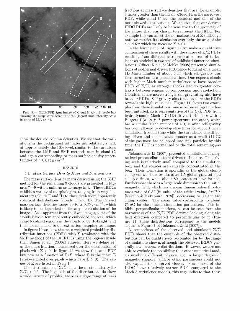
Fig. 5.— GLIMPSE 8µm image of Cloud H with 3′ scale barshowing the strips considered in §3.2.3 (logarithmic intensity scalein units of MJy sr−1).

show the derived column densities. We see that the vari-ations in the background estimates are relatively small,at approximately the 10% level, similar to the variationsbetween the LMF and SMF methods seen in cloud C,and again corresponding to mass surface density uncer-tainties of ≃ 0.013 g cm−2.

4. RESULTS

4.1. Mass Surface Density Maps and Distributions

The mass surface density maps derived using the SMFmethod for the remaining 9 clouds are presented in Fig-ures 7—9 with a uniform scale range in Σ. These IRDCsexhibit a variety of morphologies, ranging from very fila-mentary (clouds F and H) to those with more apparentlyspherical distributions (clouds C and E). The derivedmass surface densities range up to ≃ 0.35 g cm−2, whichis likely to be dependent on the angular resolution of theimages. As is apparent from the 8 µm images, some of theclouds have a few apparently embedded sources, whichcause localized regions in the clouds to be IR-bright, andthus not amenable to our extinction mapping technique.

In figure 10 we show the mass-weighted probability dis-tribution functions (PDFs) with Σ (evaluated with theSMF method) of the 10 IRDCs using the regions insidetheir Simon et al. (2006a) ellipses. Here we define M ′

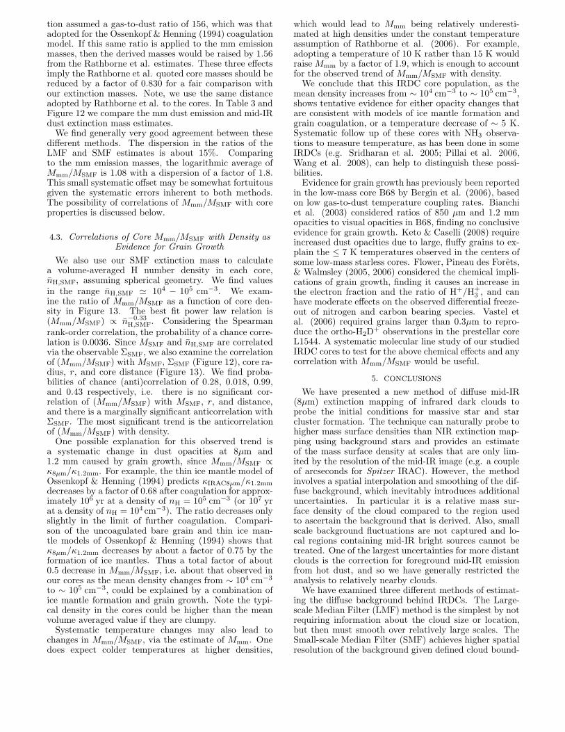
as the mass fraction, normalized over the distribution ofpixels with Σ > 0. In figure 11 we show the same PDFbut now as a function of Σ/Σ, where Σ is the mean Σ(area-weighted over pixels which have Σ > 0). The val-ues of Σ are listed in Table 1.

The distributions of Σ/Σ show the most similarity forΣ/Σ < 0.5. The high-side of the distributions do showa wide variety of profiles: there is a large range of mass

fractions at mass surface densities that are, for example,3 times greater than the mean. Cloud J has the narrowestPDF, while cloud C has the broadest and one of themost skewed distributions. We caution that our derivedIRDC PDFs are likely to be sensitive to the geometry ofthe ellipse that was chosen to represent the IRDC. Forexample this can affect the normalization of Σ (althoughnote we restrict its calculation over only the area of thecloud for which we measure Σ > 0).

In the lower panel of Figure 11 we make a qualitativecomparison of these results with the shapes of Σ/Σ PDFsresulting from different astrophysical sources of turbu-lence as modeled in two sets of published numerical simu-lations. Offner, Klein, & McKee (2008) presented simula-tions of isothermal driven turbulence to maintain a mean1D Mach number of about 5 in which self-gravity wasthen turned on at a particular time. One expects cloudswith higher Mach number turbulence to have broaderPDFs of Σ/Σ, as stronger shocks lead to greater con-trasts between regions of compression and rarefaction.Clouds that are more strongly self-gravitating also havebroader PDFs. Self-gravity also tends to skew the PDFstowards the high-value side. Figure 11 shows two exam-ples from these simulations: one is before self-gravity hasbeen initiated, so is representative of the Σ/Σ PDF fromhydrodynamic Mach 4.7 (1D) driven turbulence with aBurgers P (k) ∝ k−2 power spectrum; the other, whichhas a similar Mach number of 4.9, is after self-gravityhas been allowed to develop structures for about 1 meansimulation free-fall time while the turbulence is still be-ing driven and is somewhat broader as a result (14.2%of the gas mass has collapsed into sink particles by thistime; the PDF is normalized to the total remaining gasmass).

Nakamura & Li (2007) presented simulations of mag-netized protostellar outflow driven turbulence. The driv-ing scale is relatively small compared to the simulationbox, and the sources are centrally concentrated in thebox. Their formation is sporadic as the global clumpcollapses: we show results after 1.5 global gravitationalcollapse times, when about 80 protostars have formed.Furthermore there is a large scale direction to the initialmagnetic field, which has a mean dimensionless flux-to-mass ratio of 0.52 (in units of the critical value, 2πG1/2

[Nakano & Nakamura 1978]), decreasing to 0.19 in theclump center. The mean value corresponds to about75 µG for the fiducial simulation parameters. This in-hibits perpendicular motions, as can be seen from thenarrowness of the Σ/Σ PDF derived looking along thefield direction compared to perpendicular to it (Fig-ure 11; these distributions correspond to the modelsshown in Figure 7 of Nakamura & Li [2007]).

A comparison of the observed and simulated Σ/ΣPDFs shows that the ensemble of the observed distri-butions can be qualitatively accounted for by the rangeof simulations shown, although the observed IRDCs gen-erally have narrower distributions. However, we are notable to exclude the possibility that other numerical mod-els involving different physics, e.g. a larger degree ofmagnetic support, and/or other parameters could notalso explain the observed clouds. Since most of theIRDCs have relatively narrow PDFs compared to theMach 5 turbulence models, this may indicate that these

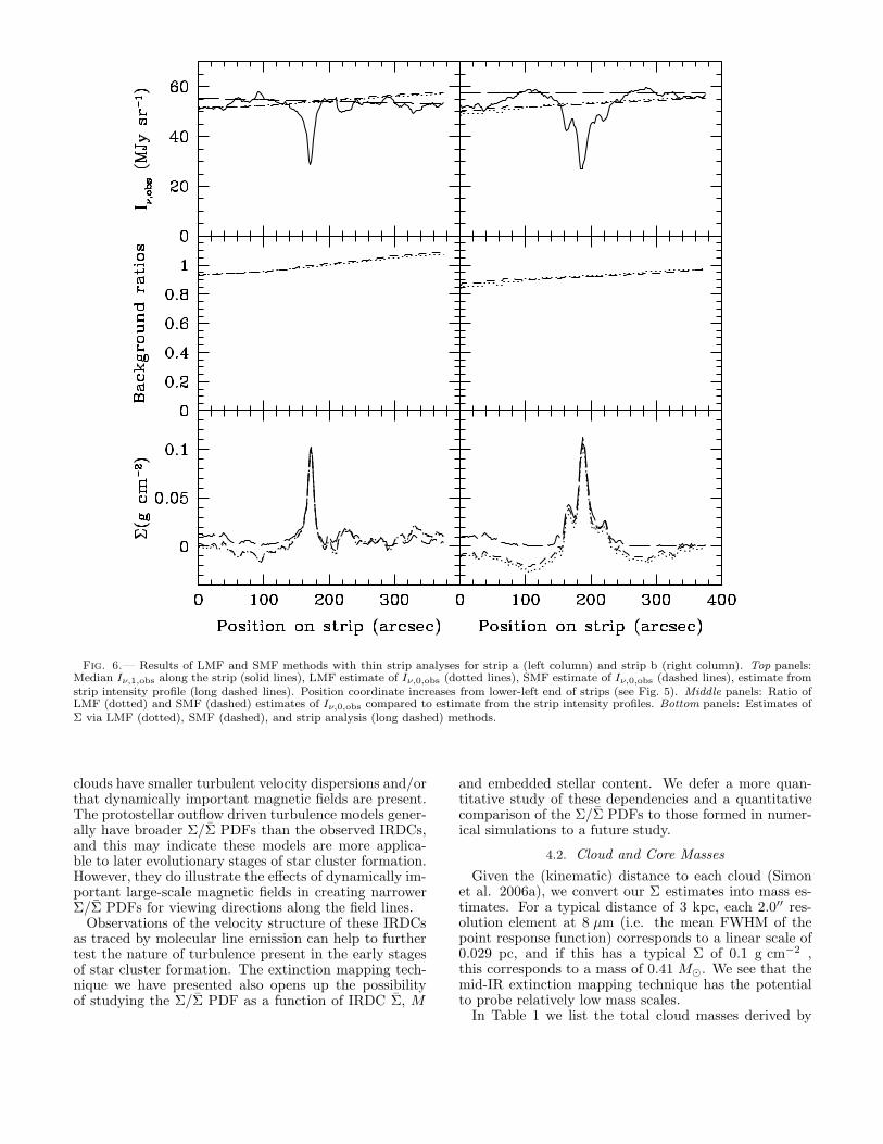
Fig. 6.— Results of LMF and SMF methods with thin strip analyses for strip a (left column) and strip b (right column). Top panels:Median Iν,1,obs along the strip (solid lines), LMF estimate of Iν,0,obs (dotted lines), SMF estimate of Iν,0,obs (dashed lines), estimate fromstrip intensity profile (long dashed lines). Position coordinate increases from lower-left end of strips (see Fig. 5). Middle panels: Ratio ofLMF (dotted) and SMF (dashed) estimates of Iν,0,obs compared to estimate from the strip intensity profiles. Bottom panels: Estimates ofΣ via LMF (dotted), SMF (dashed), and strip analysis (long dashed) methods.

clouds have smaller turbulent velocity dispersions and/orthat dynamically important magnetic fields are present.The protostellar outflow driven turbulence models gener-ally have broader Σ/Σ PDFs than the observed IRDCs,and this may indicate these models are more applica-ble to later evolutionary stages of star cluster formation.However, they do illustrate the effects of dynamically im-portant large-scale magnetic fields in creating narrowerΣ/Σ PDFs for viewing directions along the field lines.

Observations of the velocity structure of these IRDCsas traced by molecular line emission can help to furthertest the nature of turbulence present in the early stagesof star cluster formation. The extinction mapping tech-nique we have presented also opens up the possibilityof studying the Σ/Σ PDF as a function of IRDC Σ, M

and embedded stellar content. We defer a more quan-titative study of these dependencies and a quantitativecomparison of the Σ/Σ PDFs to those formed in numer-ical simulations to a future study.

4.2. Cloud and Core Masses

Given the (kinematic) distance to each cloud (Simonet al. 2006a), we convert our Σ estimates into mass es-timates. For a typical distance of 3 kpc, each 2.0′′ res-olution element at 8 µm (i.e. the mean FWHM of thepoint response function) corresponds to a linear scale of0.029 pc, and if this has a typical Σ of 0.1 g cm−2 ,this corresponds to a mass of 0.41 M⊙. We see that themid-IR extinction mapping technique has the potentialto probe relatively low mass scales.

In Table 1 we list the total cloud masses derived by

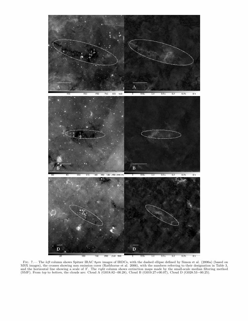
Fig. 7.— The left column shows Spitzer IRAC 8µm images of IRDCs, with the dashed ellipse defined by Simon et al. (2006a) (based onMSX images), the crosses showing mm emission cores (Rathborne et al. 2006), with the numbers referring to their designation in Table 3,and the horizontal line showing a scale of 3′. The right column shows extinction maps made by the small-scale median filtering method(SMF). From top to bottom, the clouds are: Cloud A (G018.82−00.28), Cloud B (G019.27+00.07), Cloud D (G028.53−00.25).

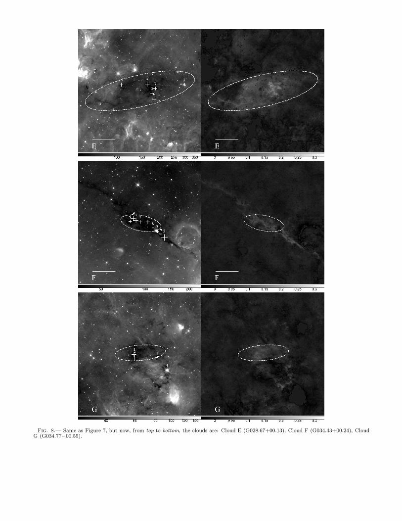
Fig. 8.— Same as Figure 7, but now, from top to bottom, the clouds are: Cloud E (G028.67+00.13), Cloud F (G034.43+00.24), CloudG (G034.77−00.55).

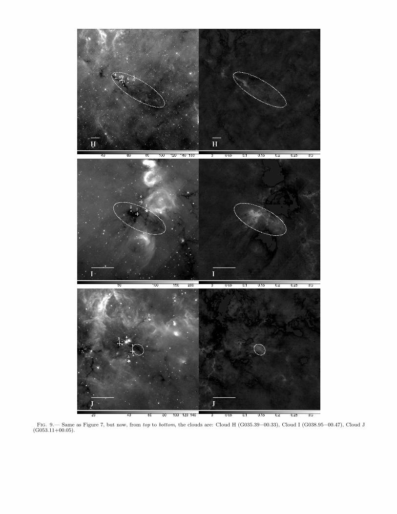
Fig. 9.— Same as Figure 7, but now, from top to bottom, the clouds are: Cloud H (G035.39−00.33), Cloud I (G038.95−00.47), Cloud J(G053.11+00.05).

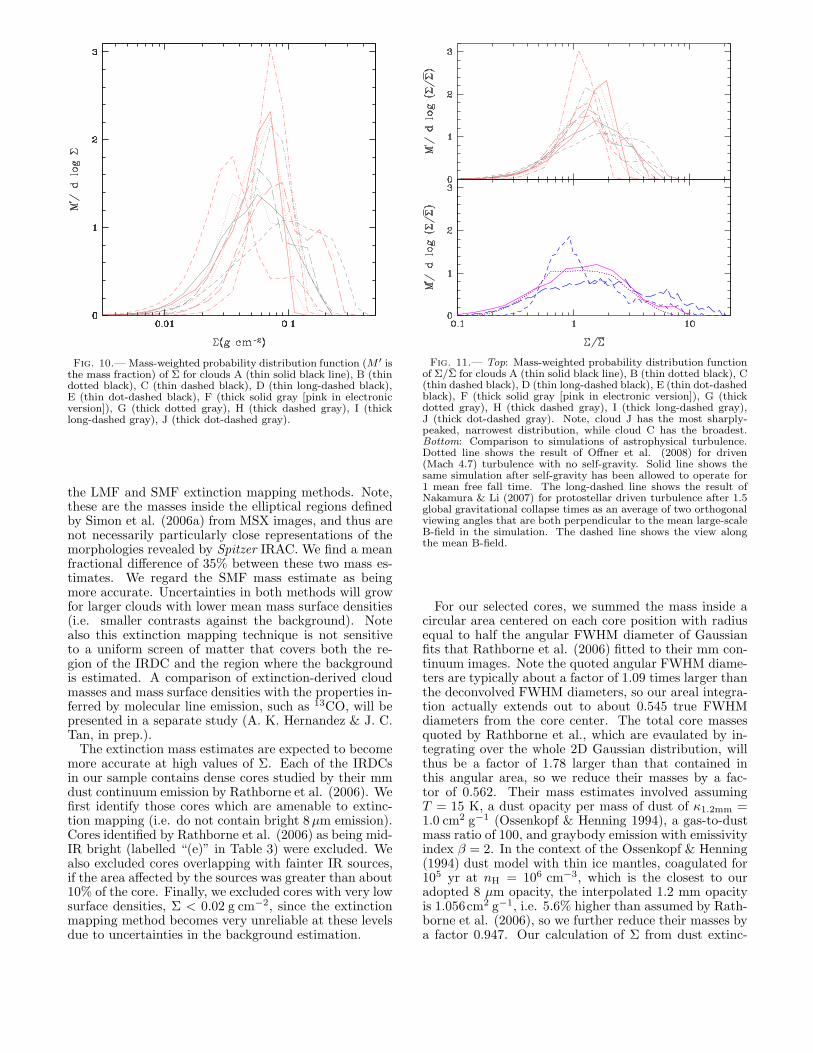
Fig. 10.— Mass-weighted probability distribution function (M ′ isthe mass fraction) of Σ for clouds A (thin solid black line), B (thindotted black), C (thin dashed black), D (thin long-dashed black),E (thin dot-dashed black), F (thick solid gray [pink in electronicversion]), G (thick dotted gray), H (thick dashed gray), I (thicklong-dashed gray), J (thick dot-dashed gray).

the LMF and SMF extinction mapping methods. Note,these are the masses inside the elliptical regions definedby Simon et al. (2006a) from MSX images, and thus arenot necessarily particularly close representations of themorphologies revealed by Spitzer IRAC. We find a meanfractional difference of 35% between these two mass es-timates. We regard the SMF mass estimate as beingmore accurate. Uncertainties in both methods will growfor larger clouds with lower mean mass surface densities(i.e. smaller contrasts against the background). Notealso this extinction mapping technique is not sensitiveto a uniform screen of matter that covers both the re-gion of the IRDC and the region where the backgroundis estimated. A comparison of extinction-derived cloudmasses and mass surface densities with the properties in-ferred by molecular line emission, such as 13CO, will bepresented in a separate study (A. K. Hernandez & J. C.Tan, in prep.).

The extinction mass estimates are expected to becomemore accurate at high values of Σ. Each of the IRDCsin our sample contains dense cores studied by their mmdust continuum emission by Rathborne et al. (2006). Wefirst identify those cores which are amenable to extinc-tion mapping (i.e. do not contain bright 8 µm emission).Cores identified by Rathborne et al. (2006) as being mid-IR bright (labelled “(e)” in Table 3) were excluded. Wealso excluded cores overlapping with fainter IR sources,if the area affected by the sources was greater than about10% of the core. Finally, we excluded cores with very lowsurface densities, Σ < 0.02 g cm−2, since the extinctionmapping method becomes very unreliable at these levelsdue to uncertainties in the background estimation.

Fig. 11.— Top: Mass-weighted probability distribution functionof Σ/Σ for clouds A (thin solid black line), B (thin dotted black), C(thin dashed black), D (thin long-dashed black), E (thin dot-dashedblack), F (thick solid gray [pink in electronic version]), G (thickdotted gray), H (thick dashed gray), I (thick long-dashed gray),J (thick dot-dashed gray). Note, cloud J has the most sharply-peaked, narrowest distribution, while cloud C has the broadest.Bottom: Comparison to simulations of astrophysical turbulence.Dotted line shows the result of Offner et al. (2008) for driven(Mach 4.7) turbulence with no self-gravity. Solid line shows thesame simulation after self-gravity has been allowed to operate for1 mean free fall time. The long-dashed line shows the result ofNakamura & Li (2007) for protostellar driven turbulence after 1.5global gravitational collapse times as an average of two orthogonalviewing angles that are both perpendicular to the mean large-scaleB-field in the simulation. The dashed line shows the view alongthe mean B-field.

For our selected cores, we summed the mass inside acircular area centered on each core position with radiusequal to half the angular FWHM diameter of Gaussianfits that Rathborne et al. (2006) fitted to their mm con-tinuum images. Note the quoted angular FWHM diame-ters are typically about a factor of 1.09 times larger thanthe deconvolved FWHM diameters, so our areal integra-tion actually extends out to about 0.545 true FWHMdiameters from the core center. The total core massesquoted by Rathborne et al., which are evaulated by in-tegrating over the whole 2D Gaussian distribution, willthus be a factor of 1.78 larger than that contained inthis angular area, so we reduce their masses by a fac-tor of 0.562. Their mass estimates involved assumingT = 15 K, a dust opacity per mass of dust of κ1.2mm =1.0 cm2 g−1 (Ossenkopf & Henning 1994), a gas-to-dustmass ratio of 100, and graybody emission with emissivityindex β = 2. In the context of the Ossenkopf & Henning(1994) dust model with thin ice mantles, coagulated for105 yr at nH = 106 cm−3, which is the closest to ouradopted 8 µm opacity, the interpolated 1.2 mm opacityis 1.056cm2 g−1, i.e. 5.6% higher than assumed by Rath-borne et al. (2006), so we further reduce their masses bya factor 0.947. Our calculation of Σ from dust extinc-

tion assumed a gas-to-dust ratio of 156, which was thatadopted for the Ossenkopf & Henning (1994) coagulationmodel. If this same ratio is applied to the mm emissionmasses, then the derived masses would be raised by 1.56from the Rathborne et al. estimates. These three effectsimply the Rathborne et al. quoted core masses should bereduced by a factor of 0.830 for a fair comparison withour extinction masses. Note, we use the same distanceadopted by Rathborne et al. to the cores. In Table 3 andFigure 12 we compare the mm dust emission and mid-IRdust extinction mass estimates.

We find generally very good agreement between thesedifferent methods. The dispersion in the ratios of theLMF and SMF estimates is about 15%. Comparingto the mm emission masses, the logarithmic average ofMmm/MSMF is 1.08 with a dispersion of a factor of 1.8.This small systematic offset may be somewhat fortuitousgiven the systematic errors inherent to both methods.The possibility of correlations of Mmm/MSMF with coreproperties is discussed below.

4.3. Correlations of Core Mmm/MSMF with Density asEvidence for Grain Growth

We also use our SMF extinction mass to calculatea volume-averaged H number density in each core,nH,SMF, assuming spherical geometry. We find valuesin the range nH,SMF ≃ 104 − 105 cm−3. We exam-ine the ratio of Mmm/MSMF as a function of core den-sity in Figure 13. The best fit power law relation is(Mmm/MSMF) ∝ n−0.33

H,SMF. Considering the Spearmanrank-order correlation, the probability of a chance corre-lation is 0.0036. Since MSMF and nH,SMF are correlatedvia the observable ΣSMF, we also examine the correlationof (Mmm/MSMF) with MSMF, ΣSMF (Figure 12), core ra-dius, r, and core distance (Figure 13). We find proba-bilities of chance (anti)correlation of 0.28, 0.018, 0.99,and 0.43 respectively, i.e. there is no significant cor-relation of (Mmm/MSMF) with MSMF, r, and distance,and there is a marginally significant anticorrelation withΣSMF. The most significant trend is the anticorrelationof (Mmm/MSMF) with density.

One possible explanation for this observed trend isa systematic change in dust opacities at 8µm and1.2 mm caused by grain growth, since Mmm/MSMF ∝κ8µm/κ1.2mm. For example, the thin ice mantle model ofOssenkopf & Henning (1994) predicts κIRAC8µm/κ1.2mm

decreases by a factor of 0.68 after coagulation for approx-imately 106 yr at a density of nH = 105 cm−3 (or 107 yrat a density of nH = 104 cm−3). The ratio decreases onlyslightly in the limit of further coagulation. Compari-son of the uncoagulated bare grain and thin ice man-tle models of Ossenkopf & Henning (1994) shows thatκ8µm/κ1.2mm decreases by about a factor of 0.75 by theformation of ice mantles. Thus a total factor of about0.5 decrease in Mmm/MSMF, i.e. about that observed inour cores as the mean density changes from ∼ 104 cm−3

to ∼ 105 cm−3, could be explained by a combination ofice mantle formation and grain growth. Note the typi-cal density in the cores could be higher than the meanvolume averaged value if they are clumpy.

Systematic temperature changes may also lead tochanges in Mmm/MSMF, via the estimate of Mmm. Onedoes expect colder temperatures at higher densities,

which would lead to Mmm being relatively underesti-mated at high densities under the constant temperatureassumption of Rathborne et al. (2006). For example,adopting a temperature of 10 K rather than 15 K wouldraise Mmm by a factor of 1.9, which is enough to accountfor the observed trend of Mmm/MSMF with density.

We conclude that this IRDC core population, as themean density increases from ∼ 104 cm−3 to ∼ 105 cm−3,shows tentative evidence for either opacity changes thatare consistent with models of ice mantle formation andgrain coagulation, or a temperature decrease of ∼ 5 K.Systematic follow up of these cores with NH3 observa-tions to measure temperature, as has been done in someIRDCs (e.g. Sridharan et al. 2005; Pillai et al. 2006,Wang et al. 2008), can help to distinguish these possi-bilities.

Evidence for grain growth has previously been reportedin the low-mass core B68 by Bergin et al. (2006), basedon low gas-to-dust temperature coupling rates. Bianchiet al. (2003) considered ratios of 850 µm and 1.2 mmopacities to visual opacities in B68, finding no conclusiveevidence for grain growth. Keto & Caselli (2008) requireincreased dust opacities due to large, fluffy grains to ex-plain the ≤ 7 K temperatures observed in the centers ofsome low-mass starless cores. Flower, Pineau des Forets,& Walmsley (2005, 2006) considered the chemical impli-cations of grain growth, finding it causes an increase inthe electron fraction and the ratio of H+/H+

3 , and canhave moderate effects on the observed differential freeze-out of nitrogen and carbon bearing species. Vastel etal. (2006) required grains larger than 0.3µm to repro-duce the ortho-H2D

+ observations in the prestellar coreL1544. A systematic molecular line study of our studiedIRDC cores to test for the above chemical effects and anycorrelation with Mmm/MSMF would be useful.

5. CONCLUSIONS

We have presented a new method of diffuse mid-IR(8µm) extinction mapping of infrared dark clouds toprobe the initial conditions for massive star and starcluster formation. The technique can naturally probe tohigher mass surface densities than NIR extinction map-ping using background stars and provides an estimateof the mass surface density at scales that are only lim-ited by the resolution of the mid-IR image (e.g. a coupleof arcseconds for Spitzer IRAC). However, the methodinvolves a spatial interpolation and smoothing of the dif-fuse background, which inevitably introduces additionaluncertainties. In particular it is a relative mass sur-face density of the cloud compared to the region usedto ascertain the background that is derived. Also, smallscale background fluctuations are not captured and lo-cal regions containing mid-IR bright sources cannot betreated. One of the largest uncertainties for more distantclouds is the correction for foreground mid-IR emissionfrom hot dust, and so we have generally restricted theanalysis to relatively nearby clouds.

We have examined three different methods of estimat-ing the diffuse background behind IRDCs. The Large-scale Median Filter (LMF) method is the simplest by notrequiring information about the cloud size or location,but then must smooth over relatively large scales. TheSmall-scale Median Filter (SMF) achieves higher spatialresolution of the background given defined cloud bound-

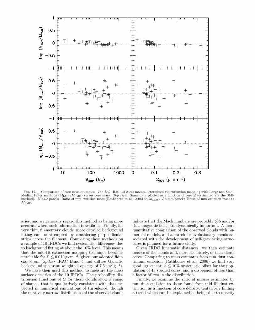
Fig. 12.— Comparison of core mass estimates. Top Left: Ratio of cores masses determined via extinction mapping with Large and SmallMedian Filter methods (MLMF/MSMF) versus core mass. Top right: Same data plotted as a function of core Σ (estimated via the SMFmethod). Middle panels: Ratio of mm emission mass (Rathborne et al. 2006) to MLMF. Bottom panels: Ratio of mm emission mass toMSMF.

aries, and we generally regard this method as being moreaccurate where such information is available. Finally, forvery thin, filamentary clouds, more detailed backgroundfitting can be attempted by considering perpendicularstrips across the filament. Comparing these methods ona sample of 10 IRDCs we find systematic differences dueto background fitting at about the 10% level. This meansthat the mid-IR extinction mapping technique becomesunreliable for Σ . 0.013 g cm−2 (given our adopted fidu-cial 8 µm [Spitzer IRAC Band 4 and diffuse Galacticbackground spectrum weighted] opacity of 7.5 cm2 g−1).

We have then used this method to measure the masssurface densities of the 10 IRDCs. The probability dis-tribution functions of Σ for these clouds show a rangeof shapes, that is qualitatively consistent with that ex-pected in numerical simulations of turbulence, thoughthe relatively narrow distributions of the observed clouds

indicate that the Mach numbers are probably . 5 and/orthat magnetic fields are dynamically important. A morequantitative comparison of the observed clouds with nu-merical models, and a search for evolutionary trends as-sociated with the development of self-gravitating struc-tures is planned for a future study.

Given IRDC kinematic distances, we then estimatemasses of the clouds and, more accurately, of their densecores. Comparing to mass estimates from mm dust con-tinuum emission (Rathborne et al. 2006) we find verygood agreement: a . 10% systematic offset for the pop-ulation of 43 studied cores, and a dispersion of less thana factor of two in the distribution.

Finally, we examine the ratio of masses estimated bymm dust emission to those found from mid-IR dust ex-tinction as a function of core density, tentatively findinga trend which can be explained as being due to opacity

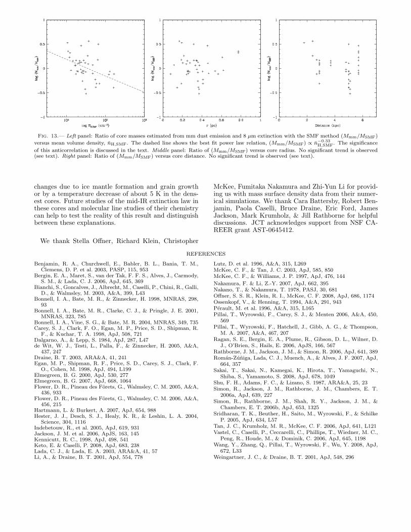
Fig. 13.— Left panel: Ratio of core masses estimated from mm dust emission and 8 µm extinction with the SMF method (Mmm/MSMF)

versus mean volume density, nH,SMF. The dashed line shows the best fit power law relation, (Mmm/MSMF) ∝ n−0.33H,SMF

. The significance

of this anticorrelation is discussed in the text. Middle panel: Ratio of (Mmm/MSMF) versus core radius. No significant trend is observed(see text). Right panel: Ratio of (Mmm/MSMF) versus core distance. No significant trend is observed (see text).

changes due to ice mantle formation and grain growthor by a temperature decrease of about 5 K in the dens-est cores. Future studies of the mid-IR extinction law inthese cores and molecular line studies of their chemistrycan help to test the reality of this result and distinguishbetween these explanations.

We thank Stella Offner, Richard Klein, Christopher

McKee, Fumitaka Nakamura and Zhi-Yun Li for provid-ing us with mass surface density data from their numer-ical simulations. We thank Cara Battersby, Robert Ben-jamin, Paola Caselli, Bruce Draine, Eric Ford, JamesJackson, Mark Krumholz, & Jill Rathborne for helpfuldiscussions. JCT acknowledges support from NSF CA-REER grant AST-0645412.

REFERENCES

Benjamin, R. A., Churchwell, E., Babler, B. L., Bania, T. M.,Clemens, D. P. et al. 2003, PASP, 115, 953

Bergin, E. A., Maret, S., van der Tak, F. F. S., Alves, J., Carmody,S. M., & Lada, C. J. 2006, ApJ, 645, 369

Bianchi, S., Goncalves, J., Albrecht, M., Caselli, P., Chini, R., Galli,D., & Walmsley, M. 2003, A&A, 399, L43

Bonnell, I. A., Bate, M. R., & Zinnecker, H. 1998, MNRAS, 298,93

Bonnell, I. A., Bate, M. R., Clarke, C. J., & Pringle, J. E. 2001,MNRAS, 323, 785

Bonnell, I. A., Vine, S. G., & Bate, M. R. 2004, MNRAS, 349, 735Carey, S. J., Clark, F. O., Egan, M. P., Price, S. D., Shipman, R.

F., & Kuchar, T. A. 1998, ApJ, 508, 721Dalgarno, A., & Lepp, S. 1984, ApJ, 287, L47de Wit, W. J., Testi, L., Palla, F., & Zinnecker, H. 2005, A&A,

437, 247Draine, B. T. 2003, ARA&A, 41, 241Egan, M. P., Shipman, R. F., Price, S. D., Carey, S. J., Clark, F.

O., Cohen, M. 1998, ApJ, 494, L199Elmegreen, B. G. 2000, ApJ, 530, 277Elmegreen, B. G. 2007, ApJ, 668, 1064Flower, D. R., Pineau des Forets, G., Walmsley, C. M. 2005, A&A,

436, 933Flower, D. R., Pineau des Forets, G., Walmsley, C. M. 2006, A&A,

456, 215Hartmann, L. & Burkert, A. 2007, ApJ, 654, 988Hester, J. J., Desch, S. J., Healy, K. R., & Leshin, L. A. 2004,

Science, 304, 1116Indebetouw, R., et al. 2005, ApJ, 619, 931Jackson, J. M. et al. 2006, ApJS, 163, 145Kennicutt, R. C., 1998, ApJ, 498, 541Keto, E. & Caselli, P. 2008, ApJ, 683, 238Lada, C. J., & Lada, E. A. 2003, ARA&A, 41, 57Li, A., & Draine, B. T. 2001, ApJ, 554, 778

Lutz, D. et al. 1996, A&A, 315, L269McKee, C. F., & Tan, J. C. 2003, ApJ, 585, 850McKee, C. F., & Williams, J. P. 1997, ApJ, 476, 144

Nakamura, F. & Li, Z.-Y. 2007, ApJ, 662, 395Nakano, T., & Nakamura, T. 1978, PASJ, 30, 681Offner, S. S. R., Klein, R. I., McKee, C. F. 2008, ApJ, 686, 1174Ossenkopf, V., & Henning, T. 1994, A&A, 291, 943Perault, M. et al. 1996, A&A, 315, L165Pillai, T., Wyrowski, F., Carey, S. J., & Menten 2006, A&A, 450,

569Pillai, T., Wyrowski, F., Hatchell, J., Gibb, A. G., & Thompson,

M. A. 2007, A&A, 467, 207Ragan, S. E., Bergin, E. A., Plume, R., Gibson, D. L., Wilner, D.

J., O’Brien, S., Hails, E. 2006, ApJS, 166, 567Rathborne, J. M., Jackson, J. M., & Simon, R. 2006, ApJ, 641, 389Roman-Zuniga, Lada, C. J., Muench, A., & Alves, J. F. 2007, ApJ,

664, 357Sakai, T., Sakai, N., Kamegai, K., Hirota, T., Yamaguchi, N.,

Shiba, S., Yamamoto, S. 2008, ApJ, 678, 1049Shu, F. H., Adams, F. C., & Lizano, S. 1987, ARA&A, 25, 23Simon, R., Jackson, J. M., Rathborne, J. M., Chambers, E. T.

2006a, ApJ, 639, 227Simon, R., Rathborne, J. M., Shah, R. Y., Jackson, J. M., &

Chambers, E. T. 2006b, ApJ, 653, 1325Sridharan, T. K., Beuther, H., Saito, M., Wyrowski, F., & Schilke

P. 2005, ApJ, 634, L57Tan, J. C., Krumholz, M. R., McKee, C. F. 2006, ApJ, 641, L121Vastel, C., Caselli, P., Ceccarelli, C., Phillips, T., Wiedner, M. C.,

Peng, R., Houde, M., & Dominik, C. 2006, ApJ, 645, 1198Wang, Y., Zhang, Q., Pillai, T., Wyrowski, F., Wu, Y. 2008, ApJ,

672, L33Weingartner, J. C., & Draine, B. T. 2001, ApJ, 548, 296

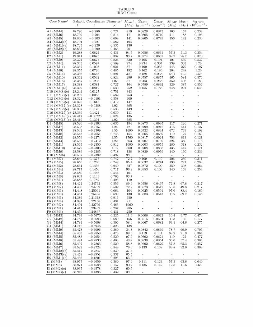
TABLE 3IRDC Cores

Core Namea Galactic Coordinates Diameterb Mmmc ΣLMF ΣSMF MLMF MSMF nH,SMF

l b (pc) (M⊙) (g cm−2) (g cm−2) (M⊙) (M⊙) (105cm−3)

A1 (MM4) 18.790 −0.286 0.721 219 0.0829 0.0813 163 157 0.232A2 (MM6) 18.799 −0.294 0.814 171 0.0805 0.0710 211 188 0.193A3 (MM5) 18.806 −0.303 0.698 141 0.0805 0.0749 156 142 0.230A4 (MM3)(e) 18.701 −0.227 0.582 194 - - - - -A5 (MM1)(e) 18.735 −0.226 0.535 736 - - - - -A6 (MM2)(e) 18.833 −0.299 0.465 201 - - - - -B1 (MM2) 19.288 0.0824 0.431 94.5 0.0656 0.0631 57.3 51.3 0.354B2 (MM1) 19.311 0.0675 0.337 93.7 0.0774 0.0687 32.2 25.7 0.370C1 (MM9) 28.324 0.0677 0.824 330 0.165 0.194 401 539 0.532C2 (MM4) 28.345 0.0597 0.509 274 0.234 0.304 239 303 1.26C3 (MM11) 28.352 0.1008 0.921 371 0.199 0.235 243 279 0.197C4 (MM6) 28.355 0.0726 0.485 192 0.162 0.186 204 248 1.20C5 (MM14) 28.356 0.0566 0.291 30.0 0.188 0.238 66.1 71.1 1.59C6 (MM10) 28.362 0.0532 0.824 296 0.0757 0.0857 465 584 0.576C7 (MM16) 28.367 0.1203 1.07 371 0.203 0.256 352 406 0.183C8 (MM17) 28.388 0.0381 0.727 164 0.0789 0.0892 329 387 0.556C9 (MM1)(e) 28.399 0.0812 0.630 952 0.155 0.183 248 291 0.643C10 (MM8)(e) 28.244 0.0127 0.751 343 - - - - -C11 (MM7)(e) 28.292 0.0065 0.582 253 - - - - -C12 (MM3)(e) 28.322 −0.0101 0.558 400 - - - - -C13 (MM5)(e) 28.325 0.1613 0.412 147 - - - - -C14 (MM12)(e) 28.328 −0.0388 1.02 395 - - - - -C15 (MM2)(e) 28.337 0.1170 0.533 449 - - - - -C16 (MM15)(e) 28.339 0.1424 0.630 111 - - - - -C17 (MM18)(e) 28.417 −0.00726 0.824 135 - - - - -C18 (MM13)(e) 28.419 0.1391 1.02 385 - - - - -D1 (MM5) 28.526 −0.2503 0.636 194 0.0873 0.0995 117 126 0.271D2 (MM7) 28.538 −0.2757 1.24 421 0.0799 0.0942 416 441 0.127D3 (MM3) 28.543 −0.2369 1.55 1690 0.0722 0.0844 672 729 0.108D4 (MM8) 28.543 −0.2651 0.746 154 0.0565 0.0669 119 127 0.169D5 (MM2) 28.559 −0.2274 1.55 1760 0.0817 0.0924 753 813 0.121D6 (MM4) 28.559 −0.2412 1.22 663 0.0707 0.0739 324 380 0.116D7 (MM1) 28.565 −0.2350 0.912 1000 0.0603 0.0655 280 318 0.232D8 (MM10) 28.579 −0.2303 1.13 360 0.0708 0.0836 435 447 0.171D9 (MM9) 28.589 −0.2285 0.718 138 0.0829 0.0959 140 160 0.239D10 (MM6) 28.557 −0.2382 0.497 98.6 - - - - -E1 (MM7) 28.644 0.1375 0.742 72.2 0.109 0.119 206 230 0.311E2 (MM5) 28.650 0.1260 0.742 85.4 0.0632 0.0774 193 221 0.298E3 (MM2) 28.661 0.1456 0.940 327 0.0872 0.100 359 398 0.264E4 (MM4) 28.717 0.1456 0.717 96.2 0.0953 0.106 140 169 0.254E5 (MM3) 28.580 0.1456 0.544 101 - - - - -E6 (MM6) 28.647 0.1143 0.766 93.7 - - - - -E7 (MM1) 28.688 0.1782 0.495 119 - - - - -F1 (MM8) 34.422 0.24792 0.556 89.6 0.0556 0.0497 72.8 67.8 0.217F2 (MM7) 34.438 0.24759 0.502 72.2 0.0573 0.0517 55.8 49.8 0.217F3 (MM6) 34.448 0.25091 0.664 104 0.0625 0.0591 97.0 88.4 0.166F4 (MM9) 34.454 0.25495 0.699 130 0.0583 0.0513 116 89.7 0.145F5 (MM5) 34.386 0.21378 0.915 550 - - - - -F6 (MM4) 34.394 0.22156 0.431 211 - - - - -F7 (MM2) 34.401 0.22709 0.466 1060 - - - - -F8 (MM1) 34.411 0.23489 0.287 985 - - - - -F9 (MM3) 34.459 0.24867 0.431 250 - - - - -G1 (MM3) 34.734 −0.5670 0.225 11.6 0.0606 0.0622 10.4 9.77 0.474G2 (MM2) 34.783 −0.5683 0.689 156 0.0515 0.0504 112 105 0.177G3 (MM4) 34.784 −0.5608 0.506 58.0 0.0667 0.0682 64.1 64.6 0.275G4 (MM1) 34.712 −0.5946 0.323 138 - - - - -H1 (MM9) 35.478 −0.3096 0.380 34.8 0.0842 0.0869 78.7 69.9 0.705H2 (MM4) 35.483 −0.2858 0.478 89.6 0.113 0.114 69.9 71.9 0.364H3 (MM5) 35.483 −0.2954 0.520 97.9 0.0602 0.0621 119 122 0.477H4 (MM8) 35.491 −0.2830 0.408 48.9 0.0830 0.0854 36.0 37.4 0.304H5 (MM6) 35.497 −0.2863 0.520 58.8 0.0602 0.0629 57.8 65.3 0.257H6 (MM7) 35.522 −0.2724 0.548 79.6 0.133 0.138 89.8 92.0 0.308H7 (MM2)(e) 35.417 −0.2847 0.239 37.3 - - - - -H8 (MM3)(e) 35.452 −0.2951 0.337 65.5 - - - - -H9 (MM1)(e) 35.456 −0.1801 0.295 63.0 - - - - -I1 (MM1) 38.957 −0.4659 0.380 97.0 0.111 0.124 57.3 63.6 0.640I2 (MM3) 38.971 −0.4588 0.157 9.12 0.135 0.142 12.8 11.6 1.65I3 (MM2)(e) 38.937 −0.4578 0.327 60.5 - - - - -I4 (MM4)(e) 38.949 −0.4385 0.432 39.8 - - - - -

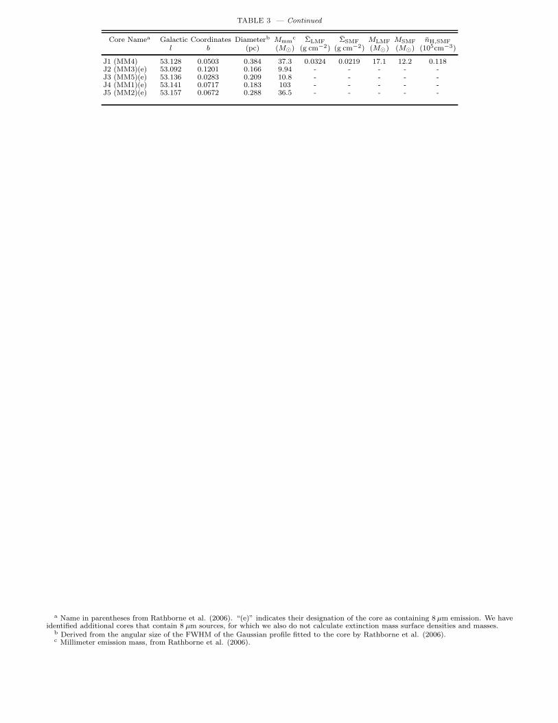
TABLE 3 — Continued

Core Namea Galactic Coordinates Diameterb Mmmc ΣLMF ΣSMF MLMF MSMF nH,SMF

l b (pc) (M⊙) (g cm−2) (g cm−2) (M⊙) (M⊙) (105cm−3)

J1 (MM4) 53.128 0.0503 0.384 37.3 0.0324 0.0219 17.1 12.2 0.118J2 (MM3)(e) 53.092 0.1201 0.166 9.94 - - - - -J3 (MM5)(e) 53.136 0.0283 0.209 10.8 - - - - -J4 (MM1)(e) 53.141 0.0717 0.183 103 - - - - -J5 (MM2)(e) 53.157 0.0672 0.288 36.5 - - - - -

a Name in parentheses from Rathborne et al. (2006). “(e)” indicates their designation of the core as containing 8 µm emission. We haveidentified additional cores that contain 8 µm sources, for which we also do not calculate extinction mass surface densities and masses.

b Derived from the angular size of the FWHM of the Gaussian profile fitted to the core by Rathborne et al. (2006).c Millimeter emission mass, from Rathborne et al. (2006).