Modelling flood levels associated with ice consolidation events triggered by upstream ice

jam release waves in the Hay River Delta, NWT

by

Michael De Coste

A thesis submitted in partial fulfillment of the requirements for the degree of

Master of Science

In

Water Resources Engineering

Department of Civil and Environmental Engineering

University of Alberta

© Michael De Coste, 2017

ii

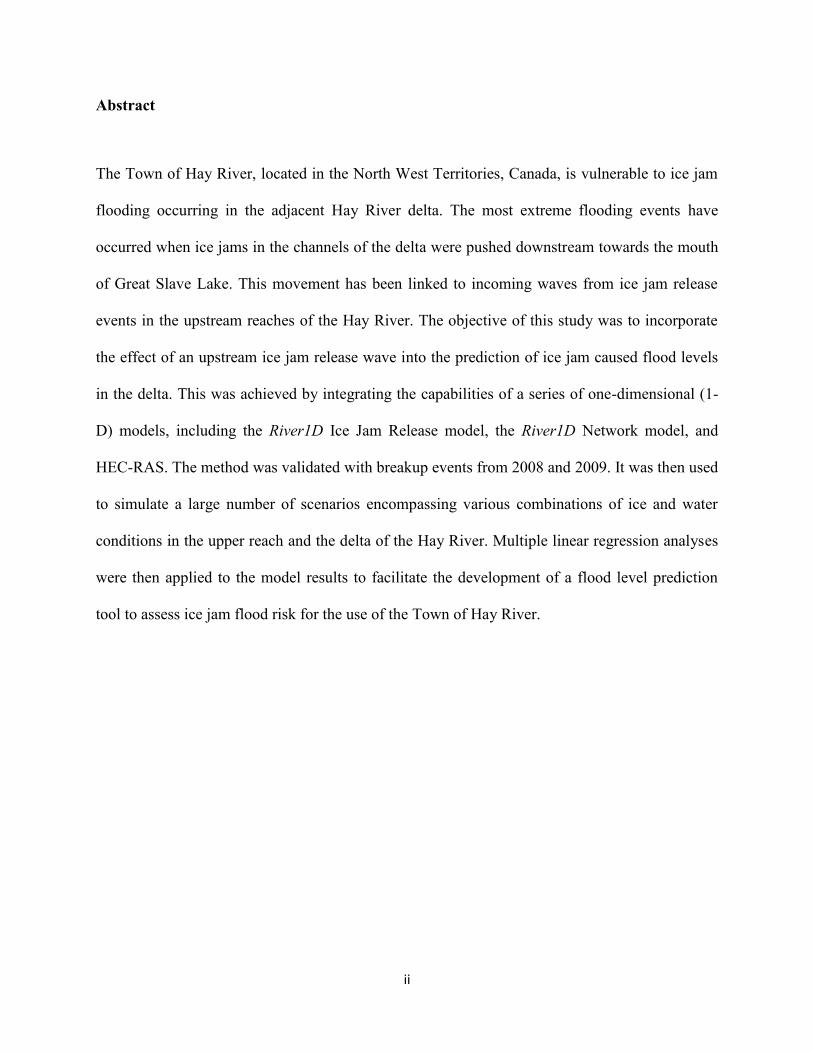
Abstract

The Town of Hay River, located in the North West Territories, Canada, is vulnerable to ice jam

flooding occurring in the adjacent Hay River delta. The most extreme flooding events have

occurred when ice jams in the channels of the delta were pushed downstream towards the mouth

of Great Slave Lake. This movement has been linked to incoming waves from ice jam release

events in the upstream reaches of the Hay River. The objective of this study was to incorporate

the effect of an upstream ice jam release wave into the prediction of ice jam caused flood levels

in the delta. This was achieved by integrating the capabilities of a series of one-dimensional (1-

D) models, including the River1D Ice Jam Release model, the River1D Network model, and

HEC-RAS. The method was validated with breakup events from 2008 and 2009. It was then used

to simulate a large number of scenarios encompassing various combinations of ice and water

conditions in the upper reach and the delta of the Hay River. Multiple linear regression analyses

were then applied to the model results to facilitate the development of a flood level prediction

tool to assess ice jam flood risk for the use of the Town of Hay River.

iii

Acknowledgments

The author would like to extend his thanks to his supervisor, Dr. Yuntong She, for her constant

guidance and support throughout this project, which is deeply appreciated. Thank you as well to

Dr. Mark Loewen and Dr. Wei Liu for being a part of the examining committee.

Thanks are also extended to the University of Alberta’s River Ice Research Group, in particular

Dr. Faye Hicks and Julia Blackburn for their assistance and guidance.

This research was funded through a grant from the Natural Sciences and Engineering Research

Council of Canada which is gratefully acknowledged.

The author would also like to extend thanks to his family and friends for their guidance and

support throughout this research.

iv

Table of Contents

Chapter 1 : Introduction .............................................................................................................. 1

1.1 Background ........................................................................................................................... 1

1.2 Previous Research ................................................................................................................. 2

1.3 Study Objectives ................................................................................................................... 5

Chapter 2 : Methodology............................................................................................................ 11

2.1 Study Reach Description ..................................................................................................... 11

2.2 Model Description and Setup .............................................................................................. 11

2.2.1 River1D Ice Jam Release Model .................................................................................. 11

2.2.2 River1D Network Model .............................................................................................. 15

2.2.3 HEC-RAS ..................................................................................................................... 18

2.3 Integrated Modelling Method.............................................................................................. 19

2.4 Modelling Domain .............................................................................................................. 20

Chapter 3 : Calibration and Validation .................................................................................... 26

3.1 Validation of River1D Network Model ............................................................................... 26

3.2 Breakup Modelling .............................................................................................................. 27

3.2.1 2008 Breakup ................................................................................................................ 28

3.2.2 2009 Breakup ................................................................................................................ 30

Chapter 4 : Model Application .................................................................................................. 43

4.1 Hypothetical Scenarios ........................................................................................................ 43

v

4.2 Multiple Linear Regression (MLR) Analyses ..................................................................... 48

4.3 Flood Level Prediction Tool ............................................................................................... 57

Chapter 5 : Summary and Conclusions .................................................................................... 71

References .................................................................................................................................... 73

Appendix A: Matlab Code of the Flood Level Prediction Tool .............................................. 76

vi

List of Tables

Table 3.1 Comparison of modelled flow splits to 2007 ADCP measurements. ........................... 27

Table 4.1 List of documented historical ice jam events in the upstream reaches of the Hay River.

........................................................................................................................................... 45

Table 4.2 List of documented historical ice jams in the Hay River Delta. ................................... 47

Table 4.3 Selected values of key variables in the simulated hypothetical events. ........................ 48

Table 4.4 List of MLR equations for each location in the East Channel of the Hay River Delta. 50

Table 4.5 Rankings of the five key variables. ............................................................................... 53

Table 4.6 Range of modelled top of ice elevations at key locations in the East Channel of the

Hay River Delta. ................................................................................................................ 54

Table 4.7 List of rankd MLR equations in the East Channel of the Hay River Delta. ................. 55

vii

List of Figures

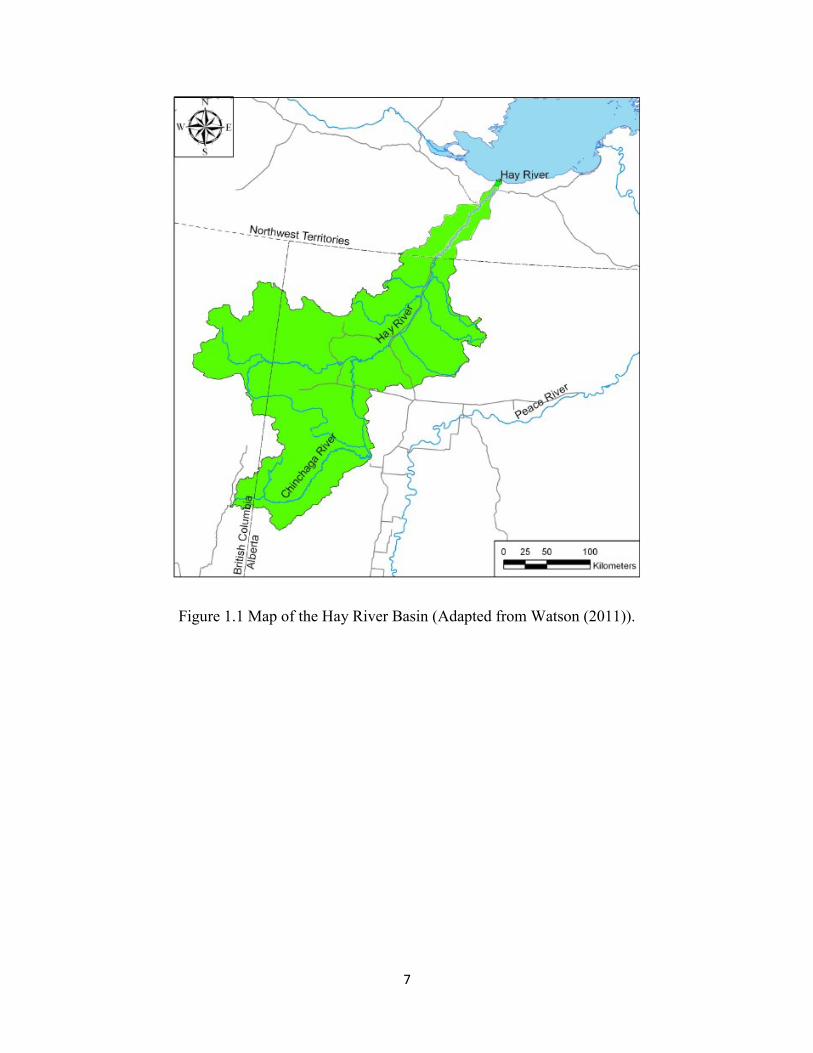
Figure 1.1 Map of the Hay River Basin (Adapted from Watson (2011)). ...................................... 7

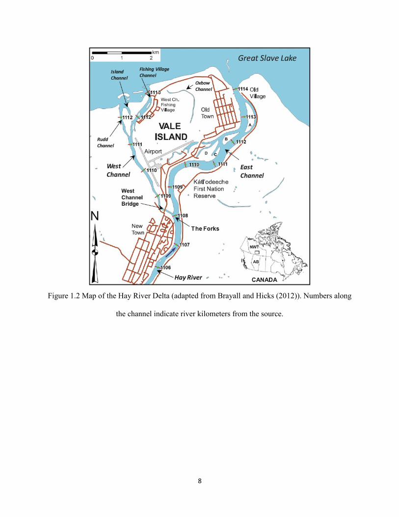
Figure 1.2 Map of the Hay River Delta (adapted from Brayall and Hicks (2012)). Numbers along

the channel indicate river kilometers from the source. ....................................................... 8

Figure 1.3 2008 Ice Jam Flood in the East Channel of the Hay River Delta (University of Alberta

River Ice Research Group). ................................................................................................. 9

Figure 1.4 2008 Ice Jam Flooding in the Old Town District of the Town of Hay River

(University of Alberta River Ice Research Group). .......................................................... 10

Figure 2.1 Bed profile of equivalent rectangular channel for the Hay River showing key

landmarks and gauge stations (Adapted from Hicks et al., 1992). ................................... 22

Figure 2.2 Open channel junction configurations for (a) combing junction and (b) dividing

junction (adapted from Shabayek 2002). .......................................................................... 23

Figure 2.3 Flowchart of integrated modelling method. ................................................................ 24

Figure 2.4 Plan view schematic of River1D Network model geometry of Hay River Delta. ...... 25

Figure 3.1 Locations of ADCP cross sections in the Hay River Delta (Brayall 2011). ................ 33

Figure 3.2 Comparison of flow apportionment into East Channel between River1D Network

model and River2D (Brayall and Hicks, 2012). ................................................................ 34

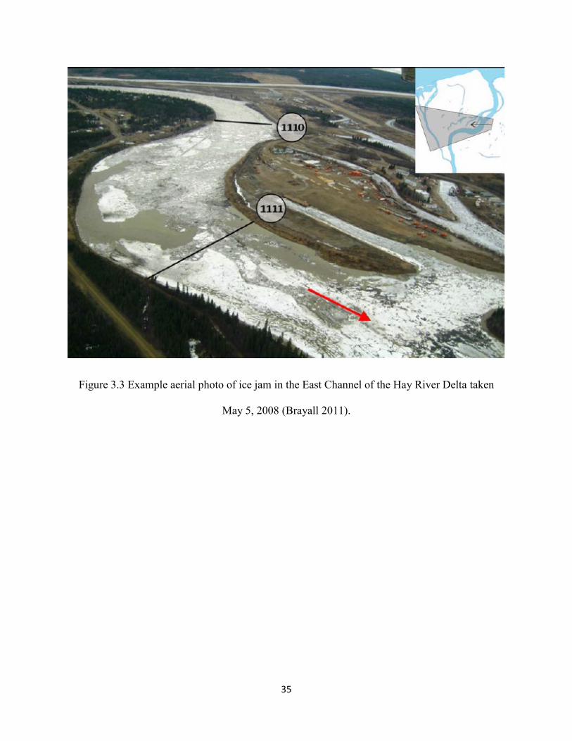
Figure 3.3 Example aerial photo of ice jam in the East Channel of the Hay River Delta taken

May 5, 2008 (Brayall 2011). ............................................................................................. 35

viii

Figure 3.4 Calibration of 2008 upstream ice jam using data from WSC Hay River near Hay River

and EMO gauge at Pine Point Bridge. .............................................................................. 36

Figure 3.5 Ice Jam Map for modelled 2008 release (adapted from Hicks et al., 1992). ............... 36

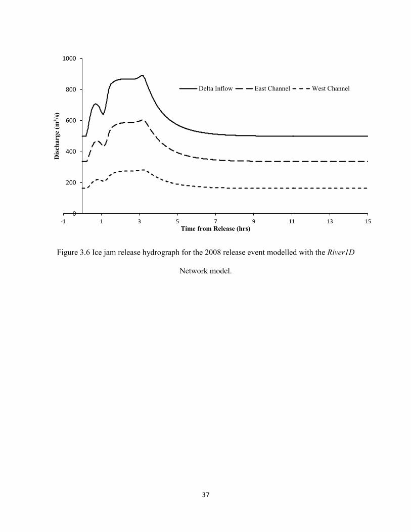
Figure 3.6 Ice jam release hydrograph for the 2008 release event modelled with the River1D

Network model. ................................................................................................................. 37

Figure 3.7 Pre a) and post b) wave delta ice jam configurations for East Channel-2008. ............ 38

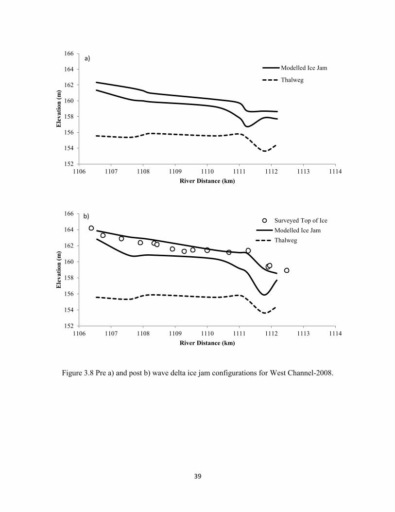
Figure 3.8 Pre a) and post b) wave delta ice jam configurations for West Channel-2008. .......... 39

Figure 3.9 Ice Jam Map for modelled 2009 release (adapted from Hicks et al., 1992). ............... 40

Figure 3.10 Ice jam release hydrograph for the 2009 release event modelled with the River1D

Network model. ................................................................................................................. 40

Figure 3.11 Pre (a) and post b) wave delta ice jam configurations for East Channel-2009. ........ 41

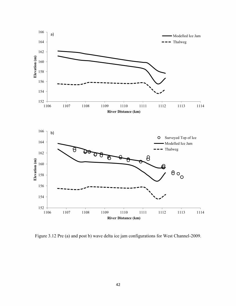
Figure 3.12 Pre (a) and post b) wave delta ice jam configurations for West Channel-2009. ....... 42

Figure 4.1 Comparison between the predicted and the simulated top of ice level at Km 1108.3 for

the two regression methods: a) without rank and b) with rank. ........................................ 59

Figure 4.2 Comparison between the predicted and the simulated top of ice level at Km 1109 for

the two regression methods: a) without rank and b) with rank. ........................................ 60

Figure 4.3 Comparison between the predicted and the simulated top of ice level at Km 1109.5 for

the two regression methods: a) without rank and b) with rank. ........................................ 61

ix

Figure 4.4 Comparison between the predicted and the simulated top of ice level at Km 1109.98

for the two regression methods: a) without rank and b) with rank. .................................. 62

Figure 4.5 Comparison between the predicted and the simulated top of ice level at Km 1111 for

the two regression methods: a) without rank and b) with rank. ........................................ 63

Figure 4.6 Comparison between the predicted and the simulated top of ice level at Km 1111.55

for the two regression methods: a) without rank and b) with rank. .................................. 64

Figure 4.7 Comparison between the predicted and the simulated top of ice level at Km 1112.2 for

the two regression methods: a) without rank and b) with rank. ........................................ 65

Figure 4.8 Comparison between the predicted and the simulated top of ice level at Km 1112.4 for

the two regression methods: a) without rank and b) with rank. ........................................ 66

Figure 4.9 Comparison between the predicted and the simulated top of ice level at Km 1113.22

for the two regression methods: a) without rank and b) with rank. .................................. 67

Figure 4.10 Comparison between the predicted and the simulated top of ice level at Km 1113.61

for the two regression methods: a) without rank and b) with rank. .................................. 68

Figure 4.11 Comparison of the top of ice level predicted by the proposed tool, the IJPG and the

observation for the 1992 flooding event. .......................................................................... 69

Figure 4.12 Comparison of the top of ice level predicted by the proposed tool, the IJPG and the

key landmarks for the 2007 flooding event....................................................................... 70

x

List of Symbols

A = the total area of the cross-section under the water surface (m2)

Aw = cross-sectional area of the water, perpendicular to the flow (m2)

a1 = velocity weighing coefficient of the main channel (dimensionless)

a2 = velocity weighing coefficient of the lateral channel (dimensionless)

aj (j = 1, 6) = regression coefficients (dimensionless)

B = width of the ice accumulation (m)

bj (j = 1, 6) = ranked regression coefficients (dimensionless)

Cf = cohesion (Pa)

C* = the nondimensional Chezy’s coefficient (dimensionless)

e = porosity of the ice accumulation (dimensionless)

g = acceleration due to gravity (m2/s)

H = the depth of flow under the water surface (m)

Hw = depth of water flow (m)

he = energy head loss (m)

Kx = a passive pressure coefficient (dimensionless)

Lj = length of the upstream jam (km)

LL = lake level (m)

xi

L1= the length of the main channel control volume (m)

L2 = the length of the lateral channel control volume (m)

n = Manning’s resistance coefficients of the channel bed (dimensionless)

Q = the total discharge, including both water and ice flow (m3/s)

Qc = carrier discharge of upstream jam (m3/s)

Qw = water discharge (m3/s)

R = hydraulic radius (m)

S = stream slope (dimensionless)

SC = the total rank of the scenario predicted by the multiple linear regression equation

(dimensionless)

Sf = friction slope determined using Manning’s equation (dimensionless)

SL = the rank for the length of the upstream jam (dimensionless)

SQ = the rank for carrier discharge (dimensionless)

SS = the rank for toe shift of the delta jam (dimensionless)

ST = the rank for the toe location of the upstream jam (dimensionless)

SWL = the rank for the lake level (dimensionless)

So = river bed slope (dimensionless)

TOI = simulated top of ice levels in the delta region (m)

xii

TS = toe shift of the delta jam (km)

Tj = toe location of upstream jam (km)

ti = thickness of the ice jam accumulation (m)

V = ice and water velocity (m/s)

Vw = velocity of water flow (m/s)

V1= average velocity of main channel (m/s)

V2 = average velocities of lateral channel (m/s)

x = longitudinal co-ordinate (m)

Y1=depth of water at the cross section of lateral channel (m)

Y2=depth of water at the cross section of main channel (m)

Z1=elevation of the main channel invert (m)

Z2=elevation of the lateral channel invert (m)

ρ = density of water (kg/m3)

ρi= density of ice (kg/m3)

τ = shear stress of flow on underside of accumulation (Pa)

𝜆1 = an empirically determined coefficient approximating bank resistance effects on the ice run

(dimensionless)

xiii

𝜆2 = an empirical coefficient accounting for the longitudinal dispersion of the released ice mass

(dimensionless)

ϕ = angle of internal friction of the ice accumulation (°)

ξ = QWB/QWA is a discharge ratio;

xiv

List of Abbreviations

AB=Alberta

ADCP=Acoustic Doppler Current Profiler

BC=British Columbia

CDG=Characteristic-Dissipative-Galerkin

EMO=Emergency Measures Organization

IJPG=Ice Jam Profile Generator

MLR=Multiple Linear Regression

NWT=North West Territories

TOI=Top of Ice

WSC=Water survey of Canada

U of A=University of Alberta

1

Chapter 1 : Introduction

1.1 Background

Dynamic breakup is a critical event in many northern rivers. High flows resulting from

spring snowmelt runoff lift an existing ice cover out of place, break it, and carry it downstream.

An ice jam can form when this broken ice becomes blocked in the channel upon entering

constrictions or flowing into intact ice cover. Flooding often results from significant flow

obstructions or from the release of ice jams creating waves of water and ice. Ice jam caused

flooding can occur incredibly fast, potentially leaving nearby communities with little notice and

creating challenges in accurately predicting both the severity and timing of such events.

The Hay River originates in British Columbia (BC) and flowing through northern Alberta

(AB) into the North West Territories (NWT), as shown in Figure 1.1. Due to its north flowing

nature and a steep reach containing two waterfalls, dynamic breakup occurs almost yearly. The

general pattern of breakup progression has been found to be relatively consistent from year to

year (Kovachis et al., 2010). Breakup begins with melting in the headwaters of the southern

portion of the basin. This snowmelt runoff lifts and break the ice cover, carrying it downstream

to create a series of ice jams throughout the upstream reaches of the river. These ice jams can

release sending a wave traveling downstream towards the Hay River Delta, where the Town of

Hay River is located.

The entrance of the Hay River Delta is known as the Forks (km 1108), a location where

the Hay River splits into the East Channel and the West Channel. These channels flow around

Vale Island, the location of the Old Town district. The “New Town,” located upstream of the

delta in an area less prone to flooding, was established after a particularly severe flood that

2

occurred in 1963. The delta region is also home to several fishing villages, including the West

Point Fishing Village on the east side of the West Channel, as well as the Katl’odeeche First

Nations Reserve on the east side of the East Channel. Figure 1.2 shows a detailed map of the Hay

River delta.

At the onset of breakup, small ice accumulations form within the delta. The arrival of the

upstream ice jam release waves causes great increase in discharge and brings large amount of

additional ice. Thus, the small accumulations within the delta consolidate, becoming much

longer and thicker ice jams. The arrival of the wave also pushes the toe of the delta jams

downstream towards the mouth of the river, which has been witnessed in 1965, 1978, 1985,

1989, 1992, and 2007. In these instances, flooding resulted on Vale Island. In 2008, severe

flooding occurred in the Hay River Delta when an ice jam in the East Channel was pushed

further downstream by an incoming release wave. Figure 1.3 shows this flood in the upstream

region of the East Channel and Figure 1.4 shows the extent of the flooding in the Old Town

district. This flood resulted in the declaration of a state of emergency for the Town of Hay River

and over one million dollars in damages. Minor flooding has also occurred in 2009 and 2010 as a

result of ice jam shifting in the delta. Therefore, the direct effects of ice jam release waves on the

conditions of ice jams in the delta are a vital component of developing a flood evacuation plan

for the community.

1.2 Previous Research

Studies have been focusing on predicting ice jam caused flooding in the Hay River Delta

through computer modelling. Gerard and Stanley (1988) developed a first generation flood

forecast procedure based around historical flow data. This procedure was limited by the

3

unpredictable nature of jam shifting in the delta and the difficulty in estimating the timing and

magnitude of ice jam release waves from upstream. Gerard and Jasek (1989) further evaluated

this procedure, recommending flood mitigation techniques for the West Channel, additional

measurements in the East Channel, and adaptation of the model developed into a computer based

format. Gerard et al. (1990) utilised unsteady flow analysis to evaluate flow waves caused by

upstream ice jam releases. The models ability to capture wave travel times and peak discharges

was limited, due to a lack of field data on flood surges in the Hay River to use in refining the

model’s equations. Hicks et al. (1992) modelled ice jam release waves on the Hay River using

the cdg1-D model (the precursor to River1D), and the resulting peak flows at the delta were used

together with the ICEJAM model (Flato and Gerard, 1986) to estimate expected ice jam flood

levels in the Town. At that time, no data was available on ice jam release events on the Hay

River, so the initial ice jam profiles were estimated using an equilibrium ice jam approximation

to estimate worst-case scenarios, and a suite of hypothetical ice jam release events were modeled

to give a range of possible outcomes.

She and Hicks (2005) later enhanced the cdg1-D model to add the calculation of actual

ice jam profiles for release, based on the same algorithm used in the ICEJAM model, calling it

the River1D model. Watson (2011) applied this updated model to multiple ice jam release events

documented on the Hay River from the monitoring program during the years 2007-2009. The

monitoring program consisted of remote water level monitoring at four sites along the Hay

River, as well as time lapse cameras and aerial reconnaissance flights. This enabled a detailed

overview and timeline of the breakup progress of these years, with observations of the movement

of waves through the Hay River obtained. It was found that the model accurately reproduced the

4

timing and severity of the release wave in comparison to measurements taking at stations along

the Hay River.

Brayall and Hicks (2012) utilised the University of Alberta’s (U of A) two-dimensional

(2-D) numerical model River2D to simulate the flood levels resulting from ice jam consolidation

events caused by incoming waves. This study involved the use of a summer survey to obtain the

bathymetry of the Hay River Delta, as well as observations taken during both freeze up and

breakup to better understand winter conditions and verify the accuracy of the model in depicting

the breakup events. 11 ice jam profiles were modelled. The model results were used to develop

an ‘ice jam profile generator’ (IJPG) to predict the expected flood levels at key locations in the

town, using peak discharge estimates from the River1D model as input. Although this dual-

model flood forecasting system is effective for predicting expected ice jam flood levels, it has

three key limitations. First, the 2-D modelling process was considered time and labor intensive,

making it difficult to apply to other sites. The transverse variations within individual channels

provided by the 2-D model are not the highest concern in flood forecasting. Second, the resulting

profile generator does not explicitly include movement of the ice jam toe in the delta during

consolidation events, but instead relies on the ‘typical’ locations of these ice jam toes in the past.

Third, the IJPG assumes that all incoming ice jam release waves to the Town will cause an ice

jam consolidation (shoving) event; however, this does not always happen.

Zhao (2011) demonstrated the potential of using fuzzy logic and artificial neural

networks to forecast breakup timing and severity for the Town of Hay River. A system of input

variables was identified for these systems with both long and short lead times, including

accumulated degree days of freezing and thawing, ice thickness, water levels on the days of

freeze up onset and onset of water rise, accumulated rainfall and snowfall, and peak discharge.

5

The study also showed that the peak discharge caused by an upstream ice jam release event was

an important factor affecting the ice jam flood severity in the delta.

1.3 Study Objectives

This study consisted of two objectives: (1) to incorporate the effects of upstream ice jam

release waves in the prediction of ice jam flood levels within the Hay River Delta and explicitly

include the effect of jam toe shifting during consolidation events, and (2) to investigate the

possibility of using 1-D network modelling to provide an operational tool for flood forecasting.

To achieve these objectives three separate models were applied sequentially and iteratively: (1)

the updated University of Alberta’s River1D Ice Jam Release model (She and Hicks, 2006),

which includes consideration of ice effects, was used for simulating the ice jam release events,

(2) the new University of Alberta’s River1D Network model (Blackburn et al., 2015) was used

for simulating wave propagation in the multi-channel network, and (3) the US Army Corps of

Engineers HEC-RAS model was used for simulating the ice jam profiles within the individual

delta channels. Data previously gathered from the extensive field program in the Hay River

region was used to calibrate and validate the new integrated modelling method. The validated

method was then utilised to simulate a series hypothetical scenarios and the results were used in

the development of a flood level prediction tool.

This thesis details how the objectives of this study were achieved. Chapter 2 describes the

study reach, the utilised hydrodynamic models, and the integrated modelling method. Chapter 3

describes the validation of the proposed method. Chapter 4 then discusses the large set of

hypothetical modelling scenarios that the methodology was applied to. The rationale behind the

selection of these scenarios is also detailed. Following this, the methods of statistical analysis

6

used in interpreting the obtained data are summarized, with the description of the final flood

level prediction tool and its validation then detailed.

7

Figure 1.1 Map of the Hay River Basin (Adapted from Watson (2011)).

8

Figure 1.2 Map of the Hay River Delta (adapted from Brayall and Hicks (2012)). Numbers along

the channel indicate river kilometers from the source.

9

Figure 1.3 2008 Ice Jam Flood in the East Channel of the Hay River Delta (University of Alberta

River Ice Research Group).

10

Figure 1.4 2008 Ice Jam Flooding in the Old Town District of the Town of Hay River

(University of Alberta River Ice Research Group).

11

Chapter 2 : Methodology

2.1 Study Reach Description

The relevant reach of the Hay River extends from the boundary between the NWT and

AB border at river station km 945.17 to Great Slave Lake at km 1114.24. The bed profile of this

reach was previously determined by Gerard et al., 1990 and Hicks et al., 1992, averaged within

five sub-reaches (Figure 2.1). River stations were measured from the origin of the river. The

upper part of the study reach is relatively flat with an average slope of 0.0002. The region

between km 1034 to km 1048 includes the Alexandra Falls (km 1034), the Louise Falls (km

1037.1), and a very steep gorge section. The average slope is 0.0058. Downstream of km 1048

extending to the entrance of the delta at km 1108, the bank height gradually decreases and the

slope of the river reduces to an average of 0.0005. Ice jams frequently form in this region and

their releases have been linked to severe delta flooding (Gerard and Stanley, 1988). At km 1108,

the river splits and forms the delta with an average slope of 0.0001. The gauge stations used for

calibration or as boundary conditions in this study are also shown, including the Water Survey of

Canada (WSC) gauges of Hay River near NWT/AB border (km 945.5), near Hay River (km

1095) and at Great Slave Lake (km 1114.24), as well as the Emergency Measures Organization

(EMO) at Alexandra Fall (km 1035) and Pine Point Bridge (km 1098).

2.2 Model Description and Setup

2.2.1 River1D Ice Jam Release Model

The first component of the proposed modelling method utilised in this research is the

River1D Ice Jam Release model (She and Hicks, 2006). This model was built upon the public

domain River1D software employing a characteristic-dissipative-Galerkin (CDG) finite element

scheme (Hicks and Steffler, 1992). It is capable of simulating unimpeded ice jam release wave

12

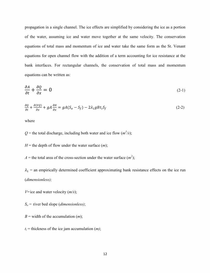
propagation in a single channel. The ice effects are simplified by considering the ice as a portion

of the water, assuming ice and water move together at the same velocity. The conservation

equations of total mass and momentum of ice and water take the same form as the St. Venant

equations for open channel flow with the addition of a term accounting for ice resistance at the

bank interfaces. For rectangular channels, the conservation of total mass and momentum

equations can be written as:

𝜕𝐴

𝜕𝑡+

𝜕𝑄

𝜕𝑥= 0 (2-1)

𝜕𝑄

𝜕𝑡+

𝜕(𝑉𝑄)

𝜕𝑥+ 𝑔𝐴

𝜕𝐻

𝜕𝑥= 𝑔𝐴(𝑆𝑜 − 𝑆𝑓) − 2𝜆1𝑔𝐵𝑡𝑖𝑆𝑓 (2-2)

where

Q = the total discharge, including both water and ice flow (m3/s);

H = the depth of flow under the water surface (m);

A = the total area of the cross-section under the water surface (m2);

𝜆1 = an empirically determined coefficient approximating bank resistance effects on the ice run

(dimensionless);

V=ice and water velocity (m/s);

So = river bed slope (dimensionless);

B = width of the accumulation (m);

ti = thickness of the ice jam accumulation (m);

13

Sf = friction slope determined using Manning’s equation (dimensionless):

34

2

R

VVnS f

(2-3)

n = Manning’s resistance coefficients of the channel bed (dimensionless);

R = hydraulic radius (m);

Equations (2-1) and (2-2) are solved in an uncoupled sequence with the ice mass continuity

equation:

𝜕𝑡𝑖

𝜕𝑡+

𝜕(𝑉𝑡𝑖)

𝜕𝑥+

𝑉𝑡𝑖

𝐵

𝑑𝐵

𝑑𝑥= 𝜆2

𝜕2𝑡𝑖

𝜕𝑥2 (2-4)

where 𝜆2 is another empirical coefficient accounting for the longitudinal dispersion of the

released ice mass. This parameter, together with 𝜆1, is used to empirically approximate the full

ice dynamics.

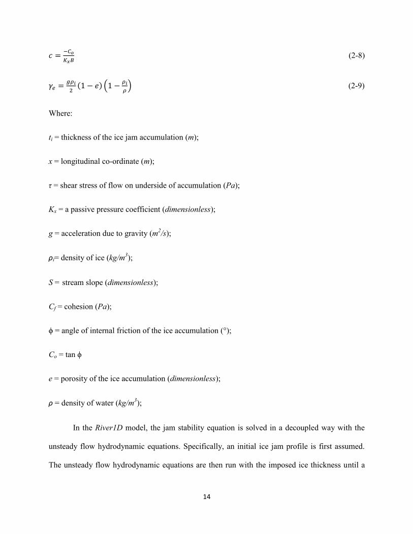
To make it convenient to simulate ice jam release events, the ice jam stability equation (Pariset et

al., 1966; Uzuner and Kennedy, 1976) was also incorporated into the model to calculate the

initial steady state ice jam profile prior to release.

𝑡𝑖𝜕𝑡𝑖

𝜕𝑥= 𝑎 + 𝑏𝑡𝑖 + 𝑐𝑡𝑖

2 (2-5)

in which:

𝑎 =𝜏

2𝐾𝑥𝛾𝑒 (2-6)

𝑏 =𝑔𝜌𝑖𝑆−(

2𝐶𝑓𝐵

⁄ )

2𝐾𝑥𝛾𝑒 (2-7)

14

𝑐 =−𝐶𝑜

𝐾𝑥𝐵 (2-8)

𝛾𝑒 =𝑔𝜌𝑖

2(1 − 𝑒) (1 −

𝜌𝑖

𝜌) (2-9)

Where:

ti = thickness of the ice jam accumulation (m);

x = longitudinal co-ordinate (m);

τ = shear stress of flow on underside of accumulation (Pa);

Kx = a passive pressure coefficient (dimensionless);

g = acceleration due to gravity (m2/s);

ρi= density of ice (kg/m3);

S = stream slope (dimensionless);

Cf = cohesion (Pa);

ϕ = angle of internal friction of the ice accumulation (°);

Co = tan ϕ

e = porosity of the ice accumulation (dimensionless);

ρ = density of water (kg/m3);

In the River1D model, the jam stability equation is solved in a decoupled way with the

unsteady flow hydrodynamic equations. Specifically, an initial ice jam profile is first assumed.

The unsteady flow hydrodynamic equations are then run with the imposed ice thickness until a

15

steady state is reached. Based on the new steady state solution, a new ice jam profile is

calculated. These steps are repeated until the change in the computed ice jam profile and

hydrodynamic condition is within a specified tolerance.

2.2.2 River1D Network Model

The second model utilised in the proposed method is the River1D Network model, also

built upon the River1D software. It models wave propagation in channel networks under both

open water and intact (non-moving) ice cover conditions. It does not assume equal energy or

equal water levels at the junction, as is the case in many other 1-D network models. The model

accounts for significant physical effects at junctions such as gravity forces and channel resistance

which are critical for modelling dynamic wave propagation. These effects are particularly

important in river deltas due to the largeness of horizontal scale relative to the vertical scale

(Blackburn et al., 2015). Therefore, the model is essential for this study, as the capability to

model highly dynamic ice jam release waves through the Hay River Delta is required.

In open channel networks, the individual channel reaches are connected through junctions.

The Network model solves the conservation of mass and momentum equations in both single

channels and at the junctions. In rectangular single channels, the 1-D conservation of mass and

momentum takes the form of the St. Venant equations:

𝜕𝐴𝑤

𝜕𝑡+

𝜕𝑄𝑤

𝜕𝑥= 0 (2-10)

𝜕𝑄𝑤

𝜕𝑡+

𝜕(𝑉𝑤𝑄𝑤)

𝜕𝑥+ 𝑔𝐴𝑤

𝜕𝐻𝑤

𝜕𝑥= 𝑔𝐴𝑤(𝑆𝑜 − 𝑆𝑓) (2-11)

where:

Aw = cross-sectional area of the water, perpendicular to the flow (m2);

16

Hw = depth of water flow (m);

Qw = water discharge (m3/s);

Vw = velocity of water flow (m2/s);

All other variables are as previously defined.

The equations at the junctions are based on the theoretical study conducted by Shabayek

(2002). These junctions consist of three individual channels, arranged in configurations which

are considered combining or dividing. Rectangular channel geometry is considered and the

layouts of these junctions are illustrated in Figure 2.2. In a combining junction (Figure 2.2a),

subscript A and C indicate the sections in the main channel just upstream and downstream of the

junction, while subscript B indicates the section of the lateral channel just upstream of the

junction. The flow variables to be evaluated are the water depth and discharge at these three

sections. Two control volumes, one for the main channel and one for the lateral channel, are

considered and each has a conservation of momentum equation (Shabayek, 2002). For the main

channel control volume:

−𝜌𝑄𝑊𝐶𝑉𝑊𝐶 + 𝜌𝑄𝑊𝐶𝑉𝑊𝐴 =𝛾𝐻𝑊𝐶

2

2𝐵𝐶 −

𝛾𝐻𝑊𝐴2

2𝐵𝐴(1 − 𝜉) +

𝛾

2(

𝐻𝑊𝐶+𝐻𝑊𝐵

2)

2(𝐵𝐴(1 − 𝜉) − 𝐵𝐶) +

𝛾 (𝐻𝑊𝐶𝐵𝐶+𝐻𝑊𝐴𝐵𝐴(1−𝜉)

2) 𝐿1𝑆𝑜 − 𝜌 (

𝑉𝑊𝐴2

𝐶∗) (𝐵𝐴(1 − 𝜉) + 𝑦𝐴)𝐿1 (2-12)

and for the lateral channel control volume:

−𝜌𝑄𝑊𝐵𝑉𝑊𝐵 + 𝜌𝑄𝑊𝐵𝑉𝑊𝐴 =𝛾𝐻𝑊𝐵

2

2𝐵𝐵 −

𝛾𝐻𝑊𝐴2

2𝐵𝐴𝜉 +

𝛾

2(

𝐻𝑊𝐶+𝐻𝑊𝐵

2)

2(𝐵𝐴𝜉 − 𝐵𝐵) +

𝛾 (𝐻𝑊𝐵𝐵𝐵+𝐻𝑊𝐴𝐵𝐴𝜉

2) 𝐿2𝑆𝑜 − 𝜌 (

𝑉𝑊𝐴2

𝐶∗) (𝐵𝐴𝜉 + 𝑦𝐴)𝐿2 (2-13)

17

where:

ξ = QWB/QWA is a discharge ratio;

L1= the length of the main channel control volume (m);

L2 = the length of the lateral channel control volume (m);

C* = the nondimensional Chezy’s coefficient;

With the other variables as defined in Figure 2.2a. The interfacial shear force, the separation

zone shear force, and the centrifugal effects which were accounted for in Shabayek (2002)’s

theoretical model are neglected in the current version of the model.

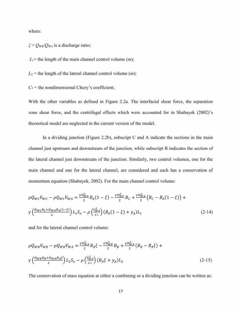
In a dividing junction (Figure 2.2b), subscript C and A indicate the sections in the main

channel just upstream and downstream of the junction, while subscript B indicates the section of

the lateral channel just downstream of the junction. Similarly, two control volumes, one for the

main channel and one for the lateral channel, are considered and each has a conservation of

momentum equation (Shabayek, 2002). For the main channel control volume:

𝜌𝑄𝑊𝐶𝑉𝑊𝐶 − 𝜌𝑄𝑊𝐶𝑉𝑊𝐴 =𝛾𝐻𝑊𝐴

2

2𝐵𝐴(1 − 𝜉) −

𝛾𝐻𝑊𝐶2

2𝐵𝐶 +

𝛾𝐻𝑊𝐴2

2(𝐵𝐶 − 𝐵𝐴(1 − 𝜉)) +

𝛾 (𝐻𝑊𝐶𝐵𝐶+𝐻𝑊𝐴𝐵𝐴(1−𝜉)

2) 𝐿1𝑆𝑜 − 𝜌 (

𝑉𝑊𝐴2

𝐶∗) (𝐵𝐴(1 − 𝜉) + 𝑦𝐴)𝐿1 (2-14)

and for the lateral channel control volume:

𝜌𝑄𝑊𝐵𝑉𝑊𝐵 − 𝜌𝑄𝑊𝐵𝑉𝑊𝐴 =𝛾𝐻𝑊𝐴

2

2𝐵𝐴𝜉 −

𝛾𝐻𝑊𝐵2

2𝐵𝐵 +

𝛾𝐻𝑊𝐴2

2(𝐵𝐵 − 𝐵𝐴𝜉) +

𝛾 (𝐻𝑊𝐵𝐵𝐵+𝐻𝑊𝐴𝐵𝐴𝜉

2) 𝐿2𝑆𝑜 − 𝜌 (

𝑉𝑊𝐴2

𝐶∗) (𝐵𝐴𝜉 + 𝑦𝐴)𝐿2 (2-15)

The conservation of mass equation at either a combining or a dividing junction can be written as:

18

𝑄𝑊𝐶 + 𝑄𝑊𝐵 = 𝑄𝑊𝐴 (2-16)

These equations, together with the St. Venant equations used for the single channels

connected at the junction are used to estimate the discharge and water depth at the three sections

just upstream and downstream of a junction.

2.2.3 HEC-RAS

The final model used in the proposed integrated modelling methodology was HEC-RAS

for generating ice jams in the Hay River delta. HEC-RAS solves the profile of an ice jam using

the ice jam force balance equation:

𝑑(𝜎𝑥̅̅̅̅ 𝑡𝑖)

𝑑𝑥+

2𝜏𝑏𝑡𝑖

𝐵= 𝜌𝑖𝑔𝑆𝑡𝑖 + 𝜏 (2-17)

where:

𝜎𝑥̅̅ ̅ = the longitudinal stress;

𝜏𝑏=the shear resistance of the banks;

and other symbols are the same as previously defined.

With some manipulation, equation (2-17) can be rewritten in the similar form as the ice jam

stability equation (2-5).

𝑡𝑖𝜕𝑡𝑖

𝜕𝑥=

𝜏

2𝐾𝑥𝛾𝑒+ (

𝑔𝜌𝑖𝑆𝑤

2𝐾𝑥𝛾𝑒) 𝑡𝑖 −

tan ϕ𝑘1

𝐵𝑡𝑖

2 (2-18)

where k1 = the coefficient of the lateral thrust. Coincidence between equations (2-18) and (2-5)

can be found when k1Kx= 1. Equation (2-18) is then solved together with the energy equation in a

19

similar way as described previously for the River1D Ice Jam Release model. The energy

equation is written as follows:

𝑍2 + 𝑌2 +𝑎2𝑉2

2

2𝑔= 𝑍1 + 𝑌1 +

𝑎1𝑉12

2𝑔+ ℎ𝑒 (2-19)

where:

Z1, Z2=elevation of the main channel inverts (m);

Y1, Y2=depth of water at the cross sections (m);

V1, V2=average velocities (m2/s);

a1, a2=velocity weighing coefficients (dimensionless);

and he=energy head loss (m).

2.3 Integrated Modelling Method

To incorporate the effects of upstream ice jam release waves into the prediction of flood

levels within the Hay River Delta, a new integrated modelling method was developed which

utilizes a series of 1-D models: the River1D Ice Jam Release Model, the River1D Network

Model, and the HEC-RAS model. The River1D Ice Jam Release model was used first to simulate

the propagation of an ice jam release wave in the Hay River upstream of the delta. Discharge

measured at the EMO Alexandra Falls gauge station was used as the upstream boundary

condition and the water level at the WSC Great Slave Lake gauge was used as the downstream

boundary condition. Although the reach modelled within the ice jam release model extends to the

lake, the model was not expected to produce accurate results for the multi-channel reach within

the delta. Thus, a hydrograph was output at the Forks (km 1108) for use as an upstream boundary

20

condition in the River1D Network model to simulate the propagation of the wave through the

delta.

The Network model is currently capable of determining the wave propagation throughout

the channels of the Hay River Delta but cannot calculate ice jam profiles, so HEC-RAS was

utilized for this need. The Network model was used to determine the flow boundary conditions

of each of the individual channels required by the HEC-RAS model in calculating ice jam profile

calculations. By iterating between the two models, a pre-wave ice jam profile matching the top

of ice profile of an observed jam in the delta was established. The calculated pre-wave profile

was configured in the Network model as a specified ice condition. The hydrograph at the Forks

calculated from the ice jam release model was then propagated through the delta with the pre-

wave ice jam in place. Hydrographs of the propagated release wave were output from both the

East and West channels just downstream of the Forks to be used as boundary conditions in the

HEC-RAS model to calculate post-wave arrival ice jam profiles. As HEC-RAS only simulates

steady flow and final ice jam profiles, the peak flows were used in place of the full wave

hydrograph. It had been shown by She et al. (2008) that the peak flow alone is often adequate to

produce reliable water and ice jam profiles, justifying the use of these peak flows in modelling

post-wave jam configurations. The toe location was manually adjusted in HEC-RAS to simulate

the observed jam shift. A final post-wave ice jam profile was then modelled. A flow chart of this

method is shown in Figure 2.3.

2.4 Modelling Domain

Open water survey programs were conducted by the University of Alberta in the

summers of 2005, 2007, and 2008, obtaining measurements for flow velocities, discharges, and

21

water levels at specific points in the Hay River Delta, as well as bathymetry. The first survey,

conducted in August of 2005, consisted of the gathering of bed and bank data in the Hay River

Delta up to 1112.2 km in the East Channel and 1111 km in the West Channel. The second survey

conducted in July 2007 extended this bathymetry through the channels into the Great Slave Lake,

and the final survey conducted in September of 2008 gathered more bathymetric data close to the

West Channel Bridge.

Both River1D Ice Jam Release and the River1D Network model employ a “limited

geometry approach,” requiring a rectangular approximation of the river. The rectangular

geometry is available from previous studies (U of A River Ice Research Group) for the upper

reach of the Hay River (km 1000 to 1114) and is adapted here. There are a total of 503 cross

sections with 200-250 m space interval. For the delta channels, the surveyed bathymetric data of

the delta was used to develop the rectangular cross sections. The River2D model of the delta was

run with a 1:2 year flood to obtain a water surface whose width was used as the width of the

approximated rectangular cross section. The modelled hydraulic mean depth (flow area/top

width) was subtracted from the computed 1:2 year water surface elevation to get the effective

bed elevation for the rectangular cross section. 1600 cross sections were spaced at 10 m intervals

such that variations in the elevations of the channels would be captured in the model. The layout

of the River1D Network model of the delta can be seen in Figure 2.4.

22

Figure 2.1 Bed profile of equivalent rectangular channel for the Hay River showing key

landmarks and gauge stations (Adapted from Hicks et al., 1992).

130

150

170

190

210

230

250

270

290

945 955 965 975 985 995 1005 1015 1025 1035 1045 1055 1065 1075 1085 1095 1105

Ele

va

tio

n (

m)

River Distance (km)

Bed Elevation

EM

O A

lexan

dra

Fal

ls G

auge

Lo

uis

e F

alls

WS

C H

ay R

iver

nea

r

Hay

Riv

er G

auge

The

Fo

rks

EM

O-P

PB

Gau

ge

NW

T/A

B B

ord

er

WS

C G

reat

Sla

ve

Lak

e G

auge

Longitudinal

Profile

23

Figure 2.2 Open channel junction configurations for (a) combing junction and (b) dividing

junction (adapted from Shabayek 2002).

24

River1D Network Model HEC-RAS Model

Top of Ice Profile

Channel Flows

Convergence of

Profile?

Yes

No

River1D Network Model

River1D Ice Jam Release

Model

Hydrograph at Forks

HEC-RAS Model

Peak Flows in

Each Channel

Post Wave Delta

Jam Toe Location

Post Wave Top of

Ice Profile

Pre-Wave Top of

Ice Profile

Figure 2.3 Flowchart of integrated modelling method.

25

Figure 2.4 Plan view schematic of River1D Network model geometry of Hay River Delta.

26

Chapter 3 : Calibration and Validation

3.1 Validation of River1D Network Model

The River1D Network model has only been applied in hypothetical simulations

previously (Blackburn et al., 2015), thus it was first validated under both open water and

specified ice conditions. A Manning’s n value of 0.025 was used for the channel bed resistance

based on calibrations conducted by Brayall and Hicks (2012) for the same reach.

Discharges in the individual channels of the delta were measured with an Acoustic

Doppler Current Profiler (ADCP) during the summer of 2007 under open water conditions

(Brayall and Hicks, 2012). The locations of the cross sections these measurements were taken at

are detailed in Figure 3.1. The closure in these measurements was deemed good when comparing

section 1 to the sum of sections 2 and 3, as well as comparing section 3 to section 5 and 6. The

closure between section 2 and 4 is weaker however, because of the low flow velocities

experienced at section 4 stemming from its closeness to the mouth of the river at Great Slave

Lake, creating measurement errors in ADCPs. The measured inflow into the Delta of 245 m3/s

was set as the upstream boundary condition in the River1D Network model and the flow

apportionment between the individual channels was calculated. The model calculated discharges

are compared with the ADCP measurements at the corresponding cross sections, as shown in

Table 3.1. Good agreement was found between the measurements and modelled values, with a

maximum error 4.2%, except for cross section 4, containing an error of 7.8% due to the

difficulty of attaining closure and possible error in the measured discharge.

27

Table 3.1 Comparison of modelled flow splits to 2007 ADCP measurements.

Location Modelled Flow

(m3/s)

Measured Flow

(m3/s)

% Difference

1 The Forks 245 245 0*

2 East Channel 194 195 0.5

3 West Channel 51 49 4.1

4 East Channel 194 180 7.8

5 Rudd Channel 25 24 4.2

6 Fishing Village Channel 26 25 4.0

* Upstream boundary condition in the River1D Network model

The River1D Network model of the delta was also validated under a set of ice conditions

by comparing to the River2D model. A relationship between the total inflow discharge to the

delta and the East Channel discharge under ice conditions was previously developed by

calibrating a River2D model for 11 historic ice jam events (Brayall and Hicks, 2012). A similar

relationship was developed using the River1D Network model by setting the historical ice jams

as specified ice conditions. As discharge measurements were not available in the channels of the

delta for ice affected events, this model to model comparison was necessary to validate the

accuracy of the flow split in these conditions. Figure 3.2 provides a comparison between the

relationships developed using the two models. The results of the River1D Network model

compared favorably to those of the River2D model, with an average difference of 3.4% and a

maximum difference of 5.5%.

3.2 Breakup Modelling

Detailed monitoring of breakup events in the Hay River Delta was carried out by the

University of Alberta in 2008 and 2009, focusing on the acquisition of inflow discharge, ice

surface elevations, and ice jam length and locations for modelling ice jams that occurred in the

28

reach. The discharge measurements were sourced from two gauge stations, EMO Alexandra

Falls and WSC Hay River near Hay River. Lake level was obtained from WSC Great Slave Lake

at Hay River. The top of ice elevation profile of the delta jams was measured using a Real Time

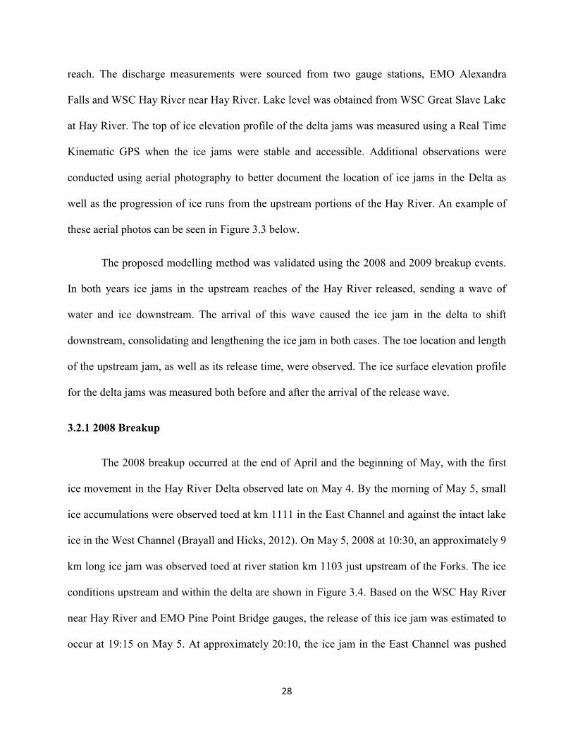
Kinematic GPS when the ice jams were stable and accessible. Additional observations were

conducted using aerial photography to better document the location of ice jams in the Delta as

well as the progression of ice runs from the upstream portions of the Hay River. An example of

these aerial photos can be seen in Figure 3.3 below.

The proposed modelling method was validated using the 2008 and 2009 breakup events.

In both years ice jams in the upstream reaches of the Hay River released, sending a wave of

water and ice downstream. The arrival of this wave caused the ice jam in the delta to shift

downstream, consolidating and lengthening the ice jam in both cases. The toe location and length

of the upstream jam, as well as its release time, were observed. The ice surface elevation profile

for the delta jams was measured both before and after the arrival of the release wave.

3.2.1 2008 Breakup

The 2008 breakup occurred at the end of April and the beginning of May, with the first

ice movement in the Hay River Delta observed late on May 4. By the morning of May 5, small

ice accumulations were observed toed at km 1111 in the East Channel and against the intact lake

ice in the West Channel (Brayall and Hicks, 2012). On May 5, 2008 at 10:30, an approximately 9

km long ice jam was observed toed at river station km 1103 just upstream of the Forks. The ice

conditions upstream and within the delta are shown in Figure 3.4. Based on the WSC Hay River

near Hay River and EMO Pine Point Bridge gauges, the release of this ice jam was estimated to

occur at 19:15 on May 5. At approximately 20:10, the ice jam in the East Channel was pushed

29

downstream by 0.55 km and the jam significantly lengthened and thickened. This ice jam

remained in place over May 6 and resulted in severe flooding. During the time span of this

breakup event, several top of ice surveys were conducted in the delta. The profiles surveyed on

May 5 and May 6 were deemed representative of the conditions before and after the arrival of the

ice jam release wave.

The 9 km ice jam upstream of the delta was observed from reconnaissance flights of the

river (Watson et al. 2009) but its profile was not measured. Therefore, the initial ice jam profile

was calibrated against water levels measured at two gauges at km 1095 (WSC Gauge of Hay

River at Hay River) and km 1098 (EMO Pine Point Bridge Gauge), both located within the

length of the ice jam. Figure 3.5 shows the magnitude of water level increase caused by the ice

jam as calculated from River1D and measured from the two gauge stations. The calibrated ice

jam underside roughness Manning’s n was 0.05. For the release of this ice jam, the empirical

parameters describing the ice resistance and dispersion effects 1 and 2 were calibrated to be 3

and 0, respectively, which best modelled the wave travel time from the release location to the

delta estimated based on field observations. The bank resistance parameter (1) was previously

found to range from 0 to 3.5 for accurate modelling of the propagation of release waves on

various rivers (She and Hicks, 2006). The calibrated value of 3 was considered reasonable as the

distance from the release location to the delta was within two jam lengths, indicating the effects

of bank resistance were significant. The hydrograph at the Forks was output from the River1D

Ice Jam Release model and used as the upstream boundary condition in the River1D Network

model, in which it was then routed downstream in the delta channels. The modelled hydrograph

at the Forks, as well as the hydrographs in the East and West Channel just downstream of the

30

Forks, are depicted in Figure 3.6. Approximately 65% of the flow went into the East Channel

and 35% into the West Channel.

Ice jam profiles in the delta channels were calculated using HEC-RAS. Carrier discharge

before the ice jam release was used for calculating the pre-wave profile while the peak

discharges from the River1D Network model were used for simulating the post-wave profile. In

calibrating with the pre-wave survey, a Manning’s n of 0.06 was used for the underside

roughness of the delta ice jam. The same value was used in modelling the post wave jam. The toe

location was manually moved from km 1111 as for pre-wave jam to km 1111.55 for post wave

jam. Figures 3.7 and 3.8 show the modelled ice jam profiles in the East Channel and the West

Channel respectively, both before and after the wave arrival. The top of ice profile was surveyed

for the East Channel jam both before and after wave arrival, and for the West Channel post wave

jam only. These measurements are also shown in the figures for comparison. The computed

elevation of the top of the ice compares favorably to that of the field measurements in both

channels of the delta, with an average difference of 0.27 m in the East Channel and 0.32 m in the

West Channel.

3.2.2 2009 Breakup

Much like the 2008 event, the 2009 breakup also began in early May, with ice movement

first observed at approximately 02:00 on May 3. Small ice accumulations within the delta were

observed on the same day. After some minor consolidation events, the delta ice jams toed at

around km 1112 in both East and West Channels on May 5. A sequence of three ice jams in the

upper reach of the Hay River was first observed at 14:00 on May 4, one 1.4 km long toed at km

1049, one 1.1 km long toed at km 1047.1, and one 4.3 km long toed at km 1045. They later

31

released at 2:00 on May 6, sending a release wave downstream to the small ice jams in the delta.

The ice conditions both upstream and within the delta are shown in Figure 3.9. Ice movement in

the delta was observed at around 5:00 on May 6. By May 7, the ice jam had shifted even further

downstream the East Channel, nearly reaching the mouth of Great Slave Lake. During this event,

surveyors measured eight top of ice jam profiles throughout the progression of breakup in both

the East Channel and the Fishing Village and Rudd Channels of the West Channel. The surveyed

top of ice profile on May 5 and May 7 were deemed representative of the pre-wave and post-

wave ice jam conditions in the delta. Like the 2008 breakup, both pre-wave and post wave

profiles were surveyed for the East Channel ice jam but only a post wave profile was surveyed

for the West Channel ice jam.

The release of the three ice jams upstream had been modelled in a previous study with the

River1D Ice Jam Release model (Watson et al., 2009) and the same parameters were used here.

Underside roughness of the released jams was set to 0.06, and both 1 and 2 were set to 0. The

toe of the furthest downstream ice jam was over 50 km upstream of the Hay River Delta, so

effects of ice resistance would no longer affect the wave by the time it reached the delta. Again,

the hydrograph at the Forks was output from the River1D Ice Jam Release model. It is shown in

Figure 3.10 along with the hydrographs in the East and West channels as calculated by the

River1D Network model. Approximately 65% of the flow went into the East Channel and 35%

into the West Channel.

Ice jam profiles in the delta channels were calculated using HEC-RAS. Carrier discharge

before the ice jam release was used for calculating the pre-wave profile while the peak

discharges from the River1D Network model were used for simulating the post-wave profile.

Calibrated against the pre-wave ice jam surface profile, a Manning’s n of 0.05 was used for the

32

underside roughness of the delta ice jam. The same values were used for the post-wave jam with

the jam toe shifted from km 1112.36 to km 1113.22. The modelled ice jam profiles together with

the surveyed top of ice profiles in the East Channel and West Channel are shown in Figure 3.11

and Figure 3.12. The post-wave profiles in the Delta compared favorably with those measured

for this event, with an average distance of 0.19 m in the East Channel and 0.14 m in the West

Channel, apart from some higher observation values linked to the inability of the 1-D model to

capture the 2-D transverse variations in the top of ice elevations.

33

Figure 3.1 Locations of ADCP cross sections in the Hay River Delta (Brayall 2011).

34

Figure 3.2 Comparison of flow apportionment into East Channel between River1D Network

model and River2D (Brayall and Hicks, 2012).

0

100

200

300

400

500

600

700

0 200 400 600 800 1000 1200

Flo

w I

n E

ast

Ch

an

nel

(m

3/s

)

Flow into Hay River Delta (m3/s)

River2D

River1D Network model

35

Figure 3.3 Example aerial photo of ice jam in the East Channel of the Hay River Delta taken

May 5, 2008 (Brayall 2011).

36

Figure 3.4 Calibration of 2008 upstream ice jam using data from WSC Hay River near Hay River

and EMO gauge at Pine Point Bridge.

Figure 3.5 Ice Jam Map for modelled 2008 release (adapted from Hicks et al., 1992).

0

0.5

1

1.5

2

2.5

3

3.5

4

4.5

1080 1085 1090 1095 1100 1105 1110

Wa

ter L

evel

Ch

an

ge

Du

e to

Ice

Ja

m

Fo

rma

tio

n (

m)

River Station (km)

PPB Gauge

WSC HR Gauge

River1D

130

150

170

190

210

230

250

270

290

945 955 965 975 985 995 1005 1015 1025 1035 1045 1055 1065 1075 1085 1095 1105

Ele

va

tio

n (

m)

River Distance (km)

Bed Elevation

2008 Ice Jam Location

Ale

xan

dra

Fal

ls

Lo

uis

e F

alls

WS

C G

auge

The

Fo

rks

EM

O-P

PB

Gau

ge

NW

T/A

B B

ord

er

WS

C G

reat

Slv

ae L

ake

Gau

ge

37

Figure 3.6 Ice jam release hydrograph for the 2008 release event modelled with the River1D

Network model.

0

200

400

600

800

1000

-1 1 3 5 7 9 11 13 15

Dis

cha

rge

(m3/s

)

Time from Release (hrs)

Delta Inflow East Channel West Channel

38

Figure 3.7 Pre a) and post b) wave delta ice jam configurations for East Channel-2008.

150

152

154

156

158

160

162

164

166

1106 1107 1108 1109 1110 1111 1112 1113 1114

Ele

va

tio

n (

m)

River Distance (km)

Surveyed Top of Ice

Modelled Ice Jam

Thalweg

a)

150

152

154

156

158

160

162

164

166

1106 1107 1108 1109 1110 1111 1112 1113 1114

Ele

va

tio

n (

m)

River Distance (km)

Surveyed Top of Ice

Modelled Ice Jam

Thalweg

b)

39

Figure 3.8 Pre a) and post b) wave delta ice jam configurations for West Channel-2008.

152

154

156

158

160

162

164

166

1106 1107 1108 1109 1110 1111 1112 1113 1114

Ele

va

tio

n (

m)

River Distance (km)

Modelled Ice Jam

Thalweg

a)

152

154

156

158

160

162

164

166

1106 1107 1108 1109 1110 1111 1112 1113 1114

Ele

va

tio

n (

m)

River Distance (km)

Surveyed Top of Ice

Modelled Ice Jam

Thalweg

b)

40

Figure 3.9 Ice Jam Map for modelled 2009 release (adapted from Hicks et al., 1992).

Figure 3.10 Ice jam release hydrograph for the 2009 release event modelled with the River1D

Network model.

130

150

170

190

210

230

250

270

290

945 955 965 975 985 995 1005 1015 1025 1035 1045 1055 1065 1075 1085 1095 1105

Ele

va

tio

n (

m)

River Distance (km)

Bed Elevation

2009 Ice Jam Location

Ale

xan

dra

Fal

ls

Lo

uis

e F

alls

WS

C G

auge

The

Fo

rks

EM

O-P

PB

Gau

ge

NW

T/A

B B

ord

er

WS

C G

reat

Slv

ae L

ake

Gau

ge

0

100

200

300

400

500

600

700

800

900

1000

0 2 4 6 8 10 12 14

Dis

cha

rge

(m3/s

)

Time from Release (hrs)

Inlet Inflow East Channel West Channel

41

Figure 3.11 Pre (a) and post b) wave delta ice jam configurations for East Channel-2009.

150

152

154

156

158

160

162

164

166

1106 1107 1108 1109 1110 1111 1112 1113 1114

Ele

va

tio

n (

m)

River Distance (km)

Surveyed Top of Ice

Modelled Ice Jam

Thalweg

a)

150

152

154

156

158

160

162

164

166

1106 1107 1108 1109 1110 1111 1112 1113 1114

Ele

va

tio

n (

m)

River Distance (km)

Surveyed Top of Ice

Modelled Ice Jam

Thalweg

b)

42

Figure 3.12 Pre (a) and post b) wave delta ice jam configurations for West Channel-2009.

152

154

156

158

160

162

164

166

1106 1107 1108 1109 1110 1111 1112 1113 1114

Ele

va

tio

n (

m)

River Distance (km)

Modelled Ice Jam

Thalweg

a)

152

154

156

158

160

162

164

166

1106 1107 1108 1109 1110 1111 1112 1113 1114

Ele

va

tio

n (

m)

River Distance (km)

Surveyed Top of Ice

Modelled Ice Jam

Thalweg

b)

43

Chapter 4 : Model Application

4.1 Hypothetical Scenarios

The validated new modelling methodology was then used to simulate a series of

hypothetical events. The top of ice profiles obtained from these events would provide a data set

that was then statistically analysed to develop relationships between the variables defining them

and the resulting profiles. These relationships would form the basis of a flood level prediction

tool in the delta. The East Channel was focussed on due to the large amount of data available for

this channel; however, the same method could easily be applied to the West Channel. Each

hypothetical event modelled consisted of a unique combination of upstream ice jam

configuration and delta jam configuration. Five key variables were identified: the length and toe

location of the upstream ice jam, the carrier discharge at release, the distance of the toe shift of

the delta ice jam in the East Channel, and the water level at the Great Slave Lake. These

variables have direct effect on either the peak flow in the delta caused by upstream ice jam

release or the potential severity of the post wave jam. Additionally, with the exception of the

delta jam toe shift, each of these variables can be measured in the field well in advance of any

flooding events that may occur in the delta, making them ideal for use in a flood prediction tool.

Multiple configurations of the pre-wave delta ice jam were also tested, with the jam length

ranging from 3-5 km, the toe location ranging from km 1110-1112, and the lake level ranging

from 156.6 m to 158.6 m. These tests showed that for the same incoming wave hydrograph, the

percentage of discharge entering the East Channel of the delta was only affected by the different

pre-wave jam condition for approximately 0.5 to 3.0%. This indicated that the pre-wave jam

configuration has minimal effect on the flow apportionment between the East and West

Channels. As the peak discharge in each individual channel decides the post wave jam

44

configuration, a single pre-wave jam across all hypothetical events was deemed adequate. The

underside roughness of both the upstream ice jam and the delta jam used a Manning’s n of 0.06.

1 and 2 were set based on the 2008 and 2009 model validation runs, i.e. 1 = 3 and 2 = 0 if the

distance between the release location and the delta was within 2 jam lengths and 1 = 0 and 2 =

0 otherwise.

Historical records were reviewed for selecting a range of values of each key variable. The

largest discharge recorded on the Hay River during breakup was 1240 m3/s, occurred on May 2,

1974, in the WSC gauge records. The range of simulated carrier discharges was 200 m3/s to 1200

m3/s with 200 m

3/s increments. Documented historical ice jams in the upper reaches of the Hay

River were reviewed, with the relevant information listed in Table 4.1 (Gerard and Stanley,

1988, Kovachis 2011). It was noticed that ice jams in these records with a length exceeding 10

km all melted in place. Therefore, the longest simulated upstream ice jam was 10 km. Four jam

lengths, 2.5 km, 5 km, 7.5 km, and 10 km were simulated in the hypothetical events. Typical toe

locations of the upstream ice jam were also reviewed. The most downstream location considered

was km 1100, as jams have been rarely observed between this location and the entrance of the

delta. To determine the upper limit of the toe location, a few simulation runs were conducted and

it was shown that ice jams toed upstream of Alexandra Falls all produced lower or similar peak

flows at the delta. Because of this, the most upstream toe location considered was km 1020. The

modelled toe locations were placed at 10 km intervals except for the region containing Alexandra

Falls and Louise Falls, as realistic ice jam profiles could not be generated in the model due to the

steep slope and high flow velocities.

45

Table 4.1 List of documented historical ice jam events in the upstream reaches of the Hay River.

Year Date Toe Location (km) Length (km) Carrier Discharge

(m3/s)

Notes

1963 April 30 1073

1988 April 24 1055.42 14 135 Deteriorated

1988 April 26 1059.92 16 221 Deteriorated

1992 April 26 1090

309

1992 April 28 1105

900

2005 April 22 1048

259

2005 April 23 1071

451

2005 April 23 1088.5

451

2007 April 25 1025.9 4.8 290

2007 April 26 958.2 6.7 450

2007 April 26 949.5 9.5 450

2007 April 26 1103 28 450 Deteriorated

2008 May 4 992.5 6.2 450

2008 May 4 1051 6 650

2008 May 5 1103 9 500 Released

2009 May 5 948.6 2.6 550

2009 May 6 1049 1.4 550 Released

2009 May 6 1047.1 1.1 550 Released

2009 May 6 1045 4.3 550 Released

2010 April 23 986

140

2010 April 23 1040.5

140

2011 May-05 1048 5 238

2011 May-06 1068 5 365

2011 May-08 1101 22 478 Deteriorated

Delta ice jam configuration was also selected based on historical observations,

summarized in Table 4.2 (Gerard and Stanley, 1988, Kovachis 2011). The pre-wave jam in the

delta was configured as 4.5 km long with a toe location of km 1111 in the East Channel, based

on the most typical toe location in years where flooding did not occur, as well as the known toe

location of the delta ice jams in 2008 and 2009 before consolidation occurred (Gerard and

Stanley, 1988). Significant flooding has been associated with the shifting of ice jam toes past km

1111 in the East Channel (Gerard and Stanley, 1988). Therefore, a range of potential toe shifts

46

was selected moving downstream from km 1111 encompassing small to big shift distance. These

toe shifts were simulated by changing the toe location of the post-wave ice jam, while keeping

the same head location upstream of the delta. The modelled values of lake level ranged between

156.6 m and 158.6 m based on lake levels observed that corresponded to documented historical

jam events (Brayall and Hicks, 2012). The values simulated for the five key variables are listed

in Table 4.3. Each possible combination of the five key variables was simulated using the 1-D

integrated modelling method described in Chapter 3. The top of ice levels were output for each

scenario at an approximately 0.5 km intervals between km 1108 and km 1114.24 in the East

Channel. In total 1612 unique profiles were obtained from the variables.

47

Table 4.2 List of documented historical ice jams in the Hay River Delta.

Year Date Toe (km) Head (km) Discharge

(m3/s)

Flooding

1950 May 07 1111

Some

1954 May 16 1111.5

1150 None

1956 May 06 1111 1108.9

Some

1957 May 03 1112.4

Some

1963 May 01 ~1112

Significant

1965 May 02 1111.15

750 Some

1974 May 01 1112.25

1100 Significant

1977 May 02 1110

500 None

1978 May 04 1111.5

793 Significant

1979 May 14 1111.5

580 Some

1985 May 05 1112.25 1107.6 1000 Significant

1986 May 04 1111.7 US Delta* 487 Significant

1987 April 29 1111 1106 965 None

1988 April 27 1110.9 1098.4 605 None

1988 April 30 1111 1104.6 353 None

1989 May 03 1112 1082 1140 Significant

1989 May 06 1111.5 US Delta 900 Significant

1990 April 28 1111 US Delta 560 None

1991

1111 US Delta 460 None

1992 April 26 1111.5

309 Significant

1992 April 28 1112.6 1105 900 Significant

2005 April 25 1111.3 1108 491 Some

2008 May 05 1110.8 US Delta 500 Significant

2008 May 06 1111.5 US Delta 893 Significant

2009 May 03 1110.8 US Delta 268 Some

2009 May 04 1111.2 US Delta 500 Some

2009 May 05 1111.8 US Delta 670 Some

2009 May 07 1111.8 US Delta 900 Some

*“US Delta” indicates an ice jam extending upstream of the delta by an unknown distance

48

Table 4.3 Selected values of key variables in the simulated hypothetical events.

Release Jam Length

(km)

Release Jam Toe

Location (km)

Carrier Toe Shift

(km)

Downstream Lake

Level (m) Discharge

(m3/s)

1 2.5 1020 200 0.55 156.6

2 5 1030 400 1.2 157.1

3 7.5 1050 600 1.4 157.6

4 10 1060 800 2.22 158.6

5 - 1070 1000 - -

6 - 1080 1200 - -

7 - 1090 - - -

8 - 1100 - - -

4.2 Multiple Linear Regression (MLR) Analyses

Multiple linear regression analyses were employed to develop relationships between the

simulated top of ice levels (TOI) in the delta region and the five selected variables, the length

(Lj) and toe location (Tj) of the upstream ice jam, carrier discharge (Qc), toe shift of the delta

jam (TS), and the lake level (LL). The MLR analyses were applied to develop a series of

regression equations at ten locations in the East Channel of the delta. These locations are the

same as where the top of ice levels were output for the simulated hypothetical events. The

general format of the regression equations is shown below.

𝑇𝑂𝐼 = 𝑎1𝐿𝑗 + 𝑎2𝑇𝑗 + 𝑎3𝑄𝑐 + 𝑎4𝑇𝑆 + 𝑎5𝐿𝐿 + 𝑎6 (4-1)

where aj (j = 1, 6) are the regression coefficients.

Multiple equations divided around values of a single variable were found to produce

better results at each location when compared to a single equation. The top of ice levels in the

delta region upstream of km 1111.55 were found to be most sensitive to the carrier discharge of

49

the river. Therefore three regression equations were developed for each of the 5 locations in this

region: one for low carrier discharges (QC ≤ 500 m3/s), one for medium carrier discharges (QC =

501 – 900 m3/s), and one for high carrier discharges (QC > 900 m

3/s). In the toe region of the

jam, between km 1111.55 and 1113.22, the top of ice levels had a distinct relationship with each

toe shift, thus each had an individual regression equation. At km 1113.22, the top of ice levels

were sensitive to a combination of carrier discharge, downstream lake level, and toe shift. Four

regression equations were developed here, two for the first three toe shifts corresponding to LL <

157.6 m and LL ≥ 157.6 m, and two for the largest toe shift (TS = 2.22 km) corresponding to Qc

≤ 600 m3/s and Qc > 600 m

3/s respectively. At km 1113.6 the top of ice levels were most

sensitive to the lake level, requiring only two equations, one for LL < 157.6 m and one for LL ≥

157.6 m. The coefficients of the equations are summarized in Table 4.4.

Each regression equation is also associated with an average error value between the

modelled top of ice elevation from the hypothetical events and the elevation predicted by the

equation, a coefficient of determination indicating the closeness of fit of the equation, and a set

of p-values for each variable indicating the strength of the relationship between the individual

variables and the response. All the regression equations had low average errors (0.0396 m -0.431

m), relatively high values of the coefficient of determination (80-95%), and extremely low p-

values (0.0001-0.0003) indicating a strong relationship between the top of ice level and the

selected variables. The values of the average error for each regression equation are also listed in

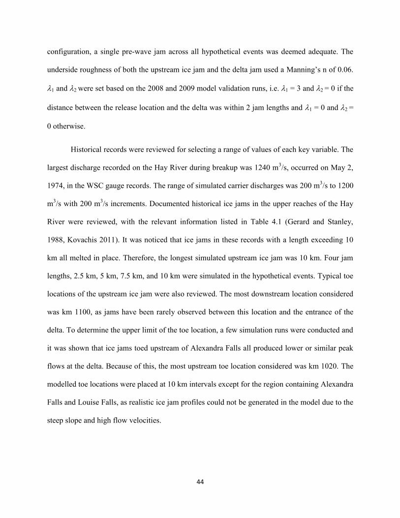
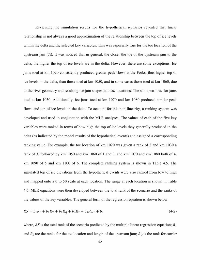
Table 4.4. The results of the equations at each location are shown in Figures 4.1-4.10a, presented

in terms of the simulated top of ice levels versus the top of ice levels predicted by the regression

equations. It can be seen that although the regression equations produced reasonable predictions

of top of ice levels, there are certain levels of scatter in the figures.

50

Table 4.4 List of MLR equations for each location in the East Channel of the Hay River Delta.

Location (km) Equation Criteria a1 a2 a3 a4 a5 a6 Regression Error (m)

1108.3

QC ≤ 500 m3/s 0.114 0.00885 0.00685 0.0415 0.128 129.56 0.291

QC = 501 – 900 m3/s 0.173 0.0138 0.00422 0.0284 0.14 123.33 0.359

QC > 900 m3/s 0.205 0.0228 0.00357 0.0685 0.164 110.29 0.322

1109.04

QC ≤ 500 m3/s 0.104 0.00784 0.0062 0.0462 0.121 131.45 0.265

QC = 501 – 900 m3/s 0.161 0.0129 0.00388 0.0397 0.139 123.98 0.342

QC > 900 m3/s 0.188 0.0172 0.00342 0.0768 0.146 118.65 0.363

1109.5

QC ≤ 500 m3/s 0.0998 0.00723 0.00588 0.0472 0.128 130.82 0.255

QC = 501 – 900 m3/s 0.154 0.0122 0.00368 0.0421 0.145 123.57 0.331

QC > 900 m3/s 0.183 0.0165 0.0033 0.0752 0.151 118.27 0.352

1109.98

QC ≤ 500 m3/s 0.0988 0.00681 0.00571 0.0161 0.163 125.37 0.252

QC = 501 – 900 m3/s 0.147 0.0113 0.00344 0.0009 0.163 121.44 0.318

QC > 900 m3/s 0.175 0.0155 0.00314 0.0138 0.158 117.85 0.337

1111.01

QC ≤ 500 m3/s 0.0972 0.00626 0.00542 -0.0543 0.143 128.34 0.252

QC = 501 – 900 m3/s 0.14 0.0104 0.00318 -0.106 0.165 121.6 0.313

QC > 900 m3/s 0.168 0.0144 0.00295 -0.0727 0.176 115.5 0.322

51

Table 4.4 List of MLR equations for each location in the East Channel of the Hay River Delta (continued).

Location (km) Equation Criteria a1 a2 a3 a4 a5 a6 Regression Error (m)

1111.55

TS = 0.55 km 0.114 0.00597 0.00309 n/a 0.163 124.86 0.462

TS = 1.2 km 0.137 0.0104 0.00396 n/a 0.0726 134.75 0.356

TS = 1.4 km 0.132 0.0104 0.00381 n/a 0.0862 132.71 0.334

TS = 2.2 km 0.138 0.0111 0.00393 n/a 0.135 124.1 0.352

1112.2

TS = 0.55 km 0.0422 0.00043 0.00111 n/a 0.671 50.9 0.223

TS = 1.2 km 0.102 0.00651 0.00241 n/a 0.51 69.33 0.354

TS = 1.4 km 0.132 0.0103 0.00368 n/a 0.0668 135.21 0.339

TS = 2.2 km 0.142 0.0118 0.00416 n/a 0.1 128.12 0.372

1112.36

TS = 0.55 km 0.04 0.00046 0.00106 n/a 0.684 48.76 0.209

TS = 1.2 km 0.0545 0.00473 0.00163 n/a 0.817 23.34 0.262

TS = 1.4 km 0.115 0.00704 0.00301 n/a 0.541 63.94 0.382

TS = 2.2 km 0.142 0.0119 0.00417 n/a 0.0973 128.39 0.376

1113.22

LL < 157.6 m & TS < 2.2 km 0.0228 0.00114 0.0009 0.00052 0.695 46.38 0.0921

LL ≥ 157.6 m & TS < 2.2 km 0.0358 0.00371 0.00088 0.158 0.689 44.42 0.167

Qc ≤ 600 m3/s & TS = 2.22 km 0.0599 0.00377 0.002 n/a 0.976 -1.14 0.264

Qc > 600 m3/s & TS = 2.22 km 0.115 0.0114 0.00239 n/a 0.538 59.24 0.313

1113.6 LL < 157.6 m 0.0125 0.00067 0.00048 0.00014 0.832 25.45 0.0522

LL ≥ 157.6 m 0.021 0.00182 0.00044 0.034 0.831 24.36 0.0868

52

Reviewing the simulation results for the hypothetical scenarios revealed that linear

relationship is not always a good approximation of the relationship between the top of ice levels

within the delta and the selected key variables. This was especially true for the toe location of the

upstream jam (Ti). It was noticed that in general, the closer the toe of the upstream jam to the

delta, the higher the top of ice levels are in the delta. However, there are some exceptions. Ice

jams toed at km 1020 consistently produced greater peak flows at the Forks, thus higher top of

ice levels in the delta, than those toed at km 1050, and in some cases those toed at km 1060, due

to the river geometry and resulting ice jam shapes at these locations. The same was true for jams

toed at km 1030. Additionally, ice jams toed at km 1070 and km 1080 produced similar peak

flows and top of ice levels in the delta. To account for this non-linearity, a ranking system was

developed and used in conjunction with the MLR analyses. The values of each of the five key

variables were ranked in terms of how high the top of ice levels they generally produced in the

delta (as indicated by the model results of the hypothetical events) and assigned a corresponding

ranking value. For example, the toe location of km 1020 was given a rank of 2 and km 1030 a

rank of 3, followed by km 1050 and km 1060 of 1 and 3, and km 1070 and km 1080 both of 4,

km 1090 of 5 and km 1100 of 6. The complete ranking system is shown in Table 4.5. The

simulated top of ice elevations from the hypothetical events were also ranked from low to high

and mapped onto a 0 to 50 scale at each location. The range at each location is shown in Table

4.6. MLR equations were then developed between the total rank of the scenario and the ranks of

the values of the key variables. The general form of the regression equation is shown below.

𝑅𝑆 = 𝑏1𝑅𝐿 + 𝑏2𝑅𝑇 + 𝑏3𝑅𝑄 + 𝑏4𝑅𝑆 + 𝑏5𝑅𝑊𝐿 + 𝑏6 (4-2)

where, RS is the total rank of the scenario predicted by the multiple linear regression equation; RT

and RL are the ranks for the toe location and length of the upstream jam; RQ is the rank for carrier

53

discharge; RS is the rank for toe shift of the delta jam; RWL is the rank for the lake level; bj (j = 1,

6) are coefficients determined by multiple linear regression analysis. These new equations are

summarized in Table 4.7, with the results of the equations shown in Figures 4.1-4.10b. The

average error of the individual equations was reduced by 0.058 m on average, while the R2 value

at each location increased by 0.0162 on average.

Table 4.5 Rankings of the five key variables.

Release Jam

Length

(Lj)

Release Jam

Toe Location

(Tj)

Carrier

Discharge

(Qc)

Toe Shift

(TS)

Downstream

Lake level

(LL)

(km) Rank (km) Rank (m3/s) Rank (km) Rank (m) Rank

1 2.5 1 1020 2 200 1 0.55 1 156.6 1

2 5 2 1030 3 400 2 1.2 2 157.1 1.5

3 7.5 3 1050 1 600 3 1.4 3 157.6 2

4 10 4 1060 3 800 4 2.22 4 158.6 3

5 - - 1070 4 1000 5 - - - -

6 - - 1080 4 1200 6 - - - -

7 - - 1090 5 - - - - - -

8 - - 1100 6 - - - - - -

54

Table 4.6 Range of modelled top of ice elevations at key locations in the East Channel of the Hay River Delta.

Location (km) 1108.3 1109 1109.5 1109.98 1111 1111.55 1112.2 1112.36 1113.22 1113.61

Minimum Top

of Ice (m) 160.2 159.9 159.5 158.9 158.1 156.9 156.6 156.6 156.63 156.6

Maximum

Top of Ice (m) 168.3 167.3 166.7 165.9 164.9 164.3 164.0 163.9 161.46 159.2

55

Table 4.7 List of rankd MLR equations in the East Channel of the Hay River Delta.

Location (km) Equation Criteria b1 b2 b3 b4 b5 b6 Regression Error (m)

1108.3

SQ ≤ 500 m3/s 1.66 1.24 8.46 0.257 0.788 -12.4 0.235

SQ = 501 – 900 m3/s 2.51 1.94 5.2 0.175 0.866 -8.38 0.238

SQ > 900 m3/s 2.92 2.43 4.42 0.419 0.962 -8.12 0.251

1109

SQ ≤ 500 m3/s 1.63 1.2 8.29 0.309 0.81 -12.1 0.215

SQ = 501 – 900 m3/s 2.52 1.96 5.19 0.265 0.935 -9.04 0.232

SQ > 900 m3/s 2.96 2.47 4.57 0.514 0.974 -9.46 0.236

1109.5

SQ ≤ 500 m3/s 1.65 1.18 8.25 0.331 0.896 -12.2 0.205

SQ = 501 – 900 m3/s 2.54 1.95 5.16 0.295 1.02 -9.25 0.227

SQ > 900 m3/s 3.01 2.48 4.62 0.527 1.06 -10.1 0.231

1109.98

SQ ≤ 500 m3/s 1.67 1.15 8.15 0.115 1.16 -11.6 0.203

SQ = 501 – 900 m3/s 2.47 1.86 4.91 0.0064 1.16 -7.47 0.22

SQ > 900 m3/s 2.94 2.39 4.48 0.0985 1.13 -8.3 0.222

1111

SQ ≤ 500 m3/s 1.67 1.11 7.87 -0.394 1.04 -9.44 0.204

SQ = 501 – 900 m3/s 2.38 1.77 4.6 -0.764 1.19 -4.43 0.222

SQ > 900 m3/s 2.86 2.26 4.27 -0.527 1.28 -6.24 0.215

56

Table 4.7 List of rankd MLR equations in the East Channel of the Hay River Delta (continued).

Location (km) Equation Criteria b1 b2 b3 b4 b5 b6 Regression Error (m)

1111.55

SS = 0.55 km 1.84 1.09 4.15 n/a 1.09 -5.79 0.426

SS = 1.2 km 2.16 1.61 5.32 n/a 0.487 -3.38 0.289

SS = 1.4 km 2.08 1.56 5.12 n/a 0.579 -3.46 0.272

SS = 2.2 km 2.18 1.67 5.28 n/a 0.905 -5.57 0.285

1112.2

SS = 0.55 km 0.674 0.369 1.504 n/a 4.52 -6.32 0.208

SS = 1.2 km 1.63 1.05 3.24 n/a 3.43 -10 0.322

SS = 1.4 km 2.1 1.53 4.95 n/a 0.45 -5.52 0.282

SS = 2.2 km 2.25 1.78 5.59 n/a 0.673 -7.74 0.303

1112.36

SS = 0.55 km 0.653 0.358 1.45 n/a 4.7 -7.07 0.195

SS = 1.2 km 0.877 0.725 2.24 n/a 5.61 -10.9 0.245

SS = 1.4 km 1.87 1.24 4.14 n/a 3.72 -11.6 0.334

SS = 2.2 km 2.3 1.82 5.72 n/a 0.668 -9.21 0.307

1113.22

SWL < 157.6 m & SS < 2.2 km 0.554 0.402 1.86 0.0054 7.19 -11.2 0.0787

SWL ≥ 157.6 m & SS < 2.2 km 0.871 0.725 1.83 1.64 7.14 -13.1 0.165

SQ ≤ 600 m3/s & SS = 2.22 km 1.48 0.874 4.14 n/a 10.1 -20.1 0.254

SQ > 600 m3/s & SS = 2.22 km 2.82 2.26 4.97 n/a 5.57 -24.2 0.3

1113.61 SWL < 157.6 m 0.573 0.43 1.88 0.0027 16.3 -20.6 0.045

SWL ≥ 157.6 m 0.981 0.692 1.72 0.745 16.3 -20.9 0.085

57

4.3 Flood Level Prediction Tool

The rank based regression equations were used as the basis for the development of a

flood level prediction tool for the East Channel of the delta. This tool uses the toe location and

length of the upstream ice jam, the carrier discharge, and the downstream lake level as defined

inputs. These values can be known well in advance of any delta flooding that may occur. The

carrier discharge and lake level can be obtained from WSC or EMO gauge stations. Information

on the upstream ice jam(s) can be obtained through aerial reconnaissance observations. As it is

not possible to accurately predict the distance that the delta jams toe may shift downstream

during consolidation triggered by the incoming release wave, the tool was configured to calculate

four possible top of ice levels for each considered toe shift at each location in the East Channel.

The maximum and minimum values at each location are then output. The sum of the modelling

error as determined from the validation results and the average error of each regression equation

was used to estimate the error bound at each location. The complete code of the prediction tool is

shown in Appendix A.

The accuracy of the prediction tool was evaluated through comparison to two historical

events (1992 and 2007) involving the consolidation of ice jams in the East Channel of the delta.

The results were also compared to predictions by the IJPG developed by Brayall and Hicks

(2012) using 2-D modelling. The 1992 event consisted of an estimated 5 km long jam releasing

from km 1090 with a carrier discharge of 567 m3/s, causing the consolidation of an ice jam in the

delta with a downstream lake level of 157.04 m. The delta ice jam shifted to km 1112.6, resulting

in significant flooding. Figure 4.11 shows the highest and lowest top of ice profiles calculated by

the prediction tool resulting from different toe shifts. The predicted top of ice levels agree

reasonably well with the surveyed top of ice profile, while also providing a much closer

58

representation of the observed profile than the IJPG results for the same jam. Additionally, the

error bounds of the prediction tool are smaller than those of the IJPG, with the exception of

locations where the IJPG calculated values of zero error, a result of the IJPG extrapolating the

peak discharge of the modelled event, which fell outside the range of discharges the IJPG was

developed with. The IJPG also incorrectly captured the top of ice levels of the downstream end

of the reach as it interpolates the lake level based on ratings curves, rather than allowing the lake

level of an event to be specified.

The 2007 event consisted of the release of a 4.8 km long jam toed at km 1025.9 with a

carrier discharge of 290 m3/s. This release shifted an ice jam in the delta to km 1111.3 with a

lake level of 158.62 m, triggering minor flooding in the downstream end of the delta. As the

2007 event did not have any surveyed top of ice values, comparisons were only made to the

elevations of key landmarks within the delta that would denote flooding if exceeded. Figure 4.12

shows the predicted top of ice levels with error bounds below key landmark elevations through

most of the East Channel excepting a region towards the downstream end. Therefore, the tool

provides a reasonable estimate of flood conditions. The predicted top of ice levels from the IJPG

were below the landmark elevations, excepting the upper error bound at km 1110.5, indicating

the prediction tool provides a closer estimate of the flood conditions as compared to the IJPG.

The error bounds were mostly comparative between the two tools except for km 1111 where the

proposed tool has a much smaller error bound than IJPG.

59

Figure 4.1 Comparison between the predicted and the simulated top of ice level at Km 1108.3 for

the two regression methods: a) without rank and b) with rank.

60

Figure 4.2 Comparison between the predicted and the simulated top of ice level at Km 1109 for

the two regression methods: a) without rank and b) with rank.

61

Figure 4.3 Comparison between the predicted and the simulated top of ice level at Km 1109.5 for

the two regression methods: a) without rank and b) with rank.

62

Figure 4.4 Comparison between the predicted and the simulated top of ice level at Km 1109.98

for the two regression methods: a) without rank and b) with rank.

63

Figure 4.5 Comparison between the predicted and the simulated top of ice level at Km 1111 for

the two regression methods: a) without rank and b) with rank.

64

Figure 4.6 Comparison between the predicted and the simulated top of ice level at Km 1111.55

for the two regression methods: a) without rank and b) with rank.

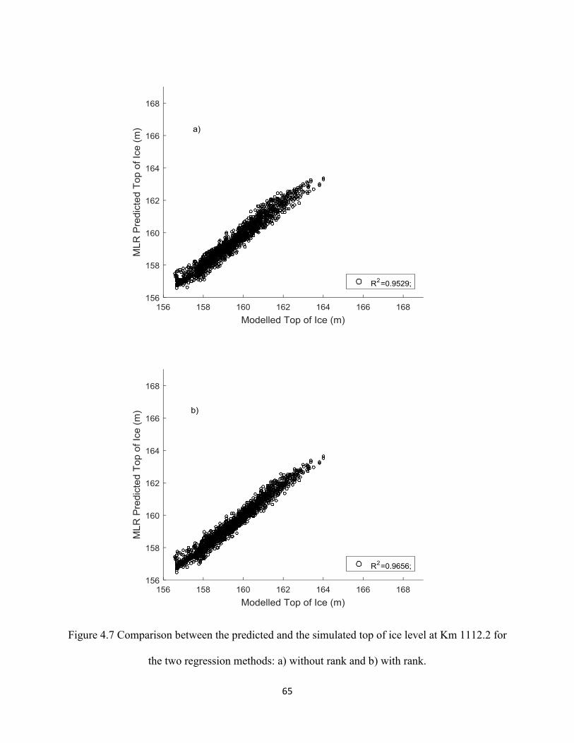
65

Figure 4.7 Comparison between the predicted and the simulated top of ice level at Km 1112.2 for

the two regression methods: a) without rank and b) with rank.

66

Figure 4.8 Comparison between the predicted and the simulated top of ice level at Km 1112.4 for

the two regression methods: a) without rank and b) with rank.

67

Figure 4.9 Comparison between the predicted and the simulated top of ice level at Km 1113.22

for the two regression methods: a) without rank and b) with rank.

68

Figure 4.10 Comparison between the predicted and the simulated top of ice level at Km 1113.61

for the two regression methods: a) without rank and b) with rank.

69

Figure 4.11 Comparison of the top of ice level predicted by the proposed tool, the IJPG and the

observation for the 1992 flooding event.

70

Figure 4.12 Comparison of the top of ice level predicted by the proposed tool, the IJPG and the

key landmarks for the 2007 flooding event.

71

Chapter 5 : Summary and Conclusions

The release of ice jams in the upstream reaches of the Hay River has been identified as an

important factor in the consolidation of ice jams within the Hay River Delta. The consolidation

often leads to much thicker and longer ice jams, resulting in flooding in the delta region and

presenting a threat to the Town of Hay River and other communities situated near or within the

delta. The objective of this research was to develop an operational tool capable of predicting ice

jam flood levels in the delta triggered by ice jam consolidation. This tool utilised a sequence of

three 1-D models, the River1D Ice Jam Release model, the River1D Network model, and the

HEC-RAS model, to simulate the upstream ice jam formation and release, the release wave

propagating through the delta, and the top of ice profile of the consolidated ice jam in the delta.

This new integrated modelling method was validated through comparison to breakup events

occurred in 2008 and 2009 and was shown to produce plausible results when compared to the top

of ice measurements taken during these events, with an average modelling error of 0.242 m.

The validated modelling method was then used to simulate a large quantity of

hypothetical events, covering a variety of potential combinations of upstream and delta ice jam

conditions. Simulated results from these events, specifically the top of ice levels output at key

locations along the East Channel, were then analyzed using MLR analyses. The analyses

produced a series of regression equations describing the relationship between the top of ice level

at different locations along the East Channel and the five variables: carrier discharge, toe

location of the upstream jam, length of the upstream jam, post-wave toe shift of the delta jam,

and the downstream lake level. Two sets of regression equations were developed: one based on

the original values and the other based on ranks of the top of ice levels and the key variables. It

was shown that the regression equations with the ranking system provided a better prediction of

72

the simulated top of ice levels with an average reduction of error of 0.058 m and an average

increase of the R2 value of 0.0162 on average. These equations also demonstrated the sensitivity

of top of ice levels in the delta to the different variables. Upstream locations were sensitive to

carrier discharge, locations in the toe shift region were sensitive to the distance of the toe shift,

and locations in the downstream end of the channel were sensitive to the lake level.

The regression equations obtained with the ranking system were used in the development

of a flood level prediction tool for the Town of Hay River. The tool uses information that can be

available well in advance of any delta flooding as input, producing top of ice profiles for the East

Channel of the delta. A range of possible delta jam toe shifts were considered, allowing the

effects of jam toe shifting during the consolidation event in the delta to be explicitly accounted

for. The accuracy of the tool was compared both to surveyed top of ice levels, documented flood

severity and the results of the previously developed IJPG for two historical events. In both cases,

the results of the proposed prediction tool compared well with the historical events, and provided

improved accuracy and smaller amounts of error in comparison to the results obtained from 2-D

modelling.

The same method as described in this study can be applied to the West Channel for a

complete coverage of flood forecasting for the Hay River Delta. This research also demonstrated

the viability of using 1-D models in simulating ice jam release and subsequent ice jam

consolidation in complex multi-channel networks. Comparable accuracy with 2-D modelling was

achieved yet with much lesser data requirements and modelling efforts. Therefore, further work

is recommended for the development of an integrated 1-D network model which is capable of

predicting ice jam caused flooding in complex multi-channel network systems similar to the Hay

River Delta.

73

References

Blackburn, J., She, Y., Hicks, F., and Nafziger, J., 2015. Ice effects on flow distributions in the

Mackenzie Delta. In Proceedings of 18th Workshop on the Hydraulics of Ice Covered Rivers,

Quebec City, Quebec, 18-20 August, 2015.

Brayall, M., 2011. 2-D hydraulic and ice process modeling at Hay River, NWT. MSc. Thesis,

Department of Civil Engineering, University of Alberta, Edmonton, AB

Brayall, M., and Hicks, F., 2012. Applicability of 2-D modeling for forecasting ice jam flood

levels in the Hay River Delta, Canada. Canadian Journal of Civil Engineering, 39:701-712

Flato, G., and Gerard, R., 1986. Calculation of ice jam thickness profiles. In Proceedings of 4th

Workshop on Hydraulics of River Ice, Subcommittee of Hydraulics of Ice Covered Rivers,

National Research Council of Canada, Montreal, 19-20 June, 1986.

Gerard, R., and Stanley, S., 1988. Ice jams and flood forecasting, Hay River, N.W.T.

Environment Canada and Indian and Northern Affairs Canada, Yellowknife, N.W.T.

Gerard, R., Hicks, F., and Jasek, M., 1990. Ice jams and flood forecasting, Hay River, N.W.T.-

Phase 2: Surges and interactive computer program development. Environment Canada and

Indian and Northern Affairs Canada, Yellowknife, N.W.T.

Hicks, F.E., Steffler, P.M. and Gerard, R., 1992. Finite Element Modeling of Surge Propagation

and an Application to the Hay River, NWT, Canadian Journal of Civil Engineering, 19(3): 454-

462.

74

Kovachis, N. Hicks, F., Zhao, L. and Maxwell, J. 2010. Development of an expert system for

forecasting the progression of breakup at Hay River, NWT, Canada. In Proceedings of 20th

IAHR Ice Symposium, Lahti, Finland, 14-18 June, 2010.

Kovachis, N., 2011. Patterns of river breakup timing and sequencing, Hay River, NWT. MSc.

Thesis, Department of Civil Engineering, University of Alberta, Edmonton, AB

Pariset, E., Hausser, R. and Gagon, A., 1966. Formation of ice covers and ice jams in rivers.

Journal of Hydraulics Division, Proc. of the American Society of Civil Engineers, 92(HY6): 1-

23.

She, Y. and F. Hicks 2005. Incorporating ice effects in ice jam release surge models. In

Proceedings of 13th Workshop on River Ice, Hanover, NH, 16-18 Sept. 2005, CGU-HS CRIPE,

pp. 470-484.

She, Y. and Hicks, F., 2006. Modelling ice jam release waves with consideration for ice effects.

Cold Regions Science and Technology, 45:137-147.

She, Y., Hicks, F., Steffler, P. and Healy, D., 2008. Effects of unsteadiness and ice motion on

river ice jam profiles. In Proceedings of 19th IAHR International Symposium on Ice, Vancouver,

British Columbia, 6-11 July, 2008.

Uzuner, M.S. and J.F. Kennedy 1976. Theoretical model of river ice jams. ASCE Journal of

Hydraulic Engineering, 102(9): 1365-1383.

Watson, D., Hicks, F., and Andrishak, R., 2009. Analysis of observed 2008 ice jam release

events on the Hay River, NWT. In Proceedings of 15th Workshop on River Ice, St John’s,

75

Newfoundland, 15-17 June, 2009. CGU HS Committee on River Ice Processes and the

Environment.

Watson, D., 2011. Observation and modeling of ice jam release events on the Hay River, NWT.

MSc. Thesis, Department of Civil Engineering, University of Alberta, Edmonton, AB

Zhao, L., 2012. River ice breakup forecasting using artificial neural networks and fuzzy logic

systems. MSc thesis, Department of Civil Engineering, University of Alberta, Edmonton, AB.

76

Appendix A: Matlab Code of the Flood Level Prediction Tool

77

clc; clear; importfile('Data Analysis');

%User Defined Scenario Input Length=4.8; Toe=1025.9; Flow=290; Lake=158.62;

%Conversion of Scenario to rank L=Length/2.5;

if Toe<=1030 T=2; elseif Toe>=1050 && Toe<1060 T=(Toe-1050)/5+1; elseif Toe>=1060 && Toe<1070 T=(Toe-1060)/10+3; elseif Toe>=1070 && Toe<1080 T=4; elseif Toe>=1080 T=(Toe-1080)/10+4; end

F=Flow/200; l=Lake-155.6; n=1

for j=1:4 rank(j,1)=L; rank(j,2)=T; rank(j,3)=F; rank(j,4)=j; rank(j,5)=l; end

%Calculation of top of ice values for km 1108.3 for k=1:4 if input(1,3)<= 500 sumrankA(k,1)=-12.4 +1.66*rank(k,1) +1.24*rank(k,2)

+8.46*rank(k,3)+.257*rank(k,4)+.788*rank(k,5); sumrankA(k,4)=.235 elseif input(1,3)>= 901 sumrankA(k,1)=-8.12 +2.92*rank(k,1) +2.43*rank(k,2)

+4.42*rank(k,3)+.419*rank(k,4)+.962*rank(k,5); sumrankA(k,4)=.251 else sumrankA(k,1)=-8.38 +2.51*rank(k,1) +1.94*rank(k,2)

+5.2*rank(k,3)+.175*rank(k,4)+.866*rank(k,5); sumrankA(k,4)=.238 end sumrankA(k,2)=1108.3; sumrankA(k,3)=(sumrankA(k,1)/50)*(168.26-160.16)+160.16; end

78

graphrank(1,1)=max(sumrankA(:,3)); graphrank(1,2)=min(sumrankA(:,3)); graphrank(1,3)=sumrankA(1,4); graphrank(1,4)=sumrankA(1,4);

%Calculation of top of ice values for km 1109 for k=1:4 if input(1,3)<= 500 sumrankB(k,1)=-12.1+1.63*rank(k,1)+1.2*rank(k,2)+8.29*rank(k,3)

+.309*rank(k,4)+.81*rank(k,5); sumrankB(k,4)=.215 elseif input(1,3)>= 901 sumrankB(k,1)=-9.46+2.96*rank(k,1)+2.47*rank(k,2)+4.57*rank(k,3)

+.514*rank(k,4)+.974*rank(k,5); sumrankB(k,4)=.236 else sumrankB(k,1)=-9.04+2.52*rank(k,1)+1.96*rank(k,2)+5.19*rank(k,3)

+.265*rank(k,4)+.935*rank(k,5); sumrankB(k,4)=.232 end sumrankB(k,2)=1109; sumrankB(k,3)=(sumrankB(k,1)/50)*(167.333-159.85)+159.85; end

graphrank(2,1)=max(sumrankB(:,3)); graphrank(2,2)=min(sumrankB(:,3)); graphrank(2,3)=sumrankB(1,4); graphrank(2,4)=sumrankB(1,4);

%Calculation of top of ice values for km 1109.5 for k=1:4 if input(n,3)<= 500 sumrankC(k,1)=-12.2+1.65*rank(k,1)+1.18*rank(k,2)+8.25*rank(k,3)

+.331*rank(k,4)+.896*rank(k,5); sumrankC(k,4)=.205 elseif input(n,3)>= 901 sumrankC(k,1)=-10.1+3.01*rank(k,1)+2.48*rank(k,2)+4.62*rank(k,3)

+.527*rank(k,4)+1.06*rank(k,5); sumrankC(k,4)=.231 else sumrankC(k,1)=-9.25+2.54*rank(k,1)+1.95*rank(k,2)+5.16*rank(k,3)

+.295*rank(k,4)+1.02*rank(k,5); sumrankC(k,4)=.227 end sumrankC(k,2)=1109.5; sumrankC(k,3)=(sumrankC(k,1)/50)*(166.67-159.54)+159.54; end

graphrank(3,1)=max(sumrankC(:,3)); graphrank(3,2)=min(sumrankC(:,3)); graphrank(3,3)=sumrankC(1,4); graphrank(3,4)=sumrankC(1,4);

79

%Calculation of top of ice values for km 1109.98 for k=1:4 if input(n,3)<= 500 sumrankD(k,1)=-11.6+1.67*rank(k,1)+1.15*rank(k,2)+8.15*rank(k,3)

+.115*rank(k,4)+1.16*rank(k,5); sumrankD(k,4)=.203 elseif input(n,3)>= 901 sumrankD(k,1)=-8.3+2.94*rank(k,1)+2.39*rank(k,2)+4.48*rank(k,3)

+.0985*rank(k,4)+1.13*rank(k,5); sumrankD(k,4)=.222 else sumrankD(k,1)=-7.47+2.47*rank(k,1)+1.86*rank(k,2)+4.91*rank(k,3)

+.0064*rank(k,4)+1.16*rank(k,5); sumrankD(k,4)=.22 end sumrankD(k,2)=1109.98; sumrankD(k,3)=(sumrankD(k,1)/50)*(165.98-158.98)+158.98; end

graphrank(4,1)=max(sumrankD(:,3)); graphrank(4,2)=min(sumrankD(:,3)); graphrank(4,3)=sumrankD(1,4); graphrank(4,4)=sumrankD(1,4);

%Calculation of top of ice values for km 111 for k=1:4 if input(n,3)<= 500 sumrankE(k,1)=-9.44+1.67*rank(k,1) +1.11*rank(k,2) +7.87*rank(k,3)-

.394*rank(k,4) +1.04*rank(k,5); sumrankE(k,4)=.204 elseif input(n,3)>= 901 sumrankE(k,1)=-6.24+2.86*rank(k,1)+2.26*rank(k,2) +4.27*rank(k,3)-

.527*rank(k,4)+1.28*rank(k,5); sumrankE(k,4)=.215 else sumrankE(k,1)=-4.43+2.38*rank(k,1)+1.77*rank(k,2) +4.6*rank(k,3)-

.764*rank(k,4)+1.19*rank(k,5); sumrankE(k,4)=.222 end sumrankE(k,2)=1111; sumrankE(k,3)=(sumrankE(k,1)/50)*(164.98-158.08)+158.08; end

graphrank(5,1)=max(sumrankE(:,3)); graphrank(5,2)=min(sumrankE(:,3)); graphrank(5,3)=sumrankE(1,4); graphrank(5,4)=sumrankE(1,4);

80

%Calculation of top of ice values for km 1111.55 for k=1:4 if rank(k,4)== 1 sumrankF(k,1)=-5.79+1.84*rank(k,1)+1.09*rank(k,2)

+4.15*rank(k,3)+1.09*rank(k,5); sumrankF(k,4)=.426 elseif rank(k,4)== 2 sumrankF(k,1)=-3.38+2.16*rank(k,1)+1.61*rank(k,2)

+5.32*rank(k,3)+.487*rank(k,5); sumrankF(k,4)=.289 elseif rank(k,4)==3 sumrankF(k,1)=-3.46+2.08*rank(k,1)+1.56*rank(k,2)

+5.12*rank(k,3)+.579*rank(k,5); sumrankF(k,4)=.272 else sumrankF(k,1)=-5.57+2.18*rank(k,1)+1.67*rank(k,2)

+5.28*rank(k,3)+.905*rank(k,5); sumrankF(k,4)=.285 end sumrankF(k,2)=1111.55; sumrankF(k,3)=(sumrankF(k,1)/50)*(164.32-156.87)+156.87; end

graphrank(6,1)=max(sumrankF(:,3)); graphrank(6,2)=min(sumrankF(:,3));

for k=1:4 if graphrank(6,1)==sumrankF(k,3) graphrank(6,3)=sumrankF(k,4); end

if graphrank(6,2)==sumrankF(k,3) graphrank(6,4)=sumrankF(k,4); end end

81

%Calculation of top of ice values for km 1112.2 for k=1:4 if rank(k,4)== 1 sumrankG(k,1)=-6.32+.674*rank(k,1)+.369*rank(k,2)

+1.504*rank(k,3)+4.52*rank(k,5); sumrankG(k,4)=.208 elseif rank(k,4)== 2 sumrankG(k,1)=-10+1.63*rank(k,1)+1.05*rank(k,2)

+3.24*rank(k,3)+3.43*rank(k,5); sumrankG(k,4)=.322 elseif rank(k,4)==3 sumrankG(k,1)=-5.52+2.1*rank(k,1)+1.53*rank(k,2)

+4.95*rank(k,3)+.45*rank(k,5); sumrankG(k,4)=.282 else sumrankG(k,1)=-7.74+2.25*rank(k,1)+1.78*rank(k,2)

+5.59*rank(k,3)+.673*rank(k,5); sumrankG(k,4)=.303 end sumrankG(k,2)=1112.2; sumrankG(k,3)=(sumrankG(k,1)/50)*(164.01-156.58)+156.58; end

graphrank(7,1)=max(sumrankG(:,3)); graphrank(7,2)=min(sumrankG(:,3));

for k=1:4 if graphrank(7,1)==sumrankG(k,3) graphrank(7,3)=sumrankG(k,4); end

if graphrank(7,2)==sumrankG(k,3) graphrank(7,4)=sumrankG(k,4); end end

82

%Calculation of top of ice values for km 1112.36 for k=1:4 if rank(k,4)== 1 sumrankh(k,1)=-7.07+.653*rank(k,1)+.358*rank(k,2)

+1.45*rank(k,3)+4.7*rank(k,5); sumrankh(k,4)=.195 elseif rank(k,4)== 2 sumrankh(k,1)=-10.9+.877*rank(k,1)+.725*rank(k,2)

+2.24*rank(k,3)+5.61*rank(k,5); sumrankh(k,4)=.245 elseif rank(k,4)==3 sumrankh(k,1)=-11.6+1.87*rank(k,1)+1.24*rank(k,2)

+4.14*rank(k,3)+3.72*rank(k,5); sumrankh(k,4)=.334 else sumrankh(k,1)=-9.21+2.3*rank(k,1)+1.82*rank(k,2)

+5.72*rank(k,3)+.668*rank(k,5); sumrankh(k,4)=.307 end sumrankh(k,2)=1112.36; sumrankh(k,3)=(sumrankh(k,1)/50)*(163.95-156.67)+156.67; end

graphrank(8,1)=max(sumrankh(:,3)); graphrank(8,2)=min(sumrankh(:,3));

for k=1:4 if graphrank(8,1)==sumrankh(k,3) graphrank(8,3)=sumrankh(k,4); end

if graphrank(8,2)==sumrankh(k,3) graphrank(8,4)=sumrankh(k,4); end end

83

%Calculation of top of ice values for km 1113.22 for k=1:4 if rank(k,4)<4 && rank(k,5)< 2 sumranki(k,1)=-11.2+.554*rank(k,1)+.402*rank(k,2) +1.86*rank(k,3)

+.0054*rank(k,4)+7.19*rank(k,5); sumranki(k,4)=.0787 elseif rank(k,4)<4 && rank(k,5)>= 2 sumranki(k,1)=-13.1+.871*rank(k,1)+.725*rank(k,2) +1.83*rank(k,3)

+1.64*rank(k,4)+7.14*rank(k,5); sumranki(k,4)=.465 elseif rank(k,4)==4 && rank(k,3)<=3 sumranki(k,1)=-20.1+1.48*rank(k,1)+.874*rank(k,2) +4.14*rank(k,3)

+10.1*rank(k,5); sumranki(k,4)=.254 else sumranki(k,1)=-24.2+2.82*rank(k,1)+2.26*rank(k,2) +4.97*rank(k,3)

+5.57*rank(k,5); sumranki(k,4)=.3 end sumranki(k,2)=1113.22; sumranki(k,3)=(sumranki(k,1)/50)*(161.46-156.63)+156.63 end

graphrank(9,1)=max(sumranki(:,3)); graphrank(9,2)=min(sumranki(:,3));

for k=1:4 if graphrank(9,1)==sumranki(k,3) graphrank(9,3)=sumranki(k,4); end

if graphrank(9,2)==sumranki(k,3) graphrank(9,4)=sumranki(k,4); end end

84

%Calculation of top of ice values for km 1113.61 for k=1:4 if rank(k,5)< 2 sumrankj(k,1)=-20.6+.573*rank(k,1)+.43*rank(k,2)+1.88*rank(k,3)

+.0027*rank(k,4)+16.3*rank(k,5); sumrankj(k,4)=.045; else sumrankj(k,1)=-20.9+.981*rank(k,1)+.692*rank(k,2)+1.72*rank(k,3)

+.745*rank(k,4)+16.3*rank(k,5); sumrankj(k,4)=.085; end sumrankj(k,2)=1113.61; sumrankj(k,3)=(sumrankj(k,1)/50)*(159.17-156.62)+156.62; end

graphrank(10,1)=max(sumrankj(:,3)); graphrank(10,2)=min(sumrankj(:,3));

%Arrangement of top of ice values for plot for k=1:4 if graphrank(10,1)==sumrankj(k,3) graphrank(10,3)=sumrankj(k,4); end

if graphrank(10,2)==sumrankj(k,3) graphrank(10,4)=sumrankj(k,4); end end

for d=1:6 gsa(d,1)=graphrank(d,1); gsa(d,2)=graphrank(d,2); gsa(d,3)=graphrank(d,3); gsa(d,4)=graphrank(d,4); end

for d=8:10 gsa(d-1,1)=graphrank(d,1); gsa(d-1,2)=graphrank(d,2); gsa(d-1,3)=graphrank(d,3); gsa(d-1,4)=graphrank(d,4); end

bedg= [1108.3 156.09; 1109 155.93; 1109.5 155.63; 1109.98 155.06; 1111

153.58; 1111.55 152.78; 1112.36 150.84; 1113.22 151.78; 1113.61 151.46];

85

%Plot of top of ice values figure; errorbar(bedg(:,1),gsa(:,1),gsa(:,3)+.242,'--k'); hold on %scatter(WL1992(:,1),WL1992(:,2),'k'); plot(bed(:,1),bed(:,2),'k'); %errorbar(IJPG1992(:,1),IJPG1992(:,2),IJPG1992(:,4),'LineStyle','-

.','LineWidth',1,'Color',[0.5 0.5 0.5]); errorbar(IJPG2007(:,1),IJPG2007(:,2),IJPG2007(:,4),'LineStyle','-

.','LineWidth',1,'Color',[0.5 0.5 0.5]); plot(Landmarks(1:36,1),Landmarks(1:36,2),':k') plot(Landmarks(1:64,5),Landmarks(1:64,6),':k') plot(Landmarks(1:65,7),Landmarks(1:65,8),':k') plot(Landmarks(1:38,3),Landmarks(1:38,4),':k') plot(Landmarks(1:65,9),Landmarks(1:65,10),':k') errorbar(bedg(:,1),gsa(:,2),gsa(:,4)+.242,'--k'); ylim([150 169]); xlim([1108 1114]); xlabel('Distance (km)','FontWeight','Bold'); ylabel('Elevation (m)','FontWeight','Bold'); legend('Proposed Prediction Tool','Bed','Ice Jam Profile

Generator','Landmarks');