MI P Visual-Geometric Multimedia Information … · 3-D Scene Reconstruction from Uncalibrated Image Sequences ... Multimedia Information Processing ... 3. 3-D scene reconstruction

DAGM 2001-Tutorial on Visual-Geometric 3-D Scene Reconstruction 1M I P

Multimedia Information Processing

CAUKiel

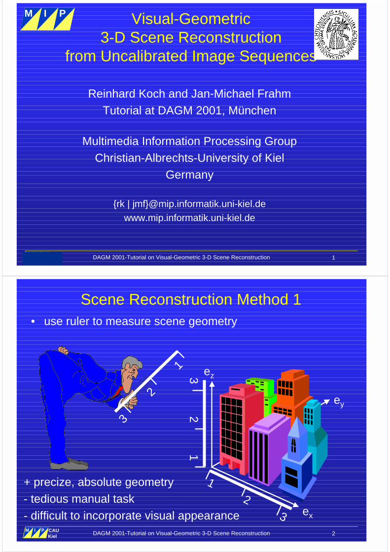
Visual-Geometric3-D Scene Reconstruction

from Uncalibrated Image Sequences

Reinhard Koch and Jan-Michael FrahmTutorial at DAGM 2001, München

Multimedia Information Processing GroupChristian-Albrechts-University of Kiel

Germany

{rk | jmf}@mip.informatik.uni-kiel.dewww.mip.informatik.uni-kiel.de

M I P


M I P




CAUKiel

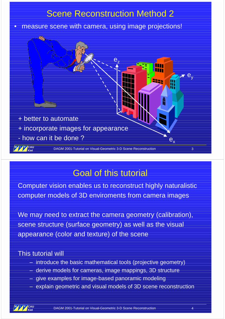
Scene Reconstruction Method 1• use ruler to measure scene geometry

ez

ey

ex

13

2

1

3

2

1

3

2

+ precize, absolute geometry- tedious manual task- difficult to incorporate visual appearance



CAUKiel

Scene Reconstruction Method 2• measure scene with camera, using image projections!

ez

ey

ex

+ better to automate+ incorporate images for appearance- how can it be done ?



CAUKiel

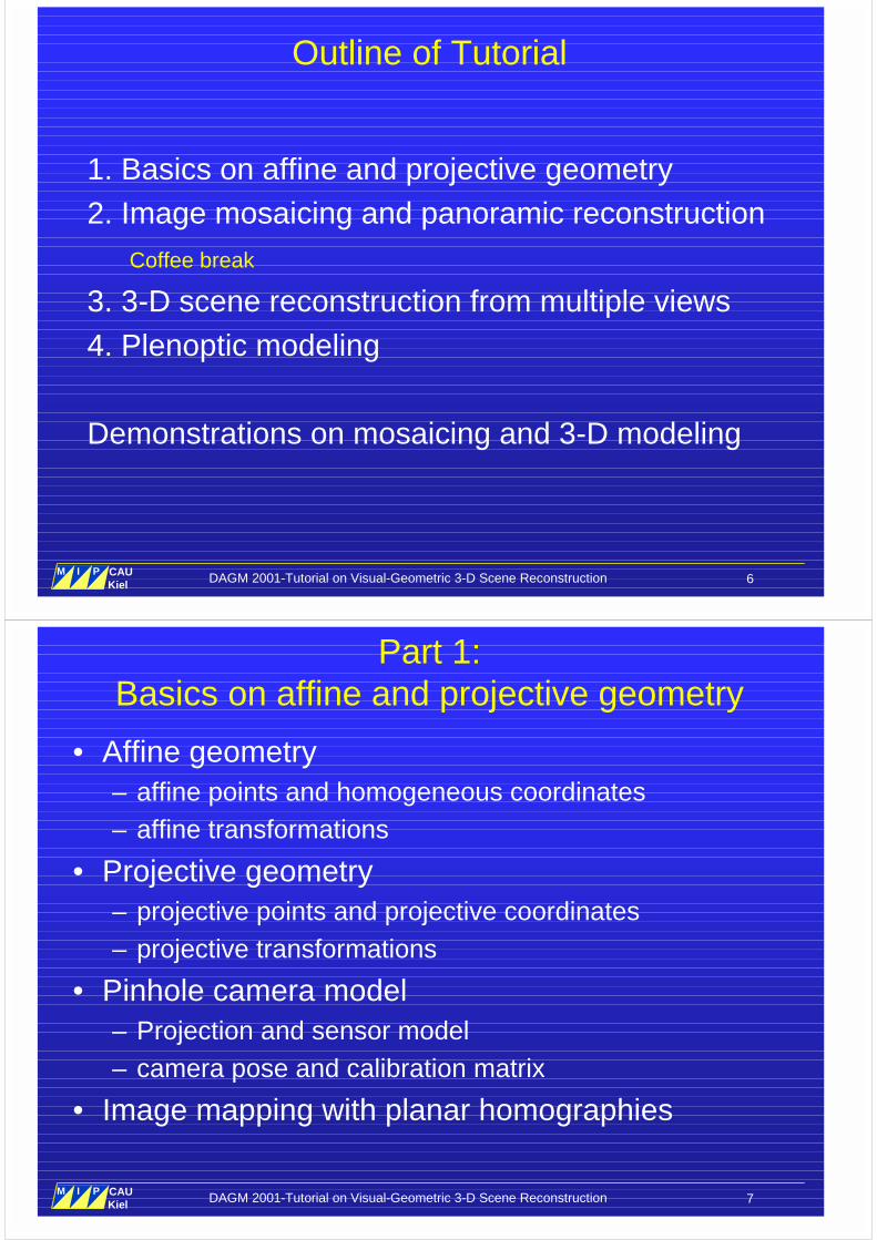
Goal of this tutorialComputer vision enables us to reconstruct highly naturalisticcomputer models of 3D enviroments from camera images

We may need to extract the camera geometry (calibration),scene structure (surface geometry) as well as the visualappearance (color and texture) of the scene

This tutorial will– introduce the basic mathematical tools (projective geometry)– derive models for cameras, image mappings, 3D structure– give examples for image-based panoramic modeling– explain geometric and visual models of 3D scene reconstruction



CAUKiel

Outline of Tutorial

1. Basics on affine and projective geometry2. Image mosaicing and panoramic reconstruction Coffee break

3. 3-D scene reconstruction from multiple views4. Plenoptic modeling

Demonstrations on mosaicing and 3-D modeling



CAUKiel

Part 1:Basics on affine and projective geometry

• Affine geometry– affine points and homogeneous coordinates– affine transformations

• Projective geometry– projective points and projective coordinates– projective transformations

• Pinhole camera model– Projection and sensor model– camera pose and calibration matrix

• Image mapping with planar homographies



CAUKiel

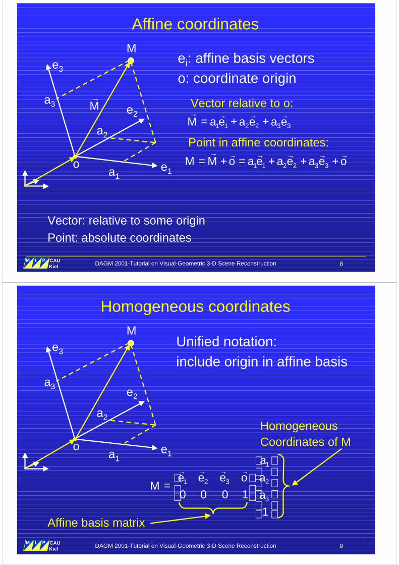
Affine coordinates

ei: affine basis vectorso: coordinate origin

e2

e3

e1o

M

1 1 2 2 3 3M a e a e a e= + +� � � �Vector relative to o:

a1

a3

a2

M�

1 1 2 2 3 3M M o a e a e a e o= + = + + +� � � � � �

Point in affine coordinates:

Vector: relative to some originPoint: absolute coordinates



CAUKiel

Homogeneous coordinates

e2

e3

e1o

MUnified notation:include origin in affine basis

=

� � � �1

1 2 3 2

30 0 0 1

1

a

e e e o aM

a

Affine basis matrix

HomogeneousCoordinates of M

a1

a3

a2



CAUKiel

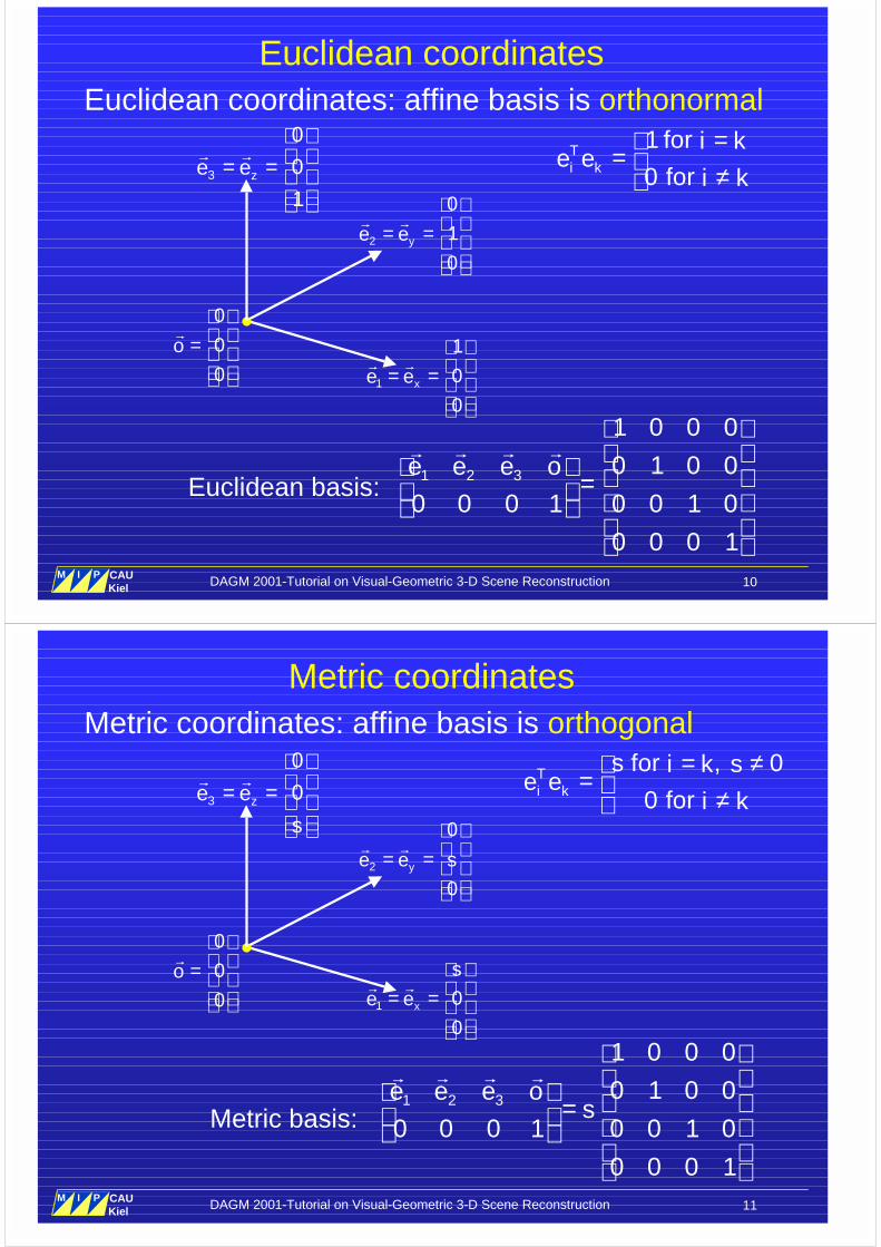
Euclidean coordinates: affine basis is orthonormal

Euclidean coordinates

1 for

0 for Ti k

i ke e

i k

== ≠

Euclidean basis:

1

1

0

0xe e

= =

� �

2

0

1

0ye e

= =

� �

3

0

0

1ze e

= =

� �

0

0

0

o

=

�

=

� � � �1 2 3

1 0 0 0

0 1 0 0

0 0 0 1 0 0 1 0

0 0 0 1

e e e o



CAUKiel

Metric coordinates: affine basis is orthogonal

Metric coordinates

s for , 0

0 for Ti k

i k se e

i k

= ≠= ≠

Metric basis:

1 0

0x

s

e e

= =

� �

2

0

0ye e s

= =

� �

3

0

0ze e

s

= =

� �

0

0

0

o

=

�

=

� � � �1 2 3

1 0 0 0

0 1 0 0

0 0 0 1 0 0 1 0

0 0 0 1

e e e os



CAUKiel

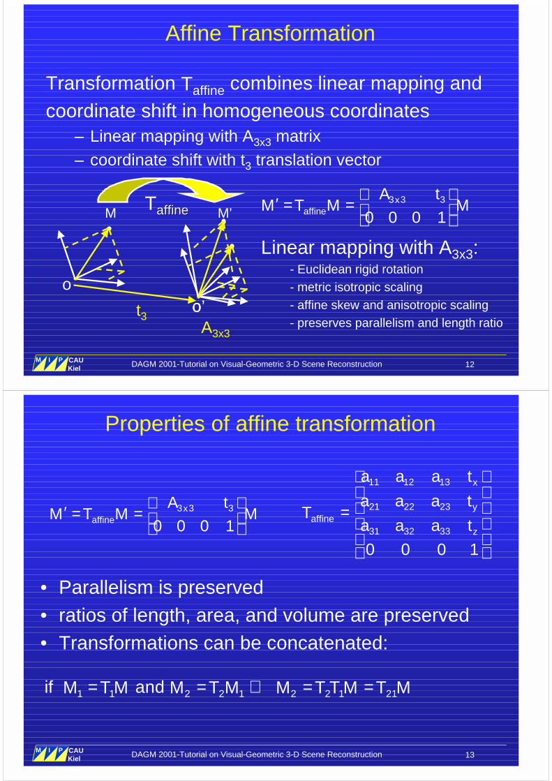
Affine Transformation

Transformation Taffine combines linear mapping andcoordinate shift in homogeneous coordinates

– Linear mapping with A3x3 matrix– coordinate shift with t3 translation vector

oo’

M M’Taffineaffine

t3

3 3 3

0 0 0 1x

affine

A tM T M M

′ = =

Linear mapping with A3x3:- Euclidean rigid rotation- metric isotropic scaling- affine skew and anisotropic scaling- preserves parallelism and length ratioA3x3

o



CAUKiel

Properties of affine transformation

• Parallelism is preserved• ratios of length, area, and volume are preserved• Transformations can be concatenated:

11 12 13

21 22 23

31 32 33

0 0 0 1

x

yaffine

z

a a a t

a a a tT

a a a t

=

3 3 3

0 0 0 1x

affine

A tM T M M

′ = =

1 1 2 2 1 2 2 1 21if and M T M M T M M T T M T M= = ⇒ = =



CAUKiel

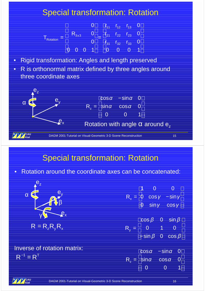
Special transformation: Rotation

• Rigid transformation: Angles and length preserved• R is orthonormal matrix defined by three angles around

three coordinate axes

11 12 13

3 3 21 22 23

31 32 33

0 0

0 0

0 0

0 0 0 1 0 0 0 1

xRotation

r r r

R r r rT

r r r

= =

ez

ey

ex

αcos sin 0

sin cos 0

0 0 1zR

α αα α

− =

Rotation with angle α around ez



CAUKiel

Special transformation: Rotation

• Rotation around the coordinate axes can be concatenated:

z y xR R R R=

ez

ey

ex

αβ

γ

cos sin 0

sin cos 0

0 0 1zR

α αα α

− =

cos 0 sin

0 1 0

sin 0 cosyR

β β

β β

= −

1 0 0

0 cos sin

0 sin cosxR γ γ

γ γ

= −

Inverse of rotation matrix:1 TR R− =



CAUKiel

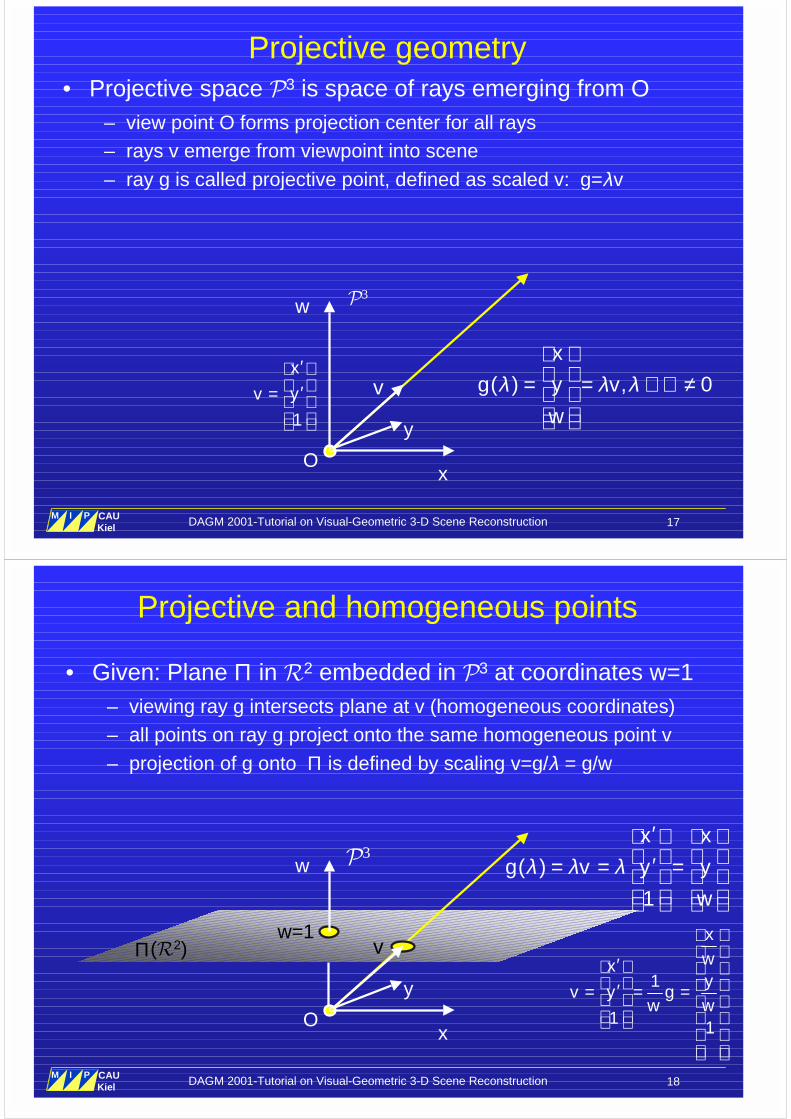
Projective geometry• Projective space �3 is space of rays emerging from O

– view point O forms projection center for all rays– rays v emerge from viewpoint into scene

– ray g is called projective point, defined as scaled v: g=λv

x

y

w �3

( ) , 0

x

g y v

w

λ λ λ = = ∈ ℜ ≠

v

O

1

x

v y

′ ′=



CAUKiel

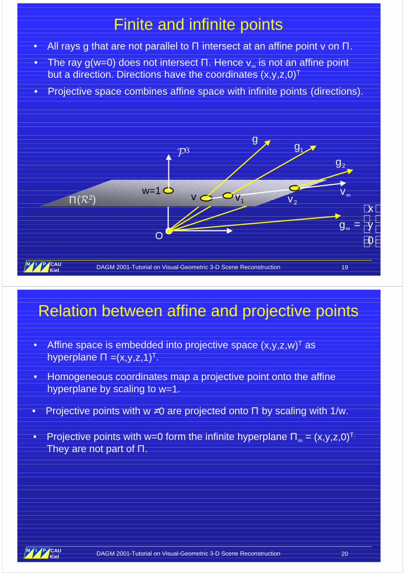
Projective and homogeneous points

• Given: Plane Π in �2 embedded in �3 at coordinates w=1– viewing ray g intersects plane at v (homogeneous coordinates)– all points on ray g project onto the same homogeneous point v

– projection of g onto Π is defined by scaling v=g/λ = g/w

w=1

�3( )

1

x x

g v y y

w

λ λ λ′

′= = =

1

1 1

xwxy

v y gw w

′ ′= = =

O

Π(�2)

w

x

v

y



CAUKiel

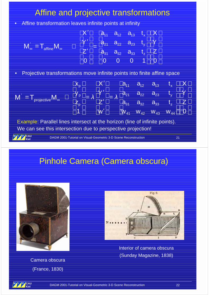
Finite and infinite points• All rays g that are not parallel to Π intersect at an affine point v on Π.

w=1

�3

O

vΠ(�2) 2v1v v∞

g1g

2g

0

x

g y∞

=

• The ray g(w=0) does not intersect Π. Hence v∞ is not an affine pointbut a direction. Directions have the coordinates (x,y,z,0)T

• Projective space combines affine space with infinite points (directions).



CAUKiel

Relation between affine and projective points

• Affine space is embedded into projective space (x,y,z,w)T ashyperplane Π =(x,y,z,1)T.

• Homogeneous coordinates map a projective point onto the affinehyperplane by scaling to w=1.

• Projective points with w ≠0 are projected onto Π by scaling with 1/w.

• Projective points with w=0 form the infinite hyperplane Π∞ = (x,y,z,0)T.

They are not part of Π.



CAUKiel

Affine and projective transformations• Affine transformation leaves infinite points at infinity

11 12 13

21 22 23

31 32 33

0 0 0 0 1 0

x

y

z

X a a a t X

Y a a a t Y

Z a a a t Z

′ ′ ⇒ = ′

'affineM T M∞ ∞=

• Projective transformations move infinite points into finite affine space

'projectiveM T M∞=

11 12 13

21 22 23

31 32 33

41 42 43 441 0

xp

yp

zp

a a a tx X X

a a a ty Y Y

a a a tz Z Z

w w w ww

λ λ

′ ′ ⇒ = = ′ ′

Example: Parallel lines intersect at the horizon (line of infinite points).We can see this intersection due to perspective projection!



CAUKiel

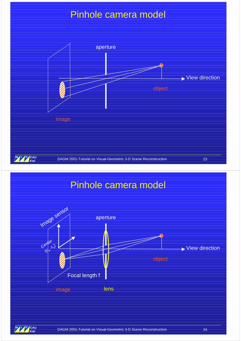
Pinhole Camera (Camera obscura)

Interior of camera obscura

(Sunday Magazine, 1838)Camera obscura

(France, 1830)



CAUKiel

aperture

image

object

View direction

Pinhole camera model



CAUKiel

Focal length f

aperture

image

object

View direction

lens

Image se

nsor

Center

(c x, c y

)

Pinhole camera model



CAUKiel

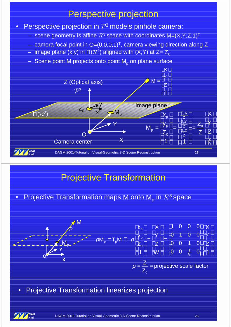
Perspective projection• Perspective projection in �3 models pinhole camera:

– scene geometry is affine �3 space with coordinates M=(X,Y,Z,1)T

– camera focal point in O=(0,0,0,1)T, camera viewing direction along Z– image plane (x,y) in Π(�2) aligned with (X,Y) at Z= Z0

– Scene point M projects onto point Mp on plane surface

X

Y

Z0

�3

O

pMΠ(�2)

Image plane

Camera center

Z (Optical axis)

1

X

YM

Z

=

0

0

0

0

0

0

1 1

Z Xp Z

Z Yp Z

p Z ZZ

ZZ

XxYy Z

MZZ Z

= = =

x

y



CAUKiel

Projective Transformation

• Projective Transformation maps M onto Mp in �3 space

0

01

1 0 0 0

0 1 0 0

0 0 1 0

0 0 01 1

p

pp p

z

x X X

y Y YM T M

Z Z Z

W

ρ ρ

= ⇒ = =

X

YO

M

pM

• Projective Transformation linearizes projection

0

projective scale factorZZ

ρ = =

ρ



CAUKiel

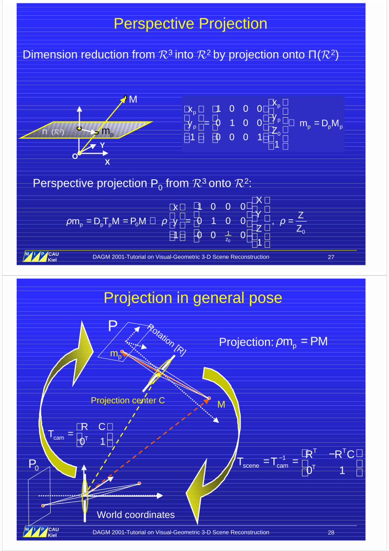
Perspective Projection

Dimension reduction from �3 into �2 by projection onto Π(�2)

X

YO

pm

M

Π (�2)

0

001

1 0 0 0

0 1 0 0 ,

1 0 0 01

p p p

z

Xx

Y Zm D T M P M y

Z Zρ ρ ρ

= = ⇒ = =

Perspective projection P0 from �3 onto �2:

0 0

1 0 0 0

0 1 0 0

0 0 1 0

1 0 0 0 1 1

p p

p p

x x

y y

Z Z

=

0 0

1 0 0 0

0 1 0 0

1 0 0 0

0 1 0

1 1

0

p p

p p

x x

y y

ZZ

=

0

1 0 0 0

0 1 0 0

1 0 0 0 11

pp

pp p p p

xx

yy m D M

Z

= ⇒ =



CAUKiel

Projection in general pose

Rotation [R]

Projection center C M

World coordinates

0P1

0 1

T T

scene cam T

R R CT T − −

= =

ρ =pm PMProjection:

0 1cam T

R CT

=

mp

P



CAUKiel

XY

Image centerc= (cx, cy)T

Projection center

Z (Optical axis)

Focal length Z0

Pixel scalef= (fx,fy)T

x

y

Pixel coordinatesm = (y,x)T

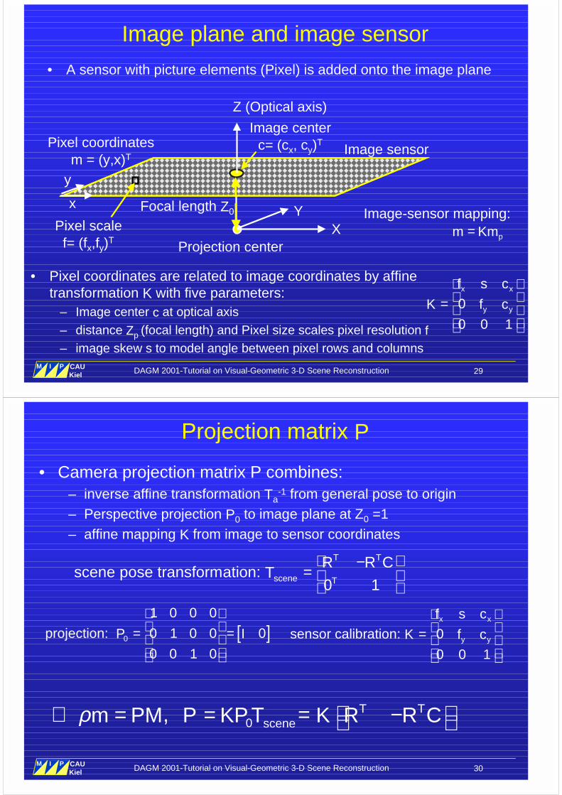
Image plane and image sensor

• A sensor with picture elements (Pixel) is added onto the image plane

Image sensor

pm Km=Image-sensor mapping:

0

0 0 1

x x

y y

f s c

K f c

=

• Pixel coordinates are related to image coordinates by affinetransformation K with five parameters:

– Image center c at optical axis– distance Zp (focal length) and Pixel size scales pixel resolution f– image skew s to model angle between pixel rows and columns



CAUKiel

Projection matrix P

• Camera projection matrix P combines:– inverse affine transformation Ta

-1 from general pose to origin– Perspective projection P0 to image plane at Z0 =1– affine mapping K from image to sensor coordinates

0, = T Tscenem PM P KP T K R R Cρ ⇒ = = −

[ ]0

1 0 0 0

projection: 0 1 0 0 0

0 0 1 0

P I

= =

scene pose transformation: 0 1

T T

scene T

R R CT

−=

sensor calibration: 0

0 0 1

x x

y y

f s c

K f c

=



CAUKiel

plane k

plane i

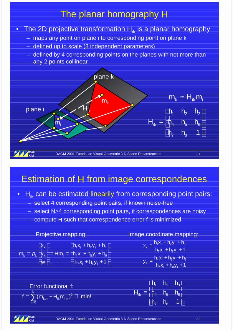
The planar homography H

• The 2D projective transformation Hik is a planar homography– maps any point on plane i to corresponding point on plane k– defined up to scale (8 independent parameters)– defined by 4 corresponding points on the planes with not more than

any 2 points collinear

km k ik im H m�

1 2 3

4 5 6

7 8 1ik

h h h

H h h h

h h

=

ikH

im



CAUKiel

Estimation of H from image correspondences

• Hik can be estimated linearily from corresponding point pairs:– select 4 corresponding point pairs, if known noise-free– select N>4 corresponding point pairs, if correspondences are noisy– compute H such that correspondence error f is minimized

1 2 3

4 5 6

7 8 1

k i i

k k k i i i

i i

x h x h y h

m y Hm h x h y h

w h x h y

ρ+ +

= = = + + + +

1 2 3

7 8

4 5 6

7 8

1

1

i ik

i i

i ik

i i

h x h y hx

h x h y

h x h y hy

h x h y

+ +=+ ++ +=+ +

Projective mapping: Image coordinate mapping:

Error functional f:2

, ,0

( ) min!N

k n ik i nn

f m H m=

= − ⇒∑1 2 3

4 5 6

7 8 1ik

h h h

H h h h

h h

=



CAUKiel

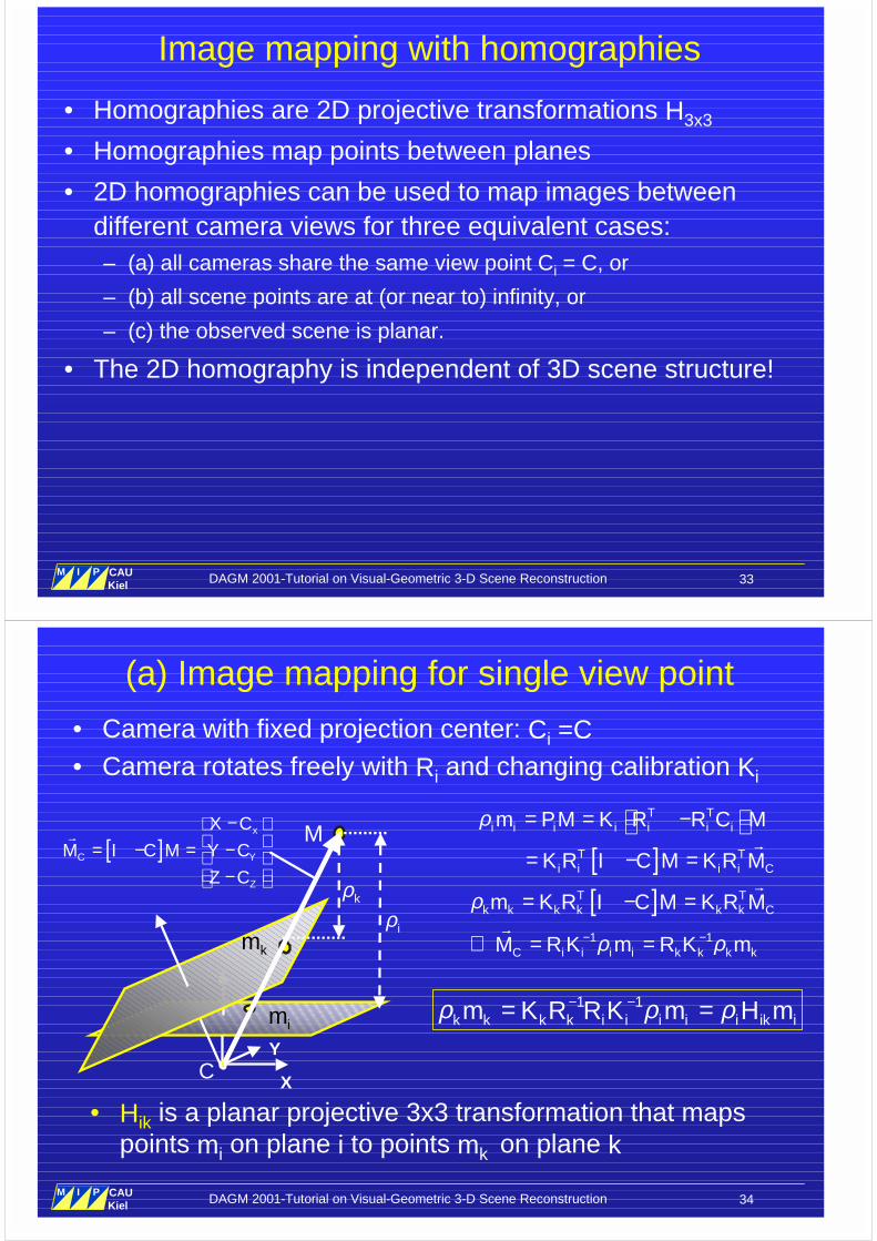
Image mapping with homographies

• Homographies are 2D projective transformations H3x3

• Homographies map points between planes

• 2D homographies can be used to map images betweendifferent camera views for three equivalent cases:– (a) all cameras share the same view point Ci = C, or

– (b) all scene points are at (or near to) infinity, or

– (c) the observed scene is planar.

• The 2D homography is independent of 3D scene structure!



CAUKiel

(a) Image mapping for single view point

• Camera with fixed projection center: Ci =C• Camera rotates freely with Ri and changing calibration Ki

[ ]

T Ti i i i i i i

T Ti i i i C

m PM K R R C M

K R I C M K R M

ρ = = − = − =

�

X

YC

im

M

km

[ ]ρ = − =�

T Tk k k k k k Cm K R I C M K R M

iρkρ

[ ]x

C Y

Z

X C

M I C M Y C

Z C

− = − = − −

�

1 1C i i i i k k k kM R K m R K mρ ρ− −⇒ = =�

1 1k k k k i i i i i ik im K R R K m H mρ ρ ρ− −= =

• Hik is a planar projective 3x3 transformation that mapspoints mi on plane i to points mk on plane k



CAUKiel

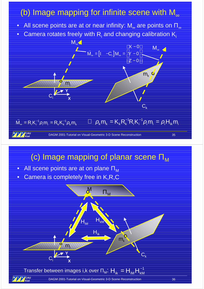
(b) Image mapping for infinite scene with M∞

• All scene points are at or near infinity: M∞ are points on Π∞

• Camera rotates freely with Ri and changing calibration Ki

X

YCi

im

M∞

km

[ ]0

0

0i

X

M I C M Y

Z∞ ∞

− = − = − −

�

1 1i i i i k k k kM R K m R K mρ ρ− −

∞ = =�

Ck

M∞

1 1k k k k i i i i i ik im K R R K m H mρ ρ ρ− −⇒ = =



CAUKiel

(c) Image mapping of planar scene ΠM

• All scene points are at on plane ΠM

• Camera is completely free in K,R,C

X

YCi

im

M

km

iMH

Ck

ΠM

ikH

kMH

1ik iM kMH H H −=Transfer between images i,k over ΠM:



CAUKiel

Part 2:Mosaicing and Panoramic Images

• why mosaicing?

• geometries constraints for mosaicing

• mosaicing

• projective mainfolds

• stereo mosaicing



CAUKiel

Why mosaicing?

• cameras field of view is always smaller thanhuman field of view

• large objects can‘t be captured in a single picture

Solutions

• devices with wide field of view

- fish-eye lenses (distortions, decreases quality)

- hyper- and parabolic optical devices (lowerresolution)

• image mosaicing



CAUKiel

What is mosaicing?

definition of mosaicing : Matching multipleimages by aligning and pasting images to awilder field of view image. Features that continueover the images must be "zipped" together, andthe frame edges dissolved.

mosaicing

Kang et. al. (ICPR 2000)



CAUKiel

Geometries of mosaic aquisition

rotatingcamera

planar scene

translating and rotatingcamera

arbitrary scene



CAUKiel

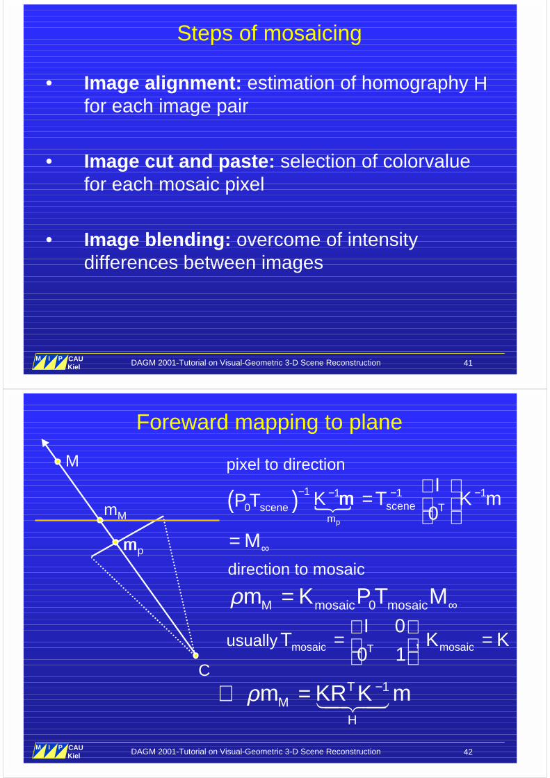
Steps of mosaicing

• Image alignment: estimation of homography Hfor each image pair

• Image cut and paste: selection of colorvaluefor each mosaic pixel

• Image blending: overcome of intensitydifferences between images



CAUKiel

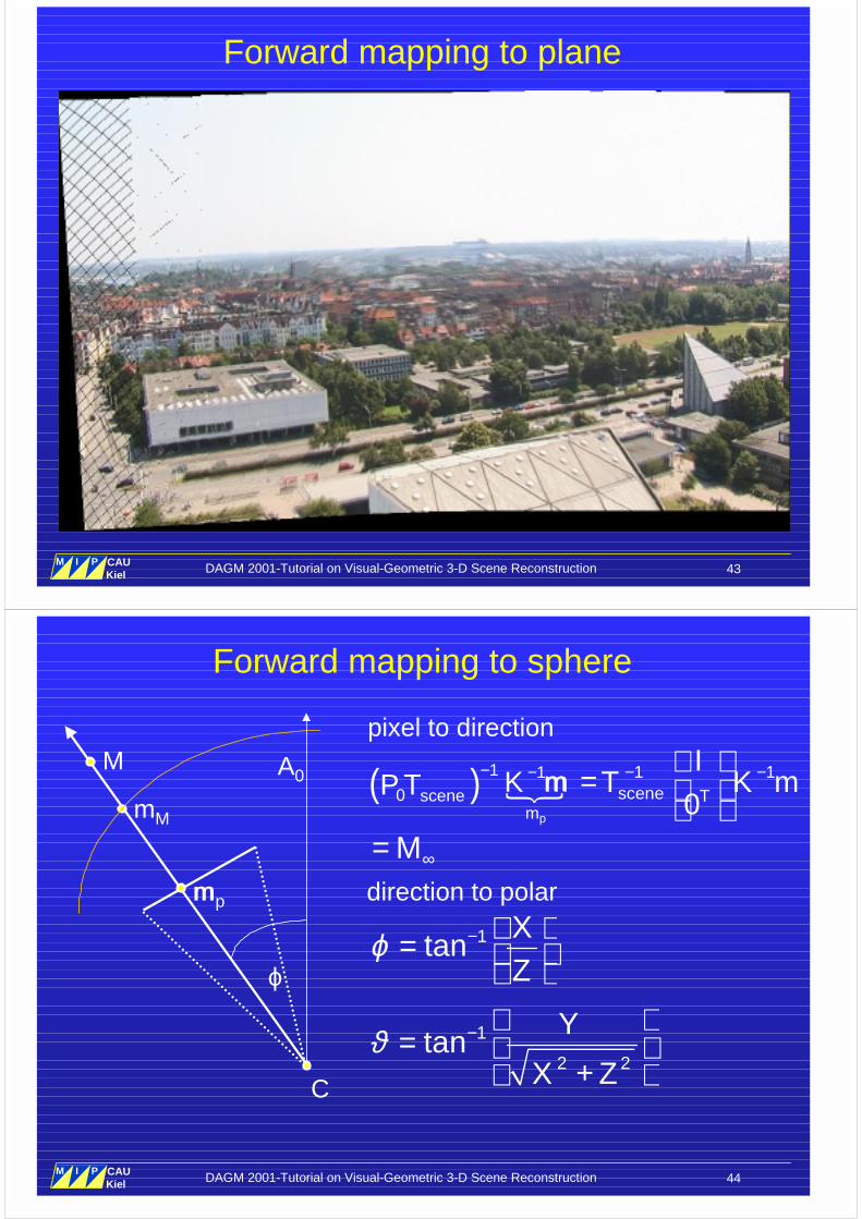
Foreward mapping to plane

C

M

mmp

mM�

−1

pm

K m( )−1

0 sceneP T m − − =

1 1

0scene T

IT K m

∞= M

ρ ∞= 0M mosaic mosaicm K P T M

pixel to direction

direction to mosaic

usually

= =

0,

0 1mosaic mosaicT

IT K K

ρ −⇒ = ��1T

MH

m KR K m



CAUKiel

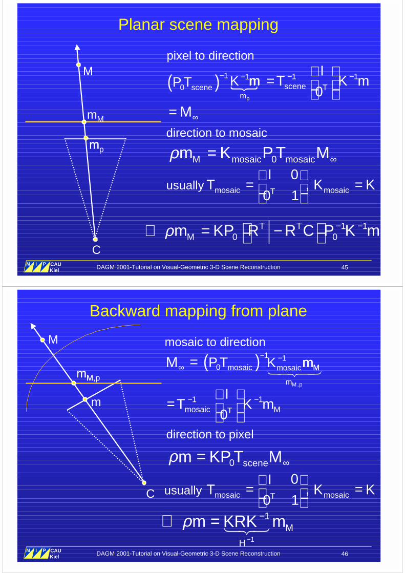
Forward mapping to plane



CAUKiel

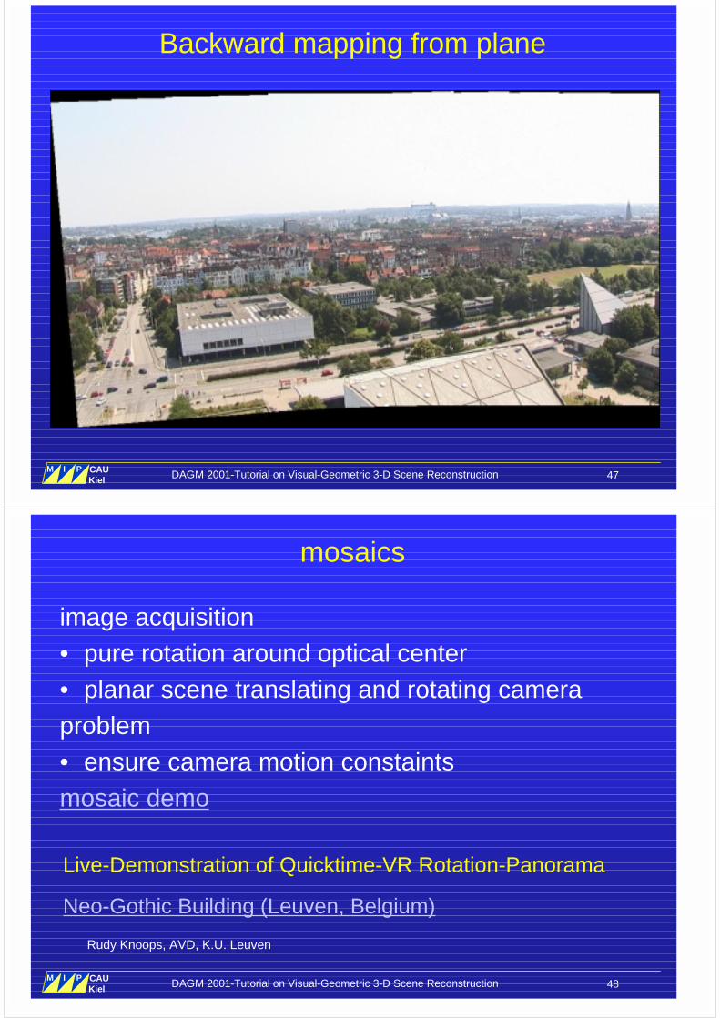
Forward mapping to sphere

C

M

mmp

mM

A0

ϕ

�

−1

pm

K m( )−1


1 1

0scene T

IT K m

∞= M

pixel to direction

direction to polar

ϑ − =

+ 1

2 2tan

Y

X Z

ϕ − = 1tan

XZ



CAUKiel

Planar scene mapping

M

m

mM

�

−1

pm

K m( )−1


1 1

0scene T

IT K m

∞= M

ρ ∞= 0M mosaic mosaicm K P T M

pixel to direction

direction to mosaic

usually

= =

0,

0 1mosaic mosaicT

IT K K

ρ − − ⇒ = − 1 1

0 0T T

Mm KP R R C P K m

mp

C



CAUKiel

Backward mapping from plane

mM,p

C

M

m

mM

−

��,

1

M p

mosaic M

m

K m( )−1

0 mosaicP T Mm

− − =

1 1

0mosaic MT

IT K m

∞ =M

ρ ∞= 0 scenem KP T M

mosaic to direction

direction to pixel

usually

= =

0,

0 1mosaic mosaicT

IT K K

ρ−

−⇒ = ��1

1M

H

m KRK m



CAUKiel

Backward mapping from plane



CAUKiel

mosaics

image acquisition• pure rotation around optical center• planar scene translating and rotating cameraproblem• ensure camera motion constaintsmosaic demo

Live-Demonstration of Quicktime-VR Rotation-Panorama

Neo-Gothic Building (Leuven, Belgium)

Rudy Knoops, AVD, K.U. Leuven



CAUKiel

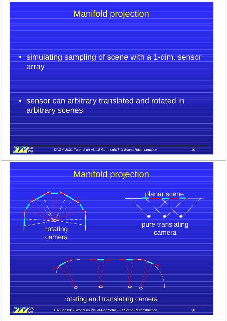
Manifold projection

• simulating sampling of scene with a 1-dim. sensorarray

• sensor can arbitrary translated and rotated inarbitrary scenes



CAUKiel

Manifold projection

rotatingcamera

planar scene

pure translatingcamera

rotating and translating camera



CAUKiel

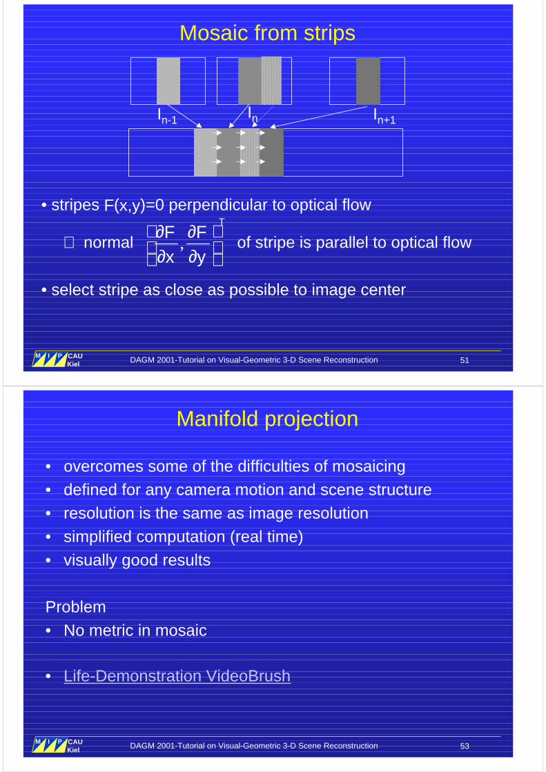
Mosaic from strips

In-1 In In+1

• stripes F(x,y)=0 perpendicular to optical flow

⇒ normal of stripe is parallel to optical flow, ∂ ∂ ∂ ∂

F Fx y

T

• select stripe as close as possible to image center



CAUKiel

Manifold projection

• overcomes some of the difficulties of mosaicing• defined for any camera motion and scene structure• resolution is the same as image resolution• simplified computation (real time)• visually good results

Problem• No metric in mosaic

• Life-Demonstration VideoBrush



CAUKiel

Stereo mosaics

• multiple viewpoint panorama

• for each eye a seperate multiple viewpointpanorama

• constructed from one rotating camera



CAUKiel

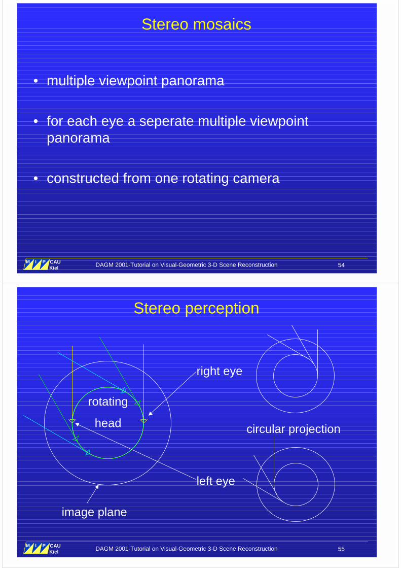
Stereo perception

rotating

head

left eye

right eye

circular projection

image plane



CAUKiel

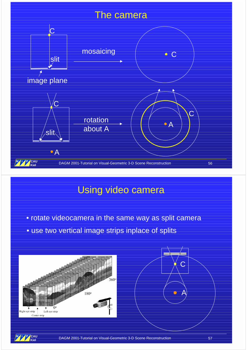
slit

C

A

The camera

image plane

C

Cmosaicingslit

Crotationabout A A



CAUKiel

A

C

Using video camera

• rotate videocamera in the same way as split camera

• use two vertical image strips inplace of splits



CAUKiel

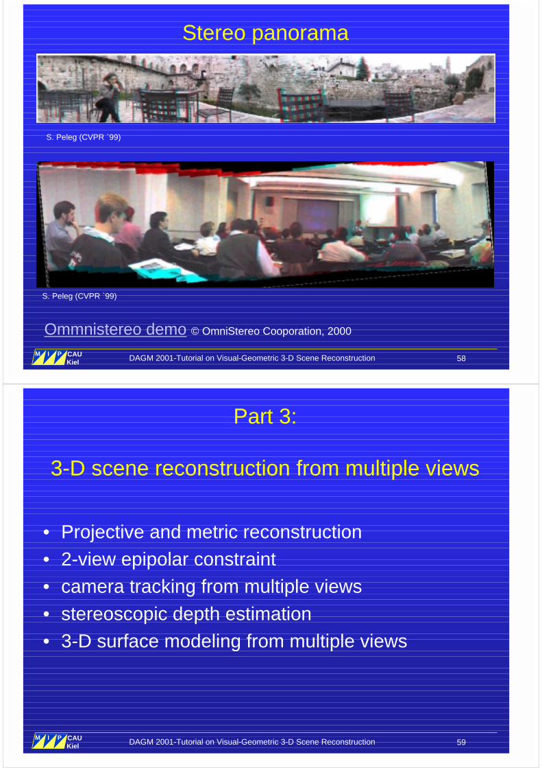
Stereo panorama

S. Peleg (CVPR `99)

S. Peleg (CVPR `99)

Ommnistereo demo © OmniStereo Cooporation, 2000



CAUKiel

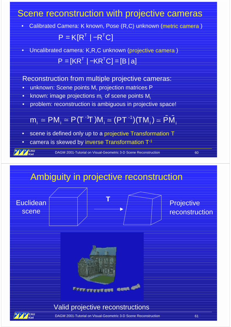
Part 3:

3-D scene reconstruction from multiple views

• Projective and metric reconstruction• 2-view epipolar constraint• camera tracking from multiple views• stereoscopic depth estimation• 3-D surface modeling from multiple views



CAUKiel

• Calibrated Camera: K known, Pose (R,C) unknown (metric camera )

[ | ]T TP K R R C= −

• Uncalibrated camera: K,R,C unknown (projective camera )

[ | ] [ | ]T TP KR KR C B a= − =

Scene reconstruction with projective cameras

Reconstruction from multiple projective cameras:• unknown: Scene points M, projection matrices P• known: image projections mi of scene points Mi

• problem: reconstruction is ambiguous in projective space!

�i im PM

• scene is defined only up to a projective Transformation T• camera is skewed by inverse Transformation T-1

�-1( ) iP T T M �

-1( )( )iPT TM � �� iPM



CAUKiel

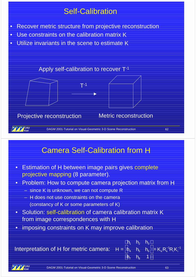
Ambiguity in projective reconstruction

TEuclideanscene

Projectivereconstruction

Valid projective reconstructions



CAUKiel

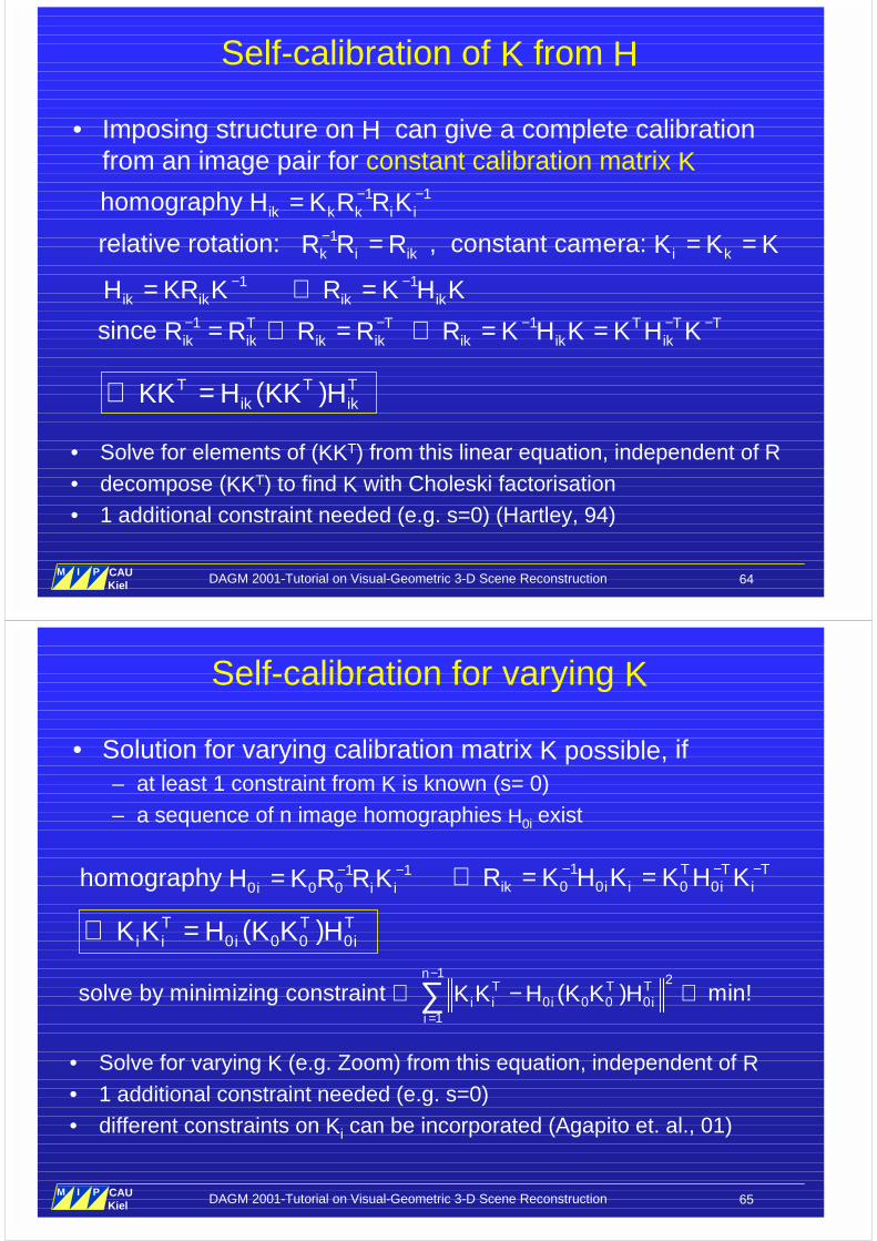
Self-Calibration

T-1

Metric reconstructionProjective reconstruction

Apply self-calibration to recover T-1

• Recover metric structure from projective reconstruction• Use constraints on the calibration matrix K• Utilize invariants in the scene to estimate K



CAUKiel

Camera Self-Calibration from H

• Estimation of H between image pairs gives completeprojective mapping (8 parameter).

• Problem: How to compute camera projection matrix from H– since K is unknown, we can not compute R– H does not use constraints on the camera (constancy of K or some parameters of K)

• Solution: self-calibration of camera calibration matrix Kfrom image correspondences with H

• imposing constraints on K may improve calibration

1 2 31 1

4 5 6

7 8 1k k i i

h h h

H h h h K R R K

h h

− −

= =

Interpretation of H for metric camera:



CAUKiel

Self-calibration of K from H

• Imposing structure on H can give a complete calibrationfrom an image pair for constant calibration matrix K

1 1homography ik k k i iH K R R K− −=

1ik ikH KR K −=

1relative rotation: , constant camera: k i ik i kR R R K K K− = = =

1since T Tik ik ik ikR R R R− −= ⇒ =

1ik ikR K H K−⇒ =

1 T T Tik ik ikR K H K K H K− − −⇒ = =

( ) T T Tik ikKK H KK H⇒ =

• Solve for elements of (KKT) from this linear equation, independent of R• decompose (KKT) to find K with Choleski factorisation• 1 additional constraint needed (e.g. s=0) (Hartley, 94)



CAUKiel

Self-calibration for varying K

• Solution for varying calibration matrix K possible, if– at least 1 constraint from K is known (s= 0)– a sequence of n image homographies H0i exist

1 10 0 0homography i i iH K R R K− −= 1

0 0 0 0T T T

ik i i i iR K H K K H K− − −⇒ = =

0 0 0 0( ) T T Ti i i iK K H K K H⇒ =

• Solve for varying K (e.g. Zoom) from this equation, independent of R• 1 additional constraint needed (e.g. s=0)• different constraints on Ki can be incorporated (Agapito et. al., 01)

1 2

0 0 0 01

solve by minimizing constraint ( ) min! n

T T Ti i i i

i

K K H K K H−

=

⇒ − ⇒∑



CAUKiel

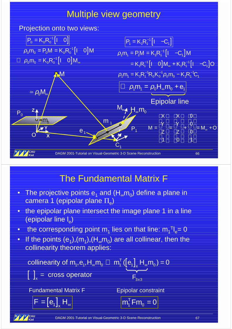
Multiple view geometryProjection onto two views:

0

0

0

1 0 1

X X

Y YM M O

Z Z ∞

= = + = +

X

Y

O

0m

M

Z

C1

1mP0

P1

[ ]10 0 0 0P K R I−=

[ ]11 1 1 1 1 1m PM K R I C Mρ −= = −[ ]1

0 0 0 0 0 0m P M K R I Mρ −= =[ ]1

1 1 1 1P K R I C−= −

[ ]10 0 0 0 0m K R I Mρ −

∞⇒ =

0Mρ ∞�

[ ] [ ]1 11 1 1 1 10K R I M K R I C O− −

∞= + −

M∞

1 1 11 1 1 1 0 0 0 0 1 1 1m K R R K m K R Cρ ρ− − −= −

1 1 0 0 1m H m eρ ρ ∞⇒ = +

1e

0H m∞

Epipolar line



CAUKiel

The Fundamental Matrix F• The projective points e1 and (H∞m0) define a plane in

camera 1 (epipolar plane �e)

• the epipolar plane intersect the image plane 1 in a line(epipolar line le)

• the corresponding point m1 lies on that line: m1Tle= 0

• If the points (e1),(m1),(H∞m0) are all collinear, then thecollinearity theorem applies:

[ ][ ]

1 1 0 1 1 0collinearity of , , ( ) 0

cross operator

T

x

x

m e H m m e H m∞ ∞⇒ =

=

1 0 0Tm Fm =[ ]1 xF e H∞=

Fundamental Matrix F Epipolar constraint

3 3xF



CAUKiel

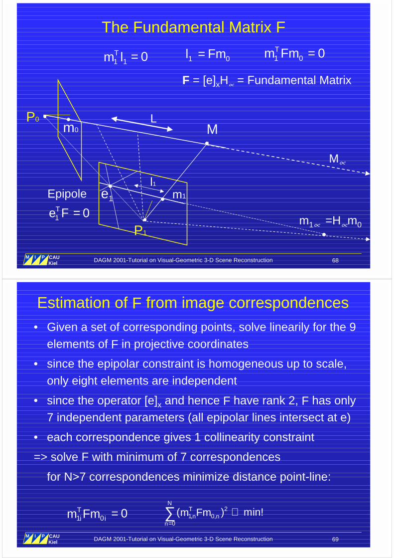
The Fundamental Matrix F

P0

m0

1 1 0Tm l =

L

l1

M

m1

M�

P1

1 0l Fm=

m1� =H�

m0

1 0 0Tm Fm =

Epipole e1

F = [e]xH� = Fundamental Matrix

1 0Te F =



CAUKiel

Estimation of F from image correspondences

• Given a set of corresponding points, solve linearily for the 9elements of F in projective coordinates

• since the epipolar constraint is homogeneous up to scale,only eight elements are independent

• since the operator [e]x and hence F have rank 2, F has only7 independent parameters (all epipolar lines intersect at e)

• each correspondence gives 1 collinearity constraint

=> solve F with minimum of 7 correspondences

for N>7 correspondences minimize distance point-line:

1 0 0Ti im Fm = 2

1, 0,0

( ) min!N

Tn n

n

m Fm=

⇒∑



CAUKiel

Estimation of P from F• From F we can obtain a camera projection matrix pair:

– Set P0 to identity

– compute P1 from F (up to projective transformation)

– reduce projective skew by initial estimate of K to obtain a quasi-euclidean estimate (Pollefeys et.al., ‘98)

– compute self-calibration to obtain metric K similar to self-calibrationfrom H (Pollefeys et.al, ‘99, Fusiello ‘00)

0 [ | 0]P I=

1 1 1[[ ] | ]TxP e F e a e= +

Fundamental matrix ↔ Projective camera

1 0 0Tm Fm =

1 0Te F =



CAUKiel

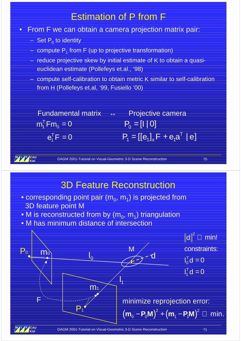
3D Feature Reconstruction• corresponding point pair (m0, m1) is projected from 3D feature point M• M is reconstructed from by (m0, m1) triangulation• M has minimum distance of intersection

P1

m0

m1

P0

F

1l

0

2

1

constraints

in

0

!

:

0

m

T

Td

d

l d

l

⇒

=

=

0l dM

( ) ( )2 2

0 0 1 1

minimize reprojection error:

min.− + − ⇒m P M m PM



CAUKiel

Multi View Tracking• 2D match: Image correspondence (m1, mi)

P1

m0

m1

P0

Pi

M

3D match

2D match

mi

• 3D match: Correspondence transfer (mi, M) via P1

• 3D Pose estimation of Pi with mi - Pi M => min.

2

,0 0

Minimize lobal reprojection error: min!N K

k i i ki k

m PM= =

− ⇒∑∑



CAUKiel

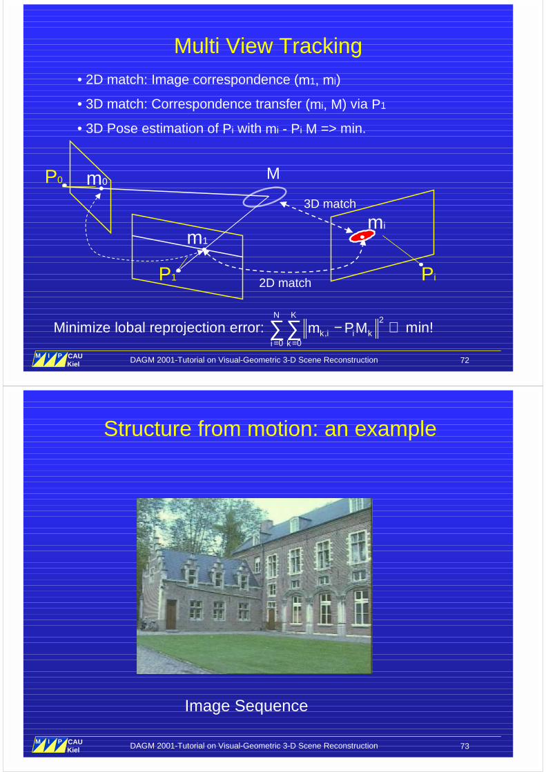
Structure from motion: an example

Image Sequence



CAUKiel

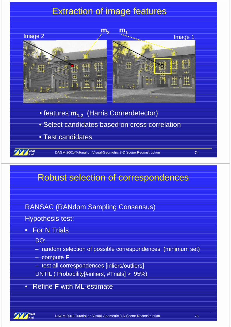
Extraction of image features

• features m1,2 (Harris Cornerdetector)

Image 2 Image 1m2 m1

• Select candidates based on cross correlation

• Test candidates



CAUKiel

Robust selection of correspondences

RANSAC (RANdom Sampling Consensus)

Hypothesis test:

• For N Trials

DO:

– random selection of possible correspondences (minimum set)– compute F– test all correspondences [inliers/outliers]UNTIL ( Probability[#inliers, #Trials] > 95%)

• Refine F with ML-estimate



CAUKiel

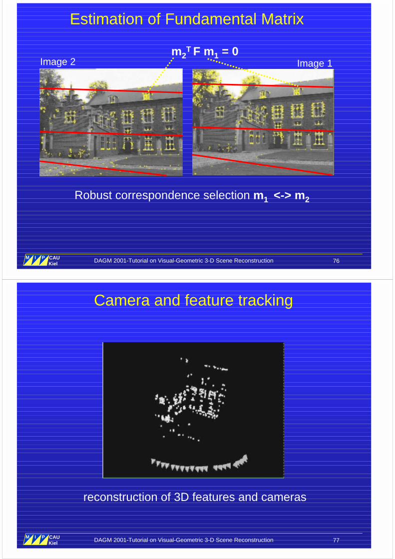
Estimation of Fundamental Matrix

Image 2 Image 1m2

T F m1 = 0

Robust correspondence selection m1 <-> m2



CAUKiel

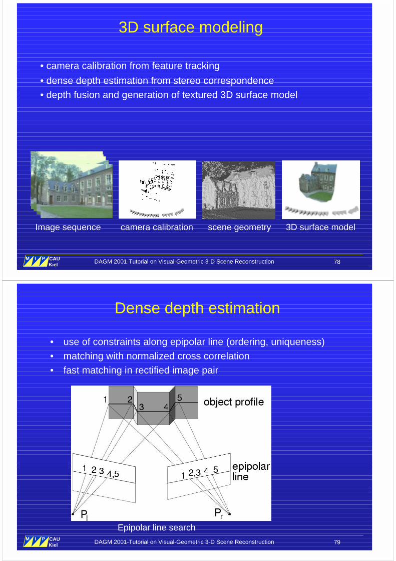
Camera and feature tracking

reconstruction of 3D features and cameras



CAUKiel

3D surface modeling

Image sequence camera calibration scene geometry 3D surface model

• camera calibration from feature tracking

• dense depth estimation from stereo correspondence• depth fusion and generation of textured 3D surface model



CAUKiel

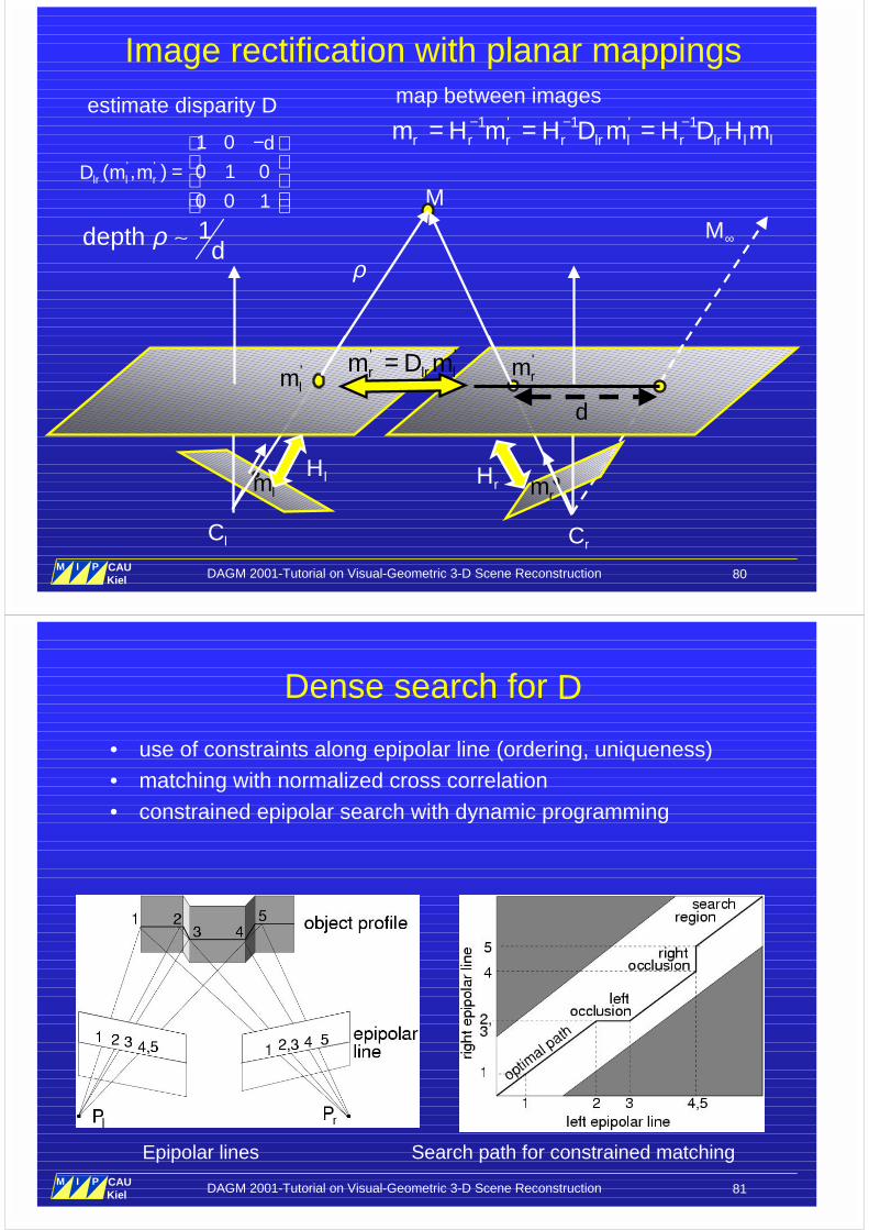
Dense depth estimation

• use of constraints along epipolar line (ordering, uniqueness)• matching with normalized cross correlation• fast matching in rectified image pair

Epipolar line search



CAUKiel

Image rectification with planar mappings

M

lCrC

M∞

lH

' 'r lr lm D m=

rH

' '

1 0

( , ) 0 1 0

0 0 1lr l r

d

D m m

− =

estimate disparity D1 ' 1 ' 1

r r r r lr l r lr l lm H m H D m H D H m− − −= = =

'rm'

lmd

lmrm

map between images

ρ1depth dρ �



CAUKiel

Dense search for D

• use of constraints along epipolar line (ordering, uniqueness)• matching with normalized cross correlation• constrained epipolar search with dynamic programming

Epipolar lines Search path for constrained matching



CAUKiel

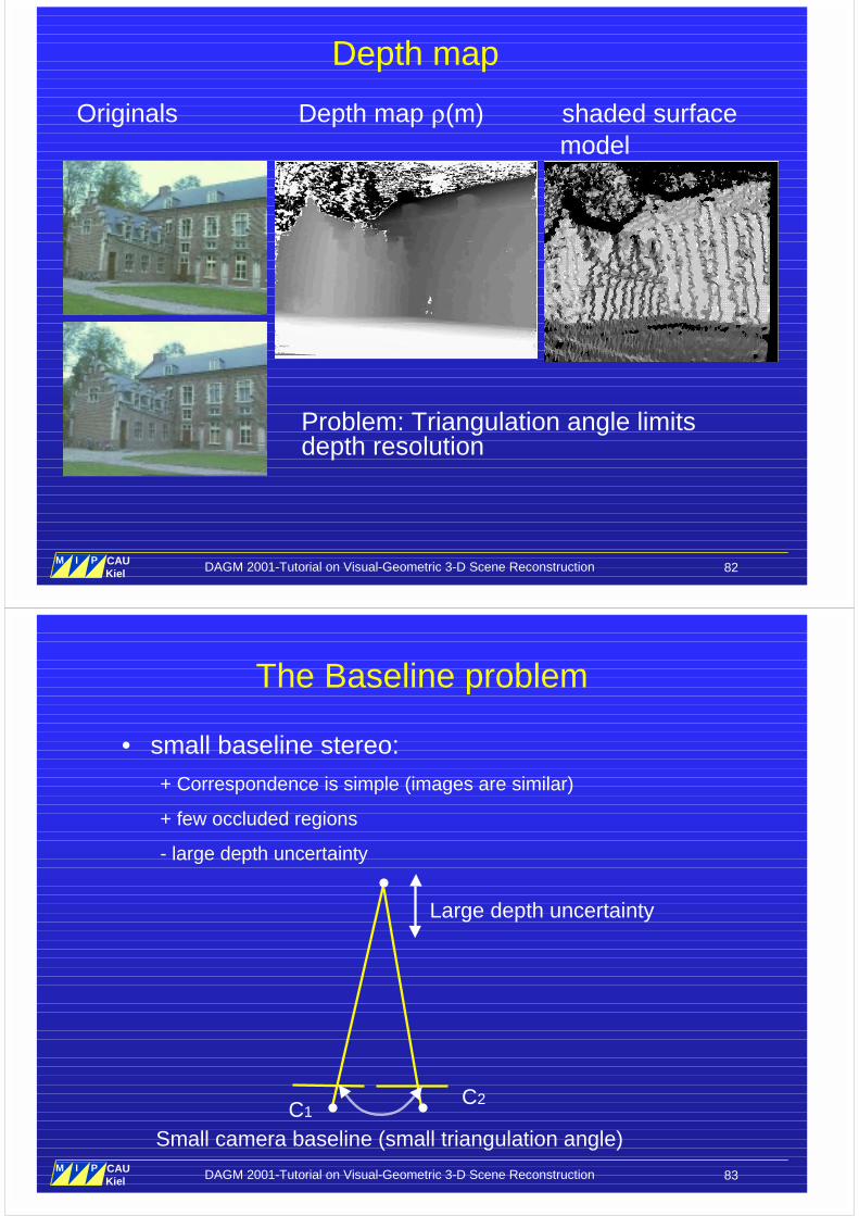
Depth map

Originals Depth map �(m) shaded surface model

Problem: Triangulation angle limitsdepth resolution



CAUKiel

The Baseline problem

• small baseline stereo:+ Correspondence is simple (images are similar)

+ few occluded regions

- large depth uncertainty

Large depth uncertainty

Small camera baseline (small triangulation angle)

C2C1



CAUKiel

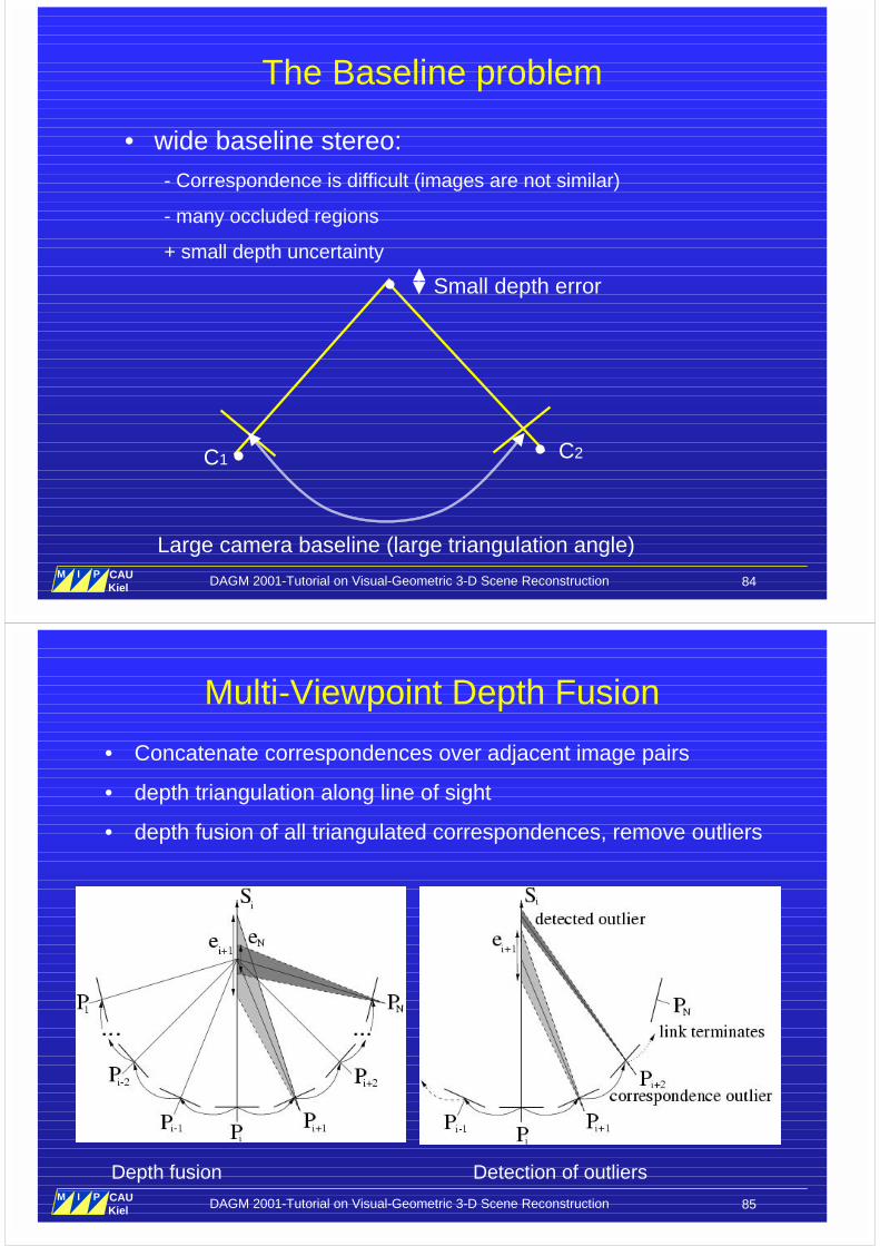
The Baseline problem

• wide baseline stereo:- Correspondence is difficult (images are not similar)

- many occluded regions

+ small depth uncertainty

Large camera baseline (large triangulation angle)

Small depth error

C1 C2



CAUKiel

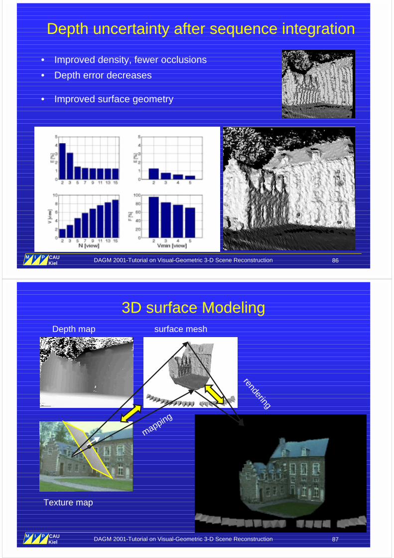
Multi-Viewpoint Depth Fusion

Detection of outliers

• Concatenate correspondences over adjacent image pairs

• depth triangulation along line of sight

• depth fusion of all triangulated correspondences, remove outliers

Depth fusion



CAUKiel

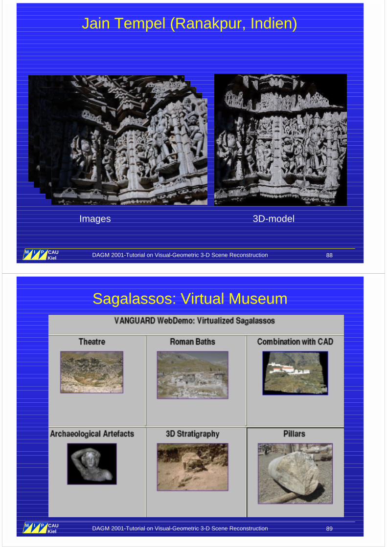
Depth uncertainty after sequence integration

• Improved density, fewer occlusions

• Depth error decreases

• Improved surface geometry



CAUKiel

3D surface ModelingDepth map surface mesh

Texture map

mapping

rendering



CAUKiel

Jain Tempel (Ranakpur, Indien)

Images 3D-model



CAUKiel

Sagalassos: Virtual Museum



CAUKiel

Open Questions from geometric modeling

• How much geometry is really needed for visualisation ?• Trade-off: modeling vs. texture mapping (reflectance,

microstructure)• how can we model surface reflections ?• How can we efficiently store and render the scenes ?



CAUKiel

Part 4:Plenoptic Modeling

• The lightfield• depth-dependent view interpolation• The uncalibrated Lumigraph• Visual-geometric modeling: view-dependent interpolation

and texture mapping



CAUKiel

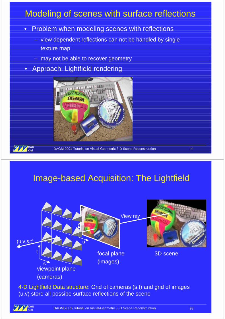
Modeling of scenes with surface reflections

• Problem when modeling scenes with reflections

– view dependent reflections can not be handled by single

texture map

– may not be able to recover geometry

• Approach: Lightfield rendering



CAUKiel

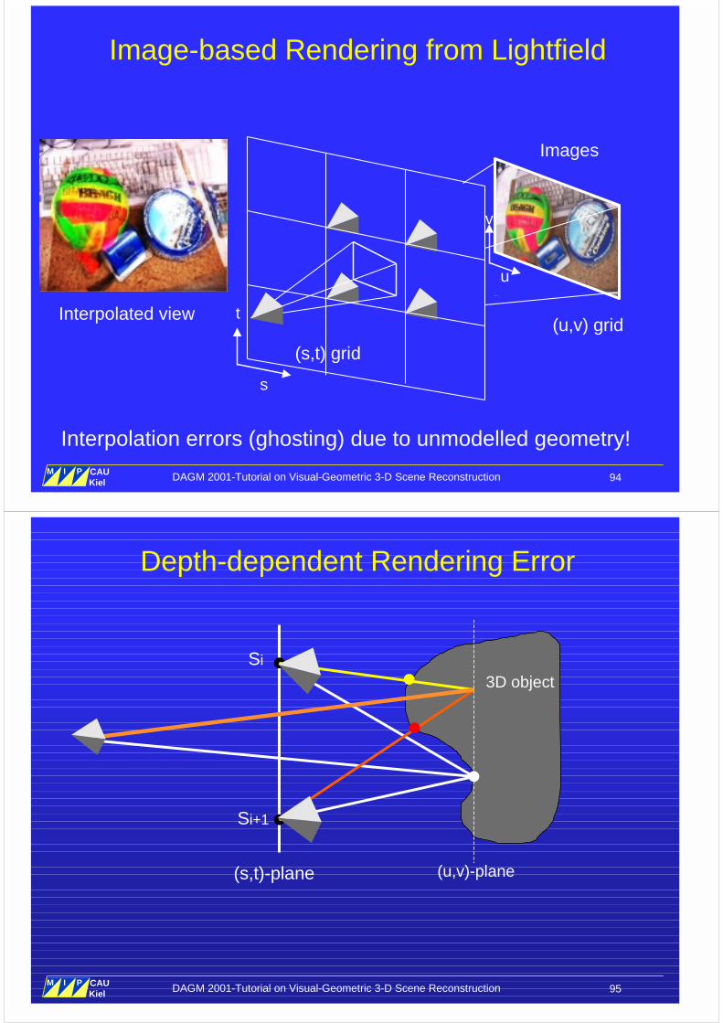
Image-based Acquisition: The Lightfield

viewpoint plane(cameras)

focal plane(images)

3D scene

4-D Lightfield Data structure: Grid of cameras (s,t) and grid of images(u,v) store all possibe surface reflections of the scene

u

v

View ray

s

t

(u,v,s,t)



CAUKiel

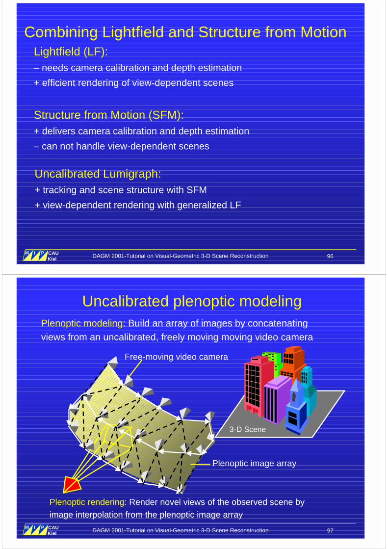
Image-based Rendering from Lightfield

(s,t) grid

s

tInterpolated view

u

v

(u,v) grid

Images

Interpolation errors (ghosting) due to unmodelled geometry!



CAUKiel

Depth-dependent Rendering Error

(s,t)-plane (u,v)-plane

3D object

Si+1

Si



CAUKiel

Combining Lightfield and Structure from MotionLightfield (LF):– needs camera calibration and depth estimation

+ efficient rendering of view-dependent scenes

Structure from Motion (SFM):+ delivers camera calibration and depth estimation

– can not handle view-dependent scenes

Uncalibrated Lumigraph:+ tracking and scene structure with SFM

+ view-dependent rendering with generalized LF



CAUKiel

Uncalibrated plenoptic modeling

3-D Scene

Plenoptic modeling: Build an array of images by concatenatingviews from an uncalibrated, freely moving moving video camera

Plenoptic rendering: Render novel views of the observed scene byimage interpolation from the plenoptic image array

Free-moving video camera

Plenoptic image array



CAUKiel

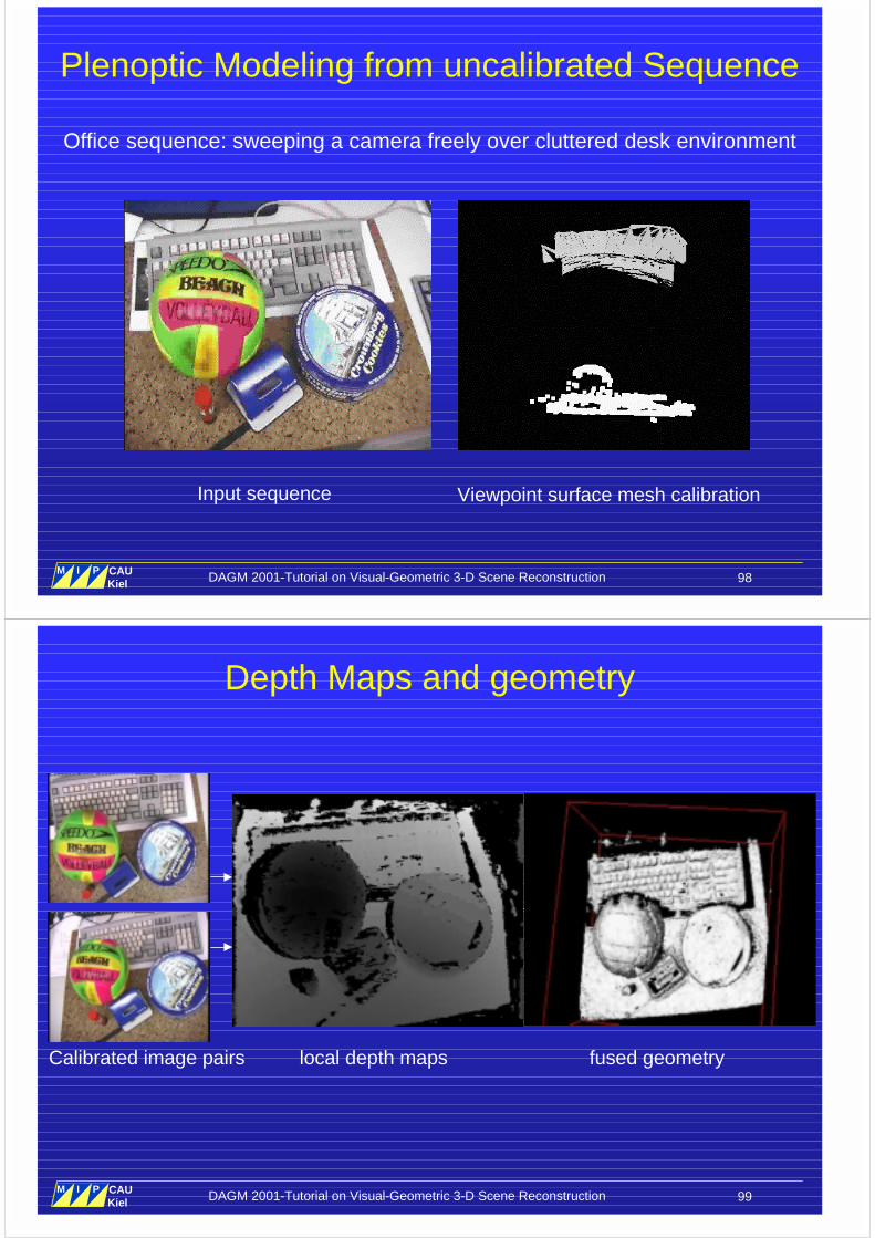
Plenoptic Modeling from uncalibrated Sequence

Office sequence: sweeping a camera freely over cluttered desk environment

Input sequence Viewpoint surface mesh calibration



CAUKiel

Depth Maps and geometry

Calibrated image pairs local depth maps fused geometry



CAUKiel

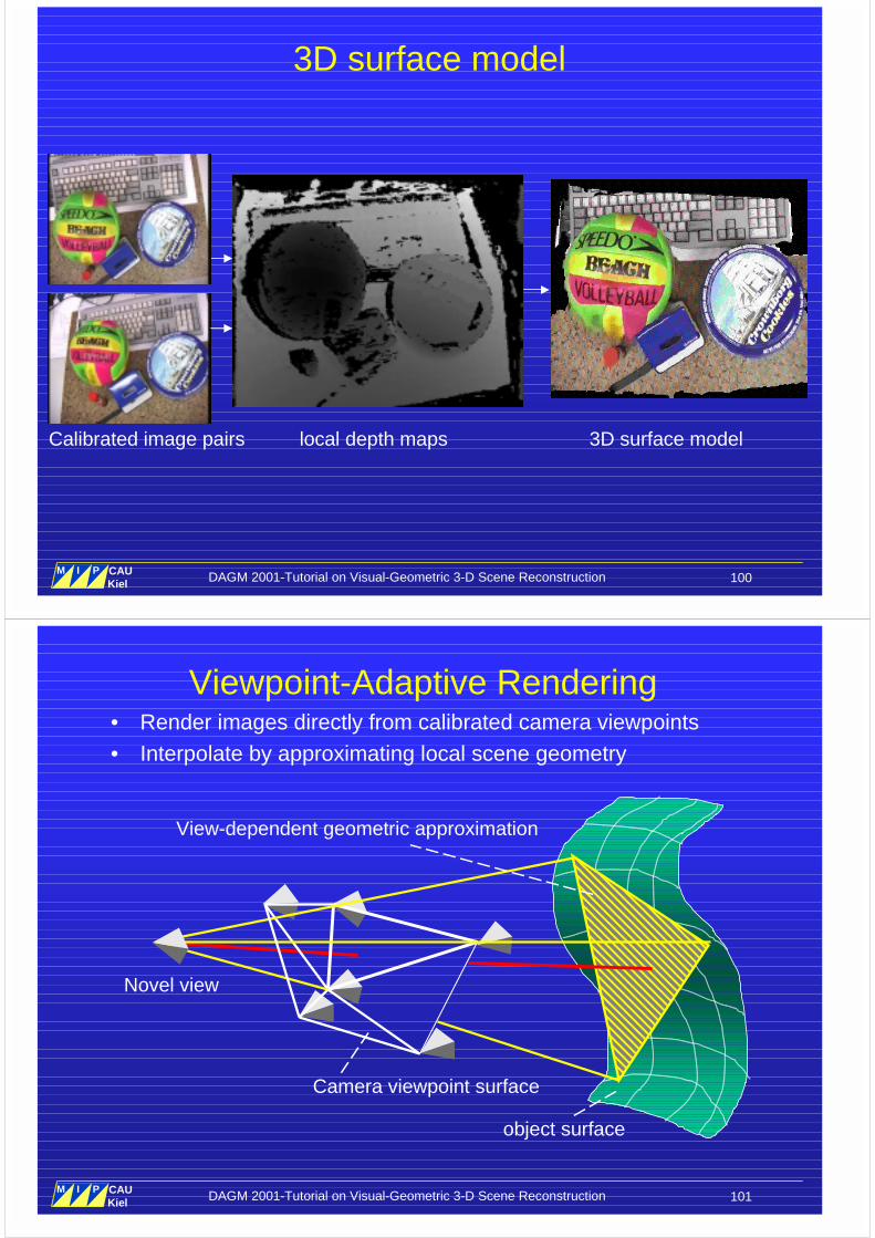
3D surface model

Calibrated image pairs local depth maps 3D surface model



CAUKiel

Viewpoint-Adaptive Rendering• Render images directly from calibrated camera viewpoints• Interpolate by approximating local scene geometry

Camera viewpoint surface

object surface

View-dependent geometric approximation

Novel view



CAUKiel

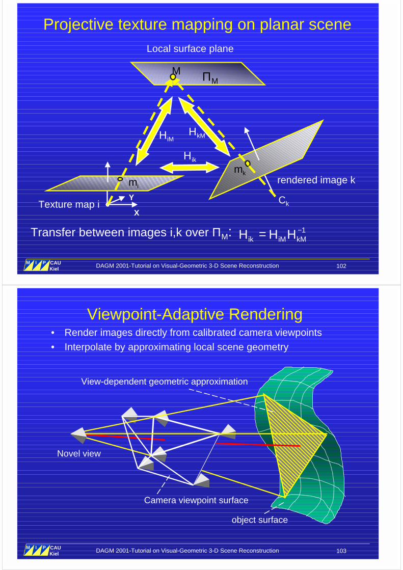
Projective texture mapping on planar scene

X

YTexture map i

im

M

km

Ck

ΠM

iMH

ikH

kMH

1ik iM kMH H H −=Transfer between images i,k over ΠM:

rendered image k

Local surface plane



CAUKiel

Viewpoint-Adaptive Rendering• Render images directly from calibrated camera viewpoints• Interpolate by approximating local scene geometry


object surface


Novel view



CAUKiel

Viewpoint-Adaptive Rendering


object surface


Novel view

• Render images directly from calibrated camera viewpoints• Interpolate by approximating local scene geometry• Scalable geometrical approximation through subdivision

Rendering: 3 projective mappings and α-blending per triangle (OpenGL Hardware)



CAUKiel

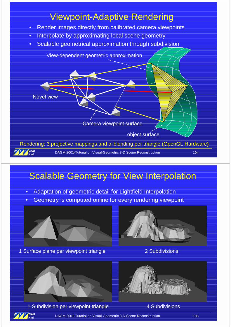
Scalable Geometry for View Interpolation

1 Surface plane per viewpoint triangle

4 Subdivisions

2 Subdivisions

1 Subdivision per viewpoint triangle

• Adaptation of geometric detail for Lightfield Interpolation• Geometry is computed online for every rendering viewpoint



CAUKiel

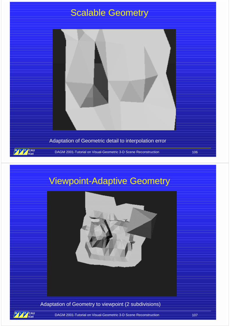
Scalable Geometry

Adaptation of Geometric detail to interpolation error



CAUKiel

Viewpoint-Adaptive Geometry

Adaptation of Geometry to viewpoint (2 subdivisions)



CAUKiel

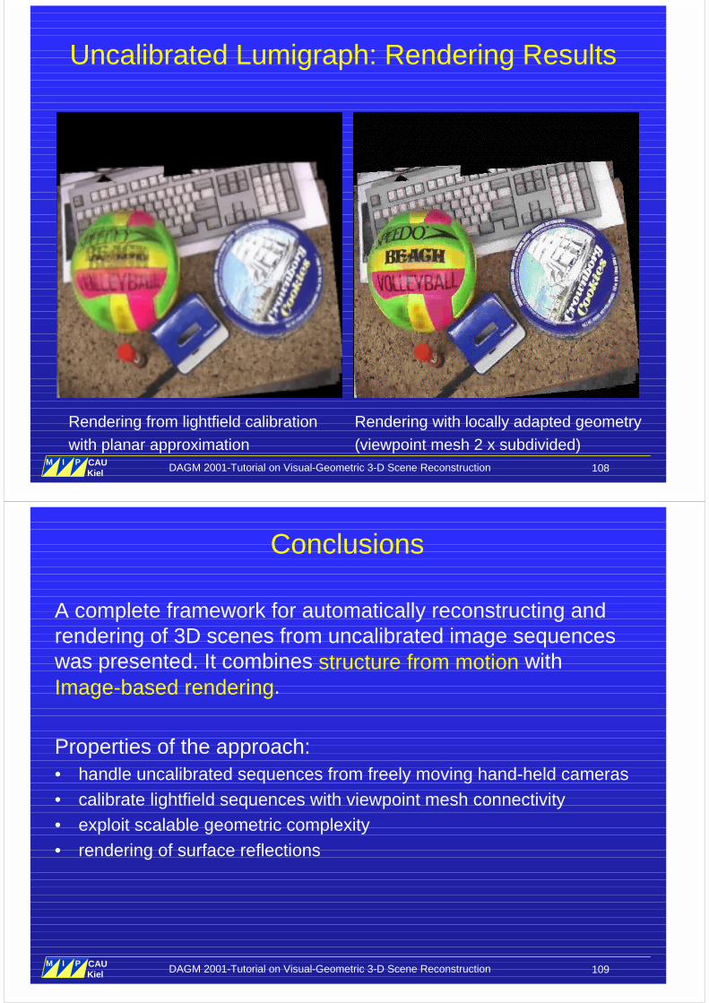
Uncalibrated Lumigraph: Rendering Results

Rendering from lightfield calibrationwith planar approximation

Rendering with locally adapted geometry(viewpoint mesh 2 x subdivided)



CAUKiel

Conclusions

A complete framework for automatically reconstructing andrendering of 3D scenes from uncalibrated image sequenceswas presented. It combines structure from motion withImage-based rendering.

Properties of the approach:• handle uncalibrated sequences from freely moving hand-held cameras• calibrate lightfield sequences with viewpoint mesh connectivity• exploit scalable geometric complexity• rendering of surface reflections

Documents

MI P Visual-Geometric Multimedia Information … · 3-D Scene Reconstruction from Uncalibrated Image Sequences ... Multimedia Information Processing ... 3. 3-D scene reconstruction