MHF4U Unit 1 - Ontario€¢ BLM 1.1.1, 1.1.2 Assessment ... the progress of students who had ... TIPS4RM: MHF4U: Unit 1 – Polynomial Functions 2008 8

TIPS4RM: MHF4U: Unit 1 – Polynomial Functions 2008 1

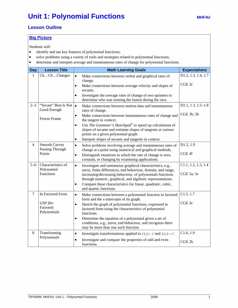
Unit 1: Polynomial Functions MHF4U Lesson Outline Big Picture Students will: • identify and use key features of polynomial functions; • solve problems using a variety of tools and strategies related to polynomial functions; • determine and interpret average and instantaneous rates of change for polynomial functions.

Day Lesson Title Math Learning Goals Expectations 1 Ch…Ch…Changes • Make connections between verbal and graphical rates of

change. • Make connections between average velocity and slopes of

secants. • Investigate the average rates of change of two sprinters to

determine who was running the fastest during the race.

D1.2, 1.3, 1.4, 1.7 CGE 3c

2–3 “Secant” Best Is Not Good Enough Freeze Frame

• Make connections between motion data and instantaneous rates of change.

• Make connections between instantaneous rates of change and the tangent in context.

• Use The Geometer’s Sketchpad® to speed up calculations of slopes of secants and estimate slopes of tangents at various points on a given polynomial graph.

• Interpret slopes of secants and tangents in context.

D1.1, 1.3, 1.5–1.8 CGE 3b, 5b

4 Smooth Curves Passing Through Points

• Solve problems involving average and instantaneous rates of change at a point using numerical and graphical methods.

• Distinguish situations in which the rate of change is zero, constant, or changing by examining applications.

D1.2, 1.9 CGE 4f

5–6 Characteristics of Polynomial Functions

• Investigate and summarize graphical characteristics, e.g., zeros, finite differences, end behaviour, domain, and range, increasing/decreasing behaviour, of polynomials functions through numeric, graphical, and algebraic representations.

• Compare these characteristics for linear, quadratic, cubic, and quartic functions.

C1.1, 1.2, 1.3, 1.4 CGE 5a, 5e

7 In Factored Form GSP file: Factored Polynomials

• Make connections between a polynomial function in factored form and the x-intercepts of its graph.

• Sketch the graph of polynomial functions, expressed in factored form using the characteristics of polynomial functions.

• Determine the equation of a polynomial given a set of conditions, e.g., zeros, end behaviour, and recognize there may be more than one such function.

C1.5, 1.7 CGE 3c

8 Transforming Polynomials

• Investigate transformations applied to ( ) 3f x x= and ( ) 4.f x x= • Investigate and compare the properties of odd and even

functions.

C1.6, 1.9 CGE 2b


Day Lesson Title Math Learning Goals Expectations 9–10

(lessons not included)

• Divide polynomials. • Examine remainders of polynomial division and connect to

the remainder theorem. • Make connections between the polynomial function ( ),f x the

divisor ,x a− the remainder of the division ( )( )

f xx a−

and ( )f a

using technology. • Identify the factor theorem as a special case of the remainder

theorem. • Factor polynomial expressions in one variable of degree no

higher than four.

C3.1, 3.2

11–12


• Solve problems graphically and algebraically using the remainder and factor theorems.

• Solve polynomial equations by selecting an appropriate strategy, and verify with technology.

• Make connections between the x-intercepts of a polynomial function and the real roots of the corresponding equation.

• Use properties of polynomials to fit a polynomial function to a graph or a given set of conditions.

• Determine the equation of a particular member of a family of polynomials given a set of conditions, e.g., zeros, end behaviour, point on the graph [See Home Activity and graphs for Day 7.]

C1.8, 3.3, 3.4, 3.7

13–14


• Understand the difference between the solution to an equation and the solution to an inequality.

• Solve polynomial inequalities and simple rational inequalities by graphing with technology.

• Solve linear inequalities and factorable polynomial inequalities.

• Represent the solution to inequalities on a number line or algebraically.

C4.1, 4.2, 4.3

15–16

Jazz Days

17 Summative Assessment


Unit 1: Day 1: Ch… Ch… Changes MHF4U

75 min

Math Learning Goals • Make connections between verbal and graphical rates of change. • Make connections between the average velocity and slope of the secant line. • Investigate the average rates of change of two sprinters to determine who was

running the fastest during the race.

Materials • BLM 1.1.1, 1.1.2

Assessment Opportunities

Minds On… Think/Pair/Share Matching Activity Students categorize the rates of change of the graphs as either: zero, constant, or changing (BLM 1.1.1). Ask: • Which graphs have a rate of change of zero? How do you know? • Which graphs have a constant rate of change? How can you tell? • Which graphs have a non-constant rate of changing? How do you know?

Students match verbal and graphical rates of change (BLM 1.1.1).

Mathematical Process/Connecting/Observation/Mental Note: Conduct a poll to determine correctness of pairs’ matches to graph A, e.g., using clickers or TI-Navigator or by holding up a sheet with the number written on it. Ask a pair with the correct answer to explain their strategy.

Use an overhead of BLM 1.1.1 to match graph A to its description. Use the same coloured marker to connect the words, the features of the graph and student strategies. Ask: Did any pair use a different strategy? Pairs discuss their strategies and matches for the remaining graphs (B–E). Poll answers to the remaining questions on the overhead. Highlight that the independent variable for each graph is time. For each graph students identify the missing dependent variable.

Action! Whole Class Teacher-Directed Instruction

Provide students with the definition of average rate of change as yx

ΔΔ

and

connect to their experiences with slope; then specifically to the average velocity

as averagedVt

Δ=Δ

Pairs Investigation Pairs complete Part A of BLM 1.1.2.

Curriculum Expectations/Observation/Mental Note: Circulate to ensure that pairs are getting correct answers. Make a mental note to consolidate misconceptions.

Consolidate Debrief

Whole Class Sharing Students with correct understanding of concepts misunderstood by their classmates explain their responses. Students should have connected the relationship between the average rate of change and the slope of the secant.

Circulate to monitor the progress of students who had incorrect answers. Word Wall • dependent variable • independent

variable • velocity • average rate of

change

• y

x

Δ

Δ

• secant

Exploration Application

Home Activity or Further Classroom Consolidation Complete Parts B and C of Worksheet 1.1.2.


1.1.1: Ch… Ch… Changes • Circle the rate of change as zero, constant, or changing for each graph. • Match the graphs with the descriptions given on the right. • Be prepared to explain your reasoning.

Graphs Description A

Rate of Change: zero constant changing

1. A Grade 12 student's height over the next 12 months.

B


2. Money deposited on your 12th birthday grew slowly at first, then more quickly.

C


3. Andrea walks quickly, slows to a stop, and then speeds up until she is travelling at the same speed as when she started.

D


4. Over a one-month period the rate of growth for a sunflower is constant.

E


5. Clara walks quickly and then slows to a stop. She then walks quickly and slows to a second stop. Clara then walks at a pace that is a little slower than when she started.


1.1.2: A Race to the Finish Line During the 1997 World Championships in Athens, Greece, Maurice Greene and Donovan Bailey ran a 100 m race. (http://hypertextbook.com/facts/2000/KatarzynaJanuszkiewicz.shtml) Part A The graph and table below show Donovan Bailey’s performance during this 100 m race.

Donovan Bailey’s Performance

Time (s) Distance (m) .000 00. 1.78 10. 2.81 20. 3.72 30. 4.59 40. 5.44 50. 6.29 60. 7.14 70. 8.00 80. 8.87 90. 9.77 100.

1. a) Calculate Donovan Bailey’s average velocity for this 100 m sprint.

change in distanceAverage Velocitychange in time

dt

Δ= =

Δ

b) Draw a line from ( ),0 0 to ( ). ,9 77 100 on the graph above.

A line passing through at least two different points on a curve is called a secant. c) Explain the relationship between your answer to a) and the slope of the secant.

2. a) Draw the secants from ( ),0 0 to ( ). ,5 44 50 and from ( ). ,5 44 50 to ( ). ,9 77 100 .

b) Calculate the average velocities represented by the two secants drawn in a).

i) ii)


1.1.2: A Race to the Finish Line (continued) 2. c) Compare Bailey’s performance during the first and the second half of the race. 3. Describe the relationship between average velocity and the slope of the corresponding

secant. 4. Calculate Bailey’s average velocity for each 10 m interval of this 100 m race. Record your

answers in the table below.

Interval (m)

Distance Travelled Δd (m)

Time Elapsed Δt (s)

Average Velocity (m/s)

0 to 10

10 to 20

20 to 30

30 to 40

40 to 50

50 to 60

60 to 70

70 to 80

80 to 90

90 to 100


1.1.2: A Race to the Finish Line (continued) Part B The graph and table show Maurice Greene’s performance during the same 100 m race.

Maurice Greene’s Performance

Time (s) Distance (m) 0 0 1.71 10 2.75 20 3.67 30 4.55 40 5.42 50 6.27 60 7.12 70 7.98 80 8.85 90 9.73 100

Calculate Greene’s average velocity for each 10 m interval of this 100 m race. Record your answers in the table below.

Interval (m)

Distance Travelled Δd (m)

Time Elapsed Δt (s)

Average Velocity (m/s)

0 to 10

10 to 20

20 to 30

30 to 40

40 to 50

50 to 60

60 to 70

70 to 80

80 to 90

90 to 100 Part C Using your calculations from Parts A and B, describe this 100 m race run by Donovan Bailey and Maurice Greene. Include who was fastest and who was leading at various points during the race.


Unit 1: Day 2: “Secant” Best Is Not Good Enough MHF4U

75 min

Math Learning Goals • Make connections between collected motion data to instantaneous rates of change. • Make connections between average and instantaneous rates of change as they relate

to other real world applications.

Materials • BLM 1.2.1, 1.2.2,

1.2.3 • graphing

calculators • CBRs


Minds On… Small Groups Exploration Students generate the graphs of linear, quadratic, and cubic functions using the CBR and graphing calculators (BLM 1.2.1).

Whole Group Discussion Discuss strategies students used to replicate the graphs referring to connections between the motion and the average rates of change.

Action! Small Groups Investigation Students use a CBR to gather distance vs. time data with the goal of having the fastest rate of change at t = 1 s (BLM 1.2.2).

Learning Skills/Collaborate and Teamwork/Observation/Checklist: Observe students’ ability to work collaboratively.

Consolidate Debrief

Whole Class Debrief Ask 2 or 3 groups who finish first to prepare to share their data with the class, either on the board, overhead projector, SMART Board™, document camera or chart paper. Ask the group who ran the fastest to prepare to display their graphs including the secant lines. While examining the numerical data, ask the class: • How did the average velocities help you to estimate the velocity at 1s? • How accurate were the estimations? • What contributed to the accuracy?

Class discussion should include the calculation of average velocities over smaller intervals and how average velocities are used to approximate instantaneous velocities. Make connections between the numerical and graphical data: Use a straight edge to trace the secant lines for the displayed graph. Make connections between the slope of the secant lines and the average velocities: On their graphs students name this line the tangent as representing the velocity at t = 1.

Students may have to walk the line several times to match graphs. Check to ensure students are smoothing their graphs rather than connecting using line segments. Word Wall • instantaneous rate

of change • tangent

Application Exploration Reflection

Home Activity or Further Classroom Consolidation Complete Instantaneous Success (Worksheet 1.2.3). Write a journal entry that summarizes your new learning about: secants, tangents, average rates of change, and instantaneous rates of change.


1.2.1: Race Match Challenge In this activity you will be walking three different walks. The first walk will model a linear function, the second will model a quadratic function, and the third will model a cubic function. Instructions 1. Attach the CBR to your graphing calculator. 2. Press APPS and select CBL/CBR by pressing ENTER. 3. Press any key to enter the CBL/CBR program. 4. Select 3: RANGER and press ENTER to continue. 5. Select 1: SETUP/SAMPLE 6. Bring the arrow (cursor) to the START NOW option and press ENTER. 7. When you are ready press ENTER to start collecting data. Walk 1 – Linear Walk Place yourself 3 metres from the CBR and walk towards the CBR at a constant velocity until you are 0.5 metres away. Your graph should look like the graph below. Draw a sketch of your walk on the second graph below. Is the average velocity constant? If not, over what interval were you travelling the fastest?

Walk 2 – Quadratic Walk Walk towards the CBR and gradually reduce your walking rate (velocity) until you are 0.5 metres from the CBR then walk away from the CBR gradually increasing your velocity. Your graph should look like the graph below. Draw a sketch of your walk on the second graph below. Is the average velocity constant? If not, over what interval were you travelling the fastest?

Walk 3 – Cubic Walk Place yourself 3 metres away from the CBR. Create a walk similar to the one below. Draw a sketch of your walk on the second graph below. Is the average velocity constant? If not, over what interval were you travelling the fastest?


1.2.2: “Secant” Best Is Not Good Enough You are to determine the fastest student at the 1 second point of the race. Stand 0.5 metres away from the CBR. With your partner, plan your motion so that you will be moving as fast as possible 1 second after the CBR has started. Using your knowledge of average rates of change, determine the fastest person in the class at t = 1 s. 1. Attach the CBR to your graphing calculator. 2. Press APPS and select CBL/CBR by pressing ENTER. 3. Press any key to enter the CBL/CBR program. 4. Select 3: RANGER and press ENTER to continue. 5. Select 1: SETUP/SAMPLE 6. Bring the arrow (cursor) to the START NOW option and press ENTER. 7. Have your partner stand 0.5 m away from the CBR. When you are ready press ENTER to

start collecting data and have your partner run away from the CBR. 8. Draw a sketch of your graph below.

9. Using the cursor keys find two points that you can use to determine the average velocity for

the first 2 seconds. Draw a secant on the graph above to represent this average velocity. 10. Use the cursor keys to fill in the following table:

t (s) 0 0.5 0.9 1 1.1 1.5 2

d(m)

11. a) Calculate the average velocity over the following intervals.

0–1 s 0.5–1 s 0.9–1 s 1–1.1 s 1–1.5 s 1–2 s

b) Using these calculations, estimate the velocity at t = 1 s. Does your answer from a)

accurately represent the velocity at t = 1 s? Explain. c) How could you improve the estimate from b)?


1.2.2: “Secant” Best Is Not Good Enough (continued) 12. a) Use the data points from Question 10 to construct a more accurate graph below.

b) Sketch the secant lines that represent the average velocities over each interval found in Question 11.

c) How does the slope of the secant lines connect to the average velocities? d) Sketch the graph of the line to represent the estimated velocity at t = 1 s.


1.2.3: “Instant”aneous Success! In 1997, Donavan Bailey ran the 100 m sprint in 9.77 seconds. The table below describes his run. One model that describes this run is a quadratic model with an equation of: ( ) . . .20 28 8 0 2 54s t t t= + − .

Time (s)

Distance (m)

0.00 0. 1.78 10. 2.81 20. 3.72 30. 4.59 40. 5.44 50. 6.29 60. 7.14 70. 8.00 80. 8.87 90. 9.77 100.

1. a) Estimate Donavan Bailey’s instantaneous velocity at t = 6 s.

b) Explain why your answer to a) is a good approximation.

c) Plot a point on the curve at 6 seconds. Draw a line that passes through this point but does not pass through the curve again. This line is called a tangent to the curve.


1.2.3: “Instant”aneous Success! (continued) 2. Either by hand or with technology, use the algebraic model ( ) . . .20 28 8 02 2 54s t t t= + − to

approximate the instantaneous velocity of Donavan Bailey at t = 6 s.

a) Reset your graphing calculator b) Enter the equation of Bailey’s run by pressing Y= c) Set the Window using the axes above as a guide. d) Press Graph. e) Press Trace and then 6 Enter to position the cursor at t = 6 s, record the y-value. f) Press Trace and 7 Enter, record the y-value. g) Calculate the average velocity over this interval.

Point A Point B Average Velocity

x-value 6 x-value 7 y-value y-value

h) Repeat steps f) and g) above two more times, each time choosing a point closer to t = 6 s. Calculate the average velocities over these intervals.

Point A Point B Average Velocity x-value 6 x-value y-value y-value

Point A Point B Average Velocity

x-value 6 x-value y-value y-value

i) Use the calculations from steps g) and h) to estimate the instantaneous velocity at t = 6 s.

j) Draw the secants (on the graph) that correspond with the three average velocities calculated above. How do the secants compare to the tangent drawn in 1(c)?


Unit 1: Day 3: Freeze Frame MHF4U

75 min

Math Learning Goals • Make connections between the instantaneous rate of change and the tangent in a

real world context. • Use The Geometer’s Sketchpad® to speed up calculations of slopes of secants and

estimate slopes of tangents at various points on a given polynomial graph. • Interpret slopes of secants and tangents in contexts.


1.3.3 • The Geometer’s

Sketchpad®


Minds On… Small Groups Sorting Activity To make sense of their relationships, students sort descriptions into 3 sets – those describing average rates of change, those that are close to instantaneous rates of change, and those that are instantaneous rates of change (BLM 1.3.1).

Mathematical Process/Connecting/Observation/Mental Note: Listen to group discussions to determine students’ ability to determine the rate of change type.

Whole Class Discussion Guide a class discussion focused on misconceptions and different points of view observed in small group activity. Challenge each group to create one unique example of average rate of change, close to average rate of change, and instantaneous rate of change.

Action! Pairs Investigation Pairs complete the investigation using The Geometers’ Sketchpad® (BLM 1.3.2). Pairs work on completing the questions, keeping their own notes.

Consolidate Debrief

Whole Class Reflection Guide student reflection on the use of technology to determine the instantaneous rate of change from the activity. Given a function, discuss strategies for determining the instantaneous rate of change without technology. Highlight responses that focus on finding the slope over a very small interval.

Measurements, although described as instantaneous, are based on a small interval of time, and should be referred to as close to instantaneous. BLM 1.3.1 Answers: Average – 1, 3, 5, 7 Close to – 2, 4, 8 Instant – 6

Reflection

Home Activity or Further Classroom Consolidation Complete Worksheet 1.3.3 by hand or using technology.

Student licensed take-home version of GSP® is available through the IT department at boards.


1.3.1: Average, Close to Instant, or Instant?

1. Some road tolls in the U.S. give speeding tickets based on the time it takes you to travel between exits.

2. A police officer pulls you over for speeding since her radar gun displays 130 km/hr.

3. Canada’s population grew at a rate of 0.869% from 2006 to 2007.

4. Roy Halliday’s fast ball was measured to have a velocity of 152 km/h.

5. Your parents kept a growth chart from the time you were 1 until you were 5 years old. They have calculated that your growth rate in that period was 9 cm/year.

6. In 1996, Hurricane Bertha had wind gusts up to185 km/h. At some times during Hurricane Bertha the wind was gusting at 100 km/h.

7. Water is being poured into a container. The rate in which the water level increases between 0 and 5 seconds of the pour is 7 mm/sec.

8. A CO2 probe measures the rate of increase of atmospheric CO2. The probe reads an increase of 1.7 × 10–8 ppm/sec.


1.3.2: Sketching a Sprinter’s Path 1. Open The Geometer’s Sketchpad®. 2. From the menu bar select Graph Plot New Function. 3. Enter the equation given yesterday of Bailey’s sprint, ( ) . . . ,s t t t= + −20 28 8 0 2 54 then press

OK. (Note: Replace t with x.)

4. From the menu bar select Graph Rectangular Grid. 5. Change the y-scale of the graph to show a range that includes 0 to 100 m by clicking the red

dot on the axis and dragging it down.

6. Select the graph of the function and from the menu bar select Construct Point On

Function Plot. 7. Deselect all objects by clicking on a blank part of the grid. 8. Repeat step 6 to create another point on the curve.

9. Using the labelling tool , label one point A and the other point B. 10. Select point A and from the main menu select Measure Abscissa (x). This value

represents the x-value (time) of point A. 11. Repeat step 10 using point B. 12. Select both points on the curve and select Construct Line from the main menu. 13. Select the line and from the menu bar select Measure Slope. This represents the

slope of the secant. 14. Find the slope between the x-values 6 and 7.


1.3.2: Sketching a Sprinter’s Path (continued) 15. Compare the slope from Question 14 to the average velocity between 6 and 7 seconds and

the velocity of Donovan Bailey’s run. What do you notice? 16. How is the slope of the secant related to the average velocity? 17. Find the average velocity by dragging both points of Donavan Bailey’s run for the intervals

given in the table below:

Interval Average Velocity (m/s) Between 0.5 and 2 seconds Between 0.5 and 1.5 seconds Between 0.5 and 1 seconds Between 0.5 and 0.6 seconds

18. Describe a method for determining Bailey’s instantaneous velocity at time t. 19. Donavan Bailey’s instantaneous velocity was measured during the race at different time

values as shown in the table below. Verify if these values are correct using the points you created on the function.

Time (s)

Actual Instantaneous Velocity

(m/s)

Calculated Instantaneous Velocity

(m/s) 1.78 8.90 2.81 10.55 3.72 11.28 4.59 11.63 5.44 11.76 6.29 11.80 7.14 11.70 8.00 11.55 8.87 11.38 9.77 11.00

20. Does your calculated data match the actual data? Explain why or why not.


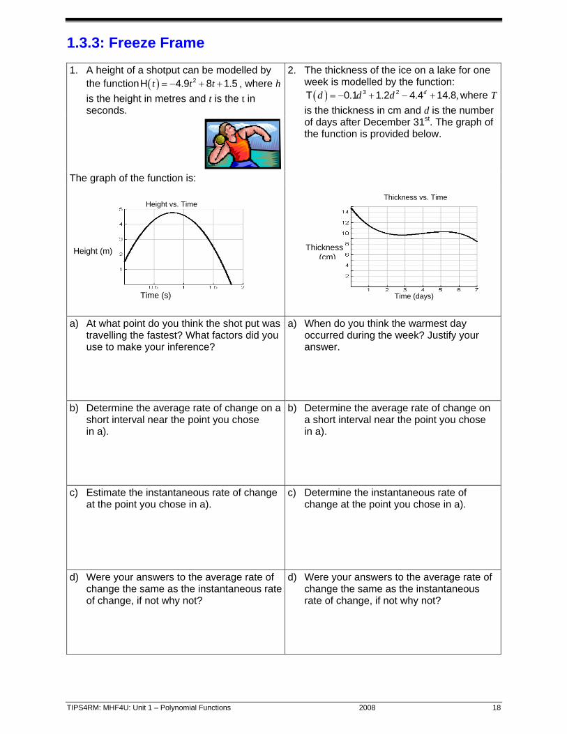
1.3.3: Freeze Frame 1. A height of a shotput can be modelled by

the function ( ) . .2H 4 9 8 1 5t t t= − + + , where h is the height in metres and t is the t in seconds.

The graph of the function is:

2. The thickness of the ice on a lake for one week is modelled by the function: ( ) . . . . ,dd d d= − + − +3 2T 0 1 1 2 4 4 14 8 where T

is the thickness in cm and d is the number of days after December 31st. The graph of the function is provided below.

a) At what point do you think the shot put was travelling the fastest? What factors did you use to make your inference?

a) When do you think the warmest day occurred during the week? Justify your answer.

b) Determine the average rate of change on a short interval near the point you chose in a).

b) Determine the average rate of change on a short interval near the point you chose in a).

c) Estimate the instantaneous rate of change at the point you chose in a).

c) Determine the instantaneous rate of change at the point you chose in a).

d) Were your answers to the average rate of change the same as the instantaneous rate of change, if not why not?

d) Were your answers to the average rate of change the same as the instantaneous rate of change, if not why not?

Time (s)

Height (m)

Height vs. Time

Time (days)

Thickness (cm)

Thickness vs. Time


Unit 1: Day 4: Smooth Curves Passing Through Points MHF4U

75 min

Math Learning Goals • Solve problems involving average and instantaneous rates of change at a point

using numerical and graphical methods. • Distinguish situations in which the rate of change is zero, constant, or changing by

examining applications.

Materials • BLM 1.4.1


Minds On… Pairs Discussion Students compare their solutions in pairs (BLM 1.3.3).

Curriculum Expectations/Observation/Mental Note: Circulate to determine that pairs are getting correct answers, and team up pairs as necessary to undo misconceptions.

Groups of 4 Place Mat Students create a place mat with four divisions and a circle in the centre. Individually students write their description of the instantaneous rate of change of a function at a point in their section of the place mat. Group consensus is written in the centre of their place mat. One member of each group shares their statement(s) with the whole class. Discuss as a class common points and any misconceptions about instantaneous rates of change. Groups make changes to their description as needed.

Curriculum Expectations/Observation/Mental Note: Listen to groups’ descriptions of rate of change to form ability groupings for Action! section.

Action! Groups of 4 Investigation Form homogeneous groups based on observations during Minds On… activity – students with a thorough understanding work on Graph B of BLM 1.4.1; others work on Graph A. Inform students that the context for graphs comes from BLM 1.3.3. Select a group that worked on Graph A to share responses from their investigation for Question 1 and a group to share responses from Graph B. Students copy the information for the graphs they did not work on to complete the remaining questions.

Consolidate Debrief

Whole Class Sharing Discuss the remaining questions. Highlight similarities between the signs of the slopes of the tangents between the two graphs. Select two students to trace the curves with a straight edge to demonstrate the trend in the slopes of the tangents as time changes – bring out connections to the key characteristics of graphs (intervals of increase/decrease, local maximum/minimum).

Think Literacy: Literacy Strategy: Place mat

Journal Entry

Home Activity or Further Classroom Consolidation Enter what you know about rates of changes and key characteristics of graphs in your journal.

Think Literacy Strategy: Journals


Thickness (cm)

Time (days)

Thickness vs. Time

1.4.1: Tangent Slopes and Graph Characteristics 1. Using the graphs below determine the instantaneous rates of change ( )Tm for one of the

graphs at the given points. A.

B.

t 0 0.25 0.5 0.8 1 1.5 1.8 t 0 1 2 3 4 5 6 7

Tm Tm 2. State the domain and the range of the two functions.

Graph A Graph B: Domain: Domain: Range: Range:

3 a) Describe the graphical feature, e.g., local maximum/minimum point, interval of

increase/decrease, Tm values (e.g., +, –, 0), and, where appropriate, the trend of the slope of the tangent, e.g., changing from positive to zero to negative, as time increases.

Interval Graphical feature Tm values Tm trend

(if appropriate) Graph A: Domain 0-0.8 Graph A: at 0.8 Graph A: Domain 0.8–1.75 Graph B: Domain 0–3 Graph B: at 3 Graph B: Domain 3–5 Graph B: at 5 Graph B: Domain 5–7

b) Describe the context where the slope of the tangent is zero. What does it mean? c) What are the similarities and differences between the slopes of the tangents?

Time (s)

Height (m)

Height vs. Time


1.4.1: Tangent Slopes and Graph Characteristics (continued) 4. The slope of a secant line can be a good estimate of the slope of the tangent. Rod thought

that using an interval of 1 second to determine the slope of the secant line in Graph A is good enough to use to determine the slope of the tangent. Do you agree or disagree? Justify your reasoning.

5. For Graph A, state the slope of the tangent at 0.5 and 1 second. At which point is the shot

put going faster? Explain. 6. Draw three or four curves that have a secant slope of 2 and that pass through the same two

points. What inference can be made from this? 7. Anne says that a tangent crosses a curve in one and only one point. Do you agree or

disagree? Use Graph B to justify your position.


Unit 1: Day 5: Characteristics of Polynomial Functions MHF4U

75 min

Math Learning Goals • Investigate and summarize the graphical characteristics, e.g., zeros, finite

differences, end behaviour, domain and range, increasing/decreasing behaviour, of polynomial functions given algebraic, expanded form, and numeric representations.


1.5.3 • graphing

calculator


Minds On… Think/Pair/Share Concept Attainment Activity Students compare the data sets and answer questions on BLM 1.5.1 to distinguish between mathematical relationships that are and are not polynomial functions. During whole class sharing, guide development of a class summary of polynomial functions for the Word Wall, e.g., using a Frayer model with quadrant headings: definition, facts, examples, non-examples.

Action! Small Groups or Pairs Investigation Students use GSP® files – Quartic Polynomial Investigation, Cubic Polynomial Investigation, and Linear and Quadratic Polynomial Investigation – to manipulate sliders on parameters in the equations. Alternatively, students use graphing calculators to explore the graphical effects of changing a, b, c, d, and k parameters in equations ,y ax k= + 2 ,y ax bx k= + +

3 2 ,y ax bx cx k= + + + and 4 3 2 .y ax bx cx dx k= + + + + Students summarize some of the graphical characteristics (e.g., overall shape, end behaviour, domain and range, increasing/decreasing behaviour, maximum number of zeros; single, double, and triple roots of the corresponding equations) without yet making precise links between the algebraic conditions leading to these various types of roots (BLM 1.5.2).

Learning Skills (Initiative)/Observation/Rating Scale: Observe how the students individually demonstrate initiative as they conduct their group investigations.

Whole Class Presentations Different groups use the GSP® files and a SMART Board™ to demonstrate the properties of quartic, cubic, quadratic, and linear polynomial functions, and capture summaries in a SMART Notebook™ file for class sharing. Alternatively, groups use large chart paper to record their responses.

Consolidate Debrief

Whole Class Presentations Students individually hypothesize the answers to questions such as the following: • What is the effect of changing the degree of the polynomials? • What is the effect of the leading coefficient being positive or negative? • What is the maximum number of x-intercepts for given a function and how do

you know?

Record all hypotheses. Guide a discussion as to how the hypotheses could be tested. Model the testing of the hypotheses using the GSP® file and/or the artefacts of the whole class presentations.

Sample Definition: A polynomial function is a relationship whose equation can be expressed in the form y = (an expression that is constructed from one or more variables and constants, using only the operations of +, -, ×, and constant positive whole number exponents). For each x-value in the domain, there corresponds one and only one element in the range. Sample Facts: • Exponents on x are

whole numbers • No variables in

denominators • Graphs are smooth

continuous curves You may wish to address these questions one at a time.

Concept Practice Home Activity or Further Classroom Consolidation Complete Worksheet 1.5.3.


1.5.1: Polynomial Concept Attainment Activity Compare and contrast the examples and non-examples of polynomial functions below. Through reasoning, identify 3 attributes of every polynomial function that distinguish them from non-polynomial functions:

a. _______________________________________

b. _______________________________________

c. _______________________________________

Examples Non Examples

y x= y x=

2 1y x= − ( )123f x x x= −

25

y x= − 6x = −

2y x= 2 2 16x y+ =

( )22 1y x= − + ( ) 3h x x=

( ) 2f x x x= − + y β= sin

( )( ).0 2 4 3 3y x x= − − + 12

yx

=−

3 22 11y x x x= + − + 2xy =


1.5.1: Polynomial Concept Attainment Activity (continued)

Examples Non Examples

4y = 2

11

xyx x

−=

− +

( ) 4 21 32

h x x x= − + −

( )( )

0

2

4 4

4 2

y x

y x x x

= − +

= − +


1.5.2: Graphical Properties of Polynomial Functions 1. Use technology to graph a large number of polynomial functions y = ax + k that illustrate

changes in a, b, c, d, and k values. Certain patterns will emerge as you try different numerical values for a, b, c, d, and k. Remember that any of b, c, d, and k can have a value of 0. Your goal is to see patterns in overall shapes of linear, quadratic, cubic, and quartic polynomial functions, and to work with properties of the functions, rather than to precisely connect the equations and graphs of the functions – the focus of later work. Answer the questions by referring to the graphs drawn using technology.

2

0y ax bx ka= + +≠

3 2

0y ax bx cx ka= + + +≠

4 3 2

0y ax bx cx dx ka= + + + +≠

Instructions Linear Quadratic Cubic Quartic

Sketch, without axes, the standard curve (i.e., a = 1, and b, c, d, and k all = 0), and state the equation of the curve

No zeros No zeros Why is it impossible to have no zeros?

No zeros

Just 1 zero Just 1 zero Just 1 zero (Hint: 2 shapes possible)

Just 1 zero

Exactly 2 zeros Exactly 2 zeros Exactly 2 zeros (Hint: 2 axes placements possible)

Exactly 3 zeros Exactly 3 zeros

Sketch the basic shape, then place the x- and y-axes to illustrate the indicated numbers of zeros. Enter a sample equation for each sketch

Explain why there can be no more than 1 zeros

Explain why there can be no more than 2 zeros

Exactly 4 zeros


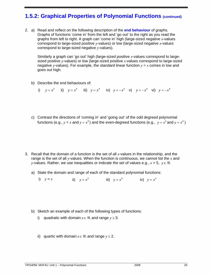
1.5.2: Graphical Properties of Polynomial Functions (continued) 2. a) Read and reflect on the following description of the end behaviour of graphs.

Graphs of functions ‘come in’ from the left and ‘go out’ to the right as you read the graphs from left to right. A graph can ‘come in’ high (large-sized negative x-values correspond to large-sized positive y-values) or low (large-sized negative x-values correspond to large-sized negative y-values).

Similarly a graph can ‘go out’ high (large-sized positive x-values correspond to large-sized positive y-values) or low (large-sized positive x-values correspond to large-sized negative y-values). For example, the standard linear function y = x comes in low and goes out high.

b) Describe the end behaviours of:

i) 2y x= ii) 3y x= iii) 4y x= iv) 2y x= − v) 3y x= − vi) 4y x= −

c) Contrast the directions of ‘coming in’ and ‘going out’ of the odd degreed polynomial functions (e.g., y = x and 3y x= ) and the even-degreed functions (e.g., 2y x= and 4y x= )

3. Recall that the domain of a function is the set of all x-values in the relationship, and the

range is the set of all y-values. When the function is continuous, we cannot list the x and y-values. Rather, we use inequalities or indicate the set of values e.g., x > 5, y∈ℜ. a) State the domain and range of each of the standard polynomial functions:

i) y = x ii) 2y x= iii) 3y x= iv) 4y x=

b) Sketch an example of each of the following types of functions:

i) quadratic with domain x∈ℜ. and range .3y ≥

ii) quartic with domain x∈ℜ. and range 2y ≤ .


1.5.2: Graphical Properties of Polynomial Functions (continued) 4. Recall that a function is increasing if it rises upward as scanned from the left to the right.

Similarly, a function is decreasing if it goes downward as scanned from the left to the right. A function can have intervals of increase as well as intervals of decrease. For example, the standard quartic function 4y x= decreases to x = 0, then increases.

a) Sketch a cubic function that increases to x = –3, then decreases to x = 4, then increases. b) Use graphing technology to graph ,4 25 4y x x= − + sketch the graph, then describe the

increasing and decreasing intervals. 5. Compare and contrast the following pairs of graphs:

a) y = x and y = –x b) 2y x= and 2y x= −

c) 3y x= and 3y x= − d) 4y x= and 4y x= −


1.5.3: Numerical Properties of Polynomial Functions

x y First Differences

–3

–2

–1

0

1

2

1. Consider the function y = x a) What type of function is it? b) Complete the table of values. c) Calculate the first differences. d) In this case, the first differences

were positive. How would the graph differ if the first differences were negative?

3

Differences x y First Second

–3

–2

–1

0

1

2

2. Consider the function 2y x= a) What type of function is it? b) Complete the table of values. c) Calculate the first and second

differences.

3


1.5.3: Numerical Properties of Polynomial Functions (continued)

Differences x y First Second Third

–3

–2

–1

0

1

2

3. Consider the function 3y x= a) What type of function is it? b) Complete the table of values. c) Calculate the first, second,

and third differences.

3

Differences x y First Second Third Fourth

–3 –2

–1

0

1 2

4. Consider the function y x= 4 a) What type of

function is it? b) Complete the

table of values. c) Calculate the

first, second, third, and fourth differences.

3

5. a) Summarize the patterns you observe in Questions 1–4.

b) Hypothesize as to whether or not your patterns hold when values for the b, c, d, and k parameters are not equal to 0 in ,y ax k= + ,2y ax bc k= + + ,3 2y ax bx cx k= + + + and

.4 3 2y ax bx cx dx k= + + + +

c) Test your hypothesis on at least 6 different examples. Explain your findings.


Unit 1: Day 6: Characteristics of Polynomial Functions MHF4U

75 min

Math Learning Goals • Investigate and summarize the graphical characteristics, e.g., finite differences,

domain and range, increasing/decreasing behaviour, local and overall maximums and minimums, of polynomial functions given algebraic, expanded form, and numeric representations.

• Compare these characteristics for linear, quadratic, cubic and quartic functions.

Materials • BLM 1.6.1 • graphing

calculators


Minds On… Groups of Three Card Game Randomly hand each student a card (BLM 1.6.1). Students search for the algebraic, graphical, and numerical forms of their function. Each group gathers together to record and display its set of 3 representations for the same function. Each group: • records the domain and range • colours increasing intervals of the function blue • colours decreasing intervals of the function pink

Action! Whole Class Developing Academic Language Point to a local maximum on one of the displayed graphs, and ask students to consider whether that point should be coloured pink or blue. Guide the discussion that an interval of increase changes to an interval of decrease at the point you identified, and that the function is neither increasing nor decreasing at that one point. Introduce the four terms: ‘local maximum,’ ‘local minimum,’ ‘overall maximum,’ and ‘overall minimum,’ pointing at examples on the displayed graphs. Split the class roughly into quarters, assigning each quarter one of these four terms, and asking students in each quarter to define, in their own words, the term assigned to them. Students go to the four corners of the room and share their definitions. Each group creates a definition for its word that is posted on the Word Wall. Circulate to listen to the math talk.

Groups of 3 Practice Form different groups of 3 from the beginning of the lesson. Assign different groups to the different functions displayed earlier. Each group describes its function as linear, quadratic, cubic, or quartic and names its overall and local maximums and minimums. Groups rotate clockwise to the next function and show corrections to any detail they think is wrong.

Curriculum Expectation/Observation/Mental Note: Listen to students’ conversations to determine any misconceptions.

Consolidate Debrief

Whole Class Discussion Lead a discussion to summarize the graphical and numerical features of polynomial functions. Challenge students to predict the shapes of graphs of quartic, cubic, quadratic, and linear polynomial functions whose equations or difference tables are displayed on the overhead. Use technology to display the graphs to allow students to check their predictions. Ask a volunteer to describe a displayed graph, and another student to provide feedback. Display sketches and ask students to predict the form of the equation, and justify each algebraic feature. Repeat focusing on the types of functions and representations posing most challenges.

Students may see that this is a similar argument to the one that zero is neither positive nor negative.

Practice Application

Home Activity or Further Classroom Consolidation Your friend missed class today. Complete a letter to them that describes in detail what was learned today.


1.6.1: Family Reunion (Match My Graph)

y = 3x – 2

x –1 0 1 2 y –5 –2 1 4

24y x=

x –1 0 1 2 y 4 0 4 16

( ) 3 22 5 6f x x x x= + − −

x –3 –2 –1 0 1 2 y 0 4 0 –6 –8 0

4 3 22 6y x x x x= + − −

x –1 –3 0 2 y 0 0 0 0


1.6.1: Family Reunion (Match My Graph) (continued)

y = –2x – 1

x –1 0 1 2 y 1 –1 –3 –5

22y x= −

x –1 0 1 2 y –2 0 –2 –8

( ) 3 22 5 6f x x x x= − − + +

x –3 –2 –1 0 1 2 y 0 –4 0 6 8 0

( ) 4 28 16f x x x= − + −

x –2 –1 0 1 2 3 y 0 –9 –16 –9 0 –25



−4 −3 −2 −1 1 2 3 4 5

−4

−3

−2

−1

1

2

3

4

x

y

−4 −3 −2 −1 1 2 3 4 5

−4

−3

−2

−1

1

2

3

4

x

y

−4 −3 −2 −1 1 2 3 4 5

−8

−7

−6

−5

−4

−3

−2

−1

1

2

3

4

5

6

7

8

x

y

−11 −10 −9 −8 −7 −6 −5 −4 −3 −2 −1 1 2 3 4 5 6 7 8 9 10 11

−10

−9

−8

−7

−6

−5

−4

−3

−2

−1

1

2

3

4

5

6

7

8

9

10

x

y



−4 −3 −2 −1 1 2 3 4 5

−4

−3

−2

−1

1

2

3

4

x

y

−4 −3 −2 −1 1 2 3 4 5

−4

−3

−2

−1

1

2

3

4

x

y

−13 −12 −11 −10 −9 −8 −7 −6 −5 −4 −3 −2 −1 1 2 3 4 5 6 7 8 9 10 11 12 13

−12

−11

−10

−9

−8

−7

−6

−5

−4

−3

−2

−1

1

2

3

4

5

6

7

8

9

10

11

12

x

y

−19−18−17−16−15−14−13−12−11−10−9 −8 −7 −6 −5 −4 −3 −2 −1 1 2 3 4 5 6 7 8 9 10 11 12 13 14 15 16 17 18 19

−18−17−16−15−14−13−12−11−10−9−8−7−6−5−4−3−2−1

1234567891011121314151617

x

y


Unit 1: Day 7: In Factored Form MHF4U

75 min

Math Learning Goals • Make connections between a polynomial function in factored form and the

x-intercepts of its graph. • Sketch the graph of polynomial functions, expressed in factored form using the

characteristics of polynomial functions. • Determine the equation of a polynomial given a set of conditions, e.g., zeros, end

behaviour, and recognize there may be more than one such function.


1.7.3 • GSP® or graphing

calculators • Day 6 graphs


Minds On… Individual Exploration Recall with students that (x – 1)2 = (x–1) (x – 1), (x – 1)3 = (x – 1) (x – 1) (x – 1), etc. Students complete Questions 1, 2, and 3 (BLM 1.7.1). Take up questions 2 and 3. (Possible Answer 2: the degree of the polynomial is equal to the number of factors that contain an “x.” Possible Answers 3: multiply the factored form; multiply the variable term of each factor and logically conclude that this is the degree of the polynomial.)

Action! Individual Investigation Students observe the sketches of the graphs generated and displayed in Minds On… and answer questions 4, 5, and 6. Students check their answers in pairs. Make connection between the x-intercept and its corresponding co-ordinates ( )0, .Ix Introduce language to describe shape and post on Word Wall. Possible answer 4: the graph crosses the x-axis when 0y = in the polynomial function. This occurs when each factor is equal to zero. When these mini equations are “solved” the x-intercepts are evident. (Answer 6: The graph “bounces” at the intercept. The graph has an “inflection point” at the intercept.)

Pairs Think Pair Share Students complete BLM 1.7.2 in pairs.

Curriculum Expectation/Observation/Mental Note: Circulate to observe pairs are successful in representing the graph of a polynomial function given the equation in factored form. Make a mental note to consolidate misconceptions.

Whole Class Discussion and Practice Present a graph of a polynomial function with 3 intercepts and ask: What is a possible equation of this polynomial? How do you know? What are some possible other equations?

Do a few other examples including some with double roots and inflection points. Then, state some characteristics of a polynomial function and ask for an equation that satisfies these characteristics, e.g., What is a possible equation of the polynomial function of degree 3 that begins in quadrant 2, ends in quadrant 4, and has x-intercepts of –1, 1

2 , and 4?

Students complete BLM 1.7.3.

Consolidate Debrief

Pairs to Whole Class A answers B Ask: What are the advantages of a polynomial function being given in factored form? Why is it possible that 2 people sketching the same graph could have higher or lower “hills” and “valleys”? How could you get a more accurate idea of where these turning points are located? Explain why the graph the function

( ) ( )2 24 9y x x= − − is easier or more difficult to graph than ( ) ( )2 24 9 .y x x= + + How can you identify the y-intercept of a function given algebraically and why is this helpful to know?

Factored Polynomials.gsp Display sketches of Day 6 polynomial functions. Reference to finite differences and its connection to the degree would be beneficial Word Wall (informal descriptions in students’ own words) • concave • up/down • hills • valleys • inflection point If students look only at factors of the form ( )x a− they may have the misconception that “the x-intercept is the opposite of the “a” value. Use some factors of the form ( )ax b− to help students understand that the intercept can be found by solving

0.ax b− = This assessment for learning will determine if students are ready to formulate an equation given the characteristics of a polynomial function. Strategy: A answers B: Ask a series of questions one at a time, to be answered in pairs, then ask for one or more students to answer, alternating A and B partners


Home Activity or Further Classroom Consolidation Respond to the question and complete the assigned questions. What information is needed to determine an exact equation for a graph if x-intercepts are given?

Assign questions similar to BLM 1.7.1


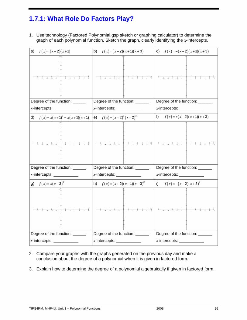
1.7.1: What Role Do Factors Play? 1. Use technology (Factored Polynomial.gsp sketch or graphing calculator) to determine the

graph of each polynomial function. Sketch the graph, clearly identifying the x-intercepts. a) ( ) ( )( )2 1f x x x= − + b) ( ) ( )( )( )2 1 3f x x x x= − + + c) ( ) ( )( )( )2 1 3f x x x x= − − + +

−5 −4 −3 −2 −1 1 2 3 4 5 6

x

y

−5 −4 −3 −2 −1 1 2 3 4 5 6

x

y

−5 −4 −3 −2 −1 1 2 3 4 5 6

x

y

Degree of the function: ______

x-intercepts: ___________





d) ( ) ( ) ( )( )21 1 1f x x x x x x= + = + + e) ( ) ( ) ( )2 22 2f x x x= − + f) ( ) ( )( )( )2 1 3f x x x x x= − + +

−5 −4 −3 −2 −1 1 2 3 4 5 6

x

y

−5 −4 −3 −2 −1 1 2 3 4 5 6

x

y

−5 −4 −3 −2 −1 1 2 3 4 5 6

x

y







g) ( ) ( )33f x x x= − h) ( ) ( )( )( )22 1 3f x x x x= + − − i) ( ) ( )( )32 3f x x x= − − +

−5 −4 −3 −2 −1 1 2 3 4 5 6

x

y

−5 −4 −3 −2 −1 1 2 3 4 5 6

x

y

−5 −4 −3 −2 −1 1 2 3 4 5 6

x

y







2. Compare your graphs with the graphs generated on the previous day and make a

conclusion about the degree of a polynomial when it is given in factored form. 3. Explain how to determine the degree of a polynomial algebraically if given in factored form.


1.7.1: What Role Do Factors Play? 4. What connection do you observe between the factors of the polynomial function and the

x-intercepts? Why does this make sense? (Hint: all co-ordinates on the x-axis have y = 0). 5. Use your conclusions from question 4 to state the x-intercepts of each of the following.

Check by graphing with technology, and correct, if necessary.

( ) ( )( ) 13 52

f x x x x⎛ ⎞= − + −⎜ ⎟⎝ ⎠

( ) ( )( ) ( )3 5 2 1f x x x x= − + − ( ) ( )( )( )( )2 3 2 5 1 3 2f x x x x x= − + − −


Does this check? _______


Does this check? _______


Does this check? _______ 6. What do you notice about the graph when the polynomial function has a factor that occurs

twice? Three times?


1.7.2: Factoring in our Graphs Draw a sketch of each graph using the properties of polynomial functions. After you complete each sketch, check with your partner, discuss your strategies, and make any corrections needed. a) ( ) ( )( )f x x x= − +4 3 b) ( ) ( )( )( )f x x x x= − − + − 1

21 4 c) ( ) ( )( )f x x x= − + 22 1 1

−5 −4 −3 −2 −1 1 2 3 4 5 6

x

y

−5 −4 −3 −2 −1 1 2 3 4 5 6

x

y

−5 −4 −3 −2 −1 1 2 3 4 5 6

x

y

d) ( ) ( )f x x x= − 32 2 e) ( ) ( ) ( )f x x x= − − +2 22 3 2 f) ( ) ( )( )( )f x x x x x= − + +2 1 2 3

−5 −4 −3 −2 −1 1 2 3 4 5 6

x

y

−5 −4 −3 −2 −1 1 2 3 4 5 6

x

y

−5 −4 −3 −2 −1 1 2 3 4 5 6

x

y

g) ( ) ( )f x x x= −3 4 h) ( ) ( ) ( )f x x x= − + −2 33 3 i) ( ) ( )( )( )( )f x x x x x x= + − − +2 1 3 4

−5 −4 −3 −2 −1 1 2 3 4 5 6

x

y

−5 −4 −3 −2 −1 1 2 3 4 5 6

x

y

−5 −4 −3 −2 −1 1 2 3 4 5 6

x

y


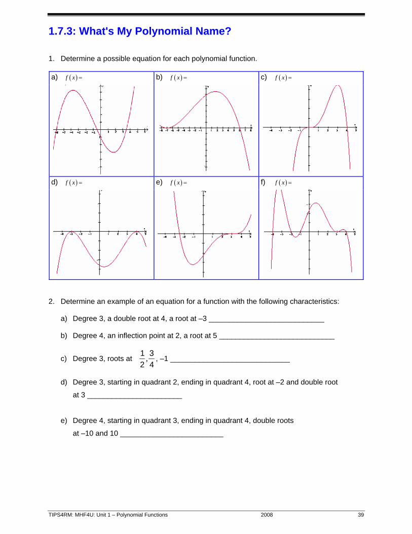
1.7.3: What's My Polynomial Name? 1. Determine a possible equation for each polynomial function. a) ( )f x = b) ( )f x = c) ( )f x =

d) ( )f x = e) ( )f x = f) ( )f x =

2. Determine an example of an equation for a function with the following characteristics:

a) Degree 3, a double root at 4, a root at –3 ____________________________ b) Degree 4, an inflection point at 2, a root at 5 ____________________________

c) Degree 3, roots at ,1 32 4

, –1 _____________________________

d) Degree 3, starting in quadrant 2, ending in quadrant 4, root at –2 and double root

at 3 _______________________

e) Degree 4, starting in quadrant 3, ending in quadrant 4, double roots

at –10 and 10 _________________________


GSP® file Factored Polynomials


Unit 1: Day 8: Transforming Polynomials MHF4U

75 min

Math Learning Goals • Investigate transformations applied to ( ) 3f x x= and ( ) 4.f x x= • Investigate and compare the properties of odd and even functions.


1.8.3, 1.8.4, 1.8.5 • graphing

technology • flash cards,

TI-Navigator, or clickers


Minds On… Individual Anticipation Guide Students review prior knowledge of transformations using BLM 1.8.1.

Curriculum Expectations/Anticipation Guide/Mental Note: Anticipation Guide responses are collected using flash cards, technology or hand signals (a = 1 finger, b = 2 fingers, etc.) once completed. Note which students may need additional support.

Action! Small Groups Exploration Students use their knowledge of transformations to sketch graphs of polynomials and confirm using technology (BLM 1.8.2).

Pairs Investigation Discuss with the class what changes to the function are necessary to create a reflection in the y-axis and a reflection in the x-axis. Students work through BLM 1.8.3 and 1.8.4 with a partner using graphing technology.

Learning Skills/Teamwork/Observation/Checkbric: Observe students’ ability to work collaboratively.

Consolidate Debrief

Whole Class Discussion Lead a class discussion about what observations can be made from BLM 1.8.3 and 1.8.4 to define and draw out key properties of odd and even functions. Pose questions such as: • Which functions look the same after you reflect them over the y-axis? Both

axis? • Which functions have ( ) ( ) ( ) ( )? ?f x f x f x f x− = − = −

What general conclusions can you make about even and odd functions? (Possible Answer: Cubic functions with all odd powers in terms will be odd. Quartic functions with all even powers in terms will be even. A mixture of even and odd powers in a function will be neither even nor odd.) This is a good opportunity to also show students how you can test for even and odd numerically. For example if they check ( )2f and ( )2f − and don’t get the same value then the function isn’t even.

This diagnostic data can also be collected using TI-Navigator or clickers, if available. For Kinaesthetic Learners – Tai Chi movements could be used as an alternative warm-up/diagnostic, .i.e., move upper body and arms to the left; raise arms and body up; show a vertical stretch by having both arms move in opposite directions from the middle.


Home Activity or Further Classroom Consolidation Complete worksheet 1.8.5.


1.8.1: What's the Change? If the graph of a function ( )y f x= is provided, choose the most appropriate description of the change indicated.

1. ( )y f x= + 3 2. ( )y f x= 5

a. shift right b. shift up c. slide left d. slide down

a. vertical compression b. horizontal stretch c. horizontal compression d. shift up

3. ( )y f x= − 4. ( )y f x= 2

a. reflection about x-axis b. reflection about y-axis c. shift down d. slide left

a. horizontal compression and shift right b. horizontal compression and shift left c. vertical stretch and shift right d. horizontal stretch and shift left

5. ( )y f x= −3 6. ( )( ).y f x= +0 5 3

a. horizontal stretch and reflection in x-axis b. horizontal stretch and reflection in y-axis c. vertical stretch and reflection in x-axis d. horizontal stretch and reflection in y-axis

a. horizontal compression and shift right b. horizontal compression and shift left c. vertical stretch and shift right d. horizontal stretch and shift left

7. ( )y f x= + 5 8. ( )y f x= − −

a. vertical shift down b. horizontal shift left c. vertical slide up d. horizontal shift right

a. reflection in x-axis and vertical compression

b. reflection in y-axis and horizontal compression

c. reflection in both axes d. vertical and horizontal compression

9. ( )( )y f x= − + 2 10. ( )y f x= − +1 1 42

a. vertical compression and shift left b. reflection in x-axis and shift right c. reflection in y-axis and shift left d. reflection in y-axis and shift left

a. vertical compression, shift right, shift up b. vertical compression, slide left, shift up c. horizontal compression, shift right and

shift down d. vertical stretch, shift right, shift up


1.8.2: Transforming the Polynomials Using your knowledge of transformations and ( )f x x= 3 or ( )f x x= 4 as the base graphs, sketch the graphs of the following polynomial functions and confirm using technology.

( )f x x= 3 ( )f x x= − 3 ( ) ( )f x x= − 3

( ) ( )f x x= + 31 ( )f x x= −32 1 ( ) ( )f x x= − − +31 14 23

( )f x x= 4 ( )f x x= − 4 ( ) ( )f x x= − 4

( ) ( )f x x= − 42 ( )f x x= − +412 3 ( ) ( )( )f x x= +

42 3

Putting it all together: For ( ) ( )( )f x a k x d c= − +

3and ( ) ( )( ) ,f x a k x d c= − +

4describe the effects of changing a, k, d

and c in terms of transformations.


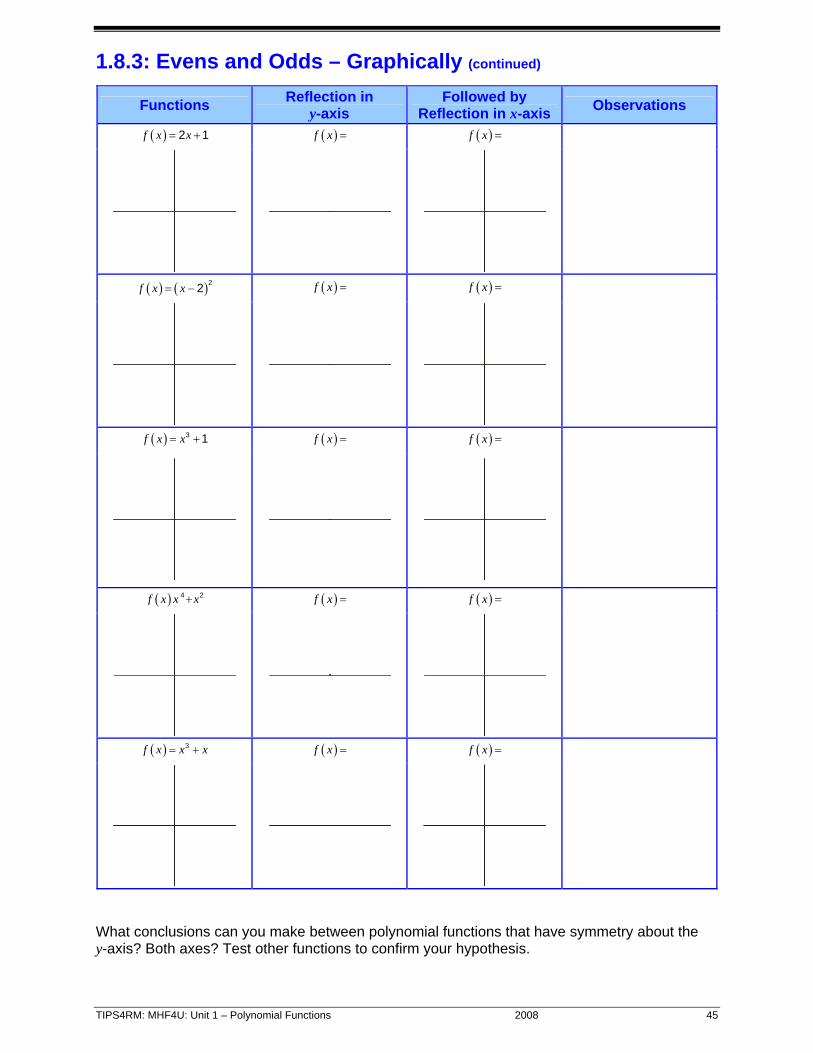
1.8.3: Evens and Odds – Graphically

What transformation reflects a function in the y-axis? _______________________

What transformation reflects a function in the x-axis? _______________________

For each function: • Write the equation that will result in the specified transformation. • Enter the equations into the graphing calculator (to make the individual graphs easier to

view, change the line style on the calculator). • Confirm the equation provides the correct transformation; adjust if needed. • Sketch a graph of the original function and the reflections. • Record any observations you have about the resulting graphs.

Function Reflection in y-axis Followed by reflection in y-axis Observations

( )f x x= ( )f x = ( )f x =

( )f x x= 2 ( )f x x= 2 ( )f x x= − 2

• a reflection in y-axis makes no change in the graph

• a reflection in both axes makes a change in the graph

( )f x x= 3 ( )f x = ( )f x =

( )f x x= 4 ( )f x = ( )f x =


1.8.3: Evens and Odds – Graphically (continued)

Functions Reflection in y-axis

Followed by Reflection in x-axis Observations

( )f x x= +2 1 ( )f x = ( )f x =

( ) ( )f x x= − 22 ( )f x = ( )f x =

( )f x x= +3 1 ( )f x = ( )f x =

( )f x x x+4 2 ( )f x = ( )f x =

( )f x x x= +3 ( )f x = ( )f x =

What conclusions can you make between polynomial functions that have symmetry about the y-axis? Both axes? Test other functions to confirm your hypothesis.


1.8.4: Evens and Odds – Algebraically For each of the functions in the table below find the algebraic expressions for ( )f x− and ( ).f x− Simplify your expressions and record any similarities and differences you see in the algebraic expressions. The second one is done for you as an example.

Function ( )f x− ( )f x− Observations

( )f x x=

( )f x x= 2 2-f(x)= -(x )2= - x

2f(-x)=(-x)2= x

• The expressions for ( )f x− and ( )f x are the

same. • The expressions for

( )f x− and ( )f x are opposites.

( )f x x= 3

( )f x x= 4

( )f x x= +2 1


1.8.4: Evens and Odds – Algebraic (continued)

Function ( )f x− ( )f x− Observations

( ) ( )f x x= − 22

( )f x x= +3 1

( )f x x x= +4 2

( )f x x x= +3

What conclusions can you make between polynomial functions that are the same and different when comparing ( ) ( ),f x f x− and ( )f x− ? Test other functions to confirm your hypothesis.


1.8.5: Evens and Odds – Practice Determine whether each of the functions below is even, odd, or neither. Justify your answers. 1. 2.

3. 4.

5. ( )f x x= +23 4 6. ( )f x x= − +2 5

7. ( )f x x x= +22 3 8. ( )f x x x= − +33

Documents

MHF4U Unit 1 - Ontario€¢ BLM 1.1.1, 1.1.2 Assessment ... the progress of students who had ... TIPS4RM: MHF4U: Unit 1 – Polynomial Functions 2008 8