BROOKINGS | November 2011 1

METROPOLITAN OPPORTUNITY SERIES

The Re-Emergence of Concentrated Poverty: Metropolitan Trends in the 2000sElizabeth Kneebone, Carey Nadeau, and Alan Berube

“ After substantial

progress against

concentrated

poverty during

the booming

economy of the

late 1990s, the

economically

turbulent 2000s

saw much of

those gains

erased.”

FindingsAn analysis of data on neighborhood poverty from the 2005–09 American Community Surveys and Census 2000 reveals that:

■ After declining in the 1990s, the population in extreme-poverty neighborhoods—where at least 40 percent of individuals live below the poverty line—rose by one-third from 2000 to 2005–09. By the end of the period, 10.5 percent of poor people nationwide lived in such neighborhoods, up from 9.1 percent in 2000, but still well below the 14.1 percent rate in 1990.

■ Concentrated poverty nearly doubled in Midwestern metro areas from 2000 to 2005–09, and rose by one-third in Southern metro areas. The Great Lakes metro areas of Toledo, Youngstown, Detroit, and Dayton ranked among those experiencing the largest increases in concentrated poverty rates, while the South was home to metro areas posting both some of the largest increases (El Paso, Baton Rouge, and Jackson) and decreases (McAllen, Virginia Beach, and Charleston). At the same time, concentrated poverty declined in Western metro areas, a trend which may have reversed in the wake of the late 2000s housing crisis.

■ The population in extreme-poverty neighborhoods rose more than twice as fast in sub-urbs as in cities from 2000 to 2005–09. The same is true of poor residents in extreme-pov-erty tracts, who increased by 41 percent in suburbs, compared to 17 percent in cities. However, poor people in cities remain more than four times as likely to live in concentrated poverty as their suburban counterparts.

■ The shift of concentrated poverty to the Midwest and South in the 2000s altered the average demographic profi le of extreme-poverty neighborhoods. Compared to 2000, resi-dents of extreme-poverty neighborhoods in 2005–09 were more likely to be white, native-born, high school or college graduates, homeowners, and not receiving public assistance. However, black residents continued to comprise the largest share of the population in these neighbor-hoods (45 percent), and over two-thirds of residents had a high school diploma or less.

■ The recession-induced rise in poverty in the late 2000s likely further increased the concentration of poor individuals into neighborhoods of extreme poverty. While the con-centrated poverty rate in large metro areas grew by half a percentage point between 2000 and 2005–09, estimates suggest the concentrated poverty rate rose by 3.5 percentage points in 2010 alone, to reach 15.1 percent. Some of the steepest estimated increases compared to 2005–09 occurred in Sun Belt metro areas like Cape Coral, Fresno, Modesto, and Palm Bay, and in Midwestern places like Indianapolis, Grand Rapids, and Akron.

These trends suggest the strong economy of the late 1990s did not permanently resolve the challenge of concentrated poverty. The slower economic growth of the 2000s, followed by the worst downturn in decades, led to increases in neighborhoods of extreme poverty once again throughout the nation, particularly in suburban and small metropolitan communities and in the Midwest. Policies that foster balanced and sustainable economic growth at the regional level, and that forge connections between growing clusters of low-income neighborhoods and regional economic opportunity, will be key to longer-term progress against concentrated disadvantage.

BROOKINGS | November 20112

Introduction

As the fi rst decade of the 2000s drew to a close, the two downturns that bookended the period, combined with slow job growth between, clearly took their toll on the nation’s less fortunate residents. Over a ten-year span, the country saw the poor population grow by 12.3 million, driving the total number of Americans in poverty to a historic high of 46.2

million. By the end of the decade, over 15 percent of the nation’s population lived below the federal poverty line—$22,314 for a family of four in 2010—though these increases did not occur evenly through-out the country.1

The poverty data released each year by the U.S. Census Bureau show us the aggregate level of dis-advantage in America, as well as what parts of the country are more or less affected by poverty. Less

Box 1. Why Does Concentrated Poverty Matter?Being poor in a very poor neighborhood subjects residents to costs and limitations above and beyond the burdens of individual poverty. Summarized in part below, research has shown the wide-ranging social and economic effects that result when the poor are concentrated in economically segregated and disadvantaged neighborhoods.a Concentrated poverty can:

Limit educational opportunity. Children in high-poverty communities tend to go to neighborhood schools where nearly all the students are poor and at greater risk of failure, as measured by standardized tests, dropout rates, and grade retention.b Low performance owes not only to family background, but also to the negative effects high-poverty neighborhoods have on school processes and quality. Teachers in these schools tend to be less experienced, the student body more mobile, and additional sys-tems must often be put in place to deal with the social welfare needs of the student body, creating further demands on limited resources.c

Lead to increased crime rates and poor health outcomes. Crime rates, and particularly violent crime rates, tend to be higher in economically distressed inner-city neighborhoods.d Faced with high crime rates, dilapidated housing stock, and the stress and marginalization of poverty, residents of very poor neighborhoods demonstrate a higher incidence of poor physical and mental health outcomes, like asthma, depression, diabetes, and heart ailments.e

Hinder wealth building. Many residents in extreme-poverty neighborhoods own their home, yet neighborhood conditions in these areas can lead the market to devalue these assets and deny them the ability to accumulate wealth through the apprecia-tions of house prices.f Moreover, the presence of high-poverty neighborhoods can affect residents of the larger metropolitan area generally, depressing values for owner-occupied properties in the region by 13 percent on average.g

Reduce private-sector investment and increase prices for goods and services. High concentrations of low-income and low-skilled households in a neighborhood can make the community less attractive to private investors and employers, which may limit local job opportunities and ultimately create a “spatial mismatch” between low-income residents and employment centers.h In addition, lack of business competition in poor neighborhoods can drive up prices for basic goods and services—like food, car insurance, utilities, and fi nancial services—compared to what families pay in middle-income neighborhoods.i

Raise costs for local government. The concentration of poor individuals and families—which can result in elevated welfare caseloads, high rates of indigent patients at hospitals and clinics, and the need for increased policing—burdens the fi scal capac-ity of local governments and can divert resources from the provision of other public goods. In turn, these dynamics can lead to higher taxes for local businesses and non-poor residents.j

a For a more detailed review of this literature, see “The Enduring Challenge of Concentrated Poverty in America: Case Studies from Communities Across the U.S.” from the Federal Reserve System and the Brookings Institution (Washington: 2008); and Alan Berube and Bruce Katz, “Katrina’s Window: Confronting Concentrated Poverty Across America” (Washington: Brookings Institution, 2005).

b Century Foundation Task Force on the Common School, Divided We Fall: Coming Together Through Public School Choice (New York: Century Foundation Press, 2002); Geoffrey T. Wodtke, David J. Harding, and Felix Elwert, “Neighborhood Effects in Temporal Perspective: The Impact of Long-Term Exposure to Concentrated Disadvantage on High School Graduation.” American Sociological Review 76 (5) (2011): 713–36.

c Ruth Lupton, “Schools in Disadvantaged Areas: Recognising Context and Raising Quality” (London: Centre for the Analysis of Social Exclusion, 2004).d Ingrid Gould Ellen and Margery Austin Turner, “Does Neighborhood Matter? Assessing Recent Evidence,” Housing Policy Debate 8 (4) (1997): 833–66.e See, e.g., Deborah Cohen and others, “Neighborhood Physical Conditions and Health,” Journal of American Public Health 93 (3) (2003): 467–71.f David Rusk, “The Segregation Tax: The Cost of Racial Segregation to Black Homeowners” (Washington: Brookings Institution, 2001).g George Galster, Jackie Cutsinger, and Ron Malega, “The Costs of Concentrated Poverty: Neighborhood Property Markets and the Dynamics of Decline,” in N.

Retsinas and E. Belsky, eds., Revisiting Rental Housing: Policies, Programs, and Priorities (Washington: Brookings Institution, 2008).h Keith Ihlanfeldt and David Sjoquist, “The Spatial Mismatch Hypothesis: A Review of Recent Studies and Their Implications for Welfare Reform.” Housing Policy

Debate 9 (4) (1998): 849–92. i Matthew Fellowes, “From Poverty, Opportunity: Putting the Market to Work for Lower-Income Families” (Washington: Brookings Institution, 2006).j Janet Rothenberg Pack, “Poverty and Urban Public Expenditures,” Urban Studies 35 (11) (1998): 1995–2019.

BROOKINGS | November 2011 3

clear, until now, is how these trends changed the location of poor households within urban, suburban, or rural communities.

Why does the geographic distribution of the poor matter? Rather than spread evenly, the poor tend to cluster and concentrate in certain neighborhoods or groups of neighborhoods within a community. Very poor neighborhoods face a whole host of challenges that come from concentrated disadvan-tage—from higher crime rates and poorer health outcomes to lower-quality educational opportunities and weaker job networks (Box 1).2 A poor person or family in a very poor neighborhood must then deal not only with the challenges of individual poverty, but also with the added burdens that stem from the place in which they live. This “double burden” affects not only the families and individuals bearing it, but also complicates the jobs of policymakers and service providers working to promote connections to opportunity and to alleviate poverty.3

After decades of growth in the number of high-poverty neighborhoods and increasing concentra-tions of the poor in such areas, the booming economy of the 1990s led to a signifi cant de-concentra-tion of American poverty.4 Shortly after the onset of the 2000s, however, that progress seemed to erode as the economy slowed, though until recently researchers have lacked the necessary data to fully assess the changes in the spatial organization of the poor over the last decade.5

After a brief overview of the methods, this paper uses data from the decennial census and American Community Survey to update previous analyses and assess the extent to which concentrations of pov-erty have changed within the United States in the 2000s. We fi rst analyze the trends for the nation as whole, as well as metropolitan and non-metropolitan communities, but focus primarily on changes in concentrated poverty within and across the nation’s 100 largest metropolitan areas, which are home to two-thirds of the nation’s residents and over 60 percent of the country’s poor population.

Methodology

This paper analyzes recent changes in the spatial organization of poverty across the United States. We draw on a well-established body of research to defi ne geographic units of analy-sis, data sources, and key measures of these trends over time.6

GeographiesCensus tracts make up the base units of analysis in this study. The Census Bureau divides the entire United States into tracts, which are meant to delineate relatively homogenous areas that contain roughly 4,000 people on average. They do not always align perfectly with local perceptions of neigh-borhood boundaries, but they provide a reasonable proxy for our purposes. Tract boundaries change over time to refl ect local population dynamics; we use contemporaneous boundaries for each year of data to avoid introducing bias in the neighborhood-level analysis.7

Based on the location of its centriod, each tract is assigned to one of three main geography types using GIS mapping software: large metropolitan areas, small metropolitan areas, and non-metropolitan communities. The U.S. Offi ce of Management and Budget identifi ed 366 metropolitan statistical areas (MSAs) in 2008. Large metropolitan areas include the 100 most populous based on 2008 population estimates, while the remaining 266 regions are designated as small metropolitan areas. Any tract in a county that falls outside of a metropolitan statistical area is considered non-metropolitan.

Within the 100 largest metro areas, we designate primary city and suburban tracts. Primary city tracts include those with a centroid that falls within the fi rst city in the offi cial metropolitan statistical area name, or within any other city in the MSA name with a population over 100,000. In the top 100 metro areas, 137 cities meet the primary city criteria. Suburban tracts make up the remainder of the metropolitan area. We also assign suburban tracts a type based on the urbanization rate of the county (or portion of the county) in which it is located. High density suburbs are those where more than 95 percent of the population lived in an urbanized area in 2000; mature suburbs had urbanization rates of 75 to 95 percent; in emerging suburbs between 25 and 75 percent of the population lived in an urbanized area; and exurbs had urbanization rates below 25 percent in 2000.8

BROOKINGS | November 20114

Key measuresThroughout this study, we use the federal poverty thresholds to measure poverty. The shortcomings of the offi cial poverty measure have been well documented.9 However, the measure provides a stable benchmark—and is reported at a level of detail—that allows for tracking changes in the spatial organi-zation of the poor over time.

To do so, we fi rst measure the incidence of tracts with poverty rates of 40 percent or more in each year, referred to here as extreme-poverty neighborhoods.10 Though any absolute threshold will have its shortcomings (neighborhoods with poverty rates of 39 percent may not differ signifi cantly from those with poverty rates of 41 percent), previous research and policy practice has established the 40 percent parameter as a standard measure by which to designate areas of very high poverty.11

In addition to measuring the total number of residents in extreme-poverty neighborhoods, and the extent to which their characteristics change over time, we also calculate the rate of concentrated poverty, or the share of the poor population located in extreme-poverty tracts. Together these metrics describe not only the prevalence and location of very poor areas within a community, but also the extent to which poor residents in the community are subjected to the “double burden” of being poor in a highly disadvantaged neighborhood.

In addition, we examine trends and characteristics in high-poverty neighborhoods, or those with 20 to 40 percent poverty rates. These tracts do not register in the concentrated poverty rate, but may also experience heightened levels of place-based disadvantage and signal increased clustering of low-income residents in lower-opportunity neighborhoods.

Data sourcesCensus tract data for this analysis come from the decennial censuses in 1990 and 2000, and the American Community Survey (ACS) fi ve-year estimates for 2005–2009.

Key differences exist between the decennial census and the ACS that could affect comparisons. First, the decennial census is a point-in-time survey that asks recipients to report their income for the last year. For example, Census 2000 was administered in April of that year, and its long form asked respondents to report on income in 1999. In contrast, the American Community Survey is a rolling survey that is sent out every month and asks participants to report on their income “in the last 12 months”. The 12 months of data are then combined and adjusted for infl ation to create a single-year estimate. The 2008 ACS estimates, for example, represent a time period that spans from January of 2007 to December of 2008.

Second, the ACS surveys a signifi cantly smaller population (3 million households per year) than the decennial census long form (roughly 16 million households in 2000). To produce statistically reliable estimates for small geographies—like census tracts—multiple years of data must be pooled. The only ACS data set that contains suffi cient sample size to report on census tracts is the fi ve-year estimates. These estimates are based on 60 months’ worth of surveys that ask about income in the past 12 months, meaning they span from January of 2004 through December of 2009. They do not represent any given year, but provide an adjusted estimate for the entire fi ve-year period. This period bridges vastly different points in the economic cycle, starting with a period of recovery and modest growth and ending two years after the onset of the worst downturn since the Great Depression. The combi-nation of such different periods likely mutes the trends studied here. For example, according to ACS single-year estimates, in 2005 the nation’s poverty rate was 13.3 percent. In 2009 it was 14.3 percent. The fi ve-year estimates place the nation’s 2005–09 poverty rate at 13.5 percent, much closer to the 2005 estimate.12

To address the margins of error that accompany the 2005–09 data, we test for statistically signifi -cant differences and present the results throughout the study. To address the potential muting effect of the pooled estimates, we estimate a regression, described in more detail below.

ProjectionsIn light of the much higher poverty rates observed in the 2010 ACS than in the 2005–09 fi ve-year estimates, it is likely that concentrated poverty was also higher that year than across the previous fi ve years. To understand how more recent increases in poverty may have affected concentrated poverty in metro areas, we estimate the relationship between the change in the metropolitan poverty rate and

BROOKINGS | November 2011 5

the change in concentrated poverty rate based on data from 2000 and 2005–09 using the following regression:

CPit – CP

it-1= �

1(P

it – P

it-1) + �

2(SP

it – SP

it-1) + �

where CP is the share of poor residents in extreme-poverty neighborhoods, and “t” and “i” index the year and metro area, respectively; P is the metropolitan poverty rate; SP is the share of the metropoli-tan poor population in suburbs; and � is an error term.

To estimate the likely change in metropolitan concentrated poverty rates between 2005–09 and 2010, we take the coeffi cients derived from this regression and apply them to metropolitan poverty rates and share of the poor in suburbs reported in the ACS estimates for each year.13

While caution must be used with any projection method, we fi nd this model provides a reasonable estimate of the direction in which concentrated poverty likely moved based on changes in metropoli-tan poverty levels.

Findings

A. After declining in the 1990s, the population in extreme-poverty neighborhoods—where at least 40 percent of individuals live below the poverty line—rose by one-third from 2000 to 2005–09. The 1970s and 1980s saw high-poverty neighborhoods proliferate—the number and population in such areas roughly doubled—due to a combination of economic forces and policy decisions.14 In contrast, Census 2000 recorded a signifi cant reversal in the spatial location of the poor population.15 Between 1990 and 2000, the number of extreme-poverty tracts declined by 29 percent, from 2,921 to 2,075 (Table 1). As pockets of poverty diminished, the number of Americans living in these neighborhoods also fell, and the poor population in extreme-poverty tracts fell faster still.

These changes did not simply result from a decline in poverty.16 Over the same time period, the nation’s poverty rate dropped from 13.1 to 12.4 percent—a smaller decline than the decrease in pockets of extreme poverty—but the actual number of poor individuals increased from 31.7 to 33.9 million. Thus the changes signaled a real shift in the types of neighborhoods occupied by poor individuals over that decade.

Very different poverty dynamics marked the 2000s, however. The poor population climbed to 39.5 million in 2005–09, pushing the nation’s poverty rate up to 13.5 percent, and the number of neighbor-hoods with at least 40 percent of residents in poverty climbed by 747. By 2005–09, these neighbor-hoods housed 8.7 million Americans—2.2 million more than at the start of the decade, a one-third increase. Almost half of those residents—4.1 million—were poor. In 2005–09, 10.5 percent of the poor

Table 1. Total Population and Poor Population in Extreme-Poverty Tracts, 1990 to 2005-09

Percent Change**

1990 to 2000 to 1990 to

Extreme-Poverty Tracts* 1990 2000 2005-09 2000 2005-09 2005-09

Total Population 9,101,622 6,574,815 8,735,395 -27.8% 32.9% -4.0%

Poor Population 4,392,749 3,011,893 4,050,538 -31.4% 34.5% -7.8%

Number of Tracts 2,921 2,075 2,822 -29.0% 36.0% -3.4%

*Extreme-poverty tracts have poverty rates of 40 percent or higher.

**All changes signifi cant at the 90 percent confi dence level.

Source: Brookings analysis of decennial census and ACS data

BROOKINGS | November 20116

population lived in extreme-poverty tracts (Figure 1). While the 2005–09 concentrated poverty rate did not reach its 1990 level (14.1 percent), it represents a signifi cant increase over 2000 (9.1 percent) and signals an emerging re-concentration of the poor.

Moreover, increasing concentrations of poverty over the decade were not confi ned to urban areas (Table 2). Over 60 percent of nation’s poor lived in the 100 most populous metropolitan areas in 2005–09, with the remaining 40 percent roughly split between smaller metropolitan areas and non-metro communities. While large metro areas experienced the largest absolute increases in extreme-poverty neighborhoods and concentrated poverty, small metropolitan areas were home to the fastest growth in extreme-poverty tracts and the number of residents living in them, followed by non-metropolitan communities. However, the nation’s most populous metro areas continued to house a disproportionate

Table 2. Total Population and Poor Population in Extreme-Poverty Tracts, by Community Type, 2000 to 2005-09

Number of Extreme- Total Population in Extreme- Poor Population in Extreme-

Poverty Tracts Poverty Tracts Poverty Tracts

Type of Geography 2000 2005-09 % Change 2000 2005-09 % Change 2000 2005-09 % Change

100 Metro Areas 1,536 1,898 23.6 4,935,506 5,903,264 19.6 2,277,193 2,764,587 21.4

Small-metro 351 616 75.5 969,828 1,746,883 80.1 432,643 802,089 85.4

Non-metro 188 308 63.8 669,481 1,085,248 62.1 302,057 483,862 60.2

Distribution Across

Geography Types 2000 2005-09 Change 2000 2005-09 Change 2000 2005-09 Change

100 Metro Areas 74.0% 67.3% -6.8% 75.1% 67.6% -7.5% 75.6% 68.3% -7.4%

Small-metro 16.9% 21.8% 4.9% 14.8% 20.0% 5.2% 14.4% 19.8% 5.4%

Non-metro 9.1% 10.9% 1.9% 10.2% 12.4% 2.2% 10.0% 11.9% 1.9%

*All changes signifi cant at the 90 percent confi dence level.

Source: Brookings analysis of decennial census and ACS data

Figure 1. Share of Total Population and Poor Population in Extreme-Poverty Tracts, 1990 to 2005-09

*All differences signifi cant at the 90 percent confi dence level.

Source: Brookings analysis of decennial census and ACS data

14%

12%

10%

8%

6%

4%

2%

0%1990 2000 2000–05

Total Population Poor Population

3.7%

14.1%

2.4%

9.1%

2.9%

10.5%

BROOKINGS | November 2011 7

share of the nation’s extreme-poverty neighborhoods in 2005–09, and retained the highest concen-trated poverty rate (11.7 percent, compared to 10.9 percent in small metro areas and 6.3 percent in non-metropolitan communities). The remainder of the analysis focuses on changes in the spatial loca-tion of poverty within and across these large regions.

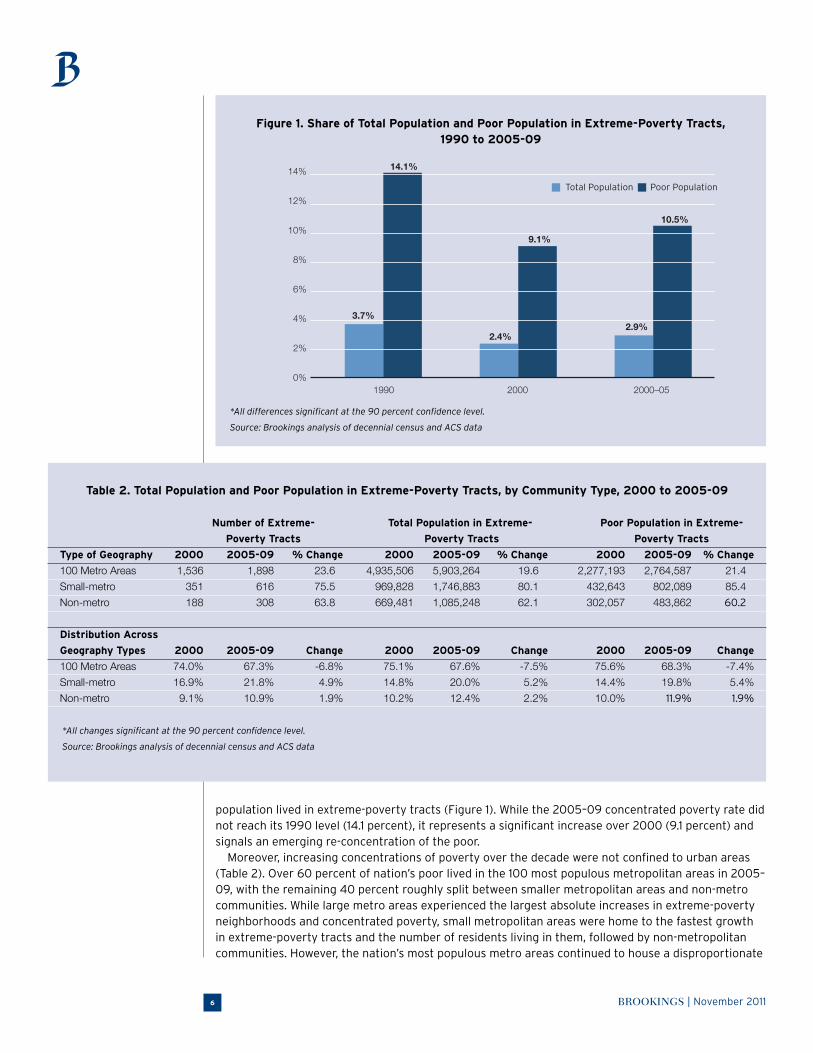
B. Concentrated poverty nearly doubled in Midwestern metro areas from 2000 to 2005–09, and rose by one-third in Southern metro areas. During the 2000s, roughly three-quarters of the nation’s largest metro areas saw their number of extreme-poverty neighborhoods grow, along with the number of poor living in them, compared to just 16 that experienced decreases. The largest increases and decreases tended to cluster in different parts of the country, illuminating larger regional patterns in these trends and tracking with broader changes in poverty across different regions.

The Midwest experienced the most rapid decline in the incidence of extreme-poverty neighborhoods in the 1990s.17 Much of that progress was erased in the 2000s as the Midwest led other regions for growth in pockets of extreme poverty (Table 3). Taken together, Midwestern metro areas registered a 79 percent increase in extreme-poverty neighborhoods in the 2000s. The number of poor living in these tracts almost doubled over the decade, pushing the concentrated poverty rate in the region’s metro areas up by a staggering 5 percentage points, to a level that surpassed that in Northeastern metro areas. While large metro areas like Detroit (30 percent) and Chicago (13 percent) drove some of the growth in the number of poor in extreme-poverty tracts, other major metro areas in the Midwest accounted for the majority of the trend.

Southern metro areas recorded a substantial 33 percent growth in the number of poor individuals in extreme-poverty neighborhoods, though this fi gure masks the steep declines in places like New Orleans and Baltimore that somewhat offset large gains in places like the Texas metro areas of El Paso, Dallas, and Houston. Given the region’s fast growth in overall population and poor residents in the 2000s, and the mixed trajectories of metro areas in different parts of the South, the region’s con-centrated poverty rate rose by a modest 0.8 percentage points.

Northeastern metro areas held steady on these indicators over the decade, while the West actually experienced a drop in concentrated poverty. The Northeast’s trend resulted almost entirely from New York’s signifi cant decrease in the number of poor in extreme-poverty tracts. From 2000 to 2005–09, the number of extreme-poverty tracts in the New York City metropolitan area alone dropped by 64, and poor residents of its extreme-poverty neighborhoods declined by 108,000 poor, effectively can-celling out increases in almost every other Northeastern metro area. Similarly, steep declines in the number of poor in extreme-poverty tracts in Los Angeles, and to some extent, places like San Diego and Riverside, outweighed increases in metro areas like Phoenix, Tucson, Las Vegas, and Denver.

Over the course of the decade, 67 metro areas experienced statistically signifi cant increases in their concentrated poverty rate, compared to decreases in 21 others. Among individual metro areas, the largest increases in the rate of concentrated poverty occurred in the Great Lakes metro areas

Table 3. Total Population and Poor Population in Extreme-Poverty Tracts by Census Region, 100 Metro Areas, 2000 to 2005-09

Number of Extreme-Poverty Tracts Poor Population in Extreme-Poverty Tracts Concentrated Poverty Rate

Region 2000 2005-09 % Change 2000 2005-09 % Change 2000 2005-09 Change

Top 100 Metro Areas 1,536 1,898 23.6% * 2,277,193 2,764,587 21.4% * 11.2% 11.7% 0.5% *

Midwest 344 617 79.4% * 344,958 672,262 94.9% * 10.3% 15.5% 5.2% *

Northeast 452 475 5.1% * 738,579 752,393 1.9% 15.4% 15.2% -0.2%

South 465 576 23.9% * 697,649 930,420 33.4% * 10.6% 11.4% 0.8% *

West 275 230 -16.4% * 496,007 409,512 -17.4% * 8.8% 6.6% -2.2% *

*Change is signifi cant at the 90 percent confi dence level.

Source: Brookings analysis of decennial census and ACS data

BROOKINGS | November 20118

of Toledo, Youngstown, Detroit, and Dayton, and the Northeastern metro areas of New Haven and Hartford (Table 4). Many of these areas saw poverty rise throughout the decade amid the continuing loss of manufacturing jobs.

On the other end of the spectrum, some metro areas in the West and South, like Virginia Beach, Bakersfi eld, Baltimore, and Stockton, exhibited among the largest declines in concentrated poverty rates over the decade.18 However, many of these regions were on the front lines of the housing market collapse and downturn that followed, and recent poverty trends suggest these gains may have been short lived.19 McAllen and Fresno also led for decreases in their concentrated poverty rate in the 2000s, but even with that progress, they rank fi rst and fi fth, respectively, for metropolitan concen-trated poverty rates in 2005–09 (Map 1). They are joined in this regard by other Southern metro areas like El Paso, Memphis, and Jackson, as well as Midwestern metro areas like Detroit, Cleveland, Toledo, and Milwaukee.

C. The population in extreme-poverty neighborhoods rose more than twice as fast in suburbs as in cities from 2000 to 2005–09. Historically, pockets of extreme poverty have been a largely urban phenomenon, though the geog-raphy may be slowly changing for large metro areas. Cities reaped the benefi ts of de-concentrating poverty in the 1990s to a much greater extent than their surrounding suburbs (Table 5).

Extreme-poverty neighborhoods grew in cities and suburbs alike during the 2000s, though the phe-nomenon remained a majority-urban one. In 2005–09, cities contained over 80 percent of extreme-poverty tracts within the nation’s 100 largest metro areas, and had a concentrated poverty rate more

Table 4. Top and Bottom Metro Areas for Change in Concentrated Poverty Rate, 2000 to 2005-09

Metro Areas 2000 to 2005-09

With Greatest Increases in Concentrated Poverty Change in Poor Population in Change in Number of

Concentrated Poverty Rate Change Extreme-Poverty Tracts Extreme-Poverty Tracts

Toledo, OH 15.3% 16,918 15

El Paso, TX 14.5% 33,953 16

Youngstown-Warren-Boardman, OH-PA 14.3% 12,390 11

Baton Rouge, LA 13.5% 16,150 7

Detroit-Warren-Livonia, MI 13.2% 98,940 73

Jackson, MS 12.2% 12,383 11

New Haven-Milford, CT 11.3% 10,834 9

Poughkeepsie-Newburgh-Middletown, NY 10.5% 8,334 0

Dayton, OH 9.9% 11,959 8

Hartford-West Hartford-East Hartford, CT 9.5% 11,023 11

With Greatest Decreases in Concentrated Poverty

New Orleans-Metairie-Kenner, LA -9.3% -29,524 -14

McAllen-Edinburg-Mission, TX -7.3% 11,229 -3

Virginia Beach-Norfolk-Newport News, VA-NC -6.7% -10,234 -7

Fresno, CA -6.6% -11,064 -5

Provo-Orem, UT -6.0% -1,725 1

Bakersfi eld, CA -5.8% -4,291 -3

Baltimore-Towson, MD -5.5% -13,051 -14

Charleston-North Charleston-Summerville, SC -4.9% -2,552 -1

Stockton, CA -4.8% -4,373 0

San Diego-Carlsbad-San Marcos, CA -4.6% -15,641 -8

*All changes signifi cant at the 90 percent confi dence level.

Source: Brookings analysis of decennial census and ACS data

BROOKINGS | November 2011 9

Map 1. Concentrated Poverty Rate, 100 Metro Areas, 2005-09

Concentrated Poverty Rate

<5%5-1

0%

10-15

%15

%<

Table 5. Change in Extreme-Poverty Neighborhoods in Cities and Suburbs, 100 Metro Areas, 1990 to 2005-09

City Suburb

Change Change

Extreme- 2005- 1990 2000 2005- 1990 2000

Poverty Tracts 1990 2000 2009 to 05-09 to 05-09 1990 2000 2009 to 05-09 to 05-09

Total Population 5,174,783 4,027,578 4,662,473 -9.9% 15.8% 900,842 907,928 1,240,791 37.7% 36.7%

Poor Population 2,529,484 1,871,337 2,193,858 -13.3% 17.2% 429,081 405,856 570,729 33.0% 40.6%

Tracts 1,701.00 1,313.00 1,554.00 -8.6% 18.4% 262 223 344 31.3% 54.3%

Share of Total Population 9.5% 6.9% 7.7% -1.8% 0.8% 0.9% 0.8% 0.9% 0.0% 0.2%

Share of Poor Population 26.6% 18.3% 20.0% -6.6% 1.7% 5.1% 4.0% 4.5% -0.6% 0.5%

*All changes signifi cant at the 90 percent confi dence level.

Source: Brookings analysis of decennial census and ACS data

Source: Brookings analysis of decennial census and ACS data

BROOKINGS | November 201110

than four times higher (20 percent) than suburbs (4.5 percent). However, just as suburbs outpaced cities for growth in the poor population as a whole over the

decade, they also saw the number of poor living in extreme-poverty neighborhoods grow faster than in cities.20 The number of extreme-poverty neighborhoods in suburban communities grew by 54 percent, compared to 18 percent in cities, and the poor population living in these suburban neighborhoods rose by 41 percent—more than twice as fast as the 17 percent growth in cities. As a result, though cities still remained better off on these measures in 2005–09 than in 1990, suburbs had surpassed 1990 levels on almost every count.

Growth rates differed across suburbs as well. Higher-density, older suburbs were home to a larger number of extreme-poverty neighborhoods and poor residents living in concentrated poverty than newer, lower-density communities (Table 6). Interestingly, mature suburbs—those that largely devel-oped in the middle decades of the 20th century, in contrast to older “streetcar suburbs” bordering central cities—are home to more extreme-poverty tracts and poor population in those tracts than their more urbanized neighbors. But newer emerging and exurban suburbs experienced the fastest pace of growth among suburbs in concentrated poverty over the decade, albeit from a low base. The trends underscore that just as no category of suburb was immune to broader growth in poverty over the decade, the challenges of concentrated poverty became more regional in scope as well.21

Increases in concentrated poverty were widespread among both cities and suburbs in the 100 larg-est metro areas during the 2000s. Altogether, 61 experienced signifi cant increases in city concentrated poverty rates, compared to 20 with signifi cant decreases. Suburban concentrated poverty rates rose in 54 metro areas and declined in 16 (Table 7). By and large, city and suburban rates moved together over time, but Poughkeepsie and Fresno experienced among the steepest drops in cities concentrated poverty rates even as they topped the list for increases in suburban concentrated poverty rates.

Different factors can cause concentrated poverty to rise or fall in a region: a change in the number of extreme-poverty neighborhoods, growth or decline in the poor population living in these neighbor-hoods, or a combination of the two. Fifty-eight (58) percent of extreme-poverty tracts in cities in 2000 remained extreme-poverty tracts in 2005–09. However, these tracts shed total population and poor residents over the 2000s. The increase in concentrated poverty in cities was thus driven by growth of new pockets of poverty in these urban centers. Just as in cities, 58 percent of suburban extreme-poverty tracts in 2000 remained above the 40 percent threshold in 2005–09. Unlike in cities, those neighborhoods added total residents and poor population over the decade. The rise in suburban concentrated poverty thus refl ected growth in both existing pockets of poverty and the development of new extreme-poverty neighborhoods.

New pockets of poverty that developed in these communities may have been tracts hovering just below the 40 percent threshold in 2000, or others that experienced more signifi cant increases in their poverty rates over the course of the decade. Not refl ected in these numbers are the neighborhoods that saw signifi cant increases in poverty, but did not top the 40 percent threshold in 2005–09. Overall,

Table 6. Change in Extreme Poverty Neighborhoods by Suburban Type, 2000 to 2005-09

Number of Extreme- Total Population Poor Population

Poverty Tracts in Extreme-Poverty Tracts in Extreme-Poverty Tracts

Type of Suburb 2000 2005-09 % Change 2000 2005-09 % Change 2000 2005-09 % Change

Suburban Total 223 344 54.3% 907,928 1,240,791 36.7% 405,856 570,729 40.6%

High Density 79 114 44.3% 304,745 342,375 12.3% 132,628 158,883 19.8%

Mature 100 156 56.0% 450,095 629,557 39.9% 204,842 288,460 40.8%

Emerging 36 58 61.1% 121,603 193,436 59.1% 56,089 93,353 66.4%

Exurb 8 16 100.0% 31,485 75,423 139.6% 12,297 30,033 144.2%

*All changes signifi cant at the 90 percent confi dence level.

Source: Brookings analysis of decennial census and ACS data

BROOKINGS | November 2011 11

cities saw the ranks of the poor in neighborhoods with 20 to 40 percent poverty rates grow by 8 per-cent over the decade, while suburban poor populations in neighborhoods at those poverty levels grew by 41. Research indicates that residents of these neighborhoods experience disadvantages that, while not of the same severity as those affl icting extreme-poverty neighborhoods, may nonetheless limit opportunities and negatively affect their quality of life.22

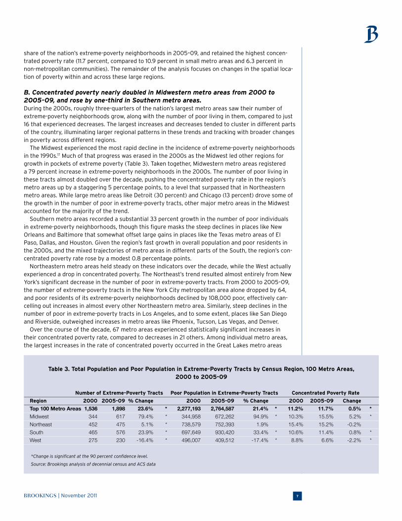
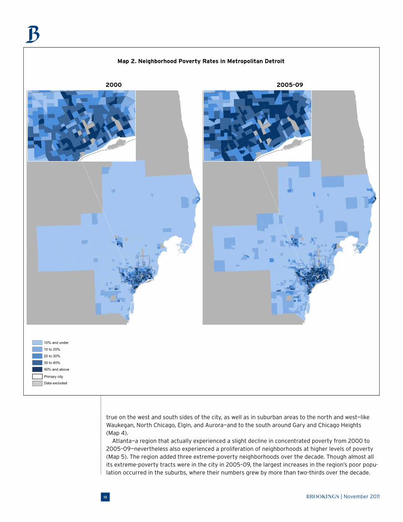
Developing clusters of moderate and higher poverty are evident in places that registered increases in concentrated poverty, like Detroit, Dallas, and Chicago, as well as those that experienced declines. In the Detroit region, as extreme-poverty neighborhoods spread in the cities of Detroit and Warren, and in Oakland County (Pontiac) and St. Clair Counties (Port Huron), scores of other neighborhoods saw poverty rates climb markedly—crossing the 10, 20, and even 30 percent poverty level—in both the inner-ring suburbs and along the metropolitan fringe (Map 2). Jargowsky noted the “bull’s-eye” pattern forming in this region as inner-ring suburbs experienced growing neighborhood poverty even in the strong economy of the 1990s, forecasting the worsening of these patterns in bleaker economic times, along with the potential for these areas to develop similar fi scal and social challenges facing cities with longer histories of concentrated disadvantage.23

Similar patterns played out in the Dallas and Chicago regions. The Dallas region experienced a “fi ll-ing in” in the cities of Dallas and Fort Worth as well as a deepening of suburban pockets of poverty to the northwest around Denton, and northeast along highway 30 (Map 3). At the same time, an increas-ing number of tracts along the metropolitan outskirts crossed the 10 percent threshold. The Chicago region experienced an uptick in extreme-poverty neighborhoods in both the city and suburbs, and saw growing clusters of neighborhoods register moderate to high poverty rates. This was particularly

Table 7. Top and Bottom Metro Areas for Change in Concentrated Poverty Rate, by City and Suburb, 2000 to 2005-09

Change in Concentrated Change in Concentrated

Metro Areas Poverty Rate Metro Areas Poverty Rate

With Greatest Primary City Increases With Greatest Suburban Increases

Bradenton-Sarasota-Venice, FL 36.7% New Haven-Milford, CT 13.8%

Youngstown-Warren-Boardman, OH-PA 36.3% Poughkeepsie-Newburgh-Middletown, NY 13.1%

Portland-South Portland-Biddeford, ME 25.4% Palm Bay-Melbourne-Titusville, FL 10.2%

Dayton, OH 25.2% Cleveland-Elyria-Mentor, OH 8.0%

Detroit-Warren-Livonia, MI 24.3% Baton Rouge, LA 7.0%

Hartford-West Hartford-East Hartford, CT 23.0% Greenville-Mauldin-Easley, SC 6.9%

Jackson, MS 22.4% El Paso, TX 6.7%

Baton Rouge, LA 22.0% Toledo, OH 6.6%

Greenville-Mauldin-Easley, SC 19.6% Fresno, CA 6.5%

Toledo, OH 19.4% Youngstown-Warren-Boardman, OH-PA 6.4%

With Greatest Primary City Decreases With Greatest Suburban Decreases

Provo-Orem, UT -15.4% Tucson, AZ -9.3%

Fresno, CA -13.9% McAllen-Edinburg-Mission, TX -9.0%

Poughkeepsie-Newburgh-Middletown, NY -12.2% Bakersfi eld, CA -6.4%

New Orleans-Metairie-Kenner, LA -11.6% Ogden-Clearfi eld, UT -5.1%

Providence-New Bedford-Fall River, RI-MA -9.6% Virginia Beach-Norfolk-Newport News, VA-NC -4.4%

Scranton--Wilkes-Barre, PA -9.4% Miami-Fort Lauderdale-Pompano Beach, FL -3.8%

San Diego-Carlsbad-San Marcos, CA -9.3% Sacramento--Arden-Arcade--Roseville, CA -3.6%

Charleston-North Charleston-Summerville, SC -8.4% Charleston-North Charleston-Summerville, SC -3.2%

Virginia Beach-Norfolk-Newport News, VA-NC -8.1% Cape Coral-Fort Myers, FL -2.5%

Baltimore-Towson, MD -7.2% Los Angeles-Long Beach-Santa Ana, CA -2.1%

*All changes signifi cant at the 90 percent confi dence level.

Source: Brookings analysis of decennial census and ACS data

BROOKINGS | November 201112

true on the west and south sides of the city, as well as in suburban areas to the north and west—like Waukegan, North Chicago, Elgin, and Aurora—and to the south around Gary and Chicago Heights (Map 4).

Atlanta—a region that actually experienced a slight decline in concentrated poverty from 2000 to 2005–09—nevertheless also experienced a proliferation of neighborhoods at higher levels of poverty (Map 5). The region added three extreme-poverty neighborhoods over the decade. Though almost all its extreme-poverty tracts were in the city in 2005–09, the largest increases in the region’s poor popu-lation occurred in the suburbs, where their numbers grew by more than two-thirds over the decade.

2000 2005-09

Map 2. Neighborhood Poverty Rates in Metropolitan Detroit

10% and under

10 to 20%

20 to 30%

30 to 40%

40% and above

Primary city

Data excluded

BROOKINGS | November 2011 13

As this growth took place, an increasing number of neighborhoods crossed not just the 10 percent poverty mark, but many reached poverty rates of more than 20 or 30 percent by 2005–09 in places to south like Macon, to the northwest towards Marietta, and to the east in areas like Lawrenceville and Gainesville.

In short, concentrated poverty trends in the 2000s appear to have erased some of the progress made in central cities during the 1990s, while accelerating and spreading the growth of higher-poverty suburban communities witnessed that decade.

2000 2005-09

Map 3. Neighborhood Poverty Rates in Metropolitan Dallas

10% and under

10 to 20%

20 to 30%

30 to 40%

40% and above

Primary city

Data excluded

BROOKINGS | November 201114

10% and under

10 to 20%

20 to 30%

30 to 40%

40% and above

Primary city

Data excluded

2000 2005-09

Map 4. Neighborhood Poverty Rates in Metropolitan Chicago

BROOKINGS | November 2011 15

2000 2005-09

Map 5. Neighborhood Poverty Rates in Metropolitan Atlanta

10% and under

10 to 20%

20 to 30%

30 to 40%

40% and above

Primary city

Data excluded

BROOKINGS | November 201116

D. The shift of concentrated poverty to the Midwest and South in the 2000s coincided with changes in the demographic profi le of extreme-poverty neighborhoods. As concentrations of poverty increased and spread in the 2000s, the makeup of extreme-poverty neighborhoods shifted across a number of characteristics (Table 8). In particular, the traditional picture of extreme-poverty neighborhoods has been colored by research and public discussion of the urban “underclass”, a term which has fallen out of favor in recent years but, according to Ricketts and Sawhill, is meant to describe a subset of the population that “suffers from multiple social ills that are concentrated in depressed inner-city areas.”24

Past research has identifi ed four factors to proxy “underclass” characteristics at the neighborhood level: the share of teenagers dropping out of high school, the proportion of households headed by single-mothers, the share of able-bodied men not in the labor force, and the proportion of house-holds on public assistance. During the 2000s, the share of working-age men not in the labor force in extreme-poverty neighborhoods fell by 7 percentage points, as did the share of teenagers in these neighborhoods not in school and without a diploma. The share of households receiving public assis-tance dropped by more than 8 percentage points, and a smaller share were headed by single mothers than at the start of the decade. These shifts underscore an observation made by Ricketts and Sawhill that, while “extreme poverty areas can reasonably be used as a proxy for concentrations of social problems…they are not the same thing.”25

In addition, by 2005–09, residents of extreme-poverty neighborhoods were more likely to be white and less likely to be Latino than in 2000, though African Americans remained the single largest group in these areas (44.6 percent).26 The population in extreme-poverty tracts was also less likely to be foreign born, and residents were more likely to own their homes than at the start of the decade. Compared to 2000, by the last half of the decade residents of these neighborhoods were also better

Table 8. Change in Neighborhood Characteristics in Extreme-Poverty Tracts, 100 Metro Areas, 2000 to 2005-09

Share of individuals: 2000 2005-09

Who are:

White 11.2% 16.5%

Black 45.6% 44.6%

Latino 37.4% 33.9%

Other 5.9% 5.1%

Who are foreign born 20.0% 17.9%

25 and over who have completed:

Less than High School 50.0% 37.9%

High School 25.9% 31.9%

Some College or Associates Degree 17.4% 20.5%

BA or Higher 6.7% 9.7%

Who are 22 to 64 year-old males not in the labor force 39.8% 32.4%

16 to 19 year olds not in school and without a diploma 20.6% 13.6%

Share of households:

That are owner occupied 24.4% 29.3%

That receive public assistance 18.0% 9.6%

Headed by women with children 26.8% 22.5%%

*All changes signifi cant at the 90 percent confi dence level.

Source: Brookings analysis of decennial census and ACS data

BROOKINGS | November 2011 17

educated—more had fi nished high school (31.9 percent) and a higher share held bachelor’s degrees (9.7 percent).

These changes may capture in part the rapid growth of concentrated poverty in the Midwest, which accompanied the economic struggles of regions like Detroit, Toledo, Chicago, and Dayton across the decade. Concentrated poverty in these metro areas spread beyond the urban core to what might previ-ously have been considered working-class areas. Poor local labor market conditions may have pushed up poverty rates across a more demographically and economically diverse set of neighborhoods than traditional “underclass” areas. The same may apply to the South, where the rapid spread of high-poverty neighborhoods to suburban areas amid the housing market downturn further alters long-held notions of concentrated poverty. At the same time, “underclass” characteristics may themselves have become less concentrated as broader swaths of metropolitan areas diversifi ed economically and demographically.

Within major metro areas, extreme-poverty neighborhoods in cities and suburbs share a similar overall demographic and economic profi le. An exception is their racial and ethnic makeup—refl ecting larger differences in the racial and ethnic profi le of cities and suburbs, in that suburban residents of extreme-poverty neighborhoods are more likely to be white and Latino than their counterparts in cit-ies—and a higher homeownership rate in the suburbs.

Greater demographic and economic differences emerge between neighborhoods with poverty rates of at least 40 percent on the one hand, and those with poverty rates between 20 to 40 percent on the other. The latter group housed more than one-third of the metropolitan poor population in 2005–09, compared to about one-tenth of metropolitan poor in the former group.

Residents of high-poverty neighborhoods in 2005–09 were more likely to be white and Latino, and less likely to be African American than the population in extreme-poverty tracts (Table 9). They were

Table 9. Neighborhood Characteristics by Poverty Rate Category, 100 Metro Areas, 2005-09

Share of individuals: In Extreme-Poverty Tracts In High-Poverty Tracts Total Population

Who are:

White 16.5% 29.9% 59.7%

Black 44.6% 27.5% 13.7%

Latino 33.9% 35.6% 18.4%

Other 5.1% 6.9% 8.2%

Who are foreign born 17.9% 23.4% 16.2%

25 and over who have completed:

Less than High School 37.9% 29.2% 14.8%

High School 31.9% 30.8% 26.8%

Some College or Associates Degree 20.5% 23.9% 27.3%

BA or Higher 9.7% 16.1% 31.1%

Who are 22 to 64 year-old males not in the labor force 32.4% 20.1% 14.4%

16 to 19 year olds not in school and without a diploma 13.6% 11.5% 6.5%

Share of households:

That are owner occupied 29.3% 42.8% 65.1%

That receive public assistance 9.6% 5.2% 2.4%

Headed by women with children 22.5% 13.7% 8.1%

*All differences signifi cant at the 90 percent confi dence level.

Source: Brookings analysis of ACS data

BROOKINGS | November 201118

also more likely to be foreign born. Residents of high-poverty neighborhoods exhibited higher levels of education than those in extreme-poverty tracts, with a much higher share of college graduates as well as those who attended some college or hold an associate’s degree. And high-poverty tract residents are much less likely to exhibit the four “underclass” characteristics than their counterparts in extreme-poverty neighborhoods. However, when the benchmark is the metropolitan population as a whole, high-poverty neighborhoods continue to exhibit higher use of public assistance and trail behind the general population on educational attainment, dropout rates, single-mother households, and male attachment to the labor force.

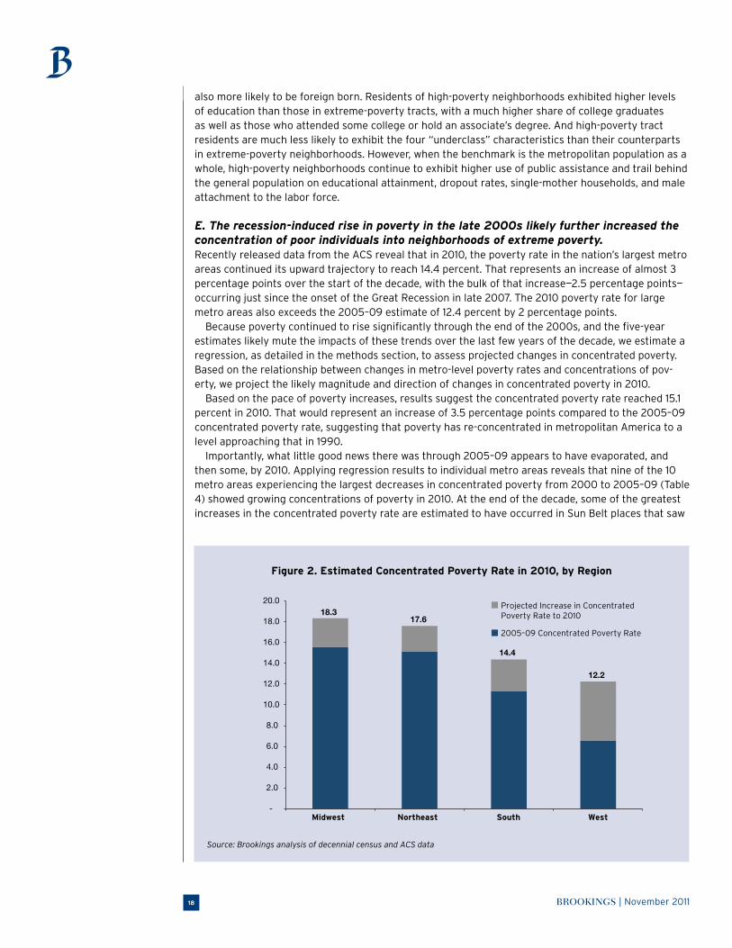
E. The recession-induced rise in poverty in the late 2000s likely further increased the concentration of poor individuals into neighborhoods of extreme poverty. Recently released data from the ACS reveal that in 2010, the poverty rate in the nation’s largest metro areas continued its upward trajectory to reach 14.4 percent. That represents an increase of almost 3 percentage points over the start of the decade, with the bulk of that increase—2.5 percentage points—occurring just since the onset of the Great Recession in late 2007. The 2010 poverty rate for large metro areas also exceeds the 2005–09 estimate of 12.4 percent by 2 percentage points.

Because poverty continued to rise signifi cantly through the end of the 2000s, and the fi ve-year estimates likely mute the impacts of these trends over the last few years of the decade, we estimate a regression, as detailed in the methods section, to assess projected changes in concentrated poverty. Based on the relationship between changes in metro-level poverty rates and concentrations of pov-erty, we project the likely magnitude and direction of changes in concentrated poverty in 2010.

Based on the pace of poverty increases, results suggest the concentrated poverty rate reached 15.1 percent in 2010. That would represent an increase of 3.5 percentage points compared to the 2005–09 concentrated poverty rate, suggesting that poverty has re-concentrated in metropolitan America to a level approaching that in 1990.

Importantly, what little good news there was through 2005–09 appears to have evaporated, and then some, by 2010. Applying regression results to individual metro areas reveals that nine of the 10 metro areas experiencing the largest decreases in concentrated poverty from 2000 to 2005–09 (Table 4) showed growing concentrations of poverty in 2010. At the end of the decade, some of the greatest increases in the concentrated poverty rate are estimated to have occurred in Sun Belt places that saw

Figure 2. Estimated Concentrated Poverty Rate in 2010, by Region

Source: Brookings analysis of decennial census and ACS data

-

2.0

4.0

6.0

8.0

10.0

12.0

14.0

16.0

18.0

20.0

Midwest Northeast South West

Projected Increase in Concentrated Poverty Rate to 2010

2005–09 Concentrated Poverty Rate

18.3 17.6

14.4

12.2

BROOKINGS | November 2011 19

poverty rates climb after the collapse of the housing market and subsequent downturn (Cape Coral, Fresno, Modesto, Palm Bay, Riverside, and Las Vegas), but also in Midwestern metro areas like Grand Rapids, Akron, and Indianapolis.

Taken together, Western metro areas experienced the largest growth in their rate of concen-trated poverty from 2005–09 to 2010, followed by the South (Figure 2). Although Midwestern and Northeastern metro areas saw smaller increases, metro areas in those regions remained home to the highest concentrations of poverty. Ultimately, all but nine metro areas (Baton Rouge, El Paso, Honolulu, Jackson, Kansas City, Knoxville, Madison, McAllen, and San Antonio) are estimated to have experienced an uptick in concentrated poverty in 2010, with 50 metro areas registering increases greater than the average of 3.5 percentage points.

Conclusion

The fi ndings here confi rm what earlier studies this decade suggested: After substantial prog-ress against concentrated poverty during the booming economy of the late 1990s, the eco-nomically turbulent 2000s saw much of those gains erased. Success stories from the 1990s like Chicago and Detroit were on the front lines of re-concentrating poverty in the 2000s,

and they and other areas such as Atlanta and Dallas also saw concentrated poverty spread to new communities. In cities, concentrated poverty had not yet returned to 1990 levels by 2005–09. However, suburbs—home to the steepest increases in the poor population over the decade—cannot say the same.

What is more, the fi ve-year estimates likely downplay the severity of the upturn in these trends because they pool such different time periods together. Estimates of concentrated poverty trends to 2010 indicate that the positive shifts seen in many Sun Belt metro areas through 2005–09 may have evaporated in the wake of the Great Recession and the severe economic dislocation it caused.

There is also evidence that, as poverty has increasingly suburbanized this decade, new clusters of low-income neighborhoods have emerged beyond the urban core in many of the nation’s largest metro areas. The proposition of being poor in a suburb may bring benefi ts to residents if it means they are located in neighborhoods that offer greater access to opportunities—be it better schools, affordable housing, or more jobs—than they would otherwise fi nd in an urban neighborhood. But research has shown that, instead, the suburban poor often end up in lower-income communities with less access to jobs and economic opportunity, compared to higher-income suburbanites.27 Thus, rather than increased opportunities and connections, being poor in poor suburban neighborhoods may mean residents face challenges similar to those that accompany concentrated disadvantage in urban areas, but with the added complication that even fewer resources are likely to exist than one might fi nd in an urban neighborhood with access to a more robust and developed safety net. Yet, as poverty continues to suburbanize and to concentrate, absent policy intervention the suburbs are poised to become home to the next wave of concentrating disadvantage.

Given that a strong economic recovery has failed to materialize, and threats of a double-dip reces-sion loom, it is unlikely the nation has seen the end of poverty’s upward trend. Trends from the past decade strongly indicate that it is diffi cult to make progress against concentrated poverty while poverty itself is on the rise. It is also unlikely that without fundamental changes in how regions plan for things like land use, zoning, housing, and workforce and economic development that the growth of extreme-poverty neighborhoods and concentrated poverty will abate. With cities and suburbs increas-ingly sharing in the challenges of concentrated poverty, regional economic development strategies must do more to encourage balanced growth with opportunities for workers up and down the eco-nomic ladder. Metropolitan leaders must also actively foster economic integration throughout their regions, and forge stronger connections between poor neighborhoods and areas with better education and job opportunities, so that low-income residents are not left out or left behind in the effort to grow the regional economy.

BROOKINGS | November 201120

Appen

dix

A. C

on

cen

trate

d P

over

ty, 10

0 L

arg

est

Met

ropolita

n A

reas,

20

00

to 2

00

5–0

9

2

00

5–0

9

Ch

an

ge

from

20

00

Popu

la-

Ran

k fo

r

Popu

la-

ti

on

in

P

oor

in C

on

cen

- C

on

cen

-

tion

in

Poor

in

Con

cen

-

E

xtr

eme-

Extr

eme-

E

xtr

eme-

tr

ate

d

trate

d

Extr

eme-

E

xtr

eme-

E

xtr

eme-

trate

d

R

an

k fo

r

Tota

l P

oor

Pov

erty

P

over

ty

Pov

erty

Pov

erty

P

over

ty

Pov

erty

P

over

ty

P

over

ty

Pov

erty

C

han

ge

in

M

etro

Are

a

Popu

lati

on

P

opu

lati

on

Tr

act

s Tr

act

s Tr

act

s R

ate

R

ate

Tr

act

s Tr

act

s

Tract

s

Rate

C.P

. R

ate

100

Larg

est

Met

ro A

reas

19

5,85

9,88

1

23,6

64,0

93

1,89

8

5,90

3,26

4

2,76

4,58

7

11.7

%

36

2

967,

758

*

487,

394

* 0.

5% *

Akr

on, O

H

686

,568

8

5,09

0

13

2

3,54

7

11,

466

13

.5%

3

2

9 14

,681

*

7,72

7 *

7.6%

* 17

Alb

any,

NY

8

36,0

01

83,

913

8

2

4,33

4

11,

418

13

.6%

3

1

3 11

,662

*

5,95

3 *

6.1%

* 22

Alb

uque

rque

, NM

8

25,6

80

121

,396

7

2

1,83

2

9,1

14

7.5%

6

6

4 10

,833

*

3,96

6 *

2.3%

* 55

Alle

ntow

n, P

A-N

J 7

99,1

68

70,

597

5

1

4,96

6

6,9

41

9.8%

4

9

1 5,

905

* 2,

782

* 2.

7% *

48

Atla

nta,

GA

5

,213

,776

6

14,1

21

31

8

2,06

4

39,

519

6.

4%

73

3

-2,4

56

-959

-3

.8%

* 76

Aug

usta

-Ric

hmon

d C

ount

y, G

A-S

C

528

,174

8

6,74

0

11

3

6,51

4

16,

025

18

.5%

1

9

3 13

,865

*

5,42

8 *

4.3%

* 32

Aus

tin, T

X 1

,551

,763

1

92,9

24

8

45,

435

2

1,16

6

11.0

%

40

5

23,9

57 *

11

,244

*

3.1%

* 43

Bak

ersfi

eld

, CA

7

80,8

75

151

,223

1

0

53,

254

2

4,51

4

16.2

%

21

-3

-1

1,58

3 *

-4,2

91 *

-5

.8%

* 83

Bal

timor

e, M

D

2,6

48,3

47

241

,499

1

6

39,

691

1

9,51

2

8.1%

6

1

-14

-29,

350

* -1

3,05

1 *

-5.5

% *

82

Bat

on R

ouge

, LA

7

40,1

11

115

,641

1

5

56,

285

2

6,25

4

22.7

%

11

8

33,0

36 *

16

,151

*

13.5

% *

4

Birm

ingh

am, A

L 1

,130

,960

1

47,0

58

11

3

4,41

4

16,

016

10

.9%

4

2

1 89

3

916

0.

1%

Boi

se C

ity, I

D

574

,086

6

6,94

7

2

4,7

31

1,6

87

2.5%

9

2

2 4,

731

* 1,

687

* 2.

5% *

52

Bos

ton-

Cam

brid

ge, M

A-N

H

4,4

19,4

84

390

,554

1

8

51,

816

2

3,80

2

6.1%

7

6

6 24

,773

*

11,5

97 *

2.

6% *

50

Bra

dent

on, F

L 6

80,4

57

71,

456

1

5

,269

1

,952

2.

7%

91

1

5,26

9 *

1,95

2 *

2.7%

* 47

Brid

gepo

rt-S

tam

ford

, CT

883

,254

6

5,43

4

6

12,

312

5

,732

8.

8%

54

3

6,04

4 *

2,85

4 *

3.9%

* 34

Buf

falo

, NY

1

,119

,517

1

48,7

37

19

4

7,44

3

23,

322

15

.7%

2

4

3 -3

,430

*

723

-1

.1%

* 69

Cap

e C

oral

, FL

573

,537

5

9,14

7

1

4,5

79

2,5

72

4.3%

8

2

0 -2

64

-241

-2

.3%

* 73

Cha

rlest

on, S

C

623

,459

8

4,33

4

8

14,

954

6

,934

8.

2%

58

-1

-6

,325

*

-2,5

52 *

-4

.9%

* 81

Cha

rlott

e, N

C-S

C

1,6

29,5

66

189

,714

8

2

0,14

9

10,

309

5.

4%

80

5

13,2

59 *

7,

631

* 3.

2% *

42

Cha

ttan

ooga

, TN

-GA

5

11,9

34

70,

700

9

2

0,48

4

10,

535

14

.9%

2

6

5 9,

051

* 4,

205

* 3.

5% *

39

Chi

cago

-Nap

ervi

lle-J

olie

t, IL

-IN

-WI

9,4

01,7

69

1,1

01,9

42

144

3

41,0

86

158

,746

14

.4%

2

8

39

112,

278

* 41

,544

*

1.7%

* 62

Cin

cinn

ati,

OH

-KY-

IN

2,1

15,0

00

238

,277

3

5

68,

091

3

3,99

6

14.3

%

29

13

21

,078

*

9,57

1 *

0.8%

Cle

vela

nd, O

H

2,0

83,8

12

276

,762

6

6

128

,724

6

4,91

9

23.5

%

7

24

58,2

27 *

30

,376

*

8.0%

* 15

Col

orad

o S

prin

gs, C

O

597

,471

6

0,82

5

2

5,3

37

2,2

04

3.6%

8

6

1 3,

486

* 1,

573

* 2.

1% *

57

Col

umbi

a, S

C

709

,352

8

8,29

3

6

18,

622

5

,985

6.

8%

69

2

7,89

5 *

1,91

4 *

1.3%

* 65

Col

umbu

s, O

H

1,7

28,2

12

212

,111

2

5

57,

225

2

9,00

9

13.7

%

30

17

35

,680

*

19,0

10 *

6.

7% *

20

Dal

las-

Fort

Wor

th-A

rling

ton,

TX

6,1

13,9

88

790

,228

3

9

135

,123

6

4,44

5

8.2%

5

9

16

66,6

36 *

36

,498

*

3.0%

* 44

BROOKINGS | November 2011 21

Day

ton,

OH

8

20,0

54

104

,125

1

4

36,

522

1

6,83

7

16.2

%

22

8

24,6

44 *

11

,959

*

9.9%

* 9

Den

ver-

Aur

ora,

CO

2

,449

,725

2

70,4

99

7

21,

936

1

0,90

6

4.0%

8

4

5 17

,383

*

8,37

4 *

2.5%

* 51

Des

Moi

nes,

IA

543

,541

4

6,73

3

1

3,0

65

1,3

33

2.9%

9

0

1 3,

065

* 1,

333

* 2.

9% *

45

Det

roit-

War

ren,

MI

4,4

46,5

39

624

,278

1

23

303

,931

1

47,4

78

23.6

%

6

73

195,

690

* 98

,940

*

13.2

% *

5

El P

aso,

TX

729

,396

1

90,2

32

32

1

40,7

54

66,

319

34

.9%

2

16

74

,328

*

33,9

53 *

14

.5%

* 2

Fres

no, C

A

888

,955

1

82,1

50

18

1

01,8

27

45,

635

25

.1%

5

-5

-1

8,65

8 *

-11,

064

* -6

.6%

* 85

Gra

nd R

apid

s, M

I 7

73,4

27

98,

401

6

1

6,59

6

7,7

36

7.9%

6

2

3 10

,928

*

5,23

2 *

3.9%

* 36

Gre

ensb

oro-

Hig

h P

oint

, NC

6

86,3

43

105

,164

8

2

6,99

9

12,

726

12

.1%

3

6

7 21

,816

*

10,4

99 *

8.

7% *

11

Gre

envi

lle, S

C

596

,526

8

4,64

2

8

20,

750

9

,088

10

.7%

4

5

6 16

,838

*

7,60

2 *

8.2%

* 13

Har

risbu

rg, P

A

524

,399

4

5,54

3

3

11,

864

5

,576

12

.2%

3

5

1 5,

338

* 2,

679

* 4.

9% *

28

Har

tford

, CT

1,1

68,0

38

103

,104

1

9

46,

557

2

0,55

0

19.9

%

17

11

26

,799

*

11,0

23 *

9.

5% *

10

Hon

olul

u, H

I 8

99,2

31

77,

479

4

8

,118

3

,864

5.

0%

81

0

258

-1

51

0.2%

Hou

ston

, TX

5,5

84,4

54

824

,410

4

7

204

,666

9

0,23

7

10.9

%

41

22

11

7,81

7 *

52,2

29 *

5.

0% *

27

Indi

anap

olis

, IN

1

,688

,592

1

92,2

75

12

3

0,56

2

14,

860

7.

7%

64

9

25,5

65 *

12

,711

*

6.0%

* 23

Jack

son,

MS

5

30,1

04

91,

945

1

8

44,

548

2

0,89

2

22.7

%

10

11

25

,437

*

12,3

83 *

12

.2%

* 6

Jack

sonv

ille, F

L 1

,294

,684

1

47,8

89

11

3

4,92

8

14,

712

9.

9%

47

4

16,4

16 *

6,

843

* 3.

3% *

41

Kan

sas

City

, MO

-KS

2

,009

,042

2

10,3

14

29

5

2,03

0

23,

677

11

.3%

3

8

18

35,4

90 *

16

,758

*

6.8%

* 19

Kno

xville

, TN

6

62,7

01

88,

829

1

0

27,

539

1

3,34

8

15.0

%

25

3

12,9

65 *

6,

453

* 5.

2% *

26

Lake

land

, FL

566

,333

7

9,36

8

4

11,

762

4

,781

6.

0%

77

3

9,12

7 *

3,43

9 *

3.8%

* 37

Las

Vega

s, N

V

1,8

20,4

22

195

,601

8

3

6,09

5

14,

059

7.

2%

67

7

32,5

94 *

12

,639

*

6.2%

* 21

Litt

le R

ock,

AR

6

57,4

46

91,

669

6

1

6,92

9

7,0

74

7.7%

6

5

3 12

,197

*

4,77

0 *

4.5%

* 31

Los

Ang

eles

-Lon

g B

each

-

S

anta

Ana

, CA

1

2,68

2,00

6

1,7

52,7

90

72

2

91,7

75

136

,038

7.

8%

63

-5

4 -2

34,5

99 *

-1

00,4

60 *

-4

.4%

* 78

Loui

sville

/Jef

fers

on C

ount

y, K

Y-IN

1

,233

,293

1

57,9

64

19

5

4,72

1

26,

661

16

.9%

2

0

7 16

,771

*

6,99

8 *

1.0%

Mad

ison

, WI

522

,465

4

5,02

5

McA

llen,

TX

702

,697

2

50,7

66

33

2

81,5

20

133

,471

53

.2%

1

-3

19

,051

*

11,2

29 *

-7

.3%

* 87

Mem

phis

, TN

-MS

-AR

1

,280

,979

2

30,2

74

48

1

33,3

30

63,

818

27

.7%

3

13

55

,004

*

28,0

04 *

8.

2% *

14

Mia

mi-F

ort L

aude

rdal

e-

P

ompa

no B

each

, FL

5,4

78,0

57

751

,149

2

4

96,

341

4

7,43

1

6.3%

7

5

-16

-61,

180

* -2

4,34

4 *

-4.1

% *

77

Milw

auke

e, W

I 1

,527

,440

1

86,0

79

45

9

0,04

4

43,

610

23

.4%

9

8

21,2

77 *

12

,437

*

2.8%

* 46

Min

neap

olis

-St.

Pau

l, M

N-W

I 3

,164

,314

2

66,6

54

19

5

3,09

5

24,

997

9.

4%

52

8

19,9

66 *

12

,248

*

2.7%

* 49

Mod

esto

, CA

5

05,1

65

75,

144

4

1

5,77

5

7,0

83

9.4%

5

1

2 6,

405

* 2,

978

* 3.

6% *

38

Nas

hville

-Dav

idso

n, T

N

1,5

09,3

60

182

,820

1

2

32,

164

1

4,77

9

8.1%

6

0

6 15

,576

*

5,60

8 *

1.1%

* 67

New

Hav

en, C

T 8

36,6

04

87,

063

1

3

40,

231

1

7,21

6

19.8

%

18

9

23,6

94 *

10

,834

*

11.3

% *

7

New

Orle

ans,

LA

1

,140

,551

1

77,1

78

34

4

8,96

0

23,

270

13

.1%

3

3

-14

-57,

943

* -2

9,52

4 *

-9.3

% *

88

BROOKINGS | November 201122

Appen

dix

A. C

on

cen

trate

d P

over

ty, 10

0 L

arg

est

Met

ropolita

n A

reas,

20

00

to 2

00

5–0

9 (

con

tin

ued

)

2

00

5–0

9

Ch

an

ge

from

20

00

Popu

la-

Ran

k fo

r

Popu

la-

ti

on

in

P

oor

in C

on

cen

- C

on

cen

-

tion

in

Poor

in

Con

cen

-

E

xtr

eme-

Extr

eme-

E

xtr

eme-

tr

ate

d

trate

d

Extr

eme-

E

xtr

eme-

E

xtr

eme-

trate

d

R

an

k fo

r

Tota

l P

oor

Pov

erty

P

over

ty

Pov

erty

Pov

erty

P

over

ty

Pov

erty

P

over

ty

P

over

ty

Pov

erty

C

han

ge

in

M

etro

Are

a

Popu

lati

on

P

opu

lati

on

Tr

act

s Tr

act

s Tr

act

s R

ate

R

ate

Tr

act

s Tr

act

s

Tract

s

Rate

C.P

. R

ate

New

Yor

k-N

orth

ern

New

Jer

sey,

N

Y-N

J-PA

1

8,83

0,01

6

2,3

08,9

09

200

7

92,4

97

368

,806

16

.0%

2

3

-64

-232

,886

*

-108

,340

*

-3.6

% *

75

Ogd

en, U

T 5

15,6

25

41,

371

3

9

,135

4

,337

10

.5%

4

6

0 3,

827

* 1,

890

* 2.

4% *

53

Okl

ahom

a C

ity, O

K

1,1

69,2

61

166

,988

1

3

25,

523

1

1,45

0

6.9%

6

8

2 3,

076

* 1,

503

-0

.3%

Om

aha,

NE

-IA

8

28,0

60

88,

406

7

1

6,41

1

8,0

84

9.1%

5

3

5 11

,700

*

5,93

3 *

5.7%

* 24

Orla

ndo,

FL

2,0

13,7

78

231

,124

4

1

4,52

2

7,6

91

3.3%

8

7

0 2,

528

* 1,

595

-0

.3%

Oxn

ard-

Thou

sand

Oak

s-Ve

ntur

a, C

A

792

,313

7

0,80

1

1

3,1

93

1,4

17

2.0%

9

4

1 3,

193

* 1,

417

* 2.

0% *

58

Pal

m B

ay, F

L 5

32,6

97

51,

679

4

1

3,73

9

5,8

59

11.3

%

37

3

10,2

09 *

4,

340

* 7.

9% *

16

Phi

lade

lphi

a, P

A-N

J-D

E-M

D

5,8

53,5

18

663

,329

8

2

292

,352

1

42,1

10

21.4

%

15

21

62

,074

*

35,6

72 *

3.

3% *

40

Pho

enix

-Mes

a-S

cott

sdal

e, A

Z 4

,136

,492

5

43,8

85

34

1

28,5

03

59,

095

10

.9%

4

3

10

53,2

83 *

25

,110

*

1.8%

* 60

Pitt

sbur

gh, P

A

2,3

22,9

11

264

,543

2

2

38,

144

1

7,32

4

6.5%

7

1

5 7,

083

* 1,

934

* 0.

4%

Por

tland

, ME

5

14,0

44

47,

818

2

4

,830

2

,645

5.

5%

79

2

4,83

0 *

2,64

5 *

5.5%

* 25

Por

tland

-Van

couv

er, O

R-W

A

2,1

63,0

97

249

,490

3

7

,652

2

,697

1.

1%

97

-1

-5

61

-348

-0

.6%

* 68

Pou

ghke

epsi

e, N

Y

655

,154

6

4,06

0

3

26,

569

1

7,32

6

27.0

%

4

0 10

,347

*

8,33

4 *

10.5

% *

8

Pro

vide

nce,

RI-

MA

1

,581

,522

1

73,7

14

11

3

2,75

3

14,

811

8.

5%

56

1

-3,3

05 *

-1

30

-0.2

%

Pro

vo, U

T 4

60,9

73

39,

163

2

1

,090

3

74

1.0%

9

8

1 -3

,326

*

-1,7

25 *

-6

.0%

* 84

Ral

eigh

-Car

y, N

C

1,0

34,5

93

105

,334

3

1

5,36

7

6,8

01

6.5%

7

2

2 11

,659

*

5,21

6 *

4.1%

* 33

Ric

hmon

d, V

A

1,1

96,2

32

121

,511

1

0

32,

112

1

3,61

9

11.2

%

39

4

12,7

24 *

4,

349

* 1.

8% *

61

Riv

ersi

de-S

an B

erna

rdin

o-O

ntar

io, C

A

4,0

17,4

08

522

,591

1

0

42,

932

2

0,02

8

3.8%

8

5

-7

-34,

555

* -1

4,50

0 *

-3.4

% *

74

Roc

hest

er, N

Y

1,0

11,7

33

121

,243

2

7

55,

350

2

6,70

5

22.0

%

13

8

14,4

78 *

8,

523

* 4.

6% *

30

Sac

ram

ento

-Ros

eville

, CA

2

,061

,140

2

40,3

01

4

15,

780

6

,878

2.

9%

89

-2

-1

0,31

8 *

-3,6

41 *

-1

.9%

* 72

St.

Loui

s, M

O-I

L 2

,783

,678

3

13,6

51

31

8

9,91

7

39,

867

12

.7%

3

4

8 24

,489

*

8,43

1 *

0.7%

Sal

t Lak

e C

ity, U

T 1

,089

,476

9

7,40

2

2

4,2

09

1,8

80

1.9%

9

5

1 3,

613

* 1,

636

* 1.

6% *

63

San

Ant

onio

, TX

2,0

13,3

50

310

,397

1

7

63,

800

3

0,07

5

9.7%

5

0

4 17

,672

*

11,2

44 *

2.

2% *

56

San

Die

go, C

A

2,9

60,1

54

330

,625

8

3

4,46

0

13,

858

4.

2%

83

-8

-3

3,22

7 *

-15,

641

* -4

.6%

* 79

San

Fra

ncis

co-O

akla

nd-F

rem

ont,

CA

4

,189

,200

3

92,0

67

5

11,

766

4

,740

1.

2%

96

-3

-9

,223

*

-4,9

64 *

-1

.5%

* 71

San

Jos

e-S

unny

vale

-San

ta C

lara

, CA

1

,763

,698

1

49,1

58

Scr

anto

n, P

A

541

,421

6

6,69

7

2

4,9

41

2,0

37

3.1%

8

8

1 2,

486

* 1,

100

* 1.

4% *

64

Sea

ttle

-Tac

oma-

Bel

levu

e, W

A

3,2

82,6

66

312

,401

7

1

7,16

4

6,5

94

2.1%

9

3

1 2,

824

* 48

4

-0.3

%

BROOKINGS | November 2011 23

Spr

ingfi

eld

, MA

6

73,9

71

98,

864

1

2

41,

453

2

1,55

3

21.8

%

14

1

6,52

5 *

4,85

1 *

1.9%

* 59

Sto

ckto

n, C

A

664

,641

9

9,39

6

7

24,

404

1

0,68

1

10.7

%

44

0

-10,

013

* -4

,373

*

-4.8

% *

80

Syr

acus

e, N

Y

621

,813

7

8,74

2

17

3

8,56

6

17,

676

22

.4%

1

2

8 16

,288

*

7,40

9 *

8.3%

* 12

Tam

pa-S

t. P

eter

sbur

g-C

lear

wat

er, F

L 2

,696

,893

3

28,6

92

13

4

9,05

8

22,

049

6.

7%

70

2

19,4

35 *

7,

527

* 1.

2% *

66

Tole

do, O

H

659

,014

9

8,31

5

22

4

6,08

3

23,

061

23

.5%

8

15

33

,248

*

16,9

18 *

15

.3%

* 1

Tucs

on, A

Z 9

82,8

21

151

,383

1

0

47,

553

2

1,82

9

14.4

%

27

3

28,5

10 *

12

,909

*

6.9%

* 18

Tuls

a, O

K

898

,149

1

25,1

72

9

22,

146

1

0,58

6

8.5%

5

7

3 7,

779

* 4,

532

* 2.

3% *

54

Virg

inia

Bea

ch-N

orfo

lk-N

ewpo

rt N

ews,

VA

-NC

1

,654

,141

1

60,9

15

8

20,

965

1

0,29

5

6.4%

7

4

-7

-19,

634

* -1

0,23

4 *

-6.7

% *

86

Was

hing

ton-

Arli

ngto

n-A

lexa

ndria

,

D

C-V

A-M

D-W

V

5,3

20,0

14

368

,299

1

7

50,

632

2

2,16

4

6.0%

7

8

-3

-6,2

56 *

-2

,578

*

-1.2

% *

70

Wic

hita

, KS

5

96,2

15

71,

979

6

1

4,49

4

6,1

73

8.6%

5

5

4 9,

002

* 3,

786

* 3.

9% *

35

Wor

cest

er, M

A

783

,736

6

9,40

2

6

13,

295

6

,843

9.

9%

48

3

5,43

9 *

3,37

1 *

4.7%

* 29

Youn

gsto

wn,

OH

-PA

5

65,0

59

81,

057

1

9

35,

689

1

6,41

3

20.2

%

16

11

25

,824

*

12,3

90 *

14

.3%

* 3

*Ch

ang

e is

sig

nifi

can

t at

th

e 9

0 p

erce

nt

confi

den

ce le

vel.

So

urc

e: B

roo

kin

gs

Inst

itu

tio

n a

nla

ysis

of

dec

enn

ial c

ensu

s an

d A

CS

dat

a

BROOKINGS | November 201124

Appen

dix

B. C

on

cen

trate

d P

over

ty, P

rim

ary

Cit

ies

of 1

00

Larg

est

Met

ropolita

n A

reas,

20

00

to 2

00

5–0

9

2

00

5–0

9

Ch

an

ge

from

20

00

Popu

la-

Ran

k fo

r

Popu

la-

ti

on

in

P

oor

in

Con

cen

- C

on

cen

-

tion

in

Poor

in

Con

cen

-

E

xtr

eme-

Extr

eme-

E

xtr

eme-

tr

ate

d

trate

d

Extr

eme-

E

xtr

eme-

E

xtr

eme-

trate

d

R

an

k fo

r

Tota

l P

oor

Pov

erty

P

over

ty

Pov

erty

P

over

ty

Pov

erty

P

over

ty

Pov

erty

Pov

erty

P

over

ty

Ch

an

ge

in

M

etro

Are

a

Popu

lati

on

P

opu

lati

on

Tr

act

s Tr

act

s Tr

act

s R

ate

R

ate

Tr

act

s Tr

act

s

Tract

s

Rate

C.P

. R

ate

100

Larg

est

Met

ro A

reas

60

,205

,729

10

,967

,484

1,

554

4,

662,

473

2,

193,

858

20

.0%

241

63

4,89

5 *

322,

521

* 1.

7% *

Akr

on, O

H

206

,763

4

3,94

0

12

1

9,63

9

9,6

83

22.0

%

41

8

10,7

73 *

5,

944

* 11

.3%

*

24

Alb

any,

NY

9

0,98

6

21,

764

4

1

4,92

2

6,9

67

32.0

%

20

2

8,64

6 *

4,28

0 *

17.6

% *

11

Alb

uque

rque

, NM

4

88,8

18

73,

047

4

1

4,51

3

5,9

97

8.2%

7

9

2 6,

472

* 2,

764

* 2.

7% *

60

Alle

ntow

n, P

A-N

J 1

05,5

99

24,

305

3

7

,616

4

,097

16

.9%

5

5

0 2,

983

* 1,

915

* 5.

2% *

44

Atla

nta,

GA

4

82,4

25

97,

832

2

6

67,

789

3

3,03

7

33.8

%

16

2

-572

-5

81

-3.9

%

Aug

usta

-Ric

hmon

d C

ount

y, G

A-S

C

197

,612

4

1,44

0

9

26,

638

1

2,03

1

29.0

%

26

2

8,54

1 *

3,59

3 *

6.4%

*

37

Aus

tin, T

X 6

23,1

89

110

,228

6

2

9,84

1

13,

592

12

.3%

7

1

4 18

,511

*

7,65

0 *

4.9%

*

46

Bak

ersfi

eld

, CA

2

65,1

19

50,

033

6

3

4,92

1

15,

846

31

.7%

2

2

-1

620

72

-4

.4%

*

66

Bal

timor

e, M

D

627

,207

1

22,0

85

16

3

9,69

1

19,

512

16

.0%

5

7

-14

-29,

350

* -1

3,05

1 *

-7.2

% *

72

Bat

on R

ouge

, LA

1

96,8

50

47,

827

1

3

45,

515

2

1,49

0

44.9

%

5

6 22

,266

*

11,3

87 *

22

.0%

*

8

Birm

ingh

am, A

L 2

25,6

32

56,

983

1

0

30,

059

1

4,03

8

24.6

%

36

1

1,62

0

1,57

3

3.2%

*

55

Boi

se C

ity, I

D

156

,685

2

0,06

6

Bos

ton-

Cam

brid

ge, M

A-N

H

676

,676

1

18,5

84

11

3

3,92

6

15,

688

13

.2%

6

9

3 14

,018

*

7,00

3 *

5.4%

*

43

Bra

dent

on, F

L 3

7,73

8

5,3

16

1

5,2

69

1,9

52

36.7

%

11

1

5,26

9 *

1,95

2 *

36.7

% *

1

Brid

gepo

rt-S

tam

ford

, CT

255

,502

3

8,56

3

5

9,2

09

4,3

81

11.4

%

76

2

2,94

1 *

1,50

3 *

2.9%

*

58

Buf

falo

, NY

2

69,2

42

75,

138

1

5

40,

098

1

9,69

5

26.2

%

29

1

-6,9

57 *

-1

,035

-1

.4%

Cap

e C

oral

, FL

148

,141

1

2,29

2

Cha

rlest

on, S

C

109

,123

1

7,07

2

4

5,7

84

2,9

13

17.1

%

54

-1

-2

,893

*

-1,4

92 *

-8

.4%

*

74

Cha

rlott

e, N

C-S

C

508

,057

7

0,41

0

7

18,

008

9

,420

13

.4%

6

8

4 11

,118

*

6,74

2 *

8.3%

*

31

Cha

ttan

ooga

, TN

-GA

1

72,0

54

32,

689

9

2

0,48

4

10,

535

32

.2%

1

8

5 9,

051

* 4,

205

* 8.

0% *

32

Chi

cago

-Nap

ervi

lle-J

olie

t, IL

-IN

-WI

3,0

71,3

82

593

,000

1

24

304

,139

1

40,5

74

23.7

%

38

28

94

,146

*

31,5

34 *

4.

4% *

50

Cin

cinn

ati,

OH

-KY-

IN

326

,054

7

6,17

9

25

4

5,36

0

24,

068

31

.6%

2

3

6 3,

849

* 2,

090

* -0

.3%

Cle

vela

nd, O

H

429

,113

1

25,8

94

54

1

04,4

27

52,

784

41

.9%

6

12

33

,930

*

18,2

41 *

13

.1%

*

21

Col

orad

o S

prin

gs, C

O

377

,286

4

4,18

5

2

5,3

37

2,2

04

5.0%

8

5

1 3,

486

* 1,

573

* 2.

9% *

59

Col

umbi

a, S

C

88,

058

1

3,96

8

4

13,

034

3

,575

25

.6%

3

3

1 5,

220

* 68

5

5.1%

*

45

Col

umbu

s, O

H

646

,742

1

25,2

09

24

5

6,31

4

28,

478

22

.7%

3

9

16

34,7

69 *

18

,479

*

11.3

% *

25

Dal

las-

Fort

Wor

th-A

rling

ton,

TX

2,2

51,5

46

429

,675

3

8

134

,344

6

4,13

7

14.9

%

60

15

65

,857

*

36,1

90 *

6.

3% *

38

BROOKINGS | November 2011 25

Day

ton,

OH

1

56,0

77

42,

932

1

4

36,

522

1

6,83

7

39.2

%

9

8 24

,644

*

11,9

59 *

25

.2%

*

4

Den

ver-

Aur

ora,

CO

8

83,7

72

149

,721

6

2

0,84

0

10,

446

7.

0%

82

4

16,2

87 *

7,

914

* 4.

5% *

49

Des

Moi

nes,

IA

186

,026

2

7,70

0

1

3,0

65

1,3

33

4.8%

8

6

1 3,

065

* 1,

333

* 4.

8% *

48

Det

roit-

War

ren,

MI

1,0

46,3

15

313

,222

1

08

265

,173

1

28,4

56

41.0

%

7

63

171,

573

* 86

,247

*

24.3

% *

5

El P

aso,

TX

609

,872

1

56,2

89

28

1

14,8

06

55,

263

35

.4%

1

4

14

67,1

81 *

30

,695

*

16.3

% *

13

Fres

no, C

A

438

,129

1

02,9

82

15

7

5,79

6

33,

184

32

.2%

1

9

-5

-29,

882

* -1

7,03

2 *

-13.

9% *

80

Gra

nd R

apid

s, M

I 1

88,5

31

39,

301

6

1

6,59

6

7,7

36

19.7

%

47

3

10,9

28 *

5,

232

* 11

.0%

*

26

Gre

ensb

oro-

Hig

h P

oint

, NC

3

04,8

58

56,

601

7

2

3,69

0

11,

551

20

.4%

4

5

6 18

,507

*

9,32

4 *

14.1

% *

18

Gre

envi

lle, S

C

54,

974

9

,504

3

5

,367

2

,614

27

.5%

2

7

2 3,

752

* 1,

985

* 19

.6%

*

9

Har

risbu

rg, P

A

47,

368

1

3,64

1

3

11,

864

5

,576

40

.9%

8

1

5,33

8 *

2,67

9 *

16.4

% *

12

Har

tford

, CT

119

,769

3

6,13

7

15

4

0,35

2

17,

938

49

.6%

2

7

20,5

94 *

8,

411

* 23

.0%

*

6

Hon

olul

u, H

I 3

69,1

62

37,

360

3

6

,152

3

,000

8.

0%

81

0

-157

-3

72

0.0%

Hou

ston

, TX

2,0

76,7

84

425

,831

4

1

185

,533

8

2,24

9

19.3

%

48

18

10

3,26

7 *

46,6

41 *

9.

4% *

29

Indi

anap

olis

, IN

7

96,0

73

132

,523

1

2

30,

562

1

4,86

0

11.2

%

77

9

25,5

65 *

12

,711

*

8.9%

*

30

Jack

son,

MS

1

70,6

25

45,

251

1

6

33,

813

1

5,93

8

35.2

%

15

10

21

,459

*

10,6

41 *

22

.4%

*

7

Jack

sonv

ille, F

L 8

04,2

52

106

,745

1

1

34,

928

1

4,71

2

13.8

%

67

4

16,4

16 *

6,

843

* 4.

8% *

47

Kan

sas

City

, MO

-KS

5

95,1

91

107

,938

2

8

48,

698

2

2,13

2

20.5

%

44

17

32

,158

*

15,2

13 *

12

.5%

*

22

Kno

xville

, TN

1

54,8

82

34,

748

1

0

27,

539

1

3,34

8

38.4

%

10

3

12,9

65 *

6,

453

* 15

.5%

*

15

Lake

land

, FL

91,

435

1

3,77

1

1

1,7

18

751

5.

5%

84

0

-917

*

-591

*

-4.4

% *

65

Las

Vega

s, N

V

498

,981

6

2,97

0

7

30,

426

1

1,55

9

18.4

%

52

6

26,9

25 *

10

,139

*

15.8

% *

14

Litt

le R

ock,

AR

1

65,0

98

27,

962

3

3

,790

1

,219

4.

4%

88

1

1,98

0 *

356

0.

9%

Los

Ang

eles

-Lon

g B

each

-

S

anta

Ana

, CA

4

,553

,401

8

44,7

12

65

2

64,8

88

123

,847

14

.7%

6

2

-44

-181

,201

*

-78,

374

* -6

.5%

*

71

Loui

sville

/Jef

fers

on C

ount

y, K

Y-IN

7

09,1

34

101

,150

1

8

51,

341

2

5,16

9

24.9

%

35

7

16,9

08 *

6,

926

* 3.

1% *

56

Mad

ison

, WI

174

,457

2

4,21

4

McA

llen,

TX

127

,035

3

3,94

2

5

24,

888

1

2,41

5

36.6

%

12

2

9,52

0 *

4,78

1 *

6.0%

*

39

Mem

phis

, TN

-MS

-AR

5

89,9

35

149

,959

4

1

110

,041

5

3,20

6

35.5

%

13

12

42

,414

*

22,0

88 *

10

.9%

*

27

Mia

mi-F

ort L

aude

rdal

e-

P

ompa

no B

each

, FL

656

,526

1

47,4

04

15

7

0,14

9

33,

432

22

.7%

4

0

-7

-13,

449

* -4

,659

*

-5.2

% *

67

Milw

auke

e, W

I 5

90,2

67

136

,529

4

4

89,

387

4

3,35

9

31.8

%

21

7

20,6

20 *

12

,186

*

5.6%

*

40

Min

neap

olis

-St.

Pau

l, M

N-W

I 6

29,8

56

121

,666

1

9

53,

095

2

4,99

7

20.5

%

43

8

19,9

66 *

12

,248

*

7.9%

*

33

Mod

esto

, CA

1

77,3

59

27,

970

3

9

,720

4

,664

16

.7%

5

6

2 6,

902

* 3,

502

* 12

.4%

*

23

Nas

hville

-Dav

idso

n, T

N

576

,313

9

1,25

3

11

2

8,45

1

13,

287

14

.6%

6

3

5 11

,863

*

4,11

6 *

1.1%

New

Hav

en, C

T 1

16,8

19

27,

528

4

1

6,90

2

6,5

58

23.8

%

37

1

5,15

3 *

2,13

9 *

7.7%

*

34

New

Orle

ans,

LA

3

15,5

33

72,

066

2

9

38,

249

1

8,83

7

26.1

%

30

-1

7 -5

9,01

4 *

-30,

022

* -1

1.6%

*

78

New

Yor

k-N

orth

ern

New

Jer

sey,

N

Y-N

J-PA

8

,534

,891

1

,575

,039

1

74

697

,375

3

25,8

79

20.7

%

42

-7

4 -2

72,0

12 *

-1

26,3

62 *

-5

.3%

*

68

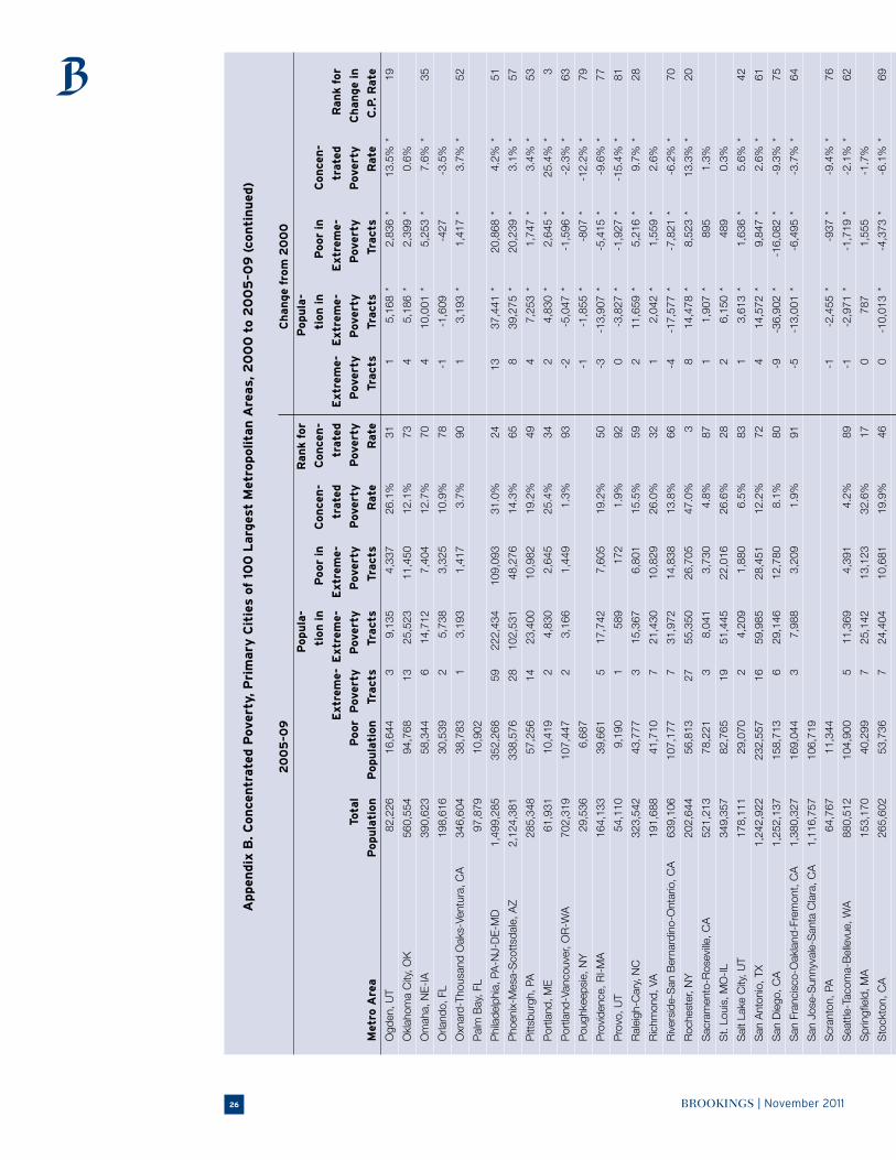
BROOKINGS | November 201126

Appen

dix

B. C

on

cen

trate

d P

over

ty, P

rim

ary

Cit

ies

of 1

00

Larg

est

Met

ropolita

n A

reas,

20

00

to 2

00

5–0

9 (

con

tin

ued

)

2

00

5–0

9

Ch

an

ge

from

20

00

Popu

la-

Ran

k fo

r

Popu

la-

ti

on

in

P

oor

in

Con

cen

- C

on

cen

-

tion

in

Poor

in

Con

cen

-

E

xtr

eme-

Extr

eme-

E

xtr

eme-

tr

ate

d

trate

d

Extr

eme-

E

xtr

eme-

E

xtr

eme-

trate

d

R

an

k fo

r

Tota

l P

oor

Pov

erty

P

over

ty

Pov

erty

P

over

ty

Pov

erty

P

over

ty

Pov

erty

Pov

erty

P

over

ty

Ch

an

ge

in

M

etro

Are

a

Popu

lati

on

P

opu

lati

on

Tr

act

s Tr

act

s Tr

act

s R

ate

R

ate

Tr

act

s Tr

act

s

Tract

s

Rate

C.P

. R

ate

Ogd

en, U

T 8

2,22

6

16,

644

3

9

,135

4

,337

26

.1%

3

1

1 5,

168

* 2,

836

* 13

.5%

*

19

Okl

ahom

a C

ity, O

K

560

,554

9

4,76

8

13

2

5,52

3

11,

450

12

.1%

7

3

4 5,

186

* 2,

399

* 0.

6%

Om

aha,

NE

-IA

3

90,6

23

58,

344

6

1

4,71

2

7,4

04

12.7

%

70

4

10,0

01 *

5,

253

* 7.

6% *

35

Orla

ndo,

FL

198

,616

3

0,53

9

2

5,7

38

3,3

25

10.9

%

78

-1

-1

,609

-4

27

-3.5

%

Oxn

ard-

Thou

sand

Oak

s-Ve

ntur

a, C

A

346

,604

3

8,78

3

1

3,1

93

1,4

17

3.7%

9

0

1 3,

193

* 1,

417

* 3.

7% *

52

Pal

m B

ay, F

L 9

7,87

9

10,

902

Phi

lade

lphi

a, P

A-N

J-D

E-M

D

1,4

99,2

85

352

,268

5

9

222

,434

1

09,0

93

31.0

%

24

13

37

,441

*

20,8

68 *

4.

2% *

51

Pho

enix

-Mes

a-S

cott

sdal

e, A

Z 2

,124

,381

3

38,5

76

28

1

02,5

31

48,

276

14

.3%

6

5

8 39

,275

*

20,2

39 *

3.

1% *

57

Pitt

sbur

gh, P

A

285

,348

5

7,25

6

14

2

3,40

0

10,

982

19

.2%

4

9

4 7,

253

* 1,

747

* 3.

4% *

53

Por

tland

, ME

6

1,93

1

10,

419

2

4

,830

2

,645

25

.4%

3

4

2 4,

830

* 2,

645

* 25

.4%

*

3

Por

tland

-Van

couv

er, O

R-W

A

702

,319

1

07,4

47

2

3,1

66

1,4

49

1.3%

9

3

-2

-5,0

47 *

-1

,596

*

-2.3

% *

63

Pou

ghke

epsi

e, N

Y

29,

536

6

,687

-1

-1,8

55 *

-8

07 *

-1

2.2%

*

79

Pro

vide

nce,

RI-

MA

1

64,1

33

39,

661

5

1

7,74

2

7,6

05

19.2

%

50

-3

-1

3,90

7 *

-5,4

15 *

-9

.6%

*

77

Pro

vo, U

T 5

4,11

0

9,1

90

1

589

1

72

1.9%

9

2

0 -3

,827

*

-1,9

27 *

-1

5.4%

*

81

Ral

eigh

-Car

y, N

C

323

,542

4

3,77

7

3

15,

367

6

,801

15

.5%

5

9

2 11

,659

*

5,21

6 *

9.7%

*

28

Ric

hmon

d, V

A

191

,688

4

1,71

0

7

21,

430

1

0,82

9

26.0

%

32

1

2,04

2 *

1,55

9 *

2.6%

Riv

ersi

de-S

an B

erna

rdin

o-O

ntar

io, C

A

639

,106

1

07,1

77

7

31,

972

1

4,83

8

13.8

%

66

-4

-1

7,57

7 *

-7,8

21 *

-6

.2%

*

70

Roc

hest

er, N

Y

202

,644

5

6,81

3

27

5

5,35

0

26,

705

47

.0%

3

8

14,4

78 *

8,

523

* 13

.3%

*

20

Sac

ram

ento

-Ros

eville

, CA

5

21,2

13

78,

221

3

8

,041

3

,730

4.

8%

87

1

1,90

7 *

895

1.

3%

St.

Loui

s, M

O-I

L 3

49,3

57

82,

765

1

9

51,

445

2

2,01

6

26.6

%

28

2

6,15

0 *

489

0.

3%

Sal

t Lak

e C

ity, U

T 1

78,1

11

29,

070

2

4

,209

1

,880

6.

5%

83

1

3,61

3 *

1,63

6 *

5.6%

*

42

San

Ant

onio

, TX

1,2

42,9

22

232

,557

1

6

59,

985

2

8,45

1

12.2

%

72

4

14,5

72 *

9,

847

* 2.

6% *

61

San

Die

go, C

A

1,2

52,1

37

158

,713

6

2

9,14

6

12,

780

8.

1%

80

-9

-3

6,90

2 *

-16,

082

* -9

.3%

*

75

San

Fra

ncis

co-O

akla

nd-F

rem

ont,

CA

1

,380

,327

1

69,0

44

3

7,9

88

3,2

09

1.9%

9

1

-5

-13,

001

* -6

,495

*

-3.7

% *

64

San

Jos

e-S

unny

vale

-San

ta C

lara

, CA

1

,116

,757

1

06,7

19

Scr

anto

n, P

A

64,

767

1

1,34

4

-1

-2

,455

*

-937

*

-9.4

% *

76

Sea

ttle

-Tac

oma-

Bel

levu

e, W

A

880

,512

1

04,9

00

5

11,

369

4

,391

4.

2%

89

-1

-2

,971

*

-1,7

19 *

-2

.1%

*

62

Spr

ingfi

eld

, MA

1

53,1

70

40,

299

7

2

5,14

2

13,

123

32

.6%

1

7

0 78

7

1,55

5

-1.7

%

Sto

ckto

n, C

A

265

,602

5

3,73

6

7

24,

404

1

0,68

1

19.9

%

46

0

-10,

013

* -4

,373

*

-6.1

% *

69

BROOKINGS | November 2011 27

Syr

acus

e, N

Y

127

,701

3

5,91

9

16

3

5,41

3

16,

419

45

.7%

4

7

13,1

35 *

6,

152

* 14

.8%

*

16

Tam

pa-S

t. P

eter

sbur

g-C

lear

wat

er, F

L 6

21,7

14

103

,855

1

1

31,

897

1

5,12

1

14.6

%

64

0

2,27

4

599

-0

.9%

Tole

do, O

H

313

,643

6

9,03

4

21

4

1,60

8

21,

119

30

.6%

2

5

14

28,7

73 *

14

,976

*

19.4

% *

10

Tucs

on, A

Z 5

02,1

49

100

,240

6

3

5,14

3

15,

697

15

.7%

5

8

4 32

,397

*

14,4

79 *

14

.2%

*

17

Tuls

a, O

K

374

,609

6

8,21

9

8

20,

892

1

0,11

1

14.8

%

61

2

6,52

5 *

4,05

7 *

3.3%

*

54

Virg

inia

Bea

ch-N

orfo

lk-N

ewpo

rt N

ews,

VA

-NC

8

57,9

77

89,

572

8

2

0,96

5

10,

295

11

.5%

7

5

-4

-13,

246

* -7

,264

*

-8.1

% *

73

Was

hing

ton-

Arli

ngto

n-A

lexa

ndria

,

D

C-V

A-M

D-W

V

932

,350

1

26,3

22

17

5

0,63

2

22,

164

17

.5%

5

3

-3

-6,2

56 *

-2

,578

*

-0.9

%

Wic

hita

, KS

3

33,4

94

51,

993

6

1

4,49

4

6,1

73

11.9

%

74

4

9,00

2 *

3,78

6 *

5.6%

*

41

Wor

cest

er, M

A

166

,513

2

7,92

2

3

10,

769

5

,299

19

.0%

5

1

1 3,

552

* 1,

959

* 7.

5% *

36

Youn

gsto

wn,

OH

-PA

7

2,88

0

21,

794

1

2

23,

226

1

0,82

5

49.7

%

1

7 16

,716

*

8,26

4 *

36.3

% *

2

*Ch

ang

e is

sig

nifi

can

t at

th

e 9

0 p

erce

nt

confi

den

ce le

vel.

S

ou

rce:

Bro

oki

ng

s In

stit

uti

on

an

lays

is o

f d

ecen

nia

l cen

sus

and

AC

S d

ata

BROOKINGS | November 201128

Appen

dix

C. C

on

cen

trate

d P

over

ty, S

ubu

rbs

of 1

00

Larg

est

Met

ropolita

n A

reas,

20

00

to 2

00

5–0

9

2

00

5–0

9

Ch

an

ge

from

20

00

Popu

la-

Ran

k fo

r

Popu

la-

ti

on

in

P

oor

in C

on

cen

- C

on

cen

-

tion

in

Poor

in

Con

cen

-

E

xtr

eme-

Extr

eme-

E

xtr

eme-

tr

ate

d

trate

d

Extr

eme-

E

xtr

eme-

E

xtr

eme-

trate

d

R

an

k fo

r

Tota

l P

oor

Pov

erty

P

over

ty

Pov

erty

Pov

erty

P

over

ty

Pov

erty

P

over

ty

P

over

ty

Pov

erty

C

han

ge

in

M

etro

Are

a

Popu

lati

on

P

opu

lati

on

Tr

act

s Tr

act

s Tr

act

s R

ate

R

ate

Tr

act

s Tr

act

s

Tract

s

Rate

C.P

. R

ate

100

Larg

est

Met

ro A

reas

13

5,65

4,15

2

12,6

96,6

09

344

1,

240,

791

57

0,72

9

4.5%

122

33

5,83

6 *

164,

874

* 0.

5% *

Akr

on, O

H

479

,805

4

1,15

0

1

3,9

08

1,7

83

4.3%

3

6

1 3,

908

* 1,

783

* 4.

3% *

15

Alb

any,

NY

7

45,0

15

62,

149

4

9

,412

4

,451

7.

2%

20

1

3,01

6 *

1,67

3 *

2.0%

*

34

Alb

uque

rque

, NM

3

36,8

62

48,

349

3

7

,319

3

,117

6.

4%

23

2

4,36

1 *

1,20

2 *

1.7%

*

37

Alle

ntow

n, P

A-N

J 6

93,5

69

46,

292

2

7

,350

2

,844

6.

1%

24

1

2,92

2 *

867

* 1.

1%

Atla

nta,

GA

4

,731

,351

5

16,2

89

5

14,

275

6

,482

1.

3%

63

1

-1,8

84 *

-3

78

-1.0

% *

56

Aug

usta

-Ric

hmon

d C

ount

y, G

A-S

C

330

,562

4

5,30

0

2

9,8

76

3,9

94

8.8%

1

5

1 5,

324

* 1,

835

* 3.

1% *

27

Aus

tin, T

X 9

28,5

74

82,

696

2

1

5,59

4

7,5

74

9.2%

1

4

1 5,

446

* 3,

594

* 0.

7%

Bak

ersfi

eld

, CA

5

15,7

56

101

,190

4

1

8,33

3

8,6

68

8.6%

1

7

-2

-12,

203

* -4

,363

*

-6.4

% *

68

Bal

timor

e, M

D

2,0

21,1

40

119

,414

Bat

on R

ouge

, LA

5

43,2

61

67,

814

2

1

0,77

0

4,7

64

7.0%

2

1

2 1

0,77

0 *

4,7

64 *

7.

0% *

5

Birm

ingh

am, A

L 9

05,3

28

90,

075

1

4

,355

1

,978

2.

2%

53

0

-727

*

-657

*

-1.0

% *

57

Boi

se C

ity, I

D

417

,401

4

6,88

1

2

4,7

31

1,6

87

3.6%

4

1

2 4,

731

* 1,

687

* 3.

6% *

21

Bos

ton-

Cam

brid

ge, M

A-N

H

3,7

42,8

08

271

,970

7

1

7,89

0

8,1

14

3.0%

4

7

3 10

,755

*

4,59

4 *

1.5%

*

40

Bra

dent

on, F

L 6

42,7

19

66,

140

Brid

gepo

rt-S

tam

ford

, CT

627

,752

2

6,87

1

1

3,1

03

1,3

51

5.0%

3

4

1 3,

103

* 1,

351

* 5.

0% *

13

Buf

falo

, NY

8

50,2

75

73,

599

4

7

,345

3

,627

4.

9%

35

2

3,52

7 *

1,75

8 *

1.8%

*

36

Cap

e C

oral

, FL

425

,396

4

6,85

5

1

4,5

79

2,5

72

5.5%

3

0

0 -2

64

-241

-2

.5%

*

62

Cha

rlest

on, S

C

514

,336

6

7,26

2

4

9,1

70

4,0

21

6.0%

2

8

0 -3

,432

*

-1,0

60 *

-3

.2%

*

63

Cha

rlott

e, N

C-S

C

1,1

21,5

09

119

,304

1

2

,141

8

89

0.7%

6

8

1 2,

141

* 88

9 *

0.7%

*

48

Cha

ttan

ooga

, TN

-GA

3

39,8

80

38,

011

Chi

cago

-Nap

ervi

lle-J

olie

t, IL

-IN

-WI

6,3

30,3

87

508

,942

2

0

36,

947

1

8,17

2

3.6%

4

2

11

18,1

32 *

10

,010

*

1.3%

*

42

Cin

cinn

ati,

OH

-KY-

IN

1,7

88,9

46

162

,098

1

0

22,

731

9

,928

6.

1%

26

7

17,2

29 *

7,

481

* 3.

9% *

17

Cle

vela

nd, O

H

1,6

54,6

99

150

,868

1

2

24,

297

1

2,13

5

8.0%

1

8

12

24,2

97 *

12

,135

*

8.0%

*

4

Col

orad

o S

prin

gs, C

O

220

,185

1

6,64

0

Col

umbi

a, S

C

621

,294

7

4,32

5

2

5,5

88

2,4

10

3.2%

4

4

1 2,

675

* 1,

229

* 1.

3% *

43

Col

umbu

s, O

H

1,0

81,4

70

86,

902

1

9

11

531

0.

6%

72

1

911

* 53

1 *

0.6%

*

50

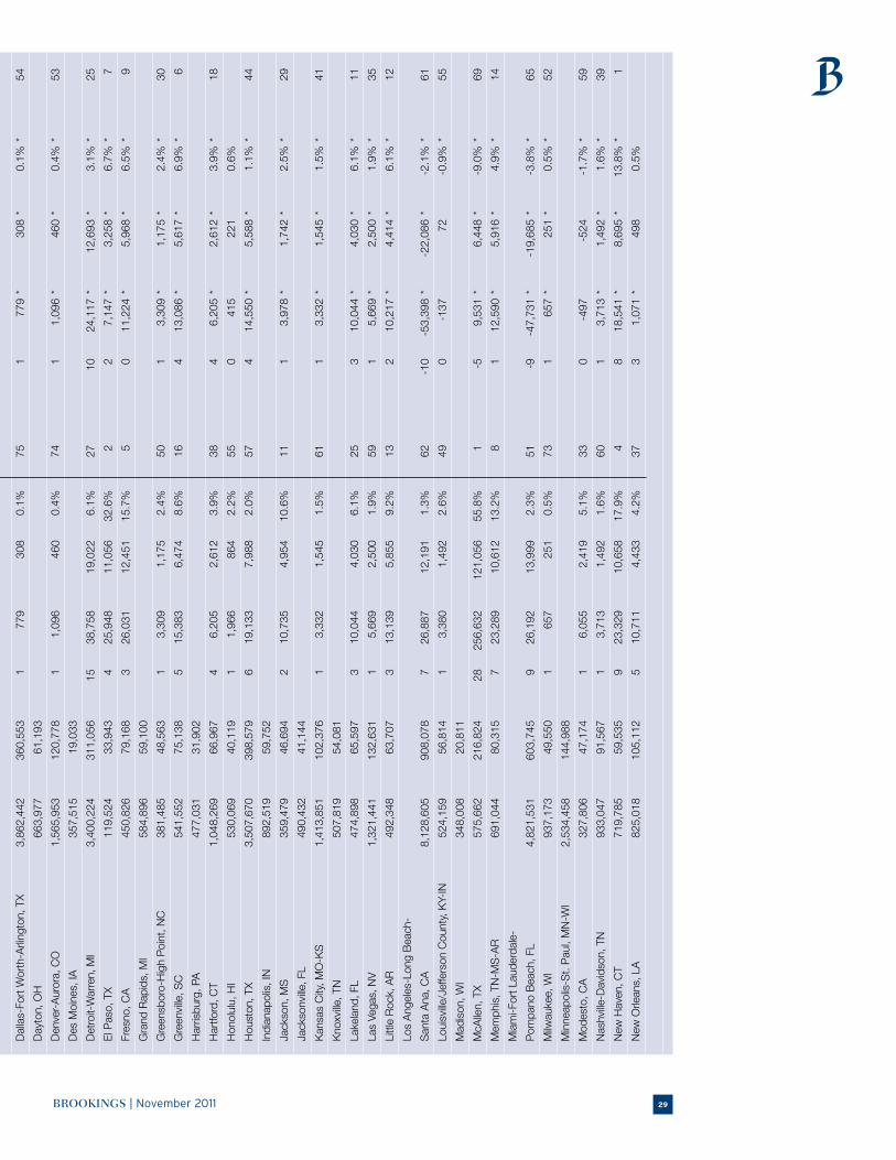
BROOKINGS | November 2011 29

Dal

las-

Fort

Wor

th-A

rling

ton,

TX

3,8

62,4

42

360

,553

1

7

79

308

0.

1%

75

1

779

* 30

8 *

0.1%

*

54

Day

ton,

OH

6

63,9

77

61,

193

Den

ver-

Aur

ora,

CO

1

,565

,953

1

20,7

78

1

1,0

96

460

0.

4%

74

1

1,09

6 *

460

* 0.

4% *

53

Des

Moi

nes,

IA

357

,515

1

9,03

3

Det

roit-

War

ren,

MI

3,4

00,2

24

311

,056

1

5

38,

758

1

9,02

2

6.1%

2

7

10

24,1

17 *

12

,693

*

3.1%

*

25

El P

aso,

TX

119

,524

3

3,94

3

4

25,

948

1

1,05

6

32.6

%

2

2 7,

147

* 3,

258

* 6.

7% *

7

Fres

no, C

A

450

,826

7

9,16

8

3

26,

031

1

2,45

1

15.7

%

5

0 11

,224

*

5,96

8 *

6.5%

*

9

Gra

nd R

apid

s, M

I 5

84,8

96

59,

100

Gre

ensb

oro-

Hig

h P

oint

, NC

3

81,4

85

48,

563

1

3

,309

1

,175

2.

4%

50

1

3,30

9 *

1,17

5 *

2.4%

*

30

Gre

envi

lle, S

C

541

,552

7

5,13

8

5

15,

383

6

,474

8.

6%

16

4

13,0

86 *

5,

617

* 6.

9% *

6

Har

risbu

rg, P

A

477

,031

3

1,90

2

Har

tford

, CT

1,0

48,2

69

66,

967

4

6

,205

2

,612

3.

9%

38

4

6,20

5 *

2,61

2 *

3.9%

*

18

Hon

olul

u, H

I 5

30,0

69

40,

119

1

1

,966

8

64

2.2%

5

5

0 41

5

221

0.

6%

Hou

ston

, TX

3,5

07,6

70

398

,579

6

1

9,13

3

7,9

88

2.0%

5

7

4 14

,550

*

5,58

8 *

1.1%

*

44

Indi

anap

olis

, IN

8

92,5

19

59,

752

Jack

son,

MS

3

59,4

79

46,

694

2

1

0,73

5

4,9

54

10.6

%

11

1

3,97

8 *

1,74

2 *

2.5%

*

29

Jack

sonv

ille, F

L 4

90,4

32

41,

144

Kan

sas

City

, MO

-KS

1

,413

,851

1

02,3

76

1

3,3

32

1,5

45

1.5%

6

1

1 3,

332

* 1,

545

* 1.

5% *

41

Kno

xville

, TN

5

07,8

19

54,

081

Lake

land

, FL

474

,898

6

5,59

7

3

10,

044

4

,030

6.

1%

25

3

10,0

44 *

4,

030

* 6.

1% *

11

Las

Vega

s, N

V

1,3

21,4

41

132

,631

1

5

,669

2

,500

1.

9%

59

1

5,66

9 *

2,50

0 *

1.9%

*

35

Litt

le R

ock,

AR

4

92,3

48

63,

707

3

1

3,13

9

5,8

55

9.2%

1

3

2 10

,217

*

4,41

4 *

6.1%

*

12

Los

Ang

eles

-Lon

g B

each

-

S

anta

Ana

, CA

8

,128

,605

9

08,0

78

7

26,

887

1

2,19

1

1.3%

6

2

-10

-53,

398

* -2

2,08

6 *

-2.1

% *

61

Loui

sville

/Jef

fers

on C

ount

y, K

Y-IN

5

24,1

59

56,

814

1

3

,380

1

,492

2.

6%

49

0

-137

72

-0

.9%

*

55

Mad

ison

, WI

348

,008

2

0,81

1

McA

llen,

TX

575

,662

2

16,8

24

28

2

56,6

32

121

,056

55

.8%

1

-5

9,

531

* 6,

448

* -9

.0%

*

69

Mem

phis

, TN

-MS

-AR

6

91,0

44

80,

315

7

2

3,28

9

10,

612

13

.2%

8

1

12,5

90 *

5,

916

* 4.

9% *

14

Mia

mi-F

ort L

aude

rdal

e-

P

ompa

no B

each

, FL

4,8

21,5

31

603

,745

9

2

6,19

2

13,

999

2.

3%

51

-9

-4

7,73

1 *

-19,

685

* -3

.8%

*

65

Milw

auke

e, W

I 9

37,1

73

49,

550

1

6

57

251

0.

5%

73

1

657

* 25

1 *

0.5%

*

52

Min

neap

olis

-St.

Pau

l, M

N-W

I 2

,534

,458

1

44,9

88

Mod

esto

, CA

3

27,8

06

47,

174

1

6

,055

2

,419

5.

1%

33

0

-497

-5

24

-1.7

% *

59

Nas

hville

-Dav

idso

n, T

N

933

,047

9

1,56

7

1

3,7

13

1,4

92

1.6%

6

0

1 3,

713

* 1,

492

* 1.

6% *

39

New

Hav

en, C

T 7

19,7

85

59,

535

9

2

3,32

9

10,

658

17

.9%

4

8

18,5

41 *

8,

695

* 13

.8%

*

1

New

Orle

ans,

LA

8

25,0

18

105

,112

5

1

0,71

1

4,4

33

4.2%

3

7

3 1,

071

* 49

8

0.5%

BROOKINGS | November 201130

Appen

dix

C. C

on

cen

trate

d P

over

ty, S

ubu

rbs

of 1

00

Larg

est

Met

ropolita

n A

reas,

20

00

to 2

00

5–0

9 (

con

tin

ued

)

2

00

5–0

9

Ch

an

ge

from

20

00

Popu

la-

Ran

k fo

r

Popu

la-

ti

on

in

P

oor

in C

on

cen

- C

on

cen

-

tion

in

Poor

in

Con

cen

-

E

xtr

eme-

Extr

eme-

E

xtr

eme-

tr

ate

d

trate

d

Extr

eme-

E

xtr

eme-

E

xtr

eme-

trate

d

R

an

k fo

r

Tota

l P

oor

Pov

erty

P

over

ty

Pov

erty

Pov

erty

P

over

ty

Pov

erty

P

over

ty

P

over

ty

Pov

erty

C

han

ge

in

M

etro

Are

a

Popu

lati

on

P

opu

lati

on

Tr

act

s Tr

act

s Tr

act

s R

ate

R

ate

Tr

act

s Tr

act

s

Tract

s

Rate

C.P

. R

ate

New

Yor

k-N

orth

ern

New

Jer

sey,

N

Y-N

J-PA

1

0,29

5,12

5

733

,870

2

6

95,

122

4

2,92

7

5.8%

2

9

10

39,1

26 *

18

,022

*

2.3%

*

31

Ogd

en, U

T 4

33,3

99

24,

727

-1

-1,3

41 *

-9

46 *

-5

.1%

*

67

Okl

ahom

a C

ity, O

K

608

,707

7

2,22

0

-2

-2

,110

*

-896

*

-1.5

% *

58

Om

aha,

NE

-IA

4

37,4

37

30,

062

1

1

,699

6

80

2.3%

5

2

1 1,

699

* 68

0 *

2.3%

*

32

Orla

ndo,

FL

1,8

15,1

62

200

,585

2

8

,784

4

,366

2.

2%

54

1

4,13

7 *

2,02

2 *

0.5%

*

51

Oxn

ard-

Thou

sand

Oak

s-Ve

ntur

a, C

A

445

,709

3

2,01

8

Pal

m B

ay, F

L 4

34,8

18

40,

777

4

1

3,73

9

5,8

59

14.4

%

7

3 10

,209

*

4,34

0 *

10.2

% *

3

Phi

lade

lphi

a, P

A-N

J-D

E-M

D

4,3

54,2

33

311

,061

2

3

69,

918

3

3,01

7

10.6

%

10

8

24,6

33 *

14

,804

*

3.6%

*

22

Pho

enix

-Mes

a-S

cott

sdal

e, A

Z 2

,012

,111

2

05,3

09

6

25,

972

1

0,81

9

5.3%

3

2

2 14

,008

*

4,87

1 *

0.5%

Pitt

sbur

gh, P

A

2,0

37,5

63

207

,287

8

1

4,74

4

6,3

42

3.1%

4

6

1 -1

70

187

-0

.2%

Por

tland

, ME

4

52,1

13

37,

399

Por

tland

-Van

couv

er, O

R-W

A

1,4

60,7

78

142

,043

1

4

,486

1

,248

0.

9%

66

1

4,48

6 *

1,24

8 *

0.9%

*

46

Pou

ghke

epsi

e, N

Y

625

,618

5

7,37

3

3

26,

569

1

7,32

6

30.2

%

3

1 12

,202

*

9,14

1 *

13.1

% *

2

Pro

vide

nce,

RI-

MA

1

,417

,389

1

34,0

53

6

15,

011

7

,206

5.

4%

31

4

10,6

02 *

5,

285

* 3.

8% *

19

Pro

vo, U

T 4

06,8

63

29,

973

1

5

01

202

0.

7%

70

1

501

* 20

2

0.7%

Ral

eigh

-Car

y, N

C

711

,051

6

1,55

7

Ric

hmon

d, V

A

1,0

04,5

44

79,

801

3

1

0,68

2

2,7

90

3.5%

4

3

3 10

,682

*

2,79

0 *

3.5%

*

23

Riv

ersi

de-S

an B

erna

rdin

o-O

ntar

io, C

A

3,3

78,3

02

415

,414

3

1

0,96

0

5,1

90

1.2%

6

4

-3

-16,

978

* -6

,679

*

-2.0

% *

60

Roc

hest

er, N

Y

809

,089

6

4,43

0

Sac

ram

ento

-Ros

eville

, CA

1

,539

,927

1

62,0

80

1

7,7

39

3,1

48

1.9%

5

8

-3

-12,

225

* -4

,536

*

-3.6

% *

64

St.

Loui

s, M

O-I

L 2

,434

,321

2

30,8

86

12

3

8,47

2

17,

851

7.

7%

19

6

18,3

39 *

7,

942

* 2.

3% *

33

Sal

t Lak

e C

ity, U

T 9

11,3

65

68,

332

San

Ant

onio

, TX

770

,428

7

7,84

0

1

3,8

15

1,6

24

2.1%

5

6

0 3,

100

* 1,

397

* 1.

7% *

38

San

Die

go, C

A

1,7

08,0

17

171

,912

2

5

,314

1

,078

0.

6%

71

1

3,67

5 *

441

0.

2%

San

Fra

ncis

co-O

akla

nd-F

rem

ont,

CA

2

,808

,873

2

23,0

23

2

3,7

78

1,5

31

0.7%

6

9

2 3,

778

* 1,

531

* 0.

7% *

49

San

Jos

e-S

unny

vale

-San

ta C

lara

, CA

6

46,9

41

42,

439

Scr

anto

n, P

A

476

,654

5

5,35

3

2

4,9

41

2,0

37

3.7%

4

0

2 4,

941

* 2,

037

* 3.

7% *

20

Sea

ttle

-Tac

oma-

Bel

levu

e, W

A

2,4

02,1

54

207

,501

2

5

,795

2

,203

1.

1%

65

2

5,79

5 *

2,20

3 *

1.1%

*

45

BROOKINGS | November 2011 31

Spr

ingfi

eld

, MA

5

20,8

01

58,

565

5

1

6,31

1

8,4

30

14.4

%

6

1 5,

738

* 3,

296

* 4.

2% *

16

Sto

ckto

n, C

A

399

,039

4

5,66

0

Syr

acus

e, N

Y

494

,112

4

2,82

3

1

3,1

53

1,2

57

2.9%

4

8

1 3,

153

* 1,

257

* 2.

9% *

28

Tam

pa-S

t. P

eter

sbur

g-C

lear

wat

er, F

L 2

,075

,179

2

24,8

37

2

17,

161

6

,928

3.

1%

45

2

17,1

61 *

6,

928

* 3.

1% *

26

Tole

do, O

H

345

,371

2

9,28

1

1

4,4

75

1,9

42

6.6%

2

2

1 4,

475

* 1,

942

* 6.

6% *

8

Tucs

on, A

Z 4

80,6

72

51,

143

4

1

2,41

0

6,1

32

12.0

%

9

-1

-3,8

87 *

-1

,570

*

-9.3

% *

70

Tuls

a, O

K

523

,540

5

6,95

3

1

1,2

54

475

0.

8%

67

1

1,25

4 *

475

* 0.

8% *

47

Virg

inia

Bea

ch-N

orfo

lk-N

ewpo

rt N

ews,

VA

-NC

7

96,1

64

71,

343

-3

-6,3

88 *

-2

,970

*

-4.4

% *

66

Was

hing

ton-

Arli

ngto

n-A

lexa

ndria

,

D

C-V

A-M

D-W

V

4,3

87,6

64

241

,977

Wic

hita

, KS

2

62,7

21

19,

986

Wor

cest

er, M

A

617

,223

4

1,48

0

3

2,5

26

1,5

44

3.7%

3

9

2 1,

887

* 1,

412

* 3.

4% *

24

Youn

gsto

wn,

OH

-PA

4

92,1

79

59,

263

7

1

2,46

3

5,5

88

9.4%

1

2

4 9,

108

* 4,

126

* 6.

4% *

10

*Ch

ang

e is

sig

nifi

can

t at

th

e 9

0 p

erce

nt

confi

den

ce le

vel.

S

ou

rce:

Bro

oki

ng

s In

stit

uti

on

an

lays

is o

f d

ecen

nia

l cen

sus

and

AC

S d

ata

BROOKINGS | November 201132

Endnotes

1. Alan Berube and Elizabeth Kneebone, “Parsing U.S.

Poverty at the Metropolitan Level” Brookings Up Front

Blog, http://www.brookings.edu/opinions/2011/0922_

metro_poverty_berube_kneebone.aspx, posted 9/22/2011.

2. Elizabeth Kneebone and Alan Berube, “Reversal of

Fortune: A New Look at Concentrated Poverty in the

2000s” (Washington: Brookings Institution, 2008).

3. Paul Jargowsky, “Stunning Progress, Hidden Problems“

(Washington: Brookings institution, 2003); Community

Affairs Offi ces of the Federal Reserve System and the

Brookings Institution, “The Enduring Challenge of

Concentrated Poverty in America: Case Studies from

Communities Across the U.S.” (Washington: 2008).

4. Paul Jargowsky, Poverty and Place: Ghettos, Barrios, and

the American City (New York: Russell Sage Foundation,

1997); Paul Jargowsky, “Stunning Progress, Hidden

Problems”.

5. Kneebone and Berube, “Reversal of Fortune”. See also,

Rolf Pendall and others, “A Lost Decade: Neighborhood

Poverty and the Urban Crisis of the 2000s” (Washington:

Joint Center for Political and Economic Studies, 2011).

6. See, e.g., Paul Jargowsky and Mary Jo Bane, “Ghetto

Poverty in the United States” in C. Jenks and P.

Peterson, eds., The Urban Underclass. (Washington:

Brookings Institution, 1991); Sheldon H. Danziger and

Peter Gottschalk, “Earnings Inequality, the Spatial

Concentration of Poverty, and the Underclass,” American

Economic Review 77 (1987); Jargowsky and Mary Jo

Bane, “Ghetto Poverty: Basic Questions” in L. E. Lynn and

M. G. H. McGeary, eds., Inner-City Poverty in the United

States (Washington: National Academy Press, 1991); John

D. Kasarda, “Inner-City Poverty and Economic Access”

in J. Sommer and D. A. Hicks, eds., Rediscovering Urban

America: Perspectives on the 1980s (U.S. Department

of Housing and Urban Development, 1993); G. Thomas

Kingsley and Kathryn Pettit, “Severe Distress and

Concentrated Poverty: Trends for Neighborhoods

in Casey Cities and the Nation” (Washington: Urban

Institute, 2003).

7. For a more detailed discussion of potential bias that can

result for using standardized tract boundaries across

years, see Jargowsky, “Stunning Progress, Hidden

Problems”.

8. For a more detailed discussion of geography types,

see Brookings Metropolitan Policy Program, “State

of Metropolitan America: On the Front Lines of

Demographic Transformation” (Washington: 2010).

9. See e.g., National Academy of Sciences, Measuring

Poverty: A New Approach (Washington: National

Academy Press, 1995). The Census Bureau plans to begin

releasing a supplemental poverty measure in 2012 that

takes into account recommendations from the 1995 NAS

study; however, because the estimates will be based on

the Current Population Survey data, the sample size will

not be suffi cient to report estimates for sub-state geog-

raphies.

10. We exclude tracts where at least 50 percent of residents

are enrolled in college or graduate school, as these indi-

viduals likely have only temporarily low incomes. We also

exclude tracts with small populations (i.e., 500 people or

less).

11. Jargowsky, “Stunning Progress, Hidden Problems”.

12. In addition, as Paul Jargowsky recently pointed out in a

presentation at Johns Hopkins University (9/19/2011), a

region could have the same number of extreme-poverty

tracts in each month for 60 months, but the exact tracts

that are high poverty could change over time, due to fac-

tors like gentrifi cation or the demolition of housing units.

It would then be possible, after pooling 60 months of

data, that zero tracts show up as extreme poverty in the

2005–09 estimates, thereby understating concentrated

poverty in the region.

13. The model produces an R-squared of .541.

14. Jargowsky, Poverty and Place.

15. For an analysis of concentrated poverty trends since

1970, see Paul Jargowsky, Poverty and Place; Berube and

Katz, “Katrina’s Window”.

16. Jargowsky, “Stunning Progress, Hidden Problems”.

17. Jargowsky, “Stunning Progress, Hidden Problems”.

18. New Orleans’ signifi cant decline in concentrated poverty

was largely the result of natural disasters, with the evacu-

ations and destruction following Hurricanes Katrina and

Rita driving this region’s trend.

BROOKINGS | November 2011 33

19. Berube and Kneebone, “Parsing U.S. Poverty at the

Metropolitan Level.”

20. Elizabeth Kneebone and Alan Berube, “The Rapid Growth

of the Suburban Poor” The Atlantic Cities, http://www.

theatlanticcities.com/jobs-and-economy/2011/09/rapid-

growth-suburban-poor/190/, posted 9/23/2011.

21. Kneebone and Garr, “The Suburbanization of Poverty”.

22. George C. Galster, “The Mechanism(s) of Neighborhood

Effects: Theory, Evidence, and Policy Implications”

Presentation at the ESRC Seminar, St. Andrews

University, Scotland, UK, 4–5 February 2010.

23. Jargwosky, “Stunning Progress, Hidden Problems”.

24. Erol Ricketts and Isabel Sawhill, “Defi ning and Measuring

the Underclass” Journal of Policy Analysis and

Management Vol. 7 (2) (1988: 316-325) pp.321; See also,

Isabel Sawhill and Paul Jargowsky, “The Decline of the

Underclass” (Washington: Brookings Institution, 2006).

25. Ricketts and Sawhill, “Defi ning and Measuring the

Underclass” pp. 322-323.

26. Recent research has also found that the share of all

whites, of all blacks, and of all Latinos living in high-

poverty tracts largely stayed the same over the decade,

meaning the shifts in the racial and ethnic composition

of these neighborhoods was driven by changes in the

composition of the larger population. See Pendall and

others, “The Lost Decade.”

27. Steven Raphael and Michael Stoll, “Job Sprawl and the

Suburbanization of Poverty” (Washington: Brookings

Institution, 2010); Kenya Covington, Lance Freeman, and

Michael Stoll, “The Suburbanization of Housing Choice

Voucher Recipients” (Washington: Brookings Institution,

2011).

BROOKINGS | November 201134

AcknowledgementsThe authors thank Paul Jargowsky, Jens Ludwig, and Rolf Pendall for their comments on a draft of this paper, and Chris Ingraham for his assistance on graphics.

The Metropolitan Policy Program at Brookings thanks the Ford Foundation for its generous sup-port of the program’s research on city and suburban poverty and opportunity, the Annie E. CaseyFoundation for its support of the program’s research on low-income working families, and theJohn D. and Catherine T. MacArthur Foundation, the George Gund Foundation, the F.B. HeronFoundation, and the Heinz Endowments for their general support of the program, as well as themembers of the Metropolitan Leadership Council.

For More InformationElizabeth KneeboneSenior Research AssociateMetropolitan Policy Program at Brookings202.797.6108ekneebone@brookings.edu

Carey NadeauSenior Research AssistantMetropolitan Policy Program at Brookings202.797.6221 cnadeau@brookings.edu

Alan BerubeSenior Fellow and Research DirectorMetropolitan Policy Program at Brookings202.797.6075 aberube@brookings.edu

For General InformationMetropolitan Policy Program at Brookings202.797.6139www.brookings.edu/metro

The Brookings Institution is a private non-profi t organization. Its mission is to conduct high quality, independent research and, based on that research, to provide innovative, practical recommen dations for policymakers and the public. The conclusions and recommendations of any Brookings publication are solely those of its author(s), and do not refl ect the views of the Institution, its management, or its other scholars.

Brookings recognizes that the value it provides to any supporter is in its absolute commitment to quality, independence and impact. Activities supported by its donors refl ect this commitment and the analysis and recommendations are not determined by any donation.

1775 Massachusetts Avenue, NW Washington D.C. 20036-2188telephone 202.797.6000fax 202.797.6004web site www.brookings.edu

telephone 202.797.6139 fax 202.797.2965web site www.brookings.edu/metro

BROOKINGS

About the Metropolitan Policy Program at BrookingsCreated in 1996, the Metropolitan Policy Program provides decisionmakers with cutting-edge research and policy ideas for improving the health and prosperity of metropolitan areas including their component cities, suburbs, and rural areas. To learn more visit www.brookings.edu/metro.

About the Brookings Metropolitan Opportunity SeriesLaunched in 2009, the Metropolitan Opportunity Series docu-ments the changing geography of poverty and opportunity in metropolitan America, analyzes its drivers and implications, and offers policy recommendations to enhance the well-being of lower-income families and communities in both cities and suburbs. This study and other publica tions, speeches, presenta-tions, and commentary in the series are available at: www.brookings.edu/metro/Metropolitan-Opportunity.aspx

In the Series■ Missed Opportunity: Transit and Jobs in Metropolitan America■ Job Sprawl and the Suburbanization of Poverty

Forthcoming■ Affordable Housing and Access to Transit■ Job Sprawl in the 2000s (Before and After the ‘Great Recession’)