Metropolitan Business Cycle Analysis for Lubbock

University of Texas at El PasoDigitalCommons@UTEP

Departmental Papers (E & F) Department of Economics and Finance

3-2017

Metropolitan Business Cycle Analysis for LubbockThomas M. Fullerton Jr.University of Texas at El Paso, [email protected]

Macie Z. SubiaUniversity of Texas at El Paso, [email protected]

Follow this and additional works at: https://digitalcommons.utep.edu/econ_papers

Part of the Regional Economics CommonsComments:In Journal of Economics and Political Economy, Volume 4, Issue 1, March 2017

This Article is brought to you for free and open access by the Department of Economics and Finance at DigitalCommons@UTEP. It has been acceptedfor inclusion in Departmental Papers (E & F) by an authorized administrator of DigitalCommons@UTEP. For more information, please [email protected].

Recommended CitationFullerton, Thomas M. Jr. and Subia, Macie Z., "Metropolitan Business Cycle Analysis for Lubbock" (2017). Departmental Papers (E &F). 95.https://digitalcommons.utep.edu/econ_papers/95

https://digitalcommons.utep.edu?utm_source=digitalcommons.utep.edu%2Fecon_papers%2F95&utm_medium=PDF&utm_campaign=PDFCoverPages

https://digitalcommons.utep.edu/econ_papers?utm_source=digitalcommons.utep.edu%2Fecon_papers%2F95&utm_medium=PDF&utm_campaign=PDFCoverPages

https://digitalcommons.utep.edu/econ_finance?utm_source=digitalcommons.utep.edu%2Fecon_papers%2F95&utm_medium=PDF&utm_campaign=PDFCoverPages

https://digitalcommons.utep.edu/econ_papers?utm_source=digitalcommons.utep.edu%2Fecon_papers%2F95&utm_medium=PDF&utm_campaign=PDFCoverPages

http://network.bepress.com/hgg/discipline/1307?utm_source=digitalcommons.utep.edu%2Fecon_papers%2F95&utm_medium=PDF&utm_campaign=PDFCoverPages

https://digitalcommons.utep.edu/econ_papers/95?utm_source=digitalcommons.utep.edu%2Fecon_papers%2F95&utm_medium=PDF&utm_campaign=PDFCoverPages

mailto:[email protected]

Journal of

Economics and Political Economy www.kspjournals.org

Volume 4 March 2017 Issue 1

Metropolitan Business Cycle Analysis for Lubbock

By Thomas M. FULLERTON a† & Macie Z. SUBIAab

Abstract. This study develops a business cycle index (BCI) for Lubbock Metropolitan Statistical Area (MSA). The Stock & Watson (1989; 1991; 1993) methodology is used to develop the BCI and assumes that the co-movements of key economic indicators have a single underlying, unobservable factor. This factor is extracted from the indicators and used to calculate an index that represents economic conditions through an econometric approach. The model uses the Kalman filter smoothing approach which smooths across variables and over time. This results in an index that is smoother with less pronounced expansions and recessions. Indicator series used for the study are: establishment employment, unemployment, real retail sales and real wages that begin in 1990 and include complete data through the end of 2015. Results indicate that the Lubbock business cycle has peaks and troughs that occur later than those for the national economy. Keywords. Regional Economics; Business Cycles; Economic Indicators. JEL. R15, E32.

1. Introduction he economic performance of Lubbock is generally difficult to assess. Although some monthly labor market and real estate data exist, there is no overall gauge of current economic activity (LEDA, 2009). One means for

doing so is provided by a business cycle index. A business cycle index (BCI) is designed using a set of economic indicators that define the state of an economy over time (Cañas, Coronado, & Lopez, 2005). While BCIs are useful tools, relatively few exist for metropolitan economies in the United States.

The objective of this study is to develop a BCI for Lubbock. To achieve that goal, the Stock & Watson (1998; 1999) methodology is used to create the index. Indicators utilized for this purpose include establishment employment, the unemployment rate, real wages, and real retail sales. The empirical method extracts from each series information relevant to the current state of the Lubbock economy and combines this information into an index that reflect metropolitan business cycle conditions (Cañas, Gilmer, & Phillips, 2003).

Remaining sections of the study are as follows. A brief overview of prior research on regional business cycle indices is provided in the next section. Data and methodology are reviewed next. Empirical results are then discussed. The final section includes a summary and closing statements. aa† Department of Economics &Finance, University of Texas at El Paso, El Paso, TX 79968-0543,

USA.

. 915-747-7747 . [email protected]

b Department of Economics &Finance, University of Texas at El Paso, El Paso, TX 79968-0543, USA.

. 915-227-9935 . [email protected]

T

Journal of Economics and Political Economy

JEPE, 4(1), T. Fullerton, & M.Z. Subia, p.33-52.

34

34

2. Literature Review The need to measure overall economic activity, and the lack of consensus on the

appropriate method to do so, has led to a great deal of research on BCIs. Beginning in 1930, the National Bureau of Economic Research (NBER) started publishing empirical business cycle studies (Burns & Mitchell, 1946). That approach sought to explain business cycles using two elements. First are co-movements among individual economic variables, which allow the creation of composite leading, coincident, and lagging indexes (Diebold & Rudebusch, 1996). Second is the division of business cycles into separate phases related to expansions and contractions of the economy. Initial NBER efforts included 487 economic variables in an attempt to identify turning points and determine whether variables lead, coincide, or lag changes in overall business conditions (Cañas, Gilmer & Phillips, 2003). Reliable series were eventually grouped into composite indexes of leading, coincident, and lagging economic indicators (Phillips, 1998; 1999). From 1960 through 1995, the U.S. Department of Commerce housed the composite indexes (Phillips, 2005).

Since 1995, the Conference Board (CB) has produced the coincident indexes for the U.S. economy. The index combines the movements of employees on nonagricultural payrolls, personal income less transfer payments, an index of industrial production, and manufacturing and trade sales (CB, 2012). Thecoincident index is calculated by averaging the four economic data series for smoothness, and the volatility of each indicator is then equalized using a predetermined standardized factor, which the CB updates once a year (CB, 2012).

As an alternative approach, Stock & Watson (1989; 1991; 1993) develop a dynamic single-index factor model using a Kalman filter. Stock & Watson (1989) construct the coincident index with the same indicators as the CB model but use a different employment variable (Phillips, 2005). Stock & Watson statistically estimate the weights of the component series that best identifies a single, time-dependent, underlying factor (Stock & Watson, 1989). The process incorporates co-movements in the components and attempts to identify the underlying state of the economy (Cañas, Gilmer & Phillips, 2003). The model uses the Kalman filter smoothing approach which smooths across variables and over time. This results in an index which is smoother because it turns down less often during expansions and increases less often during recessions (Phillips & Cañas, 2004).

Clayton-Matthews & Stock (1998; 1999) apply this methodology to the Massachusetts economy to estimate coincident and leading indexes. The coincident indicators must exhibit comovement with regional economic activity, high frequency, timely availability, historical availability, reliability, low noise, and robustness to revisions. The variables used for the Massachusetts coincident indicator model are measures of employment, the income tax base, the sales tax base, and the unemployment rate (Clayton-Matthews & Stock, 1998; 1999).

Phillips (2005) estimates a Texas coincident index using that methodology, also.

Variables used include nonfarm employment, quarterly Texas Real Gross State Product (RGSP), and the Texas unemployment rate. One-step ahead forecast errors, described in Clayton-Mathews & Stock (1998; 1999), are tested to determine whether the white noise components of the error terms are uncorrelated with past values of itself, the forecast errors of other indicators, and past changes in the indicators. Furthermore, the Neftci (1982) test confirms that the new Texas coincident index has fewer false signals and improved timing for predicting recessions than the Phillips (1988) index. The cyclical behavior of the new index is also found to be correlated with the employment and RGSP indicators.

Cañas, Gilmer, & Phillips (2003) develop a coincident index for the Houston metropolitan economy using the Stock & Watson model. The coincident index developed uses the indicators of established employment, unemployment rate, real wages, and real retail sales. Additionally, the average growth rate of personal income is used to re-trend the series. The coincident index is correlated with



35

35

historical U.S. economic recessions and expansions. Cañas, Gilmer, & Phillips (2003) use the same methodology and indicators to create a coincident index for the El Paso metropolitan economy. The coincident index for El Paso follow the U.S. industrial production manufacturing index along with Ciudad Juarez maquiladora employment due to the high international involvement with Mexico.

Phillips & Cañas (2008) use the dynamic single-factor approach to measure business cycles in four Texas border economies and Mexico. Seasonally adjusted changes in non-farm employment, the unemployment rate, real wages, and retail sales are used to determine coincident indexes for El Paso, Laredo, Brownsville / Harlingen (Brownsville), and McAllen/Edinburg/Mission (McAllen). Correlation, spectral, and cluster analysis are used to study economic integration between border cities, the US, Texas, and Mexican economies. The correlation and spectral analysis allow to test for breaks in the cyclical relationships between the border economies and broader economies after 1994, the year the North American Free Trade Agreement (NAFTA) was enacted. Results obtained indicate that business cycles in Brownsville, McAllen, and Laredo have become increasingly correlated with the business cycle in Mexico subsequent to 1994. In contrast, the business cycle of El Paso has become comparably more aligned with the business cycles of Texas and the US.

The Stock & Watson methodology has been applied to data for a variety regional economies to create BCIs. The BCIs estimated using this methodology have been shown to provide informative and accurate measures of the overall states of the respective economies analyzed. Accordingly, the Stock & Watson methodology is used to estimate a BCI for the Lubbock metropolitan economy. The four broad regional indicators used to estimate the BCI are establishment employment, the unemployment rate, real wages, and real retail sales.

3. Theoretical Model and Data Stock & Watson (1989; 1991; 1993) develop and apply the dynamic single

factor, multiple indicator model at the national level. This study utilizes this basic model to estimate a BCI for Lubbock. The fundamental structure of the dynamic single factor model is:

𝑌𝑡 = 𝛽 + 𝛾 𝐿 ∆𝐶𝑡 + 𝜇𝑡 (1) 𝐷 𝐿 𝜇𝑡 = 휀𝑡 (2) ϕ 𝐿 ∆𝐶𝑡 = 𝛿 + η𝑡 (3)

where 𝑌𝑡 = ∆𝑋𝑡 are the stationary first differences of natural logs of the

coincident component series and 𝐶𝑡 represents the log of the unobserved state of the economy. 𝐿 represents the lag operator. The lag polynomials ϕ 𝐿 and 𝐷 𝐿 are assumed to have finite orders p and k, respectively. The disturbances 휀𝑡 and η𝑡 are assumed to be serially uncorrelated and uncorrelated with each other at all leads and lags. The lag polynomial matrix 𝐷 𝐿 is assumed diagonal, implying that the 𝜇𝑡 are contemporaneously and serially uncorrelated with each other.

Seasonally adjusted changes in non-farm employment, the unemployment rate, real total wages, and real retail sales are used to define a coincident index for Lubbock. The series are converted to first differences of natural logs (except the unemployment rate which is just differenced) and normalized by subtracting the respective mean differences and dividing by the respective standard deviation of those differences. This results in 𝛽 = 0 in Equation (1) and 𝛿 = 0 in Equation (3). The scale of the 𝛾 𝐿 coefficients is fixed by setting the variance of η to one and the timing of the coincident index is fixed by setting 𝛾1 𝐿 = 0 for employment in Equation (1). An assumption for all other indicators is that 𝛾𝑖 𝐿 = 0 for all lags greater than 2. This allows the component to have up to a two-month, or two-quarter, lag with the business cycle index.



36

36

Equation (3) defines the dynamics of the underlying state of the economy, while Equation (1) shows how each of the component series is associated to this underlying growth process. ∆𝐶𝑡 is the common comovement in the growth of the indicators, Y. The idiosyncratic components of each of the time series are modeled in Equation (2). The idiosyncratic components, µ , are stationary, mean zero, autoregressive stochastic processes (Clayton-Matthews & Stock, 1998; 1999). Growth in the state of the economy is modeled as a stationary autoregressive process. Phillips & Cañas (2008) indicates that if the component series of 𝑌𝑡 move together with the metropolitan economy, then the common movement 𝐶𝑡 can be interpreted as the current state of that economy, also known as the coincident index.

Maximum likelihood estimates of the parameters of Equations (1) - (3) and estimation of the filtered state are attained by representing Equations (1) - (3) in state form and using a Kalman filter (Clayton-Matthews & Stock, 1998; 1999). This formulation has two parts, the state equation and the measurement equation. The state equation describes the evolution of the unobserved state vector, which consists of ∆𝐶𝑡 , µ

𝑡, and their lags. The measurement equation relates the observed

variables to the elements of the state vector (Stock & Watson, 1991). The state equation is obtained by combining Equations (2) and (3). Because one

objective is to estimate the level of 𝐶𝑡 using information up to time t, it is convenient to augment these equations at this point by the identity 𝐶𝑡−1 = ∆𝐶𝑡−1 +𝐶𝑡−2 (Stock & Watson, 1991). The transition equation for the state is thus given by:

𝐶𝑡−1∗

𝜇∗

𝐶𝑡

= 𝜙∗ 0 00 𝐷∗ 0𝑍𝑐 0 1

𝐶𝑡−1∗

𝜇𝑡−1∗

𝐶𝑡−2

+ 𝑍𝑐

′ 0

0 𝑍𝜇′

0 0

η𝑡

휀𝑡 (4)

where:

𝐶𝑡∗ = ∆𝐶𝑡 ∆𝐶𝑡−1 … ∆𝐶𝑡−𝑝+1 ′

𝜇𝑡∗ = 𝜇𝑡

′ 𝜇𝑡−1′ … 𝜇𝑡−𝑘+1

′ ′

𝜙∗ = 𝜙1 …𝜙𝑝−1 𝜙𝑝

𝐼𝑝−1 0 𝑝−1 ×1

𝐷∗ = 𝐷1 …𝐷𝑘−1 𝐷𝑘

𝐼𝑛(𝑘−1) 0𝑛 𝑘−1 ×𝑛

𝑍𝑐 = 1 01×(𝑝−1) 𝑍𝜇 = 𝐼𝑛 0𝑛×𝑛(𝑘−1)

and where 𝐼𝑛 denotes the 𝑛 × 𝑛 identity matrix, 0𝑛×𝑘 denotes and 𝑛 × 𝑘 matrix

of zeros, and 𝐷𝑖 = 𝑑𝑖𝑎𝑔(𝑑1𝑖 , … , 𝑑𝑛𝑖 ), where 𝑑𝑗 𝐿 = 1 − 𝑑𝑗𝑖 𝐿𝑖𝑘

𝑖=1 . The measurement equation is obtained by writing Equation (1) as a linear

combination of the state vector:

𝑌𝑡 = 𝛽 + 𝛾𝑍𝑐 𝑍𝜇 0𝑛+1

𝐶𝑡∗

𝜇𝑡∗

𝐶𝑡−1

(5)

Asterisks are used for notational compactness to indicate that a vector of

variables or a matrix of variables is actually being employed. Equations (4) and (5) become less unwieldy by doing so (Stock & Watson, 1989; 1991).

Equations (4) and (5) can be rewritten in the standard form:

𝛼𝑡 = 𝜇𝛼 + 𝑇𝑡𝛼𝑡−1 + 𝑅ζ𝑡 (6)



37

37

𝑌𝑡 = 𝛽 + 𝑍𝛼𝑡 + ξ𝑡 (7) where:

𝛼𝑡 = (𝐶𝑡∗′𝜇𝑡

∗′𝐶𝑡−1)′ ζ𝑡 = (η𝑡휀𝑡

′ )′ and where the matrices 𝑇𝑡 , 𝑅, and 𝑍 respectively denote the transition matrix in

Equation (5), the selection matrix in Equation (5), and the selection matrix in equation (6), and 𝜇𝛼 = (𝛿01𝑥 𝑝+𝑛𝑘 )′. The covariance matrix of ζ𝑡 is 𝐸ζ𝑡ζ′𝑡 = . For generality, a measurement error term ξ𝑡 , assumed uncorrelated with ζ𝑡 , has been added to the measurement Equation (8), and the transition matrix 𝑇𝑡 is allowed to vary over time.

The Kalman filter is applied to this state representation of the model. Let 𝛼𝑡|𝜏 denote the estimate of 𝛼𝑡 based on (𝑦1 , … , 𝑦𝜏), let 𝐸[ξ𝑡ξ𝑡

′ ] = H, 𝐸 Ϛ𝑡Ϛ𝑡′ = , and

𝑃𝑡|𝜏 = 𝐸[(𝛼𝑡|𝜏 − 𝛼𝑡)(𝛼𝑡|𝜏 − 𝛼𝑡)′ ]. Given this notation, the prediction equations for the Kalman filter are:

𝛼𝑡|𝑡−1 = 𝜇𝛼 + 𝑇𝑡𝛼𝑡−1|𝑡−1 (8) 𝑃𝑡|𝑡−1 = 𝑇𝑡𝑃𝑡−1|𝑡−1𝑇𝑡

′ + 𝑅Σ𝑅′ (9) The forecast of 𝑌𝑡 at time t-1 is 𝑌𝑡|𝑡−1 = 𝛽 + 𝑍𝛼𝑡|𝑡−1 and updating equations for

the filter are:

𝛼𝑡|𝑡 = 𝛼𝑡|𝑡−1 + 𝑃𝑡|𝑡−1𝑍′𝐹𝑡

−1𝑣𝑡 (10)

𝑃𝑡|𝑡 = 𝑃𝑡|𝑡−1 − 𝑃𝑡|𝑡−1𝑍′𝐹𝑡

−1𝑍𝑃𝑡|𝑡−1 (11) where𝐹𝑡 = 𝐸 𝑣𝑡𝑣𝑡 = 𝑍𝑃𝑡|𝑡−1𝑍

′ + 𝐻 and 𝑣𝑡 = 𝑌𝑡 − 𝑌𝑡|𝑡−1. Clayton-Mathews & Stock (1998; 1999) describes the three outcomes of this

procedure: ∆𝐶𝑡|𝑡−1 , which are the prediction estimates; ∆𝐶𝑡|𝑡 , which are the filtered estimates; and ∆𝐶𝑡|𝑇 , which are the smoothed estimates. In the prediction estimates, the state of each period is estimated with information available through the prior period. The predication estimates are used to form one-step ahead prediction errors, 휀 𝑡|𝑡−1 = ∆𝑥𝑡 − ∆𝑥𝑡|𝑡−1 , which are used to calculate the likelihood based on the initial parameter estimates. These predication errors are the fitted residuals from Equations (1) and (2), where the estimates for ∆𝐶𝑡|𝑡−1 are used in place of the unobserved ∆𝐶.

The filtered estimates use information available through the current period. The smoothed estimates use the entire set of information in the sample to estimate the state in each period (Clayton-Matthews & Stock, 1998; 1999). The two estimates are commonly referred to as “Kalman filter” and “Kalman smoother,” respectively. The analysis uses the Kalman smoother with weights that rapidly approach zero as they move away from the current period. As the data approach the end of the sample, the estimates go to ∆𝐶𝑡|𝑡 (Clayton-Matthews & Stock, 1998; 1999).

From Equation (3), the Kalman filter models each of the component series as left-hand side variables with the (unobserved) coincident index on the right hand side. From the given structure, quarterly variables are modeled as functions of current and past values of the monthly underlying series. This allows quarterly data to enter the equations with monthly data as follows:

∆𝑋𝑡 = 𝛾 𝐿 Ω L ∆𝐶𝑡 + 𝜇𝑡 (12)



38

38

where Ω L = 1 + 2𝐿 + 3𝐿2 + 2𝐿3 + 𝐿4 and ∆𝑋𝑡 = 𝑋𝑡 − 𝑋𝑡−3 where 𝑡 represents months.

The methodology employed produces indexes which are designed to be stationary and have unit variances. In order to make the index reflective of the distinctive movements and the volatility in the region, two adjustments are made. First, the variance of the growth rate of the index is scaled to the average variance of the growth rates in the component series. Second, the average growth rate in the index is set equal to the average growth in real metropolitan personal income over the course of the sample period (Phillips & Cañas, 2008).

The data for this study begin in 1990 because the Bureau of Labor Statistics (BLS) have only reconstructed data series using the 2007 North American Industry Classification System (NAICS) back to 1990. Combining the Standard Industrial Classification (SIC) system data with NAICS data can produce biased estimates (Tebaldi and Kelly, 2012). Non-farm seasonally adjusted payroll employment monthly data series are available from 01:1990 to 07:2016 from the Federal Reserve Bank of Dallas (FRBD). Unadjusted non-farm employment data series are retrieved by FRBD from the Quarterly Census of Employment and Wages (QCEW), published by BLS in collaboration with the Texas Workforce Commission. The QCEW data account for 98 percent of all county, metropolitan, state, and national jobs in the USA. Berger & Phillips (1993; 1994) describe a two-step seasonal adjustment process that estimates and applies two separate seasonal adjustment factors for the two separate parts of the data. Early benchmarking and two-step seasonal adjustments are done by FRBD.

Another monthly indicator is the unemployment rate available from 01:1990 to 07:2016 from FRBD. The unemployment rate data are retrieved from the BLS and seasonally adjusted by the FRBD using the X-12 procedure. Those data are released at the same time as non-farm employment figures each month.

The Lubbock BCI also uses quarterly retail sales which are available from Q1:1990 to Q4:2015 and compiled by the Texas Comptroller of Public Accounts. To avoid bias in the retail sales indicator, data prior to 2002 are converted into NAICS using the 2002 NAICS to 1987 SIC concordance provided by the U.S. Census Bureau (USCB, 2002). The retail sales data series are then seasonally adjusted using the X-12 procedure and adjusted for inflation using Q4:2015 as the base period. Total wage data are available from Q1:1990 to Q4:2015 and obtained from the Texas Workforce Commission. Total wage data are seasonally adjusted with the X-12 procedure and then adjusted for inflation using Q4:2015 as the base period.

4. Empirical Analysis Dynamic Single-Factor Model (DSFM) software is used to estimate the BCI for

the Lubbock MSA economy. The structure of the model, estimation, and transformation from the estimated state to the economic index are developed using Stock & Watson methodology (Clayton-Matthews, 2005). Four seasonally adjusted indicators are used to create the coincident index for Lubbock: establishment employment, the unemployment rate, real retail sales, and real total wages. Table 1 lists the variables and their descriptions.

Table 2 provides summary statistics for each indicator. The employment indicator for Lubbock MSA over the course of the sample period reaches a maximum of about 142 thousand and follows a gently upward-sloping trend. The unemployment indicator exhibits a more cyclical movement with a minimum of 2.7 percent and a maximum of 6.7 percent throughout the sample period. The retail sales indicator experiences a slight dip in 2002 due to the conversion of SIC to NAICS codes for the time series data from 1990 to 2001. Real retail sales have a skewness of 0.401566 and kurtosis of 2.405778. Real total wages increase steadily over the course of the sample period and display a skewness of 0.02629 and a kurtosis of 2.163425.



39

39

Table 1. Variables, Definitions, and Units of Measure

Variable Description

Employment, EMP Lubbock MSA Monthly Total Nonfarm Payroll Employment, early

benchmarked using preliminary releases of the QCEW from the TWC, and

two-step seasonally adjusted in thousands; Bureau of Labor Statistics,

Federal Reserve Bank of Dallas

Unemployment, UR Lubbock MSA Monthly Total Labor Force currently unemployed and

seeking employment, two-step seasonally adjusted in percent; Bureau of

Labor Statistics, Federal Reserve Bank of Dallas

Real Retail Sales, RRS Lubbock MSA Quarterly Retail Sales defined by NAICS, seasonally

adjusted in quarter four 2015 dollars; Texas Comptroller of Public

Accounts

Real Total Wages,

WSD

Lubbock MSA Quarterly Total Wages for all industries, seasonally

adjusted in quarter four 2015 dollars*; Texas Workforce Commission Notes: * Wages represent total compensation paid during the calendar quarter, regardless of when services were

performed. Included in wages are wages, salaries, pay for vacation and other paid leave, bonuses, stock options,

tips, the cash value of meals and lodging.

Table 2. Summary Statistics

Variable Mean Median Max. Min. Std Dev Skewns Kurtosis

EMP 120.559th 122.752th 142.017th 97.243th 12.087 -0.3749 2.2480

UR 4.45% 4.3% 6.7% 2.7% 0.8964 0.5282 2.4058

RRS $1.394bln $1.343bln $1.867bln $1.087bln $199.8th 0.4016 2.0076

WSD $1.082bln $1.089bln $1.427bln $0.827bln $15.4th 0.0263 2.1634 Sample period: Employment and Unemployment 01:1990 – 07:2016. Real Retail Sales and Real Total Wages

Q1:1990 – Q4:2015.

The coefficient estimates for the BCI model are reported in Table 3. In the table,

the b prefix represents the 𝛾 parameters from Equation (1). The t-statistics for employment, unemployment rate, real retail sales, and real wages are strongly significant and the coefficients exhibit the expected signs.

The coinindxar estimates in Table 3, refer to the autoregressive coefficients (ϕ 𝐿 ) of ∆𝐶𝑡 as described in Equation (3). Autoregressive coefficients of the coincident index itself are included in order to further reduce month to month noisiness. Fifth-order autoregression coefficients are included into the coincident index and are statistically significant. One measure of smoothness is the sum of the autoregressive coefficients of the coincident index. The closer the sum of the autoregressive coefficients is to one, while remaining less than one, the smoother the BCI (Phillips, 2005). The autoregressive coefficients of the BCI, sum to 0.799593.

In Table 3, the ar prefix refers to the autoregressive parameters from Equation (2) and the s parameters measure the variance of the error terms in Equation (2). The autoregressive parameters are determined by a univariate equation for each transformed series and statistically significant autoregressive terms are included in the estimation of the BCI. The employment, unemployment rate, and retail sales are employed with first-order autoregression. Second-order autoregression coefficients are incorporated into the model for the wage indicator. The autoregressive coefficients for each of the indicators are statistically significant. The specification search that led to the estimated autoregressive structures of the idiosyncratic portions of the indicators in Equation (2) were aided by the white noise specification test.



40

40

Table 3. Coincident Index Estimates Variable Coefficient Asymptotic Std Error t-statistic

bEMP 0.292286 0.0822606 3.55316*** bUR -0.206015 0.0573209 -3.59407***

bRRS 0.0156561 0.00814259 1.92275** bWSD 0.0153468 0.0063326 2.42346***

arEMP1 -0.247013 0.0700078 -3.52837*** arUR1 -0.192626 0.062077 -3.10301***

arRRS1 -0.427811 0.0897932 -4.7644*** arWSD1 -0.69825 0.101304 -6.89259*** arWSD2 -0.213545 0.10132 -2.10763**

sEMP 0.840683 0.0528507 15.9067*** sUR 0.926229 0.0428639 21.6086***

sRRS 0.879936 0.0630693 13.9519*** sWSD 0.796476 0.0578123 13.7769***

coinindxar1 0.784951 0.165712 4.73684*** coinindxar2 -0.261086 0.144831 -1.80269** coinindxar3 0.420578 0.120736 3.48346*** coinindxar4 -0.756333 0.168152 -4.49792*** coinindxar5 0.611483 0.142066 4.30423***

Sample period: Employment and Unemployment 01:1990 – 07:2016. Real Retail Sales and Real Total Wages Q1:1990 – Q4:2015.

Note: *p<0.10; **p<0.05; ***p<0.01. Table 4 reports the results of the whiteness test performed on the one-step-ahead

errors from Equation (2). The test assesses whether the noise components in Equation (2) are predictable. Clayton-Matthews & Stock (1998; 1999) use the test to check the assumption of a single latent factor by verifying that one-step ahead forecast errors 휀𝑡|𝑡−1 are uncorrelated with previous values of itself, the forecast errors of the other indicators, and previous changes in the indicators. The test is implemented using a series of regressions. For each regression, the dependent variable is one of the one-step ahead forecast errors of the component series, and the independent variables consist of a constant and six lags each of the forecast errors and the indicators. An F-test is then performed on the joint significance of each regression. The p-values correspond to the F-test of the null hypothesis that the coefficients, other than the constant, are all zero (Clayton-Matthews & Stock, 1998; 1999).

If the single index model has the proper specification, the coefficients on the lags should jointly be insignificantly different from zero. Only one out of the thirty-two F-statistics is significant at the 5% level. Generally, the hypothesis that the coefficients on the six lags are jointly indistinguishable from zero cannot be rejected, which supports the assumption of a single common factor.

Table 4. F-Statistics for 6-lag Specification White Noise Test with One-Step Ahead Forecast Error used as the Dependent Variable

Dependent Variables eEMP eUR eRRS eWSD

eEMP 0.534485 2.17698** 1.48439 0.834579 eUR 0.479343 0.499904 0.490425 0.155985

eRRS 1.26506 0.591134 0.513299 0.988615 eWSD 0.426109 0.566386 0.680802 1.56898 EMP 0.49195 1.68487 1.70699 0.821974 UR 0.405473 0.35392 0.457348 0.236261

RRS 0.891985 0.534071 0.259539 1.04359 WSD 0.52431 0.525605 0.90335 0.831168

Sample period: Employment and Unemployment 01:1990 – 07:2016. Real Retail Sales and Real Total Wages

Q1:1990 – Q4:2015 Note: *p<0.10; **p<0.05; ***p<0.01. Ho: Coefficients are jointly zero. Failure to reject Ho supports the existence of a single common factor.

The cumulative dynamic multipliers are the average growth rates of each of the

indicator series and the weights are the share that each average growth rate contributes to the common co-movement growth rate, ∆𝐶 (Murphy, 2005). Table 5



41

41

lists the cumulative dynamic multipliers and the component shares. The dynamic cumulative multipliers indicate the response of the estimated state to a unit pulse in each indicator. Each dynamic cumulative multiplier gives the relative importance of each indicator in forming the estimated state. The cumulative weighted multipliers suggest the following weighting scheme for the indicators: employment, 1.45201; unemployment rate, -0.789402; real retail sales, 0.296703; real wages, 0.551994. The employment indicator for Lubbock gets the greatest weight followed by the unemployment rate. Changes in the employment represent 46.99% of the movement in the index, while changes in the unemployment rate get a weight of 25.55%. The larger weight assigned to employment is a helpful result due to the reliability and timeliness of the employment series. It should reduce the impacts of revisions caused by the later incorporation of the quarterly data values for retail sales and wages (Phillips & Cañas, 2008). Table 5. Lubbock BCI Cumulative Dynamic Multipliers

Variable Multiplier Share Employment 1.45201 46.9889

Unemployment Rate -0.789402 25.5461 Real Retail Sales 0.296703 9.60171

Real Wages 0.551994 17.8633 Sample period: Employment and Unemployment 01:1990 – 07:2016. Real Retail Sales and Real Total Wages

Q1:1990 – Q4:2015 Figure 1 plots the computed index of coincident economic activity in the

Lubbock MSA. The index maps cyclical swings in the economy, but not long-term trends in economic growth (Cañas, Gilmer, & Phillips, 2003). The BCI produced by the methodology employed is designed to be stationary and have a unit variance. Adjustments are made in order to make the index reflective of the distinctive movements and volatility in the region. The coincident index is re-trended and scaled to historical growth in real personal income published by the Bureau of Economic Analysis (BEA). Personal income offers a broad measure of the local economy, but cannot be used in the coincident index because of annual periodicity. This series is used to set the BCI long-run trend (Phillips & Hamden, 2004). Shading in Figure 1 indicates the beginning and end of recessions for the U.S. based on the dates from the NBER.

Figure 1. Lubbock BCI

As shown in Figure 1, the last three national recessions have been accompanied

by regional downturns in Lubbock. That is not surprising, but the BCI indicates that recoveries from all three downturns took longer to materialize in Lubbock than elsewhere. A potential reason behind that is the prevalence of manufacturing in Lubbock and the multiple stresses and structural changes affecting those sectors



42

42

during the rapid globalization era of the world economy (Cañas, Gilmer, & Phillips, 2003). Several other major developments affected the Lubbock economy during the sample period. Retail trade benefited from exceptional cotton crops in 1993 and 1997 as well as the ongoing consolidation of regional business activity in Lubbock (CLPD & LEC, 2000). Encouragingly, the closures of the Reese Air Force Base in 1997 and a Texas Instruments Plant in 1998 did not translate into economy-wide slumps.

The BCI represents a new tool for understanding the local economic performance in Lubbock. It incorporates movements in four regional indicators: establishment employment, unemployment, real retail sales, and real wages. Given how much Lubbock economic conditions can deviate from national business cycle developments, the BCI provides a potentially helpful tool to business and policy analysts for this region of Texas.

5. Conclusion This study employs the coincident index estimation procedure proposed by

Stock & Watson (1989; 1991; 1993) and software developed by Clayton-Matthews (2005) to create a BCI for Lubbock. A dynamic factor model that aggregates the underlying movements of establishment employment, unemployment rate, retail sales, and wages is estimated to provide a summary measure of current economic activity. The empirical method extracts from each indicator information relevant to the current state of the Lubbock economy and combines this information into an index that reflects metropolitan business cycle conditions.

Each indicator incorporated into the BCI starts from the year 1990, including retail sales, following conversion from SIC to NAICS for the years 1990 to 2001. The parameter estimates are statistically significant for Equations (1) - (3), and form the heart of the model. The sum of the autoregressive coefficients used to calculate the coincident index is 0.799593. The closer the sum of the autoregressive coefficients is to one, while remaining less than one, the smoother the resulting BCI. The Lubbock BCI is fairly smooth. Overall movements in the Lubbock BCI follow the last three national recessions, but recovery phases for this regional economy took longer to materialize.

The Lubbock BCI of coincident activity offers a tool for understanding local economic performance by helping to identify turning points, expansions, and recessions in this region of Texas. Because it employs the same method that is used to analyze other metropolitan economies of Texas, the Lubbock BCI provides information that is comparable to what is utilized for other areas of the state. It will potentially help analysts more reliably gauge economic conditions relative to those prevailing elsewhere in Texas.

Acknowledgements Financial support for this study was provided by El Paso Water, Hunt Companies, City of El Paso Office of Management & Budget, UTEP Center for the Study of Western Hemispheric Trade, and UTEP Hunt Institute for Global Competitiveness. Helpful comments and suggestions were provided by Roberto Coronado, Marycruz De Leon, Elisabeth Downs, Jesus Mendoza, Jim Peach, and Adam Walke.



43

43

Historical Data Appendix Table A1. MonthlyHistorical Data

Date Employmt(1000s) Unemp.

Rate(Percent)

CPI-U: All Items

(Monthly) CPI

2015Q4 = 100 Nominal Total

Personal Income

Real TotalPers Income

(Base Period 2015Q4)

Jan-90 97.731 4.7 127.500 53.5495287641469 $3,883,635.00 $7,252,416.76 Feb-90 97.585 4.8 128.000 53.7595269161631 $3,883,635.00 $7,224,087.01 Mar-90 98.544 4.7 128.600 54.0115246985827 $3,883,635.00 $7,190,382.09 Apr-90 98.559 4.8 128.900 54.1375235897924 $3,883,635.00 $7,173,647.30 May-90 99.129 4.9 129.100 54.2215228505989 $3,883,635.00 $7,162,533.98 Jun-90 99.315 5.1 129.900 54.5575198938249 $3,883,635.00 $7,118,422.92 Jul-90 99.164 5.2 130.500 54.8095176762445 $3,883,635.00 $7,085,694.54

Aug-90 98.774 5.3 131.600 55.2715136106802 $3,883,635.00 $7,026,467.61 Sep-90 99.456 5.5 132.500 55.6495102843095 $3,883,635.00 $6,978,740.66 Oct-90 98.941 5.2 133.400 56.0275069579388 $3,883,635.00 $6,931,657.70 Nov-90 98.941 5.1 133.700 56.1535058491485 $3,883,635.00 $6,916,104.24 Dec-90 99.247 5.2 134.200 56.3635040011648 $3,883,635.00 $6,890,336.34 Jan-91 98.882 4.7 134.700 56.5735021531811 $3,965,899.00 $7,010,170.57 Feb-91 98.598 5.0 134.800 56.6155017835843 $3,965,899.00 $7,004,970.15 Mar-91 98.200 5.2 134.800 56.6155017835843 $3,965,899.00 $7,004,970.15 Apr-91 97.734 5.3 135.100 56.7415006747941 $3,965,899.00 $6,989,415.07 May-91 98.127 5.5 135.600 56.9514988268103 $3,965,899.00 $6,963,642.89 Jun-91 97.853 5.4 136.000 57.1194973484233 $3,965,899.00 $6,943,161.59 Jul-91 97.563 5.5 136.200 57.2034966092298 $3,965,899.00 $6,932,966.05







Aug-97 114.582 3.8 160.800 67.5354056884300 $5,511,225.00 $8,160,497.36 Sep-97 114.930 4.0 161.200 67.7034042100430 $5,511,225.00 $8,140,247.99 Oct-97 115.336 3.9 161.500 67.8294031012527 $5,511,225.00 $8,125,126.79 Nov-97 115.229 3.9 161.700 67.9134023620592 $5,511,225.00 $8,115,077.15 Dec-97 115.461 3.9 161.800 67.9554019924625 $5,511,225.00 $8,110,061.66



44

44

Jan-98 115.633 3.7 162.000 68.0394012532690 $5,774,300.00 $8,486,700.20 Feb-98 116.370 3.6 162.000 68.0394012532690 $5,774,300.00 $8,486,700.20 Mar-98 115.830 3.6 162.000 68.0394012532690 $5,774,300.00 $8,486,700.20 Apr-98 115.859 3.5 162.200 68.1234005140755 $5,774,300.00 $8,476,235.71 May-98 116.127 3.6 162.600 68.2913990356885 $5,774,300.00 $8,455,383.96 Jun-98 116.104 3.8 162.800 68.3753982964950 $5,774,300.00 $8,444,996.51 Jul-98 116.193 3.7 163.200 68.5433968181080 $5,774,300.00 $8,424,297.99









Aug-06 126.577 4.0 203.800 85.5952467618285 $8,026,285.00 $9,377,021.86 Sep-06 127.200 3.9 202.800 85.1752504577960 $8,026,285.00 $9,423,259.64



45

45

Oct-06 126.547 3.8 201.900 84.7972537841667 $8,026,285.00 $9,465,265.26 Nov-06 127.153 3.7 202.000 84.8392534145700 $8,026,285.00 $9,460,579.48 Dec-06 127.214 3.4 203.100 85.3012493490057 $8,026,285.00 $9,409,340.50 Jan-07 126.501 3.7 203.437 85.4427881034647 $8,551,715.00 $10,008,703.12 Feb-07 126.602 3.7 204.226 85.7741651873464 $8,551,715.00 $9,970,035.83 Mar-07 126.222 3.9 205.288 86.2202012622289 $8,551,715.00 $9,918,458.64 Apr-07 126.020 3.6 205.904 86.4789189855129 $8,551,715.00 $9,888,785.73 May-07 126.100 3.3 206.755 86.8363358402446 $8,551,715.00 $9,848,083.66 Jun-07 126.601 3.6 207.234 87.0375140698762 $8,551,715.00 $9,825,320.83 Jul-07 127.196 3.6 207.603 87.1924927060642 $8,551,715.00 $9,807,857.00








Aug-14 137.256 4.0 237.163 99.6075834532656 $11,441,626.00 $11,486,701.72 Sep-14 137.142 3.8 237.51 99.7533221707649 $11,441,626.00 $11,469,919.75 Oct-14 138.044 3.7 237.651 99.8125416496335 $11,441,626.00 $11,463,114.57 Nov-14 137.709 3.7 237.261 99.6487430910608 $11,441,626.00 $11,481,957.17 Dec-14 138.376 3.4 236.464 99.3140060367469 $11,441,626.00 $11,520,657.01 Jan-15 139.003 3.7 234.954 98.6798116176578 Feb-15 139.102 3.5 235.415 98.8734299138168 Mar-15 139.442 3.4 235.859 99.0599082728072 Apr-15 139.759 3.4 236.197 99.2018670235702 May-15 139.452 3.5 236.876 99.4870445140083 Jun-15 139.800 3.5 237.423 99.7167824923141



46

46

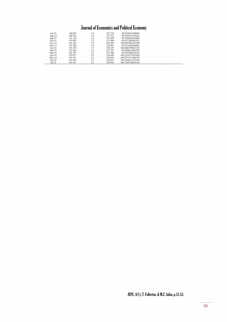
Jul-15 140.853 3.4 237.734 99.8474013428682 Aug-15 140.742 3.4 237.703 99.8343814574432 Sep-15 141.129 3.4 237.489 99.7445022483802 Oct-15 141.007 3.5 237.949 99.9377005482352 Nov-15 141.164 3.5 238.302 100.0859592435590 Dec-15 141.386 3.4 238.041 99.9763402082062 Jan-16 141.270 3.3 238.107 100.0040599642720 Feb-16 141.436 3.3 237.707 99.8360614426593 Mar-16 141.307 3.3 237.920 99.9255206554182 Apr-16 142.017 3.6 238.890 100.3329170703300 May-16 141.791 3.3 239.410 100.5513151484270 Jun-16 141.833 3.7 239.927 100.7684532376120 Jul-16 141.417 4.2 239.828 100.7268736035120



47

47

Table A2. Quarterly Data Date CPI-U: All Items

(Quarterly) CPI

(Q4:2015 = 100) Nominal Retail

Sales Real Retail Sales

Base Period (Q4:2015)

Nominal Total Wages

Real Total Wages Base Period (Q4:2015)

Q1-90 128.033 53.7735267929642 $722,623,502.38 $1,343,827,614.59 $457,397,967.12 $850,600,647.57 Q2-90 129.300 54.3055221114054 $775,774,395.47 $1,428,536,850.97 $461,898,005.10 $850,554,395.10 Q3-90 131.533 55.2435138570781 $727,100,161.58 $1,316,172,905.76 $468,590,810.86 $848,227,743.22 Q4-90 133.767 56.1815056027507 $833,590,747.72 $1,483,745,831.97 $468,329,615.35 $833,601,040.64 Q1-91 134.767 56.6015019067832 $850,499,175.44 $1,502,608,847.44 $477,851,548.05 $844,238,283.35 Q2-91 135.567 56.9374989500092 $807,325,699.24 $1,417,915,634.03 $481,859,213.20 $846,295,011.34 Q3-91 136.600 57.3714951308429 $824,222,981.49 $1,436,641,976.32 $486,354,133.00 $847,727,833.98 Q4-91 137.733 57.8474909420797 $776,673,135.54 $1,342,621,992.58 $478,474,982.71 $827,131,782.07 Q1-92 138.667 58.2394874925101 $823,925,092.79 $1,414,718,996.10 $498,312,769.42 $855,626,982.44 Q2-92 139.733 58.6874835501448 $823,377,935.83 $1,402,987,291.36 $496,200,132.78 $845,495,670.91 Q3-92 140.800 59.1354796077795 $830,995,685.69 $1,405,240,460.04 $501,146,414.09 $847,454,721.62 Q4-92 142.033 59.6534750494196 $792,327,937.89 $1,328,217,571.96 $519,029,153.77 $870,073,626.63 Q1-93 143.067 60.0874712302532 $856,606,231.45 $1,425,598,737.83 $505,763,238.11 $841,711,637.64 Q2-93 144.100 60.5214674110868 $922,785,589.34 $1,524,724,414.01 $526,886,954.68 $870,578,618.16 Q3-93 144.767 60.8014649471085 $978,050,120.64 $1,608,596,308.47 $534,046,956.54 $878,345,541.52 Q4-93 145.967 61.3054605119475 $1,067,259,310.44 $1,740,887,845.11 $553,949,094.44 $903,588,505.52 Q1-94 146.700 61.6134578015714 $983,059,467.03 $1,595,527,182.06 $538,838,003.62 $874,545,956.10 Q2-94 147.533 61.9634547215985 $1,007,761,483.43 $1,626,380,401.09 $549,102,638.88 $886,171,762.61 Q3-94 148.900 62.5374496704429 $1,028,769,617.60 $1,645,045,685.46 $572,412,705.28 $915,311,878.39 Q4-94 149.767 62.9014464672711 $1,174,097,466.65 $1,866,566,720.79 $572,640,707.87 $910,377,646.35 Q1-95 150.867 63.3634424017069 $995,305,215.80 $1,570,787,788.78 $581,444,523.02 $917,634,050.45 Q2-95 152.100 63.8814378433470 $1,067,769,055.80 $1,671,485,633.15 $587,055,300.19 $918,976,341.19 Q3-95 152.867 64.2034350097719 $1,058,838,482.24 $1,649,192,885.21 $587,247,527.60 $914,666,835.99 Q4-95 153.700 64.5534319297990 $1,050,653,590.02 $1,627,572,010.68 $598,844,500.93 $927,672,600.86 Q1-96 155.067 65.1274268786435 $1,025,426,818.45 $1,574,493,063.21 $620,574,360.70 $952,861,782.57 Q2-96 156.400 65.6874219506868 $1,036,844,062.67 $1,578,451,447.60 $615,230,350.39 $936,602,978.34 Q3-96 157.300 66.0654186243161 $1,045,270,303.91 $1,582,174,647.00 $621,764,332.10 $941,134,325.72 Q4-96 158.667 66.6394135731606 $1,037,222,360.30 $1,556,469,819.71 $633,736,934.93 $950,994,165.39 Q1-97 159.633 67.0454100003920 $1,241,455,550.94 $1,851,663,746.90 $640,908,341.94 $955,931,721.40 Q2-97 160.000 67.1994086452039 $1,124,351,412.90 $1,673,156,707.13 $652,170,721.80 $970,500,685.86 Q3-97 160.800 67.5354056884300 $1,187,297,429.44 $1,758,037,013.83 $663,905,301.38 $983,047,772.67 Q4-97 161.667 67.8994024852581 $1,178,888,223.00 $1,736,227,683.67 $683,763,481.14 $1,007,024,297.87 Q1-98 162.000 68.0394012532690 $1,183,048,116.25 $1,738,769,146.20 $680,683,150.81 $1,000,424,957.12 Q2-98 162.533 68.2633992820863 $1,124,473,143.16 $1,647,256,296.91 $713,354,715.86 $1,045,003,213.08 Q3-98 163.367 68.6133962021134 $1,095,725,870.49 $1,596,956,179.31 $703,709,116.37 $1,025,614,756.47 Q4-98 164.133 68.9353933685384 $1,162,585,650.59 $1,686,485,843.89 $720,499,256.02 $1,045,180,452.03 Q1-99 164.733 69.1873911509579 $1,133,007,074.00 $1,637,591,843.18 $684,400,453.48 $989,198,236.98 Q2-99 165.967 69.7053865925980 $1,127,191,441.87 $1,617,079,392.24 $710,274,516.23 $1,018,966,468.66 Q3-99 167.200 70.2233820342381 $1,148,343,605.12 $1,635,272,429.00 $721,604,519.55 $1,027,584,400.88 Q4-99 168.433 70.7413774758782 $1,115,415,678.03 $1,576,751,425.87 $746,239,045.80 $1,054,883,396.99 Q1-00 170.100 71.4413713159324 $1,232,797,520.37 $1,725,607,302.41 $773,016,449.54 $1,082,029,131.44 Q2-00 171.433 72.0013663879758 $1,230,504,582.49 $1,709,001,709.58 $773,146,680.57 $1,073,794,456.07 Q3-00 173.000 72.6593605976268 $1,104,443,035.75 $1,520,028,564.34 $777,360,495.83 $1,069,869,717.32 Q4-00 174.233 73.1773560392669 $1,172,457,899.71 $1,602,214,077.10 $782,951,647.33 $1,069,937,053.90 Q1-01 175.900 73.8773498793211 $1,039,161,379.39 $1,406,603,486.84 $800,172,318.58 $1,083,109,125.99 Q2-01 177.133 74.3953453209612 $1,099,468,551.51 $1,477,872,771.16 $797,190,164.18 $1,071,559,196.00 Q3-01 177.633 74.6053434729775 $1,084,857,141.54 $1,454,127,936.47 $809,655,138.12 $1,085,250,868.68 Q4-01 177.500 74.5493439657731 $1,130,524,173.73 $1,516,477,695.97 $804,326,954.77 $1,078,918,890.47 Q1-02 178.067 74.7873418713916 $ 851,791,801.84 $1,138,951,834.00 $813,282,151.33 $1,087,459,630.18 Q2-02 179.467 75.3753366970371 $872,534,736.90 $1,157,586,519.86 $824,986,078.52 $1,094,504,004.46 Q3-02 180.433 75.7813331242685 $887,221,562.36 $1,170,765,313.55 $839,213,656.92 $1,107,414,744.93 Q4-02 181.500 76.2293291819032 $828,624,707.05 $1,087,015,609.27 $830,567,980.29 $1,089,564,855.42 Q1-03 183.367 77.0133222827639 $876,258,000.89 $1,137,800,545.30 $842,121,244.75 $1,093,474,764.87 Q2-03 183.067 76.8873233915542 $872,725,524.23 $1,135,070,757.75 $838,564,971.97 $1,090,641,389.21 Q3-03 184.433 77.4613183403986 $872,070,306.22 $1,125,813,922.23 $843,807,838.35 $1,089,328,010.98 Q4-03 185.133 77.7553157532214 $882,763,911.81 $1,135,310,046.98 $838,658,096.43 $1,078,586,188.36 Q1-04 186.700 78.4133099628723 $934,700,574.70 $1,192,017,752.02 $857,671,307.14 $1,093,782,812.57 Q2-04 188.167 79.0293045421200 $942,696,204.96 $1,192,843,857.63 $858,683,964.77 $1,086,538,683.01 Q3-04 189.367 79.5333001069591 $948,991,992.64 $1,193,200,824.51 $877,192,784.12 $1,102,925,168.38 Q4-04 191.400 80.3872925918252 $942,882,015.80 $1,172,924,209.04 $898,774,417.35 $1,118,055,339.81 Q1-05 192.367 80.7932890190566 $945,361,363.61 $1,170,098,872.19 $889,668,048.12 $1,101,165,776.17 Q2-05 193.667 81.3392842142989 $956,626,569.68 $1,176,094,157.85 $911,409,816.97 $1,120,503,857.12 Q3-05 196.600 82.5712733727943 $988,814,122.15 $1,197,528,004.31 $946,547,755.97 $1,146,340,267.39 Q4-05 198.433 83.3412665968539 $1,012,685,587.93 $1,215,107,028.35 $935,932,377.26 $1,123,011,942.92 Q1-06 199.467 83.7752627776876 $1,015,335,193.28 $1,211,974,942.97 $996,627,413.36 $1,189,644,031.32 Q2-06 201.267 84.5312561249461 $1,044,340,855.56 $1,235,449,351.44 $989,333,111.90 $1,170,375,500.44 Q3-06 203.167 85.3292491026079 $1,014,369,581.11 $1,188,771,249.93 $974,502,638.85 $1,142,049,940.78 Q4-06 202.333 84.9792521825808 $1,048,528,442.51 $1,233,864,049.85 $987,119,103.08 $1,161,600,129.12 Q1-07 204.317 85.8123848510133 $1,076,253,845.53 $1,254,194,073.96 $992,303,578.47 $1,156,364,061.20 Q2-07 206.631 86.7842562985446 $1,085,298,968.10 $1,250,571,260.72 $1,010,326,848.15 $1,164,182,181.47 Q3-07 207.939 87.3336114642191 $1,079,314,939.33 $1,235,852,864.93 $1,017,545,576.10 $1,165,124,811.68 Q4-07 210.490 88.4048820370381 $1,078,306,431.93 $1,219,736,294.06 $1,036,109,741.34 $1,172,005,117.21 Q1-08 212.770 89.3624736102322 $1,145,600,949.85 $1,281,970,947.72 $1,064,476,569.32 $1,191,189,686.58 Q2-08 215.538 90.5250233797943 $1,140,085,961.49 $1,259,415,263.23 $1,068,130,869.95 $1,179,928,852.89 Q3-08 218.861 91.9208110968624 $1,110,133,938.60 $1,207,706,856.97 $1,084,222,511.62 $1,179,517,998.90 Q4-08 213.849 89.8156496222833 $1,055,423,926.79 $1,175,100,253.94 $1,081,795,656.17 $1,204,462,318.89 Q1-09 212.378 89.1978350590515 $1,006,086,110.58 $1,127,926,602.61 $1,080,532,735.67 $1,211,388,970.32 Q2-09 213.507 89.6721508850722 $1,012,854,592.51 $1,129,508,529.14 $1,071,214,747.93 $1,194,590,223.79 Q3-09 215.344 90.4436840955800 $1,058,193,032.26 $1,170,002,132.09 $1,069,149,814.51 $1,182,116,612.34 Q4-09 217.030 91.1517978641788 $1,065,491,146.96 $1,168,919,507.82 $1,092,659,853.90 $1,198,725,510.09 Q1-10 217.374 91.2962765927660 $1,071,823,010.02 $1,174,005,173.07 $1,069,258,185.30 $1,171,195,830.98 Q2-10 217.297 91.2640768761235 $1,101,007,517.84 $1,206,397,473.71 $1,113,261,995.50 $1,219,824,966.85 Q3-10 217.934 91.5316145217922 $1,060,495,174.14 $1,158,610,803.14 $1,096,155,503.84 $1,197,570,379.99 Q4-10 219.699 92.2727679996416 $1,124,777,986.86 $1,218,970,679.26 $1,150,835,849.04 $1,247,210,714.48 Q1-11 222.044 93.2575193338299 $1,141,461,244.56 $1,223,988,427.65 $1,116,630,301.81 $1,197,362,217.86 Q2-11 224.568 94.3178700027440 $1,188,152,936.45 $1,259,732,579.22 $1,156,929,008.02 $1,226,627,581.80 Q3-11 226.033 94.9328845906156 $1,173,397,183.63 $1,236,028,156.83 $1,169,495,587.31 $1,231,918,309.82 Q4-11 227.047 95.3590408404406 $1,188,492,250.55 $1,246,334,107.47 $1,115,410,358.46 $1,169,695,446.42 Q1-12 228.377 95.9174959260359 $1,260,182,044.67 $1,313,818,748.60 $1,184,492,169.56 $1,234,907,310.83 Q2-12 228.838 96.1111142221949 $1,290,202,989.24 $1,342,407,691.02 $1,175,467,521.69 $1,223,029,751.76 Q3-12 229.769 96.5019907824811 $1,288,976,720.61 $1,335,699,616.30 $1,202,813,130.65 $1,246,412,764.03 Q4-12 231.402 97.1878447469662 $1,288,265,347.32 $1,325,541,636.07 $1,226,365,765.91 $1,261,850,974.37 Q1-13 232.320 97.5734013540681 $1,304,032,383.51 $1,336,462,975.99 $1,232,971,620.41 $1,263,634,969.47 Q2-13 232.036 97.4542624024909 $1,312,957,913.58 $1,347,255,503.46 $1,238,736,728.40 $1,271,095,484.03 Q3-13 233.213 97.9487380511052 $1,290,610,203.57 $1,317,638,419.09 $1,264,233,462.85 $1,290,709,291.41 Q4-13 234.285 98.3989740890280 $1,567,792,589.60 $1,593,301,763.68 $1,260,179,702.74 $1,280,683,781.92 Q1-14 235.651 98.9726890403365 $1,322,070,917.82 $1,335,793,672.62 $1,314,551,784.75 $1,328,196,492.88 Q2-14 236.771 99.4430849008529 $1,393,287,968.81 $1,401,090,855.34 $1,306,902,986.19 $1,314,222,087.43 Q3-14 237.311 99.6696029074944 $1,471,917,164.95 $1,476,796,457.51 $1,336,377,997.41 $1,340,807,988.02 Q4-14 237.125 99.5917635924804 $1,450,191,541.74 $1,456,136,019.11 $1,334,488,571.84 $1,339,958,771.39



48

48

Q1-15 235.409 98.8710499347606 $1,408,840,694.31 $1,424,927,413.28 $1,358,764,002.24 $1,374,278,925.06 Q2-15 236.832 99.4685646766308 $1,393,229,405.99 $1,400,673,077.49 $1,374,718,537.92 $1,382,063,310.54 Q3-15 237.642 99.8087616828972 $1,330,952,080.08 $1,333,502,247.34 $1,391,287,052.37 $1,393,952,824.29 Q4-15 238.097 100 $1,312,994,764.54 $1,312,994,764.54 $1,427,270,033.09 $1,427,270,033.09



49

49

Table A3. Lubbock Business Cycle Index Date Business Cycle Index

Oct-90 99.54696 Nov-90 99.68792 Dec-90 99.71282 Jan-91 99.5577 Feb-91 99.24292 Mar-91 98.69675 Apr-91 98.34103 May-91 98.24249 Jun-91 98.05303 Jul-91 97.95148

Aug-91 97.72679 Sep-91 97.33164 Oct-91 97.29449 Nov-91 97.35037 Dec-91 97.58494 Jan-92 98.16464 Feb-92 98.35432 Mar-92 98.46617 Apr-92 98.7226 May-92 98.81159 Jun-92 99.33646 Jul-92 100

Aug-92 100.3515 Sep-92 100.8378 Oct-92 101.0104 Nov-92 101.0827 Dec-92 101.5741 Jan-93 102.0103 Feb-93 102.7883 Mar-93 103.7544 Apr-93 104.2369 May-93 104.7533 Jun-93 105.16 Jul-93 105.3072






Aug-98 125.1086 Sep-98 125.5011 Oct-98 125.9546 Nov-98 126.1392 Dec-98 126.6932 Jan-99 126.8368 Feb-99 126.7486 Mar-99 127.1143



50

50

Apr-99 127.2139 May-99 127.4379 Jun-99 128.1437 Jul-99 128.6972









Aug-07 137.2929 Sep-07 136.8002 Oct-07 136.9965 Nov-07 137.2391 Dec-07 137.3217



51

51

Jan-08 138.3642 Feb-08 138.7835 Mar-08 138.8032 Apr-08 139.31 May-08 139.0402 Jun-08 138.9988 Jul-08 139.3054











52

52

References Berger, F.D., & Phillips, K.R. (1993). Reassessing Texas employment growth. Federal Reserve Bank of

Dallas Southwest Economy, July/August, 1-3. [Retrieved from]. Berger, F.D., & Phillips, K.R. (1994). Solving the mystery of the disappearing January blip in state

employment data. Federal Reserve Bank of Dallas Economic Review, Second Quarter, 53-62. [Retrieved from].

Burns, A., & Mitchell, W. (1946). Measuring Business Cycles. NBER, New York, NY. Cañas, J., Coronado, R., & Lopez, J.J. (2005). Cyclical differences emerge in border city economies.

Federal Reserve Bank of DallasVista, 2, 1-5. [Retrieved from]. Canas, J., Gilmer, R.W., & Phillips, K. (2003a). A New Index of Coincident Economic Activity for

Houston. Federal Reserve Bank of Dallas Houston Business, April, 1-3. [Retrieved from]. Cañas, J., Gilmer, R.W., & Phillips, K. (2003b). Composite Index: A New Measure of El Paso's Economy.

Federal Reserve Bank of Dallas Business Frontier, 1, 1-4. [Retrieved from]. CB, (2012). Global Business Cycle Indicators. New York, NY: The Conference Board. Clayton-Matthews, A. (2005). DSFM Manual. Boston, MA: University of Massachusetts. Clayton-Matthews, A., & Stock, J.H. (1998/1999).An application of the Stock/Watson index methodology

to the Massachusetts economy, Journal of Economic and Social Measurement, 25(3-4), 183-234. CLPD & LEC. (2000). Lubbock Economic Indicators 1990 - 1999. Lubbock, TX: The City of Lubbock

Planning Department and the Lubbock Economics Council. Diebold, F.X., & Rudebusch, G.D. (1996). Measuring business cycles: A modern perspective, Review of

Economics and Statistics, 78(1), 67-77. doi. 10.2307/2109848 LEDA. (2009). Lubbock, Texas: 2009 Community Profile. Lubbock, TX: Lubbock Economic Development

Alliance. Murphy, A.P. (2005). An Economic Activity Index for Ireland: The Dynamic Single-Factor Method (No

4/RT/05). Dublin, IE: Central Bank and Financial Services Authority of Ireland. [Retrieved from]. Neftici, S.N. (1982). Optimal prediction of cyclical downturns, Journal of Economic Dynamics and Control,

4, 225-241. doi. 10.1016/0165-1889(82)90014-8 Phillips, K.R. (1988). New tools for analyzing the Texas economy: Indexes of coincident and leading

economic indicators. Federal Reserve Bank of Dallas Economic and Financial Policy Review, July, 1-13.

Phillips, K.R. (1998/1999). The composite index of leading economic indicators: A comparison of approaches. Journal of Economic and Social Measurement, 25(3-4), 141-162.

Phillips, K.R. (2005). A New Monthly Index of the Texas Business Cycle. Journal of Economic and Social Measurement, 30(4), 317-333.

Phillips, K.R., & Cañas, J. (2008). Regional business cycle integration along the US–Mexico border. Annals of Regional Science, 42(1), 153-168. doi. 10.1007/s00168-007-0124-8

Phillips, K.R., & Hamden, K.T. (2004). Steady-as-she-goes? An analysis of the San Antonio business cycle. Federal Reserve Bank of Dallas Vista.Winter, 1-6. [Retrieved from].

Stock, J.H., & Watson, M.W. (1989). New indexes of coincident and leading economic indicators.NBER Macroeconomics Annual, 4, 351-409. [Retrieved from].

Stock, J.H., & Watson, M.W. (1991). A probability model of the coincident economic indicators. Chapter 4 in Leading Economic Indicators: New Approaches and Forecasting Records, K. Lahiri & G. Moore (Eds.), Cambridge, UK: Cambridge University Press.

Stock, J.H., & Watson, M.W. (1993). A procedure for predicting recessions with leading indicators: Econometric issues and recent experience. Chapter 2 in Business Cycles, Indicators and Forecasting, J.H. Stock & M.W. Watson (Eds.), Chicago, IL: University of Chicago Press.

Stock, J.H., & Watson, M.W. (1998). Business Cycle Fluctuations in US Macroeconomic Time Series (No. w6528). Cambridge, MA: National Bureau of Economic Research, Inc. doi. 10.3386/w6528

Stock, J.H., & Watson, M.W. (1999). Business cycle fluctuations in US macroeconomic time series, Chapter 1 in Handbook of Macroeconomics, Volume 1A, J.B. Taylor and M. Woodford (eds.), New York, NY: North-Holland.

Tebaldi, E., & Kelly, L. (2012). Measuring Economic Conditions: An Extension of the Stock/Watson Methodology. Applied Economics Letters, 19(18), 1865-1869. doi. 10.1080/13504851.2012.669453

USCB. (2002). United States Census Bureau North American Industry Classification System Concordances, 2002 NAICS to 1987 SIC. Washington, DC: U.S. Department of Commerce.

Copyrights

Copyright for this article is retained by the author(s), with first publication rights granted to

the journal. This is an open-access article distributed under the terms and conditions of the

Creative Commons Attribution license (http://creativecommons.org/licenses/by-nc/4.0).

http://econpapers.repec.org/scripts/redir.pf?u=http%3A%2F%2Fdallasfed.org%2Fassets%2Fdocuments%2Fresearch%2Fswe%2F1993%2Fswe9304a.pdf;h=repec:fip:feddse:y:1993:i:jul:p:1-3:n:4

https://www.google.com.tr/url?sa=t&rct=j&q=&esrc=s&source=web&cd=1&cad=rja&uact=8&ved=0ahUKEwjo-cnBtK7SAhWhKJoKHRcjAykQFggZMAA&url=https%3A%2F%2Fwww.dallasfed.org%2Fassets%2Fdocuments%2Fresearch%2Fer%2F1994%2Fer9402d.pdf&usg=AFQjCNGtvM1oQp-XH5dogEJKQU79P8p

http://dallasfed.org/assets/documents/research/vista/vista0502a.pdf

http://www.dallasfed.org/assets/documents/research/houston/2003/hb0303.pdf

http://www.dallasfed.org/assets/documents/research/busfront/bus0301.pdf

http://dx.doi.org/10.2307/2109848

http://www.centralbank.ie/publications/documents/4RT05.pdf

http://dx.doi.org/10.1016/0165-1889%2882%2990014-8

http://dx.doi.org/10.1007/s00168-007-0124-8

http://dallasfed.org/assets/documents/research/vista/vista0402.pdf

http://papers.nber.org/books/blan89-1

http://dx.doi.org/10.3386/w6528

http://dx.doi.org/10.1080/13504851.2012.669453

Documents

Metropolitan Business Cycle Analysis for Lubbock