Embed Size (px)
Citation preview
June 2019
Metropolitan Adelaide Strategic
Transport Evaluation Model (MASTEM)
MASTEM Version 3 User Guidelines
Cube Base/Voyager


Disclaimer
The application of this guideline does not guarantee that the outputs will be ‘fit-for-purpose’. This guideline only provides a framework for scenario development, testing and subsequent model auditing. Some models, particularly models to be used for financial analysis will require more stringent standards and it is the responsibility of the modeller to ensure that the models they develop are fit for their intended purpose.
This document should only be considered relevant in SA and for no other purpose than as a guide for modellers and managers undertaking work for South Australian Department of Planning, Transport and Infrastructure (DPTI).
DPTI and the authors of this guideline accept no liability or responsibility for any errors or omissions or for any damage or loss arising from the application of the information provided.
Table of Contents
Introduction 8
1.0 Travel Demand Models 10
1.1 General principles 10
1.2 Scenario Testing / Forecasting 11
2.0 MASTEM V3 12
2.1 MASTEM Process 12
2.2 Differences between MASTEM V2 and MASTEM V3 13
2.2.1 General Model Changes 13
2.2.2 Model Application Changes 13
2.2.3 Model Results 14
2.3 Model Structure 15
2.3.1 Overview 15
2.3.2 Prepare Data Files 16
2.3.3 Build Scenario Networks 16
2.3.4 External Vehicle Model 18
2.3.5 Commercial Vehicle Model 19
2.3.6 The Person Trip Generation Model 21
2.3.7 Trip Distribution Model 24
2.3.8 Mode Choice Model 25
2.3.9 Highway and Public Transport (PT) Trip Assignment 27
2.3.10 Final Loop 33
4.0 Model Inputs 42
4.1 Catalog Keys 42
4.1.1 General Model Parameters 42
4.1.2 Highway Inputs 44
4.1.3 Public Transport Inputs 46
5.0 Developing/Running Scenarios 49
5.1 Overview 49
5.2 Socio-Demographics 49
5.3 Highway Network 50
5.3.1 Links and Nodes 50
5.3.2 Junctions and Turn Penalties 50
5.3.3 Parking Costs 51
5.4 Public Transport System 52
5.4.1 PT Lines 52
5.4.2 Walk Access 53
5.4.3 PT Factors File 54
5.4.4 PT System File 54
5.4.5 PT Fares Files 55
5.4.6 PT Park, Kiss and Ride Stations Files 55
5.4.7 PT Interchanges File 57
5.5 Public Transport priority 57
5.5.1 Bus Lanes 57
5.5.2 Junction Priority 57
6.0 Model Outputs 58
6.1 Scenario Reporting 58
6.2 Loaded Highway and Pubic Transport Networks 60
6.3 Report Tool Overview and Its Contents 63
6.4 MASTEM User Benefit Calculation Tool (MUBCT) 66
6.4.1 MASTEM Outputs 66
6.4.2 MUBCT 66
6.5 Using Model Outputs 67
7.0 Model Auditing 67
7.1 MASTEM Audit Checklist 67
Appendix A – MASTEM Model Structure 68
Appendix B – Foundation Network Updating 95
Appendix C – Public Transport Input Files Updating 122
Appendix D – Highway Input Files Updating 129
Appendix E - MASTEM User Benefit Calculation Tool 132
Appendix F – MASTEM Audit Check List 140
List of Tables
Table 2-1 Description of Build Scenario Network Programs ................................................. 17
Table 2-2 Description of External Vehicle Model Programs ................................................. 18
Table 2-3 Description of Commercial Vehicle Model Programs ........................................... 19
Table 2-4 Description of Person Trip Generation Model Programs ...................................... 23
Table 2-5 Description of Trip Distribution Model Programs .................................................. 24
Table 2-6 Description of Mode Choice Model Programs ...................................................... 26
Table 2-7 Description of Highway and PT Trip Assignment Model Programs ...................... 28
Table 2-8 Description of the AM Time Period Model Programs ............................................ 29
Table 2-9 Description of the DT Time Period Model Programs ............................................ 30
Table 2-10 Description of the PM Time Period Model Programs .......................................... 31
Table 2-11 Description of the NT Time Period Model Programs .......................................... 32
Table 2-12 Description of the Next Loop Model Programs ................................................... 33
Table 2-13 Description of the Final Loop Model Programs ................................................... 35
Table 2-14 Describes the Final PT Trip Assignment Model Programs ................................. 36
Table 2-15 Describes the Model Calibration Statistics Programs ......................................... 37
Table 2-16 Describes the PT Assignment Statistics Programs ............................................ 37
Table 2-17 Describes the PT Trip Distributions Programs .................................................... 38
Table 2-18 Describes the Highway Assignment Statistics Programs ................................... 38
Table 2-19 Describes the Highway Screenlines and Travel Times Statistics Programs ....... 40
Table 2-20 Describes the Highway Trip Distributions Programs .......................................... 40
Table 2-21 Describes the MUBCT and Accessibility Calculations Programs ....................... 41
Table 2-22 Describes the Scenario Reporting Programs ..................................................... 41
Table 4-1 General Model Parameters – Catalog Keys ......................................................... 43
Table 4-2 Highway Inputs - Catalog Keys ............................................................................. 45
Table 4-3 Public Transport Inputs - Catalog Keys ................................................................ 47
Table 5-1 MASTEM Job Type Categories ............................................................................ 49
Table 5-2 MASTEM Education Type Categories .................................................................. 50
Table 5-3 - Public Transport Line file Inputs ......................................................................... 52
Table 6-1 Link Attribute List for Final Loaded Highway Network .......................................... 61
Table 6-2 Link Attributes List for Final Loaded Public Transport Network ............................ 62
Table 6-3 Reporting Tool Contents ....................................................................................... 63

List of Figures
Figure 2.1 Mechanisms of a transport model ........................................................................ 10
Figure 3.1 MASTEM Process ............................................................................................... 12
Figure 3.2 MASTEM main modal structure ........................................................................... 15
Figure 3.3 Build Scenario Networks Applications ................................................................. 16
Figure 3.4 External Vehicle Model ........................................................................................ 18
Figure 3.5 Commercial Vehicle Model Overview .................................................................. 19
Figure 3.6 Person Trip Generation Model Application – part A ............................................ 21
Figure 3.7 Trip Generation Model Application – part B ......................................................... 22
Figure 3.8 Trip Distribution Model Application ...................................................................... 24
Figure 3.9 Mode Choice Model Application .......................................................................... 25
Figure 3.10 Highway and PT Assignment ............................................................................. 27
Figure 3.11 Final Loop - Hwy and PT Trip Assignment Model ............................................. 34
Figure 4.1 Scenario Manager – General Model Parameters ................................................ 42
Figure 4.2 Scenario Manager - Highway Inputs .................................................................... 44
Figure 4.3 Scenario Manager - Public Transport Inputs ....................................................... 46
Figure 4.4 Access modes applicable for three public transport user classes ....................... 48
Figure 5.1 - Walk Link Distance for Built-Up Urban Area ...................................................... 54
Figure 5.2 - Representation of Park and Ride Function ........................................................ 56
Figure 6.1 Scenario Reporting - Calibration Results Workbook - Start Worksheet............... 58
Figure 6.2 - Scenario Reporting - Summary Results Workbook, Start Worksheet ............... 59
Figure 6.3 - Scenario Reporting - Screenlines Results Workbook, Start Worksheet ............ 59
Figure 6.4 - Scenario Reporting – PT Lines Workbook – Start Worksheet ........................... 60
Figure 6.5 - MUBCT - Main input page ................................................................................. 66
Introduction
The Department of Planning, Transport and Infrastructure (DPTI) works as part of the
community to deliver effective planning policy, efficient transport, and valuable social and
economic infrastructure. As part of this task DPTI must ensure that the effects of all planned
interventions on the strategic road network and proposed developments which are likely to
impact this network are thoroughly understood before they are implemented. Comprehensive
and accurate modelling which is fit for the intended purpose is necessary to ensure these
interventions and proposals can be:
fully assessed for impacts and benefits
effectively designed to satisfy the original objectives and mitigate any adverse impacts
clarified to avoid confusion or misinterpretation as the design is developed, and
effectively and efficiently implemented and operated
A common definition of the term ‘model’ in its most general form is:
“A model can be defined as a simplified representation of a part of the real
world………which concentrates on certain elements considered important for its
analysis from a particular point of view.”1
It is important to be aware of the simplifications and assumptions that have been made in
creating any model and to understand how these affect overall model performance. These
simplifications and assumptions can derive from decisions made by the modeller during model
development or calibration, or can be inherent to the particular choice of modelling software
used.
DPTI uses a range of analytical tools to assess road network performance and to plan future
development of the network. The Metropolitan Adelaide Strategic Transport Evaluation Model
(MASTEM) is DPTI’s preferred strategic travel demand model built within the Cube software
package by Citilabs. This guide has been developed to provide broad guidance on the overall
process of using MASTEM within the Cube package.
This guide covers the broad areas of model structure, model inputs, model outputs,
documenting and auditing, and is to be used as the primary guide for development of
modelling scenarios for use within DPTI. It draws upon experience and expertise from across
the Agency and the industry more broadly and forms a comprehensive source of best practice.
It is intended that this guide will be regularly reviewed and updated so that it remains current,
useful and relevant for users. This version of the guide relates to Cube 6.4.x and MASTEM
V3.1.x, which are the current versions used within DPTI. Before undertaking any travel
demand modelling, practitioners should ensure that they have the latest version of this
document – which is available on DPTI’s internet site – and that they discuss their modelling
proposal with appropriate staff within DPTI.
In April 2009, the then Department of Transport, Energy and Infrastructure (DTEI) now the
Department of Planning Transport and Infrastructure (DPTI), appointed the consultant
AECOM to update the Metropolitan Adelaide Strategic Evaluation Model (MASTEM) – then
1 Ortúzar J de D & Willumsen L G, Modelling Transport, 4th Ed., Ch1, Wiley, London, 2011, p2.

MASTEM V2.2.2. This work was to focus on the enhancement of the model’s public transport
modelling capabilities and included an expansion of the model coverage to Mount Barker area
as well as other areas identified for future development by the 30 Year Development Plan for
Greater Adelaide. The model developed as a result of this work is designated as MASTEM
V3.0.
In late 2010, DPTI began a major review of the consultant’s work with a view to further
developing the model for production use within the Agency and by external Consultants. This
process has resulted in significant corrections/changes to the model developed by AECOM.
As part of this work, significant changes were made to the Foundation Network aimed at
improving the accuracy of the Highway assignment processes, as well as significant changes
to the MASTEM Reporting Tool. The model developed as a result of this work is designated
as MASTEM V3.1 and is the subject of this Guideline.
1.0 Travel Demand Models
At the highest level, travel demand models link estimates of travel demand and transportation
system performance to land-use patterns, socio-demographics, employment, transportation
infrastructure, and transportation policies. Most travel demand models – including MASTEM
- represent the classical "four-step" strategic modelling process involving trip generation, trip
distribution, mode choice, and trip assignment. This process broadly answers the following
four questions:
How many people are going to travel?
Where are they going to travel to and from?
What transportation mode are they going to use to get there?
What route will they take to get there?
1.1 General principles
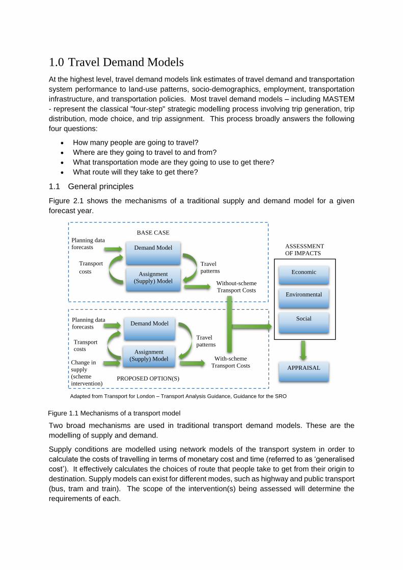
Figure 2.1 shows the mechanisms of a traditional supply and demand model for a given
forecast year.
Two broad mechanisms are used in traditional transport demand models. These are the
modelling of supply and demand.
Supply conditions are modelled using network models of the transport system in order to
calculate the costs of travelling in terms of monetary cost and time (referred to as ‘generalised
cost’). It effectively calculates the choices of route that people take to get from their origin to
destination. Supply models can exist for different modes, such as highway and public transport
(bus, tram and train). The scope of the intervention(s) being assessed will determine the
requirements of each.
Transport
costs
Demand Model
Assignment
(Supply) Model
Travel
patterns
Planning data
forecasts
Without-scheme
Transport Costs
BASE CASE
Demand Model
Assignment
(Supply) Model
Transport
costs
Travel
patterns
Planning data
forecasts
With-scheme
Transport Costs
PROPOSED OPTION(S)
Change in
supply
(scheme
intervention)
Economic
Environmental
Social
ASSESSMENT
OF IMPACTS
APPRAISAL
Adapted from Transport for London – Transport Analysis Guidance, Guidance for the SRO
Figure 1.1 Mechanisms of a transport model

Demand models are required to ascertain the change in travel behaviour of individuals in
reaction to the changes in cost from the changed supply conditions. For example, where car
congestion on the roads increases over time, people may decide to shift to public transport
modes, travel to alternative locations or even travel less. The demand model takes these
responses into consideration and simulates the choices that people make given the options
that are available to them.
The demand model is fed with future year planning data, for example forecasts of future
population, dwellings, employment and education, which drive future travel demand. The
supply model then provides updated travel costs for individuals, based on the forecast level of
demand (e.g. more people on the road will cause higher transport costs for existing users).
The model seeks to balance supply and demand i.e. when small changes in costs do not
cause significant changes in demand and vice versa. This state is referred to as equilibrium.
It is important to achieve equilibrium since failure to do so will produce misleading results that
are not a reliable basis for intervention appraisal.
1.2 Scenario Testing / Forecasting
Models can also be used to run “what if?” scenarios where changes in input assumptions may
be tested. This can help in assessing options before a preferred intervention is brought
forward. It can also be used to present “sensitivity tests” around the final appraisal results to
account for uncertainty that may occur in real life.
Assessment of any intervention (transport or otherwise) requires an appreciation of expected
future benefits and disbenefits. Being in the future, these benefits and disbenefits cannot be
measured or observed at the time the decision needs to be made, and so they need to be
estimated by comparing two forecasts – one excluding the intervention, the other including the
intervention and no other changes.
These two forecasts are generally called the ’base case’ forecast and ’project case’ forecast
respectively (see figure 2.1). Often, separate pairs of forecasts are required for at least two
forecast years, to take into account changes in both demographic and other transport
infrastructure over time.
The appraisal uses the model outputs to assess the impacts of the intervention in terms of
economic costs and benefits, environmental impacts such as noise and air quality, and social
impacts such as severance, accessibility and distributional equity. To assess the transport
and social impacts of any intervention the ‘base case’ is usually based on a supply model
where no changes have been made above ‘business as usual’ conditions. The ‘project case’
then adds the intervention(s) being tested. To assess the economic impacts of any
intervention the ‘base case’ is usually based on a supply model where no changes have been
made above either ‘do nothing’ or ‘do minimum’ conditions. Again, the ‘project case’ then
adds the intervention(s) being tested.
In order for forecasts to be credible, the assumptions need to be realistic. Also, as different
transport intervention often compete for a common budget, it is important that the forecasting
assumptions are consistent and unbiased so that the budget can be allocated on a fair basis.
Good practice requires that modifications to the transport network are tested under different
input assumptions (compiled as alternative scenarios or sensitivity tests) to highlight any risks
to the benefits or impacts of the intervention. Alternative scenarios or sensitivity tests should
cover any significant sources of uncertainty, but their use should be proportionate.
2.0 MASTEM V3
2.1 MASTEM Process
The Metropolitan Adelaide Strategic Transport Evaluation Model (MASTEM) is a
comprehensive multi-modal urban travel demand model suite, which is used to prepare
forecasts of travel demand for selected future years (i.e. 2021, 2026, 2031 and 2036) that are
consistent with the State Government’s demographic and land use policies and plans.
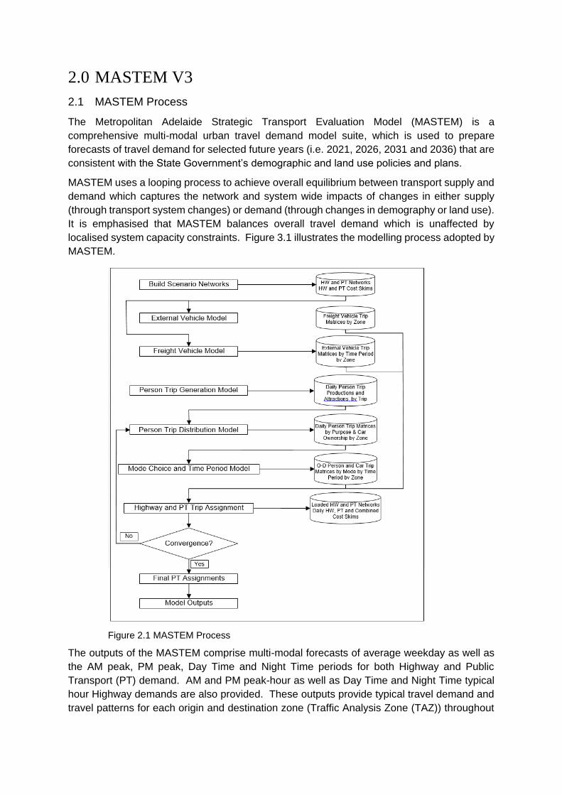
MASTEM uses a looping process to achieve overall equilibrium between transport supply and
demand which captures the network and system wide impacts of changes in either supply
(through transport system changes) or demand (through changes in demography or land use).
It is emphasised that MASTEM balances overall travel demand which is unaffected by
localised system capacity constraints. Figure 3.1 illustrates the modelling process adopted by
MASTEM.
The outputs of the MASTEM comprise multi-modal forecasts of average weekday as well as
the AM peak, PM peak, Day Time and Night Time periods for both Highway and Public
Transport (PT) demand. AM and PM peak-hour as well as Day Time and Night Time typical
hour Highway demands are also provided. These outputs provide typical travel demand and
travel patterns for each origin and destination zone (Traffic Analysis Zone (TAZ)) throughout
Figure 2.1 MASTEM Process
the scope of the model on both the arterial (and major local) road network and the Adelaide
Metro (train, tram and bus) public transport system. Average weekday demands for walking
and cycling are also provided.
2.2 Differences between MASTEM V2 and MASTEM V3
2.2.1 General Model Changes
Key changes in MASTEM V3 in comparison to MASTEM V2 include:
Time periods: Four model time periods have been developed within MASTEM V3:
AM peak period – 7 am to 9 am for both Highway and PT
Day Time period – 9 am to 4 pm for Highway and 9 am to 3 pm for PT
PM peak period – 4 pm to 7 pm for Highway and 3 pm to 6 pm for PT
Night Time period – 7 pm to 7 am for Highway and 6 pm to 7 am for PT
It should be noted that for both of Highway and PT travel, daily results are reported. In
addition, for Highway travel, results are reported for the AM peak hour (nominally 8 am
to 9 am), the PM peak hour (nominally 5 pm to 6 pm) as well as a “typical hour” for
each of the day time and night time periods, whereas for PT travel, results are reported
for the four model time periods.
Model Zones: The number of model zones has been increased from 320 to 634 by
splitting a number of large zones and also by expanding the model coverage to include
Mount Barker, Roseworthy, Gawler East and part of the Barossa Valley.
Model Inputs: All scenario specific model inputs are via Catalog Keys.
2.2.2 Model Application Changes
Build Scenario Networks application: This application was changed so that the primary
input is now a foundation network for the model run, rather than a series of link and
node files. This network can either be a standalone *.net file or part of a Geodatabase
(*.gdb), which may also include many of the other scenario specific network related
inputs such as the Highway Junction files and the PT Lines files. A further key change
to the model inputs is that only one PT Lines file incorporating all necessary data for
all model time periods (those described above plus the complete day) is now required.
This application was also modified to generate many of the files necessary to support
the extraction of model outputs.
External and Freight Vehicle Model applications: Both of these applications were
modified to provide for the expanded zone system and to simplify the processing of
these applications.
Person Trip Generation Model application: This application was created by merging a
number of related applications, many of which contained only one or two programs.
The steps now included in this application are:
Household Stratification by Residents, Workers and Dependants
Car Ownership Model
Household Stratification by Car Ownership
Trip End Generation
Travel Market Segmentation

The approach adopted to the balancing of trip productions and attractions in both the
Trip End Generation and the Travel Market Segmentation processes balances trip
ends separately across the MASTEM V2 model coverage and the added zones within
the Mount Barker area and the Gawler East/Barossa Valley/Roseworthy area.
Trip Distribution Model application: This application was modified so that the
generalised cost are now based on the composite daily cost for Highway and PT
modes so that the trip distribution process can take into account traffic congestion on
the Highway network and also improvements to the PT system.
Mode Choice Model application: This application was modified so that the input skim
cost for both Highway and PT represent generalised cost and generalised time as
appropriate. A sub-mode choice model which splits the daily PT demand into
walk/ride/walk trips and park & ride trips has been added. The application has also
been modified to reflect the change from three time periods across the day to four.
Highway and PT Trip Assignment application: This application now includes both
Highway and PT assignments which are carried out for each of the four time periods.
The Highway assignment process now includes park and ride cars and buses. The
application was also modified to extract congested network attributes from the Highway
assignments for input into the PT assignment process and also to consider the effect
of bus priority at signalised intersections. The PT assignment process was significantly
modified to:
enable the assignment for the three user class demand matrices separately
consider the effect of parking capacity on park and ride demand
apply different mid-block speeds for express buses and stopping buses
include the effect of dedicated bus lanes and of bus priority at signalised
intersections
include the effect of crowding on the operation of the PT system (optional
process that needs to be selected prior to running a scenario)
2.2.3 Model Results
Model Outputs: All scenario specific model outputs are accessible via the MASTEM
Reporting Tool which provides a convenient way to access/analysis any required
model outputs.
A multi-faceted MASTEM Reporting Tool which is based on Microsoft Excel has also
been developed which enables:
the reporting a range of model performance / calibration summary statistics
the reporting of a range of Highway and PT assignment summary statistics
the analysis of a range of Highway and PT assignment results
The components of this tool can be accessed from the Scenario Reporting application,
although it should be noted that it may be necessary to allow / activate Excel macro operation.

For details of the initial development of MASTEM Version 3 refer to “Enhanced Public
Transport Modelling, Model Development and Validation Report”2 prepared by AECOM in
March 2010. For further details of the re-development of this initial version refer to
“Metropolitan Adelaide Strategic Transport Evaluation Model, MASTEM Version 3, Model Re-
development, Calibration / Validation Report”3 updated by DPTI in February 2018.
2.3 Model Structure
The following sections provide an overview in a graphical and tabular form to describe the
applications and programs used within the MASTEM model. The full MASTEM model
graphical flow-chart style user interface can be seen in Appendix A.
2.3.1 Overview
Figure 3.2 shows the overall model structure of MASTEM V3.
The following applications/programs are describe in more details in the next sections.
Build Scenario Networks (Box 2)
External Vehicle Model (Box 4)
Commercial Vehicle Model (Box 7)
2 Department of Transport, Energy and Infrastructure (2009), Enhanced Public Transport Modelling, Model
Development and Validation Report, prepared by AECOM. 3 Department of Planning, Transport and Infrastructure, MASTEM V3.1, Model Re-Development and
Validation Report (2018)
Figure 2.2 MASTEM main modal structure

Person Trip Generation Model (Box 10)
Trip Distribution Model (Box 15)
Mode Choice Model (Box 16)
Highway ad Public Transport Trip Assignment (Box 17)
Within the MASTEM model structure a number of Pilot, Cluster and Loop programs are used.
These programs enable a more dynamic and efficient modelling process. They are:
Pilot: Starts the Cube Cluster nodes and waits until all of the previous Clusters steps
are complete.
Cluster: Starts/Ends the processing of the associated applications/programs in
parallel.
Loop: Controls the model looping process and updates the files for the next loop.
2.3.2 Prepare Data Files
This application, prebuild contains a number of programmes which were developed to assist
the creation of a range of input data files. Some of these may be useful when developing
project specific model inputs. Note: This application and programs are not run as part of the
modelling process. For the model flowchart see Appendix A: Figure A.1.
2.3.3 Build Scenario Networks
Figure 3.3 shows the application program for the Build Scenario Networks.
Table 3.1 describes the functions of each program in the Build Scenario Networks. The first
column is the program and associated box run order number. The second column being the
description, describing what the program does.
Figure 2.3 Build Scenario Networks Applications
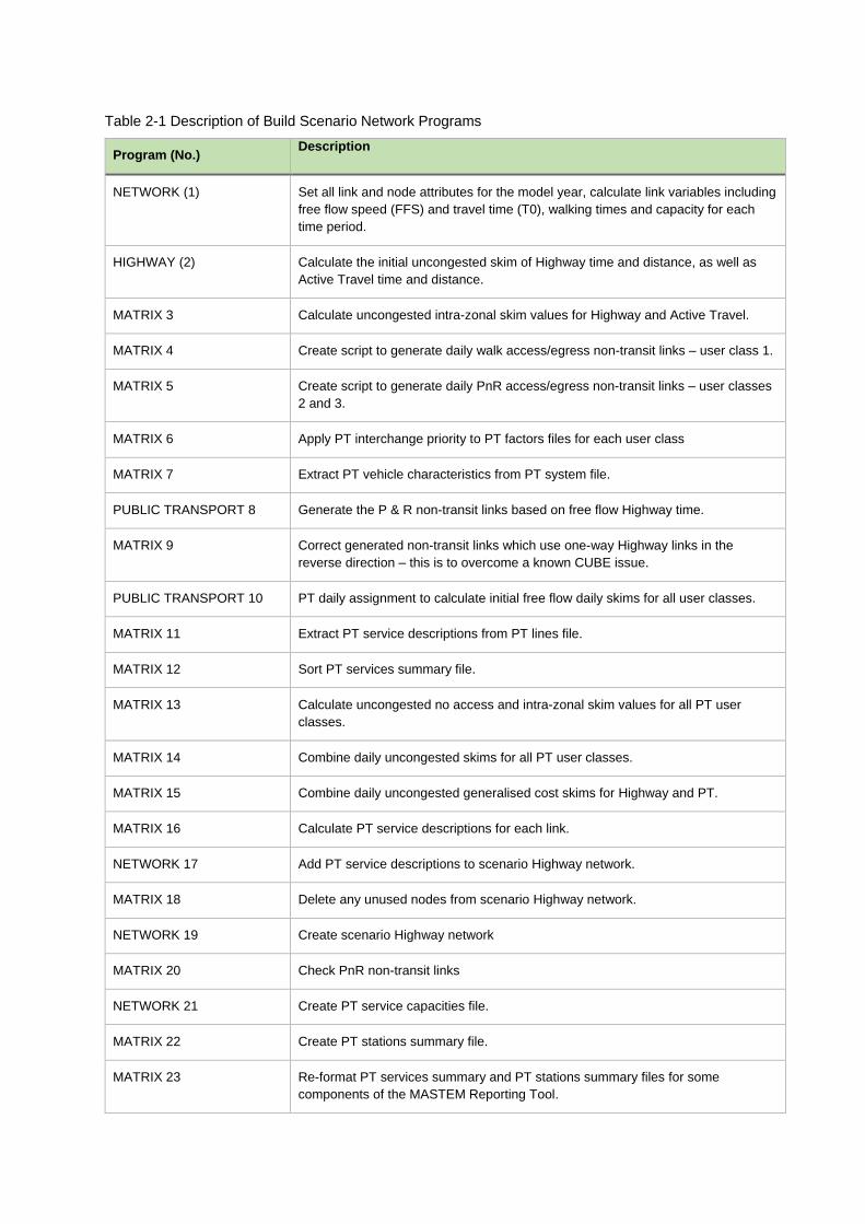
Program (No.) Description
NETWORK (1) Set all link and node attributes for the model year, calculate link variables including
free flow speed (FFS) and travel time (T0), walking times and capacity for each
time period.
HIGHWAY (2) Calculate the initial uncongested skim of Highway time and distance, as well as
Active Travel time and distance.
MATRIX 3 Calculate uncongested intra-zonal skim values for Highway and Active Travel.
MATRIX 4 Create script to generate daily walk access/egress non-transit links – user class 1.
MATRIX 5 Create script to generate daily PnR access/egress non-transit links – user classes
2 and 3.
MATRIX 6 Apply PT interchange priority to PT factors files for each user class
MATRIX 7 Extract PT vehicle characteristics from PT system file.
PUBLIC TRANSPORT 8 Generate the P & R non-transit links based on free flow Highway time.
MATRIX 9 Correct generated non-transit links which use one-way Highway links in the
reverse direction – this is to overcome a known CUBE issue.
PUBLIC TRANSPORT 10 PT daily assignment to calculate initial free flow daily skims for all user classes.
MATRIX 11 Extract PT service descriptions from PT lines file.
MATRIX 12 Sort PT services summary file.
MATRIX 13 Calculate uncongested no access and intra-zonal skim values for all PT user
classes.
MATRIX 14 Combine daily uncongested skims for all PT user classes.
MATRIX 15 Combine daily uncongested generalised cost skims for Highway and PT.
MATRIX 16 Calculate PT service descriptions for each link.
NETWORK 17 Add PT service descriptions to scenario Highway network.
MATRIX 18 Delete any unused nodes from scenario Highway network.
NETWORK 19 Create scenario Highway network
MATRIX 20 Check PnR non-transit links
NETWORK 21 Create PT service capacities file.
MATRIX 22 Create PT stations summary file.
MATRIX 23 Re-format PT services summary and PT stations summary files for some
components of the MASTEM Reporting Tool.
Table 2-1 Description of Build Scenario Network Programs
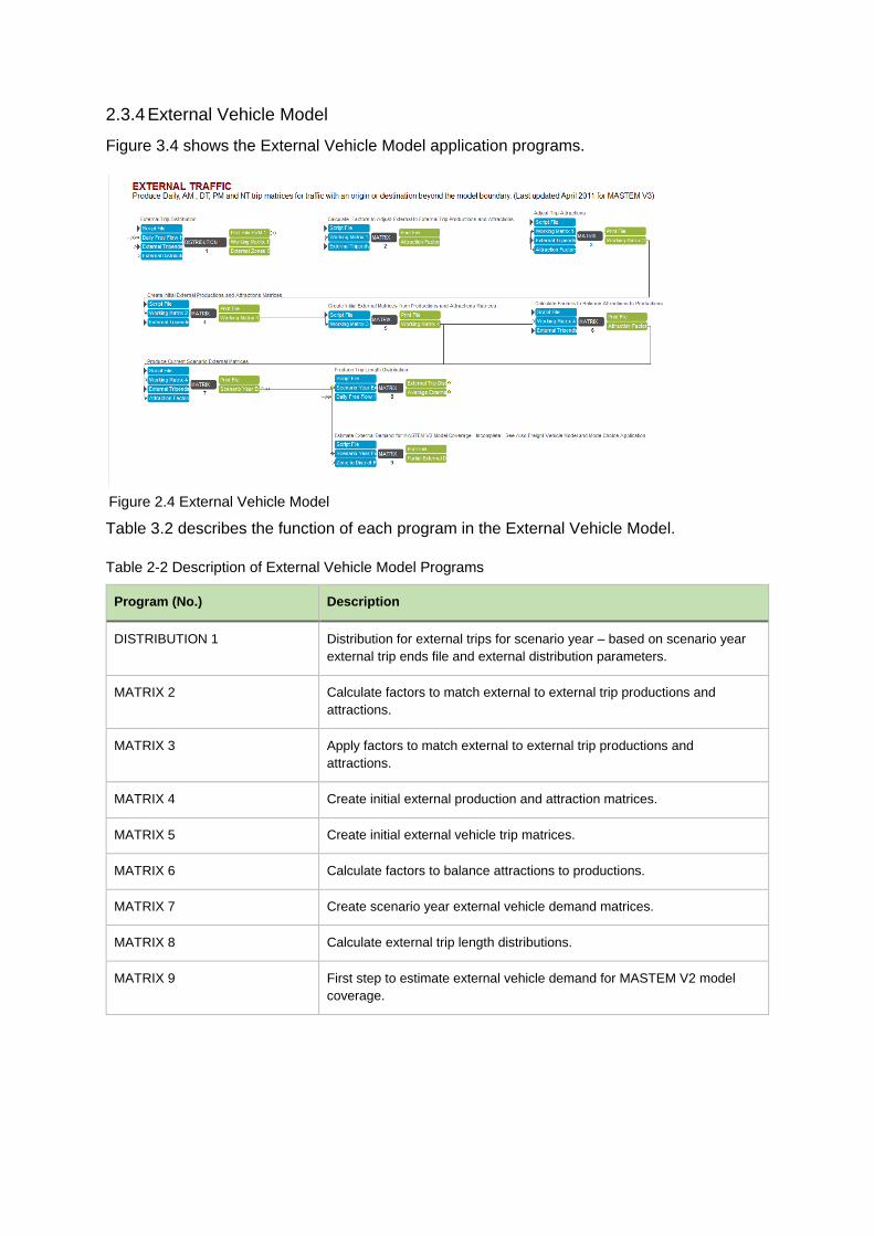
2.3.4 External Vehicle Model
Figure 3.4 shows the External Vehicle Model application programs.
Table 3.2 describes the function of each program in the External Vehicle Model.
Program (No.) Description
DISTRIBUTION 1 Distribution for external trips for scenario year – based on scenario year
external trip ends file and external distribution parameters.
MATRIX 2 Calculate factors to match external to external trip productions and
attractions.
MATRIX 3 Apply factors to match external to external trip productions and
attractions.
MATRIX 4 Create initial external production and attraction matrices.
MATRIX 5 Create initial external vehicle trip matrices.
MATRIX 6 Calculate factors to balance attractions to productions.
MATRIX 7 Create scenario year external vehicle demand matrices.
MATRIX 8 Calculate external trip length distributions.
MATRIX 9 First step to estimate external vehicle demand for MASTEM V2 model
coverage.
Table 2-2 Description of External Vehicle Model Programs
Figure 2.4 External Vehicle Model
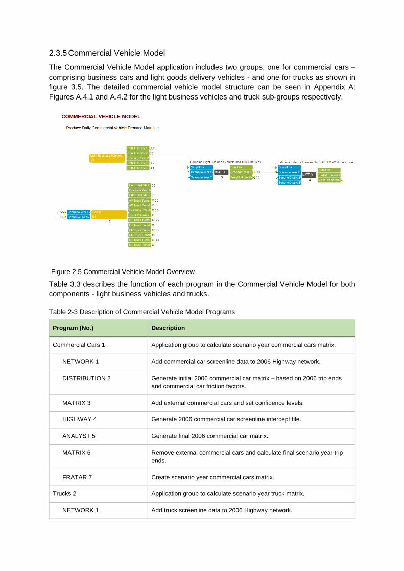
2.3.5 Commercial Vehicle Model
The Commercial Vehicle Model application includes two groups, one for commercial cars –
comprising business cars and light goods delivery vehicles - and one for trucks as shown in
figure 3.5. The detailed commercial vehicle model structure can be seen in Appendix A:
Figures A.4.1 and A.4.2 for the light business vehicles and truck sub-groups respectively.
Table 3.3 describes the function of each program in the Commercial Vehicle Model for both
components - light business vehicles and trucks.
Program (No.) Description
Commercial Cars 1 Application group to calculate scenario year commercial cars matrix.
NETWORK 1 Add commercial car screenline data to 2006 Highway network.
DISTRIBUTION 2 Generate initial 2006 commercial car matrix – based on 2006 trip ends
and commercial car friction factors.
MATRIX 3 Add external commercial cars and set confidence levels.
HIGHWAY 4 Generate 2006 commercial car screenline intercept file.
ANALYST 5 Generate final 2006 commercial car matrix.
MATRIX 6 Remove external commercial cars and calculate final scenario year trip
ends.
FRATAR 7 Create scenario year commercial cars matrix.
Trucks 2 Application group to calculate scenario year truck matrix.
NETWORK 1 Add truck screenline data to 2006 Highway network.
Table 2-3 Description of Commercial Vehicle Model Programs
Figure 2.5 Commercial Vehicle Model Overview

Program (No.) Description
DISTRIBUTION 1 Generate initial 2006 truck matrix – based on 2006 trip ends and truck
friction factors.
MATRIX 3 Add external trucks and set confidence levels.
HIGHWAY 4 Generate 2006 truck screenline intercept file.
ANALYST 5 Generate final 2006 truck matrix.
MATRIX 6 Adjust scenario year truck trip ends to match BITRE growth rates.
MATRIX 7 Remove external trucks and calculate final scenario year trip ends.
FRATAR 8 Create scenario year truck matrix.
MATRIX 3 Combine commercial cars and trucks scenario year matrices
MATRIX 4 Second step to estimate external vehicle demand for MASTEM V2 model
coverage.
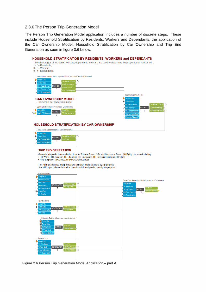
2.3.6 The Person Trip Generation Model
The Person Trip Generation Model application includes a number of discrete steps. These
include Household Stratification by Residents, Workers and Dependants, the application of
the Car Ownership Model, Household Stratification by Car Ownership and Trip End
Generation as seen in figure 3.6 below.
Figure 2.6 Person Trip Generation Model Application – part A
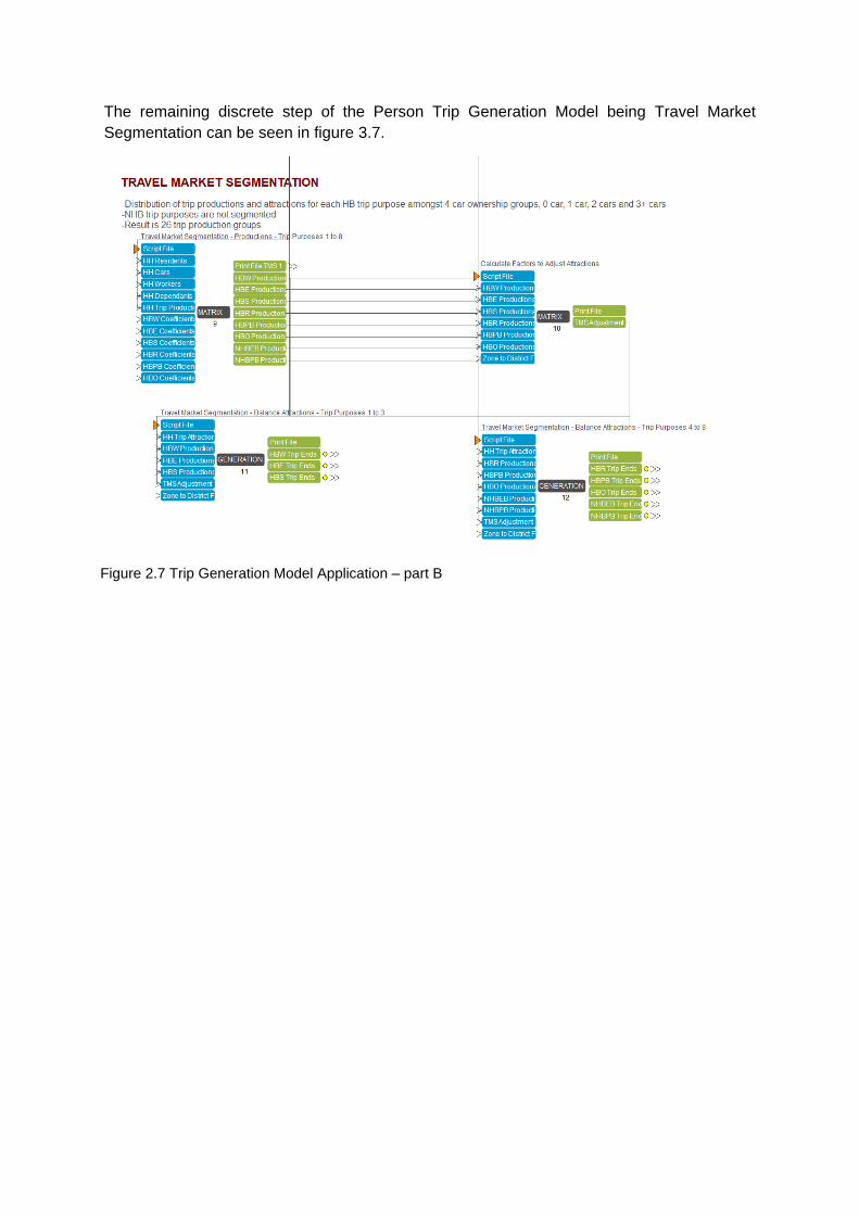
The remaining discrete step of the Person Trip Generation Model being Travel Market
Segmentation can be seen in figure 3.7.
Figure 2.7 Trip Generation Model Application – part B
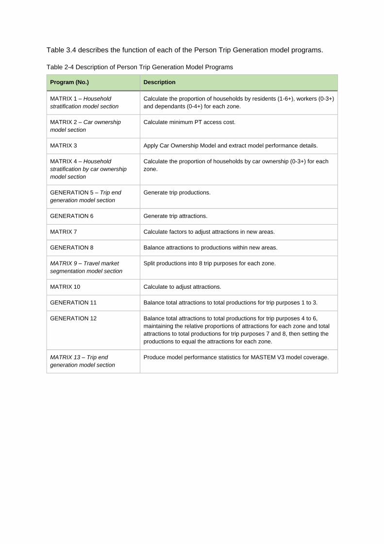
Table 3.4 describes the function of each of the Person Trip Generation model programs.
Program (No.) Description
MATRIX 1 – Household
stratification model section
Calculate the proportion of households by residents (1-6+), workers (0-3+)
and dependants (0-4+) for each zone.
MATRIX 2 – Car ownership
model section
Calculate minimum PT access cost.
MATRIX 3 Apply Car Ownership Model and extract model performance details.
MATRIX 4 – Household
stratification by car ownership
model section
Calculate the proportion of households by car ownership (0-3+) for each
zone.
GENERATION 5 – Trip end
generation model section
Generate trip productions.
GENERATION 6 Generate trip attractions.
MATRIX 7 Calculate factors to adjust attractions in new areas.
GENERATION 8 Balance attractions to productions within new areas.
MATRIX 9 – Travel market
segmentation model section
Split productions into 8 trip purposes for each zone.
MATRIX 10 Calculate to adjust attractions.
GENERATION 11 Balance total attractions to total productions for trip purposes 1 to 3.
GENERATION 12 Balance total attractions to total productions for trip purposes 4 to 6,
maintaining the relative proportions of attractions for each zone and total
attractions to total productions for trip purposes 7 and 8, then setting the
productions to equal the attractions for each zone.
MATRIX 13 – Trip end
generation model section
Produce model performance statistics for MASTEM V3 model coverage.
Table 2-4 Description of Person Trip Generation Model Programs
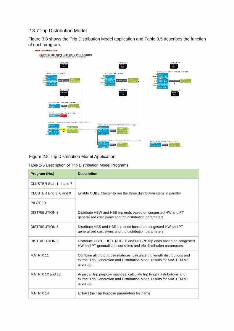
2.3.7 Trip Distribution Model
Figure 3.8 shows the Trip Distribution Model application and Table 3.5 describes the function
of each program.
Program (No.) Description
CLUSTER Start 1, 4 and 7
Enable CUBE Cluster to run the three distribution steps in parallel. CLUSTER End 3, 6 and 9
PILOT 10
DISTRIBUTION 2 Distribute HBW and HBE trip ends based on congested HW and PT
generalised cost skims and trip distribution parameters.
DISTRIBUTION 5 Distribute HBS and HBR trip ends based on congested HW and PT
generalised cost skims and trip distribution parameters.
DISTRIBUTION 5 Distribute HBPB, HBO, NHBEB and NHBPB trip ends based on congested
HW and PT generalised cost skims and trip distribution parameters.
MATRIX 11 Combine all trip purpose matrices, calculate trip length distributions and
extract Trip Generation and Distribution Model results for MASTEM V3
coverage.
MATRIX 12 and 13 Adjust all trip purpose matrices, calculate trip length distributions and
extract Trip Generation and Distribution Model results for MASTEM V2
coverage.
MATRIX 14 Extract the Trip Purpose parameters file name.
Table 2-5 Description of Trip Distribution Model Programs
Figure 2.8 Trip Distribution Model Application

2.3.8 Mode Choice Model
The Mode Choice Model application initially performs the mode split – into car
driver/passenger, public transport, walking and cycling. The outputs of this process is then
further processed in two separate groups, which split the PT and Highway daily demand
matrices into the four time periods (see Appendix A: Figure A.8.1 for the detailed Public
Transport and Highway time period demand subgroup model programs). Figure 3.9 shows
the Mode Choice Model applications and Table 3.6 describes the function of each program.
Figure 2.9 Mode Choice Model Application
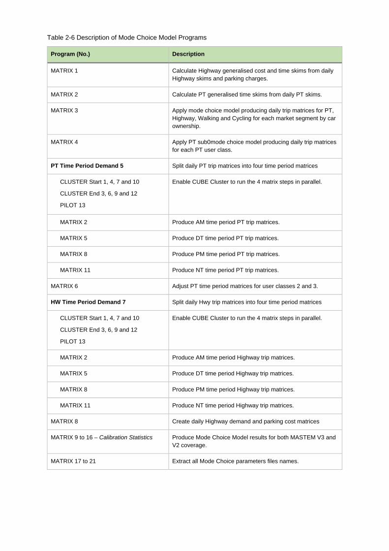
Program (No.) Description
MATRIX 1 Calculate Highway generalised cost and time skims from daily
Highway skims and parking charges.
MATRIX 2 Calculate PT generalised time skims from daily PT skims.
MATRIX 3 Apply mode choice model producing daily trip matrices for PT,
Highway, Walking and Cycling for each market segment by car
ownership.
MATRIX 4 Apply PT sub0mode choice model producing daily trip matrices
for each PT user class.
PT Time Period Demand 5 Split daily PT trip matrices into four time period matrices
CLUSTER Start 1, 4, 7 and 10
CLUSTER End 3, 6, 9 and 12
PILOT 13
Enable CUBE Cluster to run the 4 matrix steps in parallel.
MATRIX 2 Produce AM time period PT trip matrices.
MATRIX 5 Produce DT time period PT trip matrices.
MATRIX 8 Produce PM time period PT trip matrices.
MATRIX 11 Produce NT time period PT trip matrices.
MATRIX 6 Adjust PT time period matrices for user classes 2 and 3.
HW Time Period Demand 7 Split daily Hwy trip matrices into four time period matrices
CLUSTER Start 1, 4, 7 and 10
CLUSTER End 3, 6, 9 and 12
PILOT 13
Enable CUBE Cluster to run the 4 matrix steps in parallel.
MATRIX 2 Produce AM time period Highway trip matrices.
MATRIX 5 Produce DT time period Highway trip matrices.
MATRIX 8 Produce PM time period Highway trip matrices.
MATRIX 11 Produce NT time period Highway trip matrices.
MATRIX 8 Create daily Highway demand and parking cost matrices
MATRIX 9 to 16 – Calibration Statistics Produce Mode Choice Model results for both MASTEM V3 and
V2 coverage.
MATRIX 17 to 21 Extract all Mode Choice parameters files names.
Table 2-6 Description of Mode Choice Model Programs
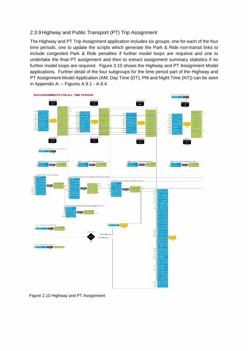
2.3.9 Highway and Public Transport (PT) Trip Assignment
The Highway and PT Trip Assignment application includes six groups; one for each of the four
time periods, one to update the scripts which generate the Park & Ride non-transit links to
include congested Park & Ride penalties if further model loops are required and one to
undertake the final PT assignment and then to extract assignment summary statistics if no
further model loops are required. Figure 3.10 shows the Highway and PT Assignment Model
applications. Further detail of the four subgroups for the time period part of the Highway and
PT Assignment Model Application (AM, Day Time (DT), PM and Night Time (NT)) can be seen
in Appendix A: – Figures A.9.1 - A.9.4.
Figure 2.10 Highway and PT Assignment
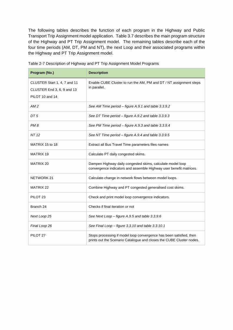
The following tables describes the function of each program in the Highway and Public
Transport Trip Assignment model application. Table 3.7 describes the main program structure
of the Highway and PT Trip Assignment model. The remaining tables describe each of the
four time periods (AM, DT, PM and NT), the next Loop and their associated programs within
the Highway and PT Trip Assignment model.
Program (No.) Description
CLUSTER Start 1, 4, 7 and 11
CLUSTER End 3, 6, 9 and 13
PILOT 10 and 14
Enable CUBE Cluster to run the AM, PM and DT / NT assignment steps
in parallel.
AM 2 See AM Time period – figure A.9.1 and table 3.3.9.2
DT 5 See DT Time period – figure A.9.2 and table 3.3.9.3
PM 8 See PM Time period – figure A.9.3 and table 3.3.9.4
NT 12 See NT Time period – figure A.9.4 and table 3.3.9.5
MATRIX 15 to 18 Extract all Bus Travel Time parameters files names
MATRIX 19 Calculate PT daily congested skims.
MATRIX 20 Dampen Highway daily congested skims, calculate model loop
convergence indicators and assemble Highway user benefit matrices.
NETWORK 21 Calculate change in network flows between model loops.
MATRIX 22 Combine Highway and PT congested generalised cost skims.
PILOT 23 Check and print model loop convergence indicators.
Branch 24 Checks if final iteration or not
Next Loop 25 See Next Loop – figure A.9.5 and table 3.3.9.6
Final Loop 26 See Final Loop – figure 3.3.10 and table 3.3.10.1
PILOT 27 Stops processing if model loop convergence has been satisfied, then
prints out the Scenario Catalogue and closes the CUBE Cluster nodes.
Table 2-7 Description of Highway and PT Trip Assignment Model Programs
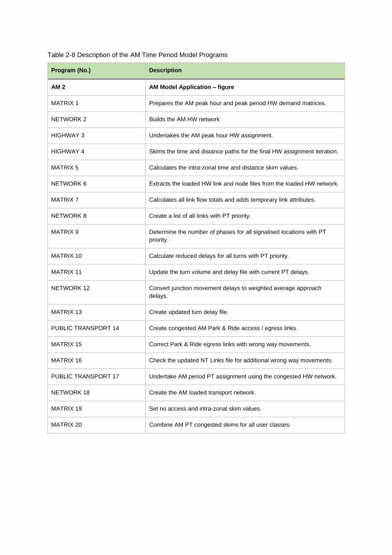
Program (No.) Description
AM 2 AM Model Application – figure
MATRIX 1 Prepares the AM peak hour and peak period HW demand matrices.
NETWORK 2 Builds the AM HW network
HIGHWAY 3 Undertakes the AM peak hour HW assignment.
HIGHWAY 4 Skims the time and distance paths for the final HW assignment iteration.
MATRIX 5 Calculates the intra-zonal time and distance skim values.
NETWORK 6 Extracts the loaded HW link and node files from the loaded HW network.
MATRIX 7 Calculates all link flow totals and adds temporary link attributes.
NETWORK 8 Create a list of all links with PT priority.
MATRIX 9 Determine the number of phases for all signalised locations with PT
priority.
MATRIX 10 Calculate reduced delays for all turns with PT priority.
MATRIX 11 Update the turn volume and delay file with current PT delays.
NETWORK 12 Convert junction movement delays to weighted average approach
delays.
MATRIX 13 Create updated turn delay file.
PUBLIC TRANSPORT 14 Create congested AM Park & Ride access / egress links.
MATRIX 15 Correct Park & Ride egress links with wrong way movements.
MATRIX 16 Check the updated NT Links file for additional wrong way movements.
PUBLIC TRANSPORT 17 Undertake AM period PT assignment using the congested HW network.
NETWORK 18 Create the AM loaded transport network.
MATRIX 19 Set no access and intra-zonal skim values.
MATRIX 20 Combine AM PT congested skims for all user classes.
Table 2-8 Description of the AM Time Period Model Programs
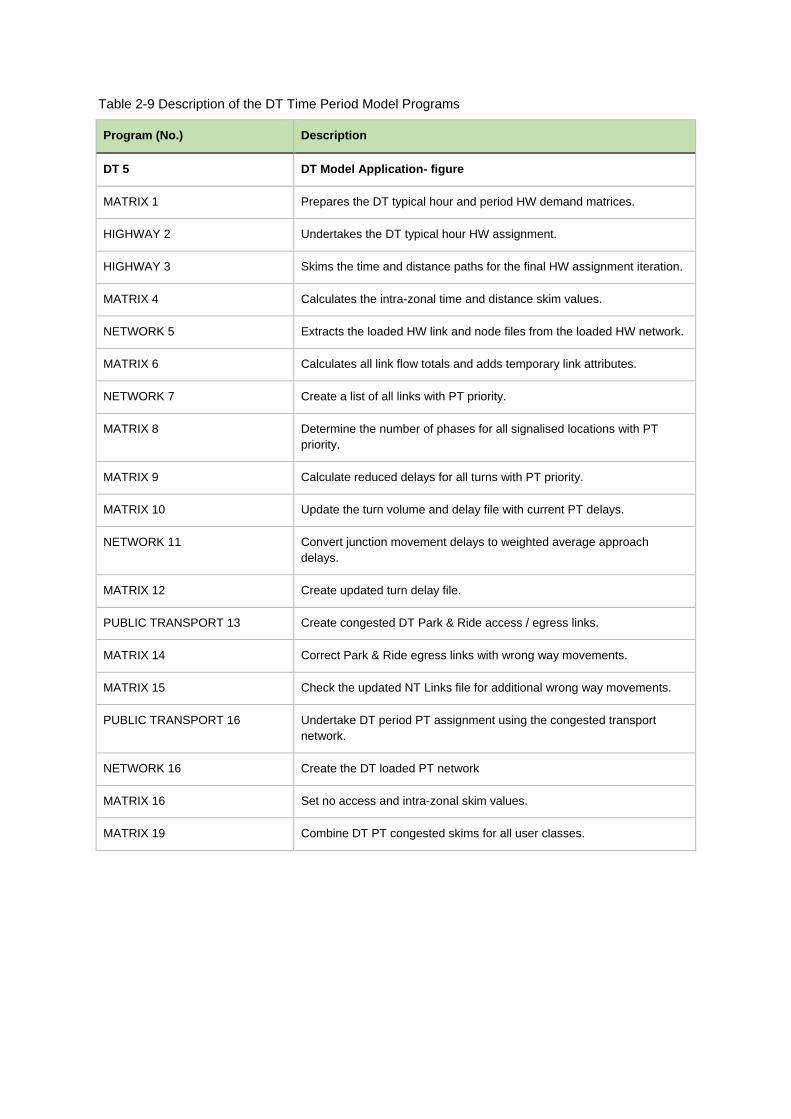
Program (No.) Description
DT 5 DT Model Application- figure
MATRIX 1 Prepares the DT typical hour and period HW demand matrices.
HIGHWAY 2 Undertakes the DT typical hour HW assignment.
HIGHWAY 3 Skims the time and distance paths for the final HW assignment iteration.
MATRIX 4 Calculates the intra-zonal time and distance skim values.
NETWORK 5 Extracts the loaded HW link and node files from the loaded HW network.
MATRIX 6 Calculates all link flow totals and adds temporary link attributes.
NETWORK 7 Create a list of all links with PT priority.
MATRIX 8 Determine the number of phases for all signalised locations with PT
priority.
MATRIX 9 Calculate reduced delays for all turns with PT priority.
MATRIX 10 Update the turn volume and delay file with current PT delays.
NETWORK 11 Convert junction movement delays to weighted average approach
delays.
MATRIX 12 Create updated turn delay file.
PUBLIC TRANSPORT 13 Create congested DT Park & Ride access / egress links.
MATRIX 14 Correct Park & Ride egress links with wrong way movements.
MATRIX 15 Check the updated NT Links file for additional wrong way movements.
PUBLIC TRANSPORT 16 Undertake DT period PT assignment using the congested transport
network.
NETWORK 16 Create the DT loaded PT network
MATRIX 16 Set no access and intra-zonal skim values.
MATRIX 19 Combine DT PT congested skims for all user classes.
Table 2-9 Description of the DT Time Period Model Programs
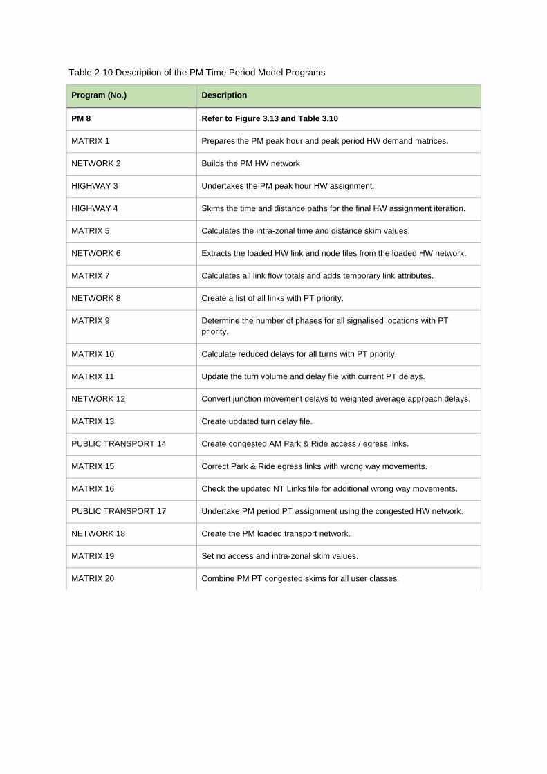
Table 2-10 Description of the PM Time Period Model Programs
Program (No.) Description
PM 8 Refer to Figure 3.13 and Table 3.10
MATRIX 1 Prepares the PM peak hour and peak period HW demand matrices.
NETWORK 2 Builds the PM HW network
HIGHWAY 3 Undertakes the PM peak hour HW assignment.
HIGHWAY 4 Skims the time and distance paths for the final HW assignment iteration.
MATRIX 5 Calculates the intra-zonal time and distance skim values.
NETWORK 6 Extracts the loaded HW link and node files from the loaded HW network.
MATRIX 7 Calculates all link flow totals and adds temporary link attributes.
NETWORK 8 Create a list of all links with PT priority.
MATRIX 9 Determine the number of phases for all signalised locations with PT
priority.
MATRIX 10 Calculate reduced delays for all turns with PT priority.
MATRIX 11 Update the turn volume and delay file with current PT delays.
NETWORK 12 Convert junction movement delays to weighted average approach delays.
MATRIX 13 Create updated turn delay file.
PUBLIC TRANSPORT 14 Create congested AM Park & Ride access / egress links.
MATRIX 15 Correct Park & Ride egress links with wrong way movements.
MATRIX 16 Check the updated NT Links file for additional wrong way movements.
PUBLIC TRANSPORT 17 Undertake PM period PT assignment using the congested HW network.
NETWORK 18 Create the PM loaded transport network.
MATRIX 19 Set no access and intra-zonal skim values.
MATRIX 20 Combine PM PT congested skims for all user classes.
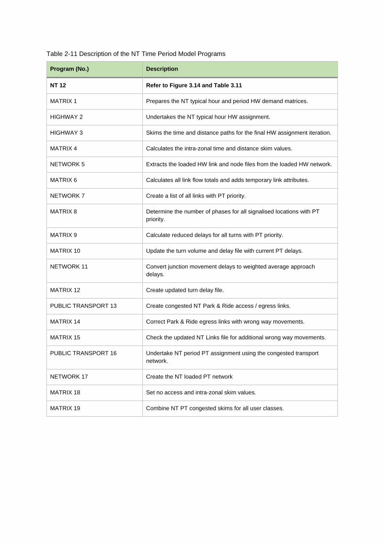
Program (No.) Description
NT 12 Refer to Figure 3.14 and Table 3.11
MATRIX 1 Prepares the NT typical hour and period HW demand matrices.
HIGHWAY 2 Undertakes the NT typical hour HW assignment.
HIGHWAY 3 Skims the time and distance paths for the final HW assignment iteration.
MATRIX 4 Calculates the intra-zonal time and distance skim values.
NETWORK 5 Extracts the loaded HW link and node files from the loaded HW network.
MATRIX 6 Calculates all link flow totals and adds temporary link attributes.
NETWORK 7 Create a list of all links with PT priority.
MATRIX 8 Determine the number of phases for all signalised locations with PT
priority.
MATRIX 9 Calculate reduced delays for all turns with PT priority.
MATRIX 10 Update the turn volume and delay file with current PT delays.
NETWORK 11 Convert junction movement delays to weighted average approach
delays.
MATRIX 12 Create updated turn delay file.
PUBLIC TRANSPORT 13 Create congested NT Park & Ride access / egress links.
MATRIX 14 Correct Park & Ride egress links with wrong way movements.
MATRIX 15 Check the updated NT Links file for additional wrong way movements.
PUBLIC TRANSPORT 16 Undertake NT period PT assignment using the congested transport
network.
NETWORK 17 Create the NT loaded PT network
MATRIX 18 Set no access and intra-zonal skim values.
MATRIX 19 Combine NT PT congested skims for all user classes.
Table 2-11 Description of the NT Time Period Model Programs
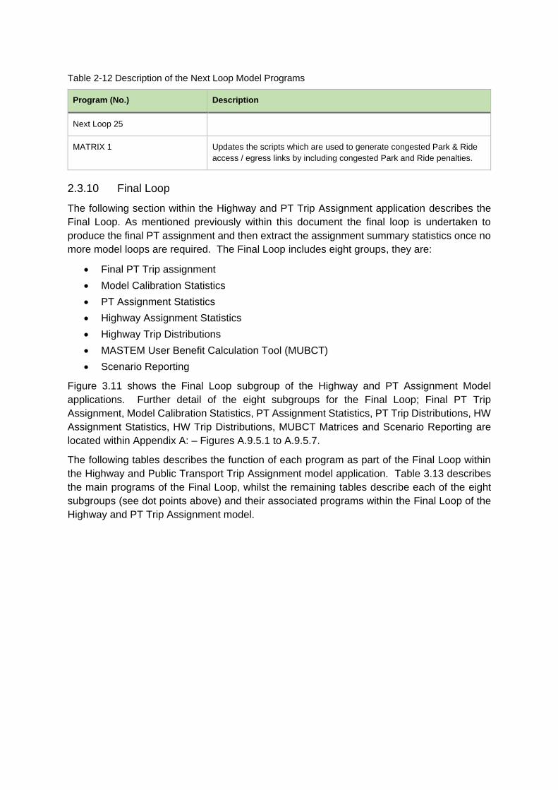
Program (No.) Description
Next Loop 25
MATRIX 1 Updates the scripts which are used to generate congested Park & Ride
access / egress links by including congested Park and Ride penalties.
2.3.10 Final Loop
The following section within the Highway and PT Trip Assignment application describes the
Final Loop. As mentioned previously within this document the final loop is undertaken to
produce the final PT assignment and then extract the assignment summary statistics once no
more model loops are required. The Final Loop includes eight groups, they are:
Final PT Trip assignment
Model Calibration Statistics
PT Assignment Statistics
Highway Assignment Statistics
Highway Trip Distributions
MASTEM User Benefit Calculation Tool (MUBCT)
Scenario Reporting
Figure 3.11 shows the Final Loop subgroup of the Highway and PT Assignment Model
applications. Further detail of the eight subgroups for the Final Loop; Final PT Trip
Assignment, Model Calibration Statistics, PT Assignment Statistics, PT Trip Distributions, HW
Assignment Statistics, HW Trip Distributions, MUBCT Matrices and Scenario Reporting are
located within Appendix A: – Figures A.9.5.1 to A.9.5.7.
The following tables describes the function of each program as part of the Final Loop within
the Highway and Public Transport Trip Assignment model application. Table 3.13 describes
the main programs of the Final Loop, whilst the remaining tables describe each of the eight
subgroups (see dot points above) and their associated programs within the Final Loop of the
Highway and PT Trip Assignment model.
Table 2-12 Description of the Next Loop Model Programs
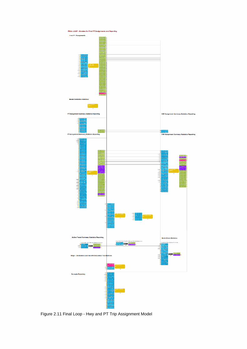
Figure 2.11 Final Loop - Hwy and PT Trip Assignment Model
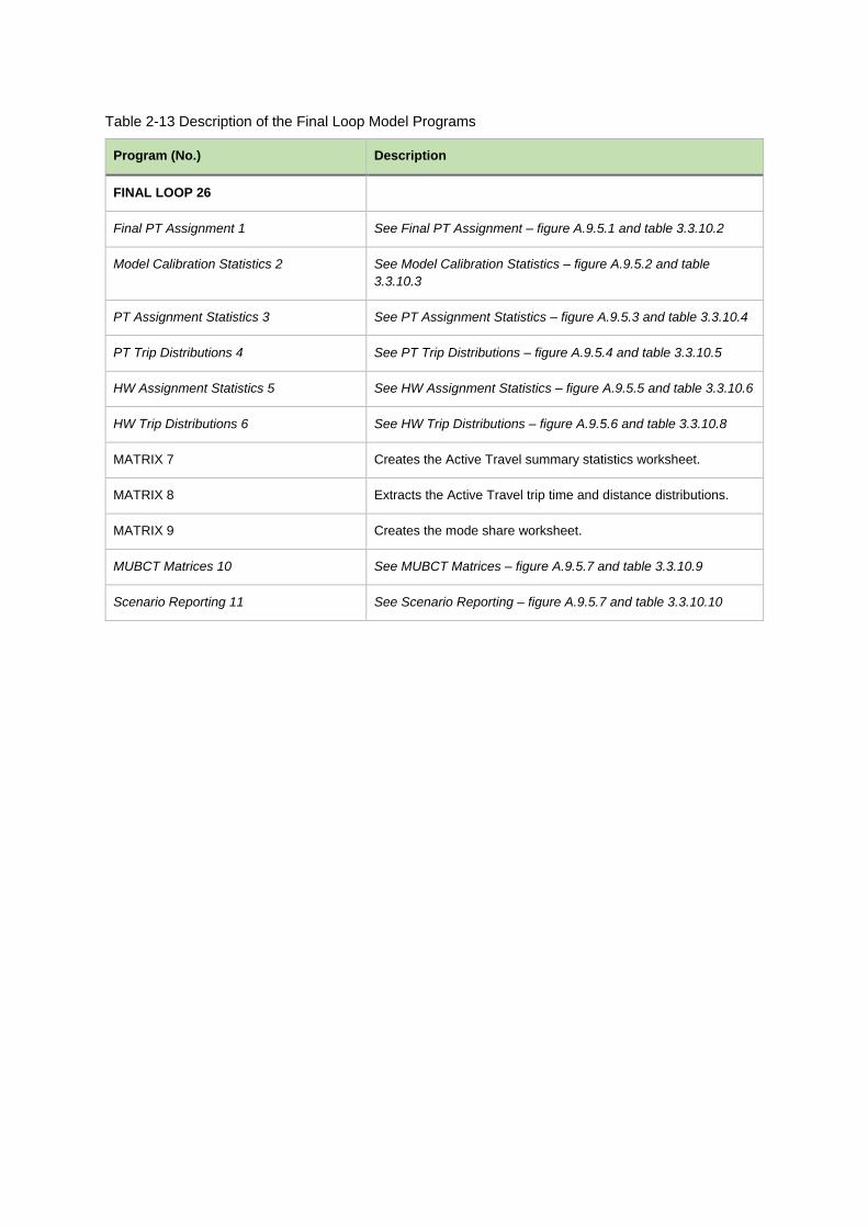
Program (No.) Description
FINAL LOOP 26
Final PT Assignment 1 See Final PT Assignment – figure A.9.5.1 and table 3.3.10.2
Model Calibration Statistics 2 See Model Calibration Statistics – figure A.9.5.2 and table
3.3.10.3
PT Assignment Statistics 3 See PT Assignment Statistics – figure A.9.5.3 and table 3.3.10.4
PT Trip Distributions 4 See PT Trip Distributions – figure A.9.5.4 and table 3.3.10.5
HW Assignment Statistics 5 See HW Assignment Statistics – figure A.9.5.5 and table 3.3.10.6
HW Trip Distributions 6 See HW Trip Distributions – figure A.9.5.6 and table 3.3.10.8
MATRIX 7 Creates the Active Travel summary statistics worksheet.
MATRIX 8 Extracts the Active Travel trip time and distance distributions.
MATRIX 9 Creates the mode share worksheet.
MUBCT Matrices 10 See MUBCT Matrices – figure A.9.5.7 and table 3.3.10.9
Scenario Reporting 11 See Scenario Reporting – figure A.9.5.7 and table 3.3.10.10
Table 2-13 Description of the Final Loop Model Programs
Program (No.) Description
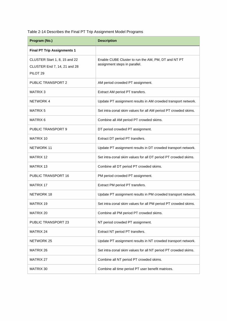
Final PT Trip Assignments 1
CLUSTER Start 1, 8, 15 and 22
CLUSTER End 7, 14, 21 and 28
PILOT 29
Enable CUBE Cluster to run the AM, PM, DT and NT PT
assignment steps in parallel.
PUBLIC TRANSPORT 2 AM period crowded PT assignment.
MATRIX 3 Extract AM period PT transfers.
NETWORK 4 Update PT assignment results in AM crowded transport network.
MATRIX 5 Set intra-zonal skim values for all AM period PT crowded skims.
MATRIX 6 Combine all AM period PT crowded skims.
PUBLIC TRANSPORT 9 DT period crowded PT assignment.
MATRIX 10 Extract DT period PT transfers.
NETWORK 11 Update PT assignment results in DT crowded transport network.
MATRIX 12 Set intra-zonal skim values for all DT period PT crowded skims.
MATRIX 13 Combine all DT period PT crowded skims.
PUBLIC TRANSPORT 16 PM period crowded PT assignment.
MATRIX 17 Extract PM period PT transfers.
NETWORK 18 Update PT assignment results in PM crowded transport network.
MATRIX 19 Set intra-zonal skim values for all PM period PT crowded skims.
MATRIX 20 Combine all PM period PT crowded skims.
PUBLIC TRANSPORT 23 NT period crowded PT assignment.
MATRIX 24 Extract NT period PT transfers.
NETWORK 25 Update PT assignment results in NT crowded transport network.
MATRIX 26 Set intra-zonal skim values for all NT period PT crowded skims.
MATRIX 27 Combine all NT period PT crowded skims.
MATRIX 30 Combine all time period PT user benefit matrices.
Table 2-14 Describes the Final PT Trip Assignment Model Programs
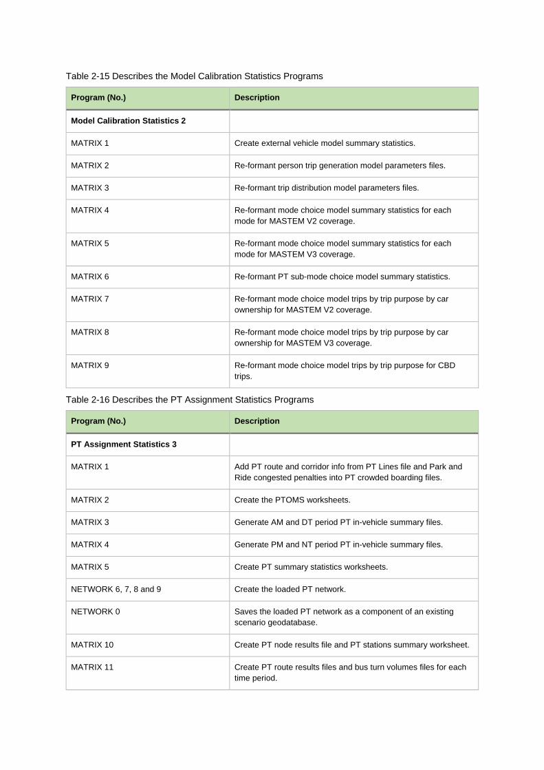
Program (No.) Description
Model Calibration Statistics 2
MATRIX 1 Create external vehicle model summary statistics.
MATRIX 2 Re-formant person trip generation model parameters files.
MATRIX 3 Re-formant trip distribution model parameters files.
MATRIX 4 Re-formant mode choice model summary statistics for each
mode for MASTEM V2 coverage.
MATRIX 5 Re-formant mode choice model summary statistics for each
mode for MASTEM V3 coverage.
MATRIX 6 Re-formant PT sub-mode choice model summary statistics.
MATRIX 7 Re-formant mode choice model trips by trip purpose by car
ownership for MASTEM V2 coverage.
MATRIX 8 Re-formant mode choice model trips by trip purpose by car
ownership for MASTEM V3 coverage.
MATRIX 9 Re-formant mode choice model trips by trip purpose for CBD
trips.
Program (No.) Description
PT Assignment Statistics 3
MATRIX 1 Add PT route and corridor info from PT Lines file and Park and
Ride congested penalties into PT crowded boarding files.
MATRIX 2 Create the PTOMS worksheets.
MATRIX 3 Generate AM and DT period PT in-vehicle summary files.
MATRIX 4 Generate PM and NT period PT in-vehicle summary files.
MATRIX 5 Create PT summary statistics worksheets.
NETWORK 6, 7, 8 and 9 Create the loaded PT network.
NETWORK 0 Saves the loaded PT network as a component of an existing
scenario geodatabase.
MATRIX 10 Create PT node results file and PT stations summary worksheet.
MATRIX 11 Create PT route results files and bus turn volumes files for each
time period.
Table 2-15 Describes the Model Calibration Statistics Programs
Table 2-16 Describes the PT Assignment Statistics Programs
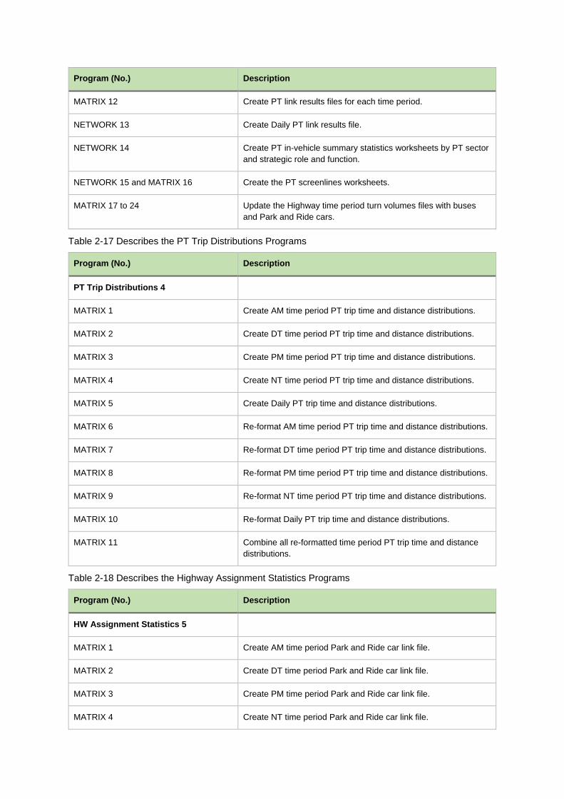
Program (No.) Description
MATRIX 12 Create PT link results files for each time period.
NETWORK 13 Create Daily PT link results file.
NETWORK 14 Create PT in-vehicle summary statistics worksheets by PT sector
and strategic role and function.
NETWORK 15 and MATRIX 16 Create the PT screenlines worksheets.
MATRIX 17 to 24 Update the Highway time period turn volumes files with buses
and Park and Ride cars.
Program (No.) Description
PT Trip Distributions 4
MATRIX 1 Create AM time period PT trip time and distance distributions.
MATRIX 2 Create DT time period PT trip time and distance distributions.
MATRIX 3 Create PM time period PT trip time and distance distributions.
MATRIX 4 Create NT time period PT trip time and distance distributions.
MATRIX 5 Create Daily PT trip time and distance distributions.
MATRIX 6 Re-format AM time period PT trip time and distance distributions.
MATRIX 7 Re-format DT time period PT trip time and distance distributions.
MATRIX 8 Re-format PM time period PT trip time and distance distributions.
MATRIX 9 Re-format NT time period PT trip time and distance distributions.
MATRIX 10 Re-format Daily PT trip time and distance distributions.
MATRIX 11 Combine all re-formatted time period PT trip time and distance
distributions.
Program (No.) Description
HW Assignment Statistics 5
MATRIX 1 Create AM time period Park and Ride car link file.
MATRIX 2 Create DT time period Park and Ride car link file.
MATRIX 3 Create PM time period Park and Ride car link file.
MATRIX 4 Create NT time period Park and Ride car link file.
Table 2-17 Describes the PT Trip Distributions Programs
Table 2-18 Describes the Highway Assignment Statistics Programs
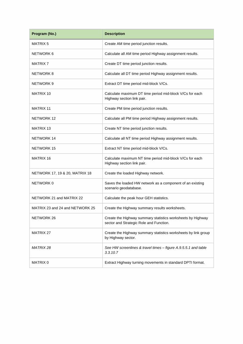
Program (No.) Description
MATRIX 5 Create AM time period junction results.
NETWORK 6 Calculate all AM time period Highway assignment results.
MATRIX 7 Create DT time period junction results.
NETWORK 8 Calculate all DT time period Highway assignment results.
NETWORK 9 Extract DT time period mid-block V/Cs.
MATRIX 10 Calculate maximum DT time period mid-block V/Cs for each
Highway section link pair.
MATRIX 11 Create PM time period junction results.
NETWORK 12 Calculate all PM time period Highway assignment results.
MATRIX 13 Create NT time period junction results.
NETWORK 14 Calculate all NT time period Highway assignment results.
NETWORK 15 Extract NT time period mid-block V/Cs.
MATRIX 16 Calculate maximum NT time period mid-block V/Cs for each
Highway section link pair.
NETWORK 17, 19 & 20, MATRIX 18 Create the loaded Highway network.
NETWORK 0 Saves the loaded HW network as a component of an existing
scenario geodatabase.
NETWORK 21 and MATRIX 22 Calculate the peak hour GEH statistics.
MATRIX 23 and 24 and NETWORK 25 Create the Highway summary results worksheets.
NETWORK 26 Create the Highway summary statistics worksheets by Highway
sector and Strategic Role and Function.
MATRIX 27 Create the Highway summary statistics worksheets by link group
by Highway sector.
MATRIX 28 See HW screenlines & travel times – figure A.9.5.5.1 and table
3.3.10.7
MATRIX 0 Extract Highway turning movements in standard DPTI format.
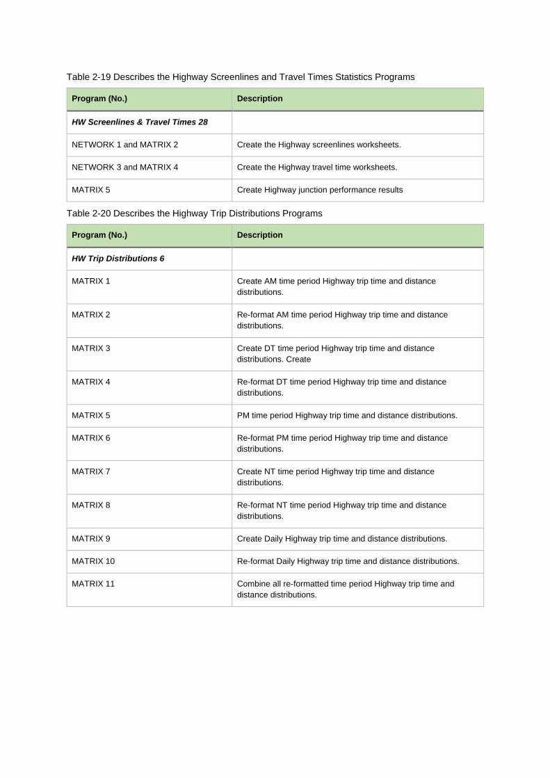
Program (No.) Description
HW Screenlines & Travel Times 28
NETWORK 1 and MATRIX 2 Create the Highway screenlines worksheets.
NETWORK 3 and MATRIX 4 Create the Highway travel time worksheets.
MATRIX 5 Create Highway junction performance results
Program (No.) Description
HW Trip Distributions 6
MATRIX 1 Create AM time period Highway trip time and distance
distributions.
MATRIX 2 Re-format AM time period Highway trip time and distance
distributions.
MATRIX 3 Create DT time period Highway trip time and distance
distributions. Create
MATRIX 4 Re-format DT time period Highway trip time and distance
distributions.
MATRIX 5 PM time period Highway trip time and distance distributions.
MATRIX 6 Re-format PM time period Highway trip time and distance
distributions.
MATRIX 7 Create NT time period Highway trip time and distance
distributions.
MATRIX 8 Re-format NT time period Highway trip time and distance
distributions.
MATRIX 9 Create Daily Highway trip time and distance distributions.
MATRIX 10 Re-format Daily Highway trip time and distance distributions.
MATRIX 11 Combine all re-formatted time period Highway trip time and
distance distributions.
Table 2-19 Describes the Highway Screenlines and Travel Times Statistics Programs
Table 2-20 Describes the Highway Trip Distributions Programs
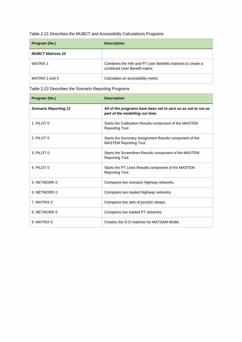
Program (No.) Description
MUBCT Matrices 10
MATRIX 1 Combines the HW and PT User Benefits matrices to create a
combined User Benefit matrix.
MATRIX 2 and 3 Calculates an accessibility metric
Program (No.) Description
Scenario Reporting 11 All of the programs have been set to zero so as not to run as
part of the modelling run time.
1. PILOT 0 Starts the Calibration Results component of the MASTEM
Reporting Tool.
2. PILOT 0 Starts the Summary Assignment Results component of the
MASTEM Reporting Tool.
3. PILOT 0 Starts the Screenlines Results component of the MASTEM
Reporting Tool.
4. PILOT 0 Starts the PT Lines Results component of the MASTEM
Reporting Tool.
5. NETWORK 0 Compares two scenario Highway networks.
6. NETWORK 0 Compares two loaded Highway networks.
7. MATRIX 0 Compares two sets of junction delays.
8. NETWORK 0 Compares two loaded PT networks.
9. MATRIX 0 Creates the O-D matrices for MATSAM Model.
Table 2-21 Describes the MUBCT and Accessibility Calculations Programs
Table 2-22 Describes the Scenario Reporting Programs
4.0 Model Inputs
4.1 Catalog Keys
Each model run is defined by a series of CUBE Catalog Keys. These keys have been
arranged in three groups:
General Model Parameters,
Highway Inputs, and
Public Transport Inputs.
All of the keys within each of these groups are described below in a graphical and tabular
format. (See Appendix B: for further detail of the Scenario Manager Catalog Key screens).
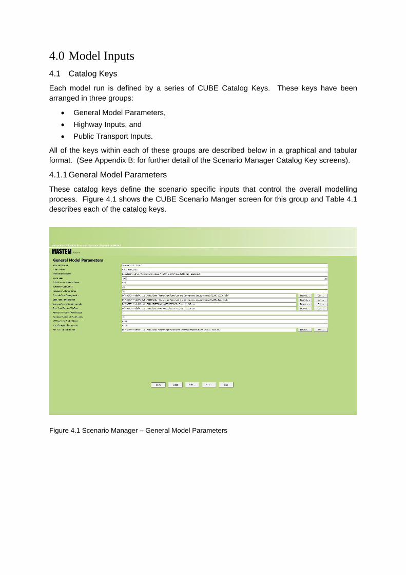
4.1.1 General Model Parameters
These catalog keys define the scenario specific inputs that control the overall modelling
process. Figure 4.1 shows the CUBE Scenario Manger screen for this group and Table 4.1
describes each of the catalog keys.
Figure 4.1 Scenario Manager – General Model Parameters
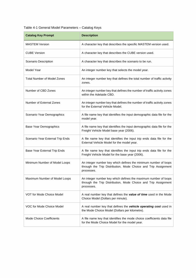
Catalog Key Prompt Description
MASTEM Version A character key that describes the specific MASTEM version used.
CUBE Version A character key that describes the CUBE version used.
Scenario Description A character key that describes the scenario to be run.
Model Year An integer number key that selects the model year.
Total Number of Model Zones An integer number key that defines the total number of traffic activity
zones.
Number of CBD Zones An integer number key that defines the number of traffic activity zones
within the Adelaide CBD.
Number of External Zones An integer number key that defines the number of traffic activity zones
for the External Vehicle Model.
Scenario Year Demographics A file name key that identifies the input demographic data file for the
model year.
Base Year Demographics A file name key that identifies the input demographic data file for the
Freight Vehicle Model base year (2006).
Scenario Year External Trip Ends A file name key that identifies the input trip ends data file for the
External Vehicle Model for the model year.
Base Year External Trip Ends A file name key that identifies the input trip ends data file for the
Freight Vehicle Model for the base year (2006).
Minimum Number of Model Loops An integer number key which defines the minimum number of loops
through the Trip Distribution, Mode Choice and Trip Assignment
processes.
Maximum Number of Model Loops An integer number key which defines the maximum number of loops
through the Trip Distribution, Mode Choice and Trip Assignment
processes.
VOT for Mode Choice Model A real number key that defines the value of time used in the Mode
Choice Model (Dollars per minute).
VOC for Mode Choice Model A real number key that defines the vehicle operating cost used in
the Mode Choice Model (Dollars per kilometre).
Mode Choice Coefficients A file name key that identifies the mode choice coefficients data file
for the Mode Choice Model for the model year.
Table 4-1 General Model Parameters – Catalog Keys
4.1.2 Highway Inputs
These catalog keys define the scenario inputs required for Highway assignments. Figure 4.2
shows the CUBE Scenario Manger screen for this group and Table 4.2 describes each of the
catalog keys.
Figure 4.2 Scenario Manager - Highway Inputs

Catalog Key Prompt Description
Input Foundation Network A file name key that identifies the input Foundation Network. This
may be a *.NET, *.MDB or *.GDB. Table A.1 of Appendix A describes
the Foundation Network node and link attributes.
Foundation Network Shape File A file name key that defines the shape file associated with the
Foundation Network. All links except for zone connectors and walk
only links should have a defined shape. The length of each link
should match the ArcGIS calculated length rather than the CUBE
calculated length.
DT and NT Junction File A file name key that identifies the input junction file (*.IND) for the DT
and NT time.
AM Junction File A file name key that identifies the input junction file (*.IND) for the AM
time period.
PM Junction File A file name key that identifies the input junction file (*.IND) for the PM
time period.
DT and NT Turn Penalty File A file name key that identifies the input turn penalty file (*.PEN) for
the DT and NT time periods.
AM Turn Penalty File A file name key that identifies the input turn penalty file (*.PEN) for
the AM time period.
PM Turn Penalty File A file name key that identifies the input turn penalty file (*.PEN) for
the PM time period.
Time Factor for Highway Assignment A real number key that defines the time cost factor for path building
paths during the Highway assignment process.
Distance Factor for Cars in Highway
Assignment
A real number key that contains the distance cost factor for building
paths for cars during the Highway assignment process.
Distance Factor for Trucks in Highway
Assignment
A real number key that contains the distance cost factor for building
paths for trucks during the Highway assignment process.
Car Parking Cost File A file name key that identifies the car parking cost file which defines
the cost of parking for work and non-work purposes.
Vehicle or PCU Assignment A character key selected by radio buttons that determines whether a
“Vehicle” or “Passenger Car Unit” (PCU) equivalent Highway
assignment is undertaken.
Table 4-2 Highway Inputs - Catalog Keys
4.1.3 Public Transport Inputs
These catalog keys define the scenario inputs required for Public Transport assignments.
Figure 4.3 shows the CUBE Scenario Manger screen for this group and Table 4.3 describes
each of the catalog keys.
Figure 4.3 Scenario Manager - Public Transport Inputs
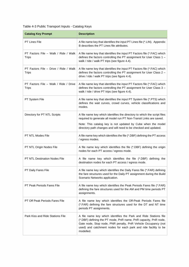
Catalog Key Prompt Description
PT Lines File A file name key that identifies the input PT Lines file (*.LIN). Appendix
B describes the PT Lines file attributes.
PT Factors File – Walk / Ride / Walk
Trips
A file name key that identifies the input PT Factors file (*.FAC) which
defines the factors controlling the PT assignment for User Class 1 –
walk / ride / walk PT trips (see figure 4.4).
PT Factors File – Drive / Ride / Walk
Trips
A file name key that identifies the input PT Factors file (*.FAC) which
defines the factors controlling the PT assignment for User Class 2 –
drive / ride / walk PT trips (see figure 4.4).
PT Factors File – Walk / Ride / Drive
Trips
A file name key that identifies the input PT Factors file (*.FAC) which
defines the factors controlling the PT assignment for User Class 3 –
walk / ride / drive PT trips (see figure 4.4).
PT System File A file name key that identifies the input PT System file (*.PTS) which
defines the wait curves, crowd curves, vehicle classifications and
modes.
Directory for PT NTL Scripts A file name key which identifies the directory to which the script files
required to generate all model run PT Non-Transit Links are saved.
Note: This catalog key is not updated by Cube when the model
directory path changes and will need to be checked and updated.
PT NTL Modes File A file name key which identifies the file (*.DBF) defining the PT access
/ egress modes.
PT NTL Origin Nodes File A file name key which identifies the file (*.DBF) defining the origin
nodes for each PT access / egress mode.
PT NTL Destination Nodes File A file name key which identifies the file (*.DBF) defining the
destination nodes for each PT access / egress mode.
PT Daily Fares File A file name key which identifies the Daily Fares file (*.FAR) defining
the fare structures used for the Daily PT assignment during the Build
Scenario Networks application.
PT Peak Periods Fares File A file name key which identifies the Peak Periods Fares file (*.FAR)
defining the fare structures used for the AM and PM time periods PT
assignments.
PT Off Peak Periods Fares File A file name key which identifies the Off-Peak Periods Fares file
(*.FAR) defining the fare structures used for the DT and NT time
periods PT assignments.
Park Kiss and Ride Stations File A file name key which identifies the Park and Ride Stations file
(*.DBF) defining the PT mode, PnR name, PnR capacity, PnR node,
Gate node, Stop node, PNR penalty, PnR Vehicle Occupancy (not
used) and catchment nodes for each park and ride facility to be
modelled.
Table 4-3 Public Transport Inputs - Catalog Keys

Catalog Key Prompt Description
Park Kiss and Ride Vehicle Occupancy
File
A file name key which identifies the Park and Ride Vehicle Occupancy
file (*.DBF) defining the PnR Vehicle Occupancy for each time period.
Note that the values defined in this file are used rather than the values
defined in the Park Kiss and Ride Stations file.
PT Interchanges File A file name key which identifies the PT Interchanges file (*.DBF)
defining the PT interchange nodes with a medium and high level of
connectivity.
Run Crowding Model in Final PT
Assignments Only
A Boolean key defined by a check box which activates the Crowding
Model in the final PT assignments.
Run Crowding Model Inside Model Loop A Boolean key defined by a check box which activates the Crowding
Model in the PT assignments during the model loop process.
Maximum Number of Crowding Models
Iterations
An integer key that defines the maximum number of iterations for the
PT crowding model.
User Class 1 allows only walk-in and walk-out modes;
User Class 2 allows only drive-I (drive access) mode; and
User Class 3 allows only drive-out (drive egress) mode.
Figure 4.4 Access modes applicable for three public transport user classes
5.0 Developing/Running Scenarios
5.1 Overview
In developing and running a scenario in MASTEM there are a number of areas that need to
be defined and checked depending on the type of scenario being tested – such as a new road
link/capacity change; new public transport line (bus, tram or train).
Before any modelling work occurs there needs to be a clear picture of the relationship between
the base case and project options within the business case. Meaning that if the base case to
project case testing is to be used for a transport model outcome (e.g. testing different policy
options) or an economic model (e.g. providing a benefit to cost output) or both is required.
As with any strategic model and scenario testing there are a number of variables that can be
changed/developed for testing – these are described below.
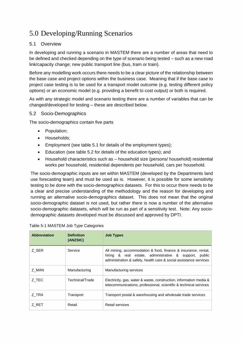
5.2 Socio-Demographics
The socio-demographics contain five parts
Population;
Households;
Employment (see table 5.1 for details of the employment types);
Education (see table 5.2 for details of the education types); and
Household characteristics such as – household size (persons/ household) residential
works per household, residential dependents per household, cars per household.
The socio-demographic inputs are set within MASTEM (developed by the Departments land
use forecasting team) and must be used as is. However, it is possible for some sensitivity
testing to be done with the socio-demographics datasets. For this to occur there needs to be
a clear and precise understanding of the methodology and the reason for developing and
running an alternative socio-demographics dataset. This does not mean that the original
socio-demographic dataset is not used, but rather there is now a number of the alternative
socio-demographic datasets, which will be run as part of a sensitivity test. Note: Any socio-
demographic datasets developed must be discussed and approved by DPTI.
Abbreviation Definition
(ANZSIC)
Job Types
Z_SER Service All mining, accommodation & food, finance & insurance, rental,
hiring & real estate, administrative & support, public
administration & safety, health care & social assistance services
Z_MAN Manufacturing Manufacturing services
Z_TEC Technical/Trade Electricity, gas, water & waste, construction, information media &
telecommunications, professional, scientific & technical services
Z_TRA Transport Transport postal & warehousing and wholesale trade services
Z_RET Retail Retail services
Table 5-1 MASTEM Job Type Categories
Abbreviation Definition
(ANZSIC)
Job Types
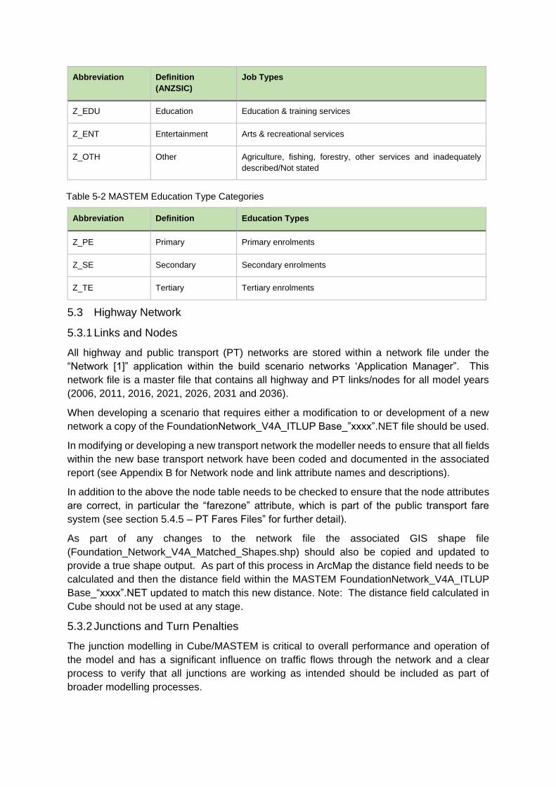
Z_EDU Education Education & training services
Z_ENT Entertainment Arts & recreational services
Z_OTH Other Agriculture, fishing, forestry, other services and inadequately
described/Not stated
Abbreviation Definition Education Types
Z_PE Primary Primary enrolments
Z_SE Secondary Secondary enrolments
Z_TE Tertiary Tertiary enrolments
5.3 Highway Network
5.3.1 Links and Nodes
All highway and public transport (PT) networks are stored within a network file under the
“Network [1]” application within the build scenario networks ‘Application Manager”. This
network file is a master file that contains all highway and PT links/nodes for all model years
(2006, 2011, 2016, 2021, 2026, 2031 and 2036).
When developing a scenario that requires either a modification to or development of a new
network a copy of the FoundationNetwork_V4A_ITLUP Base_”xxxx”.NET file should be used.
In modifying or developing a new transport network the modeller needs to ensure that all fields
within the new base transport network have been coded and documented in the associated
report (see Appendix B for Network node and link attribute names and descriptions).
In addition to the above the node table needs to be checked to ensure that the node attributes
are correct, in particular the “farezone” attribute, which is part of the public transport fare
system (see section 5.4.5 – PT Fares Files” for further detail).
As part of any changes to the network file the associated GIS shape file
(Foundation_Network_V4A_Matched_Shapes.shp) should also be copied and updated to
provide a true shape output. As part of this process in ArcMap the distance field needs to be
calculated and then the distance field within the MASTEM FoundationNetwork_V4A_ITLUP
Base_“xxxx”.NET updated to match this new distance. Note: The distance field calculated in
Cube should not be used at any stage.
5.3.2 Junctions and Turn Penalties
The junction modelling in Cube/MASTEM is critical to overall performance and operation of
the model and has a significant influence on traffic flows through the network and a clear
process to verify that all junctions are working as intended should be included as part of
broader modelling processes.
Table 5-2 MASTEM Education Type Categories
The junction model within MASTEM should closely emulate SCATS performance, although
this will be limited to some extent by the limitations of the CUBE junction modelling. The
junction model should be robust under a range of possible scenarios / time periods in order to
minimise the effort required to effectively develop this critical component of the model. The
significant limitations imposed by the CUBE platform emphasises the need for a clearly
documented review / verification process as part of any modelling work.
There are two files that make up the junction modelling aspect within MASTEM. They are
{time period} Junction Files; and
{time period} Penalty Files
The Junction File describes the layout and operation of all signal controlled junctions within
MASTEM. A junction file exists for each time period and model year e.g. Time period - AM,
PM, Daily, Model years - 2006, 2011, 2016, 2021, 2026, 2031 and 2036. When developing a
new network, which either modifies existing or creates any new intersections the original
junction files need to be copied and saved as a new version for the scenario being testing. As
part of modifying / updating or creating a new junction description within the junction file a
description of the modifications / updates or additions needs to be included (see junction file
for details) and associated report. As outlined above, the same description – i.e. lane
arrangement, phasing etc. – should be used for the 3 time periods junction files for all relevant
model year’s dependent of the time frame of the change.
As outlined above, there is a requirement to check the performance of the signal controlled
junctions to determine whether or not any further changes need to be made to the operation
of any of the signal controlled junctions.
This checking is simplified by using the output files from the “Highway Junction Performance”
application (see matrix 5 under HW Assignment Statistics – HW Statistics & Travel Times)
within the model. The preferred method is to run both the Foundation Network scenario and
the alternative scenario and compare the two Highway Junction Performance outputs. If
changes are required, they should be made to the junction files which can be tested by running
relevant time period assignment application steps. Note that the full model will need to be
rerun once a final set of junction files have been developed.
Turn penalty files may be used to ban movements or to add delay to specific movements.
Again, model outputs need to be checked to confirm that is the turn penalty files are working
as intended.
Further details of junction modelling requirements can be found in Appendix D.
5.3.3 Parking Costs
This input parking costs file contains parking charges at designation zones for work and non-
work purposes. These costs are for the full day and should be expressed as zonal averages
in cents, and in 2006 prices.
Values currently vary by zone and purpose:
Work: $5.55 to $9.05 (all day)
Non-work: $0.90 to $2.05 (1hr)
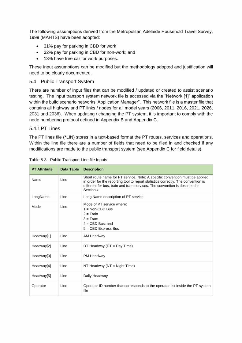
The following assumptions derived from the Metropolitan Adelaide Household Travel Survey,
1999 (MAHTS) have been adopted:
31% pay for parking in CBD for work
32% pay for parking in CBD for non-work; and
13% have free car for work purposes.
These input assumptions can be modified but the methodology adopted and justification will
need to be clearly documented.
5.4 Public Transport System
There are number of input files that can be modified / updated or created to assist scenario
testing. The input transport system network file is accessed via the “Network [1]” application
within the build scenario networks ‘Application Manager”. This network file is a master file that
contains all highway and PT links / nodes for all model years (2006, 2011, 2016, 2021, 2026,
2031 and 2036). When updating / changing the PT system, it is important to comply with the
node numbering protocol defined in Appendix B and Appendix C.
5.4.1 PT Lines
The PT lines file (*LIN) stores in a text-based format the PT routes, services and operations.
Within the line file there are a number of fields that need to be filed in and checked if any
modifications are made to the public transport system (see Appendix C for field details).
PT Attribute Data Table Description
Name Line Short route name for PT service. Note: A specific convention must be applied in order for the reporting tool to report statistics correctly. The convention is different for bus, train and tram services. The convention is described in Section x.
LongName Line Long Name description of PT service
Mode Line Mode of PT service where:
1 = Non-CBD Bus
2 = Train
3 = Tram
4 = CBD Bus; and
5 = CBD Express Bus
Headway[1] Line AM Headway
Headway[2] Line DT Headway (DT = Day Time)
Headway[3] Line PM Headway
Headway[4] Line NT Headway (NT = Night Time)
Headway[5] Line Daily Headway
Operator Line Operator ID number that corresponds to the operator list inside the PT system
file
Table 5-3 - Public Transport Line file Inputs
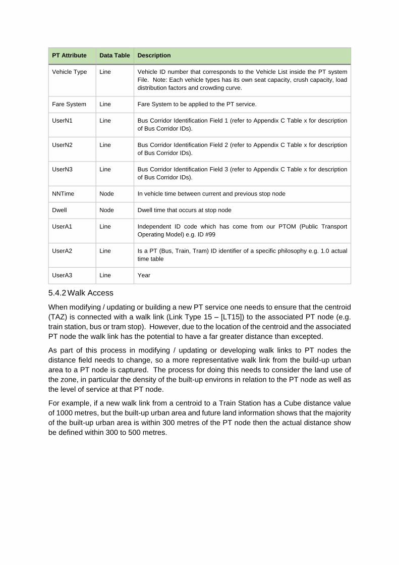
PT Attribute Data Table Description
Vehicle Type Line Vehicle ID number that corresponds to the Vehicle List inside the PT system
File. Note: Each vehicle types has its own seat capacity, crush capacity, load
distribution factors and crowding curve.
Fare System Line Fare System to be applied to the PT service.
UserN1 Line Bus Corridor Identification Field 1 (refer to Appendix C Table x for description
of Bus Corridor IDs).
UserN2 Line Bus Corridor Identification Field 2 (refer to Appendix C Table x for description
of Bus Corridor IDs).
UserN3 Line Bus Corridor Identification Field 3 (refer to Appendix C Table x for description
of Bus Corridor IDs).
NNTime Node In vehicle time between current and previous stop node
Dwell Node Dwell time that occurs at stop node
UserA1 Line Independent ID code which has come from our PTOM (Public Transport
Operating Model) e.g. ID #99
UserA2 Line Is a PT (Bus, Train, Tram) ID identifier of a specific philosophy e.g. 1.0 actual
time table
UserA3 Line Year
5.4.2 Walk Access
When modifying / updating or building a new PT service one needs to ensure that the centroid
(TAZ) is connected with a walk link (Link Type 15 – [LT15]) to the associated PT node (e.g.
train station, bus or tram stop). However, due to the location of the centroid and the associated
PT node the walk link has the potential to have a far greater distance than excepted.
As part of this process in modifying / updating or developing walk links to PT nodes the
distance field needs to change, so a more representative walk link from the build-up urban
area to a PT node is captured. The process for doing this needs to consider the land use of
the zone, in particular the density of the built-up environs in relation to the PT node as well as
the level of service at that PT node.
For example, if a new walk link from a centroid to a Train Station has a Cube distance value
of 1000 metres, but the built-up urban area and future land information shows that the majority
of the built-up urban area is within 300 metres of the PT node then the actual distance show
be defined within 300 to 500 metres.

5.4.3 PT Factors File
The PT factors file (*FAC) contains all the PT factor parameters for controlling the public
transport Walk user class assignment. There are 3 files for each model year - user classes:
UC1 = Walk/Ride/Walk trips
UC2 = Drive/Ride/Walk trips; and
UC3 = Walk/Ride/Drive trips
(See figure 4.4 for further detail)
Within these user class files contains a number of factors (see PTFactors_UC1_YYYY file in
MASTEM):
BRDPEN [1] = Boarding penalty is a mode specific boarding penalty in minutes
RUNFACTOR [1] = Run factor mode-specific weighting factor applied to transit in-
vehicle times and non-transit leg times.
WAITFACTOR [1] = Node-specific wait-time weighting factor, applied to nodes.
XFERPEN = Transit mode to transit mode transfer penalty, in minutes.
IWAITCURVE = Wait curve used to calculated the initial wait time for trips starting at
nodes specified.
XWAITCURVE = Wait-curve number used to calculate wait times for trips that involve
transfers to nodes specified.
5.4.4 PT System File
The PT system file (*PTS) stores wait curves, crowd curves, PT vehicle classifications and
mode definitions.
Figure 5.1 - Walk Link Distance for Built-Up Urban Area
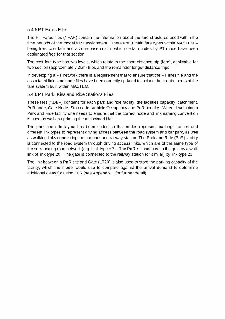
5.4.5 PT Fares Files
The PT Fares files (*.FAR) contain the information about the fare structures used within the
time periods of the model’s PT assignment. There are 3 main fare types within MASTEM –
being free, cost-fare and a zone-base cost in which certain nodes by PT mode have been
designated free for that section.
The cost-fare type has two levels, which relate to the short distance trip (fare), applicable for
two section (approximately 3km) trips and the remainder longer distance trips.
In developing a PT network there is a requirement that to ensure that the PT lines file and the
associated links and node files have been correctly updated to include the requirements of the
fare system built within MASTEM.
5.4.6 PT Park, Kiss and Ride Stations Files
These files (*.DBF) contains for each park and ride facility, the facilities capacity, catchment,
PnR node, Gate Node, Stop node, Vehicle Occupancy and PnR penalty. When developing a
Park and Ride facility one needs to ensure that the correct node and link naming convention
is used as well as updating the associated files.
The park and ride layout has been coded so that nodes represent parking facilities and
different link types to represent driving access between the road system and car park, as well
as walking links connecting the car park and railway station. The Park and Ride (PnR) facility
is connected to the road system through driving access links, which are of the same type of
the surrounding road network (e.g. Link type = 7). The PnR is connected to the gate by a walk
link of link type 20. The gate is connected to the railway station (or similar) by link type 21.
The link between a PnR site and Gate (LT20) is also used to store the parking capacity of the
facility, which the model would use to compare against the arrival demand to determine
additional delay for using PnR (see Appendix C for further detail).
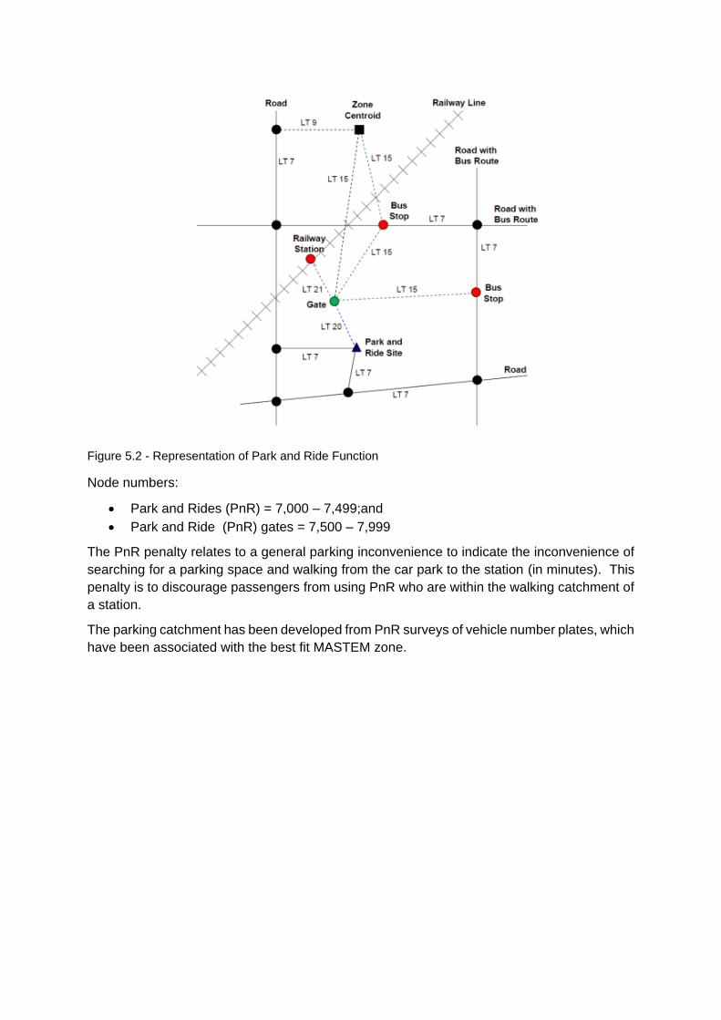
Node numbers:
Park and Rides (PnR) = 7,000 – 7,499;and
Park and Ride (PnR) gates = 7,500 – 7,999
The PnR penalty relates to a general parking inconvenience to indicate the inconvenience of
searching for a parking space and walking from the car park to the station (in minutes). This
penalty is to discourage passengers from using PnR who are within the walking catchment of
a station.
The parking catchment has been developed from PnR surveys of vehicle number plates, which
have been associated with the best fit MASTEM zone.
Figure 5.2 - Representation of Park and Ride Function
5.4.7 PT Interchanges File
The PT interchange priority file (*.DBF) contains a list of interchange nodes with a medium
and high level of connectivity. The list of interchange nodes must be sorted in ascending
order. This list has bus, train and tram interchange priorities and has a separate file for each
of the model years.
The level of connectivity defined relates to the transfer wait curve (XWC type).
The PT interchange type defined as follows:
1 = normal connection – transfer penalty: 5 minutes (within modes) – 7 minutes (between
modes); (the default)
2 = good connection – transfer penalty: 2.5 – 4.5 minutes; and
3 = excellent connection – transfer penalty: 0 – 2 minutes.
The normal interchange represents the existing interchange facilities. The excellent
connecting interchange would be reserved for future scenarios, where new interchanges
would be built or improved in such a way that there would be connecting, comfortable and
seamless transfers between services.
Since the transfer penalty is associated with mode, while transfer curves are associated with
the node, means that to model future interchange conditions by node level the 5 minute
transfer penalty has to be associated with the normal transfer wait curve, and the two other
transfer wait curves (good and excellent) have their own wait curves.
5.5 Public Transport priority
5.5.1 Bus Lanes
A bus lane facility that allows a bus to have its own lane during certain time periods. A bus
lane is represented in the network by using the link attribute:
BUS_LANE with the following codes:
1 = Bus Lane – All day
2 = Bus Lane – Peaks only
3 = Bus Lane – AM peak only
4 = Bus Lane – PM peak only; and
5 = Bus Lane – AM peak, Daytime, PM peak only
For the road links that have bus lanes, it is assumed the bus lane will operate at the free speed
as they do not have to interact with general traffic mix. In these cases, bus travel time is set
equal to the free flow travel time plus intersection delay.
5.5.2 Junction Priority
The highway assignment produces output turn penalty files that summarise the delay for each
movement at each intersection. These outputs can be linked into the PT module as an input
so that PT paths and in-vehicle time will consider the turn delay.
A link attribute, BUS_PRIORITY has been coded in the highway network to identify the
approaches having bus priority. In the situation where bus priority exists, the bus will
experience considerable less delay at the intersection compared to other vehicles. As soon
as a bus arrives at an intersection, it will be given priority to make its movement within the next
phase.
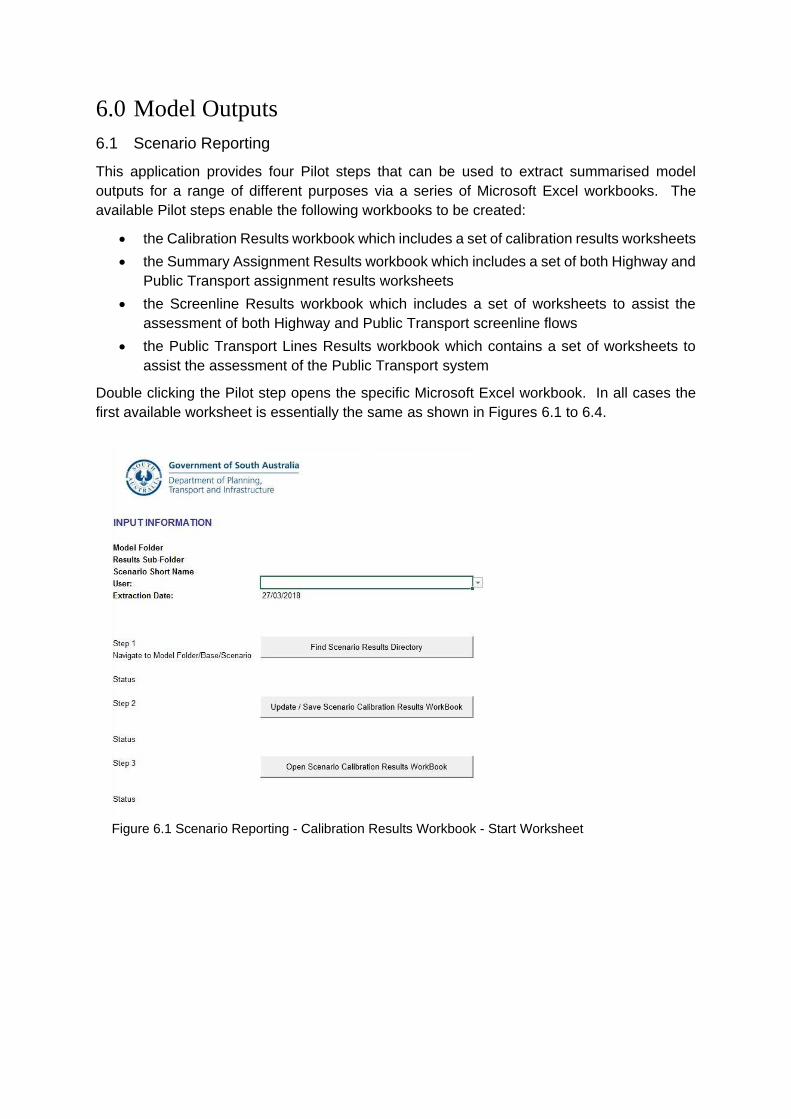
6.0 Model Outputs
6.1 Scenario Reporting
This application provides four Pilot steps that can be used to extract summarised model
outputs for a range of different purposes via a series of Microsoft Excel workbooks. The
available Pilot steps enable the following workbooks to be created:
the Calibration Results workbook which includes a set of calibration results worksheets
the Summary Assignment Results workbook which includes a set of both Highway and
Public Transport assignment results worksheets
the Screenline Results workbook which includes a set of worksheets to assist the
assessment of both Highway and Public Transport screenline flows
the Public Transport Lines Results workbook which contains a set of worksheets to
assist the assessment of the Public Transport system
Double clicking the Pilot step opens the specific Microsoft Excel workbook. In all cases the
first available worksheet is essentially the same as shown in Figures 6.1 to 6.4.
Figure 6.1 Scenario Reporting - Calibration Results Workbook - Start Worksheet
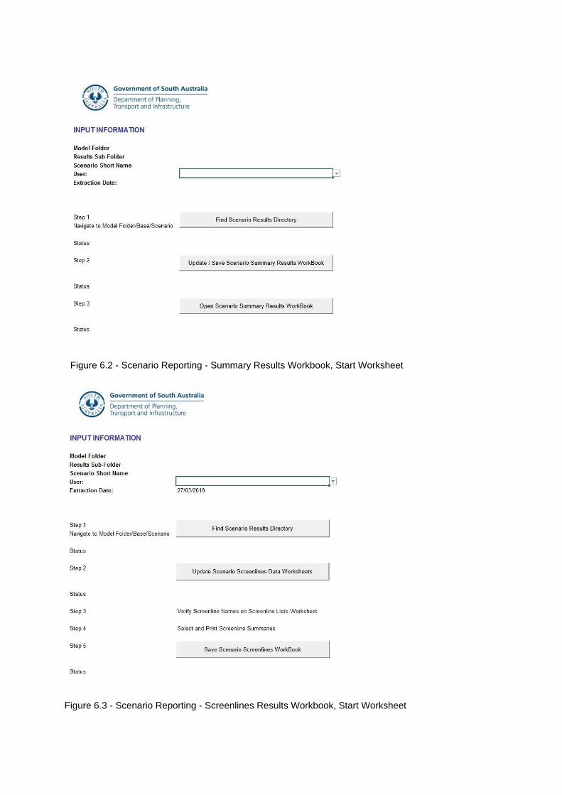
Figure 6.2 - Scenario Reporting - Summary Results Workbook, Start Worksheet
Figure 6.3 - Scenario Reporting - Screenlines Results Workbook, Start Worksheet
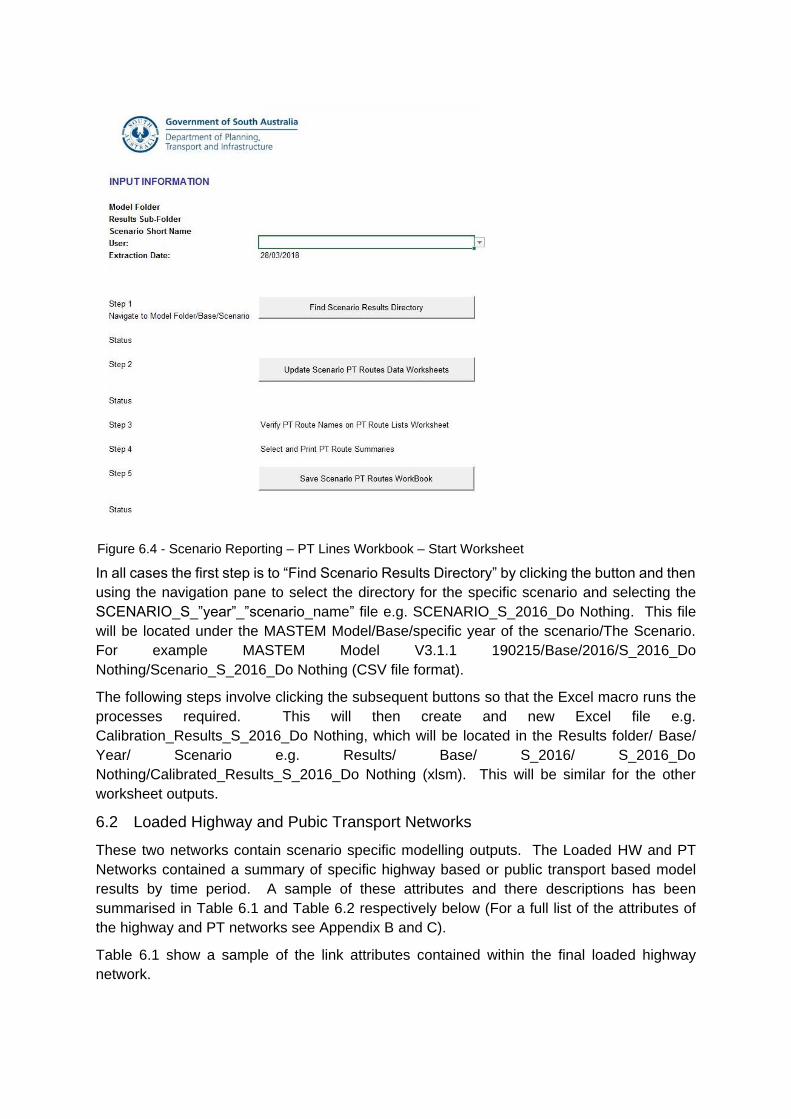
In all cases the first step is to “Find Scenario Results Directory” by clicking the button and then
using the navigation pane to select the directory for the specific scenario and selecting the
SCENARIO_S_”year”_”scenario_name” file e.g. SCENARIO_S_2016_Do Nothing. This file
will be located under the MASTEM Model/Base/specific year of the scenario/The Scenario.
For example MASTEM Model V3.1.1 190215/Base/2016/S_2016_Do
Nothing/Scenario_S_2016_Do Nothing (CSV file format).
The following steps involve clicking the subsequent buttons so that the Excel macro runs the
processes required. This will then create and new Excel file e.g.
Calibration_Results_S_2016_Do Nothing, which will be located in the Results folder/ Base/
Year/ Scenario e.g. Results/ Base/ S_2016/ S_2016_Do
Nothing/Calibrated_Results_S_2016_Do Nothing (xlsm). This will be similar for the other
worksheet outputs.
6.2 Loaded Highway and Pubic Transport Networks
These two networks contain scenario specific modelling outputs. The Loaded HW and PT
Networks contained a summary of specific highway based or public transport based model
results by time period. A sample of these attributes and there descriptions has been
summarised in Table 6.1 and Table 6.2 respectively below (For a full list of the attributes of
the highway and PT networks see Appendix B and C).
Table 6.1 show a sample of the link attributes contained within the final loaded highway
network.
Figure 6.4 - Scenario Reporting – PT Lines Workbook – Start Worksheet
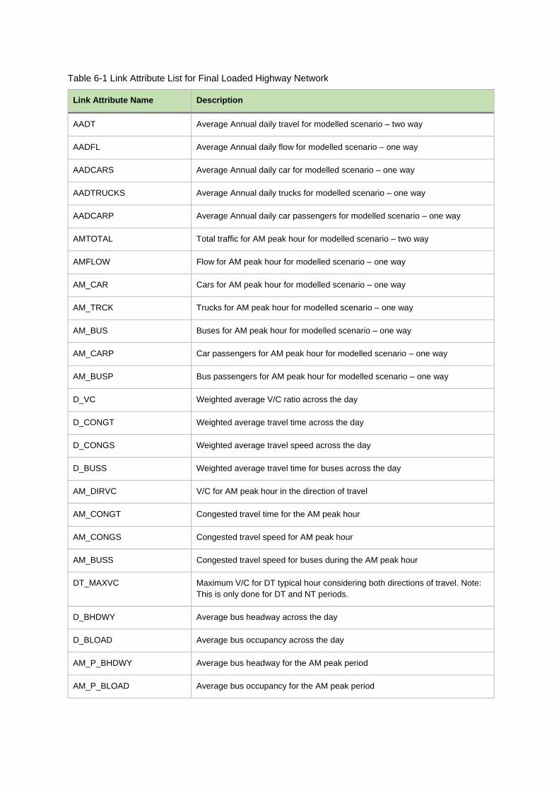
Link Attribute Name Description
AADT Average Annual daily travel for modelled scenario – two way
AADFL Average Annual daily flow for modelled scenario – one way
AADCARS Average Annual daily car for modelled scenario – one way
AADTRUCKS Average Annual daily trucks for modelled scenario – one way
AADCARP Average Annual daily car passengers for modelled scenario – one way
AMTOTAL Total traffic for AM peak hour for modelled scenario – two way
AMFLOW Flow for AM peak hour for modelled scenario – one way
AM_CAR Cars for AM peak hour for modelled scenario – one way
AM_TRCK Trucks for AM peak hour for modelled scenario – one way
AM_BUS Buses for AM peak hour for modelled scenario – one way
AM_CARP Car passengers for AM peak hour for modelled scenario – one way
AM_BUSP Bus passengers for AM peak hour for modelled scenario – one way
D_VC Weighted average V/C ratio across the day
D_CONGT Weighted average travel time across the day
D_CONGS Weighted average travel speed across the day
D_BUSS Weighted average travel time for buses across the day
AM_DIRVC V/C for AM peak hour in the direction of travel
AM_CONGT Congested travel time for the AM peak hour
AM_CONGS Congested travel speed for AM peak hour
AM_BUSS Congested travel speed for buses during the AM peak hour
DT_MAXVC Maximum V/C for DT typical hour considering both directions of travel. Note:
This is only done for DT and NT periods.
D_BHDWY Average bus headway across the day
D_BLOAD Average bus occupancy across the day
AM_P_BHDWY Average bus headway for the AM peak period
AM_P_BLOAD Average bus occupancy for the AM peak period
Table 6-1 Link Attribute List for Final Loaded Highway Network

Table 6.2 show a sample of the link attributes contained within the final loaded public transport
network.
Link Attribute Name Description
AMBUSES Number of buses for the AM peak period
AMBHDWY Average bus headway for the AM peak period
AMBPASS Number of bus passengers for the MA peak period
AMBLOAD Average bus occupancy for the AM peak period
AMBSPD_1 Average speed for mode 1 buses during the AM peak period (see Appendix
C1 for bus types)
AMBSPD_4 Average speed for mode 4 buses during the AM peak period (see Appendix
C1 for bus types)
AMBSPD_5 Average speed for mode 5 buses during the AM peak period (see Appendix
C1 for bus types)
AMBUS_SCAP Total AM period bus seated capacity for the link
AMBUS_CCAP Total AM period bus crush capacity for the link
AMTRAINS Number of trains for the AM peak period
AMTRNHDWY Average trains headway for the AM peak period
AMTRNPASS Number of train passengers for the MA peak period
AMTRNLOAD Average train occupancy for the AM peak period
AMTRNSPD Average train speed during the AM peak period
AMTRN_SCAP Total AM period train seated capacity for the link
AMTRN_CCAP Total AM period train crush capacity for the link
AMTRAMS Number of trams for the AM peak period
AMTRMHDWY Average trams headway for the AM peak period
AMTRMPASS Number of tram passengers for the MA peak period
AMTRMLOAD Average tram occupancy for the AM peak period
AMTRMSPD Average tram speed during the AM peak period
AMTRM_SCAP Total AM period tram seated capacity for the link
AMTRM_CCAP Total AM period tram crush capacity for the link
Table 6-2 Link Attributes List for Final Loaded Public Transport Network
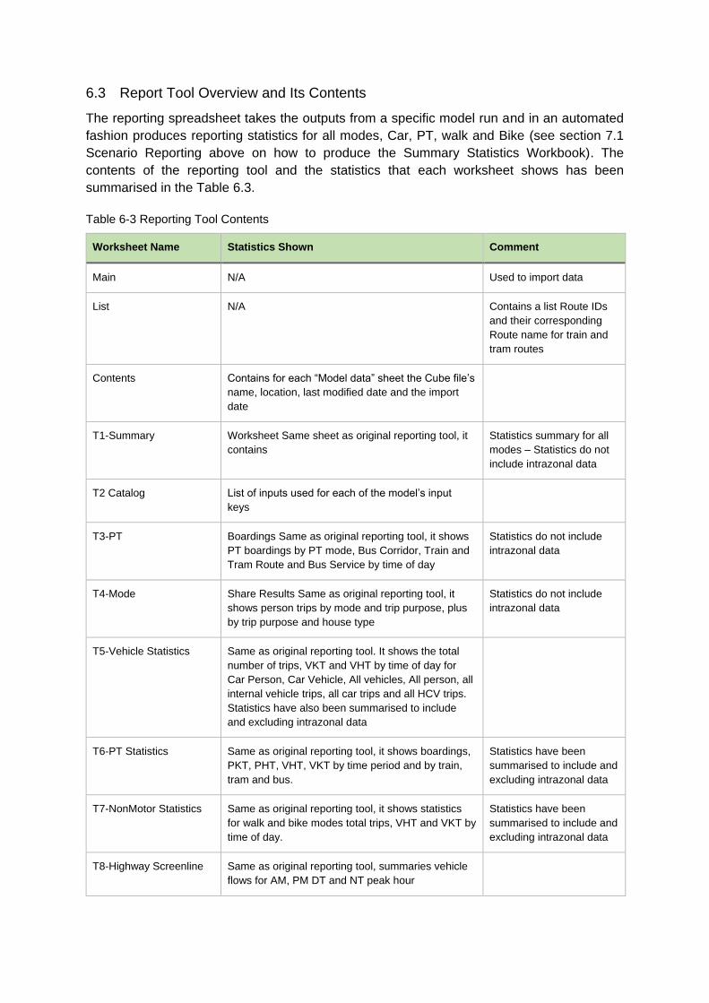
6.3 Report Tool Overview and Its Contents
The reporting spreadsheet takes the outputs from a specific model run and in an automated
fashion produces reporting statistics for all modes, Car, PT, walk and Bike (see section 7.1
Scenario Reporting above on how to produce the Summary Statistics Workbook). The
contents of the reporting tool and the statistics that each worksheet shows has been
summarised in the Table 6.3.
Worksheet Name Statistics Shown Comment
Main N/A Used to import data
List N/A Contains a list Route IDs
and their corresponding
Route name for train and
tram routes
Contents Contains for each “Model data” sheet the Cube file’s
name, location, last modified date and the import
date
T1-Summary Worksheet Same sheet as original reporting tool, it
contains
Statistics summary for all
modes – Statistics do not
include intrazonal data
T2 Catalog List of inputs used for each of the model’s input
keys
T3-PT Boardings Same as original reporting tool, it shows
PT boardings by PT mode, Bus Corridor, Train and
Tram Route and Bus Service by time of day
Statistics do not include
intrazonal data
T4-Mode Share Results Same as original reporting tool, it
shows person trips by mode and trip purpose, plus
by trip purpose and house type
Statistics do not include
intrazonal data
T5-Vehicle Statistics Same as original reporting tool. It shows the total
number of trips, VKT and VHT by time of day for
Car Person, Car Vehicle, All vehicles, All person, all
internal vehicle trips, all car trips and all HCV trips.
Statistics have also been summarised to include
and excluding intrazonal data
T6-PT Statistics Same as original reporting tool, it shows boardings,
PKT, PHT, VHT, VKT by time period and by train,
tram and bus.
Statistics have been
summarised to include and
excluding intrazonal data
T7-NonMotor Statistics Same as original reporting tool, it shows statistics
for walk and bike modes total trips, VHT and VKT by
time of day.
Statistics have been
summarised to include and
excluding intrazonal data
T8-Highway Screenline Same as original reporting tool, summaries vehicle
flows for AM, PM DT and NT peak hour
Table 6-3 Reporting Tool Contents
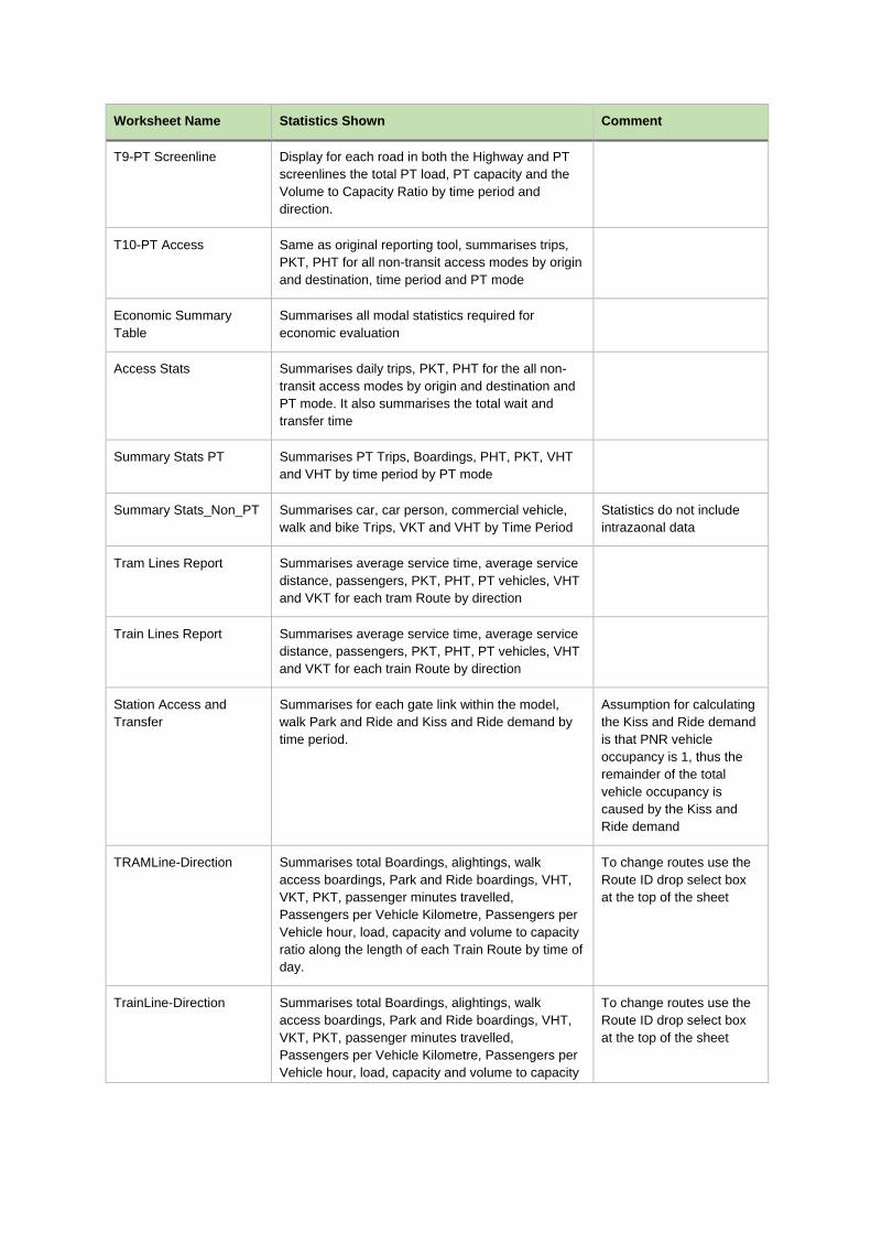
Worksheet Name Statistics Shown Comment
T9-PT Screenline Display for each road in both the Highway and PT
screenlines the total PT load, PT capacity and the
Volume to Capacity Ratio by time period and
direction.
T10-PT Access Same as original reporting tool, summarises trips,
PKT, PHT for all non-transit access modes by origin
and destination, time period and PT mode
Economic Summary
Table
Summarises all modal statistics required for
economic evaluation
Access Stats Summarises daily trips, PKT, PHT for the all non-
transit access modes by origin and destination and
PT mode. It also summarises the total wait and
transfer time
Summary Stats PT Summarises PT Trips, Boardings, PHT, PKT, VHT
and VHT by time period by PT mode
Summary Stats_Non_PT Summarises car, car person, commercial vehicle,
walk and bike Trips, VKT and VHT by Time Period
Statistics do not include
intrazaonal data
Tram Lines Report Summarises average service time, average service
distance, passengers, PKT, PHT, PT vehicles, VHT
and VKT for each tram Route by direction
Train Lines Report Summarises average service time, average service
distance, passengers, PKT, PHT, PT vehicles, VHT
and VKT for each train Route by direction
Station Access and
Transfer
Summarises for each gate link within the model,
walk Park and Ride and Kiss and Ride demand by
time period.
Assumption for calculating
the Kiss and Ride demand
is that PNR vehicle
occupancy is 1, thus the
remainder of the total
vehicle occupancy is
caused by the Kiss and
Ride demand
TRAMLine-Direction Summarises total Boardings, alightings, walk
access boardings, Park and Ride boardings, VHT,
VKT, PKT, passenger minutes travelled,
Passengers per Vehicle Kilometre, Passengers per
Vehicle hour, load, capacity and volume to capacity
ratio along the length of each Train Route by time of
day.
To change routes use the
Route ID drop select box
at the top of the sheet
TrainLine-Direction Summarises total Boardings, alightings, walk
access boardings, Park and Ride boardings, VHT,
VKT, PKT, passenger minutes travelled,
Passengers per Vehicle Kilometre, Passengers per
Vehicle hour, load, capacity and volume to capacity
To change routes use the
Route ID drop select box
at the top of the sheet
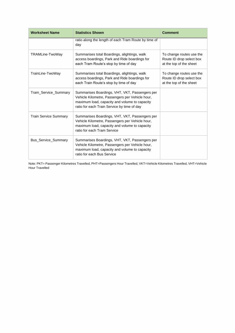
Worksheet Name Statistics Shown Comment
ratio along the length of each Tram Route by time of
day
TRAMLine-TwoWay Summarises total Boardings, alightings, walk
access boardings, Park and Ride boardings for
each Tram Route’s stop by time of day
To change routes use the
Route ID drop select box
at the top of the sheet
TrainLine-TwoWay Summarises total Boardings, alightings, walk
access boardings, Park and Ride boardings for
each Train Route’s stop by time of day
To change routes use the
Route ID drop select box
at the top of the sheet
Tram_Service_Summary Summarises Boardings, VHT, VKT, Passengers per
Vehicle Kilometre, Passengers per Vehicle hour,
maximum load, capacity and volume to capacity
ratio for each Train Service by time of day
Train Service Summary Summarises Boardings, VHT, VKT, Passengers per
Vehicle Kilometre, Passengers per Vehicle hour,
maximum load, capacity and volume to capacity
ratio for each Tram Service
Bus_Service_Summary Summarises Boardings, VHT, VKT, Passengers per
Vehicle Kilometre, Passengers per Vehicle hour,
maximum load, capacity and volume to capacity
ratio for each Bus Service
Note: PKT= Passenger Kilometres Travelled, PHT=Passengers Hour Travelled, VKT=Vehicle Kilometres Travelled, VHT=Vehicle
Hour Travelled
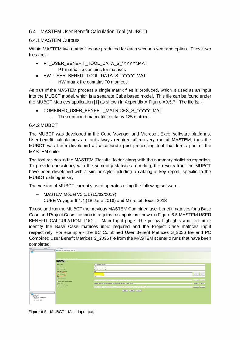
6.4 MASTEM User Benefit Calculation Tool (MUBCT)
6.4.1 MASTEM Outputs
Within MASTEM two matrix files are produced for each scenario year and option. These two
files are: -
PT_USER_BENEFIT_TOOL_DATA_S_”YYYY”.MAT
PT matrix file contains 55 matrices
HW_USER_BENFIT_TOOL_DATA_S_”YYYY”.MAT
HW matrix file contains 70 matrices
As part of the MASTEM process a single matrix files is produced, which is used as an input
into the MUBCT model, which is a separate Cube based model. This file can be found under
the MUBCT Matrices application [1] as shown in Appendix A Figure A9.5.7. The file is: -
COMBINED_USER_BENEFIT_MATRICES_S_”YYYY”.MAT
The combined matrix file contains 125 matrices
6.4.2 MUBCT
The MUBCT was developed in the Cube Voyager and Microsoft Excel software platforms.
User-benefit calculations are not always required after every run of MASTEM, thus the
MUBCT was been developed as a separate post-processing tool that forms part of the
MASTEM suite.
The tool resides in the MASTEM ‘Results’ folder along with the summary statistics reporting.
To provide consistency with the summary statistics reporting, the results from the MUBCT
have been developed with a similar style including a catalogue key report, specific to the
MUBCT catalogue key.
The version of MUBCT currently used operates using the following software:
MASTEM Model V3.1.1 (15/02/2019)
CUBE Voyager 6.4.4 (18 June 2018) and Microsoft Excel 2013
To use and run the MUBCT the previous MASTEM Combined user benefit matrices for a Base
Case and Project Case scenario is required as inputs as shown in Figure 6.5 MASTEM USER
BENEFIT CALCULATION TOOL – Main Input page. The yellow highlights and red circle
identify the Base Case matrices input required and the Project Case matrices input
respectively. For example - the BC Combined User Benefit Matrices S_2036 file and PC
Combined User Benefit Matrices S_2036 file from the MASTEM scenario runs that have been
completed.
Figure 6.5 - MUBCT - Main input page
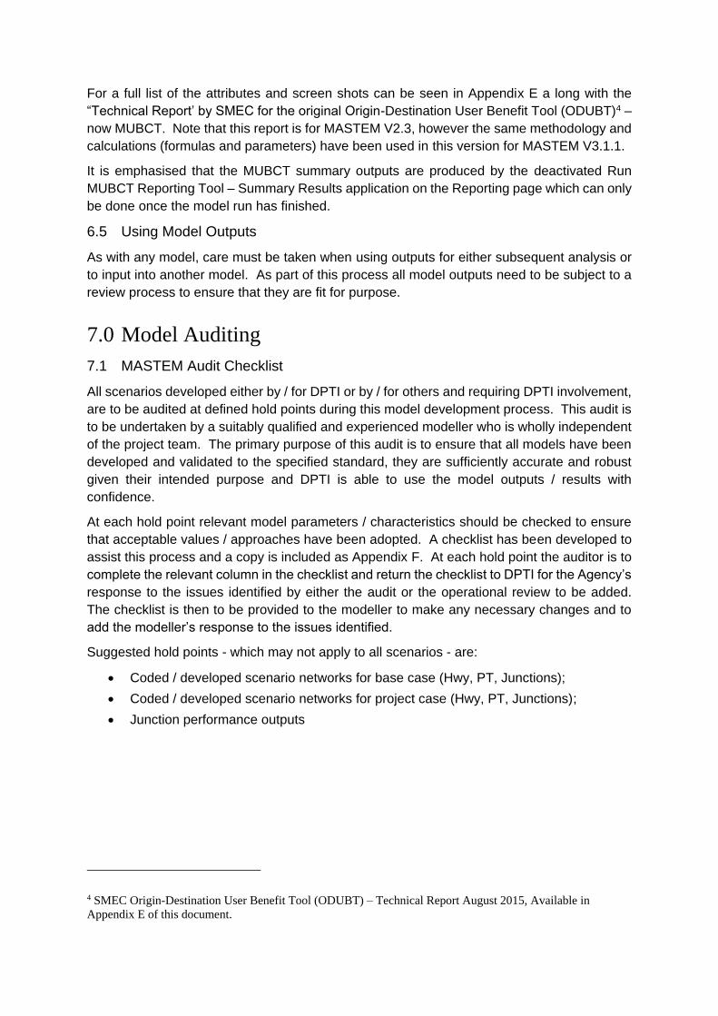
For a full list of the attributes and screen shots can be seen in Appendix E a long with the
“Technical Report’ by SMEC for the original Origin-Destination User Benefit Tool (ODUBT)4 –
now MUBCT. Note that this report is for MASTEM V2.3, however the same methodology and
calculations (formulas and parameters) have been used in this version for MASTEM V3.1.1.
It is emphasised that the MUBCT summary outputs are produced by the deactivated Run
MUBCT Reporting Tool – Summary Results application on the Reporting page which can only
be done once the model run has finished.
6.5 Using Model Outputs
As with any model, care must be taken when using outputs for either subsequent analysis or
to input into another model. As part of this process all model outputs need to be subject to a
review process to ensure that they are fit for purpose.
7.0 Model Auditing
7.1 MASTEM Audit Checklist
All scenarios developed either by / for DPTI or by / for others and requiring DPTI involvement,
are to be audited at defined hold points during this model development process. This audit is
to be undertaken by a suitably qualified and experienced modeller who is wholly independent
of the project team. The primary purpose of this audit is to ensure that all models have been
developed and validated to the specified standard, they are sufficiently accurate and robust
given their intended purpose and DPTI is able to use the model outputs / results with
confidence.
At each hold point relevant model parameters / characteristics should be checked to ensure
that acceptable values / approaches have been adopted. A checklist has been developed to
assist this process and a copy is included as Appendix F. At each hold point the auditor is to
complete the relevant column in the checklist and return the checklist to DPTI for the Agency’s
response to the issues identified by either the audit or the operational review to be added.
The checklist is then to be provided to the modeller to make any necessary changes and to
add the modeller’s response to the issues identified.
Suggested hold points - which may not apply to all scenarios - are:
Coded / developed scenario networks for base case (Hwy, PT, Junctions);
Coded / developed scenario networks for project case (Hwy, PT, Junctions);
Junction performance outputs
4 SMEC Origin-Destination User Benefit Tool (ODUBT) – Technical Report August 2015, Available in
Appendix E of this document.

Appendix A – MASTEM Model Structure
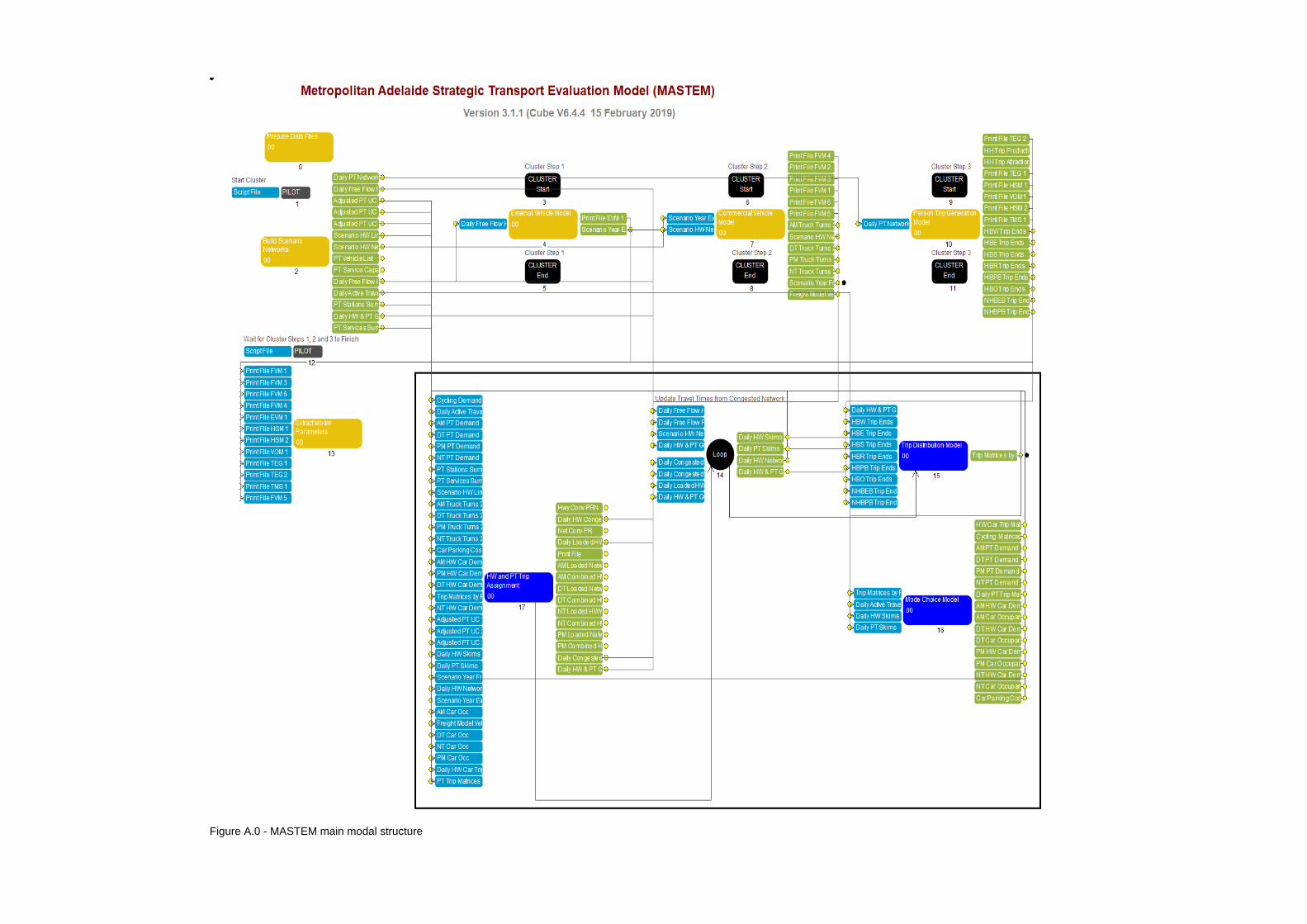
Figure A.0 - MASTEM main modal structure
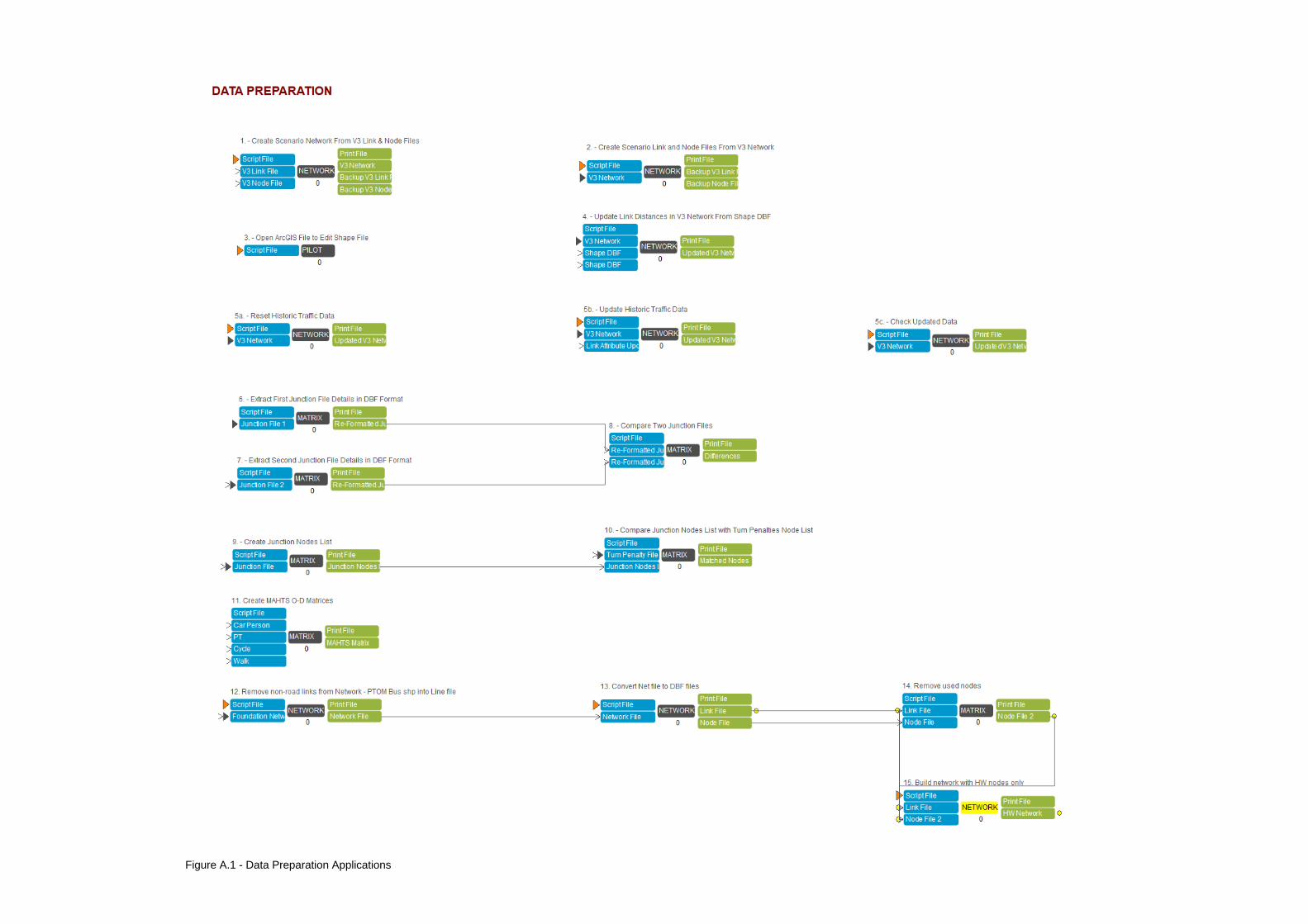
Figure A.1 - Data Preparation Applications
Figure A.2 - Build Scenario Networks Applications

Figure A.3 - External Vehicle Model Applications
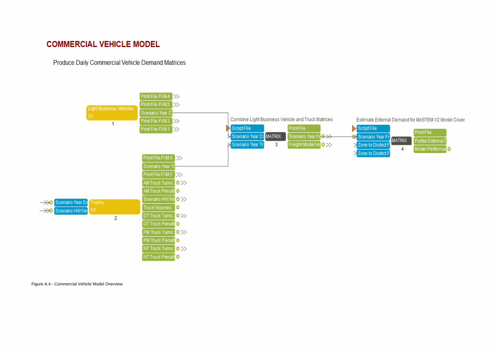
Figure A.4 - Commercial Vehicle Model Overview
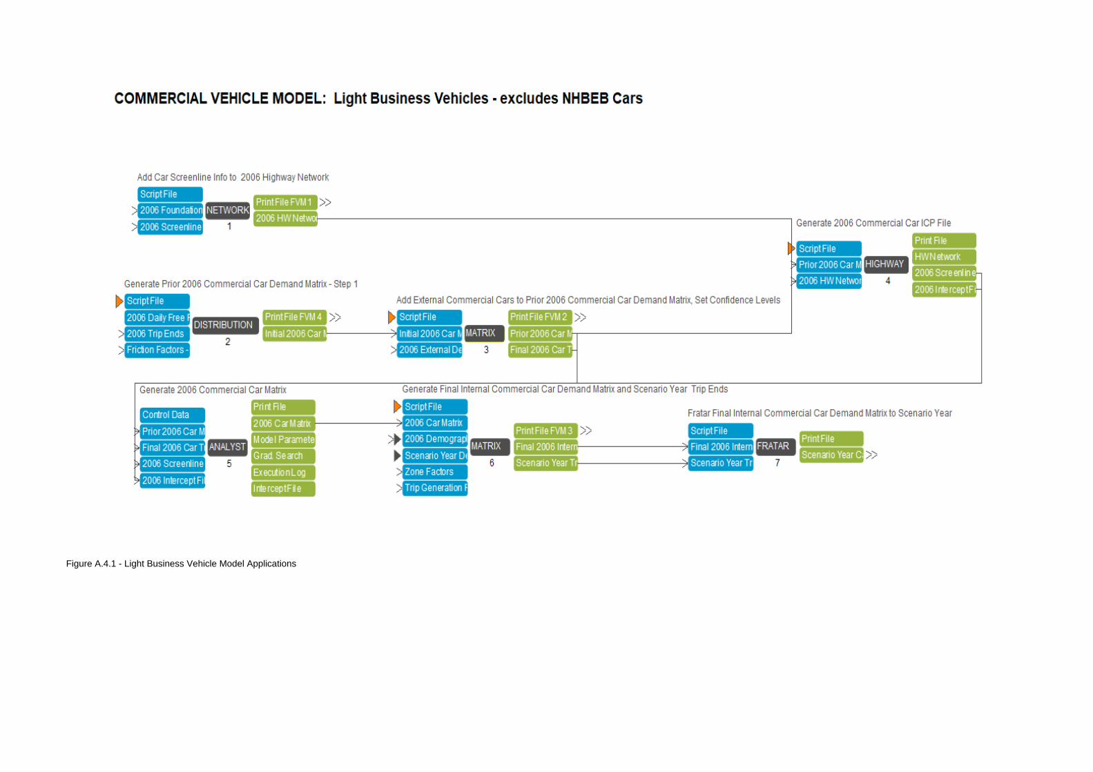
Figure A.4.1 - Light Business Vehicle Model Applications
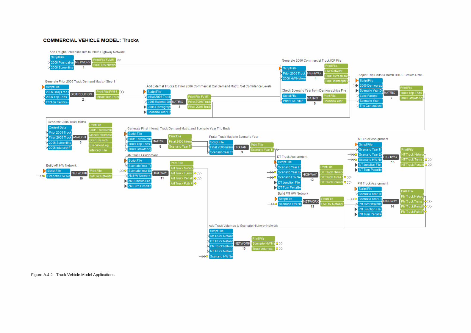
Figure A4.2 Truck Vehicle Model Applications Figure A.4.2 - Truck Vehicle Model Applications
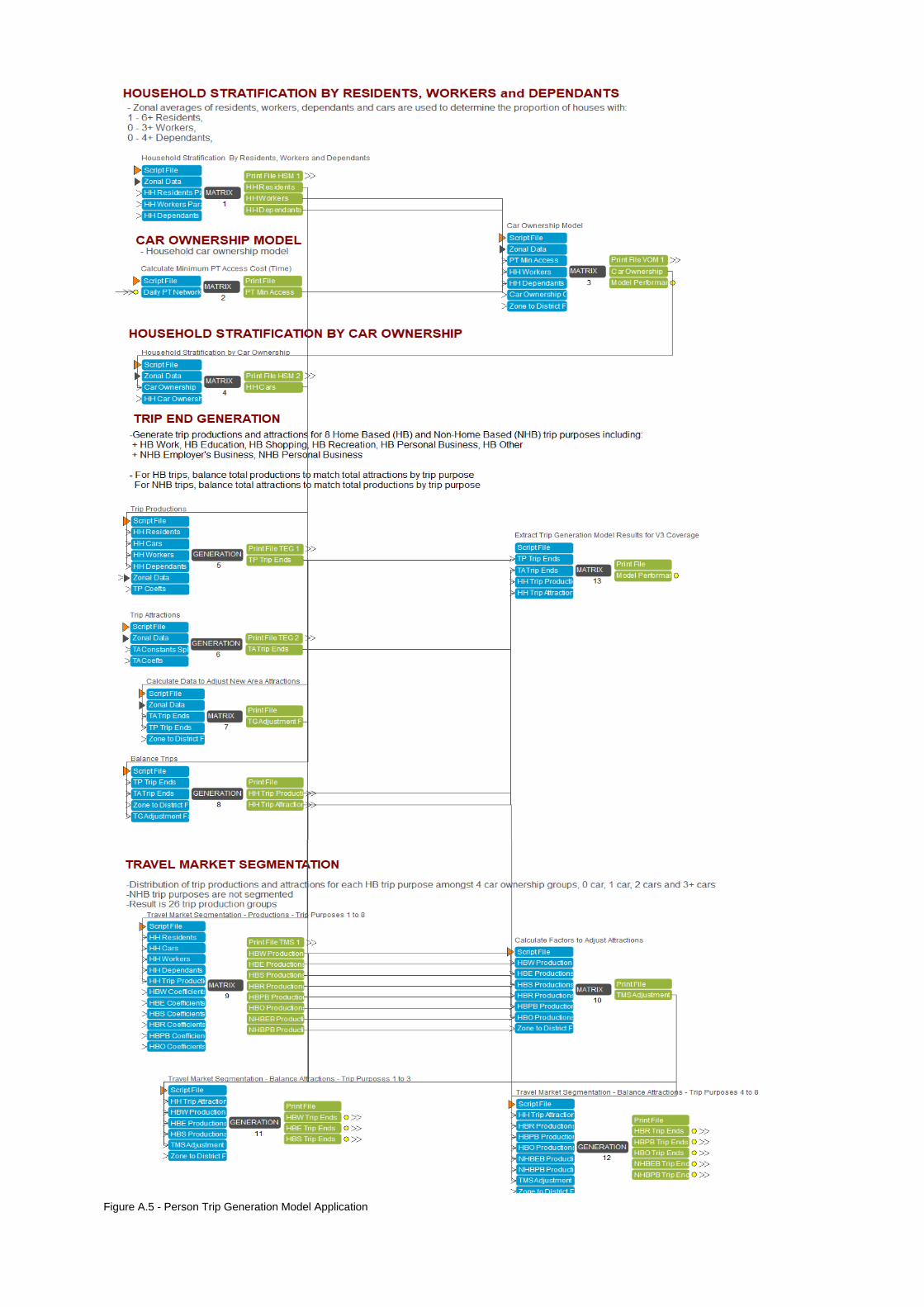
Figure A.5 - Person Trip Generation Model Application
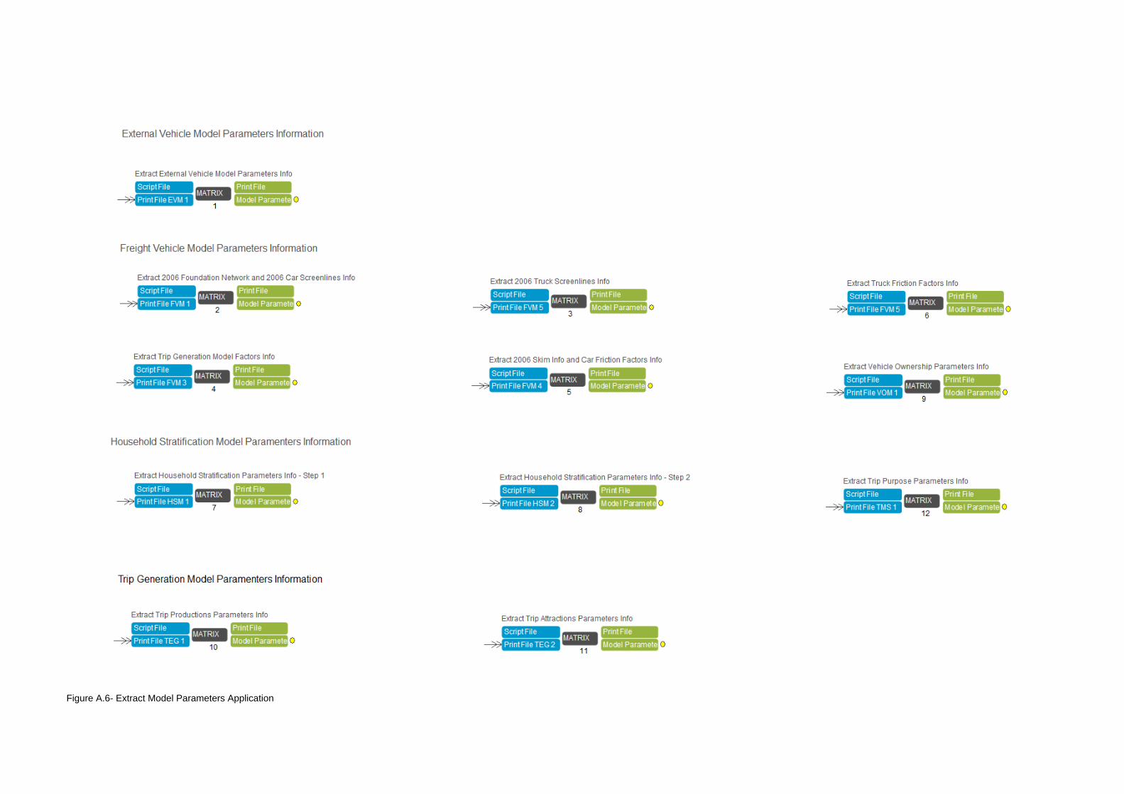
Figure A.6- Extract Model Parameters Application

Figure A.7 - Trip Distribution Model Application
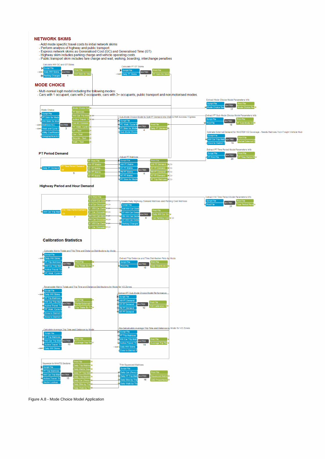
Figure A.8 - Mode Choice Model Application
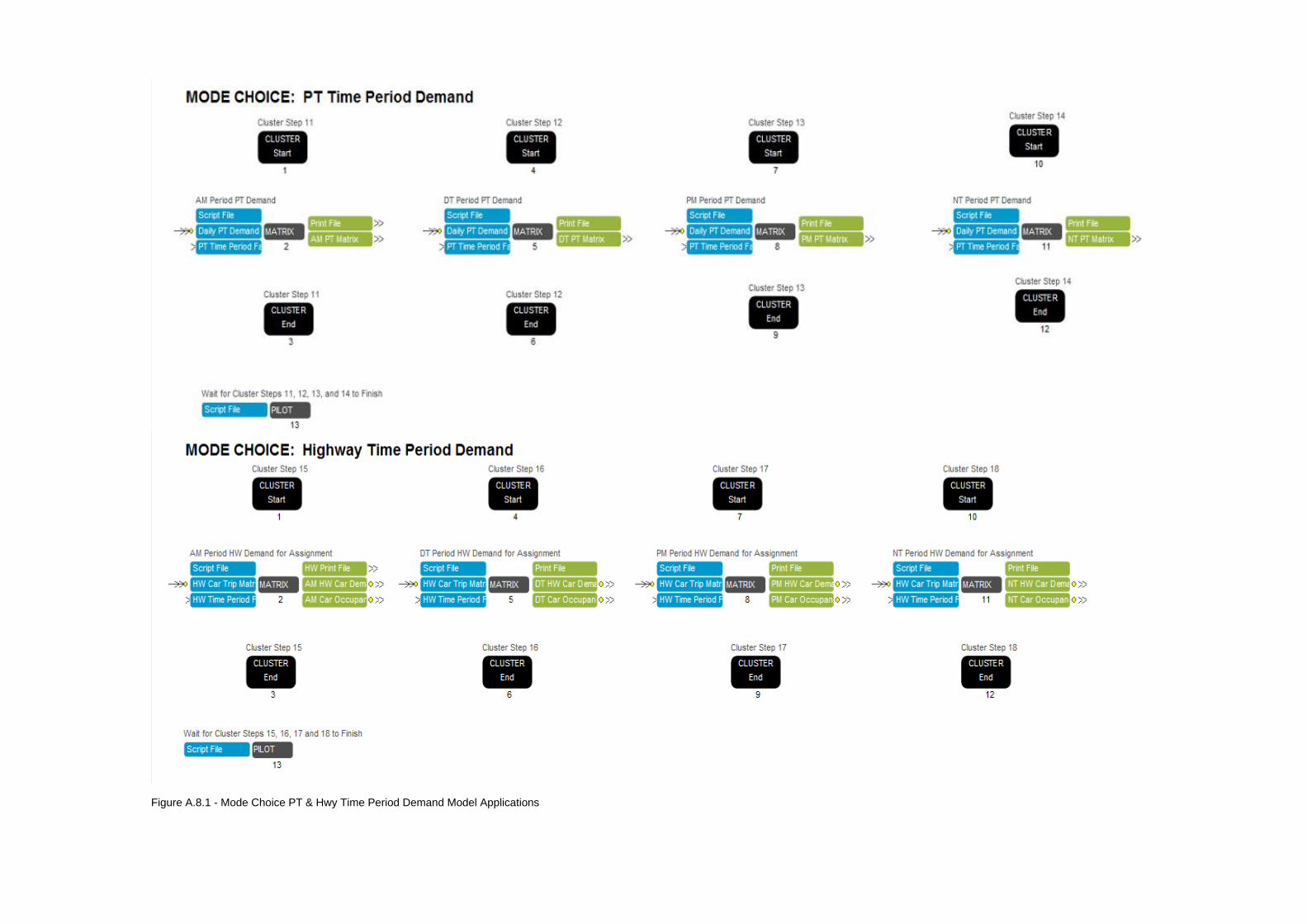
Figure A.8.1 - Mode Choice PT & Hwy Time Period Demand Model Applications

Figure A.9 - Highway and Public Transport Trip Assignment Model Applications
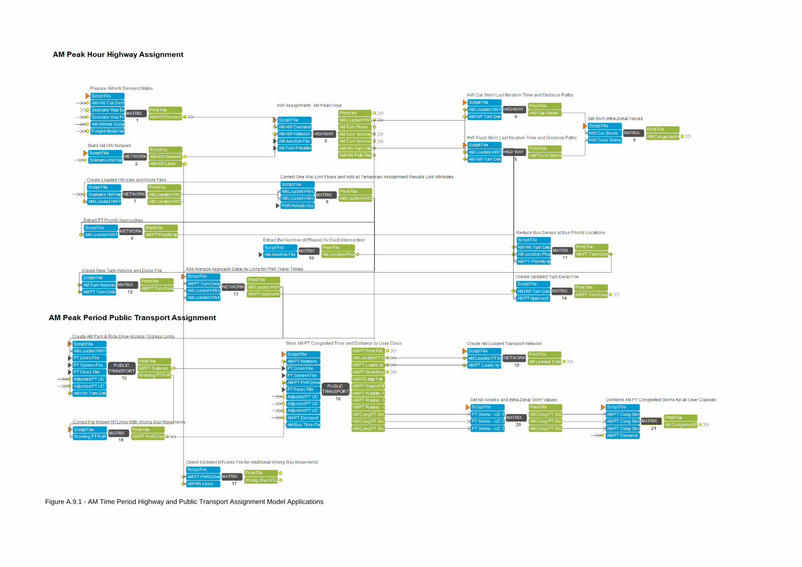
Figure A.9.1 - AM Time Period Highway and Public Transport Assignment Model Applications
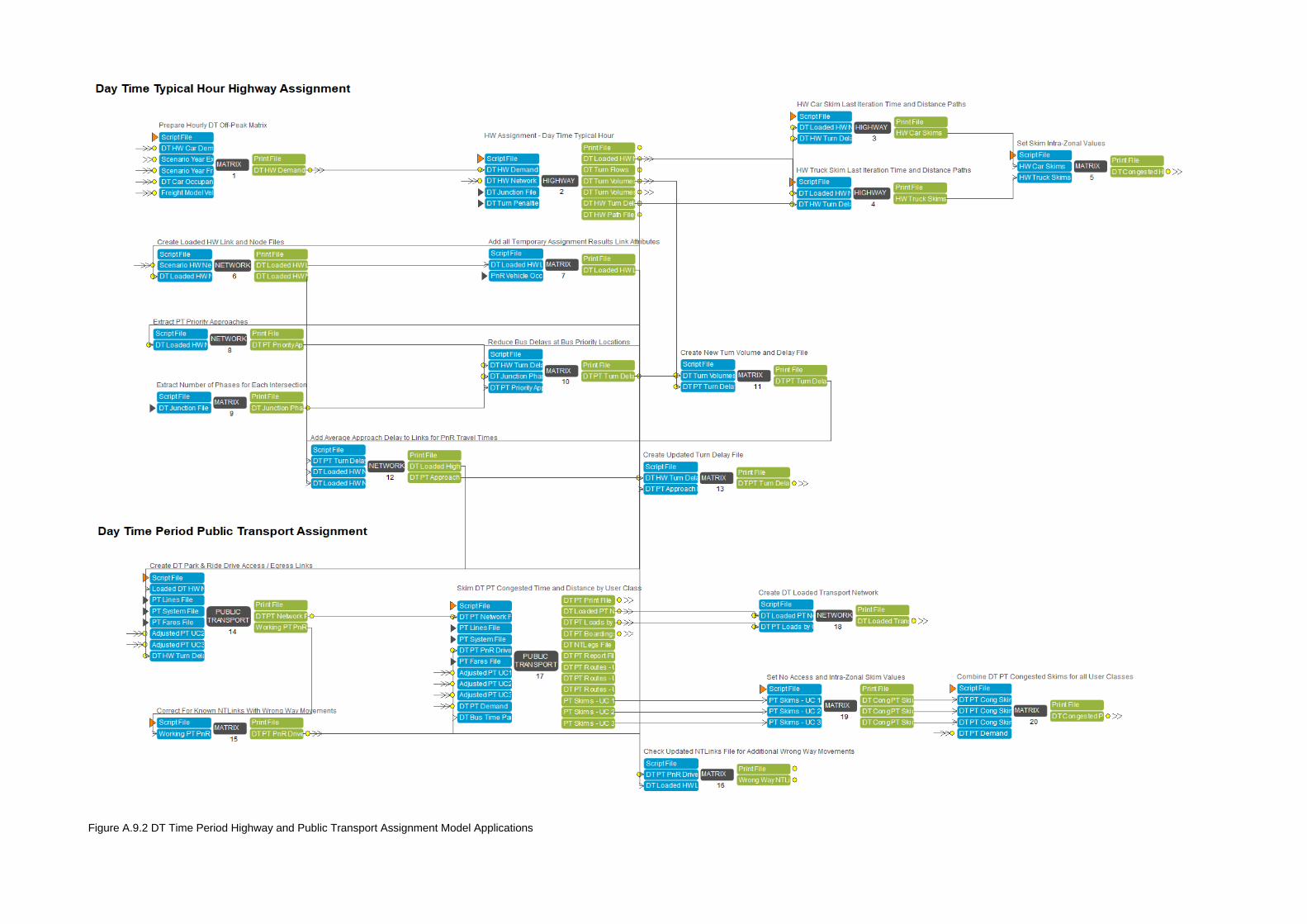
Figure 0.1 - DT Time Period Highway and Public Transport Assignment Model Applications Figure A.9.2 DT Time Period Highway and Public Transport Assignment Model Applications
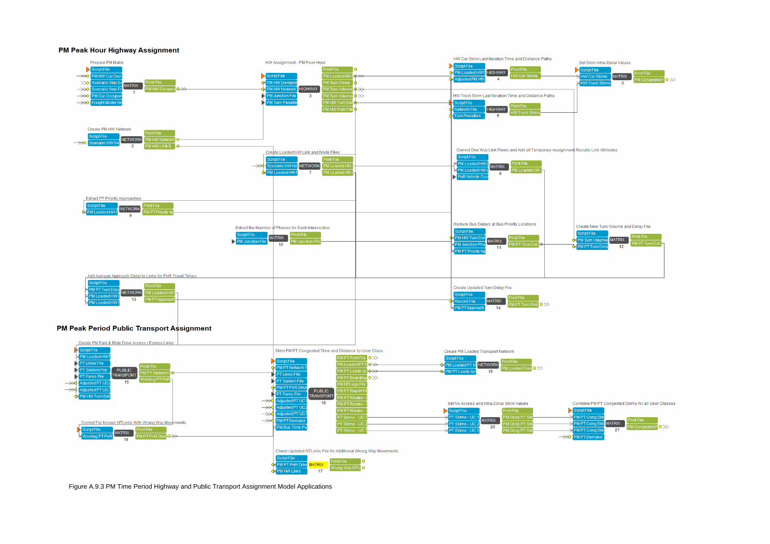
Figure A.9.3 PM Time Period Highway and Public Transport Assignment Model Applications
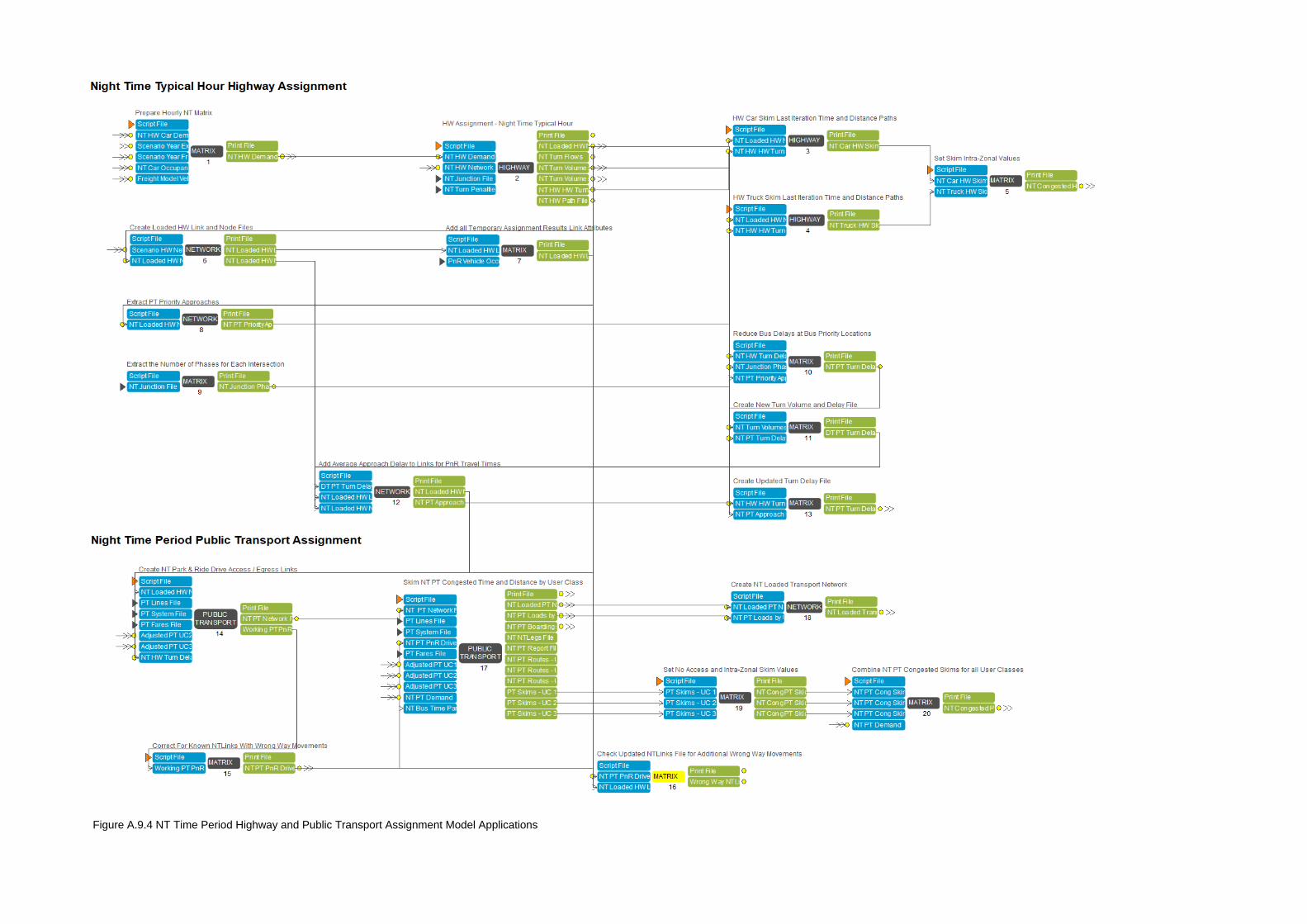
Figure A.9.4 NT Time Period Highway and Public Transport Assignment Model Applications
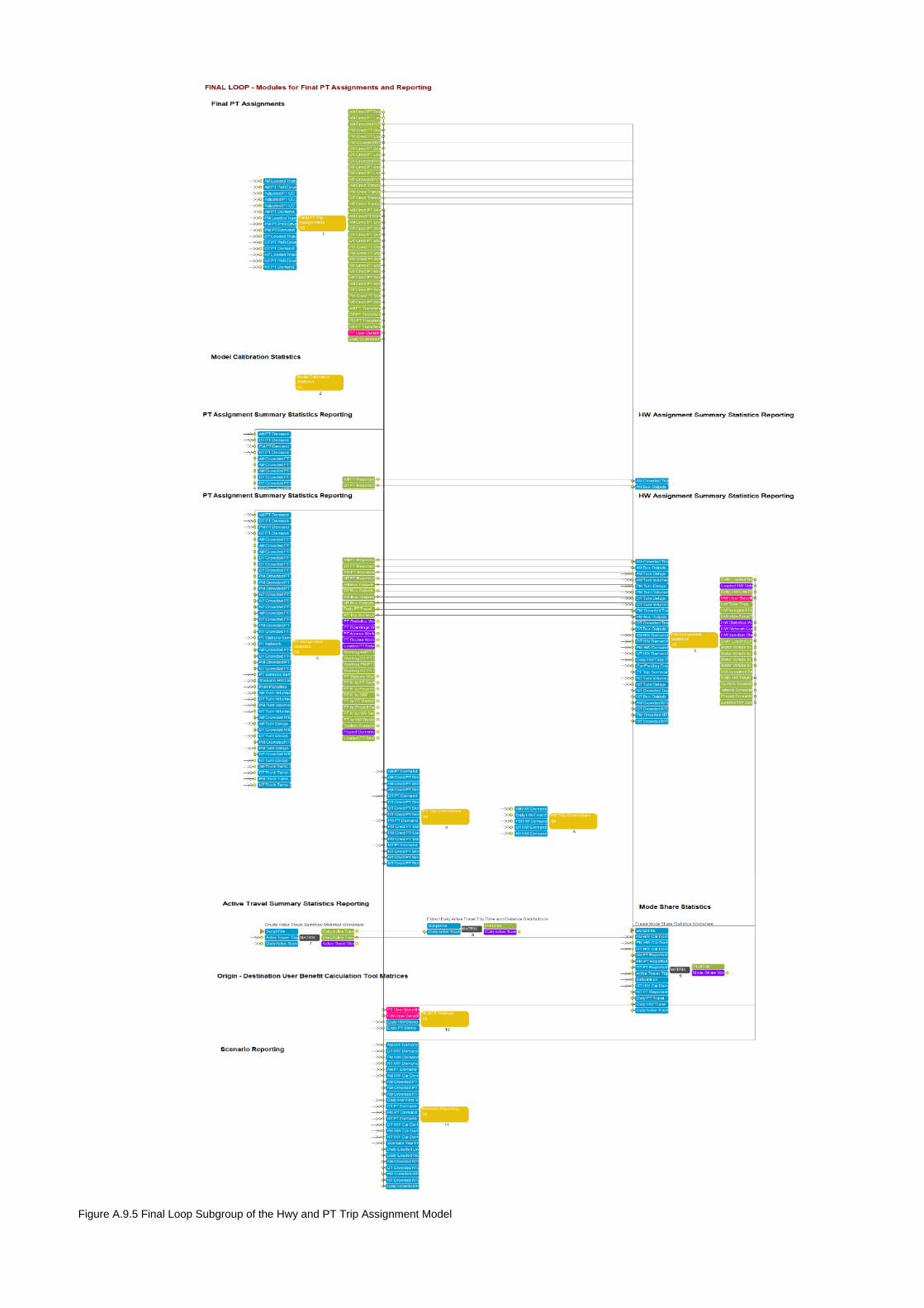
Figure A.9.5 Final Loop Subgroup of the Hwy and PT Trip Assignment Model
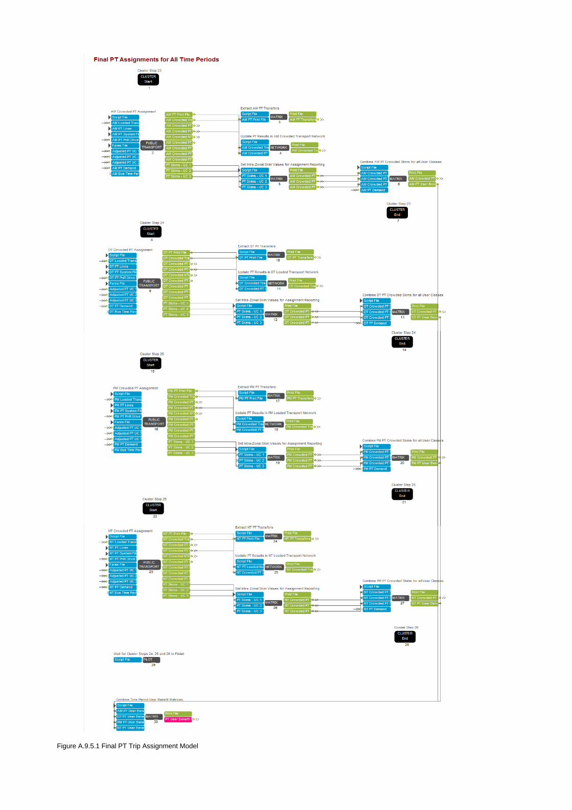
Figure A.9.5.1 Final PT Trip Assignment Model
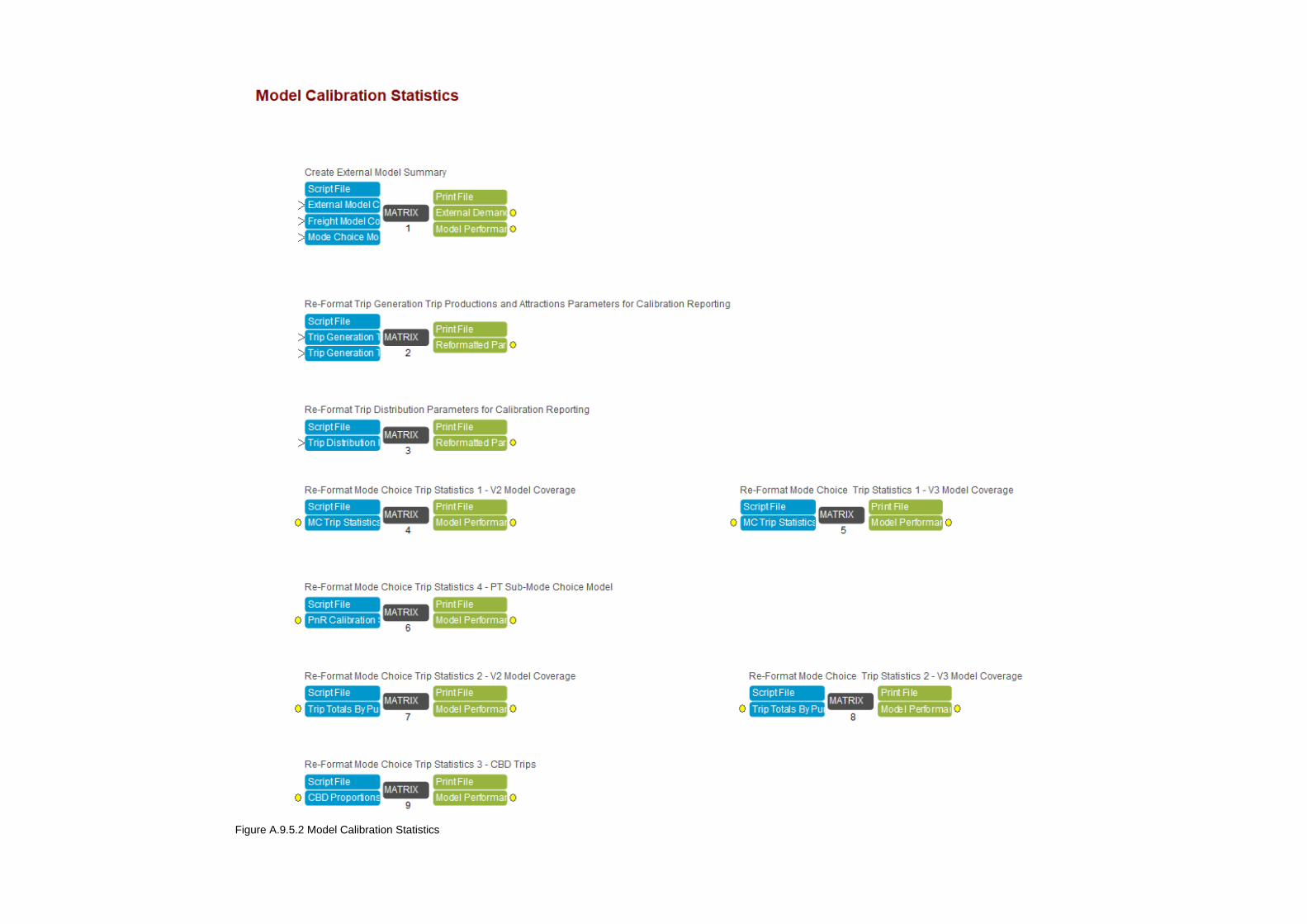
Figure A.9.5.2 Model Calibration Statistics
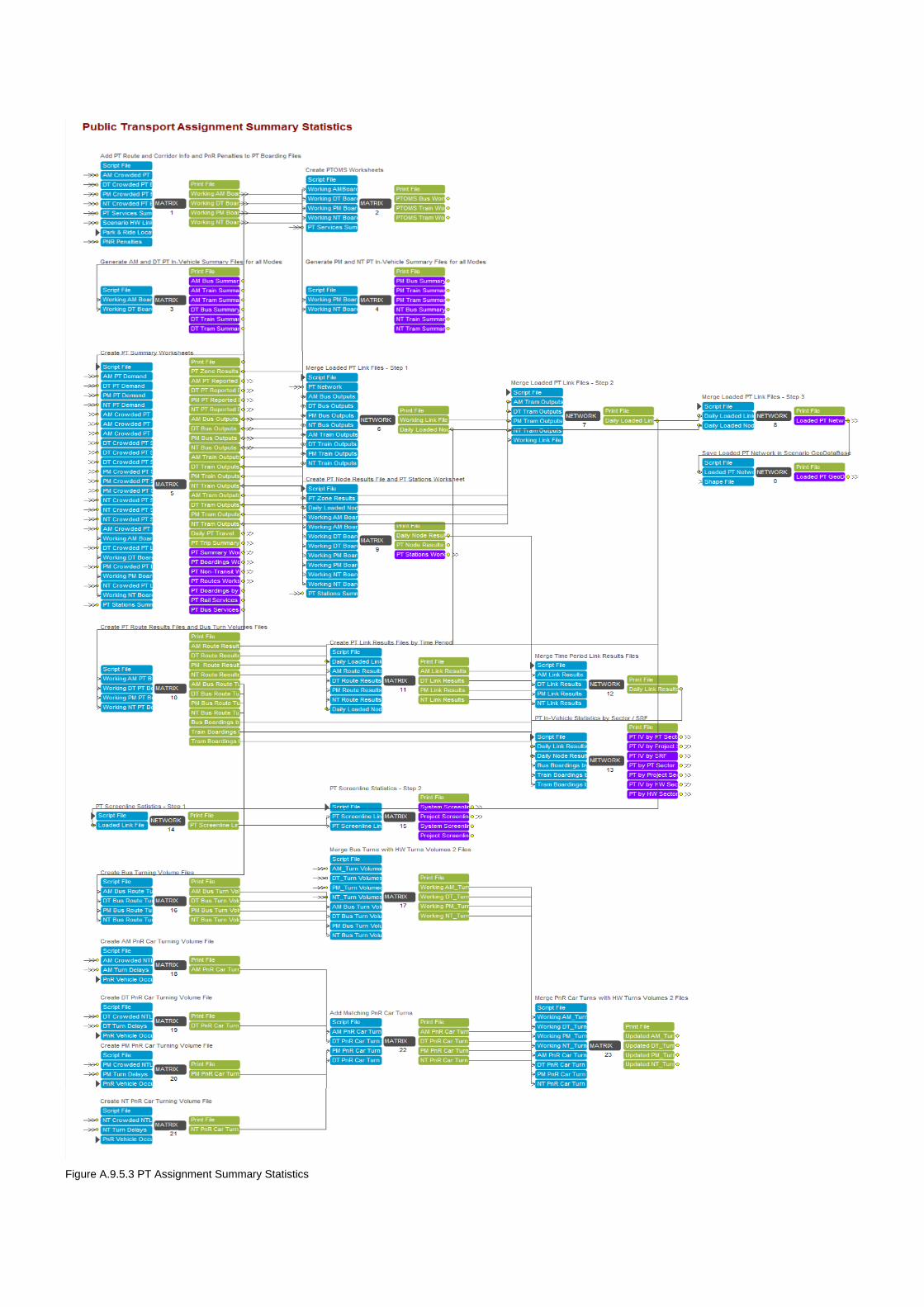
Figure A.9.5.3 PT Assignment Summary Statistics
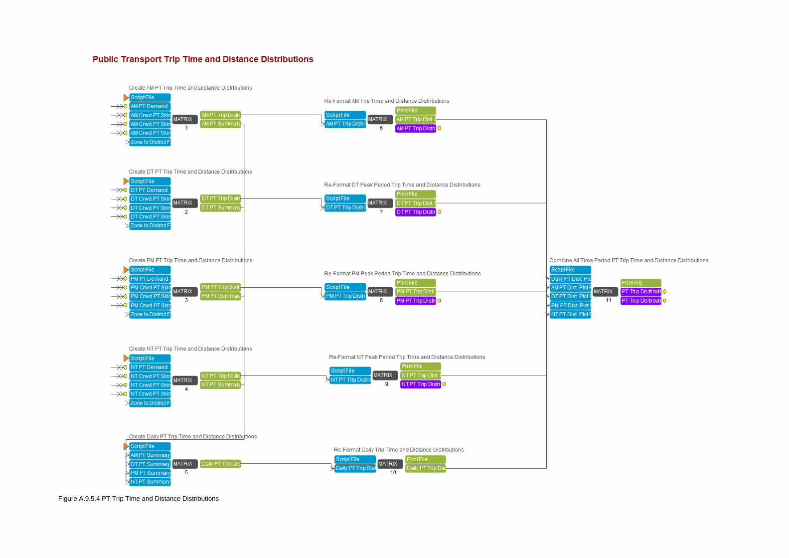
Figure A.9.5.4 PT Trip Time and Distance Distributions

Figure A.9.5.5 Highway Assignment Summary Statistics
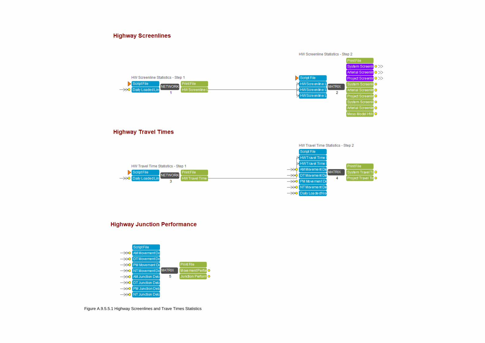
Figure A.9.5.5.1 Highway Screenlines and Trave Times Statistics
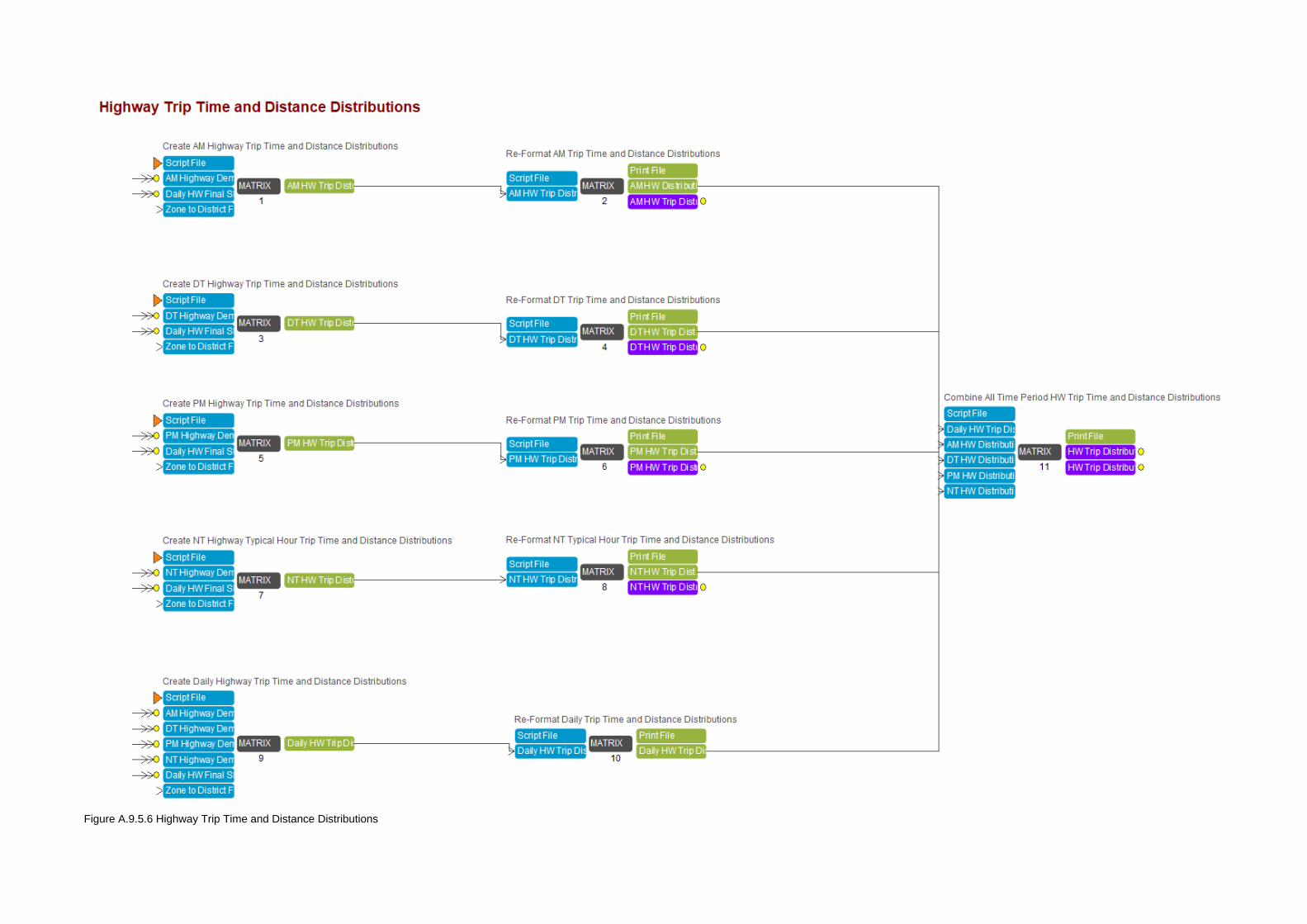
Figure A.9.5.6 Highway Trip Time and Distance Distributions
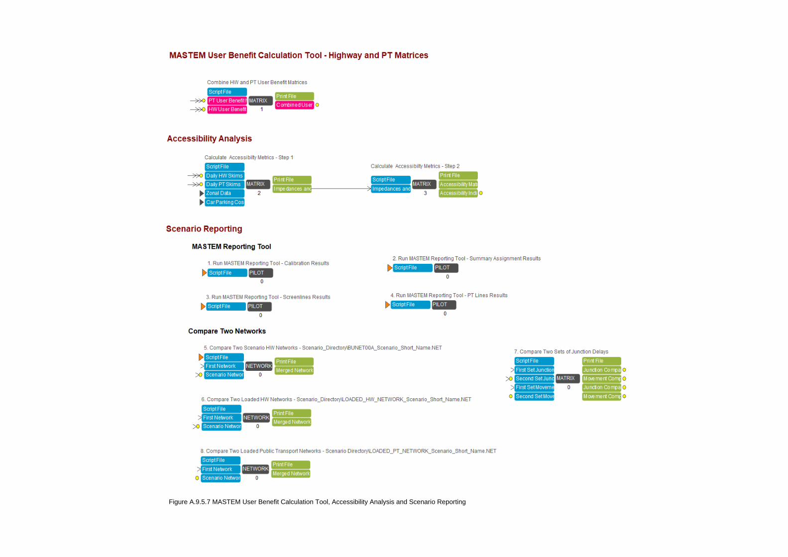
Figure A.9.5.7 MASTEM User Benefit Calculation Tool, Accessibility Analysis and Scenario Reporting

Appendix B – Foundation Network Updating
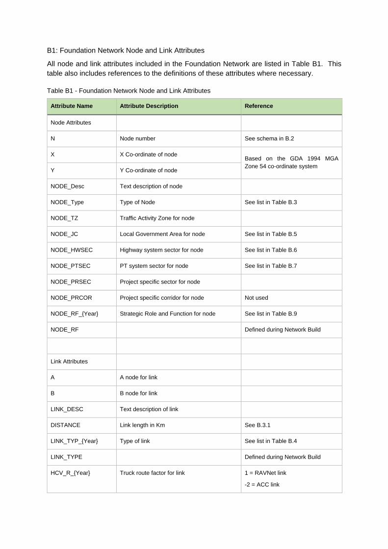
B1: Foundation Network Node and Link Attributes
All node and link attributes included in the Foundation Network are listed in Table B1. This
table also includes references to the definitions of these attributes where necessary.
Attribute Name Attribute Description Reference
Node Attributes
N Node number See schema in B.2
X X Co-ordinate of node Based on the GDA 1994 MGA
Zone 54 co-ordinate system Y Y Co-ordinate of node
NODE_Desc Text description of node
NODE_Type Type of Node See list in Table B.3
NODE_TZ Traffic Activity Zone for node
NODE_JC Local Government Area for node See list in Table B.5
NODE_HWSEC Highway system sector for node See list in Table B.6
NODE_PTSEC PT system sector for node See list in Table B.7
NODE_PRSEC Project specific sector for node
NODE_PRCOR Project specific corridor for node Not used
NODE_RF_{Year} Strategic Role and Function for node See list in Table B.9
NODE_RF Defined during Network Build
Link Attributes
A A node for link
B B node for link
LINK_DESC Text description of link
DISTANCE Link length in Km See B.3.1
LINK_TYP_{Year} Type of link See list in Table B.4
LINK_TYPE Defined during Network Build
HCV_R_{Year} Truck route factor for link 1 = RAVNet link
-2 = ACC link
Table B1 - Foundation Network Node and Link Attributes

Attribute Name Attribute Description Reference
0 = Otherwise
HCV_ROUTE Defined during Network Build
LINK_TZ Traffic Activity Zone for link
LINK_JC Local Government Area for link See list in Table B.5
LINK_HWSEC Highway system sector for link See list in Table B.6
LINK_PTSEC PT system sector for link See list in Table B.7
LINK_HWTT HW travel time route for link See definition in Table B.8
LINK_PRSEC Project specific sector for link
LINK_PRCOR Project specific corridor for link
LINK_PRSL Project specific screenline code for link
LINK_RF_{Year} Strategic Role and Function for link See list in Table B.9
LINK_RF Defined during Network Build
LINK_{Year} Determines if link is present in modelled year 1 = Present,
0 = Deleted
AM_LINK Determines if link is present in AM peak
period
1 = Present,
0 = Deleted
PM_LINK Determines if link is present in PM peak
period
1 = Present,
0 = Deleted
BUS_P_{Year} Determines if there is bus priority on this
approach to the link’s B-node
0 = N/A
1 = all day
2 = both peaks
2 = am only
4 = pm only
5 = both peaks and day time
BUS_PTY Defined during Network Build
BUS_L_{Year} Determines if there is bus lane on this link 0 = N/A
1 = all day
2 = both peaks
3 = am only
4 = pm only
5 = both peaks and day time
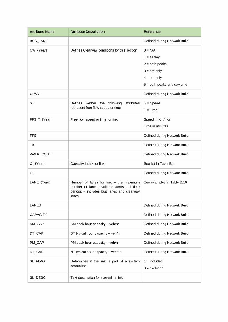
Attribute Name Attribute Description Reference
BUS_LANE Defined during Network Build
CW_{Year} Defines Clearway conditions for this section 0 = N/A
1 = all day
2 = both peaks
3 = am only
4 = pm only
5 = both peaks and day time
CLWY Defined during Network Build
ST Defines wether the following attributes
represent free flow speed or time
S = Speed
T = Time
FFS_T_[Year] Free flow speed or time for link Speed in Km/h or
Time in minutes
FFS Defined during Network Build
T0 Defined during Network Build
WALK_COST Defined during Network Build
CI_{Year} Capacity Index for link See list in Table B.4
CI Defined during Network Build
LANE_{Year} Number of lanes for link – the maximum
number of lanes available across all time
periods – includes bus lanes and clearway
lanes
See examples in Table B.10
LANES Defined during Network Build
CAPACITY Defined during Network Build
AM_CAP AM peak hour capacity – veh/hr Defined during Network Build
DT_CAP DT typical hour capacity – veh/hr Defined during Network Build
PM_CAP PM peak hour capacity – veh/hr Defined during Network Build
NT_CAP NT typical hour capacity – veh/hr Defined during Network Build
SL_FLAG Determines if the link is part of a system
screenline
1 = included
0 = excluded
SL_DESC Text description for screenline link
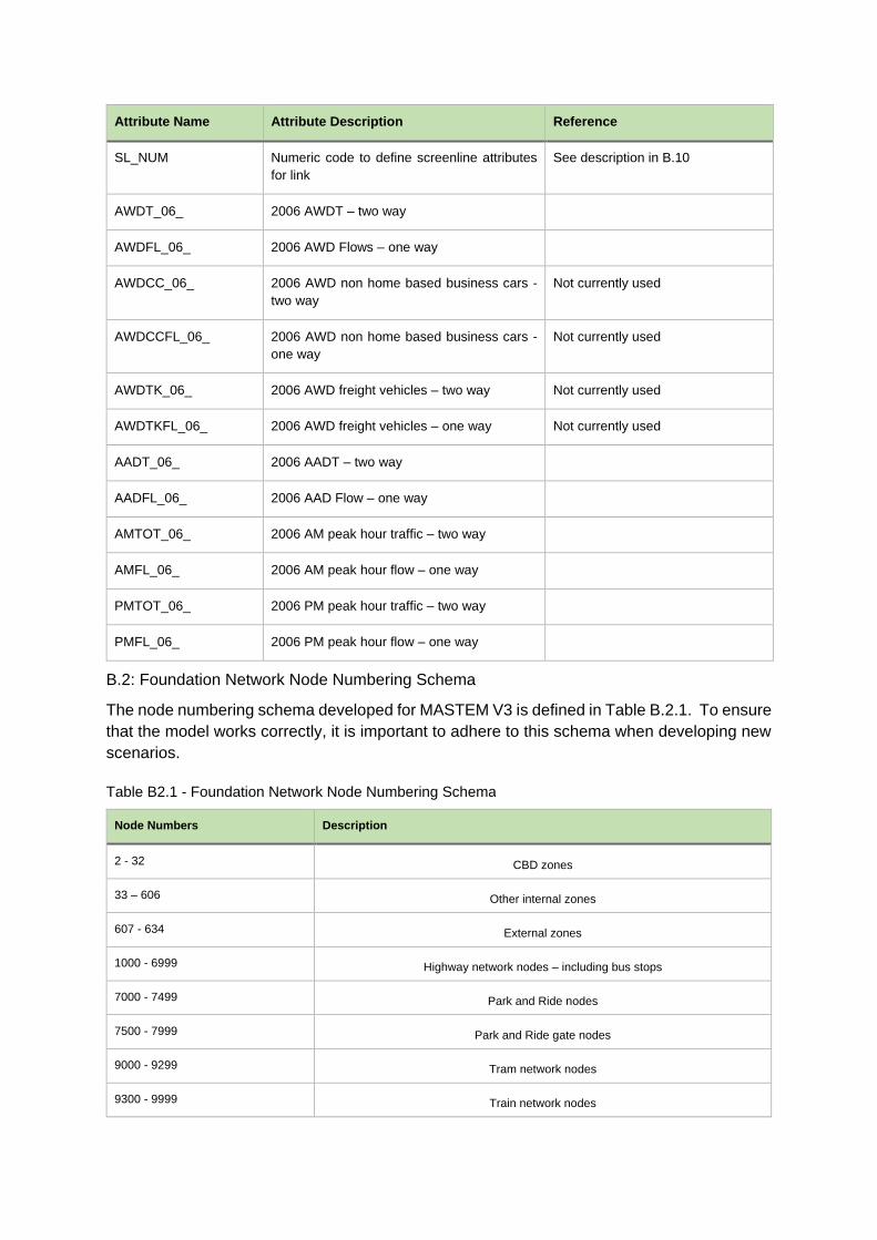
Attribute Name Attribute Description Reference
SL_NUM Numeric code to define screenline attributes
for link
See description in B.10
AWDT_06_ 2006 AWDT – two way
AWDFL_06_ 2006 AWD Flows – one way
AWDCC_06_ 2006 AWD non home based business cars -
two way
Not currently used
AWDCCFL_06_ 2006 AWD non home based business cars -
one way
Not currently used
AWDTK_06_ 2006 AWD freight vehicles – two way Not currently used
AWDTKFL_06_ 2006 AWD freight vehicles – one way Not currently used
AADT_06_ 2006 AADT – two way
AADFL_06_ 2006 AAD Flow – one way
AMTOT_06_ 2006 AM peak hour traffic – two way
AMFL_06_ 2006 AM peak hour flow – one way
PMTOT_06_ 2006 PM peak hour traffic – two way
PMFL_06_ 2006 PM peak hour flow – one way
B.2: Foundation Network Node Numbering Schema
The node numbering schema developed for MASTEM V3 is defined in Table B.2.1. To ensure
that the model works correctly, it is important to adhere to this schema when developing new
scenarios.
Node Numbers Description
2 - 32 CBD zones
33 – 606 Other internal zones
607 - 634 External zones
1000 - 6999 Highway network nodes – including bus stops
7000 - 7499 Park and Ride nodes
7500 - 7999 Park and Ride gate nodes
9000 - 9299 Tram network nodes
9300 - 9999 Train network nodes
Table B2.1 - Foundation Network Node Numbering Schema
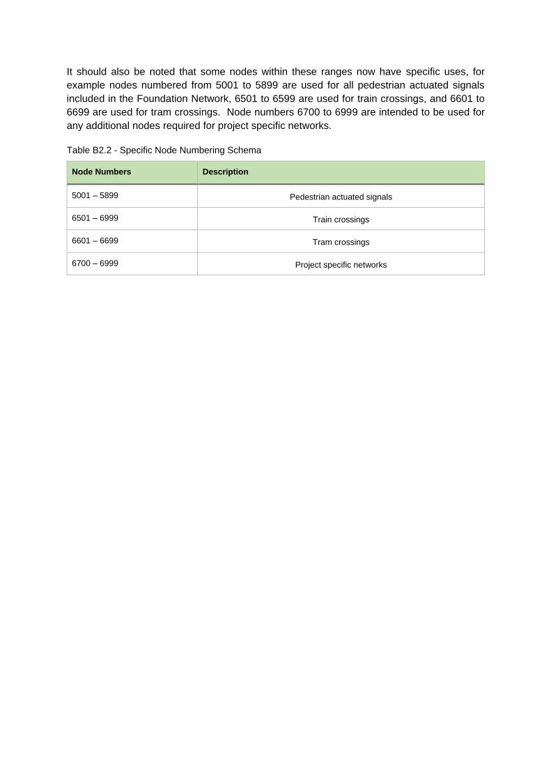
It should also be noted that some nodes within these ranges now have specific uses, for
example nodes numbered from 5001 to 5899 are used for all pedestrian actuated signals
included in the Foundation Network, 6501 to 6599 are used for train crossings, and 6601 to
6699 are used for tram crossings. Node numbers 6700 to 6999 are intended to be used for
any additional nodes required for project specific networks.
Node Numbers Description
5001 – 5899 Pedestrian actuated signals
6501 – 6999 Train crossings
6601 – 6699 Tram crossings
6700 – 6999 Project specific networks
Table B2.2 - Specific Node Numbering Schema

B.3: Foundation Network Node and Link Attribute Definitions
B.3.1 Link Distance
It is important that the link distance is uniformly applied. All link distances have been copied
from the link shape file and have been calculated within ArcGIS using the GDA 1994 MGA
Zone 54 co-ordinate system with transverse Mercator projection. Particularly for curvilinear
links this gives quite different link distances that the default CUBE calculated distance. It is
necessary that all new / modified link distances are calculated in the same way. To simplify
this process a copy of an ArcGIS *.mxd file containing the DPTI road centreline database and
the MASTEM V3 shape file has been provided. This can be accessed from program 3 of the
Prepare Data Files application.
B.3.2 Node and Link Reporting Tool Attributes
The node attributes NODE_TYPE, NODE_JC, NODE_HWSEC, NODE_PTSEC,
NODE_RF_{Year} are defined in Tables B.3, B.5, B 6, B.7 and B.9 respectively, with the link
attributes LINK_TYPE, LINK_JC, LINK_HWSEC, LINK_PTSEC, LINK_HWTT,
LINK_RF_{Year} and SL_NUM being defined in Tables B.4, B.5, B.6, B.7, B.8, B.9 and B.10
respectively. All of these attributes are used by the MASTEM Reporting Tool to ensure that
the various reports are generated consistently for different scenarios.
NODE_TYPE Description
1 Traffic Activity Zone
2 Signalised Intersection / Junction
3 Pedestrian Crossing
4 Train Crossing
5 Tram Crossing
6 Roundabout
7 Priority Intersection / Junction
8 Mid-block
10 Train Stations
20 Tram Stops
Table B3 - Foundation Network Node Definitions
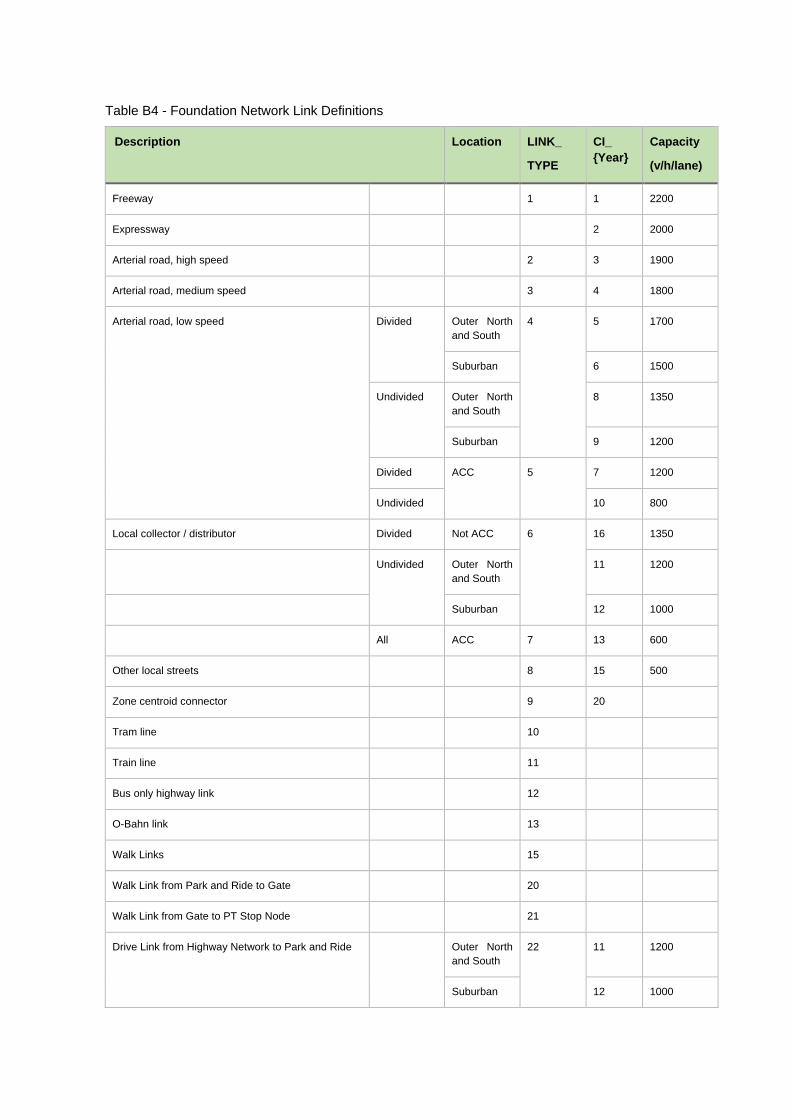
Description Location LINK_
TYPE
CI_
{Year}
Capacity
(v/h/lane)
Freeway 1 1 2200
Expressway 2 2000
Arterial road, high speed 2 3 1900
Arterial road, medium speed 3 4 1800
Arterial road, low speed Divided Outer North
and South
4 5 1700
Suburban 6 1500
Undivided Outer North
and South
8 1350
Suburban 9 1200
Divided ACC 5 7 1200
Undivided 10 800
Local collector / distributor Divided Not ACC 6 16 1350
Undivided Outer North
and South
11 1200
Suburban 12 1000
All ACC 7 13 600
Other local streets 8 15 500
Zone centroid connector 9 20
Tram line 10
Train line 11
Bus only highway link 12
O-Bahn link 13
Walk Links 15
Walk Link from Park and Ride to Gate 20
Walk Link from Gate to PT Stop Node 21
Drive Link from Highway Network to Park and Ride Outer North
and South
22 11 1200
Suburban 12 1000
Table B4 - Foundation Network Link Definitions
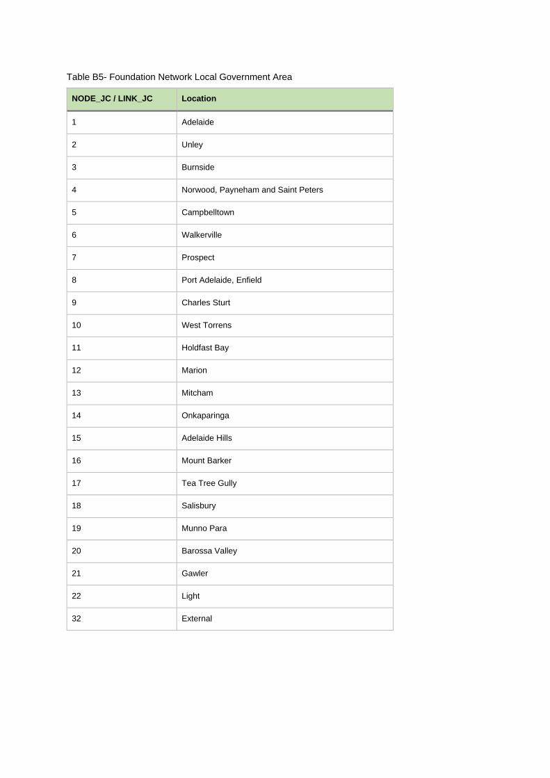
NODE_JC / LINK_JC Location
1 Adelaide
2 Unley
3 Burnside
4 Norwood, Payneham and Saint Peters
5 Campbelltown
6 Walkerville
7 Prospect
8 Port Adelaide, Enfield
9 Charles Sturt
10 West Torrens
11 Holdfast Bay
12 Marion
13 Mitcham
14 Onkaparinga
15 Adelaide Hills
16 Mount Barker
17 Tea Tree Gully
18 Salisbury
19 Munno Para
20 Barossa Valley
21 Gawler
22 Light
32 External
Table B5- Foundation Network Local Government Area
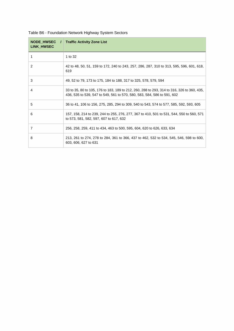
NODE_HWSEC /
LINK_HWSEC
Traffic Activity Zone List
1 1 to 32
2 42 to 48, 50, 51, 159 to 172, 240 to 243, 257, 286, 287, 310 to 313, 595, 596, 601, 618,
619
3 49, 52 to 79, 173 to 175, 184 to 188, 317 to 325, 578, 579, 594
4 33 to 35, 80 to 105, 176 to 183, 189 to 212, 260, 288 to 293, 314 to 316, 326 to 360, 435,
436, 535 to 539, 547 to 549, 561 to 570, 580, 583, 584, 586 to 591, 602
5 36 to 41, 106 to 156, 275, 285, 294 to 309, 540 to 543, 574 to 577, 585, 592, 593, 605
6 157, 158, 214 to 239, 244 to 255, 276, 277, 367 to 410, 501 to 531, 544, 550 to 560, 571
to 573, 581, 582, 597, 607 to 617, 632
7 256, 258, 259, 411 to 434, 463 to 500, 595, 604, 620 to 626, 633, 634
8 213, 261 to 274, 278 to 284, 361 to 366, 437 to 462, 532 to 534, 545, 546, 598 to 600,
603, 606, 627 to 631
Table B6 - Foundation Network Highway System Sectors
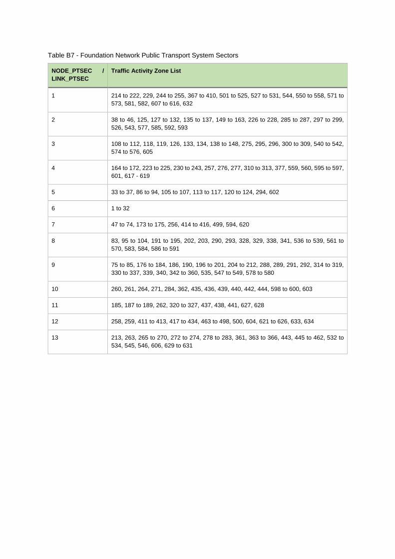
NODE_PTSEC /
LINK_PTSEC
Traffic Activity Zone List
1 214 to 222, 229, 244 to 255, 367 to 410, 501 to 525, 527 to 531, 544, 550 to 558, 571 to
573, 581, 582, 607 to 616, 632
2 38 to 46, 125, 127 to 132, 135 to 137, 149 to 163, 226 to 228, 285 to 287, 297 to 299,
526, 543, 577, 585, 592, 593
3 108 to 112, 118, 119, 126, 133, 134, 138 to 148, 275, 295, 296, 300 to 309, 540 to 542,
574 to 576, 605
4 164 to 172, 223 to 225, 230 to 243, 257, 276, 277, 310 to 313, 377, 559, 560, 595 to 597,
601, 617 - 619
5 33 to 37, 86 to 94, 105 to 107, 113 to 117, 120 to 124, 294, 602
6 1 to 32
7 47 to 74, 173 to 175, 256, 414 to 416, 499, 594, 620
8 83, 95 to 104, 191 to 195, 202, 203, 290, 293, 328, 329, 338, 341, 536 to 539, 561 to
570, 583, 584, 586 to 591
9 75 to 85, 176 to 184, 186, 190, 196 to 201, 204 to 212, 288, 289, 291, 292, 314 to 319,
330 to 337, 339, 340, 342 to 360, 535, 547 to 549, 578 to 580
10 260, 261, 264, 271, 284, 362, 435, 436, 439, 440, 442, 444, 598 to 600, 603
11 185, 187 to 189, 262, 320 to 327, 437, 438, 441, 627, 628
12 258, 259, 411 to 413, 417 to 434, 463 to 498, 500, 604, 621 to 626, 633, 634
13 213, 263, 265 to 270, 272 to 274, 278 to 283, 361, 363 to 366, 443, 445 to 462, 532 to
534, 545, 546, 606, 629 to 631
Table B7 - Foundation Network Public Transport System Sectors
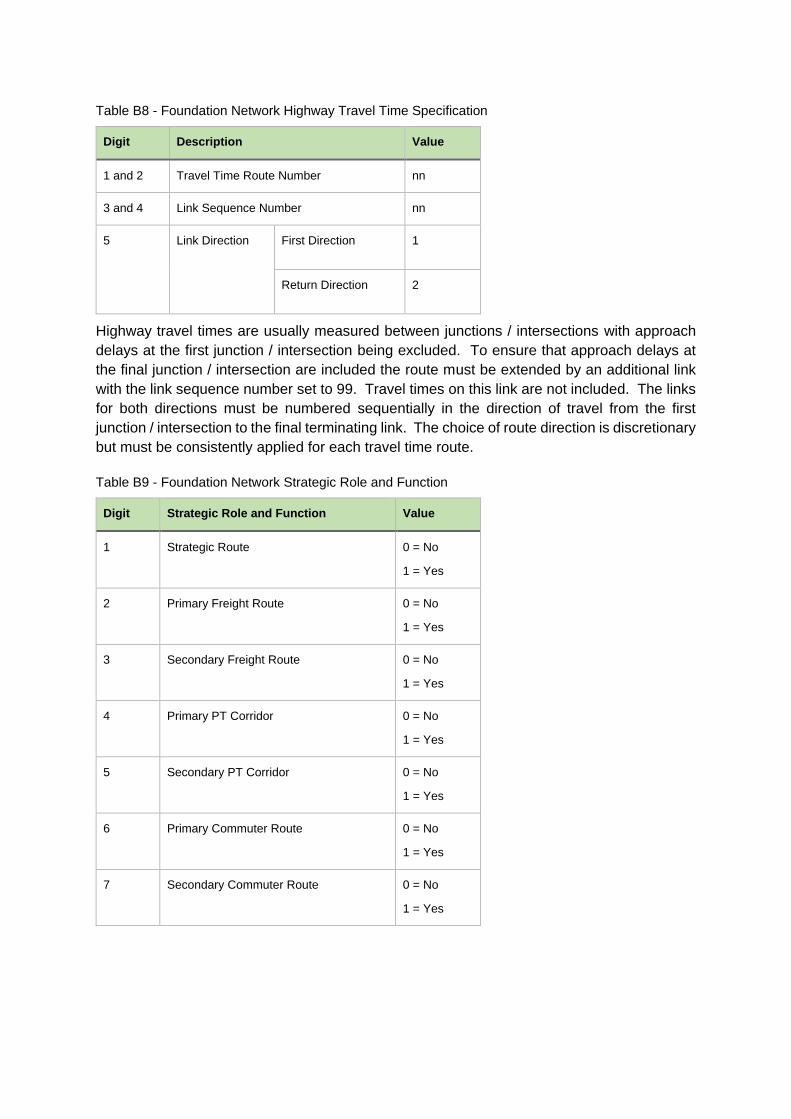
Digit Description Value
1 and 2 Travel Time Route Number nn
3 and 4 Link Sequence Number nn
5 Link Direction First Direction 1
Return Direction 2
Highway travel times are usually measured between junctions / intersections with approach
delays at the first junction / intersection being excluded. To ensure that approach delays at
the final junction / intersection are included the route must be extended by an additional link
with the link sequence number set to 99. Travel times on this link are not included. The links
for both directions must be numbered sequentially in the direction of travel from the first
junction / intersection to the final terminating link. The choice of route direction is discretionary
but must be consistently applied for each travel time route.
Digit Strategic Role and Function Value
1 Strategic Route 0 = No
1 = Yes
2 Primary Freight Route 0 = No
1 = Yes
3 Secondary Freight Route 0 = No
1 = Yes
4 Primary PT Corridor 0 = No
1 = Yes
5 Secondary PT Corridor 0 = No
1 = Yes
6 Primary Commuter Route 0 = No
1 = Yes
7 Secondary Commuter Route 0 = No
1 = Yes
Table B8 - Foundation Network Highway Travel Time Specification
Table B9 - Foundation Network Strategic Role and Function
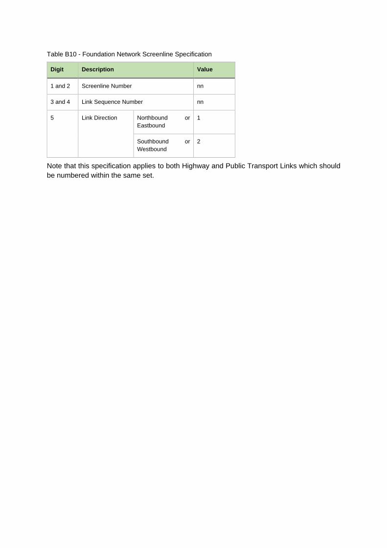
Digit Description Value
1 and 2 Screenline Number nn
3 and 4 Link Sequence Number nn
5 Link Direction Northbound or
Eastbound
1
Southbound or
Westbound
2
Note that this specification applies to both Highway and Public Transport Links which should
be numbered within the same set.
Table B10 - Foundation Network Screenline Specification
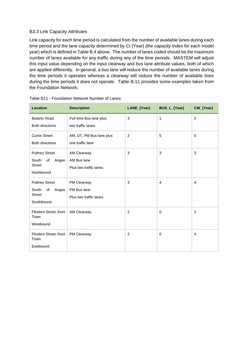
B3.3 Link Capacity Attributes
Link capacity for each time period is calculated from the number of available lanes during each
time period and the lane capacity determined by CI {Year} (the capacity Index for each model
year) which is defined in Table B.4 above. The number of lanes coded should be the maximum
number of lanes available for any traffic during any of the time periods. MASTEM will adjust
this input value depending on the input clearway and bus lane attribute values, both of which
are applied differently. In general, a bus lane will reduce the number of available lanes during
the time periods it operates whereas a clearway will reduce the number of available lines
during the time periods it does not operate. Table B.11 provides some examples taken from
the Foundation Network.
Location Description LANE_{Year} BUS_L_{Year} CW_{Year}
Botanic Road
Both directions
Full time Bus lane plus
two traffic lanes
3 1 0
Currie Street
Both directions
AM, DT, PM Bus lane plus
one traffic lane
2 5 0
Pultney Street
South of Angas
Street
Northbound
AM Clearway
AM Bus lane
Plus two traffic lanes
3 3 3
Pultney Street
South of Angas
Street
Southbound
PM Clearway
PM Bus lane
Plus two traffic lanes
3 4 4
Flinders Street, Kent
Town
Westbound
AM Clearway 2 0 3
Flinders Street, Kent
Town
Eastbound
PM Clearway 2 0 4
Table B11 - Foundation Network Number of Lanes
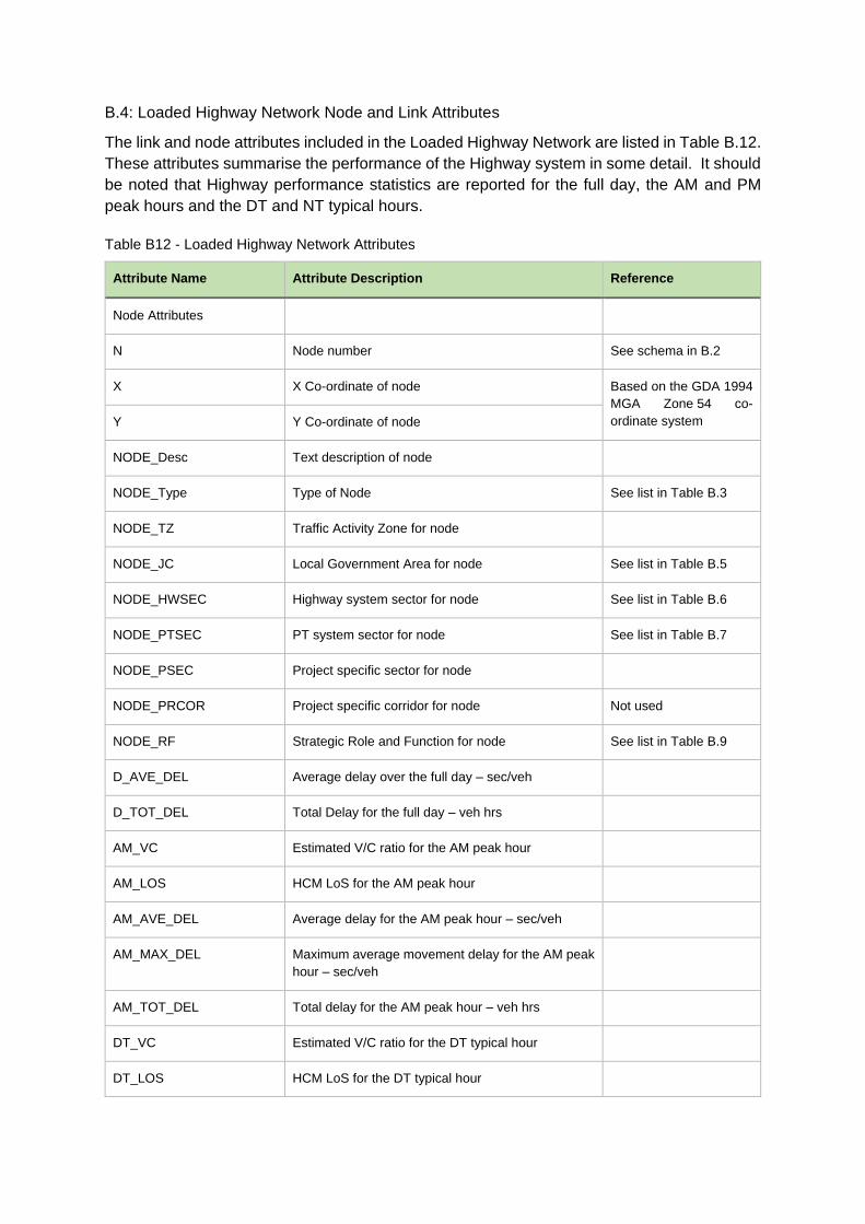
B.4: Loaded Highway Network Node and Link Attributes
The link and node attributes included in the Loaded Highway Network are listed in Table B.12.
These attributes summarise the performance of the Highway system in some detail. It should
be noted that Highway performance statistics are reported for the full day, the AM and PM
peak hours and the DT and NT typical hours.
Attribute Name Attribute Description Reference
Node Attributes
N Node number See schema in B.2
X X Co-ordinate of node Based on the GDA 1994
MGA Zone 54 co-
ordinate system Y Y Co-ordinate of node
NODE_Desc Text description of node
NODE_Type Type of Node See list in Table B.3
NODE_TZ Traffic Activity Zone for node
NODE_JC Local Government Area for node See list in Table B.5
NODE_HWSEC Highway system sector for node See list in Table B.6
NODE_PTSEC PT system sector for node See list in Table B.7
NODE_PSEC Project specific sector for node
NODE_PRCOR Project specific corridor for node Not used
NODE_RF Strategic Role and Function for node See list in Table B.9
D_AVE_DEL Average delay over the full day – sec/veh
D_TOT_DEL Total Delay for the full day – veh hrs
AM_VC Estimated V/C ratio for the AM peak hour
AM_LOS HCM LoS for the AM peak hour
AM_AVE_DEL Average delay for the AM peak hour – sec/veh
AM_MAX_DEL Maximum average movement delay for the AM peak
hour – sec/veh
AM_TOT_DEL Total delay for the AM peak hour – veh hrs
DT_VC Estimated V/C ratio for the DT typical hour
DT_LOS HCM LoS for the DT typical hour
Table B12 - Loaded Highway Network Attributes
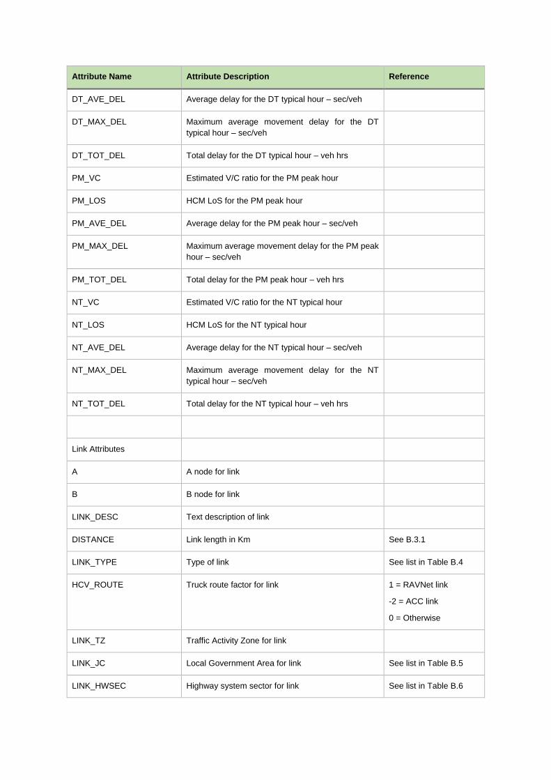
Attribute Name Attribute Description Reference
DT_AVE_DEL Average delay for the DT typical hour – sec/veh
DT_MAX_DEL Maximum average movement delay for the DT
typical hour – sec/veh
DT_TOT_DEL Total delay for the DT typical hour – veh hrs
PM_VC Estimated V/C ratio for the PM peak hour
PM_LOS HCM LoS for the PM peak hour
PM_AVE_DEL Average delay for the PM peak hour – sec/veh
PM_MAX_DEL Maximum average movement delay for the PM peak
hour – sec/veh
PM_TOT_DEL Total delay for the PM peak hour – veh hrs
NT_VC Estimated V/C ratio for the NT typical hour
NT_LOS HCM LoS for the NT typical hour
NT_AVE_DEL Average delay for the NT typical hour – sec/veh
NT_MAX_DEL Maximum average movement delay for the NT
typical hour – sec/veh
NT_TOT_DEL Total delay for the NT typical hour – veh hrs
Link Attributes
A A node for link
B B node for link
LINK_DESC Text description of link
DISTANCE Link length in Km See B.3.1
LINK_TYPE Type of link See list in Table B.4
HCV_ROUTE Truck route factor for link 1 = RAVNet link
-2 = ACC link
0 = Otherwise
LINK_TZ Traffic Activity Zone for link
LINK_JC Local Government Area for link See list in Table B.5
LINK_HWSEC Highway system sector for link See list in Table B.6
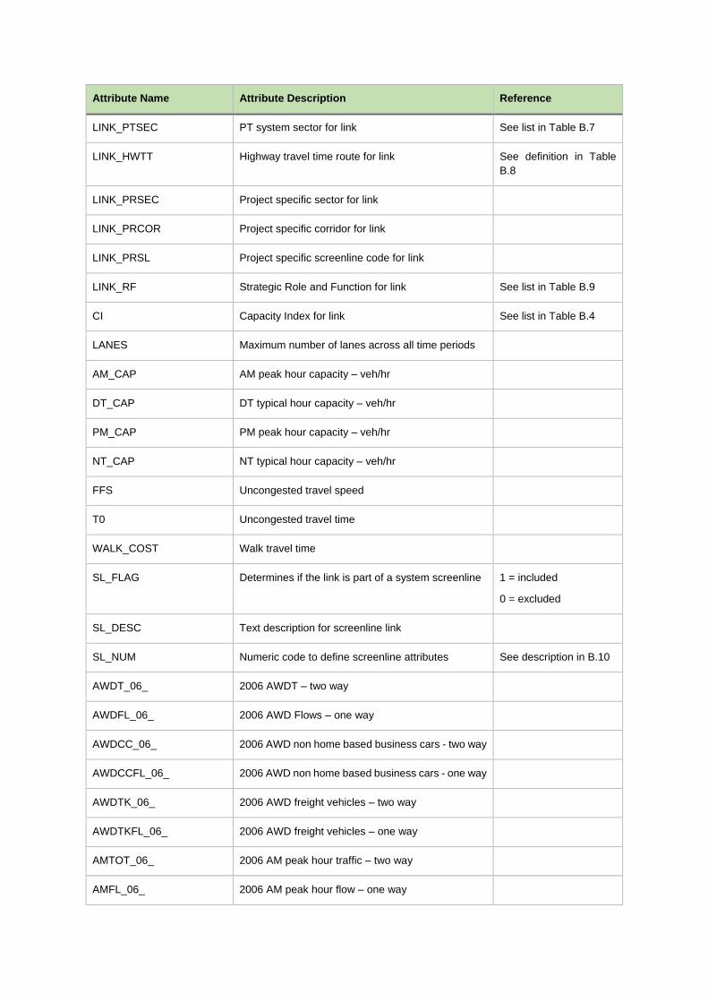
Attribute Name Attribute Description Reference
LINK_PTSEC PT system sector for link See list in Table B.7
LINK_HWTT Highway travel time route for link See definition in Table
B.8
LINK_PRSEC Project specific sector for link
LINK_PRCOR Project specific corridor for link
LINK_PRSL Project specific screenline code for link
LINK_RF Strategic Role and Function for link See list in Table B.9
CI Capacity Index for link See list in Table B.4
LANES Maximum number of lanes across all time periods
AM_CAP AM peak hour capacity – veh/hr
DT_CAP DT typical hour capacity – veh/hr
PM_CAP PM peak hour capacity – veh/hr
NT_CAP NT typical hour capacity – veh/hr
FFS Uncongested travel speed
T0 Uncongested travel time
WALK_COST Walk travel time
SL_FLAG Determines if the link is part of a system screenline 1 = included
0 = excluded
SL_DESC Text description for screenline link
SL_NUM Numeric code to define screenline attributes See description in B.10
AWDT_06_ 2006 AWDT – two way
AWDFL_06_ 2006 AWD Flows – one way
AWDCC_06_ 2006 AWD non home based business cars - two way
AWDCCFL_06_ 2006 AWD non home based business cars - one way
AWDTK_06_ 2006 AWD freight vehicles – two way
AWDTKFL_06_ 2006 AWD freight vehicles – one way
AMTOT_06_ 2006 AM peak hour traffic – two way
AMFL_06_ 2006 AM peak hour flow – one way
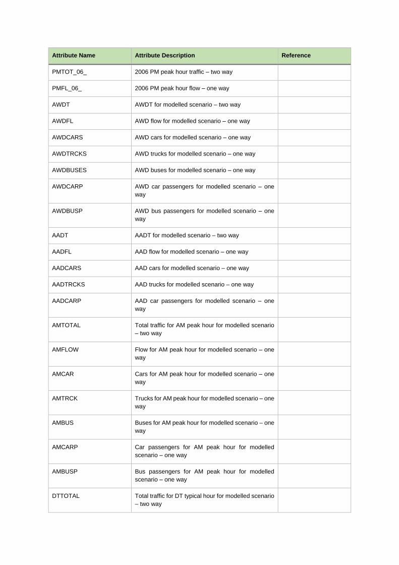
Attribute Name Attribute Description Reference
PMTOT_06_ 2006 PM peak hour traffic – two way
PMFL_06_ 2006 PM peak hour flow – one way
AWDT AWDT for modelled scenario – two way
AWDFL AWD flow for modelled scenario – one way
AWDCARS AWD cars for modelled scenario – one way
AWDTRCKS AWD trucks for modelled scenario – one way
AWDBUSES AWD buses for modelled scenario – one way
AWDCARP AWD car passengers for modelled scenario – one
way
AWDBUSP AWD bus passengers for modelled scenario – one
way
AADT AADT for modelled scenario – two way
AADFL AAD flow for modelled scenario – one way
AADCARS AAD cars for modelled scenario – one way
AADTRCKS AAD trucks for modelled scenario – one way
AADCARP AAD car passengers for modelled scenario – one
way
AMTOTAL Total traffic for AM peak hour for modelled scenario
– two way
AMFLOW Flow for AM peak hour for modelled scenario – one
way
AMCAR Cars for AM peak hour for modelled scenario – one
way
AMTRCK Trucks for AM peak hour for modelled scenario – one
way
AMBUS Buses for AM peak hour for modelled scenario – one
way
AMCARP Car passengers for AM peak hour for modelled
scenario – one way
AMBUSP Bus passengers for AM peak hour for modelled
scenario – one way
DTTOTAL Total traffic for DT typical hour for modelled scenario
– two way
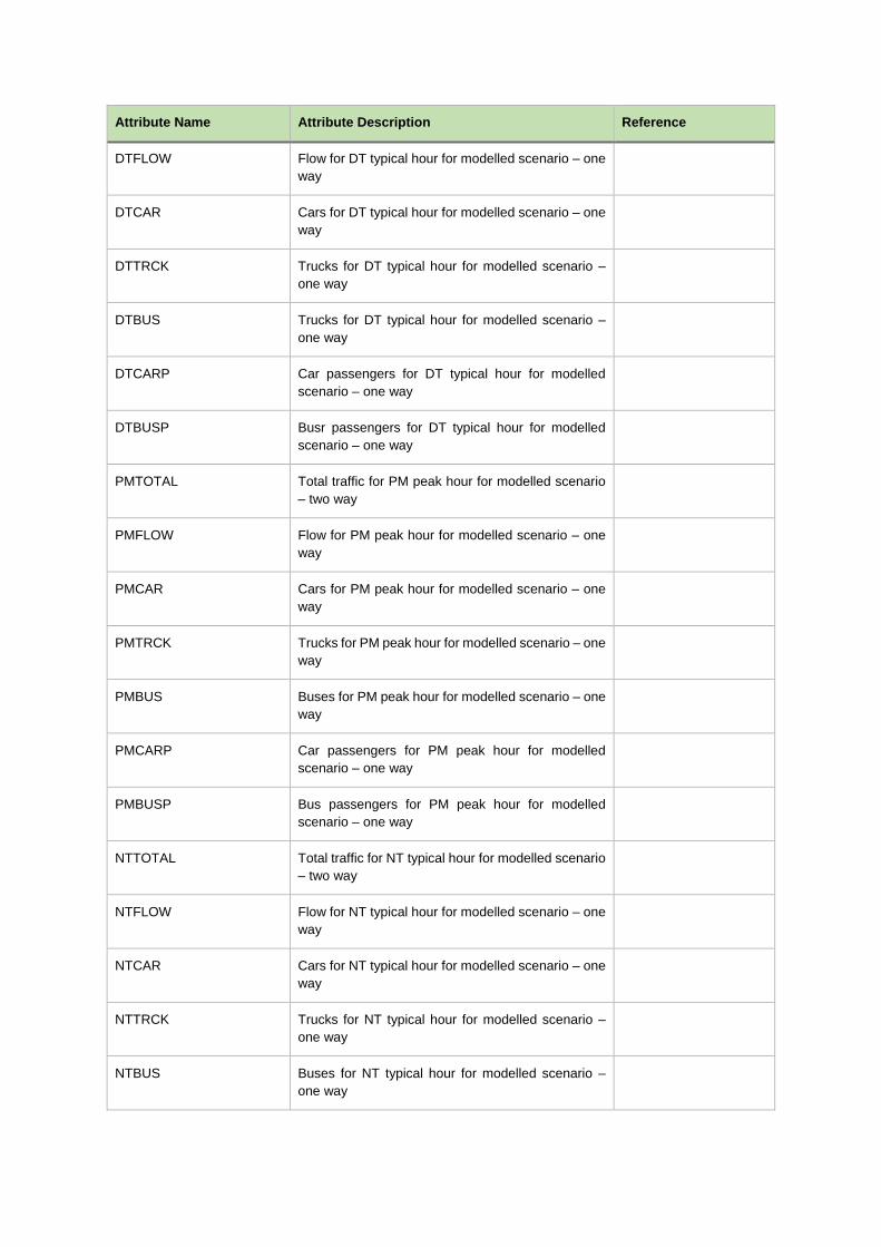
Attribute Name Attribute Description Reference
DTFLOW Flow for DT typical hour for modelled scenario – one
way
DTCAR Cars for DT typical hour for modelled scenario – one
way
DTTRCK Trucks for DT typical hour for modelled scenario –
one way
DTBUS Trucks for DT typical hour for modelled scenario –
one way
DTCARP Car passengers for DT typical hour for modelled
scenario – one way
DTBUSP Busr passengers for DT typical hour for modelled
scenario – one way
PMTOTAL Total traffic for PM peak hour for modelled scenario
– two way
PMFLOW Flow for PM peak hour for modelled scenario – one
way
PMCAR Cars for PM peak hour for modelled scenario – one
way
PMTRCK Trucks for PM peak hour for modelled scenario – one
way
PMBUS Buses for PM peak hour for modelled scenario – one
way
PMCARP Car passengers for PM peak hour for modelled
scenario – one way
PMBUSP Bus passengers for PM peak hour for modelled
scenario – one way
NTTOTAL Total traffic for NT typical hour for modelled scenario
– two way
NTFLOW Flow for NT typical hour for modelled scenario – one
way
NTCAR Cars for NT typical hour for modelled scenario – one
way
NTTRCK Trucks for NT typical hour for modelled scenario –
one way
NTBUS Buses for NT typical hour for modelled scenario –
one way
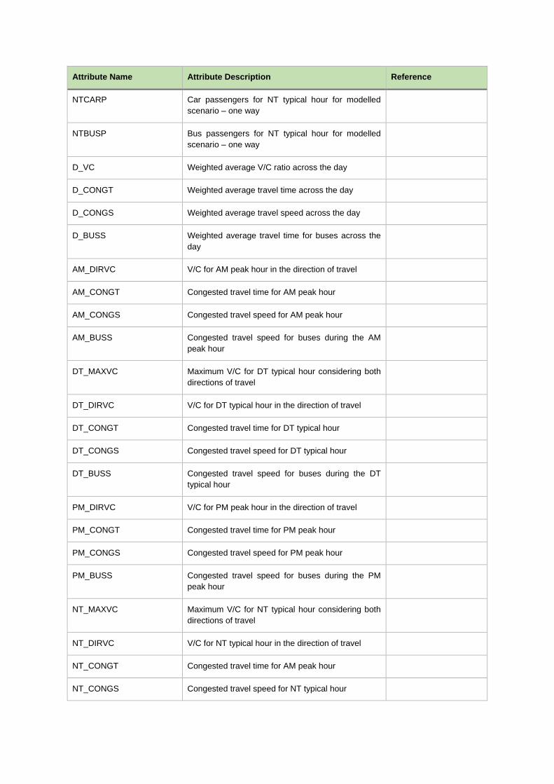
Attribute Name Attribute Description Reference
NTCARP Car passengers for NT typical hour for modelled
scenario – one way
NTBUSP Bus passengers for NT typical hour for modelled
scenario – one way
D_VC Weighted average V/C ratio across the day
D_CONGT Weighted average travel time across the day
D_CONGS Weighted average travel speed across the day
D_BUSS Weighted average travel time for buses across the
day
AM_DIRVC V/C for AM peak hour in the direction of travel
AM_CONGT Congested travel time for AM peak hour
AM_CONGS Congested travel speed for AM peak hour
AM_BUSS Congested travel speed for buses during the AM
peak hour
DT_MAXVC Maximum V/C for DT typical hour considering both
directions of travel
DT_DIRVC V/C for DT typical hour in the direction of travel
DT_CONGT Congested travel time for DT typical hour
DT_CONGS Congested travel speed for DT typical hour
DT_BUSS Congested travel speed for buses during the DT
typical hour
PM_DIRVC V/C for PM peak hour in the direction of travel
PM_CONGT Congested travel time for PM peak hour
PM_CONGS Congested travel speed for PM peak hour
PM_BUSS Congested travel speed for buses during the PM
peak hour
NT_MAXVC Maximum V/C for NT typical hour considering both
directions of travel
NT_DIRVC V/C for NT typical hour in the direction of travel
NT_CONGT Congested travel time for AM peak hour
NT_CONGS Congested travel speed for NT typical hour
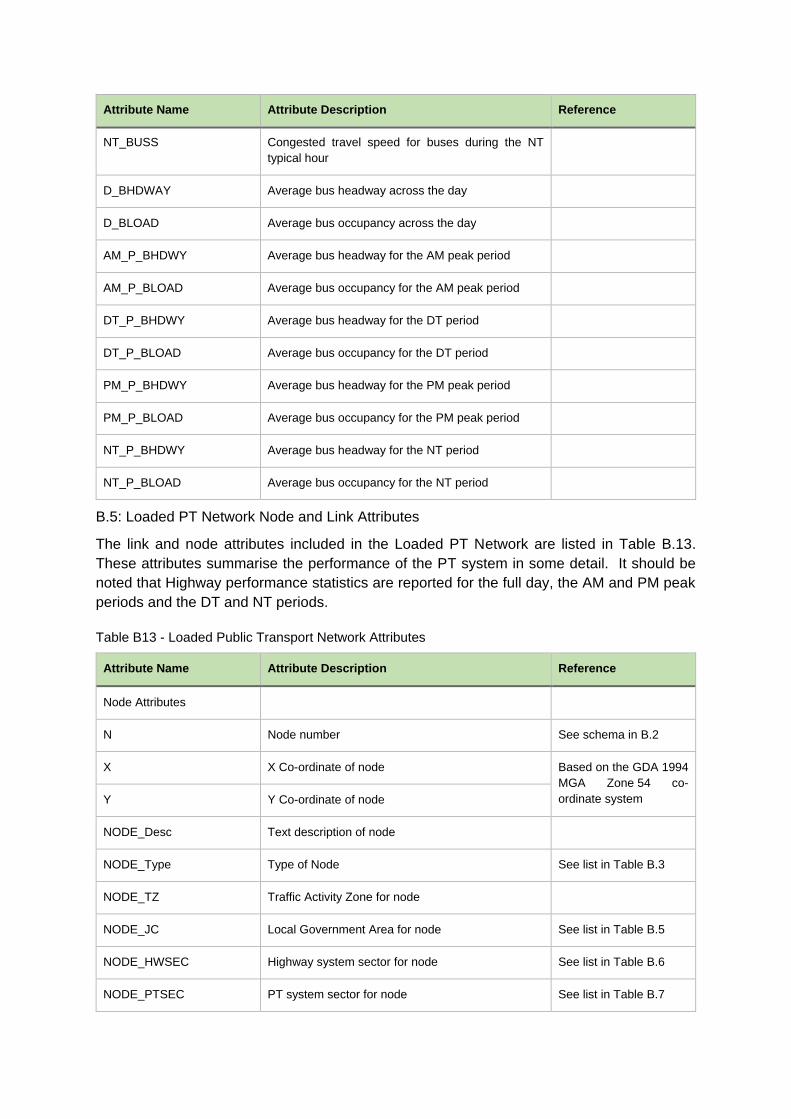
Attribute Name Attribute Description Reference
NT_BUSS Congested travel speed for buses during the NT
typical hour
D_BHDWAY Average bus headway across the day
D_BLOAD Average bus occupancy across the day
AM_P_BHDWY Average bus headway for the AM peak period
AM_P_BLOAD Average bus occupancy for the AM peak period
DT_P_BHDWY Average bus headway for the DT period
DT_P_BLOAD Average bus occupancy for the DT period
PM_P_BHDWY Average bus headway for the PM peak period
PM_P_BLOAD Average bus occupancy for the PM peak period
NT_P_BHDWY Average bus headway for the NT period
NT_P_BLOAD Average bus occupancy for the NT period
B.5: Loaded PT Network Node and Link Attributes
The link and node attributes included in the Loaded PT Network are listed in Table B.13.
These attributes summarise the performance of the PT system in some detail. It should be
noted that Highway performance statistics are reported for the full day, the AM and PM peak
periods and the DT and NT periods.
Attribute Name Attribute Description Reference
Node Attributes
N Node number See schema in B.2
X X Co-ordinate of node Based on the GDA 1994
MGA Zone 54 co-
ordinate system Y Y Co-ordinate of node
NODE_Desc Text description of node
NODE_Type Type of Node See list in Table B.3
NODE_TZ Traffic Activity Zone for node
NODE_JC Local Government Area for node See list in Table B.5
NODE_HWSEC Highway system sector for node See list in Table B.6
NODE_PTSEC PT system sector for node See list in Table B.7
Table B13 - Loaded Public Transport Network Attributes
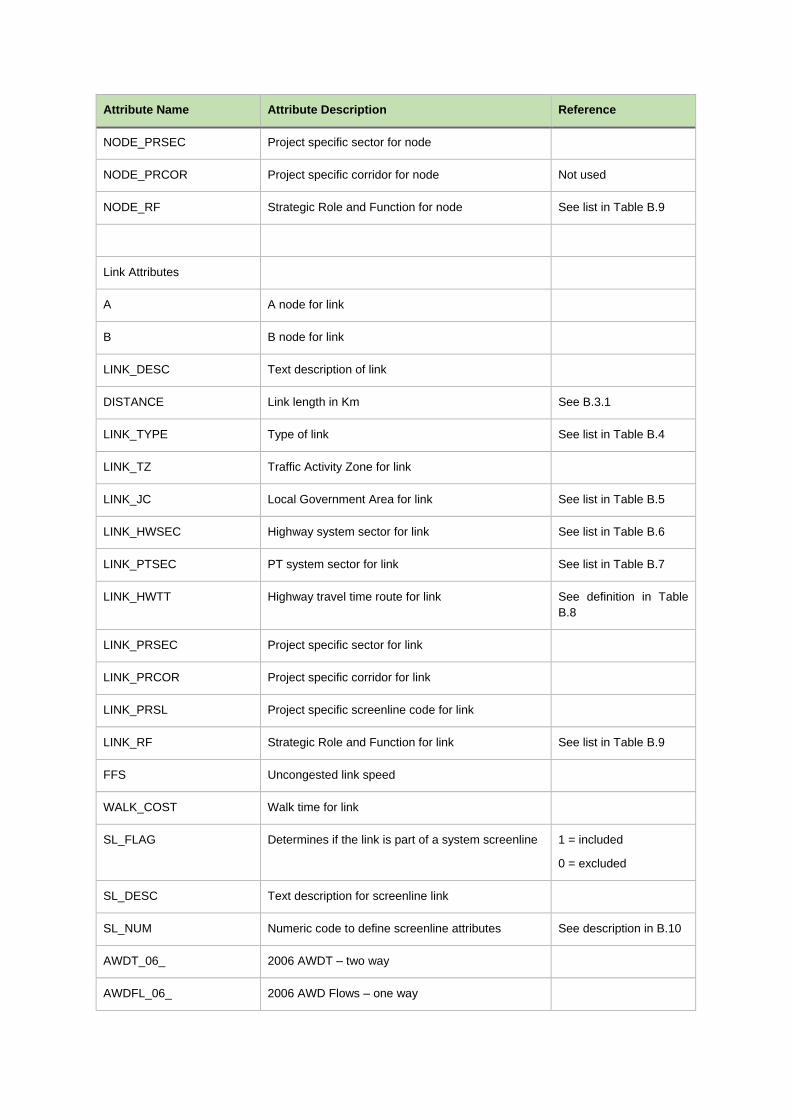
Attribute Name Attribute Description Reference
NODE_PRSEC Project specific sector for node
NODE_PRCOR Project specific corridor for node Not used
NODE_RF Strategic Role and Function for node See list in Table B.9
Link Attributes
A A node for link
B B node for link
LINK_DESC Text description of link
DISTANCE Link length in Km See B.3.1
LINK_TYPE Type of link See list in Table B.4
LINK_TZ Traffic Activity Zone for link
LINK_JC Local Government Area for link See list in Table B.5
LINK_HWSEC Highway system sector for link See list in Table B.6
LINK_PTSEC PT system sector for link See list in Table B.7
LINK_HWTT Highway travel time route for link See definition in Table
B.8
LINK_PRSEC Project specific sector for link
LINK_PRCOR Project specific corridor for link
LINK_PRSL Project specific screenline code for link
LINK_RF Strategic Role and Function for link See list in Table B.9
FFS Uncongested link speed
WALK_COST Walk time for link
SL_FLAG Determines if the link is part of a system screenline 1 = included
0 = excluded
SL_DESC Text description for screenline link
SL_NUM Numeric code to define screenline attributes See description in B.10
AWDT_06_ 2006 AWDT – two way
AWDFL_06_ 2006 AWD Flows – one way
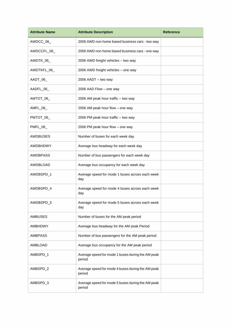
Attribute Name Attribute Description Reference
AWDCC_06_ 2006 AWD non home based business cars - two way
AWDCCFL_06_ 2006 AWD non home based business cars - one way
AWDTK_06_ 2006 AWD freight vehicles – two way
AWDTKFL_06_ 2006 AWD freight vehicles – one way
AADT_06_ 2006 AADT – two way
AADFL_06_ 2006 AAD Flow – one way
AMTOT_06_ 2006 AM peak hour traffic – two way
AMFL_06_ 2006 AM peak hour flow – one way
PMTOT_06_ 2006 PM peak hour traffic – two way
PMFL_06_ 2006 PM peak hour flow – one way
AWDBUSES Number of buses for each week day
AWDBHDWY Average bus headway for each week day
AWDBPASS Number of bus passengers for each week day
AWDBLOAD Average bus occupancy for each week day
AWDBSPD_1 Average speed for mode 1 buses across each week
day
AWDBSPD_4 Average speed for mode 4 buses across each week
day
AWDBSPD_5 Average speed for mode 5 buses across each week
day
AMBUSES Number of buses for the AM peak period
AMBHDWY Average bus headway for the AM peak Period
AMBPASS Number of bus passengers for the AM peak period
AMBLOAD Average bus occupancy for the AM peak period
AMBSPD_1 Average speed for mode 1 buses during the AM peak
period
AMBSPD_2 Average speed for mode 4 buses during the AM peak
period
AMBSPD_3 Average speed for mode 5 buses during the AM peak
period
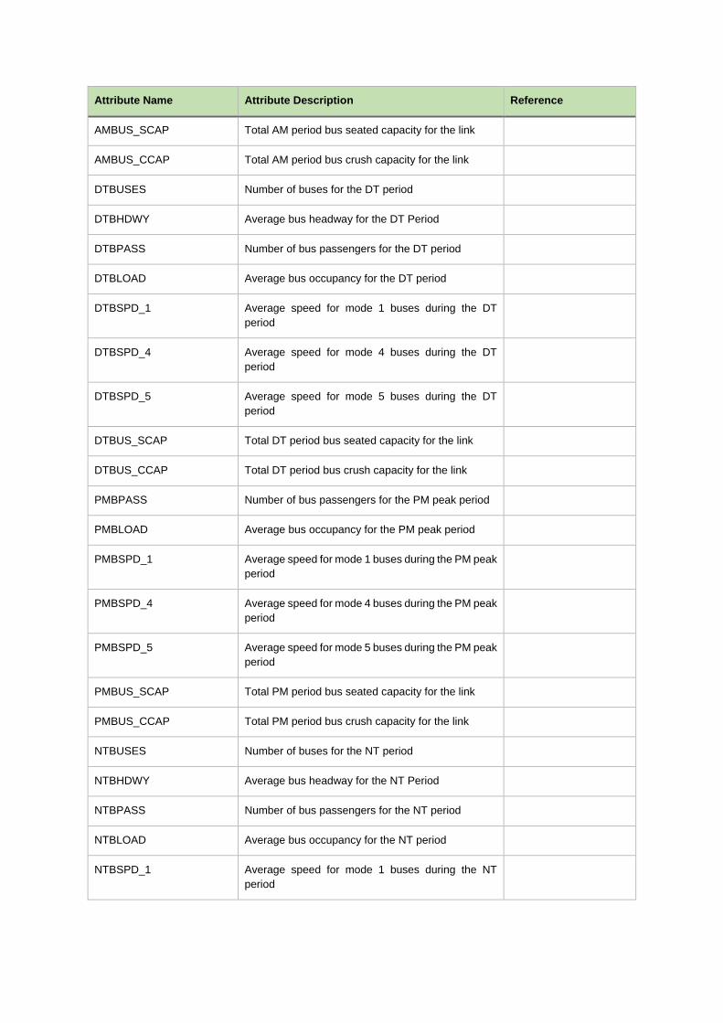
Attribute Name Attribute Description Reference
AMBUS_SCAP Total AM period bus seated capacity for the link
AMBUS_CCAP Total AM period bus crush capacity for the link
DTBUSES Number of buses for the DT period
DTBHDWY Average bus headway for the DT Period
DTBPASS Number of bus passengers for the DT period
DTBLOAD Average bus occupancy for the DT period
DTBSPD_1 Average speed for mode 1 buses during the DT
period
DTBSPD_4 Average speed for mode 4 buses during the DT
period
DTBSPD_5 Average speed for mode 5 buses during the DT
period
DTBUS_SCAP Total DT period bus seated capacity for the link
DTBUS_CCAP Total DT period bus crush capacity for the link
PMBPASS Number of bus passengers for the PM peak period
PMBLOAD Average bus occupancy for the PM peak period
PMBSPD_1 Average speed for mode 1 buses during the PM peak
period
PMBSPD_4 Average speed for mode 4 buses during the PM peak
period
PMBSPD_5 Average speed for mode 5 buses during the PM peak
period
PMBUS_SCAP Total PM period bus seated capacity for the link
PMBUS_CCAP Total PM period bus crush capacity for the link
NTBUSES Number of buses for the NT period
NTBHDWY Average bus headway for the NT Period
NTBPASS Number of bus passengers for the NT period
NTBLOAD Average bus occupancy for the NT period
NTBSPD_1 Average speed for mode 1 buses during the NT
period
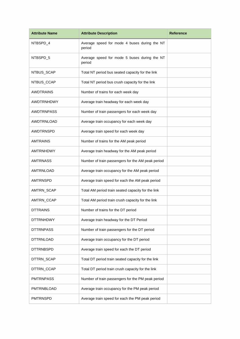
Attribute Name Attribute Description Reference
NTBSPD_4 Average speed for mode 4 buses during the NT
period
NTBSPD_5 Average speed for mode 5 buses during the NT
period
NTBUS_SCAP Total NT period bus seated capacity for the link
NTBUS_CCAP Total NT period bus crush capacity for the link
AWDTRAINS Number of trains for each week day
AWDTRNHDWY Average train headway for each week day
AWDTRNPASS Number of train passengers for each week day
AWDTRNLOAD Average train occupancy for each week day
AWDTRNSPD Average train speed for each week day
AMTRAINS Number of trains for the AM peak period
AMTRNHDWY Average train headway for the AM peak period
AMTRNASS Number of train passengers for the AM peak period
AMTRNLOAD Average train occupancy for the AM peak period
AMTRNSPD Average train speed for each the AM peak period
AMTRN_SCAP Total AM period train seated capacity for the link
AMTRN_CCAP Total AM period train crush capacity for the link
DTTRAINS Number of trains for the DT period
DTTRNHDWY Average train headway for the DT Period
DTTRNPASS Number of train passengers for the DT period
DTTRNLOAD Average train occupancy for the DT period
DTTRNBSPD Average train speed for each the DT period
DTTRN_SCAP Total DT period train seated capacity for the link
DTTRN_CCAP Total DT period train crush capacity for the link
PMTRNPASS Number of train passengers for the PM peak period
PMTRNBLOAD Average train occupancy for the PM peak period
PMTRNSPD Average train speed for each the PM peak period
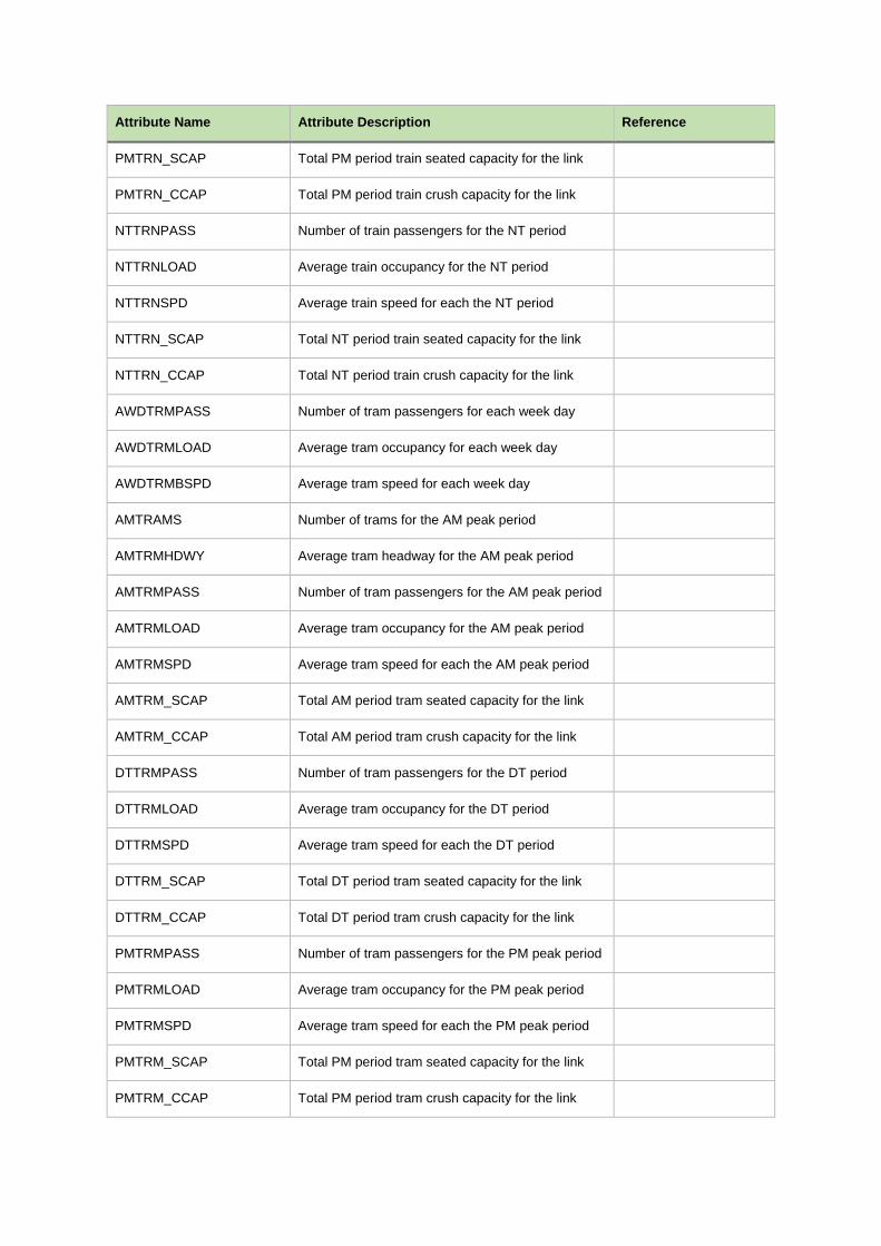
Attribute Name Attribute Description Reference
PMTRN_SCAP Total PM period train seated capacity for the link
PMTRN_CCAP Total PM period train crush capacity for the link
NTTRNPASS Number of train passengers for the NT period
NTTRNLOAD Average train occupancy for the NT period
NTTRNSPD Average train speed for each the NT period
NTTRN_SCAP Total NT period train seated capacity for the link
NTTRN_CCAP Total NT period train crush capacity for the link
AWDTRMPASS Number of tram passengers for each week day
AWDTRMLOAD Average tram occupancy for each week day
AWDTRMBSPD Average tram speed for each week day
AMTRAMS Number of trams for the AM peak period
AMTRMHDWY Average tram headway for the AM peak period
AMTRMPASS Number of tram passengers for the AM peak period
AMTRMLOAD Average tram occupancy for the AM peak period
AMTRMSPD Average tram speed for each the AM peak period
AMTRM_SCAP Total AM period tram seated capacity for the link
AMTRM_CCAP Total AM period tram crush capacity for the link
DTTRMPASS Number of tram passengers for the DT period
DTTRMLOAD Average tram occupancy for the DT period
DTTRMSPD Average tram speed for each the DT period
DTTRM_SCAP Total DT period tram seated capacity for the link
DTTRM_CCAP Total DT period tram crush capacity for the link
PMTRMPASS Number of tram passengers for the PM peak period
PMTRMLOAD Average tram occupancy for the PM peak period
PMTRMSPD Average tram speed for each the PM peak period
PMTRM_SCAP Total PM period tram seated capacity for the link
PMTRM_CCAP Total PM period tram crush capacity for the link
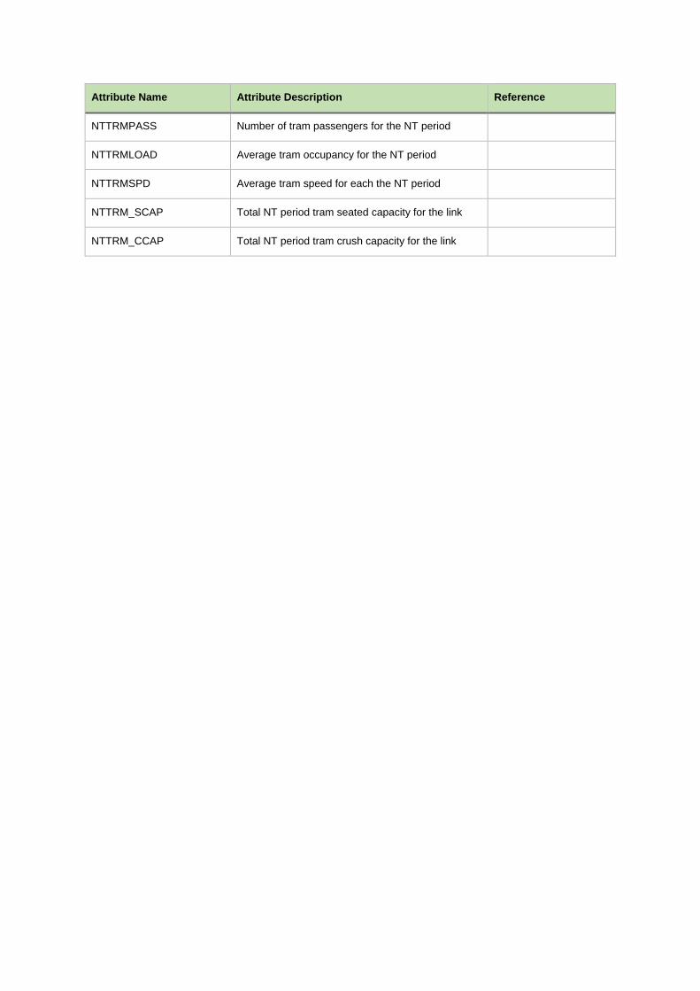
Attribute Name Attribute Description Reference
NTTRMPASS Number of tram passengers for the NT period
NTTRMLOAD Average tram occupancy for the NT period
NTTRMSPD Average tram speed for each the NT period
NTTRM_SCAP Total NT period tram seated capacity for the link
NTTRM_CCAP Total NT period tram crush capacity for the link

Appendix C – Public Transport Input Files Updating
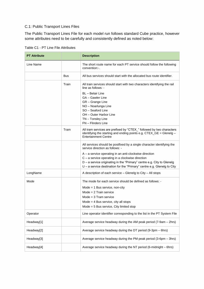
C.1: Public Transport Lines Files
The Public Transport Lines File for each model run follows standard Cube practice, however
some attributes need to be carefully and consistently defined as noted below:
PT Attribute Description
Line Name The short route name for each PT service should follow the following convention:-.
Bus All bus services should start with the allocated bus route identifier.
Train All train services should start with two characters identifying the rail line as follows: -
BL – Belair Line
GA – Gawler Line
GR – Grange Line
NO – Noarlunga Line
SO – Seaford Line
OH – Outer Harbor Line
TN – Tonsley Line
FN – Flinders Line
Tram All tram services are prefixed by “CTEX_” followed by two characters identifying the starting and ending points e.g. CTEX_GE = Glenelg – Entertainment Centre
All services should be postfixed by a single character identifying the service direction as follows: -
A – a service operating in an anti-clockwise direction
C – a service operating in a clockwise direction
D – a service originating in the “Primary” centre e.g. City to Glenelg
U – a service destination for the “Primary” centre e.g. Glenelg to City
LongName A description of each service – Glenelg to City – All stops
Mode The mode for each service should be defined as follows: -
Mode = 1 Bus service, non-city
Mode = 2 Train service
Mode = 3 Tram service
Mode = 4 Bus service, city all stops
Mode = 5 Bus service, City limited stop
Operator Line operator identifier corresponding to the list in the PT System File
Headway[1] Average service headway during the AM peak period (7-9am – 2hrs)
Headway[2] Average service headway during the DT period (9-3pm – 6hrs)
Headway[3] Average service headway during the PM peak period (3-6pm – 3hrs)
Headway[4] Average service headway during the NT period (6-midnight – 6hrs)
Table C1 - PT Line File Attributes
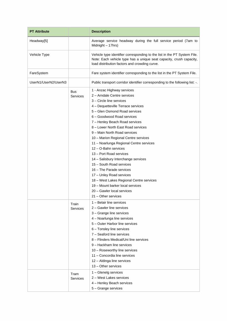
PT Attribute Description
Headway[5] Average service headway during the full service period (7am to
Midnight – 17hrs)
Vehicle Type Vehicle type identifier corresponding to the list in the PT System File.
Note: Each vehicle type has a unique seat capacity, crush capacity,
load distribution factors and crowding curve.
FareSystem Fare system identifier corresponding to the list in the PT System File.
UserN1/UserN2/UserN3 Public transport corridor identifier corresponding to the following list: -.
Bus
Services
1 - Anzac Highway services
2 – Arndale Centre services
3 – Circle line services
4 – Dequetteville Terrace services
5 – Glen Osmond Road services
6 – Goodwood Road services
7 – Henley Beach Road services
8 – Lower North East Road services
9 – Main North Road services
10 – Marion Regional Centre services
11 – Noarlunga Regional Centre services
12 – O-Bahn services
13 – Port Road services
14 – Salisbury Interchange services
15 – South Road services
16 – The Parade services
17 – Unley Road services
18 – West Lakes Regional Centre services
19 – Mount barker local services
20 – Gawler local services
21 – Other services
Train
Services
1 – Belair line services
2 – Gawler line services
3 – Grange line services
4 – Noarlunga line services
5 – Outer Harbor line services
6 – Tonsley line services
7 – Seaford line services
8 – Flinders Medical/Uni line services
9 – Hackham line services
10 – Roseworthy line services
11 – Concordia line services
12 – Aldinga line services
13 – Other services
Tram
Services
1 – Glenelg services
2 – West Lakes services
4 – Henley Beach services
5 – Grange services
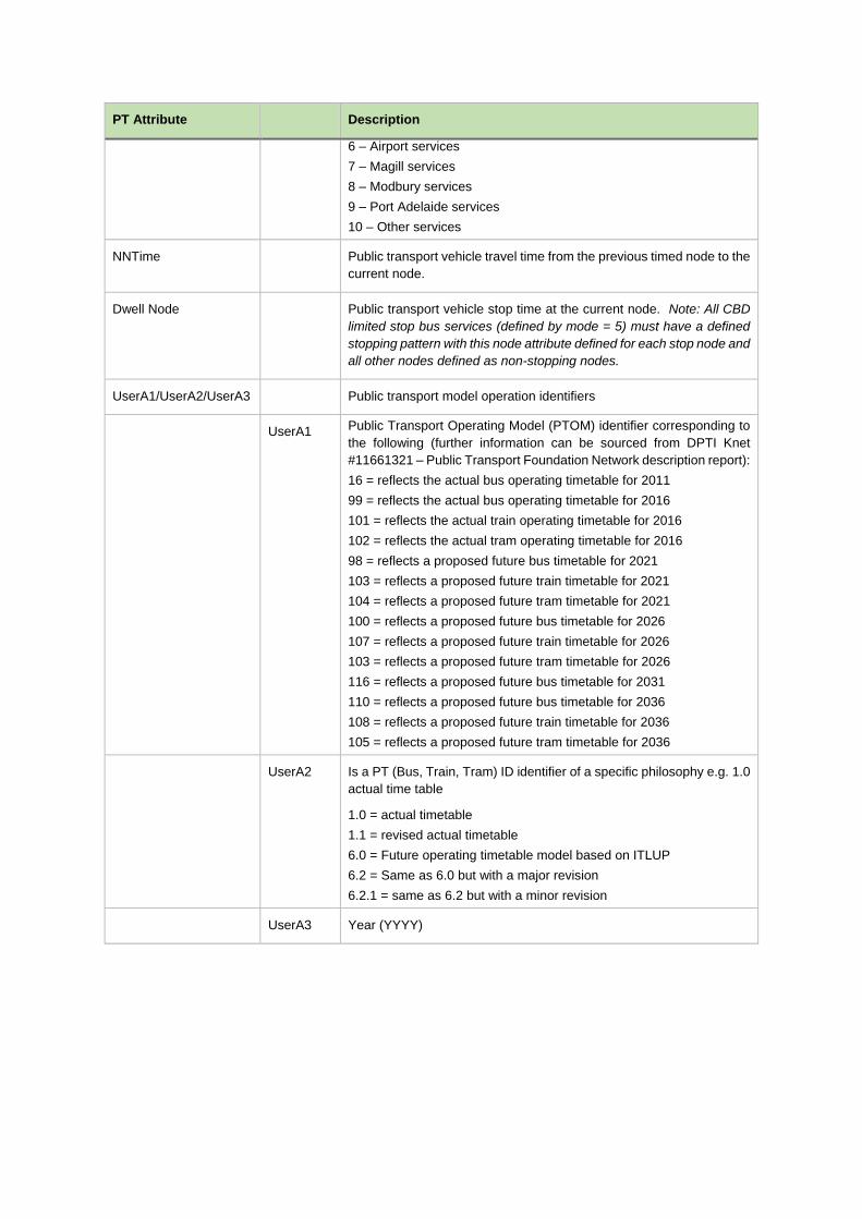
PT Attribute Description
6 – Airport services
7 – Magill services
8 – Modbury services
9 – Port Adelaide services
10 – Other services
NNTime Public transport vehicle travel time from the previous timed node to the
current node.
Dwell Node Public transport vehicle stop time at the current node. Note: All CBD
limited stop bus services (defined by mode = 5) must have a defined
stopping pattern with this node attribute defined for each stop node and
all other nodes defined as non-stopping nodes.
UserA1/UserA2/UserA3 Public transport model operation identifiers
UserA1 Public Transport Operating Model (PTOM) identifier corresponding to
the following (further information can be sourced from DPTI Knet
#11661321 – Public Transport Foundation Network description report):
16 = reflects the actual bus operating timetable for 2011
99 = reflects the actual bus operating timetable for 2016
101 = reflects the actual train operating timetable for 2016
102 = reflects the actual tram operating timetable for 2016
98 = reflects a proposed future bus timetable for 2021
103 = reflects a proposed future train timetable for 2021
104 = reflects a proposed future tram timetable for 2021
100 = reflects a proposed future bus timetable for 2026
107 = reflects a proposed future train timetable for 2026
103 = reflects a proposed future tram timetable for 2026
116 = reflects a proposed future bus timetable for 2031
110 = reflects a proposed future bus timetable for 2036
108 = reflects a proposed future train timetable for 2036
105 = reflects a proposed future tram timetable for 2036
UserA2 Is a PT (Bus, Train, Tram) ID identifier of a specific philosophy e.g. 1.0
actual time table
1.0 = actual timetable
1.1 = revised actual timetable
6.0 = Future operating timetable model based on ITLUP
6.2 = Same as 6.0 but with a major revision
6.2.1 = same as 6.2 but with a minor revision
UserA3 Year (YYYY)
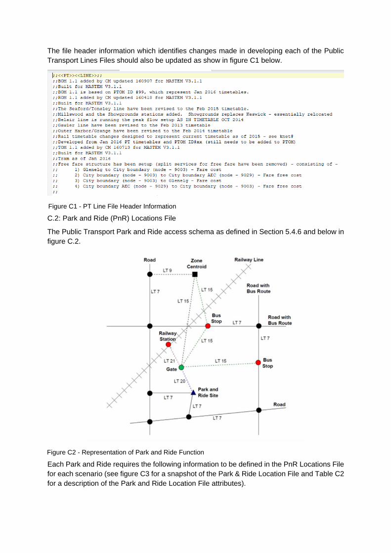
The file header information which identifies changes made in developing each of the Public
Transport Lines Files should also be updated as show in figure C1 below.
C.2: Park and Ride (PnR) Locations File
The Public Transport Park and Ride access schema as defined in Section 5.4.6 and below in
figure C.2.
Each Park and Ride requires the following information to be defined in the PnR Locations File
for each scenario (see figure C3 for a snapshot of the Park & Ride Location File and Table C2
for a description of the Park and Ride Location File attributes).
Figure C1 - PT Line File Header Information
Figure C2 - Representation of Park and Ride Function
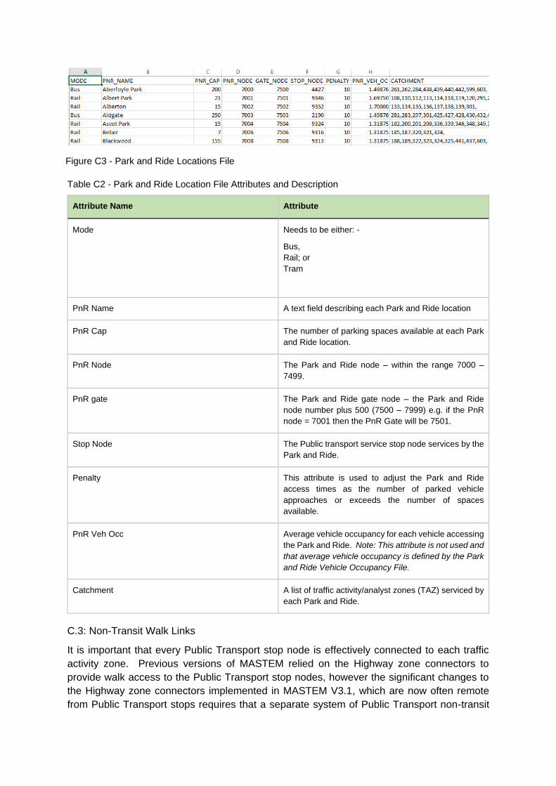
Attribute Name Attribute
Mode Needs to be either: -
Bus,
Rail; or
Tram
PnR Name A text field describing each Park and Ride location
PnR Cap The number of parking spaces available at each Park
and Ride location.
PnR Node The Park and Ride node – within the range 7000 –
7499.
PnR gate The Park and Ride gate node – the Park and Ride
node number plus 500 (7500 – 7999) e.g. if the PnR
node = 7001 then the PnR Gate will be 7501.
Stop Node The Public transport service stop node services by the
Park and Ride.
Penalty This attribute is used to adjust the Park and Ride
access times as the number of parked vehicle
approaches or exceeds the number of spaces
available.
PnR Veh Occ Average vehicle occupancy for each vehicle accessing
the Park and Ride. Note: This attribute is not used and
that average vehicle occupancy is defined by the Park
and Ride Vehicle Occupancy File.
Catchment A list of traffic activity/analyst zones (TAZ) serviced by
each Park and Ride.
C.3: Non-Transit Walk Links
It is important that every Public Transport stop node is effectively connected to each traffic
activity zone. Previous versions of MASTEM relied on the Highway zone connectors to
provide walk access to the Public Transport stop nodes, however the significant changes to
the Highway zone connectors implemented in MASTEM V3.1, which are now often remote
from Public Transport stops requires that a separate system of Public Transport non-transit
Figure C3 - Park and Ride Locations File
Table C2 - Park and Ride Location File Attributes and Description
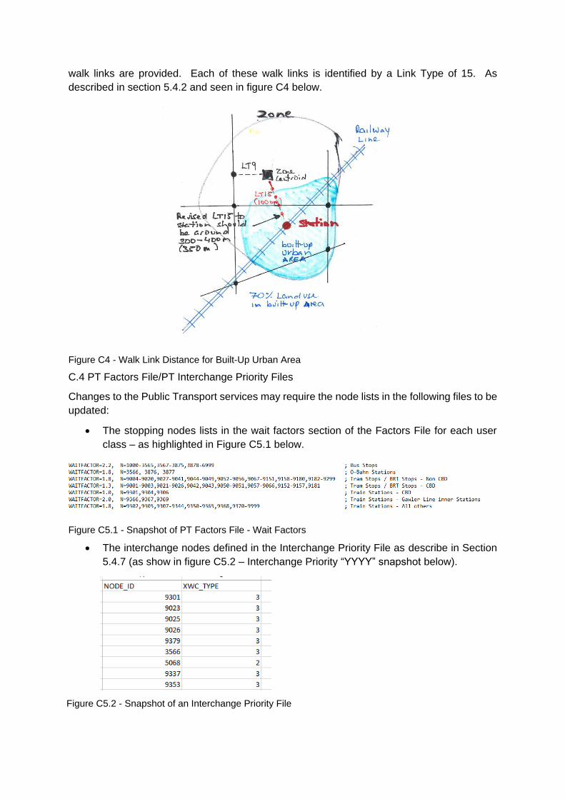
walk links are provided. Each of these walk links is identified by a Link Type of 15. As
described in section 5.4.2 and seen in figure C4 below.
C.4 PT Factors File/PT Interchange Priority Files
Changes to the Public Transport services may require the node lists in the following files to be
updated:
The stopping nodes lists in the wait factors section of the Factors File for each user
class – as highlighted in Figure C5.1 below.
The interchange nodes defined in the Interchange Priority File as describe in Section
5.4.7 (as show in figure C5.2 – Interchange Priority “YYYY” snapshot below).
Figure C4 - Walk Link Distance for Built-Up Urban Area
Figure C5.1 - Snapshot of PT Factors File - Wait Factors
Figure C5.2 - Snapshot of an Interchange Priority File

Appendix D – Highway Input Files Updating

D.1: Highway Junction Files
The junction model within MASTEM should closely emulate SCATS performance, although
this will be limited to some extent by the limitations of the CUBE junction modelling. The
junction model should also be robust under a range of possible scenarios / time periods in
order to minimise the effort required to effectively develop this critical component of the model.
The Highway Junction Files for each time period for each scenario run follow standard Cube
practice however some attributes need to be carefully and consistently defined as noted
below:
Time Period Variation:
To the extent possible, attribute values should be the same for all time periods, and should be
chosen such that intersection performance is acceptable across all time periods. Separate
time period files should only be used when banned movements or lane use changes
throughout the day.
Signal Operation:
In general all signalised intersections / junctions should be coded using the Adaptive Signal,
Geometric (HCM) option.
Lane Geometry:
The lane geometry should match the existing / proposed layouts.
Phases:
Signal phasing should match either the existing arrangement or – for proposed new signals –
the preferred arrangement for four way intersections which provides greatest flexibility is to
adopt leading and trailing right turn movements as shown in Figure D1.1.
Figure D1.1 - Leading Trailing Right Turn Movement Diagram

For T junctions, the three phase signal operation is the preferred design of signals for input
into the future year MASTEM Model as shown in Figure D1.2.
For all new locations all right turns should be controlled (no right turn filters).
Cycle times should be 120 seconds for all time periods unless the intersection operates with
longer cycle times across all time periods. Phase times for existing signalised intersections
should be based on operational data, and the range between the minimum and maximum
phase times should cover the likely range for all time periods.
D.2 Turn Penalty Files
Turn penalty files may be used to ban movements or to add delay to specific movements.
Figure D1.2 - Single T Junction Three Phase Diagram

Appendix E - MASTEM User Benefit Calculation Tool
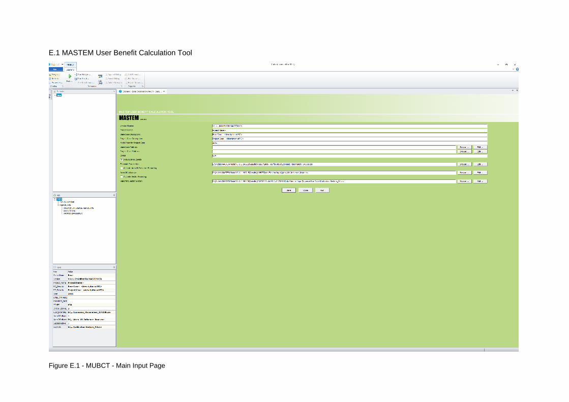
E.1 MASTEM User Benefit Calculation Tool
Figure E.1 - MUBCT - Main Input Page
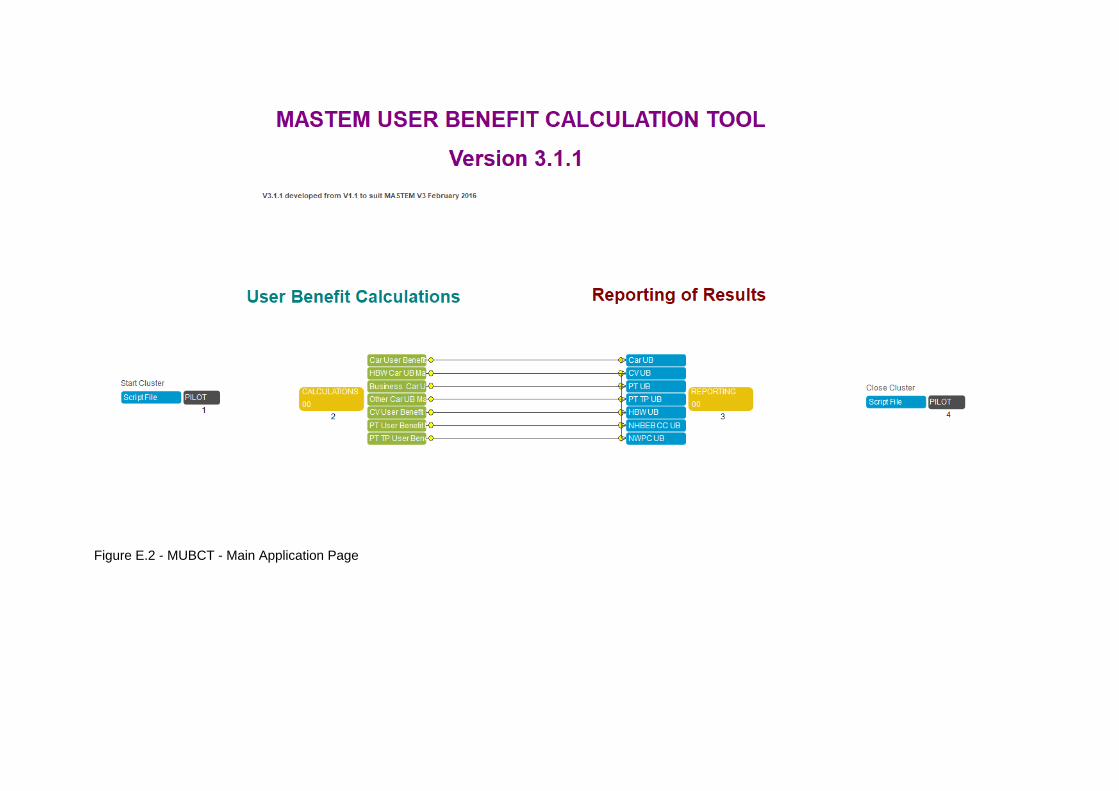
Figure E.2 - MUBCT - Main Application Page
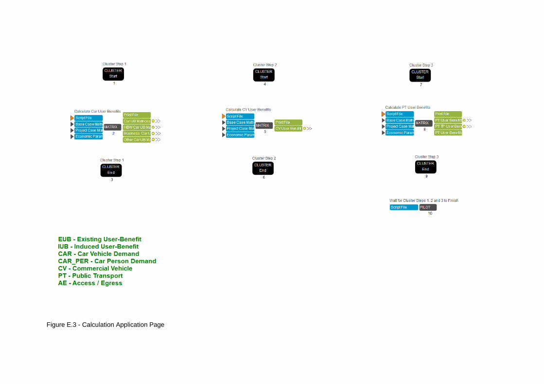
Figure E.3 - Calculation Application Page
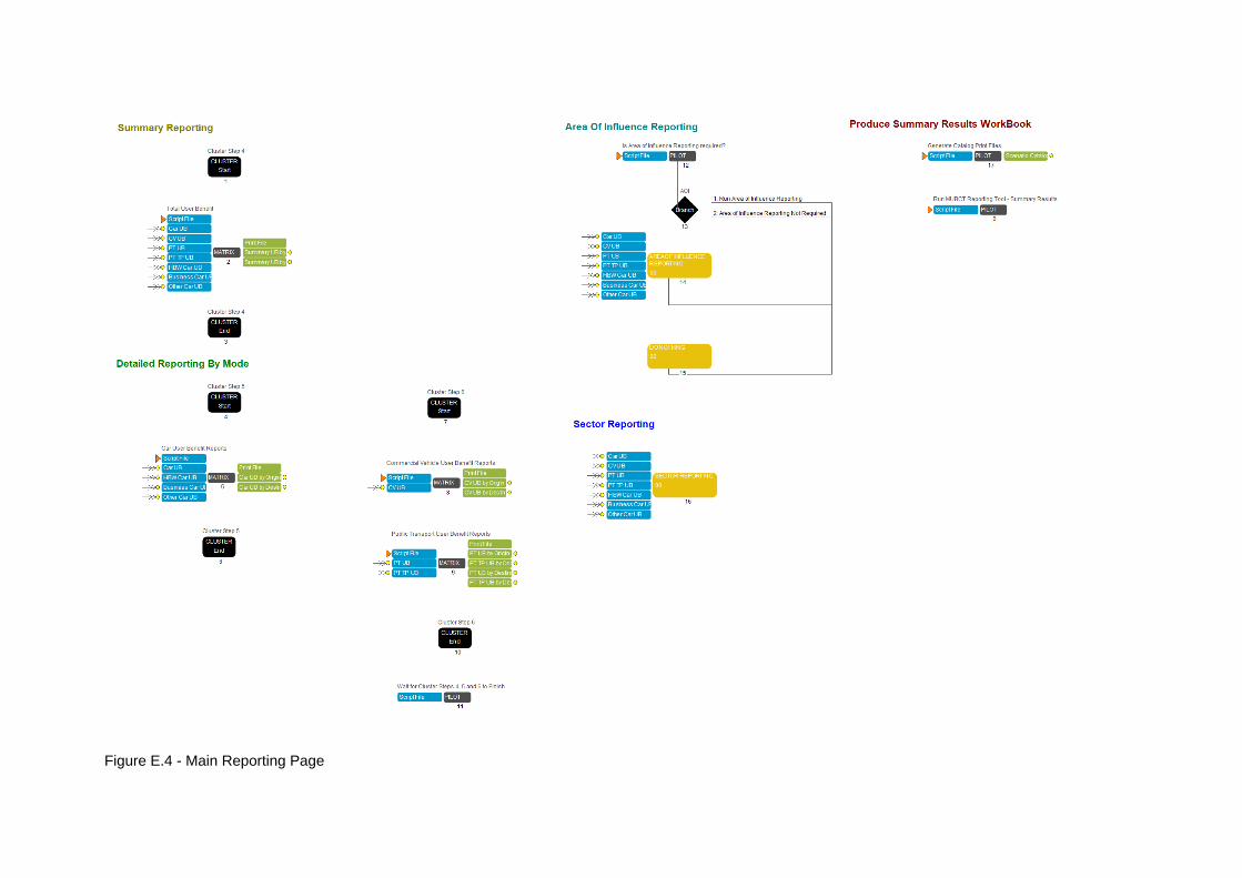
Figure E.4 - Main Reporting Page
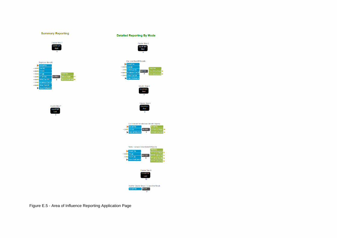
Figure E.5 - Area of Influence Reporting Application Page
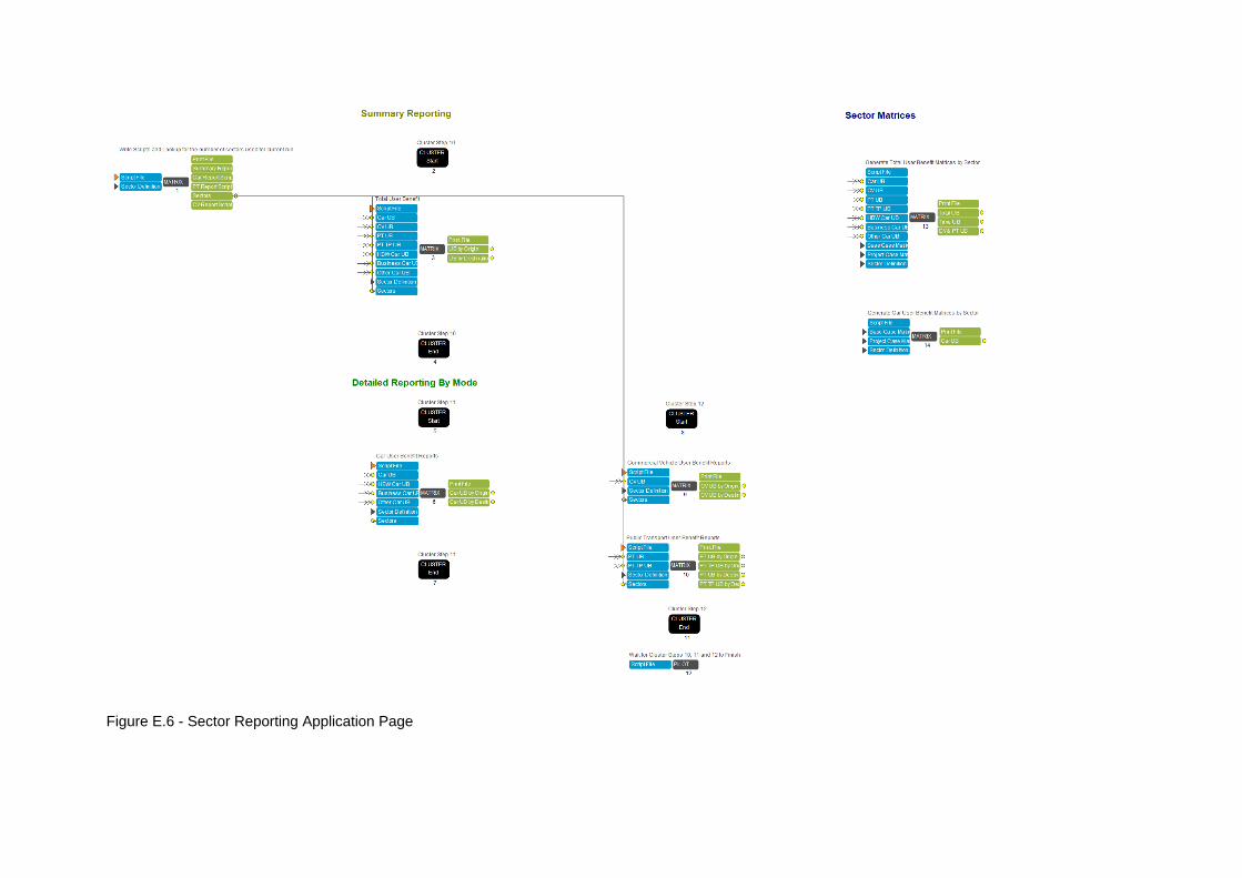
Figure E.6 - Sector Reporting Application Page

E.2 Origin-Destination User Benefit Tool (ODUBT)
Origin-Destination User Benefit Tool (ODUBT)
Technical Report
For: Department of Planning, Transport and Infrastrcutrue
3rd August 2015
Project Name: ODUBT
Project Number: 3005444
Report for: Department of Planning, Transport and Infrastructure
PREPARATION, REVIEW AND AUTHORISATION
Revision # Date Prepared by Reviewed by Approved for Issue by
1 03/08/15 J Parrott P. Tisato J Parrott
ISSUE REGISTER
Distribution List Date Issued Number of Copies
Department of Planning, Transport and Infrastructure: 03/08/15 Electronic
SMEC staff: 03/08/15 Electronic
Associates: N/A
SMEC COMPANY DETAILS
SMEC AUSTRALIA
Level 4, 19 Grenfell Street, Adelaide, SA 5000
Tel: 08 8225 9800
Fax: 08 8225 9850
Email: [email protected]
www.smec.com
The information within this document is and shall remain the property Department of Planning, Transport and Infrastructure (DPTI)
Origin-Destination User Benefit Tool Technical Report | Revision No. 1 | 3 August 2015 Page | i
TABLE OF CONTENTS
1 INTRODUCTION ................................................................................................................. 1
2 USER BENEFIT CALCULATIONS ..................................................................................... 2
2.1 User Benefit Formula ....................................................................................................... 2
2.2 Mode Notation ................................................................................................................. 3
2.3 Generalised Cost ............................................................................................................. 3
2.4 Parameter Values ............................................................................................................ 6
3 REPORTING ....................................................................................................................... 8
4 HOW ODUBT OPERATES ............................................................................................... 10
4.1 Methodology .................................................................................................................. 10
4.2 Input Files and Catalogue Key ...................................................................................... 11
4.3 Structure of Tool ............................................................................................................ 14
4.4 Location of ODUBT Folders/Files within the MASTEM Suite ........................................ 14
4.5 Output Files ................................................................................................................... 15
APPENDIX A FURTHER DETAILS RELATED TO MASTEM ........................................... 23
A.1 Derivation of Outputs from MASTEM V2.3.0 ................................................................. 23
A.2 MASTEM V3 .................................................................................................................. 25
ODUBT Technical Report | Revision No. 1 | 3 August 2015 Page | 1
1 INTRODUCTION
This is the Technical Report for version 2.0 of the DPTI1 Origin-Destination User Benefit Tool (ODUBT). Version 1.0 of the tool and its associated report were developed by SKM. Version 2.0 has been produced by SMEC for DPTI.
ODUBT is a tool for calculating the user-benefits associated urban transport infrastructure projects on an origin-destination basis. The methodology is recommended by Infrastructure Australia as best practice for the assessment of large urban transport initiatives.
For a given transport initiative, the ODUBT specifically calculates user benefits on a disaggregated basis for each origin-destination pair. It then aggregates across all origin-destination pairs to give the total user-benefit for the initiative. ODUBT uses as its primary input results from DPTI’s strategic travel demand model MASTEM.
ODUBT standard results are currently produced by:
Mode of travel (private car home-based work trip, private car non-work trip, commercial/business car, commercial vehicles (CV, i.e. truck) and public transport
Time period AM peak, PM peak and Off-Peak (OP) time periods
For the Adelaide metropolitan area as a whole (as modelled by MASTEM), and on an Area of Influence basis (optional).
The tool was developed in the CUBE Voyager and Microsoft Excel software platforms. User-benefit calculations are not required after every run of MASTEM, thus the ODUBT was developed as a separate post-processing tool that forms part of the MASTEM suite. The tool resides in the MASTEM ‘Results’ folder along with the summary statistics reporting. To provide consistency with the summary statistics reporting, the results from the ODUBT were developed with a similar style including a catalogue key report, specific to the ODUBT catalogue key.
This current version of ODUBT operates using the following software:
MASTEM V2.3.0 (21/08/10) which includes the Summary Statistics 2 update;
CUBE Voyager 6.1.0 (SP1) and Microsoft Excel 2010.
All parameter values have been provided by DPTI.
The rest of this technical report documents:
the formula and parameters used for user benefit calculations (Section 2);
the reporting provided by the tool (Section 3);
how the ODUBT operates (Section 4); and
1 Department of Planning, Transport and Infrastructure
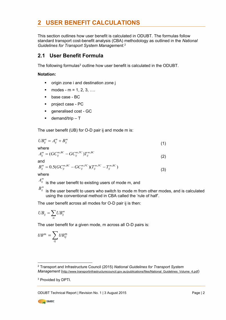
ODUBT Technical Report | Revision No. 1 | 3 August 2015 Page | 2
2 USER BENEFIT CALCULATIONS
This section outlines how user benefit is calculated in ODUBT. The formulas follow standard transport cost-benefit analysis (CBA) methodology as outlined in the National Guidelines for Transport System Management.2
2.1 User Benefit Formula
The following formulas3 outline how user benefit is calculated in the ODUBT.
Notation:
origin zone i and destination zone j
modes - m = 1, 2, 3, ….
base case - BC
project case - PC
generalised cost - GC
demand/trip – T
The user benefit (UB) for O-D pair ij and mode m is:
m
ij
m
ij
m
ij BAUB (1)
where BCm
ij
PCm
ij
BCm
ij
m
ij TGCGCA,,, )(
(2) and
))((5.0 ,,,, BCm
ij
PCm
ij
PCm
ij
BCm
ij
m
ij TTGCGCB (3)
where m
ijA is the user benefit to existing users of mode m, and m
ijB is the user benefit to users who switch to mode m from other modes, and is calculated using the conventional method in CBA called the ‘rule of half’.
The user benefit across all modes for O-D pair ij is then:
m
m
ijij UBUB
The user benefit for a given mode, m across all O-D pairs is: ��� = ���
2 Transport and Infrastructure Council (2015) National Guidelines for Transport System Management (http://www.transportinfrastructurecouncil.gov.au/publications/files/National_Guidelines_Volume_4.pdf)
3 Provided by DPTI.
ODUBT Technical Report | Revision No. 1 | 3 August 2015 Page | 3
The total user benefit for the initiative can be calculated by summing across either all O-D pairs or all modes: �� = �� = ����
ODUBT currently calculates user benefits on the basis of ‘perceived’ user costs. A separate ‘resource correction’, to adjust for difference between perceived and resource costs, is currently calculated outside ODUBT using aggregate outputs from the MASTEM model. In due course, the resource correction calculations could also be undertaken within ODUBT.
2.2 Mode Notation
The following notation is used for the four modes modelled:
PV CAR: private car – private, non-business travel by car
COMM CAR: commercial car – non-private business travel by car
CV: truck, referred to here (as per MASTEM) as ‘commercial vehicle’
PT: public transport (bus, train and tram)
2.3 Generalised Cost
Each mode has its own generalised cost equation which takes into account all cost
elements incurred by the user. The equations are listed below:
GCPV CAR=(VoTPV CAR/60) x TimeCAR + (VOCPV CAR)*DistanceCAR + P x IP
GCCOM CAR=(VoTCOMM CAR/60) x TimeCAR + (VOCCOM CAR)*DistanceCAR + P x IP
GCCV=(VoTCV/60) x TimeCV + (VOCCV)*DistanceCV
GCPT=F x IF + (VoTPT/60) x (TAE x WAE + TPKR x WPKR + TW x WW + TI BUS x WI BUS + TI TRAM x WI TRAM
+ TI TRAIN x WI TRAIN + TTP x WP + TTAT x WAT + TTWT x WWT)
where for any trip between an origin-destination (O-D) pair:
VoTPV CAR is the value of time in dollars per person-hour for private car trips
VoTCOMM CAR is the value of time in dollars per person-hour for commercial car trips
VoTCV is the value of time in dollars per vehicle-hour for CV trips
VoTPT is the value of time in dollars per person-hour for PT trips
VOCPV CAR is the vehicle operating cost in dollars per vehicle-kilometre for private car
trips
VOCCOMM CAR is the vehicle operating cost in dollars per vehicle-kilometre for commercial
car trips – at this point in time, the same value is used as for VOCPV CAR
VOCCV is the vehicle operating cost in dollars per vehicle-kilometre for CV trips
ODUBT Technical Report | Revision No. 1 | 3 August 2015 Page | 4
TimeCAR is the highway skim for average car travel time
TimeCV is the highway skim for average CV travel time
DistanceCAR is the highway skim for average car travel distance
DistanceCV is the highway skim for average CV travel distance
P is the weighted average parking charge that car vehicles pay per trip
IP is the indexation factor for parking charges
F is the weighted average fare that public transport passengers pay per trip
IF is the indexation factor for Public Transport Fares
TAE is the time cost for walk access/egress
WAE is the weighting for walk access/egress
TPKR is the time cost for park/kiss and ride
WPKR is the weighting for park/kiss and ride
TW is the waiting time for the initial boarding
WW is the weighting on the waiting time for the initial boarding
TI BUS is the time cost for bus in vehicle travel time
WI BUS is the weighting for bus in vehicle travel time
TI TRAM is the time cost for tram in vehicle travel time
WI TRAM is the weighting for tram in vehicle travel time
TI TRAIN is the time cost for train in vehicle travel time
WI TRAIN is the weighting for train in vehicle travel time
TTP is the total transfer penalty
WP is the weighting for time costs for transfers
TTAT is the total access/walk time for service transfers
WAT is the weighting for access/walk times for transfers
TTWT is the total time waiting for service transfers
WWT is the weighting for wait times for transfers
Notes:
1) Generalised cost is calculated for each O-D pair, resulting in an O-D matrix of
generalised cost (referred to as ‘skims’).
2) Time is calculated in minutes.
3) PV CAR represents both home-based work (HBW) and Non-Work car trips. COMM CAR
combines non-home based employer’s business (NHBEB) car trips and commercial
car trips. HBW and NHBEB are trip purpose codes from the MASTEM model.
ODUBT Technical Report | Revision No. 1 | 3 August 2015 Page | 5
4) The GCPT formula is the application of the formula in the ATC (2006)4 within the scope
of the MASTEM model. The variations in application here are as follows:
a) Park/kiss and ride costs are shown separately from other access/egress costs
b) In-vehicle time costs are shown for each of the three public transport modes (bus,
train and tram) because a trip can consist of several boardings of different public
transport modes
c) IP and IF allow the dollar values built into the MASTEM model to be indexed up to
current value
d) TTP is equivalent to NT * TP in Transport and Infrastructure Council (2015). TTP is
the way MASTEM reports.
e) TTAT is equivalent to NT * TAT in Transport and Infrastructure Council (2015). TTAT
is the way MASTEM reports.
f) TTWT is equivalent to NT * TWT in Transport and Infrastructure Council (2015). TTWT
is the way MASTEM reports.
4 Australian Transport Council (2006), National Guidelines for Transport System Management. Vol.4, p.45. Can be referenced via the weblink in footnote 2 – at the website, go to > About > Reference Documents
ODUBT Technical Report | Revision No. 1 | 3 August 2015 Page | 6
2.4 Parameter Values
User benefits are calculated using parameter values supplied by DPTI. The values at June 2015 are listed in Table 1.
Table 1 Parameter Values
Parameter Value Unit
VOTPV CAR CAR_VoT 15.40 $'s_per_person_per_hour
VOTCOMM CAR Comm_CAR_VoT 46.70 $'s_per_person_per_hour
VOTCV CV_VoT (1) 47.90 $'s_per_vehicle_per_hour
VOCCAR CAR_VOC 0.27 $'s_per_vehicle_per_kilometre
VOTCV CV_VOC 0.72 $'s_per_vehicle_per_kilometre
VOTPT PT_VoT 15.40 $'s_per_person_per_hour
P Car_Parking_Charge (2),(3) $’s per trip
F PT_Fare (2),(4) $’s per trip
IP Car_parking_charge_indexation_factor 1.0
IF PT_fare_indexation_factor 1.16
WAE Walk_Access_Time_Weighting 1.4 Multiplier of time
WPKR Park_and_Ride_Access_Time_Weighting 1 Multiplier of time
WW Wait_Time_Initial_Boarding_Weighting 1.4 Multiplier of time
WIBUS Bus_In-Vehicle_Time_Weighting 1 Multiplier of time
WITRAIN Train_In-Vehicle_Time_Weighting 1 Multiplier of time
WITRAM Tram_In-Vehicle_Time_Weighting 1 Multiplier of time
WP Transfer_Penalty_Weighting 1.4 Minutes
WAT Walk_Transfer_Time_Weighting 1 Multiplier of time
WWT Wait_Time_Transfer_Boarding_Weighting 1.2 Multiplier of time
Car_Annualisation_Factor 328 Multiplier of traffic volume
CV_Annualisation_Factor 286 Multiplier of traffic volume
PT_Annualisation_Factor 280 Multiplier of patronage
Notes:
(1) Varies with the mix of heavy trucks. Hence needs to be specified for each project assessment. The figure reported here represents traffic mix on South Road at Mile End (between Henley Beach Road and Sir Donald Bradman Drive).
(2) Parking (P) and fare (F) costs are built into the MASTEM model.5
(3) Calculated in MASTEM on an O-D basis and by trip type. Values in MASTEM range from $5.55 to $9.05 for work based trips i.e. all day parking and range from $0.90 to $2.05 for non-work trips i.e. short term parking. These numbers are in 2006 dollars. DPTI does not have a parking cost index series, and is not aware of one in ABS series. The motoring cost sub-group of the ABS CPI series (6401, Table 11) shows a small decline in real terms (relative to general inflation [ABS, CPI series, 6401.0, Adelaide, All Groups] from 2006 to 2015. In the absence of better information, the indexation factor Ip was kept at 1.0.
5 See 2014 DPTI report #83244222 MASTEM Travel Demand Model – Methodology and Assumptions.
ODUBT Technical Report | Revision No. 1 | 3 August 2015 Page | 7
(4) Calculated in MASTEM on a trip purpose basis using the Adelaide Metro fare structure and fare levels. In MASTEM the fare data is in 2006 dollars, and are then indexed up in real terms to 2015 dollars via the indexation factor IF. IF was calculated based on real fare indexation by combining the fare data with general inflation data (ABC, CPI series, 6401.0, Adelaide, All Groups).
Sources:
VoT and VOC: Austroads (2012) Guide to Project Evaluation, Part 4 – values supplied by DPTI
PT weightings: Australian Transport Council (2006), National Guidelines for Transport System Management, Vol 4, appendix A (see footnote 4 for weblink).
Annualisation factors: supplied by DPTI
Car Parking Charge indexation factor: supplied by DPTI, see note 3 above
PT Fare indexation factors: Supplied by DPTI, based on internal DPTI data, see note 4 above.
ODUBT Technical Report | Revision No. 1 | 3 August 2015 Page | 8
3 REPORTING
The outputs from ODUBT relate to the four dimensions of calculations undertaken in the tool. They are:
1) Mode – Private Car Person, Commercial Car Person, Commercial Vehicle and Public Transport Passenger6
2) Cost Component – Car and CV: Time and Distance
Public Transport: Fare, Walk Access/Egress and Transfer, Park
and Ride Access/Egress, Bus/Train/Tram In-Vehicle Time, Initial
and Transfer Wait Times and Transfer Penalties
3) Time Period - AM, OP and PM
4) User Type – Existing and Induced7
The calculations are performed and available at the O-D level; however it is not practical to report the results at this level (320x3208 matrices). Thus outputs are produced at several geographical levels. They are as follows:
whole of Adelaide metropolitan area as modelled by MASTEM;
at the origin zone level;
at the destination zone level; and
by area of influence (AOI).
The purpose of the AOI option is to remove the influence of traffic effects in parts of the transport network where one would expect the project to have little impact. This removes the potential influence of any MASTEM ‘model noise’ in those locations. All travel demand models contain ‘model noise’, and this is a practical method for limiting its influence in user benefit calculations.
The AOI option works by zeroing out results for all O-D pairs where both the origin zone and destination zone are not included within the specified AOI zone list. If one or both of the origin zone and destination zone are included in the AOI zone list, the result for the OD pair is still included in the user benefit results.
Table 2, Table 3, Table 4 and Table 5 below detail the outputs (denoted by an X). All outputs generated are at the origin and destination level respectively. For consistency and efficiency, results produced at the origin and destination level are also generated for the sector and area of influence reporting as well.
6 Due to the coarse nature of the Walk and Cycle networks within MASTEM, both non-motorised
modes are not included in the calculations.
7 ‘Existing’ refers to the level of use in the base case, and ‘induced’ refers to the change in use between the base case and project case. The project case has both existing and induced use.
8 Although MASTEM V2.3 does not have 320 zones, the highest zone number is 320. For reporting purposes, it is easier to include non-active zones so that the results are consecutive from zone 1 through to zone 320. Non-Active zones are greyed out in the report to denote they are inactive.
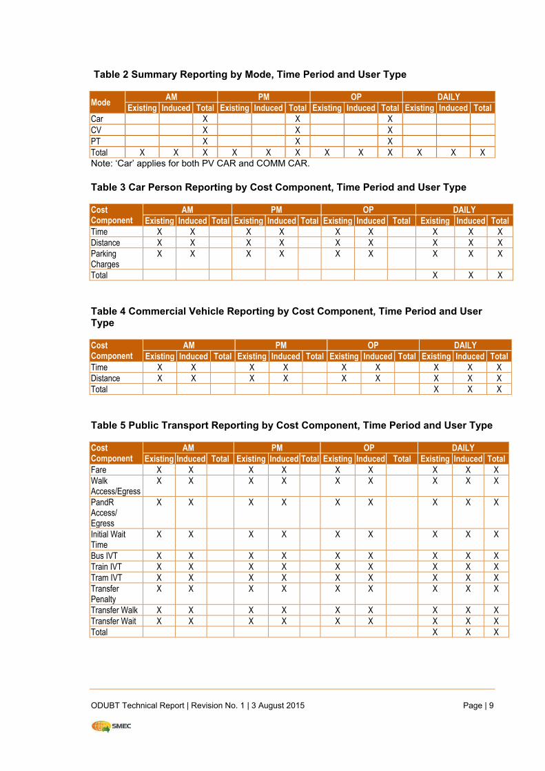
ODUBT Technical Report | Revision No. 1 | 3 August 2015 Page | 9
Table 2 Summary Reporting by Mode, Time Period and User Type
Mode AM PM OP DAILY
Existing Induced Total Existing Induced Total Existing Induced Total Existing Induced Total
Car X X X CV X X X PT X X X Total X X X X X X X X X X X X Note: ‘Car’ applies for both PV CAR and COMM CAR.
Table 3 Car Person Reporting by Cost Component, Time Period and User Type
Cost Component
AM PM OP DAILY
Existing Induced Total Existing Induced Total Existing Induced Total Existing Induced Total
Time X X X X X X X X X Distance X X X X X X X X X Parking Charges
X X X X X X X X X
Total X X X
Table 4 Commercial Vehicle Reporting by Cost Component, Time Period and User Type
Cost Component
AM PM OP DAILY
Existing Induced Total Existing Induced Total Existing Induced Total Existing Induced Total
Time X X X X X X X X X Distance X X X X X X X X X Total X X X
Table 5 Public Transport Reporting by Cost Component, Time Period and User Type
Cost Component
AM PM OP DAILY
Existing Induced Total Existing Induced Total Existing Induced Total Existing Induced Total
Fare X X X X X X X X X Walk Access/Egress
X X X X X X X X X
PandR Access/ Egress
X X X X X X X X X
Initial Wait Time
X X X X X X X X X
Bus IVT X X X X X X X X X Train IVT X X X X X X X X X Tram IVT X X X X X X X X X Transfer Penalty
X X X X X X X X X
Transfer Walk X X X X X X X X X Transfer Wait X X X X X X X X X Total X X X
ODUBT Technical Report | Revision No. 1 | 3 August 2015 Page | 10
4 HOW ODUBT OPERATES
4.1 Methodology
MASTEM V2.3 provides results by car (person/vehicle), public transport, bicycle, walk and commercial vehicle. Results for walk and bicycle are not included in the ODUBT at this point in time.
Calculations are performed by mode (private car person/ commercial car person/ commercial vehicle [truck]/ public transport passenger) by time period (AM, PM and Off-Peak) by origin-destination zone (~320x320) with all results converted to dollar values.
The MASTEM model is a series of mathematical equations and parameter values used to model travel demand in Adelaide. The equations are estimated using Adelaide data. ‘Cube Voyager’ is a software package specifically designed to develop and run strategic transport models, and has been used to develop and run MASTEM.
MASTEM has developed using Cube Voyager, and, to provide consistency between the ODUBT and MASTEM, the ODUBT has also been developed in CUBE Voyager. All matrix calculations are undertaken using the CUBE Voyager software and summary results are then provided in Microsoft Excel to ensure end users are able to access results without requiring specialised software.
The steps to create a report that details the total User-Benefit for a given set of MASTEM base and project case runs are as follows:
1. MASTEM is run twice (1 base case and 1 project case run).
2. Parameter value input files are updated as required.
3. (Optional) – Area of Influence input files are created or updated as required.
4. A new scenario is set up using the ODUBT in CUBE with all input files linked
correctly in the catalogue key. A ‘scenario’ is a specific pair of base and project case runs from MASTEM.
5. ODUBT is run for the given scenario.
6. The excel report sheet is automatically created and closed during the CUBE run.
7. The excel report sheet is located in the respective scenarios output folder i.e. for
scenario TEST it is located in: C:\MASTEM Model\Results\ODUBT\Base\TEST.
A flow diagram of the overall process is provided in Figure 1.
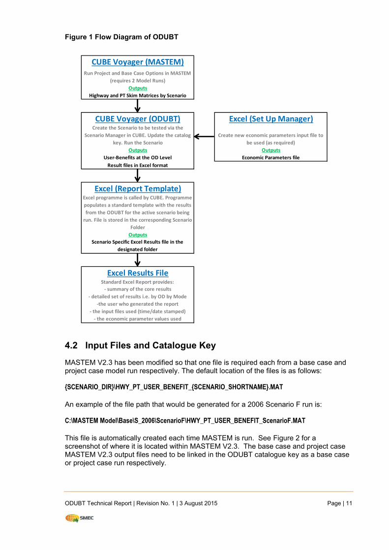
ODUBT Technical Report | Revision No. 1 | 3 August 2015 Page | 11
Figure 1 Flow Diagram of ODUBT
4.2 Input Files and Catalogue Key
MASTEM V2.3 has been modified so that one file is required each from a base case and project case model run respectively. The default location of the files is as follows:
{SCENARIO_DIR}\HWY_PT_USER_BENEFIT_{SCENARIO_SHORTNAME}.MAT
An example of the file path that would be generated for a 2006 Scenario F run is:
C:\MASTEM Model\Base\S_2006\ScenarioF\HWY_PT_USER_BENEFIT_ScenarioF.MAT
This file is automatically created each time MASTEM is run. See Figure 2 for a screenshot of where it is located within MASTEM V2.3. The base case and project case MASTEM V2.3 output files need to be linked in the ODUBT catalogue key as a base case or project case run respectively.
CUBE Voyager (MASTEM)
Run Project and Base Case Options in MASTEM
(requires 2 Model Runs)
Outputs
Highway and PT Skim Matrices by Scenario
CUBE Voyager (ODUBT) Excel (Set Up Manager)Create the Scenario to be tested via the
Scenario Manager in CUBE. Update the catalog
key. Run the Scenario
Create new economic parameters input file to
be used (as required)
Outputs Outputs
User-Benefits at the OD Level Economic Parameters file
Result files in Excel format
Excel (Report Template)Excel programme is called by CUBE. Programme
populates a standard template with the results
from the ODUBT for the active scenario being
run. File is stored in the corresponding Scenario
Folder
Outputs
Scenario Specific Excel Results file in the
designated folder
Excel Results FileStandard Excel Report provides:
- summary of the core results
- detailed set of results i.e. by OD by Mode
-the user who generated the report
- the input files used (time/date stamped)
- the economic parameter values used
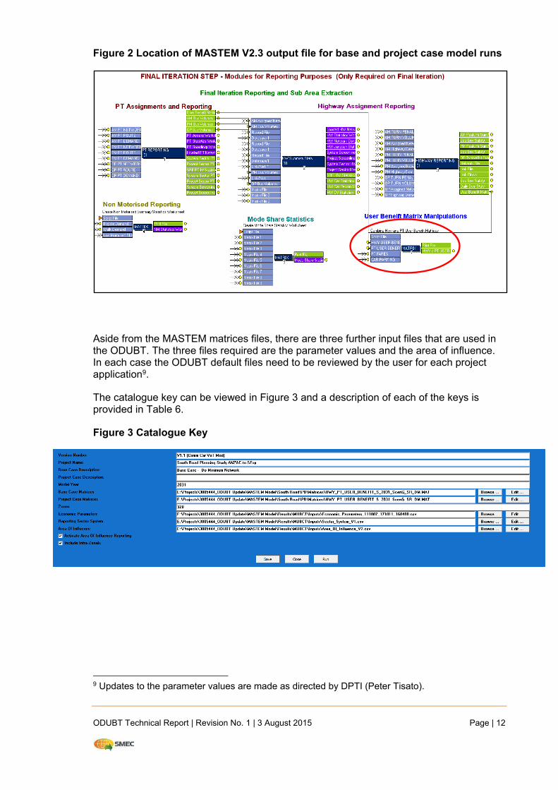
ODUBT Technical Report | Revision No. 1 | 3 August 2015 Page | 12
Figure 2 Location of MASTEM V2.3 output file for base and project case model runs
Aside from the MASTEM matrices files, there are three further input files that are used in the ODUBT. The three files required are the parameter values and the area of influence. In each case the ODUBT default files need to be reviewed by the user for each project application9.
The catalogue key can be viewed in Figure 3 and a description of each of the keys is provided in Table 6.
Figure 3 Catalogue Key
9 Updates to the parameter values are made as directed by DPTI (Peter Tisato).
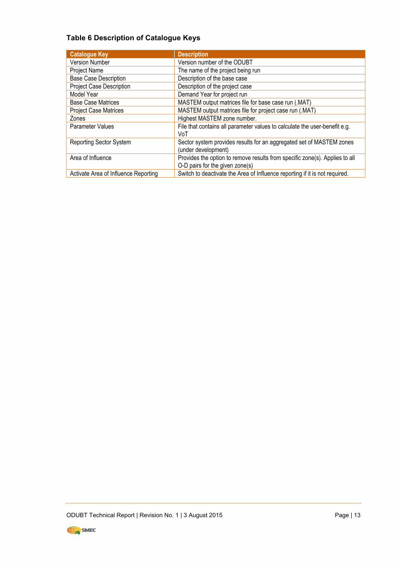
ODUBT Technical Report | Revision No. 1 | 3 August 2015 Page | 13
Table 6 Description of Catalogue Keys
Catalogue Key Description
Version Number Version number of the ODUBT Project Name The name of the project being run Base Case Description Description of the base case Project Case Description Description of the project case Model Year Demand Year for project run Base Case Matrices MASTEM output matrices file for base case run (.MAT) Project Case Matrices MASTEM output matrices file for project case run (.MAT) Zones Highest MASTEM zone number. Parameter Values File that contains all parameter values to calculate the user-benefit e.g.
VoT Reporting Sector System Sector system provides results for an aggregated set of MASTEM zones
(under development) Area of Influence Provides the option to remove results from specific zone(s). Applies to all
O-D pairs for the given zone(s) Activate Area of Influence Reporting Switch to deactivate the Area of Influence reporting if it is not required.
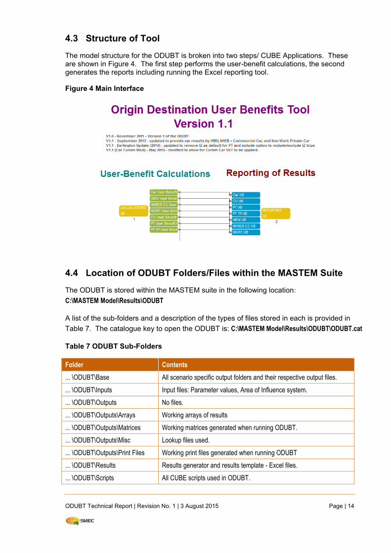
ODUBT Technical Report | Revision No. 1 | 3 August 2015 Page | 14
4.3 Structure of Tool
The model structure for the ODUBT is broken into two steps/ CUBE Applications. These are shown in Figure 4. The first step performs the user-benefit calculations, the second generates the reports including running the Excel reporting tool.
Figure 4 Main Interface
4.4 Location of ODUBT Folders/Files within the MASTEM Suite
The ODUBT is stored within the MASTEM suite in the following location:
C:\MASTEM Model\Results\ODUBT
A list of the sub-folders and a description of the types of files stored in each is provided in
Table 7. The catalogue key to open the ODUBT is: C:\MASTEM Model\Results\ODUBT\ODUBT.cat
Table 7 ODUBT Sub-Folders
Folder Contents
... \ODUBT\Base All scenario specific output folders and their respective output files.
... \ODUBT\Inputs Input files: Parameter values, Area of Influence system.
... \ODUBT\Outputs No files.
... \ODUBT\Outputs\Arrays Working arrays of results
... \ODUBT\Outputs\Matrices Working matrices generated when running ODUBT.
... \ODUBT\Outputs\Misc Lookup files used.
... \ODUBT\Outputs\Print Files Working print files generated when running ODUBT
... \ODUBT\Results Results generator and results template - Excel files.
... \ODUBT\Scripts All CUBE scripts used in ODUBT.
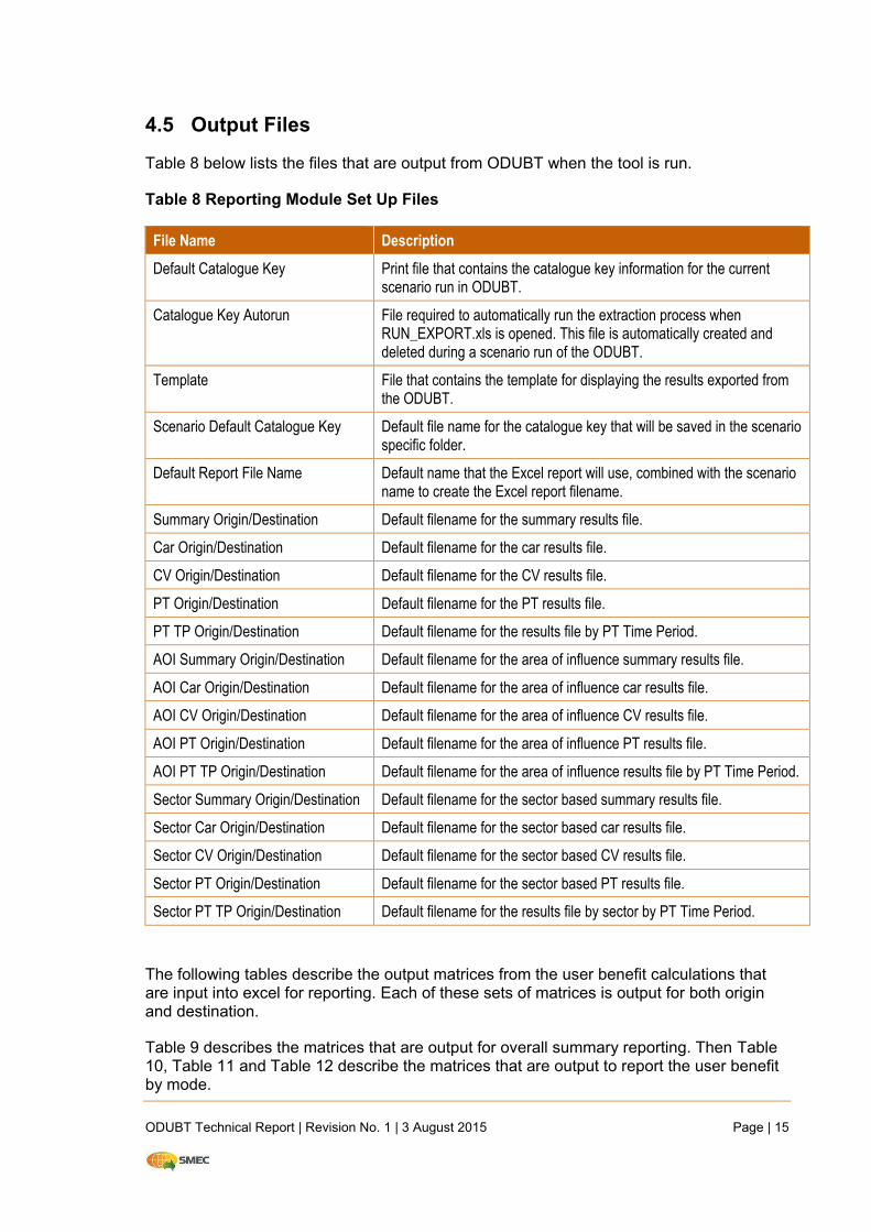
ODUBT Technical Report | Revision No. 1 | 3 August 2015 Page | 15
4.5 Output Files
Table 8 below lists the files that are output from ODUBT when the tool is run.
Table 8 Reporting Module Set Up Files
File Name Description
Default Catalogue Key Print file that contains the catalogue key information for the current scenario run in ODUBT.
Catalogue Key Autorun File required to automatically run the extraction process when RUN_EXPORT.xls is opened. This file is automatically created and deleted during a scenario run of the ODUBT.
Template File that contains the template for displaying the results exported from the ODUBT.
Scenario Default Catalogue Key Default file name for the catalogue key that will be saved in the scenario specific folder.
Default Report File Name Default name that the Excel report will use, combined with the scenario name to create the Excel report filename.
Summary Origin/Destination Default filename for the summary results file.
Car Origin/Destination Default filename for the car results file.
CV Origin/Destination Default filename for the CV results file.
PT Origin/Destination Default filename for the PT results file.
PT TP Origin/Destination Default filename for the results file by PT Time Period.
AOI Summary Origin/Destination Default filename for the area of influence summary results file.
AOI Car Origin/Destination Default filename for the area of influence car results file.
AOI CV Origin/Destination Default filename for the area of influence CV results file.
AOI PT Origin/Destination Default filename for the area of influence PT results file.
AOI PT TP Origin/Destination Default filename for the area of influence results file by PT Time Period.
Sector Summary Origin/Destination Default filename for the sector based summary results file.
Sector Car Origin/Destination Default filename for the sector based car results file.
Sector CV Origin/Destination Default filename for the sector based CV results file.
Sector PT Origin/Destination Default filename for the sector based PT results file.
Sector PT TP Origin/Destination Default filename for the results file by sector by PT Time Period.
The following tables describe the output matrices from the user benefit calculations that are input into excel for reporting. Each of these sets of matrices is output for both origin and destination.
Table 9 describes the matrices that are output for overall summary reporting. Then Table 10, Table 11 and Table 12 describe the matrices that are output to report the user benefit by mode.
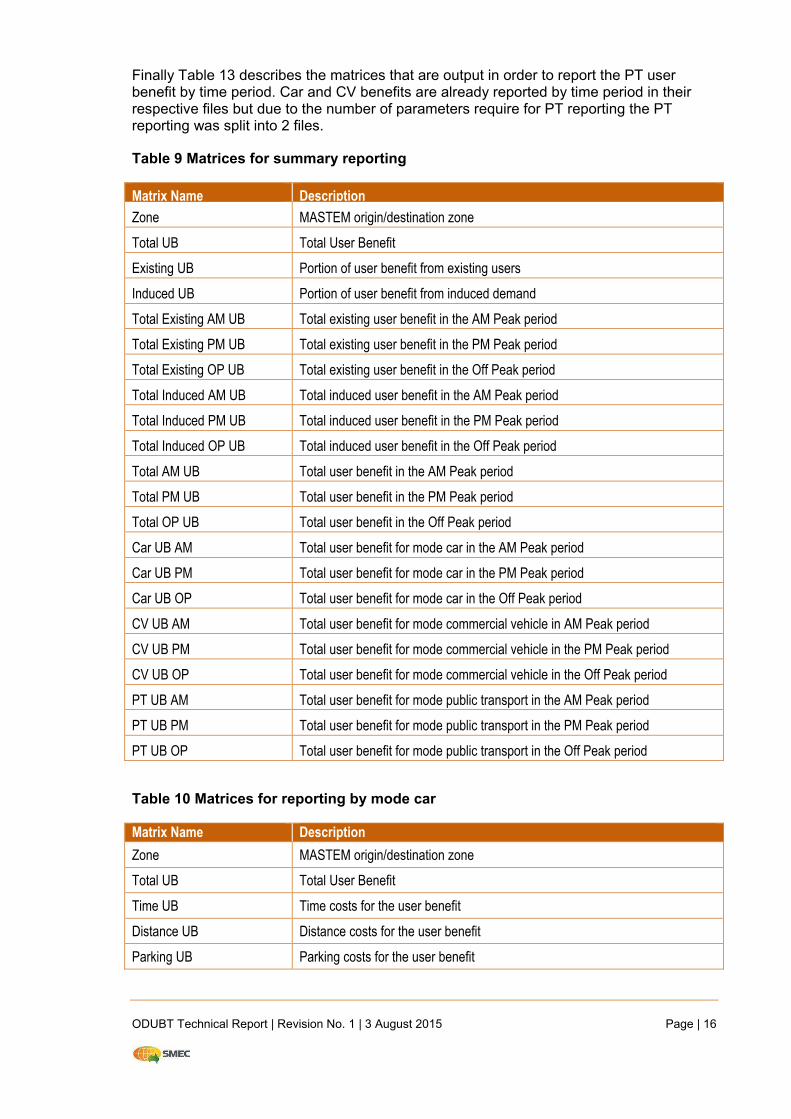
ODUBT Technical Report | Revision No. 1 | 3 August 2015 Page | 16
Finally Table 13 describes the matrices that are output in order to report the PT user benefit by time period. Car and CV benefits are already reported by time period in their respective files but due to the number of parameters require for PT reporting the PT reporting was split into 2 files.
Table 9 Matrices for summary reporting
Matrix Name Description
Zone MASTEM origin/destination zone
Total UB Total User Benefit
Existing UB Portion of user benefit from existing users
Induced UB Portion of user benefit from induced demand
Total Existing AM UB Total existing user benefit in the AM Peak period
Total Existing PM UB Total existing user benefit in the PM Peak period
Total Existing OP UB Total existing user benefit in the Off Peak period
Total Induced AM UB Total induced user benefit in the AM Peak period
Total Induced PM UB Total induced user benefit in the PM Peak period
Total Induced OP UB Total induced user benefit in the Off Peak period
Total AM UB Total user benefit in the AM Peak period
Total PM UB Total user benefit in the PM Peak period
Total OP UB Total user benefit in the Off Peak period
Car UB AM Total user benefit for mode car in the AM Peak period
Car UB PM Total user benefit for mode car in the PM Peak period
Car UB OP Total user benefit for mode car in the Off Peak period
CV UB AM Total user benefit for mode commercial vehicle in AM Peak period
CV UB PM Total user benefit for mode commercial vehicle in the PM Peak period
CV UB OP Total user benefit for mode commercial vehicle in the Off Peak period
PT UB AM Total user benefit for mode public transport in the AM Peak period
PT UB PM Total user benefit for mode public transport in the PM Peak period
PT UB OP Total user benefit for mode public transport in the Off Peak period
Table 10 Matrices for reporting by mode car
Matrix Name Description
Zone MASTEM origin/destination zone
Total UB Total User Benefit
Time UB Time costs for the user benefit
Distance UB Distance costs for the user benefit
Parking UB Parking costs for the user benefit
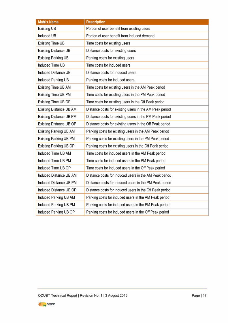
ODUBT Technical Report | Revision No. 1 | 3 August 2015 Page | 17
Matrix Name Description
Existing UB Portion of user benefit from existing users
Induced UB Portion of user benefit from induced demand
Existing Time UB Time costs for existing users
Existing Distance UB Distance costs for existing users
Existing Parking UB Parking costs for existing users
Induced Time UB Time costs for induced users
Induced Distance UB Distance costs for induced users
Induced Parking UB Parking costs for induced users
Existing Time UB AM Time costs for existing users in the AM Peak period
Existing Time UB PM Time costs for existing users in the PM Peak period
Existing Time UB OP Time costs for existing users in the Off Peak period
Existing Distance UB AM Distance costs for existing users in the AM Peak period
Existing Distance UB PM Distance costs for existing users in the PM Peak period
Existing Distance UB OP Distance costs for existing users in the Off Peak period
Existing Parking UB AM Parking costs for existing users in the AM Peak period
Existing Parking UB PM Parking costs for existing users in the PM Peak period
Existing Parking UB OP Parking costs for existing users in the Off Peak period
Induced Time UB AM Time costs for induced users in the AM Peak period
Induced Time UB PM Time costs for induced users in the PM Peak period
Induced Time UB OP Time costs for induced users in the Off Peak period
Induced Distance UB AM Distance costs for induced users in the AM Peak period
Induced Distance UB PM Distance costs for induced users in the PM Peak period
Induced Distance UB OP Distance costs for induced users in the Off Peak period
Induced Parking UB AM Parking costs for induced users in the AM Peak period
Induced Parking UB PM Parking costs for induced users in the PM Peak period
Induced Parking UB OP Parking costs for induced users in the Off Peak period
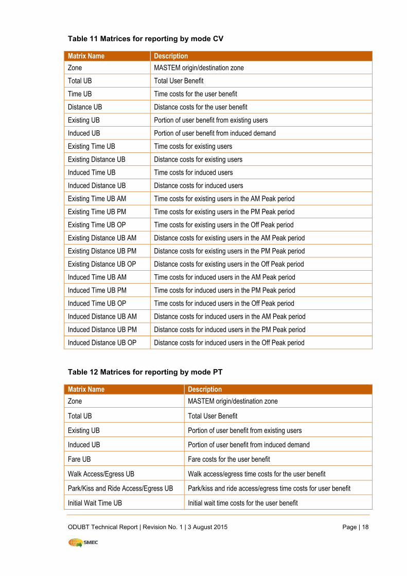
ODUBT Technical Report | Revision No. 1 | 3 August 2015 Page | 18
Table 11 Matrices for reporting by mode CV
Matrix Name Description
Zone MASTEM origin/destination zone
Total UB Total User Benefit
Time UB Time costs for the user benefit
Distance UB Distance costs for the user benefit
Existing UB Portion of user benefit from existing users
Induced UB Portion of user benefit from induced demand
Existing Time UB Time costs for existing users
Existing Distance UB Distance costs for existing users
Induced Time UB Time costs for induced users
Induced Distance UB Distance costs for induced users
Existing Time UB AM Time costs for existing users in the AM Peak period
Existing Time UB PM Time costs for existing users in the PM Peak period
Existing Time UB OP Time costs for existing users in the Off Peak period
Existing Distance UB AM Distance costs for existing users in the AM Peak period
Existing Distance UB PM Distance costs for existing users in the PM Peak period
Existing Distance UB OP Distance costs for existing users in the Off Peak period
Induced Time UB AM Time costs for induced users in the AM Peak period
Induced Time UB PM Time costs for induced users in the PM Peak period
Induced Time UB OP Time costs for induced users in the Off Peak period
Induced Distance UB AM Distance costs for induced users in the AM Peak period
Induced Distance UB PM Distance costs for induced users in the PM Peak period
Induced Distance UB OP Distance costs for induced users in the Off Peak period
Table 12 Matrices for reporting by mode PT
Matrix Name Description
Zone MASTEM origin/destination zone
Total UB Total User Benefit
Existing UB Portion of user benefit from existing users
Induced UB Portion of user benefit from induced demand
Fare UB Fare costs for the user benefit
Walk Access/Egress UB Walk access/egress time costs for the user benefit
Park/Kiss and Ride Access/Egress UB Park/kiss and ride access/egress time costs for user benefit
Initial Wait Time UB Initial wait time costs for the user benefit

ODUBT Technical Report | Revision No. 1 | 3 August 2015 Page | 19
Matrix Name Description
Bus In-Vehicle Time UB Bus in vehicle time costs for the user benefit
Train In-Vehicle Time UB Train in vehicle time costs for the user benefit
Tram In-Vehicle Time UB Tram in vehicle time costs for the user benefit
Transfer Penalty UB Transfer penalty costs for the user benefit
Transfer Walk Time UB Transfer walk time costs for the user benefit
Transfer Wait Time UB Transfer wait time costs for the user benefit
Existing Fare UB Fare costs for existing users
Existing Walk Access/Egress UB Walk access/egress time costs for existing users
Existing Park/Kiss and Ride Access/Egress UB Park/kiss and ride access/egress time costs for existing users
Existing Initial Wait Time UB Initial wait time costs for existing users
Existing Bus In-Vehicle Time UB Bus in vehicle time costs for existing users
Existing Train In-Vehicle Time UB Train in vehicle time costs for existing users
Existing Tram In-Vehicle Time UB Tram in vehicle time costs for existing users
Existing Transfer Penalty UB Transfer penalty costs for existing users
Existing Transfer Walk Time UB Transfer walk time costs for existing users
Existing Transfer Wait Time UB Transfer wait time costs for existing users
Induced Fare UB Fare costs for induced users
Induced Walk Access/Egress UB Walk access/egress time costs for induced users
Induced Park/Kiss and Ride Access/Egress UB Park/kiss and ride access/egress time costs for induced users
Induced Initial Wait Time UB Initial wait time costs for induced users
Induced Bus In-Vehicle Time UB Bus in vehicle time costs for induced users
Induced Train In-Vehicle Time UB Train in vehicle time costs for induced users
Induced Tram In-Vehicle Time UB Tram in vehicle time costs for induced users
Induced Transfer Penalty UB Transfer penalty costs for induced users
Induced Transfer Walk Time UB Transfer walk time costs for induced users
Induced Transfer Wait Time UB Transfer wait time costs for induced users
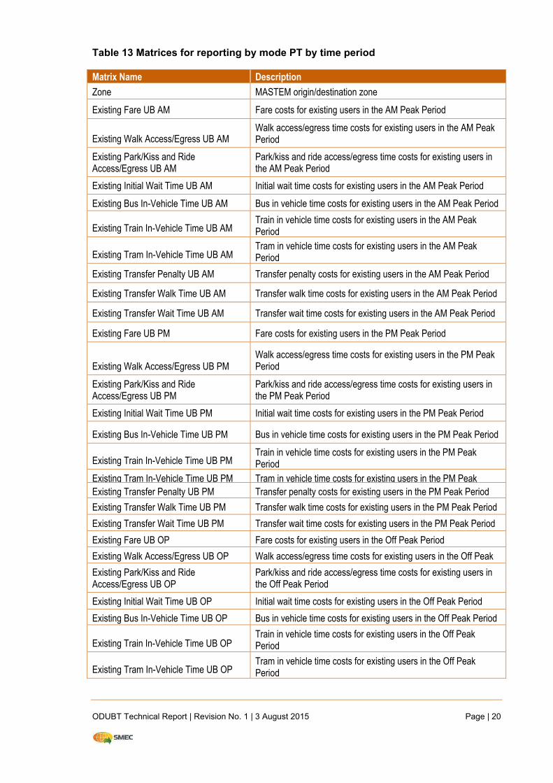
ODUBT Technical Report | Revision No. 1 | 3 August 2015 Page | 20
Table 13 Matrices for reporting by mode PT by time period
Matrix Name Description
Zone MASTEM origin/destination zone
Existing Fare UB AM Fare costs for existing users in the AM Peak Period
Existing Walk Access/Egress UB AM Walk access/egress time costs for existing users in the AM Peak Period
Existing Park/Kiss and Ride Access/Egress UB AM
Park/kiss and ride access/egress time costs for existing users in the AM Peak Period
Existing Initial Wait Time UB AM Initial wait time costs for existing users in the AM Peak Period
Existing Bus In-Vehicle Time UB AM Bus in vehicle time costs for existing users in the AM Peak Period
Existing Train In-Vehicle Time UB AM Train in vehicle time costs for existing users in the AM Peak Period
Existing Tram In-Vehicle Time UB AM Tram in vehicle time costs for existing users in the AM Peak Period
Existing Transfer Penalty UB AM Transfer penalty costs for existing users in the AM Peak Period
Existing Transfer Walk Time UB AM Transfer walk time costs for existing users in the AM Peak Period
Existing Transfer Wait Time UB AM Transfer wait time costs for existing users in the AM Peak Period
Existing Fare UB PM Fare costs for existing users in the PM Peak Period
Existing Walk Access/Egress UB PM Walk access/egress time costs for existing users in the PM Peak Period
Existing Park/Kiss and Ride Access/Egress UB PM
Park/kiss and ride access/egress time costs for existing users in the PM Peak Period
Existing Initial Wait Time UB PM Initial wait time costs for existing users in the PM Peak Period
Existing Bus In-Vehicle Time UB PM Bus in vehicle time costs for existing users in the PM Peak Period
Existing Train In-Vehicle Time UB PM Train in vehicle time costs for existing users in the PM Peak Period
Existing Tram In-Vehicle Time UB PM Tram in vehicle time costs for existing users in the PM Peak
Existing Transfer Penalty UB PM Transfer penalty costs for existing users in the PM Peak Period
Existing Transfer Walk Time UB PM Transfer walk time costs for existing users in the PM Peak Period
Existing Transfer Wait Time UB PM Transfer wait time costs for existing users in the PM Peak Period
Existing Fare UB OP Fare costs for existing users in the Off Peak Period
Existing Walk Access/Egress UB OP Walk access/egress time costs for existing users in the Off Peak Period Existing Park/Kiss and Ride
Access/Egress UB OP Park/kiss and ride access/egress time costs for existing users in the Off Peak Period
Existing Initial Wait Time UB OP Initial wait time costs for existing users in the Off Peak Period
Existing Bus In-Vehicle Time UB OP Bus in vehicle time costs for existing users in the Off Peak Period
Existing Train In-Vehicle Time UB OP Train in vehicle time costs for existing users in the Off Peak Period
Existing Tram In-Vehicle Time UB OP Tram in vehicle time costs for existing users in the Off Peak Period
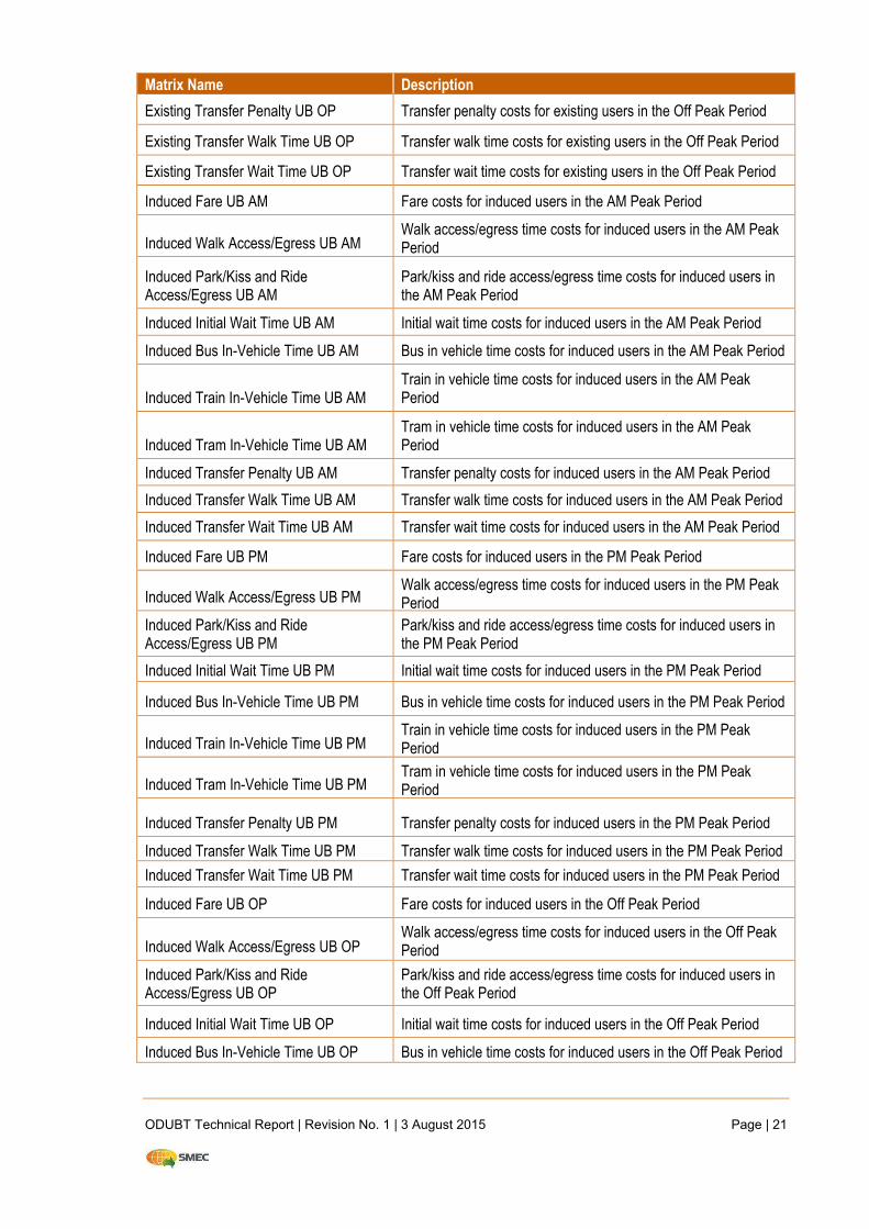
ODUBT Technical Report | Revision No. 1 | 3 August 2015 Page | 21
Matrix Name Description
Existing Transfer Penalty UB OP Transfer penalty costs for existing users in the Off Peak Period
Existing Transfer Walk Time UB OP Transfer walk time costs for existing users in the Off Peak Period
Existing Transfer Wait Time UB OP Transfer wait time costs for existing users in the Off Peak Period
Induced Fare UB AM Fare costs for induced users in the AM Peak Period
Induced Walk Access/Egress UB AM Walk access/egress time costs for induced users in the AM Peak Period
Induced Park/Kiss and Ride Access/Egress UB AM
Park/kiss and ride access/egress time costs for induced users in the AM Peak Period
Induced Initial Wait Time UB AM Initial wait time costs for induced users in the AM Peak Period
Induced Bus In-Vehicle Time UB AM Bus in vehicle time costs for induced users in the AM Peak Period
Induced Train In-Vehicle Time UB AM Train in vehicle time costs for induced users in the AM Peak Period
Induced Tram In-Vehicle Time UB AM Tram in vehicle time costs for induced users in the AM Peak Period
Induced Transfer Penalty UB AM Transfer penalty costs for induced users in the AM Peak Period
Induced Transfer Walk Time UB AM Transfer walk time costs for induced users in the AM Peak Period
Induced Transfer Wait Time UB AM Transfer wait time costs for induced users in the AM Peak Period
Induced Fare UB PM Fare costs for induced users in the PM Peak Period
Induced Walk Access/Egress UB PM Walk access/egress time costs for induced users in the PM Peak Period
Induced Park/Kiss and Ride Access/Egress UB PM
Park/kiss and ride access/egress time costs for induced users in the PM Peak Period
Induced Initial Wait Time UB PM Initial wait time costs for induced users in the PM Peak Period
Induced Bus In-Vehicle Time UB PM Bus in vehicle time costs for induced users in the PM Peak Period
Induced Train In-Vehicle Time UB PM Train in vehicle time costs for induced users in the PM Peak Period
Induced Tram In-Vehicle Time UB PM Tram in vehicle time costs for induced users in the PM Peak Period
Induced Transfer Penalty UB PM Transfer penalty costs for induced users in the PM Peak Period
Induced Transfer Walk Time UB PM Transfer walk time costs for induced users in the PM Peak Period
Induced Transfer Wait Time UB PM Transfer wait time costs for induced users in the PM Peak Period
Induced Fare UB OP Fare costs for induced users in the Off Peak Period
Induced Walk Access/Egress UB OP Walk access/egress time costs for induced users in the Off Peak Period
Induced Park/Kiss and Ride Access/Egress UB OP
Park/kiss and ride access/egress time costs for induced users in the Off Peak Period
Induced Initial Wait Time UB OP Initial wait time costs for induced users in the Off Peak Period
Induced Bus In-Vehicle Time UB OP Bus in vehicle time costs for induced users in the Off Peak Period
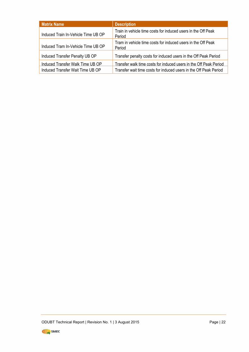
ODUBT Technical Report | Revision No. 1 | 3 August 2015 Page | 22
Matrix Name Description
Induced Train In-Vehicle Time UB OP Train in vehicle time costs for induced users in the Off Peak Period
Induced Tram In-Vehicle Time UB OP Tram in vehicle time costs for induced users in the Off Peak Period
Induced Transfer Penalty UB OP Transfer penalty costs for induced users in the Off Peak Period
Induced Transfer Walk Time UB OP Transfer walk time costs for induced users in the Off Peak Period
Induced Transfer Wait Time UB OP Transfer wait time costs for induced users in the Off Peak Period
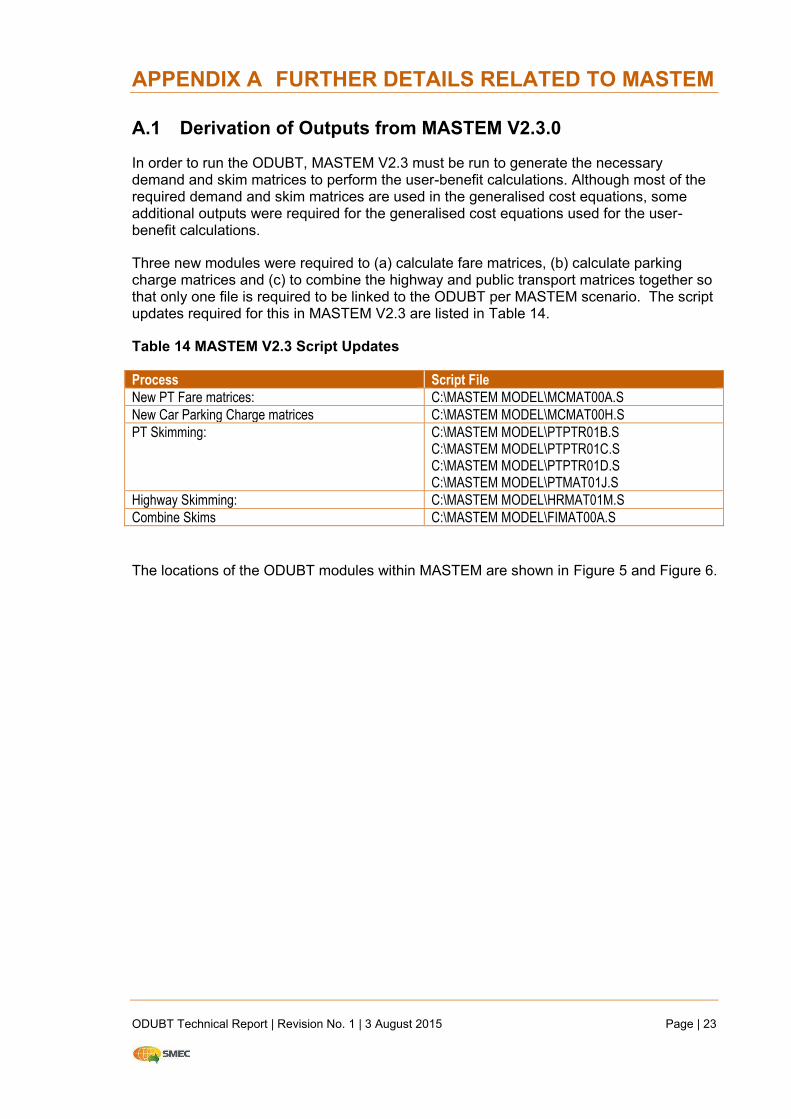
ODUBT Technical Report | Revision No. 1 | 3 August 2015 Page | 23
APPENDIX A FURTHER DETAILS RELATED TO MASTEM
A.1 Derivation of Outputs from MASTEM V2.3.0
In order to run the ODUBT, MASTEM V2.3 must be run to generate the necessary demand and skim matrices to perform the user-benefit calculations. Although most of the required demand and skim matrices are used in the generalised cost equations, some additional outputs were required for the generalised cost equations used for the user-benefit calculations.
Three new modules were required to (a) calculate fare matrices, (b) calculate parking charge matrices and (c) to combine the highway and public transport matrices together so that only one file is required to be linked to the ODUBT per MASTEM scenario. The script updates required for this in MASTEM V2.3 are listed in Table 14.
Table 14 MASTEM V2.3 Script Updates
Process Script File
New PT Fare matrices: C:\MASTEM MODEL\MCMAT00A.S New Car Parking Charge matrices C:\MASTEM MODEL\MCMAT00H.S PT Skimming: C:\MASTEM MODEL\PTPTR01B.S
C:\MASTEM MODEL\PTPTR01C.S C:\MASTEM MODEL\PTPTR01D.S C:\MASTEM MODEL\PTMAT01J.S
Highway Skimming: C:\MASTEM MODEL\HRMAT01M.S Combine Skims C:\MASTEM MODEL\FIMAT00A.S
The locations of the ODUBT modules within MASTEM are shown in Figure 5 and Figure 6.
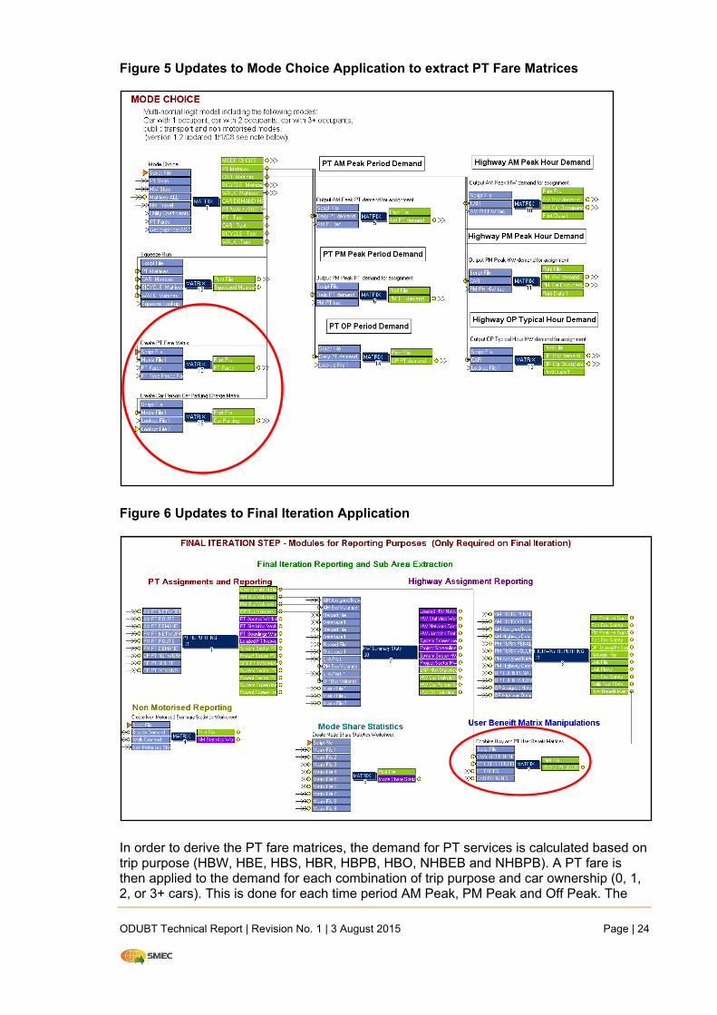
ODUBT Technical Report | Revision No. 1 | 3 August 2015 Page | 24
Figure 5 Updates to Mode Choice Application to extract PT Fare Matrices
Figure 6 Updates to Final Iteration Application
In order to derive the PT fare matrices, the demand for PT services is calculated based on trip purpose (HBW, HBE, HBS, HBR, HBPB, HBO, NHBEB and NHBPB). A PT fare is then applied to the demand for each combination of trip purpose and car ownership (0, 1, 2, or 3+ cars). This is done for each time period AM Peak, PM Peak and Off Peak. The
ODUBT Technical Report | Revision No. 1 | 3 August 2015 Page | 25
average PT fare is then calculated as the total PT fares divided by the total PT demand for each time period.
To derive the parking charge matrices, the parking is divided up into parking for HBW, parking for other home based trip purposes, parking for NHBEB and parking for NHBPB. The parking matrices are then adjusted based on a percentage of car vehicle trips that do not pay for parking in the CBD. The demand for parking is calculated based on car vehicle trips and trip purpose, with the relevant parking charge then applied to each trip purpose. The average parking charge is then calculated as the total parking charges divided by the total parking demand for each time period.
To derive the PT mode access transfers the total trips and total PT boardings parameters are used. The total PT boardings is calculated as the sum of the average number of bus boardings, average number of train boardings and average number of tram boardings. It is assumed there are no transfers for intra-zonal trips, otherwise for each trip the number of transfers is the number of boardings less 1 to account for the initial boarding for the trip (unless the average number of boardings is less than 1, in which case it is assumed there are no transfers). When calculating the transfer wait time and transfer walk time, the actual times rather than perceived times are used.
A.2 MASTEM V3
The ODUBT currently operates in MASTEM V2.3 only. The production of an equivalent version of ODUBT for MASTEM V3 should simply require transfer to the MASTEM V3 platform. A thorough review will be needed to confirm updates required as MASTEM V3 performs some calculations in slightly different formats to V2.3 and this will need to be assessed carefully. The ODUBT will also need to be updated to be compatible with MASTEM V3 due to the additional time period being modelled in MASTEM V3.

Appendix F – MASTEM Audit Check List
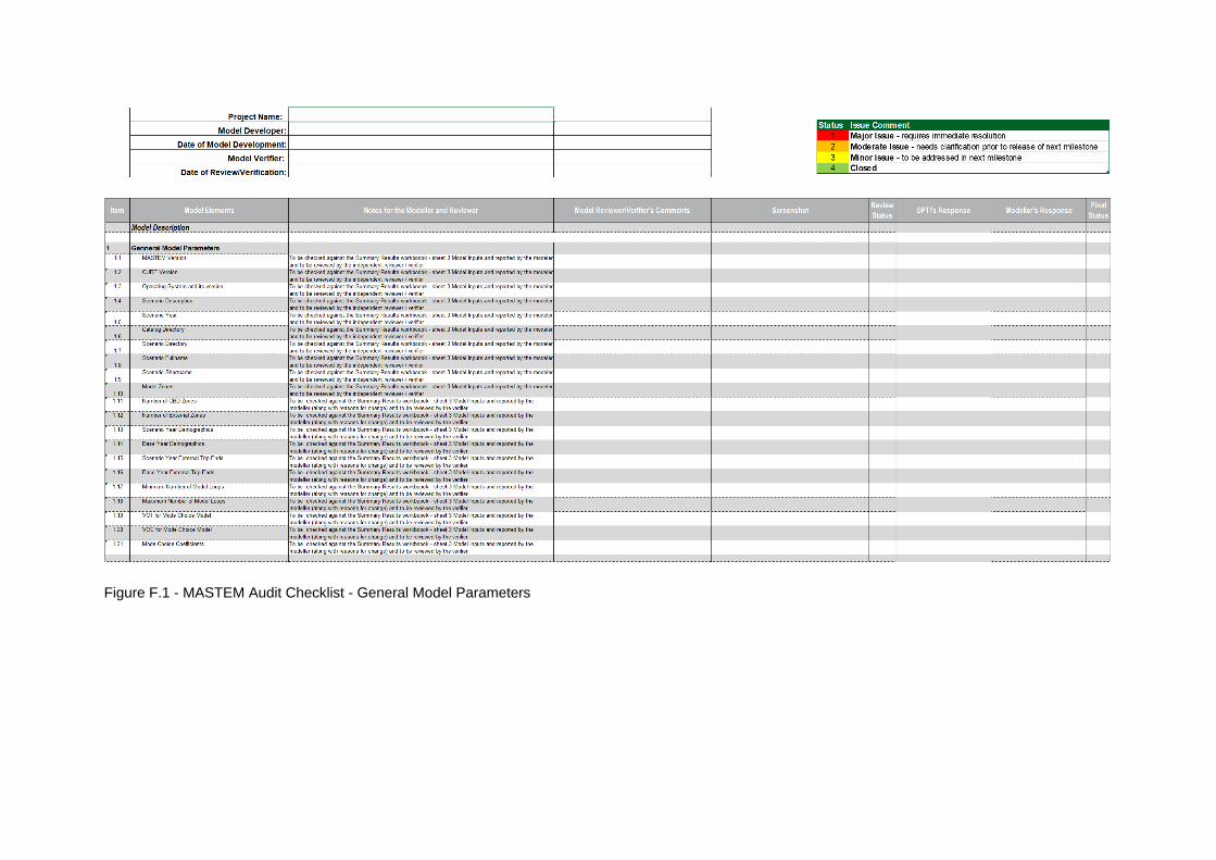
Figure F.1 - MASTEM Audit Checklist - General Model Parameters
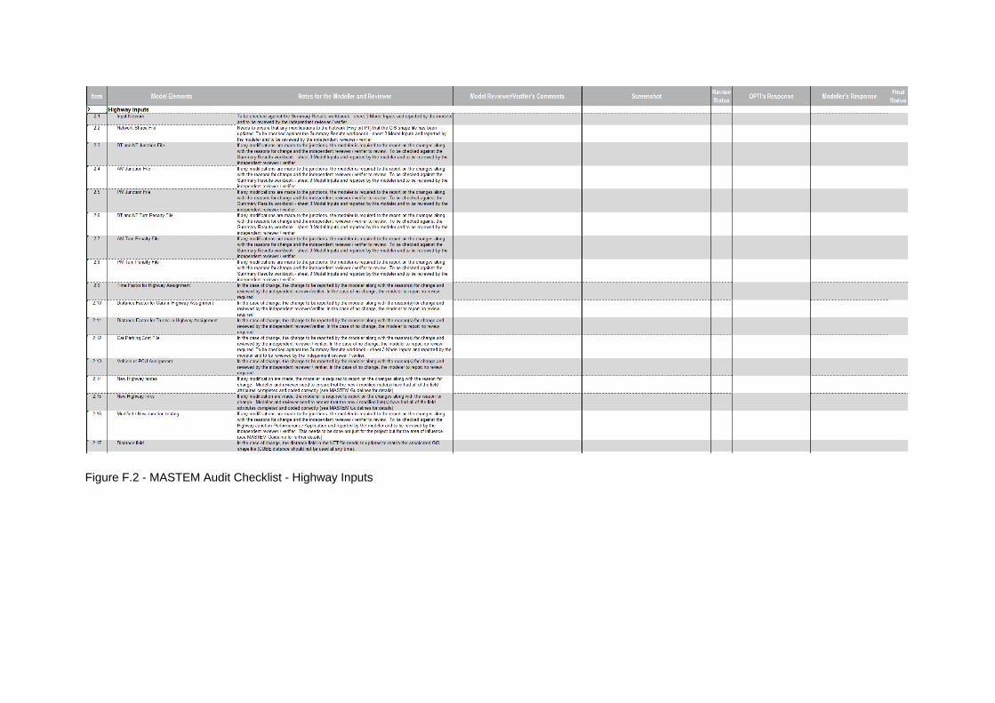
Figure F.2 - MASTEM Audit Checklist - Highway Inputs
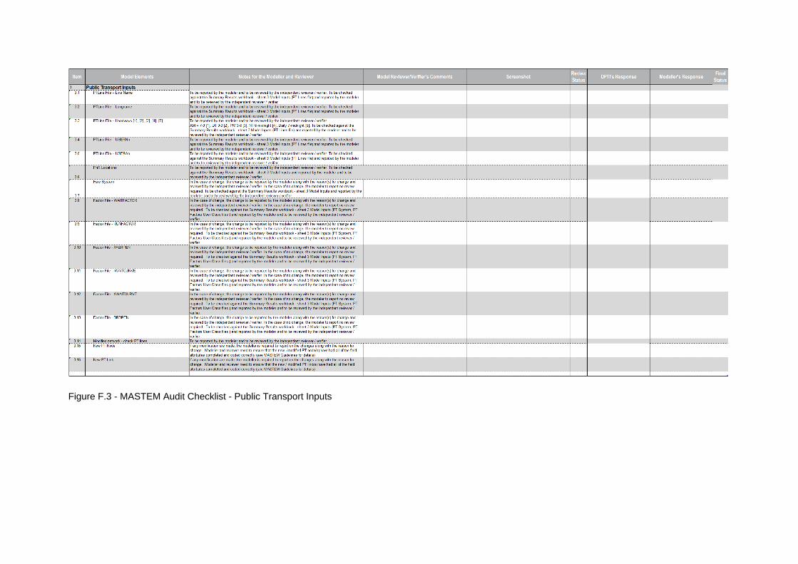
Figure F.3 - MASTEM Audit Checklist - Public Transport Inputs


![ADELAIDE, AUSTRALIAonlinepubs.trb.org/onlinepubs/tcrp/tcrp90v1_cs/Adelaide.pdf · Metropolitan Adelaide has a population of 1.1 million. The urban area is 80 kilometers [50 miles]](https://img.pdfslide.us/doc/110x75/5f042fcf7e708231d40cbdae/adelaide-metropolitan-adelaide-has-a-population-of-11-million-the-urban-area.jpg)


![BANGALORE METROPOLITAN TRANSPORT …...1 BANGALORE METROPOLITAN TRANSPORT CORPORATION RTI UNDER [Section 4(1) B] CHAPTER-16 PERSONNEL DEPARTMENT Information about the Public Information](https://img.pdfslide.us/doc/110x75/5e73911ea9d9e6018977d59e/bangalore-metropolitan-transport-1-bangalore-metropolitan-transport-corporation.jpg)