10 Metric Path Planning

Chapter objectives:

Define Cspace, path relaxation, digitization bias, subgoal obsession, terminationcondition.

Explain the difference between graph and wavefront planners.

Represent an indoor environment with a generalized Voronoi graph, a regu-lar grid, or a quadtree, and create a graph suitable for path planning.

Apply the A* search algorithm to a graph to find the optimal path betweentwo locations.

Apply wavefront propagation to a regular grid.

Explain the differences between continuous and event-driven replanning.

10.1 Objectives and Overview

Metric path planning, or quantitative navigation, is the opposite of topologi-QUANTITATIVE

NAVIGATION cal navigation. As with topological methods, the objective is to determinea path to a specified goal. The major philosophical difference is that metricmethods generally favor techniques which produce an optimal, according tosome measure of best, while qualitative methods seem content to producea route with identifiable landmarks or gateways. Another difference is thatmetric paths are usually decompose the path into subgoals consisting of way-WAYPOINTS

points. These waypoints are most often a fixed location or coordinate (x,y).These locations may have a mathematical meaning, but as will be seen withmeadow maps, they may not have a sensible correspondence to objects or

352 10 Metric Path Planning

landmarks in the world. Topological navigation focused on subgoals whichare gateways or locations where the robot could change its primary heading.

The terms “optimal” and “best” have serious ramifications for robotics.In order to say a path is optimal, there is an implied comparison. As willbe seen, some metric methods are able to produce an optimal path becausethey consider all possible paths between points. This can be computationallyexpensive. Fortunately, some algorithms (especially one named “A*” for rea-sons that will be discussed later) are more clever about rejecting non-optimalpaths sooner than others.

Surprisingly, an optimal path may not appear optimal to the human eye;for example, a mathematically optimal path of a world divided into tiles orgrids may be very jagged and irregular rather than straight. The ability toproduce and compare all possible paths also assumes that the planning hasaccess to a pre-exisiting (or a priori) map of the world. Equally as important,it assumes that the map is accurate and up to date. As such, metric methodsare compatible with deliberation, while qualitative methods work well withmore reactive systems. As a deliberative function, metric methods tend tobe plagued by the same sorts of difficulties that were seen in Hierarchicalsystems: challenges in world representation, handling dynamic changes andsurprises, and computation complexity.

Metric path planners have two components: the representation (data struc-COMPONENTS OF

METRIC PATH

PLANNERSture) and the algorithm. Path planners first partition the world into a structureamenable for path planning. They use a variety of techniques to representthe world; no one technique is dominant, although regular grids appear tobe popular. The intent of any representation is to represent only the salientfeatures, or the relevant configuration of navigationally relevant objects inthe space of interest; hence the term configuration space. Path planning al-gorithms generally work on almost any configuration space representation,although as with any algorithm, some methods work better on certain datastructures. The algorithms fall into two broad categories: those which treatpath planning as a graph search problem, and those which treat path plan-ning as a graphics coloring problem. Regardless of what algorithm is used,there is always the issue in a Hybrid architecture of when to use it. This issometimes called the issue of interleaving reaction and planning.

10.2 Configuration Space 353

Figure 10.1 Reduction of a 6DOF world space to a 2DOF configuration space.

10.2 Configuration Space

The physical space robots and obstacles exist in can be thought of as theworld space. The configuration space, or Cspace for short, is a data structureCONFIGURATION SPACE

which allows the robot to specify the position (location and orientation) ofany objects and the robot.

A good Cspace representation reduces the number of dimensions that aplanner has to contend with. Consider that it takes six dimensions (alsocalled degrees of freedom or DOF) to represent precisely where an object is. ADEGREES OF FREEDOM

person may specify the location of the object as a coordinate in someframe of reference. But an object is three-dimensional; it has a front and back,top and bottom. Three more degrees are needed to represent where the frontof the chair is facing, whether it is tilted or not, or even upside down. Thoseare the Euler (pronounced “Oiler”) angles, , also known as pitch, yaw,and roll.

Six degrees of freedom is more than is needed for a mobile ground robot inmost cases for planning a path. The (height) coordinate can be eliminatedif every object the robot sits on the floor. However, the coordinate will beof interest if the robot is an aerial or underwater vehicle. Likewise, the Eulerangles may be unnecessary. Who cares which way the robot is facing if allthe robot wants to do is to plan a path around it? But the pitch of a planetaryrover or slope of an upcoming hill may be critical to a mission over rockyterrain.

Fig. 10.1 shows a transformation of an object into Cspace. In general, met-ric path planning algorithms for mobile robots have assumed only two DOF,including for the robot. For path planning purposes, the robot can be mod-eled as round so that the orientation doesn’t matter. This implicitly assumes

354 10 Metric Path Planning

the robot is holonomic, or can turn in place. Many research robots are suffi-HOLONOMIC

ciently close to holonomic to meet this assumption. However, robots madefrom radio-controlled cars or golf carts are most certainly not holonomic.Much work is being done in non-holonomic path planning, where the poseof the robot must be considered (i.e., can it actually turn that sharply withoutcolliding?), but there no one algorithm appears to be used in practice. Thischapter will restrict itself to holonomic methods.

10.3 Cspace Representations

The number of different Cspace representations is too large to include morethan a coarse sampling here. The most representative ones are Voronoi di-agrams, regular grids, quadtrees (and their 3D extension, octrees), vertexgraphs, and hybrid free space/vertex graphs. The representations offer dif-ferent ways of partitioning free space. Any open space not occupied by anobject (a wall, a chair, an un-navigable hill) is free space, where the robot isfree to move without hitting anything modeled. Each partition can be la-beled with additional information: “the terrain is rocky,” “this is off-limitsfrom 9am to 5am,” etc.

10.3.1 Meadow maps

Many early path planning algorithms developed for mobile robots assumedthat the robot would have a highly accurate map of the world in advance.This map could be digitized in some manner, and then the robot could applyvarious algorithms to convert the map to a suitable Cspace representation.An example of a Cspace representation that might be used with an a priorimap is the meadow map or hybrid vertex-graph free-space model.MEADOW MAP

Meadow maps transform free space into convex polygons. Convex poly-gons have an important property: if the robot starts on the perimeter andgoes in a straight line to any other point on the perimeter, it will not go out ofthe polygon. The polygon represents a safe region for the robot to traverse.The path planning problem becomes a matter of picking the best series ofpolygons to transit through. Meadow maps are not that common in robotics,but serve to illustrate the principles of effecting a configuration space andthen planning a path over it.

The programming steps are straightforward. First, the planner begins witha metric layout of the world space. Most planners will increase the size ofevery object by the size of the robot as shown in Fig. 10.2; this allows the

10.3 Cspace Representations 355

Figure 10.2 A a priori map, with object boundaries “grown” to the width of the robot(shown in gray).

a. b.

Figure 10.3 Meadow maps: a.) partitioning of free space into convex polygons, andb.) generating a graph using the midpoints.

planner to treat the robot as if it were a point, not a 2D object. Notice howfrom the very first step, path planners assume holonomic vehicles.

The next step in the algorithm is to construct convex polygons by consid-ering the line segments between pairs of some interesting feature. In the caseof indoor maps, these are usually corners, doorways, boundaries of objects,etc. The algorithm can then determine which combination of line segmentspartitions the free space into convex polygons.

The meadow map is now technically complete, but it is not in a format thatsupports path planning. Each convex polygon represents a safe passage forthe robot. But there is still some work to be done. Some of the line segments

356 10 Metric Path Planning

Figure 10.4 String tightening as a relaxation of an initial path.

forming the perimeter aren’t connected to another a polygon (i.e., they arepart of a wall), so they should be off limits to the planning algorithm. Also,as can be seen by the above figure, some of the line segments are quite long.It would make a difference to the overall path length where the robot cutsacross the polygon. It is hard for the planner to discretize a continuous linesegment. So the issue becomes how to specify candidate points on the poly-gon. One solution is to find the middle of each line segment which bordersanother polygon. Note that each of these midpoints becomes a node, andif edges are drawn between them, an undirected graph emerges. A pathplanning algorithm would determine the best path to take.

One disadvantage of a meadow map, indeed of any Cspace representa-tion, is evident on inspection of Fig. 10.3: any path which is chosen will besomewhat jagged. Each of the inflection points is essentially a waypoint.One outcome of the partitioning process is that the free space is divided upin a way that makes sense geometrically, but not necessarily for a robot toactually travel. Why go halfway down the hall, then angle off? This may bemathematically optimal on paper, but in practice, it seems downright silly.Chuck Thorpe at CMU devised a solution to paths generated from any kindof discretization of free space.138 Imagine that the path is a string. Now imag-ine pulling on both ends to tighten the string (the technical name for this ispath relaxation) This would remove most of the kinks from the path withoutPATH RELAXATION

violating the safe zone property of convex polygons.Meadow maps have three problems which limit their usefulness. One

problem is that the technique to generate the polygons is computationally

10.3 Cspace Representations 357

Figure 10.5 Graph from a generalized Voronoi graph (GVG). (Graph courtesy ofHowie Choset.)

complex. But more importantly, it uses artifacts of the map to determine thepolygon boundaries, rather than things which can be sensed. Unless the ro-bot has accurate localization, how does it know it is halfway down a long,featureless hall and should turn ? The third major disadvantage is thatit is unclear how to update or repair the diagrams as the robot discoversdiscrepancies between the a priori map and the real world.

10.3.2 Generalized Voronoi graphs

Generalized Voronoi Graphs, or GVGs, are a popular mechanism for represent-GENERALIZED

VORONOI GRAPHS ing Cspace and generating a graph. Unlike a meadow map, a GVG can beconstructed as the robot enters a new environment, thereby creating a topo-logical map as shown by Howie Choset at CMU.36

The basic idea of a GVG is to generate a line, called a Voronoi edge, equidis-VORONOI EDGE

tant from all points. As seen in Fig. 10.5, this line goes down the middle ofhallways and openings. The point where many Voronoi edges meet is knownas a Voronoi vertex. Notice the vertices often have a physical correspondenceto configurations that can be sensed in the environment. This makes it mucheasier for a robot to follow a path generated from a GVG, since there is animplicit local control strategy of staying equidistant from all obstacles.

If the robot follows the Voronoi edge, it will not collide with any modeledobstacles, because it is staying “in the middle.” This obviates the need togrow the obstacle boundaries. Edges serve as freeways or major thorough-

358 10 Metric Path Planning

Figure 10.6 Regular grid.

fares. It should also be noted that the curved edges in a GVG do not matterto graph theory or graph algorithms. It is only the length, not the physicalreality, of the edges that make any difference.

10.3.3 Regular grids

Another method of partitioning the world space is a regular grid. The regulargrid method superimposes a 2D Cartesian grid on the world space, as shownin Fig. 10.6. If there is any object in the area contained by a grid element, thatelement is marked occupied. Hence, regular grids are often referred to asoccupancy grids. Occupancy grids will be detailed in Ch. 11.

Regular grids are straightforward to apply. The center of each elementin the grid can become a node, leading to a highly connected graph. Gridsare either considered 4-connected or 8-connected, depending on whether they4-CONNECTED

NEIGHBORS

8-CONNECTED

NEIGHBORS

permit an arc to be drawn diagonally between nodes or not.Unfortunately, regular grids are not without problems. First, they intro-

duce digitization bias, which means that if an object falls into even the smallestDIGITIZATION BIAS

portion of a grid element, the whole element is marked occupied. This leadsto wasted space and leads to very jagged objects. To reduce the wasted space,regular grids for an indoor room are often finely grained, on the order of 4- to6-inches square. This fine granularity means a high storage cost, and a highnumber of nodes for a path planning algorithm to consider.

10.4 Graph Based Planners 359

Figure 10.7 Quadtree Cspace representation.

10.3.4 Quadtrees

A variant on regular grids that attempts to avoid wasted space is quadtrees.QUADTREES

Quadtrees are a recursive grid. The representation starts out with grid el-ements representing a large area, perhaps 64-inches square (8 by 8 inches).If an object falls into part of the grid, but not all of it, the Cspace algorithmdivides the element into four (hence the name “quad”) smaller grids, each 16-inches square. If the object doesn’t fill a particular sub-element, the algorithmdoes another recursive division of that element into four more sub-elements,represented a 4-inches square region. A three dimensional quadtree is calledan octree.

10.4 Graph Based Planners

As seen in the previous section, most Cspace representations can be con-verted to graphs. This means that the path between the initial node and theINITIAL NODE

goal node can be computed using graph search algorithms. Graph search al-GOAL NODE

gorithms appear in networks and routing problems, so they form a class ofalgorithms well understood by computer science. However, many of thosealgorithms require the program to visit each node on the graph to determinethe shortest path between the initial and goal nodes. Visiting every node maybe computationally tractable for a sparsely connected graph such as derivedfrom a Voronoi diagram, but rapidly becomes computationally expensive fora highly connected graph such as from a regular grid. Therefore, there has

360 10 Metric Path Planning

been a great deal of interest in path planners which do a “branch and bound”style of search; that is, ones which prune off paths which aren’t optimal. Ofcourse, the trick is knowing when to prune!

The A* search algorithm is the classic method for computing optimal pathsfor holonomic robots. It is derived from the A search method. In order toexplain how A* works, A search will be first presented with an example, thenA*. Both assume a metric map, where the location of each node is known inabsolute coordinates, and the graph edges represent whether it is possible totraverse between those nodes.

The A search algorithm produces an optimal path by starting at the initialnode and then working through the graph to the goal node. It generates theoptimal path incrementally; each update, it considers the nodes that couldbe added to the path and picks the best one. It picks the “right” node to addto the path every time it expands the path (the "right node” is more formallyknown as the plausible move). The heart of the method is the formula (orevaluation function) for measuring the plausibility of a node:

where:

measures how good the move to node is

measures the cost of getting to node from the initial node. Since Aexpands from the initial node outward, this is just the distance of the pathgenerated so far plus the distance of the edge to node

is the cheapest cost of getting from to goal

Consider how the formula is used in the example below. Assume that aCspace representation yielded the graph in Fig. 10.8.

The A search algorithm begins at node , and creates a decision tree-likestructure to determine which are the possible nodes it can consider addingto its path. There are only two nodes to choose from: B and C.

In order to determine which node is the right node to add, the A searchalgorithm evaluates the plausibility of B and C by looking at the edges. Theplausibility of B as the next move is:

where is the cost of going from to , and is the cost to get fromto the goal .

10.4 Graph Based Planners 361

Figure 10.8 Graph for A search algorithm.

The plausibility of is:

where is the cost of going from to , and is the cost of gettingfrom to . Since , the path should go from to .

But this assumes that was known at every node. This meant that thealgorithm had to recurse in order to find the correct value of . This leadsto visiting all the nodes.

A search is guaranteed to produce the optimal path because it comparesall possible paths to each other. A* search takes an interesting approach toreducing the amount of paths that have to be generated and compared: itcompares the possible paths to the best possible path, even if there isn’t apath in the real world that goes that way. The algorithm estimates ratherthan checks to see if there is actually a path segment that can get to the goal inthat distance. The estimate can then be used to determine which nodes arethe most promising, and which paths have no chance of reaching the goalbetter than other candidates and should be pruned from the search.

Under A* the evaluation function becomes:

where the means that the functions are estimates of the values that would

362 10 Metric Path Planning

Figure 10.9 An A* example.

have been plugged into the A search evaluation. In path planning,is the same as : the cost of getting from the initial node to n, which isknown through the incremental build of the path. is the real difference.So what is a way to estimate the cost of going from to the goal? Further-more, how can we be sure that the estimate will be accurate enough that wedon’t end up choosing a path which isn’t truly optimal? This can be done bymaking sure that will never be smaller than . The restriction that

is called the admissibility condition. Since is an estimate, itADMISSIBILITY

CONDITION is also called a heuristic function, since it uses a rule of thumb to decide whichHEURISTIC FUNCTION is the best node to consider.

Fortunately, there is a natural heuristic function for estimating the costfrom n to the goal: the Euclidean (straight line) distance. Recall that thelocations of each node are known independently of the edges. Therefore, itis straightforward to compute the straight line distance between two nodes.The straight line distance is always the shortest path between two points,barring curvature of the earth, etc. Since the real path can never be shorterthan that, the admissibility condition is satisfied.

To see how A* uses this to actually eliminate visiting nodes, consider theexample in Fig. 10.9. As with A search, the first step in A* is to consider thechoices from the initial node.

The choices are and , which can be thought of as a search tree (seeFig. 10.10a) or as a subset of the original graph (see Fig 10.10b). Regardless

10.4 Graph Based Planners 363

Figure 10.10 a.) What A* “sees” as it considers a path A-?-E, and b.) the originalgraph. c.) What A* “sees” from considering a path A-D-?-E, and d.) the associatedgraph.

364 10 Metric Path Planning

of how it is visualized, each node is evaluated to determine which is themost plausible move. The above figure shows what the algorithm “sees” atthis point in the execution. The choices evaluate to:

A path going from has the potential to be shorter than apath going from . So, is the most plausible node. Noticethat A* can’t eliminate a path through because the algorithm can’t “see” apath that actually goes from to and determine if it is indeed as short aspossible.

At step 2, A* recurses (repeats the evaluation) from , since is the mostplausible, as shown in Fig. 10.10.

The two options from are and , which are evaluated next:

Now the algorithm sees that is the best choice among the leaves of thesearch tree, including the branch through . (If was the best, then thealgorithm would have changed branches.) It is better than and . When itgoes to expand , it notices that is the goal, so the algorithm is complete.The optimal path is , and we didn’t have to explicitly consider

. There are other ways to improve the procedure describedso far. didn’t need to be computed if the algorithm looks at its choicesand sees that one of them is the goal. Any other choice has to be longerbecause edges aren’t allowed to be negative, so has to be longerthan .

Another important insight is that any path between and has to gothrough , so the branch of the search tree could have been pruned. Ofcourse, in the above example the algorithm never had an opportunity to no-tice this because was never expanded. It’s easy to imagine in a larger graphthat there might be a case where after several expansions through , the leafat in the search tree came up the most plausible. Then the algorithm wouldhave expanded and seen the choices were . Since already occurred inanother branch, with a cheaper , the branch could be safely pruned.

10.5 Wavefront Based Planners 365

This is particularly useful when A* is applied to a graph created from a reg-ular grid, where the resulting graph is highly connected.

One very attractive feature of the A* path planner is that it can be usedwith any Cspace representation that can be transformed into a graph. Themajor impact that Cspace has on the A* planner is how many computationsit takes to find the path.

A limitation of A* is that it is very hard to use for path planning wherethere are factors other than distance to consider in generating the path. Forexample, the straight line distance may be over rocky terrain or sand thatposes a risk to the robot. Likewise, the robot may wish to avoid going overhills in order to conserve energy, but at the same time might wish to go downhills whenever possible for the same reason. In order to factor in the impactof terrain on the path costs, the heuristic function has to be changed.But recall that the new heuristic function must continue to satisfy the admis-sibility condition: . If the new just takes the worst case energy costor safety cost, it will be admissible, but not particularly useful in pruningpaths. Also, gaining energy going downhill is essentially having an edge inthe graph with a negative weight, which A* can’t handle. (Negative weightspose an interesting problem in that the robot can get into a loop of rollingdown a hill repeatedly because it’s an energy-efficient solution rather thanactually making forward progress! Bellman-Ford types of algorithms dealwith this situation.)

10.5 Wavefront Based Planners

Wavefront propagation styles of planners are well suited for grid types ofrepresentations. The basic principle is that a wavefront considers the Cspaceto be a conductive material with heat radiating out from the initial node tothe goal node. Eventually the heat will spread and reach the goal, if thereis a way, as shown in the sequence in Fig. 10.11. Another analogy for wave-front planners is region coloring in graphics, where the color spreads out toneighboring pixels. An interesting aspect of wavefront propagation is thatthe optimal path from all grid elements to the goal can be computed as aside effect. The result is a map which looks like a potential field. One of themany wavefront types of path planners is the Trulla algorithm developedby Ken Hughes.106 It exploits the similarities with a potential field to let thepath itself represent what the robot should do as if the path were a sensorobservation.

366 10 Metric Path Planning

a. b.

c. d.

e. f.

g. h.

Figure 10.11 A wave propagating through a regular grid. Elements holding thecurrent front are shown in gray, older elements are shown in dark gray.

10.6 Interleaving Path Planning and Reactive Execution 367

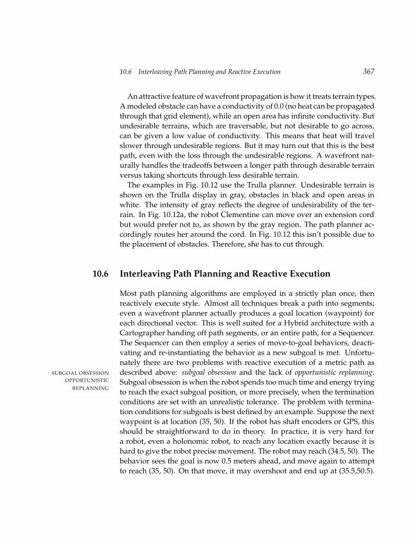
An attractive feature of wavefront propagation is how it treats terrain types.A modeled obstacle can have a conductivity of 0.0 (no heat can be propagatedthrough that grid element), while an open area has infinite conductivity. Butundesirable terrains, which are traversable, but not desirable to go across,can be given a low value of conductivity. This means that heat will travelslower through undesirable regions. But it may turn out that this is the bestpath, even with the loss through the undesirable regions. A wavefront nat-urally handles the tradeoffs between a longer path through desirable terrainversus taking shortcuts through less desirable terrain.

The examples in Fig. 10.12 use the Trulla planner. Undesirable terrain isshown on the Trulla display in gray, obstacles in black and open areas inwhite. The intensity of gray reflects the degree of undesirability of the ter-rain. In Fig. 10.12a, the robot Clementine can move over an extension cordbut would prefer not to, as shown by the gray region. The path planner ac-cordingly routes her around the cord. In Fig. 10.12 this isn’t possible due tothe placement of obstacles. Therefore, she has to cut through.

10.6 Interleaving Path Planning and Reactive Execution

Most path planning algorithms are employed in a strictly plan once, thenreactively execute style. Almost all techniques break a path into segments;even a wavefront planner actually produces a goal location (waypoint) foreach directional vector. This is well suited for a Hybrid architecture with aCartographer handing off path segments, or an entire path, for a Sequencer.The Sequencer can then employ a series of move-to-goal behaviors, deacti-vating and re-instantiating the behavior as a new subgoal is met. Unfortu-nately there are two problems with reactive execution of a metric path asdescribed above: subgoal obsession and the lack of opportunistic replanning.SUBGOAL OBSESSION

OPPORTUNISTIC

REPLANNINGSubgoal obsession is when the robot spends too much time and energy tryingto reach the exact subgoal position, or more precisely, when the terminationconditions are set with an unrealistic tolerance. The problem with termina-tion conditions for subgoals is best defined by an example. Suppose the nextwaypoint is at location (35, 50). If the robot has shaft encoders or GPS, thisshould be straightforward to do in theory. In practice, it is very hard fora robot, even a holonomic robot, to reach any location exactly because it ishard to give the robot precise movement. The robot may reach (34.5, 50). Thebehavior sees the goal is now 0.5 meters ahead, and move again to attemptto reach (35, 50). On that move, it may overshoot and end up at (35.5,50.5).

368 10 Metric Path Planning

a.

b.

Figure 10.12 a.) Trulla output and photo of Clementine navigating around cord. b.)Trulla output and photo of Clementine navigating over the cord.

Now it has to turn and move again. A resulting see-sawing set of motionsemerges that can go on for minutes. This wastes time and energy, as well asmakes the robot appear to be unintelligent. The problem is exacerbated bynon-holonomic vehicles which may have to back up in order to turn to reacha particular location. Backing up almost always introduces more errors innavigation.

To handle subgoal obsession, many roboticists program into their move-to-goal behaviors a tolerance on the terminating condition for reaching a goal.A common heuristic for holonomic robots is to place a tolerance of +/- thewidth of the robot. So if a cylindrical, holonomic robot with a diameter of 1meter is given a goal of (35, 50), it will stop when 34.5 35.5 and 49.5

10.6 Interleaving Path Planning and Reactive Execution 369

50.5. There is no common heuristic for non-holonomic robots, becausethe maneuverability of each platform is different. A more vexing aspect ofsubgoal obsession is when the goal is blocked and the robot can’t reach theterminating condition. For example, consider a subgoal at the opposite endof a hall from a robot, but the hall is blocked and there is no way around.Because the robot is executing reactively, it doesn’t necessarily realize that itisn’t making progress. One solution is for the Sequencer to estimate a maxi-mum allowable time for the robot to reach the goal. This can be implementedeither as a parameter on the behavior (terminate with an error code afterseconds), or as an internal state releaser. The advantage of the latter solu-tion is that the code can become part of a monitor, leading to some form ofself-awareness.

Related to subgoal obsession is the fact that reactive execution of plansoften lacks opportunistic improvements. Suppose that the robot is headingfor Subgoal 2, when an unmodeled obstacle diverts the robot from its in-tended path. Now suppose that from its new position, the robot can perceiveSubgoal 3. In a classic implementation, the robot would not be looking forSubgoal 3, so it would continue to move to Subgoal 2 even though it wouldbe more optimal to head straight for Subgoal 3.

The need to opportunistically replan also arises when an a priori map turnsout to be incorrect. What happens when the robot discovers it is being sentthrough a patch of muddy ground? Trying to reactively navigate aroundthe mud patch seems unintelligent because choosing left or right may haveserious consequences. Instead the robot should return control to the Car-tographer, which will update its map and replan. The issue becomes howdoes a robot know it has deviated too far from its intended path and needsto replan?

Two different types of planners address the problems of subgoal obses-sion and replanning: the D* algorithm developed by Tony Stentz136 which isD* ALGORITHM

a variant of the A* replanning algorithm, and an extension to the Trulla al-gorithm. Both planners begin with an a priori map and compute the optimalpath from every location to the goal. D* does it by executing an A* searchfrom each possible location to the goal in advance; this converts A* from be-ing a single-source shortest path algorithm into an all-paths algorithm. Thisis computationally expensive and time-consuming, but that isn’t a problemsince the paths are computed when the robot starts the mission and is sittingstill. Since Trulla is a wavefront type of planner, it generates the optimal pathbetween all pairs of points in Cspace as a side effect of computing the pathfrom the starting location to the goal.

370 10 Metric Path Planning

start

unmodeledobstacle

goal

a.

b.

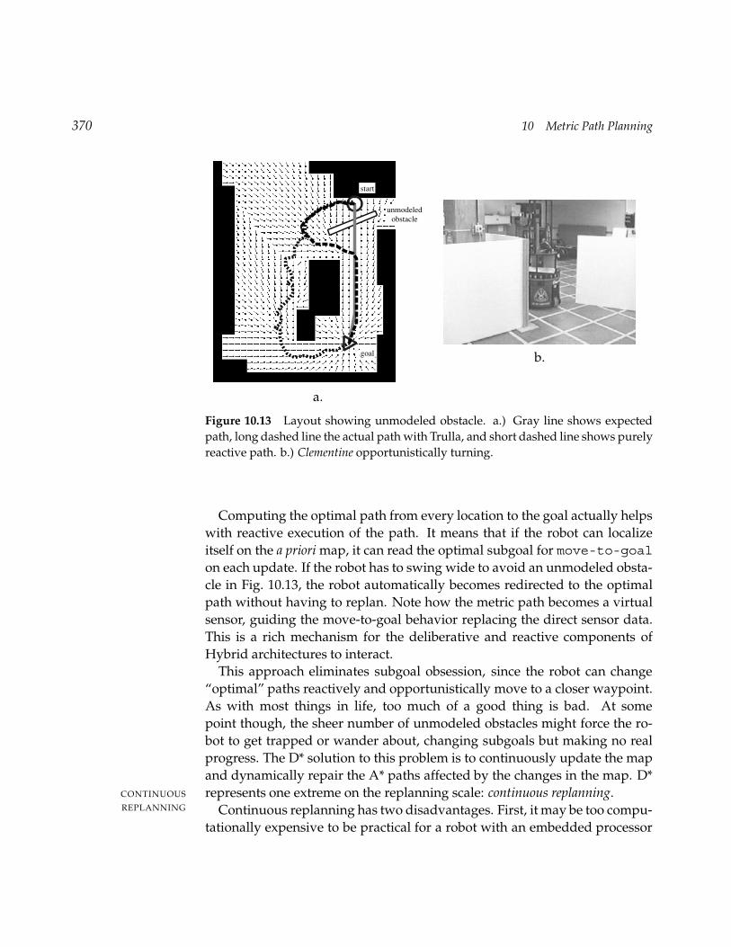
Figure 10.13 Layout showing unmodeled obstacle. a.) Gray line shows expectedpath, long dashed line the actual path with Trulla, and short dashed line shows purelyreactive path. b.) Clementine opportunistically turning.

Computing the optimal path from every location to the goal actually helpswith reactive execution of the path. It means that if the robot can localizeitself on the a priori map, it can read the optimal subgoal for move-to-goalon each update. If the robot has to swing wide to avoid an unmodeled obsta-cle in Fig. 10.13, the robot automatically becomes redirected to the optimalpath without having to replan. Note how the metric path becomes a virtualsensor, guiding the move-to-goal behavior replacing the direct sensor data.This is a rich mechanism for the deliberative and reactive components ofHybrid architectures to interact.

This approach eliminates subgoal obsession, since the robot can change“optimal” paths reactively and opportunistically move to a closer waypoint.As with most things in life, too much of a good thing is bad. At somepoint though, the sheer number of unmodeled obstacles might force the ro-bot to get trapped or wander about, changing subgoals but making no realprogress. The D* solution to this problem is to continuously update the mapand dynamically repair the A* paths affected by the changes in the map. D*represents one extreme on the replanning scale: continuous replanning.CONTINUOUS

REPLANNING Continuous replanning has two disadvantages. First, it may be too compu-tationally expensive to be practical for a robot with an embedded processor

10.7 Summary 371

and memory limitations, such as a planetary rover. Second, continuous re-planning is highly dependent on the sensing quality. If the robot senses anunmodeled obstacle at time T1, it computes a new path and makes a largecourse correction. If it no longer senses that obstacle at time T2 because thefirst reading was a phantom from sensor noise, it will recompute anotherlarge course correction. The result can be a robot which has a very jerkymotion and actually takes longer to reach the goal.

In the cases of path planning with embedded processors and noisy sensors,it would be desirable to have some sort of event-driven scheme, where anEVENT-DRIVEN

REPLANNING event noticeable by the reactive system would trigger replanning. Trulla usesthe dot-product of the intended path vector and the actual path vector. Whenthe actual path deviates by or more, the dot product of the path vectorand the actual vector the robot is following becomes 0 or negative. Thereforethe dot product acts as an affordance for triggering replanning: the robotdoesn’t have to know why it is drifting off-course, only that it has driftednoticeably off-course.

This is very good for situations that would interfere with making progresson the originally computed path, in effect, situations where the real worldis less amenable to reaching the intended goal. But it doesn’t handle thesituation where the real world is actually friendlier. In Fig. 10.14, an obstaclethought to be there really isn’t. The robot could achieve a significant savingsin navigation by opportunistically going through the gap.

Such opportunism requires the robot to notice that the world is reallymore favorable than originally modeled. A continuous replanner such as D*has a distinct advantage, since it will automatically notice the change in theworld and respond appropriately, whereas Trulla will not notice the favor-able change because it won’t lead to a path deviation. It is an open researchquestion whether there are affordances for noticing favorable changes in theworld that allow the robot to opportunistically optimize it path.

10.7 Summary

Metric path planning converts the world space to a configuration space, orCspace, representation that facilitates path planning. Cspace representationssuch as generalized Voronoi diagrams exploit interesting geometric prop-erties of the environment. These representations can then be converted tographs, suitable for an A* search. Since Voronoi diagrams tend to producesparser graphs, they work particularly well with A*. Regular grids work

372 10 Metric Path Planning

start

goal

missingwall

Figure 10.14 Opportunity to improve path. The gray line is the actual path, whilethe dashed line represents a more desirable path.

well with wavefront planners, which treat path planning as an expandingheat wave from the initial location.

Metric path planning tends to be expensive, both in computation and instorage. However, they can be interleaved with the reactive component ofa Hybrid architecture, where the Cartographer gives the Sequencer a set ofwaypoints. Two problems in interleaving metric path planning with reactiveexecution are subgoal obsession and when to replan. Optimal path planningtechniques for a priori fixed maps are well understood, but it is less clear howto update or repair the path(s) without starting over if the robot encountersa significant deviation from the a priori map. One solution is to continuouslyreplan if resources permit and sensor reliability is high; another is event-driven replanning which uses affordances to detect when to replan.

Cspace representations and algorithms often do not consider how to rep-resent and reason about terrain types, and special cases such as the robot ac-tually conserving or generating energy going downhill are usually ignored.A possibly even more serious omission is that popular path planners areapplicable for only holonomic vehicles.

10.8 Exercises

Exercise 10.1

Represent your indoor environment as a GVG, regular grid, and quadtree.

10.8 Exercises 373

Exercise 10.2

Represent your indoor environment as a regular grid with a 10cm scale. Write downthe rule you use to decide how to mark a grid element empty or occupied when thereis a small portion overlapping it.

Exercise 10.3

Define path relaxation.

Exercise 10.4

Consider a regular grid of size 20 by 20. How many edges will a graph have if theneighbors are

a. 4-connected?

b. 8-connected?

Exercise 10.5

Convert a meadow map into a graph using:

a. the midpoints of the open boundaries, and

b. the midpoints plus the 2 endpoints.

Draw a path from A to B on both graphs. Describe the differences.

Exercise 10.6

Apply the A* search algorithm by hand to a small graph to find the optimal pathbetween two locations.

Exercise 10.7

What is a heuristic function?

Exercise 10.8

Apply wavefront propagation to a regular grid.

Exercise 10.9

Subgoal obsession has been described as a problem for metric planners. Can hybridsystems which use topological planning exhibit subgoal obsession?

Exercise 10.10

Trulla uses a dot product of 0 or less to trigger replanning, which corresponds tofrom the desired path. What are the advantages or disadvantages of ? What

would happen if Trulla used or ?

Exercise 10.11

Describe the difference between continuous and event-driven replanning. Which wouldbe more appropriate for a planetary rover? Justify your answer.

374 10 Metric Path Planning

Exercise 10.12 [Programming]Obtain a copy of the Trulla simulator suitable for running under Windows. Model atleast three different scenarios and see what the path generated is.

Exercise 10.13 [Programming]Program an A* path planner. Compare the results to the results for the Dijkstra’ssingle source shortest path program from Ch. 9.

10.9 End Notes

For a roboticist’s bookshelf.Robot Motion Planning by Jean-Claude Latombe of Stanford University is the best-known book dealing with configuration space. 82

Voronoi diagrams.Voronoi diagrams may be the oldest Cspace representation. Computational Geometry:Theory and Applications 44 reports that the principles were first uncovered in 1850, al-though it wasn’t until 1908 that Voronoi wrote about them, thereby getting his nameon the diagram.

On heuristic functions for path planning.Kevin Gifford and George Morgenthaler have explored some possible formulationsof a heuristic function for path planning over different terrain types. Gifford alsodeveloped an algorithm which can consider the energy savings or capture associatedwith going downhill. 60

Trulla.The Trulla algorithm was developed by Ken Hughes for integration on a VLSI chip.Through grants from the CRA Distributed Mentoring for Women program, Eva Nolland Aliza Marzilli implemented it in software. The algorithm was found to work fastenough for continuous updating even on an Intel 486 processor. Dave Hershbergerhelped write the display routines used in this book.