METO 621

Lesson 14

Prototype Problem I: Differential Equation Approach

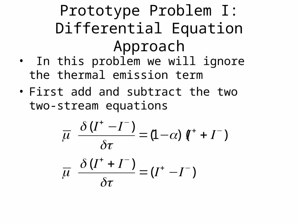
• In this problem we will ignore the thermal emission term

• First add and subtract the two two-stream equations

)()(

))(1()(

−+−+

−+−+

−=+

+−=−

IId

IId

IIad

IId

τμ

τμ

Prototype Problem I

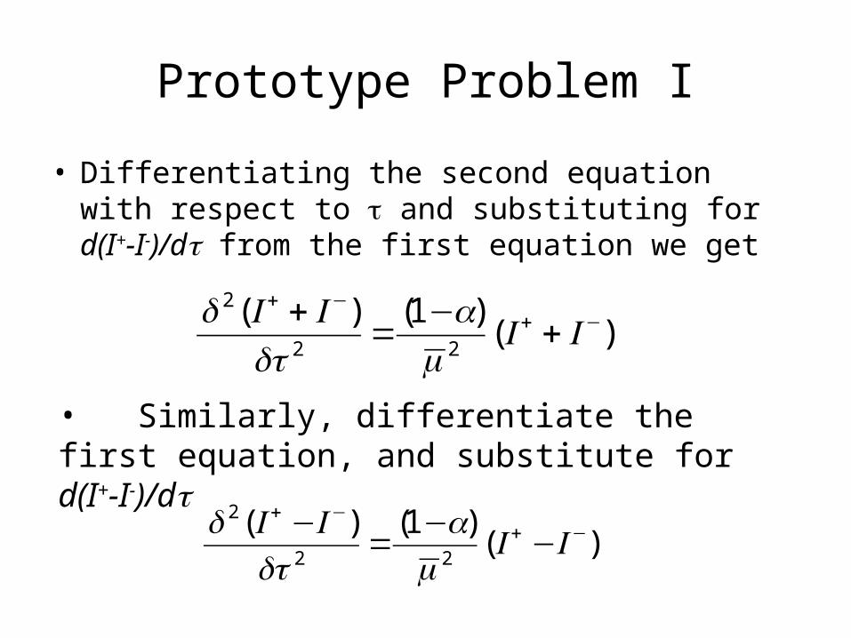
• Differentiating the second equation with respect to τ and substituting for d(I+-I-)/dτ from the first equation we get

)()1()(

22

2−+

−+

+−

=+

IIa

dIId

μτ• Similarly, differentiate the first equation, and substitute for d(I+-I-)/dτ

)()1()(

22

2−+

−+

−−

=−

IIa

dIId

μτ

Prototype Problem I

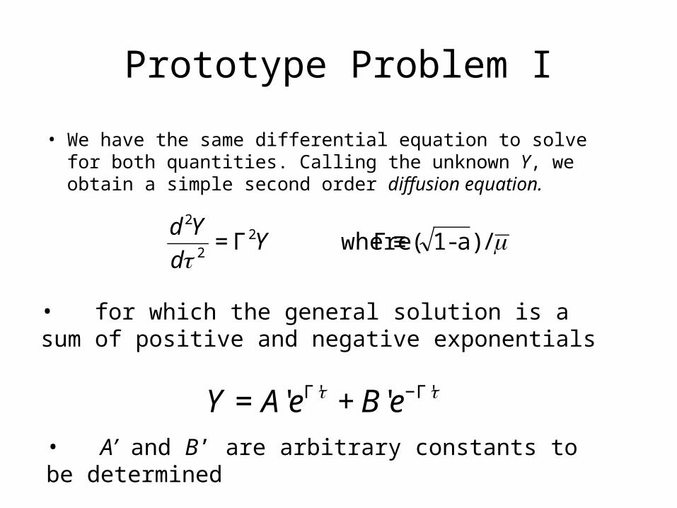
• We have the same differential equation to solve for both quantities. Calling the unknown Y, we obtain a simple second order diffusion equation.

μτ

/)a-1( where22

2

≡ΓΓ= Yd

Yd

• for which the general solution is a sum of positive and negative exponentials

ττ '' '' Γ−Γ += eBeAY• A’ and B’ are arbitrary constants to be determined

Prototype Problem I

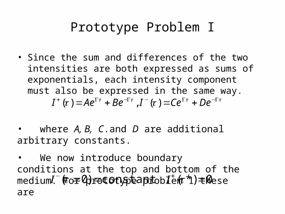
• Since the sum and differences of the two intensities are both expressed as sums of exponentials, each intensity component must also be expressed in the same way.

ττττ ττ Γ−Γ−Γ−Γ+ +=+= DeCeIBeAeI )( ,)(

• where A, B, C.and D are additional arbitrary constants.

• We now introduce boundary conditions at the top and bottom of the medium. For prototype problem 1 these are

0*)( constant )0( === +− ττ II

Prototype Problem I

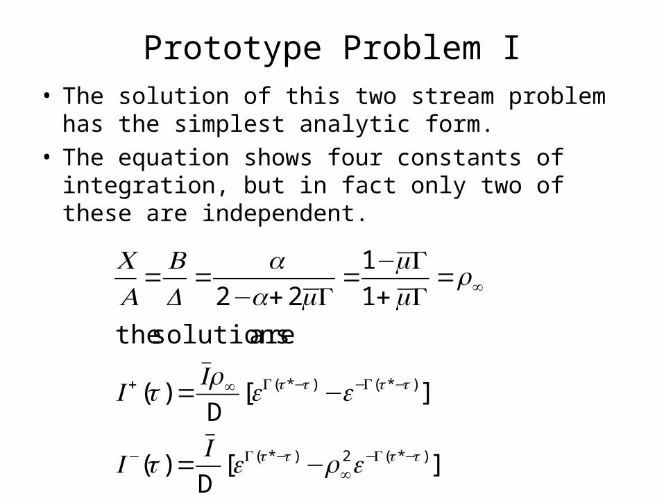
• The solution of this two stream problem has the simplest analytic form.

• The equation shows four constants of integration, but in fact only two of these are independent.

][)(

][)(

are solutions the

1

1

22

)*(2)*(

)*()*(

ττττ

ττττ

ρτ

ρτ

ρμμ

μ

−Γ−∞

−Γ−

−Γ−−Γ∞+

∞

−=

−=

=Γ+Γ−

=Γ+−

==

eeI

I

eeI

I

aa

DB

AC

D

D

Prototype Problem I

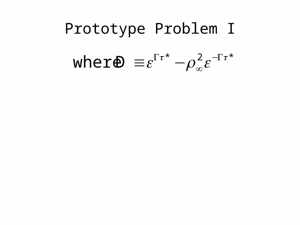
*2* where ττ ρ Γ−∞

Γ −≡ eeD

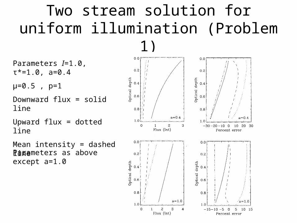
Two stream solution for uniform illumination (Problem 1)

Parameters I=1.0, τ*=1.0, a=0.4

μ=0.5 , p=1

Downward flux = solid line

Upward flux = dotted line

Mean intensity = dashed line

Parameters as above except a=1.0

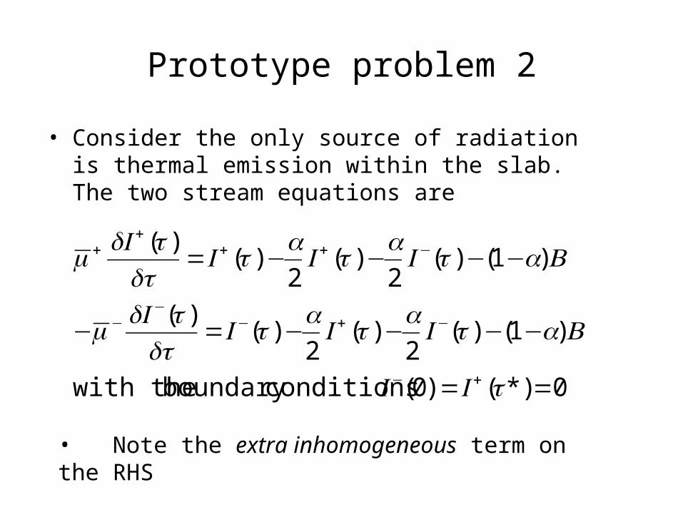
Prototype problem 2

• Consider the only source of radiation is thermal emission within the slab. The two stream equations are

0*)()0( conditionsboundary with the

)1()(2

)(2

)()(

)1()(2

)(2

)()(

==

−−−−=−

−−−−=

+−

−+−−

−

−+++

+

τ

τττττμ

τττττμ

II

BaIa

Ia

Id

dI

BaIa

Ia

Id

dI

• Note the extra inhomogeneous term on the RHS

Prototype problem 2

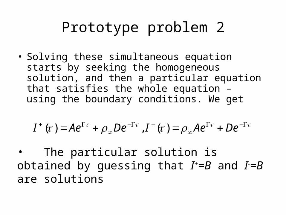
• Solving these simultaneous equation starts by seeking the homogeneous solution, and then a particular equation that satisfies the whole equation – using the boundary conditions. We get

ττττ ρτρτ Γ−Γ∞

−Γ−∞

Γ+ +=+= DeAeIDeAeI )( ,)(

• The particular solution is obtained by guessing that I+=B and I-=B are solutions

Prototype problem 2

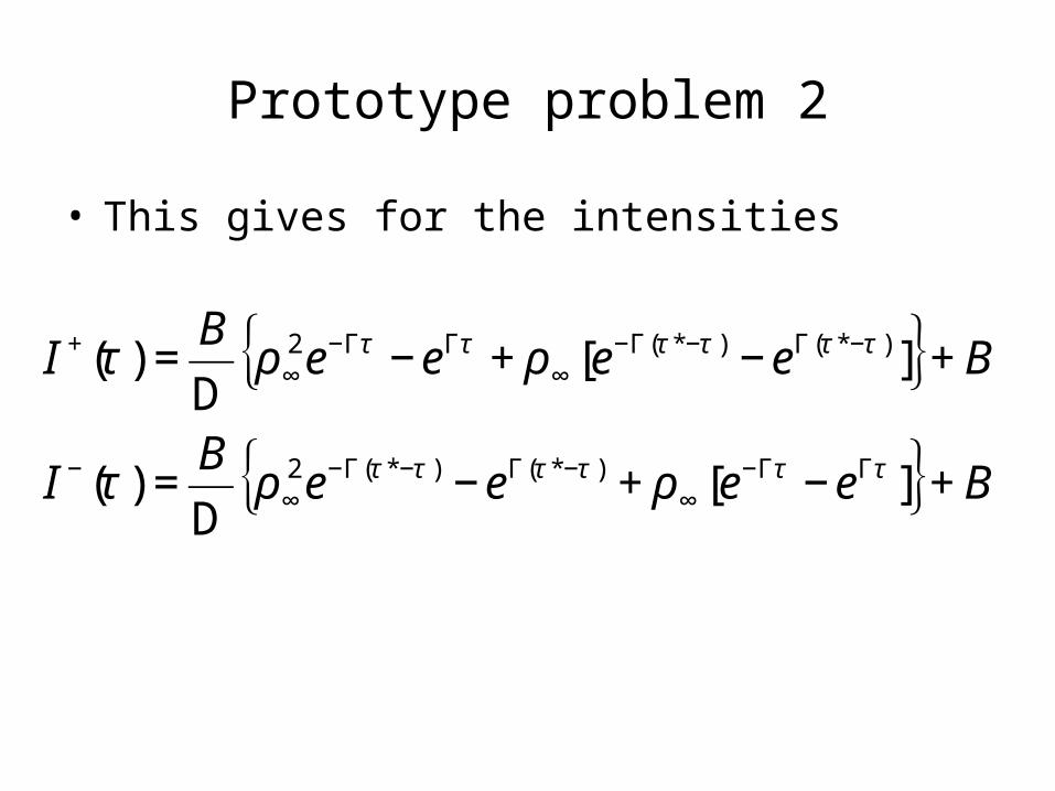
• This gives for the intensities

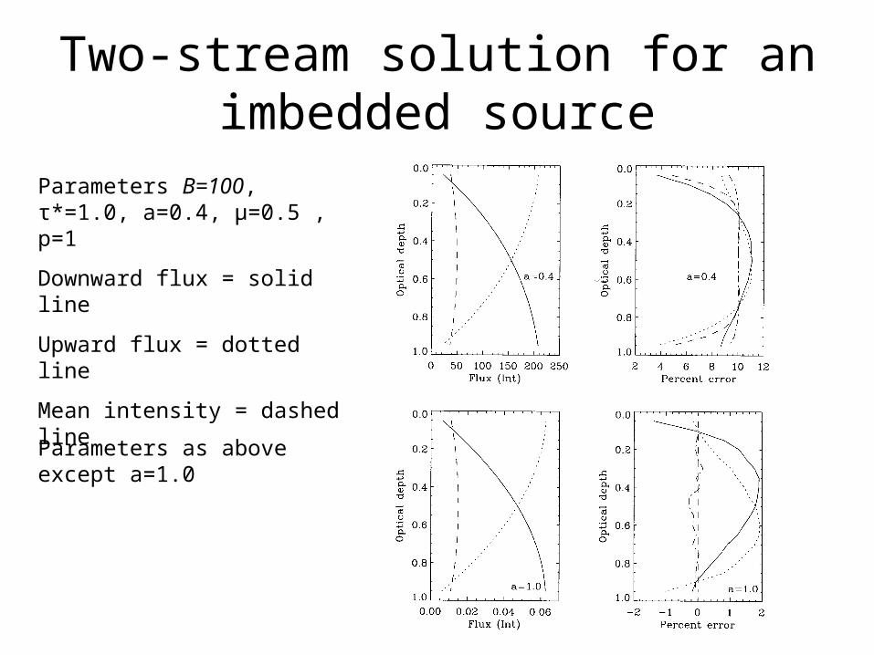
Two-stream solution for an imbedded source

Parameters B=100, τ*=1.0, a=0.4, μ=0.5 , p=1

Downward flux = solid line

Upward flux = dotted line

Mean intensity = dashed line

Parameters as above except a=1.0

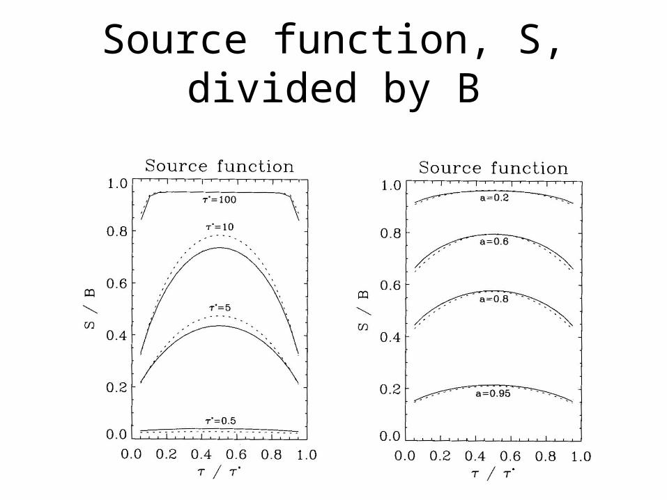
Source function, S, divided by B

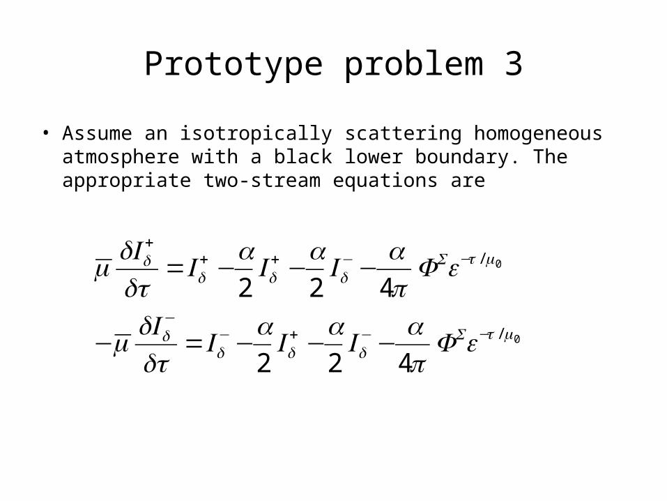
Prototype problem 3

• Assume an isotropically scattering homogeneous atmosphere with a black lower boundary. The appropriate two-stream equations are

0

0

/

/

422

422

μτ

μτ

πτμ

πτμ

−−+−−

−−+++

−−−=−

−−−=

eFa

Ia

Ia

IddI

eFa

Ia

Ia

IddI

Sddd

d

Sddd

d

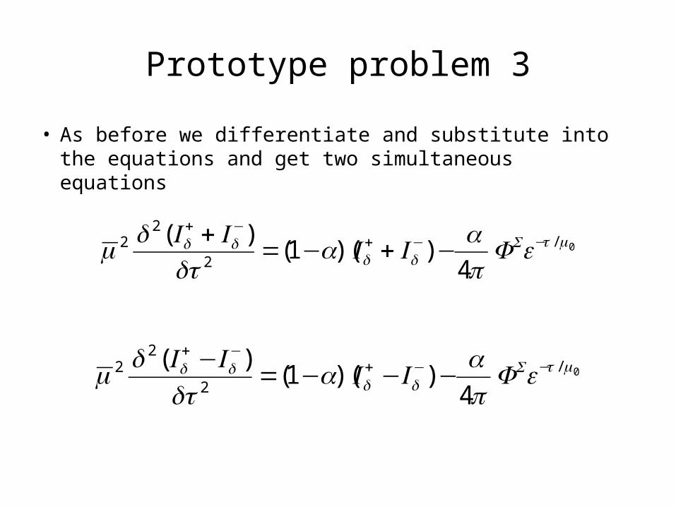
Prototype problem 3

• As before we differentiate and substitute into the equations and get two simultaneous equations

0/2

22

4))(1(

)( μτ

πτμ −−+

−+

−+−=+

eFa

IIad

IId Sdd

dd

0/2

22

4))(1(

)( μτ

πτμ −−+

−+

−−−=−

eFa

IIad

IId Sdd

dd

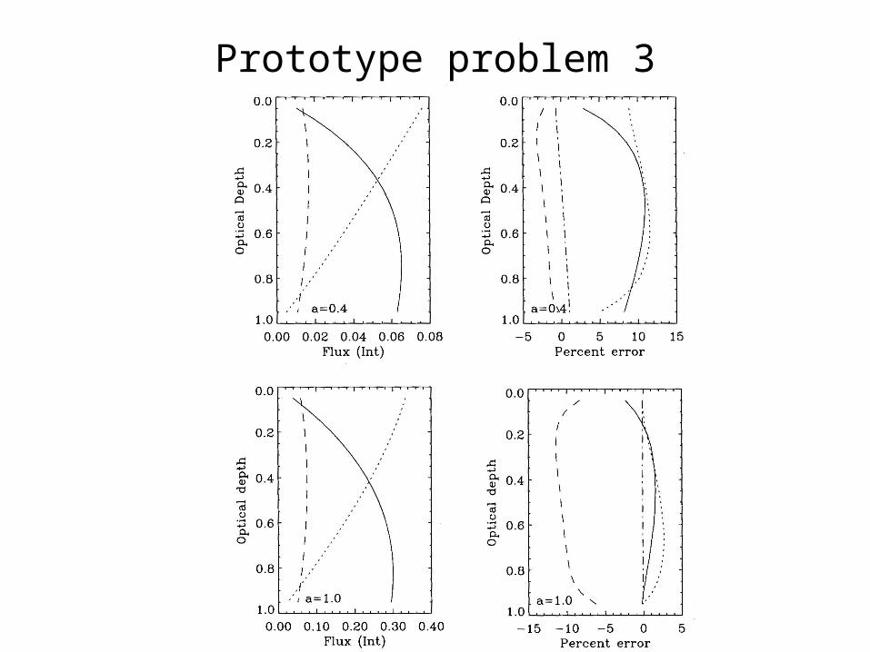
Prototype problem 3

Prototype problem 3

• Using the same solution method as for problem 2 we consider the homogeneous solution

ττττ ρρ Γ−Γ∞

−Γ−∞

Γ+ +=+= DeAeIDeAeI dd ,

• We now guess that a particular solution will be proportional to exp(-τμWe get

0

0

/

/

Z

Z μτττ

μτττ

ρ

ρ−−Γ−Γ

∞−

−+Γ−∞

Γ+

++=

++=

eDeAeI

eDeAeI

d

d

• Z+ and Z- can be determined by substitution

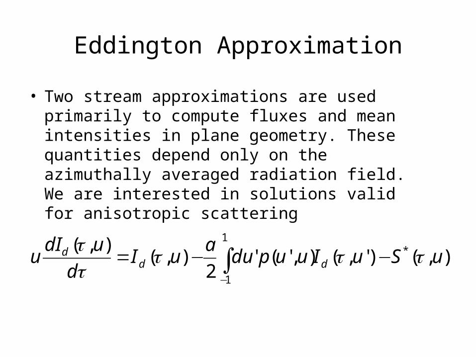
Eddington Approximation

• Two stream approximations are used primarily to compute fluxes and mean intensities in plane geometry. These quantities depend only on the azimuthally averaged radiation field. We are interested in solutions valid for anisotropic scattering

),()',(),'('2

),(),( *

1

1

uSuIuupdua

uId

udIu dd

d τττττ

−−= ∫−

Eddington Approximation

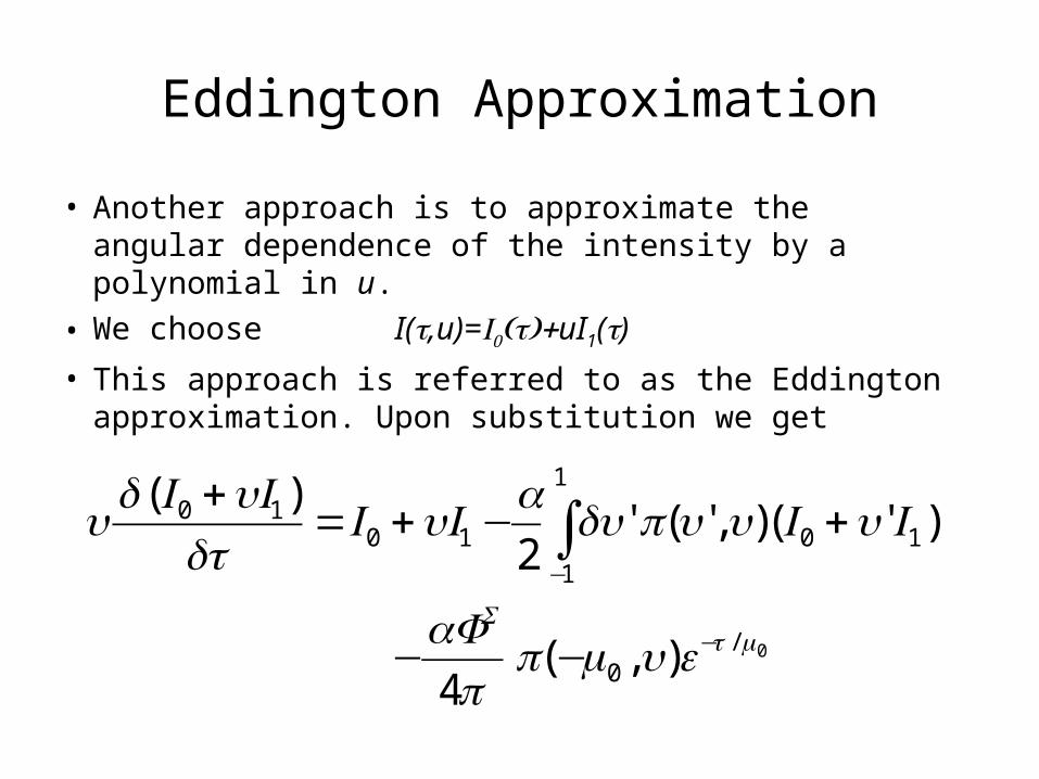
• Another approach is to approximate the angular dependence of the intensity by a polynomial in u.

• We choose I(τ,u)=τ+uI1(τ)

• This approach is referred to as the Eddington approximation. Upon substitution we get

0/0

10

1

1

1010

),(4

)'(),'('2

)(

μτμπ

τ

−

−

−−

+−+=+

∫

eupaF

IuIuupdua

uIIduIId

u

S

Eddington Approximation

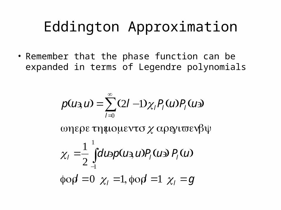
• Remember that the phase function can be expanded in terms of Legendre polynomials

Eddington Approximation

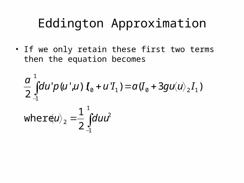
• If we only retain these first two terms then the equation becomes

∫

∫

−

−

=⟩⟨

⟩⟨+=+

1

1

22

1201

1

1

0

2

1 where

)3()')(,'('2

duuu

IuguIaIuIuupdua