1

Chapter 7. XRD (Chapter 8 Campbell & White, Alexander "X-ray Diffraction Methods in Polymer Science").

The general principles of diffraction are covered in Cullity, "Elements of X-ray Diffraction". Ifyou are unfamiliar with XRD you will need to review or read Cullity Chapters 1-7 and theappendices. Alexander's text referenced above is also useful as an introduction to XRD but is lessgeneral and at a slightly more advanced level.

There are a number of differences between x-ray diffraction in polymers and metallurgical (Cullity)or ceramic diffraction.

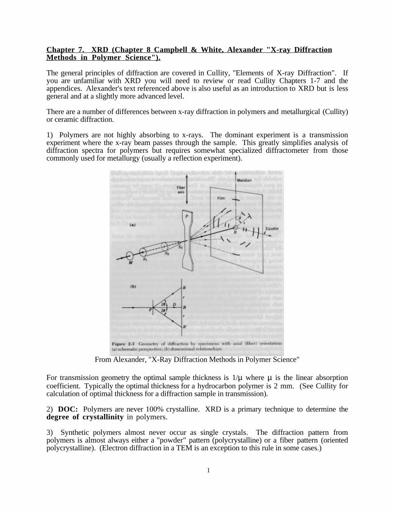
1) Polymers are not highly absorbing to x-rays. The dominant experiment is a transmissionexperiment where the x-ray beam passes through the sample. This greatly simplifies analysis ofdiffraction spectra for polymers but requires somewhat specialized diffractometer from thosecommonly used for metallurgy (usually a reflection experiment).

From Alexander, "X-Ray Diffraction Methods in Polymer Science"

For transmission geometry the optimal sample thickness is 1/µ where µ is the linear absorptioncoefficient. Typically the optimal thickness for a hydrocarbon polymer is 2 mm. (See Cullity forcalculation of optimal thickness for a diffraction sample in transmission).

2) DOC: Polymers are never 100% crystalline. XRD is a primary technique to determine thedegree of crystallinity in polymers.

3) Synthetic polymers almost never occur as single crystals. The diffraction pattern frompolymers is almost always either a "powder" pattern (polycrystalline) or a fiber pattern (orientedpolycrystalline). (Electron diffraction in a TEM is an exception to this rule in some cases.)

2

4) Microstructure: Crystallite size in polymers is usually on the nano-scale in the thicknessdirection. The size of crystallites can be determined using variants of the Scherrer equation.

5) Orientation: Polymers, due to their long chain structure, are highly susceptible toorientation. XRD is a primary tool for the determination of crystalline orientation through theHermans orientation function.

6) Polymer crystals display a relatively large number of defects in some cases. This leads todiffraction peak broadening (see Campbell and White or Alexander for details).

7) Polymer crystallites are very small with a large surface to volume ratio which enhances thecontribution of interfacial disorganization on the diffraction pattern.

8) SAXS: Due to the nano-scale size of polymer crystallites, small-angle scattering isintense in semi-crystalline polymers and a separate field of analysis based on diffraction at anglesbelow 6° has developed (see Alexander and Chapter 8 of these notes for details).

Introduction:

Diffraction or scattering is a separate category of analytic techniques using electromagneticradiation where the interference of radiation arising from structural features is observed. Theinterference pattern is the Fourier transform of the pair wise correlation function. The pairwise correlation function can be constructed in a though experiment where a multiphase material isstatistically described by a line throwing experiment. If lines of length "r" are thrown in to a 2phase material there is a probability that both ends of the lines fall in the dilute phase. Thisprobability in 3-d space changes with the size of the line, "r", and a plot of this probability as afunction of "r" is a plot of the pair wise distribution function. For a crystal the two phases areatoms and voids and peaks in the pair wise correlation function occur at multiples of the latticespacing. Interference which results from correlations of different domains or atoms is usuallyassociated with the "Structure Factor" or "Interference Factor", S2(2θ). Interference can also occurif the individual domains are prefect structures such as spheres. For a sphere, there is a sharpdecay in the pair wise correlation function near the diameter of the sphere and this sharp decayresults in a peak in the Fourier transform of the correlation function. For a metal crystal thiscorresponds to the atomic form factor, f2(2θ). For larger scale domains interference associated

with the form of the scattering units is generally termed the "form factor", F2(2θ).

The scattered intensity as a function of angle is then the product of two terms, the form factor(f2(2θ) or F2(2θ)) and the structure factor (S2 (2θ)):

I(2θ) = Constant F2(2θ) S2 (2θ)

For XRD the form factor is usually obtained from tabulated values and the major interest is in theStructure factor. For small angle scattering dilute conditions are usually of interest making thestructure factor go to a constant value of 1 and the form factor for complex structures areinvestigated.

Thus, the basic principles of scattering and diffraction are the same, while the implementation ofthese principles are quite different.

Bragg's Law:

3

Cullity and Alexander derive Bragg's Law using the mirror analogy (specular analogy). It can alsobe derived from interference laws or using "inverse space" (see appendix in Cullity). The featuresof Bragg's Law is that structural size is inversely proportional to a reduced scattering angle, sohigh angle relates to smaller structure and low angle relates to large structure. Small-anglescattering measures colloidal to nano-scale sizes. There is no large scale limit to diffraction. Thesmall scale limit (i.e. the smallest measurable size) is λ/2 as is inherent in Bragg's Law:

d = λ/2 (1/sinθ)

θ is half of the scattering angle measured from the incident beam. The 1/sinθ term in Bragg's law

acts as an amplification factor. The minimum value of which is 1 for 2θ = 180° (direct backscattering). The maximum value of the amplification factor is ∞ so that theoretically no size limitexists with a given radiation of wave length λ . In reality the diffraction geometry and coherencelength of the radiation leads to a large scale limit on the micron scale.

Typically diffracted intensity if plotted as a function of 2θ. Since the d-spacing is of interest one

might wonder why diffraction data isn't plotted as a function of sinθ or 1/sinθ. This is in fact

done with the use of the "scattering vector" q or s. q = 4π/λ sin(θ) = 2π/d and s = 2/λ sin(θ) =1/d. The appendix of Cullity gives a good description of diffraction in "q" or "s" reciprocal space.

The Fourier transform of the real space vector, "r", used to determine the pair wise correlationfunction is the scattering vector "q".

Review of Crystalline Polymer Morphology:

"Molecular" scale Crystalline Structure:

Consider that we can form an all-trans oligmeric polyethylene sample an bring it below thecrystallization temperature. The molecules will be in the minimum energy state and will bein a planar zigzag form. These molecular sheets, when viewed from end will look like aline just as viewing a rigid strip from the end will appear as a line.

Crystal systems are described by lattice parameters (for review see Cullity X-ray Diffraction forinstance). A unit cell consists of three size parameters, a,b,c and three angles α, β, γ.Cells are categorized into 14 Bravis Lattices which can be categorized by symmetry forinstance. All unit cells fall into one of the Bravis Lattices. Typically, simple molecules andatoms form highly symmetric unit cells such as simple cubic (a=b=c, α=β=γ=90°) orvariants such as Face Center Cubic or Body Centered Cubic. The highest density crystal isformed equivalently by FCC and Hexagonal Closest Packed (HCP) crystal structures.These are the crystal structures chosen by extremely simple systems such as colloidalcrystals. Also, Proteins will usually crystallize into one of these closest packed forms.This is because the collapsed protein structure (the whole protein) crystallizes as a unit celllattice site. In some cases it is possible to manipulate protein molecules to crystallize inlamellar crystals but this is extremely difficult.

As the unit cell lattice site becomes more complicated and/or becomes capable of bonding indifferent ways in different directions the Bravis lattice becomes more complicated, i.e. lesssymmetric. This is true for oligomeric organic molecules. For example olefins (such asdodecane (n=12) and squalene (n=112)) crystallize into an orthorhombic unit cells which

4

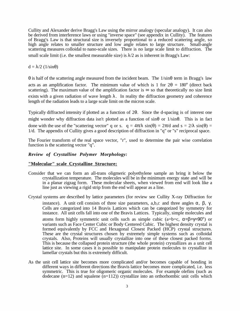
have a, b and c different while α=β=γ=90°. The reason a, b and c are different is thedifferent bonding mechanisms in the different directions. This is reflected in vastlydifferent thermal expansion coefficients in the different directions. The orthorhombicstructure of olefinic crystals is shown below. Two chains make up the unit cell lattice site(shown in bold). The direction of the planar zigzag (or helix) in a polymer crystal isalways the c-axis by convention.

a

bc

PE/Olefin crystal structure.

See also, Campbell and White figure 8.4. Chain Folding:

The planar zigzag of the olefin or PE molecule crystallize as shown above into an orthogonal unitcell. This unit cell can be termed the first or primary level of structure for the olefin crystal.Consider a metal crystal such as the FCC structure of copper. The copper atoms diffuse tothe closest packed crystal planes and the crystal grows in 3-dimensions along low-indexcrystal faces until some kinetic feature interferes with growth. In a pure melt with lowthermal quench and careful control over the growth front through removal of the growingcrystal from the melt, a single crystal can be formed. Generally, for a metal crystal there isno particular limitation which would lead to asymmetric growth of the crystallite and fairlysymmetric crystals result.

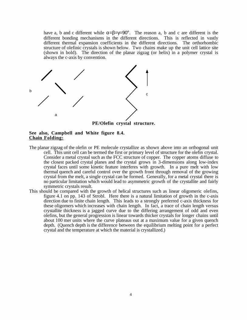
This should be compared with the growth of helical structures such as linear oligomeric olefins,figure 4.1 on pp. 143 of Strobl. Here there is a natural limitation of growth in the c-axisdirection due to finite chain length. This leads to a strongly preferred c-axis thickness forthese oligomers which increases with chain length. In fact, a trace of chain length versuscrystallite thickness is a jagged curve due to the differing arrangement of odd and evenolefins, but the general progression is linear towards thicker crystals for longer chains untilabout 100 mer units where the curve plateaus out at a maximum value for a given quenchdepth. (Quench depth is the difference between the equilibrium melting point for a perfectcrystal and the temperature at which the material is crystallized.)

5

Number of mer units

Cry

stal

lite

Thi

ckn

ess Depends on

Quench Depth∆T

Schematic of olefin crystallite thickness as a function of the chain length.

The point in the curve where the crystallite thickness reaches a plateau value in molecular weight isclose to the molecular weight where chains begin to entangle with each other in the melt andthere is some association between these two phenomena. Also, the fact that this plateauthickness has a strong inverse quench depth dependence suggests that there is someentropic feature to this behavior (pp. 163 eqn. 4.20 where dc is the crystallite thickness andpp. 164 figure 4.18 Strobl).

Considering a random model for chain structure such as shown in figure 2.5 on pp. 21 as well asthe rotational isomeric state model for formation of the planar zigzag structure in PE, pp. 15figure 2.2, it should be clear that entropy favors some bending of the rigid linear structure,and that this is allowed, with some energy penalty associated with gauche conformation offigure 2.2. Put another way, for chains of a certain length (Close to the entanglementmolecular weight) there is a high-statistical probability that the chains will bend even belowthe crystallization temperature where the planar zigzag conformation is preferred for PE.When chains bend there is a local free energy penalty which must be paid and this can beincluded in a free energy balance in terms of a fold-surface energy if it is considered thatthese bends are locally confined to the crystallite surface as shown on pp. 161 figure 4.15;and pp. 185 figure 4.34.

There are many different crystalline structures which can be formed under different processingconditions for semi-crystalline polymers (Figures 4.2- 4.7 pp. 145 to 149; figure 4.13 pp.157; Figure 4.19, pp. 165; figure 4.21 pp. 170). As a class these variable crystallineforms have only two universal characteristics:

1) Unit cell structure as discussed above.2) Relationship between lamellar thickness and quench depth.

This means that understanding the relationship between quench depth and crystallite thickness isone of only two concrete features for polymer crystals. John Hoffman was the first todescribe this relationship although his derivation of a crystallite thickness law borrowedheavily on asymmetric growth models form low molecular weight, particularly ceramic anmetallurgical systems. Hoffman's law is given in equation 4.23 on pp. 166:

nT

H T Tm e f

mf

f

* ,=−( )∞

∞

2σ∆

, Hoffman Law

6

where n* is the thickness of the equilibrium crystal crystallized at T (which is below theequilibrium melting point for a crystal of infinite thickness, Tf

∞), σ is the excess surface

free energy associated with folded chains at the lateral surface of platelet crystals, and ∆His the heat of fusion associated with one monomer.

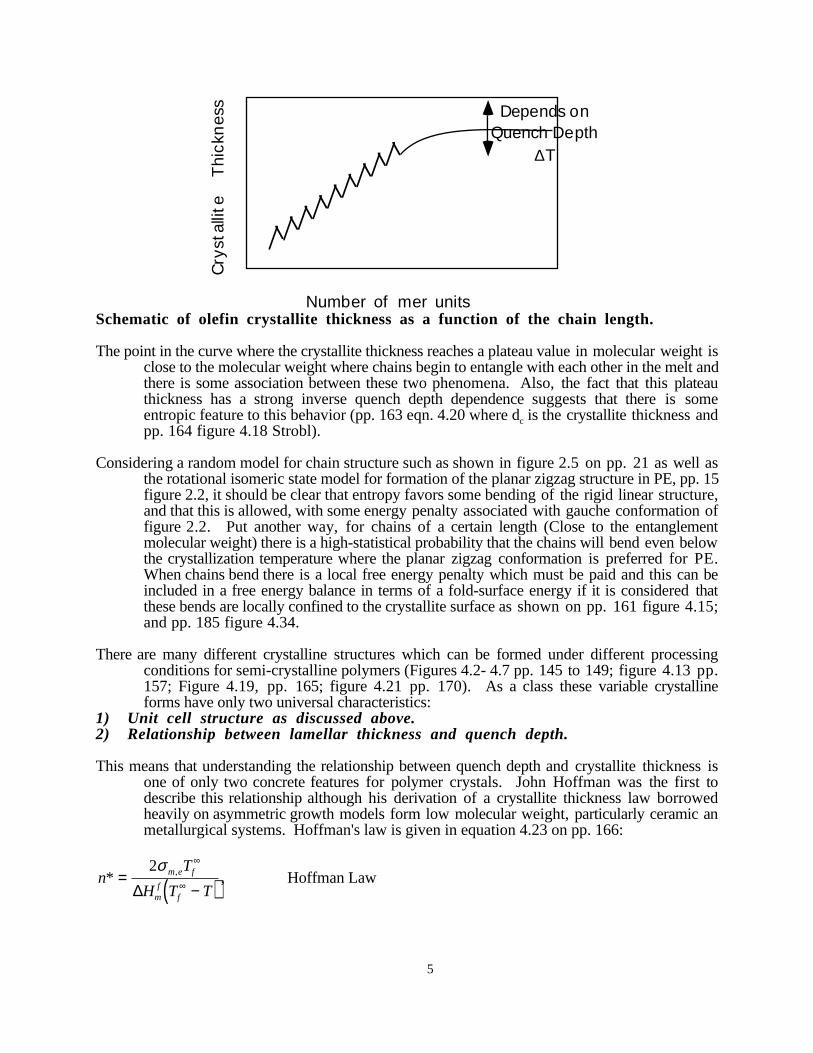
Hoffman's law can be obtained very quickly for a free energy balance following the "Gibbs-Thomson Approach" (Strobl pp. 166) if on considers that the crystals will formasymmetrically due to entropically required chain folds and that the surface energy for thefold surface is much higher than that for the c-axis sides..

σ

R

t

At the equilibrium melting point ∆G∞ = 0 = ∆H - T∞ ∆S, so ∆S = ∆H/ T∞. At some temperature, T, below the equilibrium melting point, The volumetric change in free energy

for crystallization ∆fT = ∆H - T ∆S = ∆H(1 - T/T∞) = ∆H(T∞ - T)/ T∞.

The crystallite crystallized at "T" is in equilibrium with its melt and this equilibrium state is adjustedby adjusting the thickness of the crystallite using the surface energy, that is,

∆GT = 4Rt σside+ 2R2 σ - R2t ∆fT = 0 at T. That is, At T the crystallite of thickness "t" is in equilibrium with its melt and this equilibrium is

determined by the asymmetry of the crystallite, t/R. If ∆fT = ∆H(T∞ - T)/ T∞. is use in thisexpression,

4t σside+ 2R σ = R t ∆H(T∞ - T)/ T∞.

Assuming that σside <<< σ, and "t"<<<"R" then,

t = 2 σ T∞./( ∆H(T∞ - T))which is the Hoffman law.

The deeper the quench, (T∞ - T), the thinner the crystal and for a crystal crystallized at T∞, thecrystallite is of infinite thickness. (Crystallization does not occur at T∞).

Nature of the Chain Fold Surface:

In addition to determination of T∞, the specific nature of the lamellar interface in terms of molecularconformation is of critical importance to the Hoffman analysis. There are several limitingexamples, 1) Regular Adjacent Reentry, 2) Switchboard Model (Non-Adjacent

7

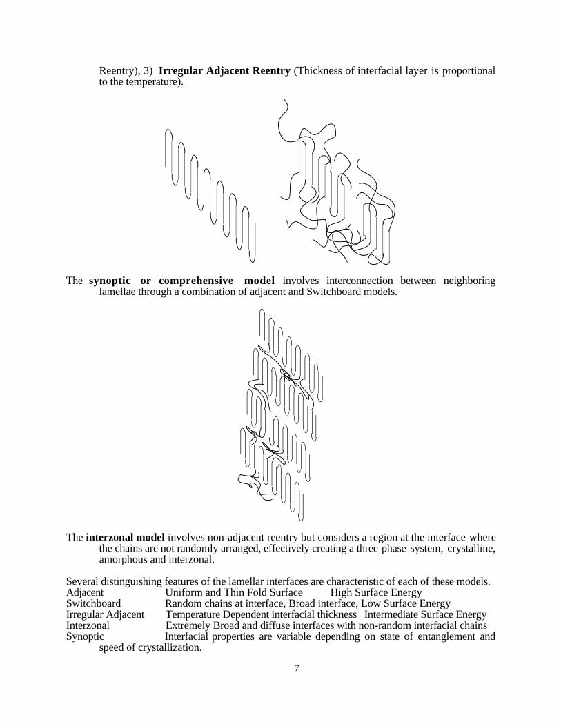
Reentry), 3) Irregular Adjacent Reentry (Thickness of interfacial layer is proportionalto the temperature).

The synoptic or comprehensive model involves interconnection between neighboringlamellae through a combination of adjacent and Switchboard models.

The interzonal model involves non-adjacent reentry but considers a region at the interface wherethe chains are not randomly arranged, effectively creating a three phase system, crystalline,amorphous and interzonal.

Several distinguishing features of the lamellar interfaces are characteristic of each of these models.Adjacent Uniform and Thin Fold Surface High Surface EnergySwitchboard Random chains at interface, Broad interface, Low Surface EnergyIrregular Adjacent Temperature Dependent interfacial thickness Intermediate Surface EnergyInterzonal Extremely Broad and diffuse interfaces with non-random interfacial chainsSynoptic Interfacial properties are variable depending on state of entanglement and

speed of crystallization.

8

The Hoffman equation states that the lamellar thickness is proportional to the interfacial energy sowe can say that Adjacent reentry favors thicker lamellae since adjacent reentry has thehighest interfacial energy and the more random interfacial regions should display thinnerlamellae.

Colloidal Scale Structure in Semi-Crystalline Polymers:

Lamellae crystallized in dilute solution by precipitation can form pyramid shaped crystallites whichare essentially single lamellar crystals (figure 4.21 for example). Pyramids form due tochain tilt in the lamellae which leads to a strained crystal if growth proceeds in 2dimensions only. In some cases these lamellae (which have an aspect ratio similar to asheet of paper) can stack although this is usually a weak feature in solution crystallizedpolymers.

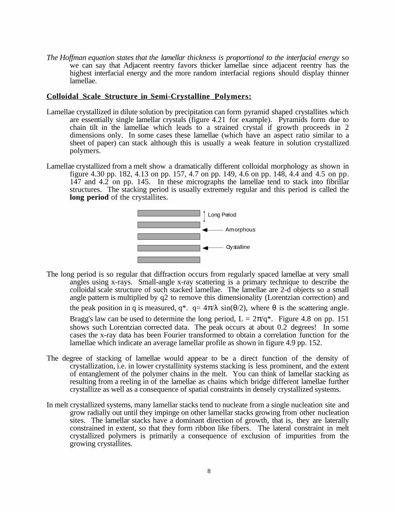
Lamellae crystallized from a melt show a dramatically different colloidal morphology as shown infigure 4.30 pp. 182, 4.13 on pp. 157, 4.7 on pp. 149, 4.6 on pp. 148, 4.4 and 4.5 on pp.147 and 4.2 on pp. 145. In these micrographs the lamellae tend to stack into fibrillarstructures. The stacking period is usually extremely regular and this period is called thelong period of the crystallites.

Long Period

Amorphous

Crystalline

The long period is so regular that diffraction occurs from regularly spaced lamellae at very smallangles using x-rays. Small-angle x-ray scattering is a primary technique to describe thecolloidal scale structure of such stacked lamellae. The lamellae are 2-d objects so a smallangle pattern is multiplied by q2 to remove this dimensionality (Lorentzian correction) andthe peak position in q is measured, q*. q= 4π/λ sin(θ/2), where θ is the scattering angle.

Bragg's law can be used to determine the long period, L = 2π/q*. Figure 4.8 on pp. 151shows such Lorentzian corrected data. The peak occurs at about 0.2 degrees! In somecases the x-ray data has been Fourier transformed to obtain a correlation function for thelamellae which indicate an average lamellar profile as shown in figure 4.9 pp. 152.

The degree of stacking of lamellae would appear to be a direct function of the density ofcrystallization, i.e. in lower crystallinity systems stacking is less prominent, and the extentof entanglement of the polymer chains in the melt. You can think of lamellar stacking asresulting from a reeling in of the lamellae as chains which bridge different lamellae furthercrystallize as well as a consequence of spatial constraints in densely crystallized systems.

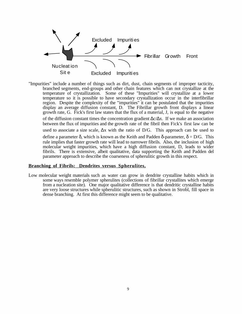
In melt crystallized systems, many lamellar stacks tend to nucleate from a single nucleation site andgrow radially out until they impinge on other lamellar stacks growing from other nucleationsites. The lamellar stacks have a dominant direction of growth, that is, they are laterallyconstrained in extent, so that they form ribbon like fibers. The lateral constraint in meltcrystallized polymers is primarily a consequence of exclusion of impurities from thegrowing crystallites.

9

Fibrillar Growth Front

Excluded Impuriti es

Excluded Impuriti esNucleat ion

Sit e

"Impurities" include a number of things such as dirt, dust, chain segments of improper tacticity,branched segments, end-groups and other chain features which can not crystallize at thetemperature of crystallization. Some of these "Impurities" will crystallize at a lowertemperature so it is possible to have secondary crystallization occur in the interfibrillarregion. Despite the complexity of the "impurities" it can be postulated that the impuritiesdisplay an average diffusion constant, D. The Fibrillar growth front displays a lineargrowth rate, G. Fick's first law states that the flux of a material, J, is equal to the negativeof the diffusion constant times the concentration gradient ∆c/∆x. If we make an associationbetween the flux of impurities and the growth rate of the fibril then Fick's first law can beused to associate a size scale, ∆x with the ratio of D/G. This approach can be used to

define a parameter δ, which is known as the Keith and Padden δ-parameter, δ = D/G. Thisrule implies that faster growth rate will lead to narrower fibrils. Also, the inclusion of highmolecular weight impurities, which have a high diffusion constant, D, leads to widerfibrils. There is extensive, albeit qualitative, data supporting the Keith and Padden delparameter approach to describe the coarseness of spherulitic growth in this respect.

Branching of Fibrils: Dendrites versus Spherulites.

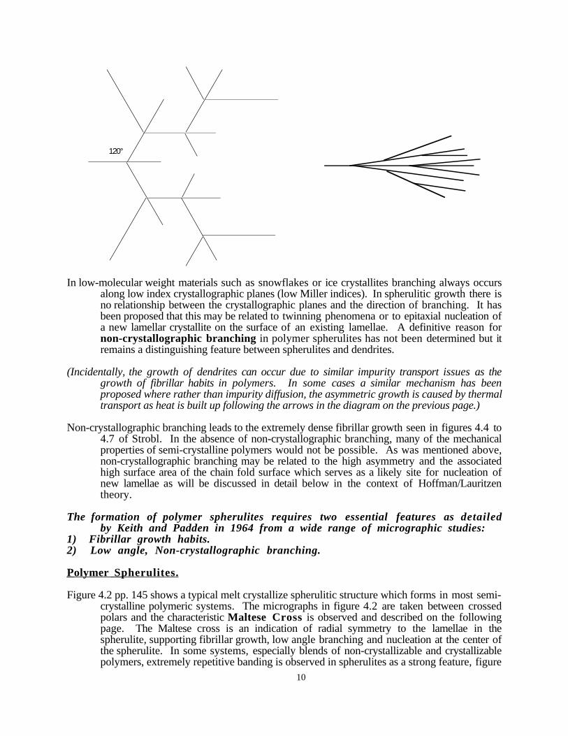
Low molecular weight materials such as water can grow in dendrite crystalline habits which insome ways resemble polymer spherulites (collections of fibrillar crystallites which emergefrom a nucleation site). One major qualitative difference is that dendritic crystalline habitsare very loose structures while spherulitic structures, such as shown in Strobl, fill space indense branching. At first this difference might seem to be qualitative.

10

120°

In low-molecular weight materials such as snowflakes or ice crystallites branching always occursalong low index crystallographic planes (low Miller indices). In spherulitic growth there isno relationship between the crystallographic planes and the direction of branching. It hasbeen proposed that this may be related to twinning phenomena or to epitaxial nucleation ofa new lamellar crystallite on the surface of an existing lamellae. A definitive reason fornon-crystallographic branching in polymer spherulites has not been determined but itremains a distinguishing feature between spherulites and dendrites.

(Incidentally, the growth of dendrites can occur due to similar impurity transport issues as thegrowth of fibrillar habits in polymers. In some cases a similar mechanism has beenproposed where rather than impurity diffusion, the asymmetric growth is caused by thermaltransport as heat is built up following the arrows in the diagram on the previous page.)

Non-crystallographic branching leads to the extremely dense fibrillar growth seen in figures 4.4 to4.7 of Strobl. In the absence of non-crystallographic branching, many of the mechanicalproperties of semi-crystalline polymers would not be possible. As was mentioned above,non-crystallographic branching may be related to the high asymmetry and the associatedhigh surface area of the chain fold surface which serves as a likely site for nucleation ofnew lamellae as will be discussed in detail below in the context of Hoffman/Lauritzentheory.

The formation of polymer spherulites requires two essential features as detailedby Keith and Padden in 1964 from a wide range of micrographic studies:

1) Fibrillar growth habits.2) Low angle, Non-crystallographic branching.

Polymer Spherulites.

Figure 4.2 pp. 145 shows a typical melt crystallize spherulitic structure which forms in most semi-crystalline polymeric systems. The micrographs in figure 4.2 are taken between crossedpolars and the characteristic Maltese Cross is observed and described on the followingpage. The Maltese cross is an indication of radial symmetry to the lamellae in thespherulite, supporting fibrillar growth, low angle branching and nucleation at the center ofthe spherulite. In some systems, especially blends of non-crystallizable and crystallizablepolymers, extremely repetitive banding is observed in spherulites as a strong feature, figure

11

4.7 pp. 149. Banding is especially prominent in tactic/atactic blends of polyesters and it isin these systems in which it has been most studied. It has been proposed by Keith thatbanding is related to regular twisting of lamellar bundles in the spherulite (circa 1980).Keith has proposed that this twisting is induced by surface tension in the fold surfacecaused by chain tilt in the lamellae (circa 1989). Since most spherulites crystallize in anextremely dense manner it has been difficult to support Keith's hypothesis withexperimental data. Regular banding has, apparently, no consequences for the mechanicalproperties of semi-crystalline polymers so has been essentially ignored in recent literature.

XRD of Polymers:Four main features of XRD are of importance to Polymer Analysis:

1) Indexing of Crystal Structures2) Microstructure3) Degree of Crystallinity4) Orientation

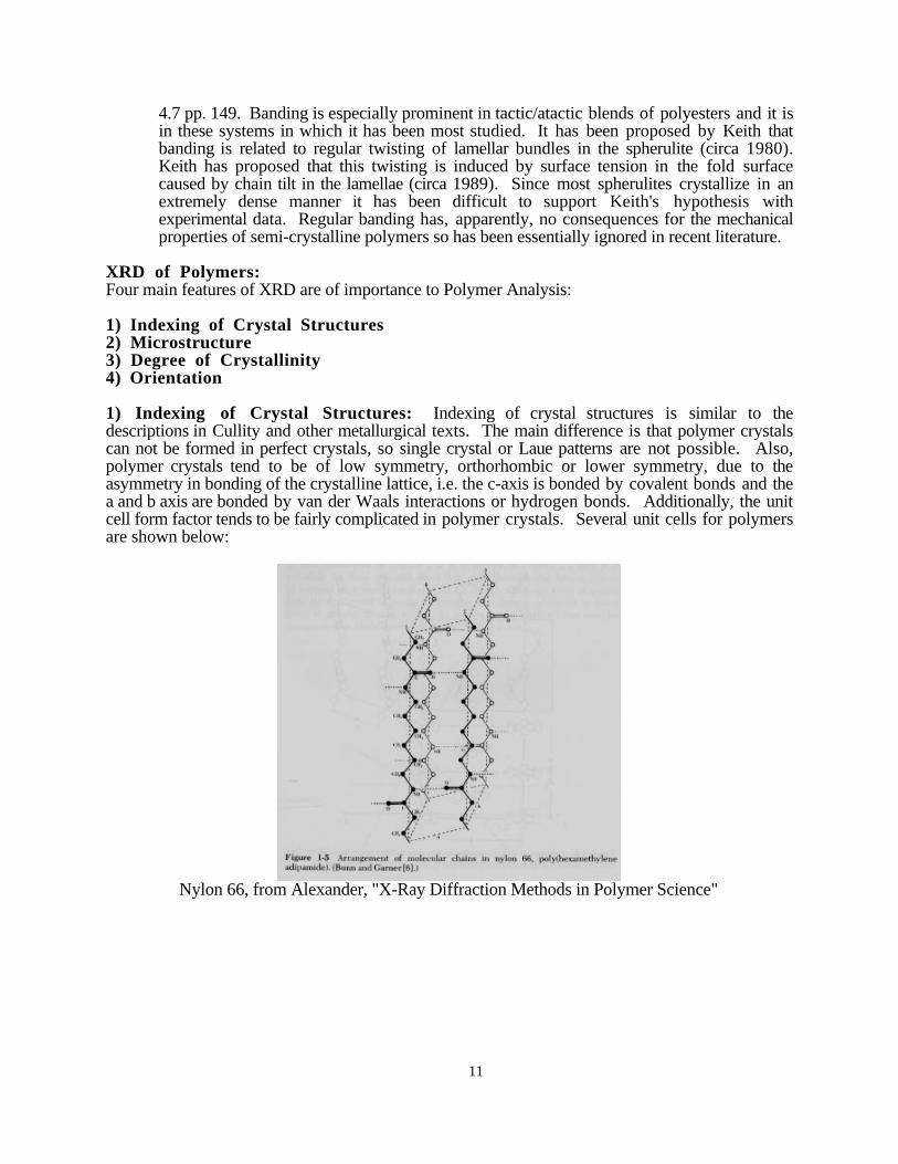
1) Indexing of Crystal Structures: Indexing of crystal structures is similar to thedescriptions in Cullity and other metallurgical texts. The main difference is that polymer crystalscan not be formed in perfect crystals, so single crystal or Laue patterns are not possible. Also,polymer crystals tend to be of low symmetry, orthorhombic or lower symmetry, due to theasymmetry in bonding of the crystalline lattice, i.e. the c-axis is bonded by covalent bonds and thea and b axis are bonded by van der Waals interactions or hydrogen bonds. Additionally, the unitcell form factor tends to be fairly complicated in polymer crystals. Several unit cells for polymersare shown below:

Nylon 66, from Alexander, "X-Ray Diffraction Methods in Polymer Science"

12

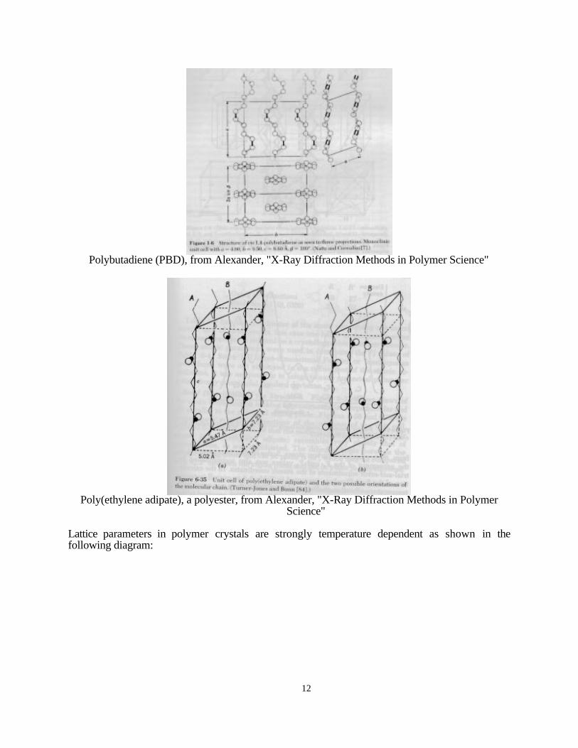
Polybutadiene (PBD), from Alexander, "X-Ray Diffraction Methods in Polymer Science"

Poly(ethylene adipate), a polyester, from Alexander, "X-Ray Diffraction Methods in PolymerScience"

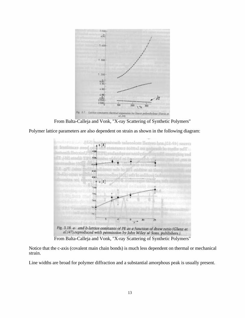
Lattice parameters in polymer crystals are strongly temperature dependent as shown in thefollowing diagram:

13

From Balta-Calleja and Vonk, "X-ray Scattering of Synthetic Polymers"

Polymer lattice parameters are also dependent on strain as shown in the following diagram:

From Balta-Calleja and Vonk, "X-ray Scattering of Synthetic Polymers"

Notice that the c-axis (covalent main chain bonds) is much less dependent on thermal or mechanicalstrain.

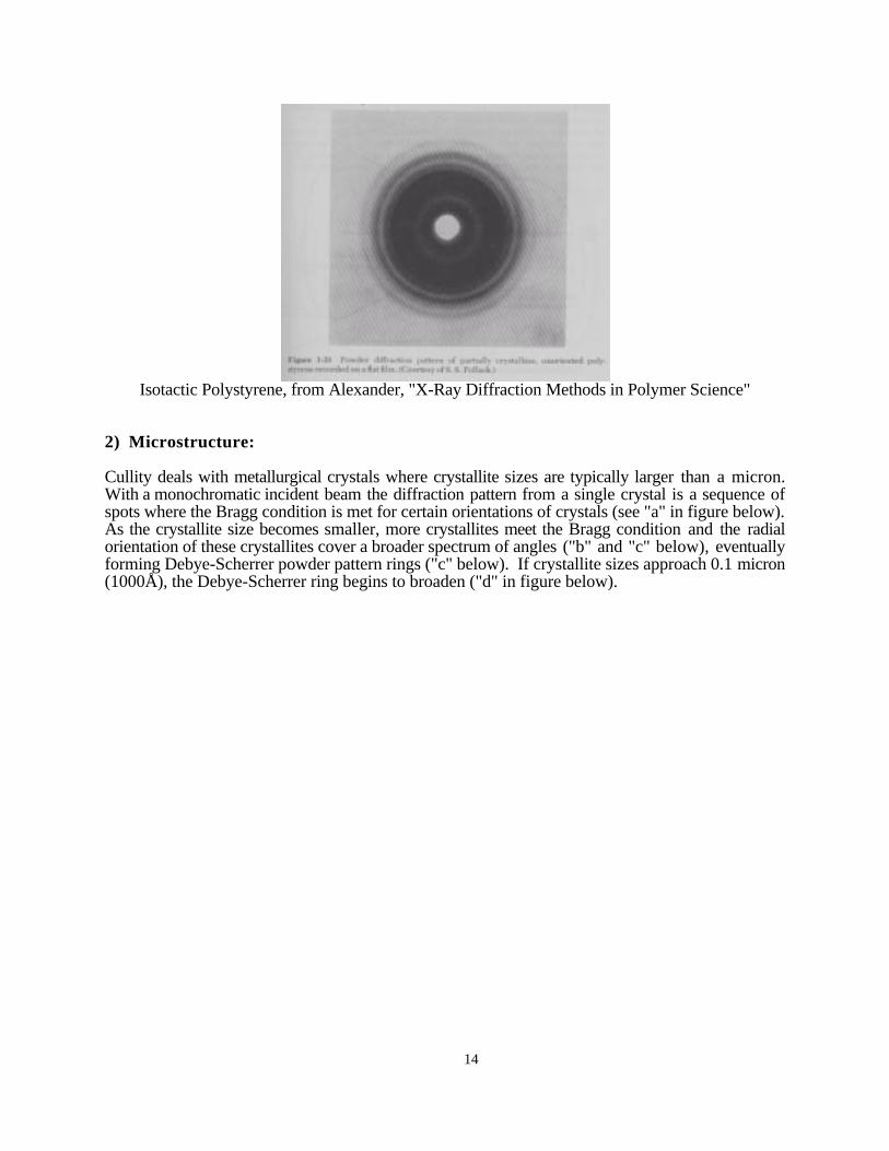
Line widths are broad for polymer diffraction and a substantial amorphous peak is usually present.

14

Isotactic Polystyrene, from Alexander, "X-Ray Diffraction Methods in Polymer Science"

2) Microstructure:

Cullity deals with metallurgical crystals where crystallite sizes are typically larger than a micron.With a monochromatic incident beam the diffraction pattern from a single crystal is a sequence ofspots where the Bragg condition is met for certain orientations of crystals (see "a" in figure below).As the crystallite size becomes smaller, more crystallites meet the Bragg condition and the radialorientation of these crystallites cover a broader spectrum of angles ("b" and "c" below), eventuallyforming Debye-Scherrer powder pattern rings ("c" below). If crystallite sizes approach 0.1 micron(1000Å), the Debye-Scherrer ring begins to broaden ("d" in figure below).

15

From Cullity, "Elements of X-Ray Diffraction

Polymer crystals are on the order of 100Å in thickness. Broadening of the diffraction lines due tosmall crystallite size becomes a dominant effect and the breadth of the diffraction lines can be usedto measure the thickness of lamellar crystals using the Scherrer equation:

tB

=( )

0 9.

cos

λθ

λ is the x-ray wavelength, B is the half width at half height for the diffraction peak in radians and θis half of the diffraction angle. The Scherrer equation is derived in Cullity and other texts. Use ofthe Scherrer equation is a primary technique to determine lamellar thickness in polymer crystallites.This can be used in conjunction with the Hoffman-Lauritzen (Gibbs-Thompson) equation forstudies of crystallization.

In addition to Scherrer broadening diffraction lines can be broadened in polymers due to defects inthe structure. This will not be covered in detail in this course but is described in Campbell andWhite and in Alexander's text.

3) Degree of Crystallinity:

Polymers are never 100% crystalline since the stereochemistry is never perfect, chains containdefects such as branches, and crystallization is highly rate dependent in polymers due to the highviscosity and low transport rates in polymer melts. A primary use of XRD in polymers is

16

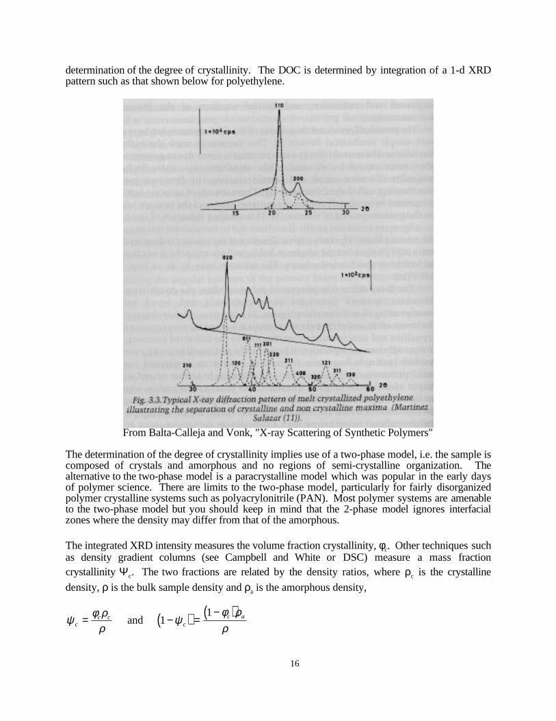
determination of the degree of crystallinity. The DOC is determined by integration of a 1-d XRDpattern such as that shown below for polyethylene.

From Balta-Calleja and Vonk, "X-ray Scattering of Synthetic Polymers"

The determination of the degree of crystallinity implies use of a two-phase model, i.e. the sample iscomposed of crystals and amorphous and no regions of semi-crystalline organization. Thealternative to the two-phase model is a paracrystalline model which was popular in the early daysof polymer science. There are limits to the two-phase model, particularly for fairly disorganizedpolymer crystalline systems such as polyacrylonitrile (PAN). Most polymer systems are amenableto the two-phase model but you should keep in mind that the 2-phase model ignores interfacialzones where the density may differ from that of the amorphous.

The integrated XRD intensity measures the volume fraction crystallinity, φc. Other techniques suchas density gradient columns (see Campbell and White or DSC) measure a mass fractioncrystallinity Ψc. The two fractions are related by the density ratios, where ρc is the crystalline

density, ρ is the bulk sample density and ρa is the amorphous density,

ψ φ ρρ

ψφ ρρc

c cc

c a= −( ) =−( )

and 11

17

If the density of the sample is known from a density gradient column, the weight fraction degree ofcrystallinity can be obtained using:

ψ ρρ

ρ ρρ ρc

c a

c a

= −−

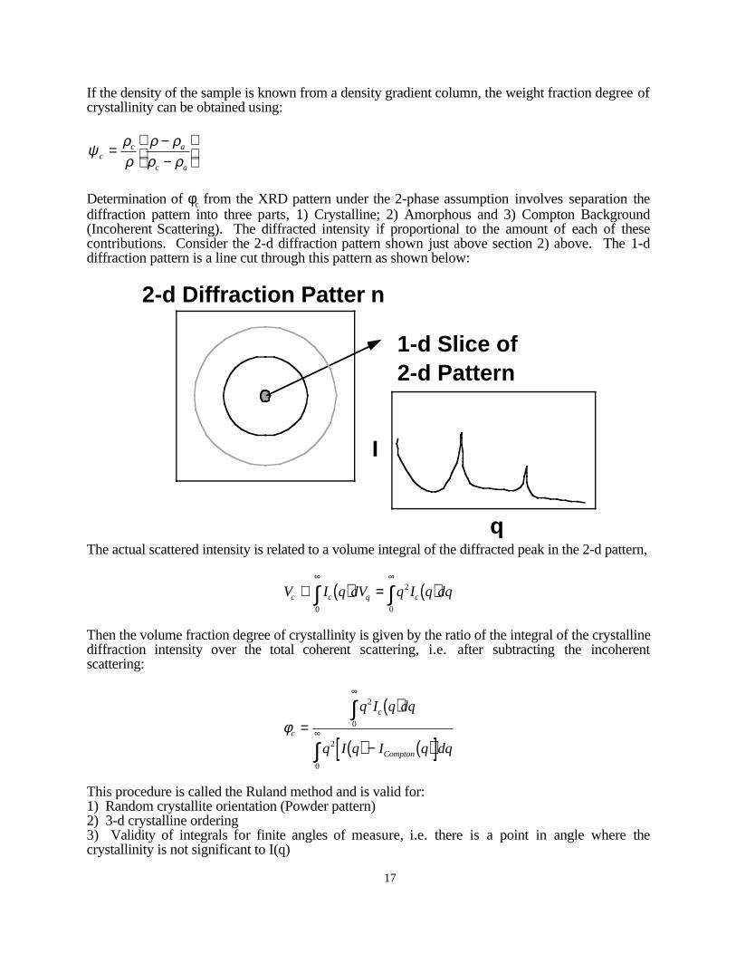
Determination of φc from the XRD pattern under the 2-phase assumption involves separation thediffraction pattern into three parts, 1) Crystalline; 2) Amorphous and 3) Compton Background(Incoherent Scattering). The diffracted intensity if proportional to the amount of each of thesecontributions. Consider the 2-d diffraction pattern shown just above section 2) above. The 1-ddiffraction pattern is a line cut through this pattern as shown below:

1-d Slice of2-d Pattern

2-d Diffraction Patter n

q

I

The actual scattered intensity is related to a volume integral of the diffracted peak in the 2-d pattern,

V I q dV q I q dqc c q c∝ ( ) = ( )∞ ∞

∫ ∫0

2

0

Then the volume fraction degree of crystallinity is given by the ratio of the integral of the crystallinediffraction intensity over the total coherent scattering, i.e. after subtracting the incoherentscattering:

φc

c

Compton

q I q dq

q I q I q dq

=( )

( ) − ( )[ ]

∞

∞

∫

∫

2

0

2

0

This procedure is called the Ruland method and is valid for:1) Random crystallite orientation (Powder pattern)2) 3-d crystalline ordering3) Validity of integrals for finite angles of measure, i.e. there is a point in angle where thecrystallinity is not significant to I(q)

18

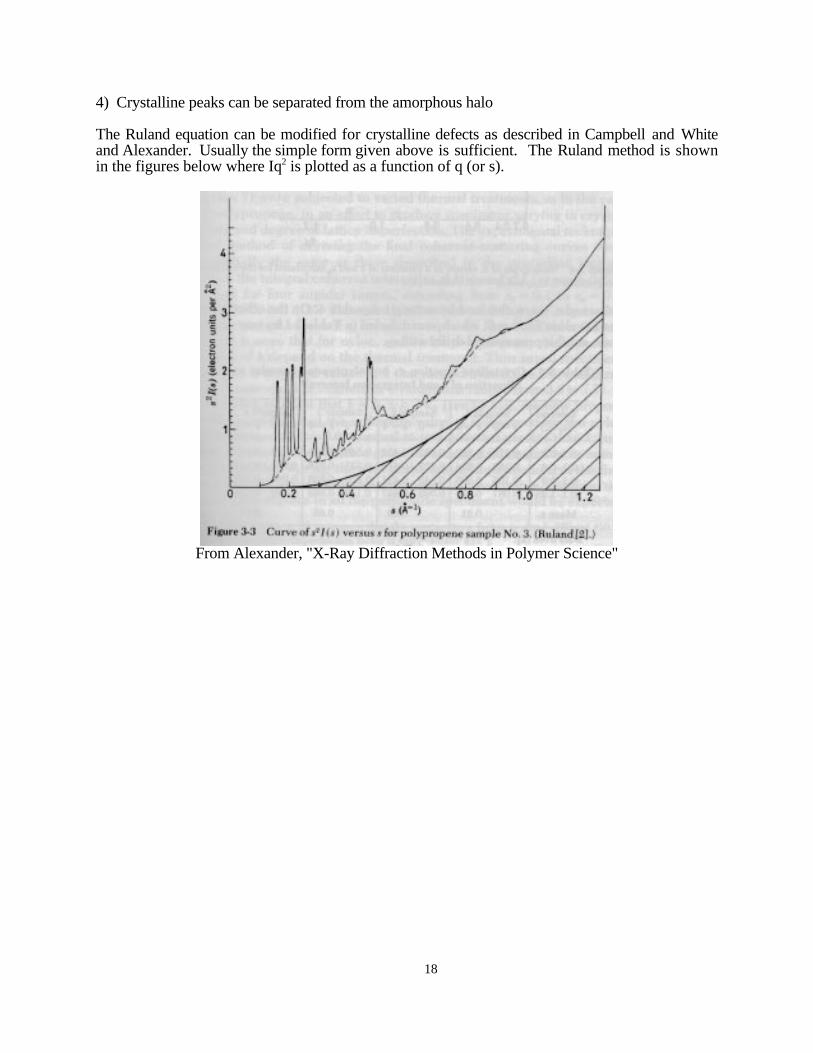
4) Crystalline peaks can be separated from the amorphous halo

The Ruland equation can be modified for crystalline defects as described in Campbell and Whiteand Alexander. Usually the simple form given above is sufficient. The Ruland method is shownin the figures below where Iq2 is plotted as a function of q (or s).

From Alexander, "X-Ray Diffraction Methods in Polymer Science"

19

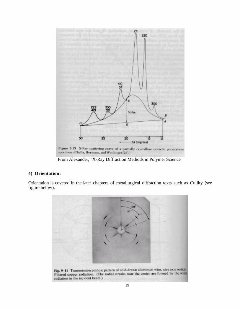
From Alexander, "X-Ray Diffraction Methods in Polymer Science"

4) Orientation:

Orientation is covered in the later chapters of metallurgical diffraction texts such as Cullity (seefigure below).

20

From Cullity, "Elements of X-Ray Diffraction

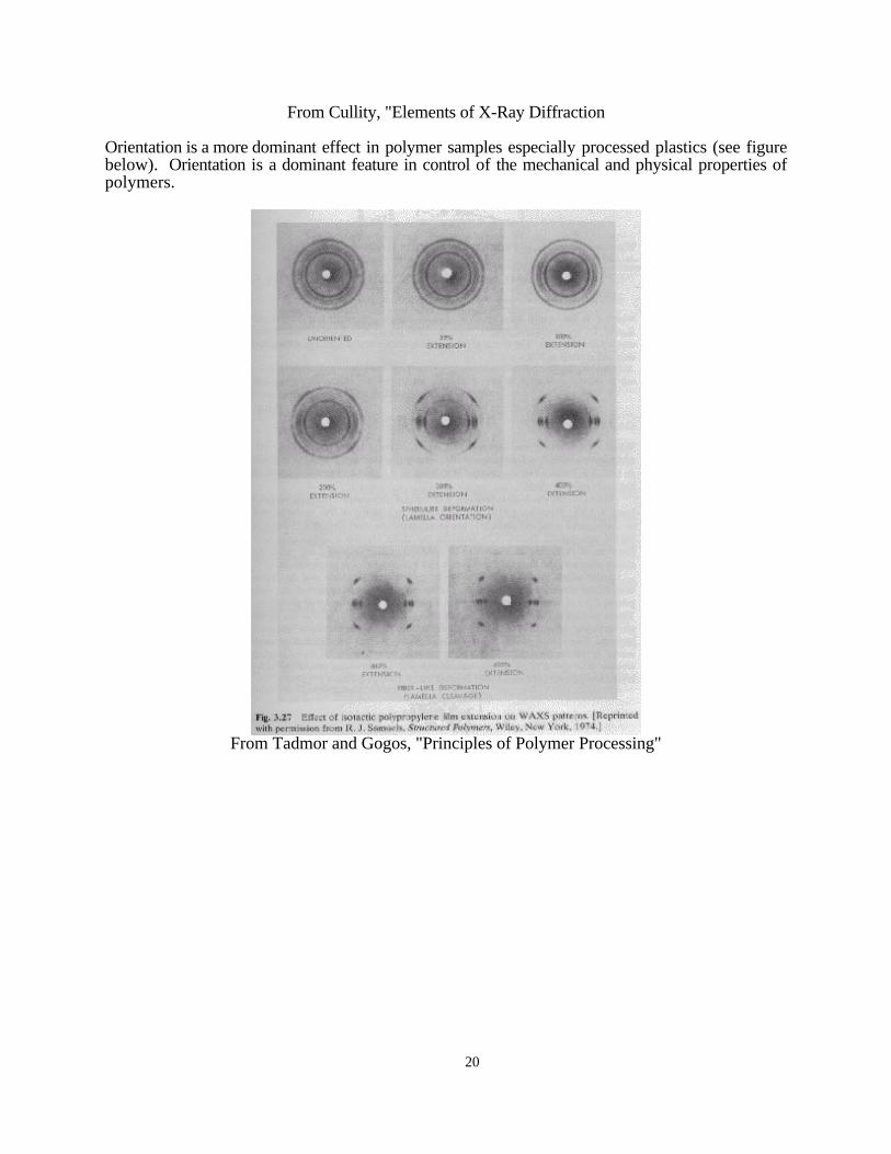
Orientation is a more dominant effect in polymer samples especially processed plastics (see figurebelow). Orientation is a dominant feature in control of the mechanical and physical properties ofpolymers.

From Tadmor and Gogos, "Principles of Polymer Processing"

21

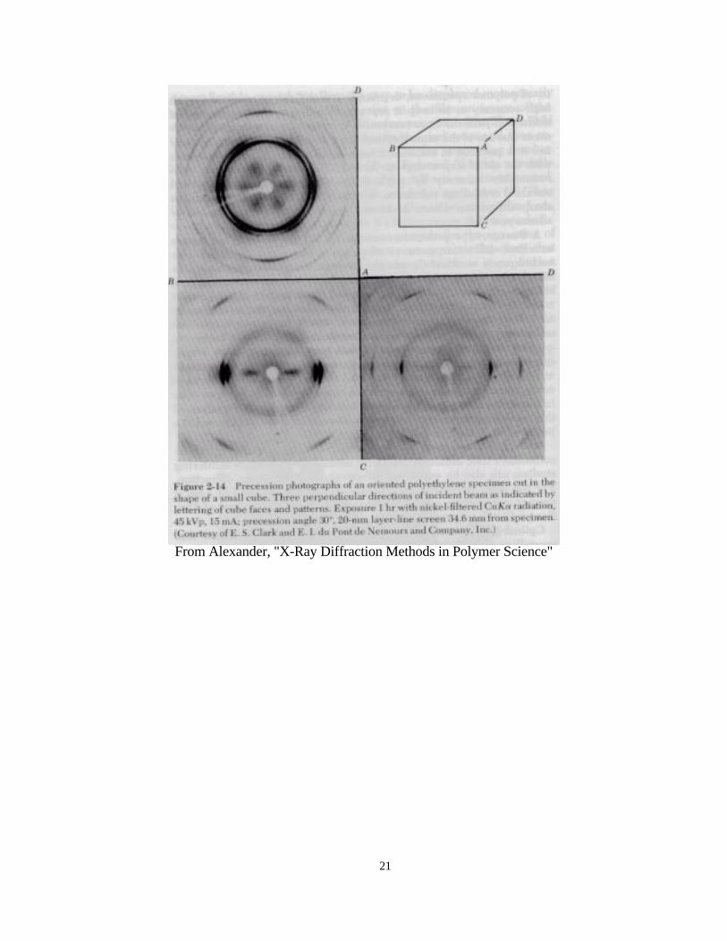
From Alexander, "X-Ray Diffraction Methods in Polymer Science"

22

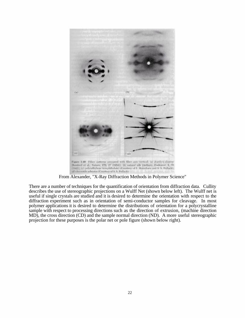
From Alexander, "X-Ray Diffraction Methods in Polymer Science"

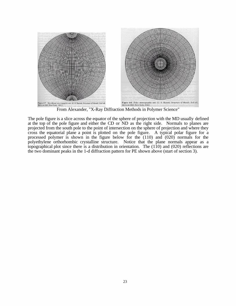
There are a number of techniques for the quantification of orientation from diffraction data. Cullitydescribes the use of stereographic projections on a Wulff Net (shown below left). The Wulff net isuseful if single crystals are studied and it is desired to determine the orientation with respect to thediffraction experiment such as in orientation of semi-conductor samples for cleavage. In mostpolymer applications it is desired to determine the distributions of orientation for a polycrystallinesample with respect to processing directions such as the direction of extrusion, (machine directionMD), the cross direction (CD) and the sample normal direction (ND). A more useful stereographicprojection for these purposes is the polar net or pole figure (shown below right).

23

From Alexander, "X-Ray Diffraction Methods in Polymer Science"

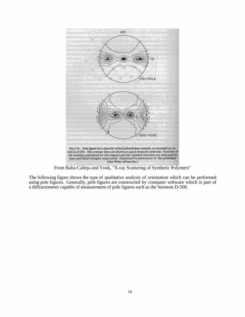
The pole figure is a slice across the equator of the sphere of projection with the MD usually definedat the top of the pole figure and either the CD or ND as the right side. Normals to planes areprojected from the south pole to the point of intersection on the sphere of projection and where theycross the equatorial plane a point is plotted on the pole figure. A typical polar figure for aprocessed polymer is shown in the figure below for the (110) and (020) normals for thepolyethylene orthorhombic crystalline structure. Notice that the plane normals appear as atopographical plot since there is a distribution in orientation. The (110) and (020) reflections arethe two dominant peaks in the 1-d diffraction pattern for PE shown above (start of section 3).

24

From Balta-Calleja and Vonk, "X-ray Scattering of Synthetic Polymers"

The following figure shows the type of qualitative analysis of orientation which can be performedusing pole figures. Generally, pole figures are constructed by computer software which is part ofa diffractometer capable of measurement of pole figures such as the Siemens D-500.

25

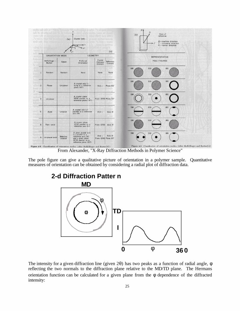
From Alexander, "X-Ray Diffraction Methods in Polymer Science"

The pole figure can give a qualitative picture of orientation in a polymer sample. Quantitativemeasures of orientation can be obtained by considering a radial plot of diffraction data.

2-d Diffraction Patter n

φ

I

MD

TD

0 36 0

φ

The intensity for a given diffraction line (given 2θ) has two peaks as a function of radial angle, φreflecting the two normals to the diffraction plane relative to the MD/TD plane. The Hermansorientation function can be calculated for a given plane from the φ dependence of the diffractedintensity:

26

f( ) cos11021

23 1= −( )φ

where <cos2φ> is the average cosine squared weighted by the intensity as a function of the radialangle for the (110) plane. The Hermans orientation function has the behavior that f = 1corresponds to perfect orientation in the φ = 0 direction, f = 0 for random orientation and f = -1/2

for perfect orientation normal to the φ = 0 direction. If the orientation function is calculate fororthogonal axis such as the a, b, and c unit cell directions for the PE unit cell then fa + fb + fc = 0.The orientation function for the unit cell vectors can be determined from geometry if the angularrelationship between a plane normal and the unit cell direction is known. <cos2φ> is calculated by:

cos

, sin cos

, sin

( )

( )

( )

2110

1102

0

2

110

0

2φ

φ θ φ φ φ

φ θ φ φ

π

π=( )

( )

∫

∫

I d

I d

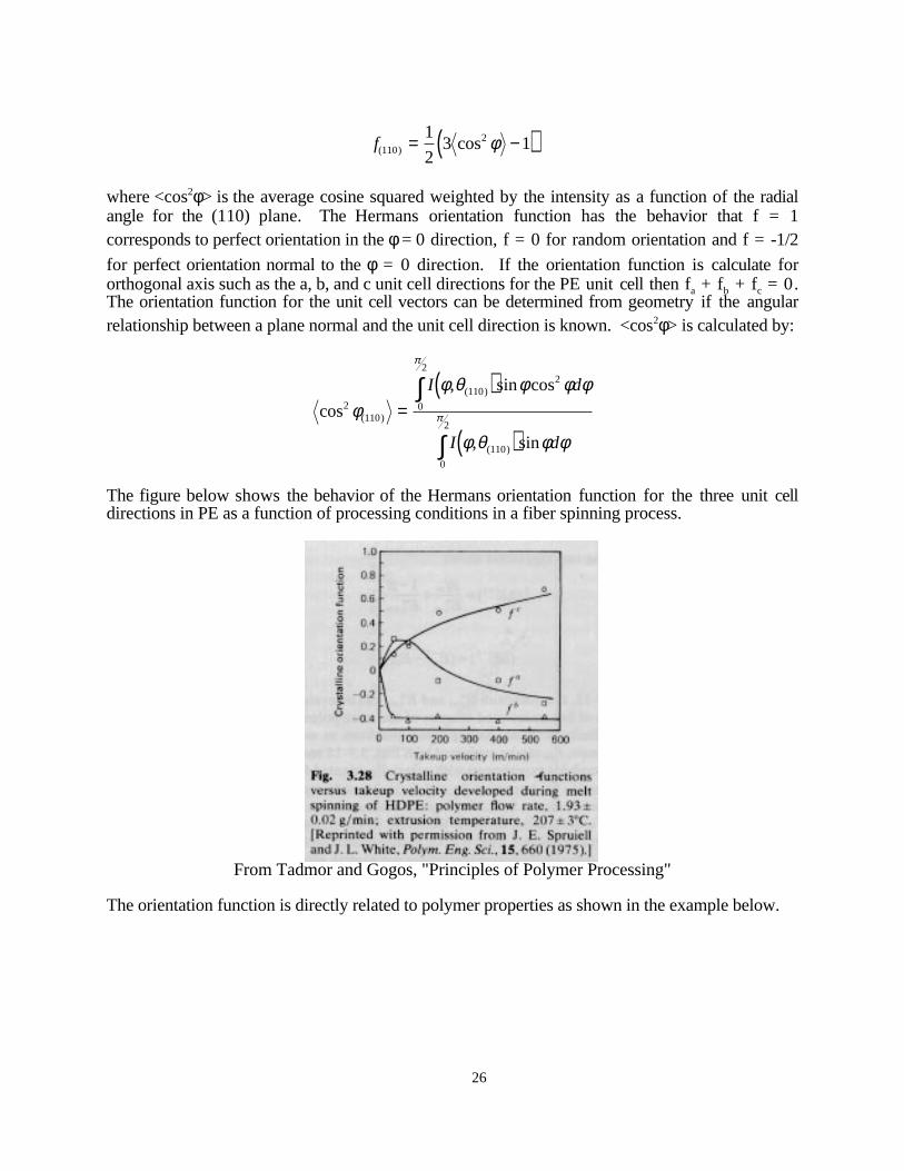
The figure below shows the behavior of the Hermans orientation function for the three unit celldirections in PE as a function of processing conditions in a fiber spinning process.

From Tadmor and Gogos, "Principles of Polymer Processing"

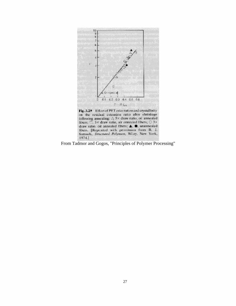
The orientation function is directly related to polymer properties as shown in the example below.

27

From Tadmor and Gogos, "Principles of Polymer Processing"