Methods Guide FINAL - worldagroforestry.org · Decision analysis methods guide Agricultural policy for nutrition Cory Whitney, ... including medical ... Diversity of household diets

Decision analysis methods guideAgricultural policy for nutrition

Cory Whitney, Keith Shepherd, Eike Luedeling

Decision analysis methods guide

Agricultural policy for nutrition

Cory Whitney, Keith Shepherd, Eike Luedeling

ii

LIMITED CIRCULATION

Correct citation: Whitney C, Shepherd K, Luedeling E. 2018. Decision analysis methods guide; Agricultural policy for nutrition. Working Paper No. 275. World Agroforestry Centre, Nairobi. http://dx.doi.org/10.5716/WP18001.PDF Titles in the Working Paper Series aim to disseminate interim results on agroforestry research and practices and stimulate feedback from the scientific community. Other publication series from the World Agroforestry Centre include the Trees for Change series, Technical Manuals and Occasional Papers. Published by the World Agroforestry Centre United Nations Avenue PO Box 30677, GPO 00100 Nairobi, Kenya Tel: +254(0)20 7224000, via USA +1 650 833 6645 Fax: +254(0)20 7224001, via USA +1 650 833 6646 Email: [email protected] Internet: www.worldagroforestry.org © World Agroforestry Centre 2018 Working Paper No. 275 The views expressed in this publication are those of the authors and not necessarily those of the World Agroforestry Centre. Articles appearing in this publication may be quoted or reproduced without charge, provided the source is acknowledged. All images remain the sole property of their source and may not be used for any purpose without written permission of the source.

Some parts of this working paper are shared as supplementary materials in the publication: Whitney CW, Lanzanova D, Muchiri C, Shepherd KD, Rosenstock TS, et al. 2018. Probabilistic decision tools for determining impacts of agricultural development policy on household nutrition. Earth’s Future

iii

About the authors

Cory Whitney, Centre for Development Studies (ZEF), University of Bonn, Genscherallee 3, 53113 Bonn, Germany/World Agroforestry Centre (ICRAF), PO Box 30677, Nairobi 00100, Kenya

Keith Shepherd, World Agroforestry Centre (ICRAF), PO Box 30677, Nairobi 00100, Kenya

Eike Luedeling, University of Bonn, Institut für Nutzpflanzenwissenschaften und Ressourcenschutz (INRES), Auf dem Hügel 6, 53121 Bonn, Germany/World Agroforestry Centre (ICRAF), PO Box 30677, Nairobi 00100, Kenya

iv

Abstract It is often very difficult to make accurate projections about how interventions will affect the real world and to use such projections to develop effective implementation plans, monitor progress and evaluate project impacts. This is due to a variety of factors including lack of data, complex impact pathways and risks and uncertainties that are difficult to factor into intervention planning. Scientific approaches to produce reliable impact projections are rarely applied in agricultural development, but Decision Analysis techniques commonly used in other fields have the potential to improve development decisions. This working paper outlines a Decision Analysis approach that can help decision makers efficiently allocate resources to enhance the effectiveness of policy decisions.

The procedures outlined in this publication feature the construction of causal models – models that describe the mechanisms through which intervention impacts will be delivered – that are co-developed by experts, stakeholders and analysts through facilitated participatory processes. These models are then formalized as Bayesian Network (BN) models, a modelling approach that has been widely applied in a range of disciplines, including medical sciences, genetics, environmental sciences and legal reasoning. BNs allow for the formal representation of causal models, such as intervention impact pathways. They can work effectively with incomplete information, combine expert knowledge with other sources of information and allow for adequate consideration of risk.

This paper illustrates the use of participatory workshops that convene experts on the systems, stakeholders involved in ongoing or prospective projects and analysts. These teams can jointly develop impact pathways for the interventions, which can be formalized into quantitative BN models. After several rounds of feedback elicitation and the inclusion of data from experts and other sources, stochastic simulations can be run to determine the likely impacts of the interventions. Results can be presented back to stakeholders for feedback.

Through the tools presented in this working paper, critical uncertainties in the models of intervention impact pathways can be identified. These high-value variables can determine uncertainty about project outcomes. Further measurement or disaggregation of these variables can support decision-making processes.

By demonstrating improved intervention decisions with little additional investment and improved tools for intervention decision modelling, we hope that this approach will be widely adopted and used to enhance the efficacy of development activities.

Keywords Decision Analysis, Bayesian Networks, Probabilistic Modelling, Nutrition, Hunger, Micronutrient Deficiency

v

Acknowledgements This work was funded by Competitive Research Grants to Develop Innovative Methods and Metrics for Agriculture and Nutrition Actions (IMMANA), grant number 1.36. IMMANA is funded by the UK government. We also acknowledge the support of the CGIAR Research Program on ‘Water, Land and Ecosystems’.

vi

Table of Contents

About the authors ................................................................................................................................. iiiAbstract ................................................................................................................................................ ivAcknowledgements ................................................................................................................................vList of figures ....................................................................................................................................... viList of tables ........................................................................................................................................ viiList of acronyms and abbreviations ................................................................................................... viiiIntroduction ............................................................................................................................................1

Predicting impacts of agriculture for nutrition activities ...................................................................1Decision Analysis ..................................................................................................................................3

Bayesian Networks ............................................................................................................................4Steps in the Decision Analysis process ..................................................................................................6

Decision framing ...............................................................................................................................6Generating a graphical model ............................................................................................................6Calibration training ............................................................................................................................8Model quantification .........................................................................................................................9

Example of a Bayesian Network ..........................................................................................................11Value of Information analysis .........................................................................................................13

The decisionSupport package ..............................................................................................................16Monte Carlo analysis .......................................................................................................................22

The AgenaRisk software ......................................................................................................................23Creating a Bayesian Network in AgenaRisk ...................................................................................23Value of Information calculation in AgenaRisk ..............................................................................24

Conclusion ...........................................................................................................................................26References ............................................................................................................................................27

List of figures Figure 1. Summary of the decision modelling process ........................................................................... 3Figure 2. The process used for eliciting graphical representations of decisions from expert groups to

be used in developing a Bayesian Network .................................................................................... 8Figure 3. Example of a tool for translating expert knowledge into a Conditional Probability Table

(CPT) for use in a Bayesian Network ........................................................................................... 10Figure 4. Example of a Bayesian Network for household nutrition impacts of a policy strategy (Vision

2040) in Uganda. ........................................................................................................................... 12Figure 5. Example of a filled input sheet for translating expert knowledge on Food Preferences ....... 17Figure 6. Interface of AgenaRisk software with example model of probabilities for different states of

Diversity of household diets under the Ugandan Government’s decision to implement Vision 2040 .............................................................................................................................................. 23

Figure 7. Example of a utility node as a partitioned expression filled with arithmetic values in the AgenaRisk software ...................................................................................................................... 24

Figure 8. Example of the input sheet for the VoI Analysis in the AgenaRisk software ....................... 25

vii

List of tables Table 1. Calculation of the expected value of perfect information for a Bayesian Network model of

utility values for value of diverse diets ......................................................................................... 14Table 2. Conditional probability table from the decisionSupport R code ............................................ 18Table 3. Legend for columns of the conditional probability table from the decisionSupport R code .. 19Table 4. Conditional probability table for Food Preferences under Uganda’s Vision 2040 development

decision. Strength of response ...................................................................................................... 20Table 5. Probabilities for different states of Food Preferences under the scenario that the Ugandan

Government’s Vision 2040 is implemented ................................................................................. 22

viii

List of acronyms and abbreviations AIE Applied Information Economics BN Bayesian Network CI Confidence Interval CPTs Conditional Probability Tables EKE Expert Knowledge Elicitation EMV Expected Monetary Value EVPI Expected Value or Perfect Information ICRAF World Agroforestry Centre IMMANA Innovative Methods and Metrics for Agriculture and Nutrition Actions INRES Institut für Nutzpflanzenwissenschaften und Ressourcenschutz MND Micronutrient Deficiency NPT Node Probability Table UK United Kingdom VoI Value of Information ZEF Centre for Development Studies

1

Introduction The development community faces increasing demand to credibly link research and development activities with progress towards the envisioned outcomes (Shepherd, Luedeling and Whitney, under review). Improved planning tools for interventions that target complex systems are urgently needed, especially in developing countries where data are scarce and uncertainties about decision outcomes are large. However, especially where quantitative impact predictions are requested, stakeholders are often left guessing about development outcomes, because they lack reliable tools to forecast impacts. Methodologies that address these uncertainties could transform the way development is done and greatly enhance the efficacy of its activities. Such methods could stimulate thorough scrutiny of research priorities and direct resources to where they lead to the greatest impacts (Luedeling and Shepherd, 2016). However, for this positive effect to materialize, the development community needs better approaches for planning for impact.

One of the central difficulties in planning for impact is dealing with uncertainty. It is rarely possible to accurately predict the impacts of agriculture for nutrition actions and other types of interventions. Many of the important factors that determine these impacts, such as adoption rates, yield increases, the performance of a particular tree or crop in a new environment and future weather, are highly uncertain. Additionally, many development interventions are implemented in risky environments, where extreme weather events, conflict, poor anticipation of cultural preferences, political interference or other risk factors can dramatically disrupt progress at any time (Luedeling et al., 2015).

Making impact projections in this environment, especially where precise numbers are expected, is very difficult and researchers and development workers often find themselves in an ethical quagmire, torn between the perceived need to honestly evaluate risks and the temptation to let wishful thinking guide their estimates. The latter may lead to overly optimistic assumptions and high impact projections that could raise the chance of political and donor support but are essentially unrealistic. This conflict of interest is not only a problem for project proponents – it also compromises the ability of stakeholders to compare impact ‘promises’ across proposals or reported impacts by different projects.

For research that is actually worth doing, results cannot be forecast with certainty (otherwise the research would not be necessary). However, what is currently lacking is a set of reliable methods to produce robust impact projections that take into account the host of uncertainties and risks that research and development activities are faced with. Such methods should be based on quantitative representations of impact pathways that capture the causal mechanisms of impact delivery. This publication aims to provide documentation for disseminating an approach based on Bayesian Networks (BNs) for impact pathway modelling. It seeks to establish Bayesian Networks (BNs) as a widely used analysis tool for development decisions related to agriculture for nutrition.

Predicting impacts of agriculture for nutrition activities Many activities in agricultural research and development aim at improving nutrition, but they are often unable to clearly articulate how nutrition objectives will be achieved and to what degree. Agricultural systems in developing countries are complex and few agricultural interventions can be expected to have an impact on such systems in a linear way. Thus, there is a need for new approaches to analyse the impacts of agricultural interventions on food and nutrition systems.

The success of an intervention will always depend on a number of factors that interact in ways that would be difficult or impossible to predict with precision. Some examples of these difficult-to-measure factors are the so-called ‘intangible’ factors, such as people’s perceptions of healthy food and their food preferences. The nutritional status of a country’s population is determined by many such

2

factors, including, not only, the nutritional value of the food people eat, but also a complex interplay between the food environment, household economics, health, education and agricultural value chains (Waage, Hawkes and Turner, 2012). Thus, many pathways may have the potential to improve national nutrition, for example, through higher nutrient contents in crops (DellaPenna, 1999; Nestel, Bouis, Meenakshi and Pfeiffer, 2006), greater nutritional diversity (Hoddinott and Yohannes, 2002) or improved awareness about childhood nutrition (Ruel, Alderman and Maternal, 2013). For any given context, however, it is difficult to decide a priori, which pathway will be most effective. Some pathways may not produce positive outcomes at all, if, for instance, the value chain degrades the nutritional value of the food, or if certain foods never reach vulnerable groups (e.g. children or lactating women).

Credible impact pathways regarding agriculture for nutrition should reflect their complexity. However, there is currently a severe shortage of practical methods that support credible analysis of these complex systems. Most conventional scientific approaches are unable to deal with this complexity. Opportunities for controlled trials are very limited, especially at low cost and simple statistical tools (regressions, correlations) do not provide much information about the way that drivers of agricultural systems are related to nutritional (and other) outcomes.

Use and analysis of impact pathways have helped to illustrate how interventions function, where they are lacking and what can be done to improve them. Leroy, Ruel and Verhofstadt (2009), for example, used impact pathway models to review the effect of cash transfer programs on child nutrition outcomes. Olney, Talukder, Iannotti, Ruel and Quinn (2009), used impact pathway models to evaluate the maternal and child health and nutrition effects of a homestead food production program in Cambodia and found that household-level benefits from the program did not translate into significant improvements in maternal and child health and nutrition. Both studies found a major gap in implementer and stakeholder knowledge about how the programs improve nutrition and identified this as a major obstacle to the interventions.

This paper provides a step-by-step guide to help synthesize expert knowledge and other sources of information into BN models that provide credible probabilistic projections of the impact of decisions. The methods described can be applied to multiple nutrition outcomes. The resulting models, as well as the participatory process from which they emerge, can be used to define useful metrics for monitoring progress towards nutrition outcomes. To achieve this, the working paper demonstrates a Bayesian approach, which seeks to express the current state of uncertainty on the main factors that affect to a decision, to help focus the measurement effort on areas that could narrow uncertainty, thus reducing ambiguity in the decision. Analysts can then update BNs based on the new information.

Whether a factor is seemingly easy or difficult to measure or has existing data available has no bearing on its inclusion. Omitting an important factor is essentially prescribing it as valueless. This is then complemented with innovative group work techniques aimed at eliciting expert knowledge to construct a logical framework to describe system interactions and outcomes (i.e., an impact pathway). Expert knowledge is thereby used to generate BN model structures (Bolger and Rowe, 2015; Kuhnert, Martin and Griffiths, 2010; Papakosta, Xanthopoulos and Straub, 2017) which are then integrated into model calculations (cf. Yet et al., 2016).

3

Decision Analysis Decision Analysis provides a framework for development research. Its objective is to facilitate better decisions by gaining insights into what actions could most increase multiple benefits given stakeholder preferences, while minimizing costs and risks. Abbas and Howard (2015) illustrate how the foundations of Decision Analysis provide the norms for decision-making. The basic Decision Analysis approach seeks to increase benefits and decrease risks on a continuous basis through the intervention planning and implementation process. The insights gained through the Decision Analysis approach include better understanding of the magnitude of the trade-offs among different development objectives relative to the preferences of different stakeholder groups. The ultimate aim is to ensure clarity of action for decision makers

The basic steps in the Decision Analysis process (Figure 1) address the questions of both why and how decisions are formulated and factors are measured. Hubbard (2014) outlines some of these approaches as part of his Applied Information Economics (AIE), dubbed the ‘Universal Modelling Approach’, since AIE has the basic premise that if something has an effect, this effect must be observable and if it is observable, it must be measurable. Decision Analysis and AIE are a collection of decision theory and risk analysis tools which use:

• Calibrated probability assessment (discussed in more detail in the section Calibration training)

• Value of additional information calculations applied to uncertain variables in a decision model, the results of which will reveal where to focus efforts to reduce uncertainty (e.g. by model refinement or by making further measurements)

• Empirical methods applied according to the information value of the measurement. Figure 1 presents a technical diagram of the Decision Analysis process adapted from Shepherd et al. (under review). The process outlined is followed in cooperation with key stakeholders and experts to improve the design of policy and interventions and monitor their impacts. The loop in the top half of the diagram describes the process that evaluates different alternatives in relation to the decision goals, whereas the lower loop uses value of information analysis to determine what should be measured to clarify the decision. There are iterative feedback loops throughout the process.

Figure 1. Summary of the decision modelling process, illustrating the sequence of activities in the decision modelling approach (Adapted from Shepherd et al., under review)

The merits of the application of the Decision Analysis tools for development decisions have been further described by Luedeling and Shepherd (2016), who point out that Decision Analysis solves the

4

problem of data gaps, which has often prevented research from comprehensively and holistically forecasting decision impacts. The approach allows explicit consideration of risks and variability.

Decision Analysis tools allow for decision-making that draws on all appropriate sources of evidence rather than rule out intangible and hard-to-measure aspects of a decision. Luedeling and Shepherd (2016) note that, in Decision Analysis, a model should include all the factors and all the important decision impacts that experts consider relevant, regardless of data availability. Shepherd et al. (2015) point out that Decision Analysis tools are particularly useful in development contexts, where data are often sparse. One very useful aspect of the approach is that expert knowledge can be used to fill in the knowledge gaps and avoid missing important factors when making decisions on development interventions.

Bayesian Networks Bayesian Networks (BNs) are a powerful tool for analysing causal relationships in complex systems, for integrating different sources of knowledge and for dealing effectively with imperfect information. BNs constructed with participation from key stakeholder groups could provide a rapid and robust means of applying existing knowledge to forecast intervention outcomes. This technique is practically absent from the planning of agricultural interventions for nutrition outcomes, even though it is well suited for many of the analytic challenges that researchers in this field have been struggling with. Introduction of BNs into this field could greatly enhance the way projects are planned, monitored and evaluated.

BNs have been in use since the 18th century to determine the probability of an event based on prior knowledge about the event. According to Nielsen and Jensen (2009), BNs are directed acyclic graphs consisting of nodes, arcs and probability tables underlying the nodal relationships. This means that BNs are based on direct causal relationships and do not contain logical loops. Instead, they are formulated as directed and acyclic models, as in a family tree. A BN is a network of probabilistic relationships between variables (known as nodes in the Bayesian nomenclature), referred to as child and parent nodes based on their arrangement in the model (cf. Figure 4). Conditional Probability Tables (CPTs) are the core elements of BN models (Fenton and Neil, 2012). They are used to define the probabilities for each state of each child node conditional on its parents (Papakosta et al., 2017). This allows analysts and experts to represent qualitative nodes as abstractions of the underlying continuous quantities. As an example, when developing a BN about nutrition in Uganda, the variable Food Preferences represents a family’s preference for diverse and nutritious food, which was considered important by experts, but proved difficult to quantify. Therefore, it is represented in the model as having five states, which describe the range of dietary preference, from poor nutrition to high nutrition: ‘very low’ (simple starchy staple-based diets, e.g. boiled tubers, rarely with small side-dishes, e.g. beans and some greens), ‘low’ (starchy staple diets with occasional small side-dishes), ‘medium’ (starchy staples commonly eaten with side-dishes, as well as fruits and vegetables), ‘high’ (balanced diets rich in fruits, vegetables and animal-based foods) and ‘very high’ (diets that are extremely rich in nutrients and micronutrients). The CPT for this variable is populated with the probabilities for these different states given the states of the parents Location and Nutrition awareness (shown in Figure 4).

BN models are distinct from other forms of statistical models, in that they focus on determining an optimal graphical model to describe probabilistic inter-relationships among processes rather than on specific measurement data. These models are a multivariate technique, which can accommodate one or many dependent variables. The approach can be used to investigate risk factors and causal pathways, which is important in health-related systems (cf. Lewis and McCormick, 2012). The key distinction between standard multivariate analyses and BN models is that multivariate regressions seek to identify covariates associated with some outcome variables. BN models, on the other hand, attempt to not only identify associated variables, but also separate them into those that have a direct and those that have an indirect influence on the outcome variables (Lewis, 2012). This gives BN

5

models the potential to reveal far more about key features of complex systems (Constantinou, Yet, Fenton, Neil and Marsh, 2016; Lewis and McCormick, 2012) and may make them preferable to standard approaches for inferring statistical dependencies from complex observational data (Korb and Nicholson, 2004; Lewis and McCormick, 2012). According to studies such as Papakosta et al. (2017), another major advantage of BN models is that they facilitate integration of information from various sources into a single model. Yet et al. (2016) also demonstrate how BNs can be used to build predictive models of impact pathways that incorporate both hard data and expert judgment. Despite their widespread applications, BNs have not been exploited in the agriculture/nutrition domain. Yet, they are highly suited to this context. For example, Henderson and Burn (2004) illustrate how BNs are able to combine information from various sources, such as hard data and expert knowledge, into comprehensive causal models that result in more accurate impact forecasts than using data or expert knowledge alone.

This working paper discusses how to adapt and apply BN-based procedures for developing comprehensive impact pathways for agriculture for nutrition interventions. It demonstrates the ability of such BNs to aid in decision-making under multiple uncertainties and imperfect information. The paper acts as a guide to construct robust and reliable impact models by convening experts in the fields of agriculture and nutrition, as well as related disciplines. The modelling approach has several advantages. First, it allows for comparison of the prospects of different interventions for improving nutrition security, thus helping to identify the most promising approaches. Second, it allows for the consideration of risks to intervention success and identification of weak links in the impact pathway that require particular attention by intervention planners. Third, it permits the inclusion of difficult-to-measure factors that are commonly omitted from models, thus opening up opportunities for holistic research. Lastly, it helps prioritize metrics that would be critical to monitor during implementation – especially those variables that have large residual uncertainty and a large potential impact on intervention outcomes.

6

Steps in the Decision Analysis process

Decision framing Decision framing is the first part of the decision analysis process. It determines the boundaries of a decision and is the most important aspect of making a good decision. Decision framing starts by identifying both a decision to be modelled and the relevant experts. This is not as simple as it sounds and should be undertaken carefully and with a lot of forethought. Consideration of the criteria that define a decision can help to add structure to this important step in the process: • It is a choice between two or more alternatives that involves an irrevocable allocation of

resources• It involves uncertainty (as we pointed out earlier, the analysis would not be necessary, if results

could be forecast with certainty)• It involves a decision maker or decision-making body (who will allocate resources or act).As Shepherd et al. (under review) point out, in order to achieve clarity in decision-making each of the above elements and the preferences of the decision maker, need to be carefully defined.

Once the decision has been identified, the decision analysts identify and convene relevant decision makers, stakeholders and any additional experts. A group of around 20 experts is a manageable size for a workshop. More than that can be cumbersome, especially when dealing with model building in plenary.

It is important to have a number of different types of knowledge holders involved in the development of the impact model. Therefore, expert selection should seek to gather experts with knowledge on as many aspects of the decision as possible. As Fenton and Neil (2012) indicate, expert knowledge is often vital in identifying critical, underlying causal factors that affect risks and opportunities that would otherwise be missed based on available data or statistical models. The experts selected for modelling agriculture for nutrition decisions should represent a mix of knowledge holders such as academic institutions (e.g. nutritionists and agronomists), government institutions, local villages and development organizations (see Luedeling and Whitney, 2017).

Generating a graphical model The next step in the Decision Analysis process is to jointly develop a decision model (Figure 1). In the workshop setting, it is important for the analyst to gather all the variables that the expert group agrees are logically important to describe the impact pathway of the decision and include them in the model. This should be done regardless of ease of measurement of the individual variables.

Before engaging in this process, the overall context for the model (the decision that was identified) should be explicitly defined and agreed upon during plenary discussions with the identified experts. Once this is done, building the graphical model can begin. In our approach, we start from the decision framing step through to the model development by asking experts to work together and peer-review each other’s work.

Bolger and Rowe (2015) and Bolger and Wright (2017) list the various challenges in handling expert knowledge, which include both poor judgment regarding probability and high levels of variation among experts. These problems occur because experts are not trained to formulate reliable representations of uncertainty, many lack experience with probability and few learn to express their uncertainty as probability distributions. Here, we outline several important steps that should be taken to aid in the process of collaboratively building model structures and making variable estimates. These will help to ensure accuracy in the process.

7

Collaborative approaches Tools are available to help overcome these problems. According to Bolger and Rowe (2015), it is possible to improve conditions for gathering expert knowledge. These include creating experiences for experts to make estimates for well-defined targets, giving them tools on which to base their estimates and offering regular and usable feedback about the accuracy of their estimates. According to Bolger and Wright (2017), experts can be a source of quality data about the future. Ensuring the quality of this data starts by selecting the best experts, training experts in the normative aspects of anticipation and combining judgments from several experts.

Here we illustrate some useful approaches for combining expert-estimated probability distributions, using the accumulated information from multiple experts. In this approach, a workshop is held and graphical models are developed by individual experts and then peer-reviewed by other experts. These approaches allow analysts to obtain as much information as possible and gather data that represent a summary of expert opinion. Clemen and Winkler (1999) and Bolger and Wright (2017) offer more examples of these tools in practice.

Figure 2 has been adapted from Whitney et al. (2018). It illustrates a process that can be used to elicit graphical representations of decisions from expert groups, to be used in developing a BN. This approach is generally outlined in the work of Iqbal and MacLean (2010), who consulted experts in repeated group meetings to build a BN for defoliation prediction by sawfly infestations in Newfoundland. Each expert was asked to create a BN model which was then peer-reviewed by other experts in the group. In our approach, the process begins with breaking the decision down into several important questions in plenary discussions. Random interchanging working groups of experts are then led through three stages of collaborative thinking for each question that is brought up. These are:

1. Consider the question alone. Experts are given a short time (usually a minute or two) for quiet reflection and writing of the question.

2. Share with an immediate neighbour. Experts are given some time (usually a few minutes) to compare notes and ideas on the question with another participant in the working group.

3. Share with working group and design. Working groups are given as much time as necessary to discuss and design a model of their collective understanding of the functional pathways related to the question.

The steps defined above and illustrated in Figure 2 are designed to help experts interact, brainstorm and reach a common understanding about impact pathways. Through this approach, they can explore details of the expected impacts, disaggregate the impact pathway into intermediate steps and identify all the influencing factors that they consider important to the decision (i.e., draw a model of nodes and edges; cf. Figure 4).

8

Figure 2. The process used for eliciting graphical representations of decisions from expert groups to be used in developing a Bayesian Network (Source: Whitney et al., 2018)

The iterative process of building a model in the workshop is illustrated in Figure 2. The steps are repeated until all experts have worked on each question and are satisfied that all specific relationships have been identified. Participants should be encouraged to discuss any factors they deem important for the decision, in particular, the various costs, benefits and risks associated with interventions, as well as the objectives and concerns of decision makers and stakeholders. The model should have the broad aim to describe the effects of agricultural decisions on specific nutrition outputs such as hunger (a.k.a. global energy and macronutrient deficiency).

Following this approach, it is important that the analysts have an overview of the process, with the objective of building a final working BN model in mind. Analysts should work to guide the experts so that they think about how model parameters interact in a logical way. For example, the work of Whitney et al. (2018) illustrates the use of the Expert Knowledge Elicitation (EKE) approach to build an impact model, which aims to deliver the probabilities for different states of malnutrition under a policy decision and to relate this directly to a monetary value for calculating variables of importance (see the section Value of Information analysis)

Resulting models can then be brought before the whole group of experts for plenary discussion and re-drawn, aiming for a common understanding about the relationships in each model. The end result should be one model per question with the contributions of all experts. These can then be combined into one large impact pathway model. Corrections and further feedback can be gathered for model verification as a final stage of model development.

Calibration training The next step of the modelling procedure is known as ‘calibration training’. Experts are trained, using well-established ‘calibration’ procedures, to estimate their state of uncertainty and thereby increase their capacity to provide accurate estimates by reducing errors of judgment. Through the process, experts learn to improve their ability to estimate their own state of uncertainty and thereby reduce errors of judgment, e.g. under-confidence or over-confidence (i.e. give correct estimates 90% of the time when they have 90% confidence, Hubbard, 2014). As both Hubbard (2014) and O’Hagan et al. (2006) demonstrate, through this training experts learn to minimize potential biases in probability estimation.

9

Calibration training consists of several exercises aimed at revealing the participants’ personal biases (over-confidence or under-confidence) by assessing their performance on a set of trivia questions. Through these exercises, experts are trained to assess their subjective uncertainty and express it as a Confidence Interval (CI). This interval has a predefined chance (e.g. 90%) of containing the right value. Perfectly calibrated people should get around 90% of the answers correct and any deviation (outside a narrow band of stochastic variation) from this optimal figure indicates estimation bias. Experts are calibrated through repetition and feedback on the exercises. The training is divided into several stages:

1. The concepts of calibration are presented to the participants, along with the empirical evidencethat assessing uncertainty is not a skill that arises automatically from experience but a generalskill that can be gained through training in quantification techniques.

2. Participants benchmark their “natural” skills in quantifying their own uncertainty. To this end,they take a short quiz aimed to help them determine their initial level of over-confidence.

3. Methods of self-calibration proposed by Hubbard (2014), are provided such as:

– The “equivalent bet test”: Participants are invited to imagine a spinning dial on a circlethat is 10% red and 90% green. They are asked to imagine that if the real answer fallswithin the range they selected, they win 100 dollars, or they can choose to spin the dialand if the arrow lands on green, they win 100 dollars. If they prefer the dial over thewheel they do not have 90% confidence in their answer (over-confident), whereas ifthey choose their answer instead of the wheel, their confidence level is higher than 90%(under-confident).

– The test of “considering two pros and two cons”: Participants are invited to imagine thatthe limits that they provided for their estimate range are wrong. They then considerdifferent possible explanations for why these are wrong and, if any insights arise, theyadjust accordingly.

– The “absurdity test”: Participants are invited to create distributions that they are sure arewildly broader than the actual 90% confidence range. They then slowly reduce theirranges down to a more reasonable distribution while considering the logic behind thereduction.

4. Participants work on two types of exercises: (1) 90% CI questions and (2) binary questions. Inthe 90% CI questions, they are asked to provide a range (a lower bound and an upper bound) forwhich there is a 90% chance that it includes the right answer. In the binary questions, theyanswer whether each of a series of statements is true or false and then give the probability theythink their answer is the right one. This is an iterative process: they give their answers, comparewith the true values and test again.

The examples given by Hubbard (2014) and Luedeling et al. (2015) show that through the use of these procedures, experts learn to give estimates that are neither too vague (under-confidence) nor too specific (over-confidence). The procedures seek to help participants become accurate estimators. Accuracy, in this context, does not mean precision, but rather refers to the ability to produce an accurate range of probable estimates of different possible states of the variables of interest. Therefore, the procedures outlined in this approach seek to provide experts with the skills necessary to represent uncertainty explicitly as probabilities of different possible states of the world.

Estimations of the node states within the BN can begin once the experts have been through the training and the analysts are satisfied that the experts are adequately calibrated. More examples of these calibration procedures and instructions on their application are provided in detail by Hubbard (2014).

Model quantification For final model quantification, the analyst converts the conceptual model into a mathematical model, translating stakeholder inputs into equations as accurately as possible. Following Luedeling et al. (2015), all estimates can then be consolidated into one single distribution for each model parameter.

10

As mentioned in the section, Bayesian Networks, BNs are based on simplified node structures, known as Conditional Probability Tables (CPTs), which specify the relationships between parent and child nodes. CPTs can sometimes contain large numbers of conditional probabilities, especially where several parents with multiple possible states are involved. Estimating large numbers of probabilities can be overwhelming for experts. For this reason, Fenton, Neil and Caballero (2007) warn that the overwhelming nature of this CPT filling process can lead to inconsistencies. The works of Cain (2001) and Marcot, Steventon, Sutherland and McCann (2006) also warn that these inconsistencies run the risk of leading to unreliable models. Luckily, several tools are available to simplify the process of filling CPTs. For example, Fenton et al. (2007) found that experts find it easier to understand and express relationships through the use of weighted averages and ranked nodes. Rather than fill CPTs directly, experts can be asked to provide a typical distribution of each variable (prior probability) together with the strength of the response and a weighting factor for each state of the child node and each state of the parent nodes. Figure 3 highlights an example of an input sheet that can be used to elicit expert knowledge from four main aspects of the variable of interest:

• Prior distributions for the node of interest (prior probability)• Relative influence of each the parents (in the example in Figure 3 there are two parents but there

can be any number)• Effects of each state of the parent nodes• Strength of the response (cf. Figure 3).

Figure 3 presents an example of a tool for translating expert knowledge into a Conditional Probability table (CPT) for use in a Bayesian Network (see Whitney et al., 2018).

Figure 3. Example of a tool for translating expert knowledge into a Conditional Probability Table (CPT) for use in a Bayesian Network (Source Whitney et al., 2018)

This approach helps analysts to gather expert knowledge for all model parameters. These parameters can then be used to calculate the CPTs (see Luedeling and Whitney, 2017) using the likelihood method as described by Hansson and Sjökvist (2013). As outlined by Kemp-Benedict, Bharwani, Rosa, Krittasudthacheewa and Matin (2009) experts can provide influence weights rather than whole tables of probabilities.

Once completed and verified with the literature and other sources, the BN can be shared with experts again to verify its logical consistency and receive final feedback.

Software resources for direct application of these calculations are presented later in the publication. Procedures for producing CPTs from these inputs have been implemented in the decisionSupport package for R (2017).

11

This is outlined in the section The decisionSupport package.

Software for modelling Bayesian Networks can be used to build interactive graphical models and for calculating the BN. In the section, The AgenaRisk software, we outline some of the tools available in AgenaRisk (Fenton and Neil, 2016), useful for calculating the BN model.

Example of a Bayesian Network A possible BN model for a policy strategy in Uganda is illustrated in Figure 4. The model includes 29 nodes to describe the impact pathway from the strategy decision (Vision 2040; Figure 4 left) to household nutrition (hunger and micronutrient deficiency; Figure 4 right). The model includes two policy-related nodes (nutritional awareness and promotion of exports), five economic nodes (land tenure, location [proxy for access to goods and services], exported production, occupation and food access), seven social variables (displacement of farmers, nutritional education and sensitization, traditional knowledge, nutrition awareness, diversity of agricultural systems, food preferences and nutritional quality) and seven nodes related to both micronutrients (production, availability, demand, consumption and deficiency [MND]) and macronutrients (production, availability, demand, consumption and hunger) (Luedeling and Whitney, 2017).

12

Figure 4. Example of a Bayesian Network for household nutrition impacts of a policy strategy (Vision 2040) in Uganda. Probabilities are shown for outcome variables and variables with the highest value of information (boxes with bars). Green bars show the probabilities for node states under the decision not to implement Vision 2040 and blue bars show probabilities for node states under the scenario that it is implemented1

1 The full model is available on the Harvard DataVerse (Luedeling and Whitney, 2017)

13

The causal relationships identified in Figure 4 were elicited from expert groups (following the process shown in Figure 2). The graphical representation was then programmed into a BN model. Following the steps outlined in the section Model quantification, the CPTs were then filled with calibrated expert estimates for each node and edge. This was written into a programmable BN model developed in AgenaRisk (Fenton and Neil, 2016), one of many commercial software options for BN model development. The model was published on the Harvard DataVerse along with a detailed explanation of the data (probabilities and formulas) behind the model (see Luedeling and Whitney, 2017).

Value of Information analysis

As discussed in the section, Generating a graphical model, it is important for the analyst to gather all the variables that the expert group agrees are logically important to describe the impact pathway of the decision and include them in the model. This should happen for several reasons, the most important of which is that the final development outcomes are generally strongly dependent on variables with high uncertainty. These uncertain variables often include important ‘intangible’ factors such as behavioural, institutional and policy factors and are likely to be brought up by the experts as part of their discussions of impact pathways. Part of the value of the Decision Analysis approach is that it directs attention and performance monitoring to such factors, identified by their high information value. When a model has been programmed in the appropriate software and no clearly preferable decision emerges from the model results, Value of Information (VoI) analysis can be used to reveal what further information is needed to narrow uncertainty and clarify a decision. It is expressed as the amount that a rational decision maker would be willing to pay for that knowledge before making a decision. VoI is a central concept of Decision Analysis. It is used to guide decisions on the level of complexity to be considered in a decision model and the need for further measurement to clarify decision alternatives. VoI can be estimated by analysing the uncertainties in all the variables that have a bearing on a decision. According to Abbas and Howard (2015), VoI can also be described as the value of clairvoyance.

VoI analysis can be used to determine whether additional information on certain input variables in the BN model could increase confidence about the emerging decision recommendation. The examples of Hubbard (2014) show that often, when value of information analysis is used to prioritize measurements, only a few variables may be relevant for the decision recommendation. Any further data collection should focus on those variables that can help to narrow the decision choices. Other examples, such as those of Constantinou et al. (2016) and Whitney et al. (2017), illustrate how the results of VoI analysis can be used to prioritize knowledge gaps that should most urgently be narrowed in order to improve certainty about a decision. Constantinou et al. (2016) also demonstrate that VoI can help decision makers ascertain if a decision outcome is dependent on – or independent of – any risk factors, thereby helping to focus any necessary follow-up research resources. More follow-up measurements and disaggregation of any identified variables can help inform the design and prioritization of future research and provide guidance about the best pathways for implementing the current decision.

Expected Value of Perfect Information The Expected Value of Perfect Information (EVPI) is one useful VoI tool. It is the difference between the expected value of a decision made with perfect information and the expected value of the decision with current imperfect information (Hubbard, 2014). The many examples presented by Hubbard (2014) and those of Felli and Hazen (2003) show how EVPI can help decision makers consider both the probability of change due to a decision and the resulting difference in payoff. Constantinou et al. (2016) demonstrate how EVPI can be calculated for BN models to identify a selected subset of important model variables. To achieve this, utility nodes are used to assign monetary value to model outputs (example shown in Table 1).

14

The Expected Monetary Value (EMV) is a key part of the EVPI calculation. It is the weighted average of the payoffs for a decision alternative, where weights are the probabilities of the different states of nature (Table 1). EVPI is the maximum amount that one should be willing to pay for additional information about the decision. EVPI = EVwithPI - max(EMV), meaning that EVPI is the expected value for the decision (payoff), if perfect information is available about the states of nature, minus the expected value for the decision if perfect information is not available.

A simple hypothetical example of a Value of Information (VoI) calculation, based on the Ugandan nutrition example, is presented in Table 1. This model is shown in Figure 4 and available on the Harvard DataVerse (Luedeling and Whitney, 2017). The table is populated with estimated values for different states of the Diversity of household diets based on the implementation of Vision 2040.

Table 1 shows the calculation of EVPI in a BN. The main part of the table is populated with a ‘utility value’ for diverse diets under each of the ‘states of nature’, e.g. the upper right value of -4 represents the utility value of low household dietary diversity in the scenario where decision makers decide not to implement Vision 2040. The likelihood of each of the states of Diversity of household diets is shown in the row labelled with Probability.

In Table 1, EMV is calculated for each state of the Vision 2040 decision by adding the utility values after multiplying them by the probability for each state of Diversity of household diets. The maximum EMV is the highest of these two (27.7). Expected value with perfect information (EV with PI) is calculated for each column by selecting the highest value for each state of Diversity of household diets (29.7). EVPI is calculated using the resulting values EVPI = EVwithPI - max(EMV). Table 1. Calculation of the expected value of perfect information (EVPI) for a Bayesian Network model of utility values for value of diverse diets

Diversity of household diets Expected Monetary Value (EMV)

States Low Medium High

Vision 2040 implemented -4 42 60 EMV = 0.35(-4)+0.55(42)+0.1(60)=27.7

Vision 2040 not implemented -11 31 80 EMV = 0.35(-11)+0.55(31)+0.1(80)=21.2

Probability 0.35 0.55 0.1 Max EMV = 27.7

EV with PI 0.35(-4)+0.55(42)+0.1(80)=29.7

EVPI 29.7-27.7=2 Source Whitney et al., 2018.

Variables that have large uncertainty and a large potential impact on outcomes will have high information values. Information values also point decision makers to places where they could adjust the intervention design to reduce risks and improve outcomes, in addition to providing guidance to analysts on where to increase model complexity. With the new information, the model can be run again. The process is repeated, until decision makers feel confident that they can make a well-informed decision (Figure 1).

Value of information analysis provides an efficient, iterative approach to information collection, as measurements are only made as far as needed and lowest-cost options are tried first. As a first step, experts and analysts can work on decomposing model variables into sub-variables that are easier to estimate in an attempt to narrow uncertainty. If there is still residual information value, then the analysts may try further literature review or consulting with more experts to further narrow the uncertainty.

In this approach, analysts only need to design physical measurements or surveys if the other steps are insufficient. Even in the event that more data needs to be gathered, small sample sizes may be sufficient to reduce uncertainty and reveal a clear decision. Value of information analysis also tells decision makers how much they should consider spending on these measurements. From applying probabilistic decision modelling on over 80 diverse problems, Hubbard (2014) observed that only a few variables typically had

15

high information value in any given decision and interestingly, they were rarely variables receiving current measurement effort.

16

The decisionSupport package The decisionSupport package (Luedeling and Goehring, 2017) in the R programming language (R core team, 2017) performs several useful functions for the development of BNs. One particularly useful tool is the likelihood method for estimating CPTs. The likelihood method works by defining the likelihood that states of several qualitative variables lead to states of another qualitative one.

Figure 3 gives an example of a tool for gathering input from experts and translating their knowledge into a Conditional Probability Table (CPT) for use in a Bayesian Network (adapted from Whitney et al., 2018).

For application in developing CPTs, there are three useful functions within the decisionSupport package:

• The make_CPT function creates Conditional Probability Tables for Bayesian Network nodes from parameters that (for complex nodes) can be more easily elicited from experts than the full table. The function uses the Likelihood method, as described by Hansson and Sjökvist (2013). Tables are created from the relative weights of all parents, rankings for all parents, a parameter (b) for the sensitivity of the child node and a prior distribution (for the child node).

• The sample_CPT function randomly chooses a state of a categorical variable, based on a Conditional Probability Table (CPT; a component of Bayesian Network models) that expresses the probability of each possible state in relation to the states of other categorical variables. Given information on the state of all parent variables, the function uses the appropriate probability distribution to draw a random sample for the state of the variable of interest.

• The sample_simple_CPT function creates Conditional Probability Tables for Bayesian Network nodes from parameters that (for complex nodes) can be more easily elicited from experts than the full table. The function uses the Likelihood method. The function combines the make_CPT and sample_CPT functions, but only offers limited flexibility.

All the above functions are described in detail in the documentation of the decisionSupport package. Here we will demonstrate the application of the make_CPT function using data gathered with an input sheet shown in Figure 3. As described in the section Model quantification, this sheet helps analysts and experts to represent qualitative nodes as abstractions of the underlying continuous quantities. Figure 5 presents an input sheet that has been filled by experts for building a CPT in the BN shown in Figure 4. In this model, the variable Food Preferences was considered important by experts, but was difficult to quantify. Therefore, it is represented as having the states ‘very low’, ‘low’, ‘medium’, ‘high’ and ‘very high’. Through the use of the input sheet and the make_CPT function, the CPT for this variable can be populated with the probabilities for these different states given the influence and states of the parents Location and Nutrition awareness.

17

Figure 5. Example of a filled input sheet for translating expert knowledge on Food Preferences given the states of the parents Location and Nutrition awareness into a Conditional Probability Table (CPT) for use in a Bayesian Network.

The values gathered from experts are shown in Figure 5. These can be translated into a CPT through the use of the make_CPT function in R using the R code shown below. Entering this code into R yields two outputs. The first ($CPT) contains conditional probabilities with the states of Food Preferences as rows. The second output from the make_CPT function is a descriptor for the columns in the CPT called $column_legend. These columns are based on the different combined states of the parents Location and Nutrition awareness.

18

R code with resulting CPT and legend tables library(decisionSupport) make_CPT(parent_effects=list(c(-1,-0.5,0, 0.5, 1), c(1,0.6,-1,-1,-1,-0.6)), parent_names=c("Nutrition awareness","Location"), parent_weights=c(1,1),b=2,child_prior=c(0.2,0.3,0.3, 0.1, 0.1), child_states=c("Very low","Low","Medium", "High", "Very high"), parent_states=list(c("Very low","Low","Medium", "High", "Very high"), c("Same rural area","Different rural area", "Forest, wetland etc.","Small urban area", "Large urban area","Other countries")))

The output from the R code above is shown in Table 2 (CPT values) and Table 3 (legend for column names). Table 2. Conditional probability table from the decisionSupport R code

col_1 col_2 col_3 col_4 col_5 col_6 col_7 col_8 col_9 col_10 col_11 col_12 col_13 col_14 col_15

Very low 0.2 0.25 0.45 0.45 0.45 0.4 0.15 0.19 0.39 0.39 0.39 0.33 0.1 0.14 0.32

Low 0.3 0.32 0.34 0.34 0.34 0.34 0.26 0.29 0.34 0.34 0.34 0.34 0.22 0.26 0.34

Medium 0.3 0.28 0.17 0.17 0.17 0.2 0.31 0.3 0.2 0.2 0.2 0.23 0.31 0.32 0.24

High 0.1 0.08 0.03 0.03 0.03 0.04 0.12 0.1 0.04 0.04 0.04 0.05 0.15 0.13 0.06

Very high 0.1 0.07 0.01 0.01 0.01 0.02 0.15 0.11 0.02 0.02 0.02 0.04 0.21 0.16 0.04

col_16 col_17 col_18 col_19 col_20 col_21 col_22 col_23 col_24 col_25 col_26 col_27 col_28 col_29 col_30

Very low 0.32 0.32 0.27 0.07 0.1 0.26 0.26 0.26 0.21 0.05 0.06 0.2 0.2 0.2 0.16

Low 0.34 0.34 0.33 0.18 0.21 0.33 0.33 0.33 0.31 0.14 0.17 0.3 0.3 0.3 0.27

Medium 0.24 0.24 0.27 0.3 0.31 0.27 0.27 0.27 0.3 0.27 0.3 0.3 0.3 0.3 0.31

High 0.06 0.06 0.07 0.17 0.15 0.08 0.08 0.08 0.1 0.18 0.17 0.1 0.1 0.1 0.12

Very high 0.04 0.04 0.06 0.28 0.22 0.06 0.06 0.06 0.09 0.36 0.3 0.1 0.1 0.1 0.14

19

Table 3. Legend for columns of the conditional probability table from the decisionSupport R code

col_1 col_2 col_3 col_4 col_5 col_6

Nutrition awareness Very low Very low Very low Very low Very low Very low

Location Same rural area Different rural area Forest, wetland etc. Small urban area Large urban area Other countries


Nutrition awareness Low Low Low Low Low Low



Nutrition awareness Medium Medium Medium Medium Medium Medium



Nutrition awareness High High High High High High



Nutrition awareness Very high Very high Very high Very high Very high Very high


To help with the interpretation of the R output, the full CPT for Food Preferences in Table 4 has been included, together with the input data for prior probabilities for all nodes, strength of response (b) and relative influence of the parent nodes (see Luedeling and Whitney, 2017).

20

Table 4. Conditional probability table for Food Preferences under Uganda’s Vision 2040 development decision. Strength of response (b) = 2

Nutrition Awareness Location Food preferences

(Relative influence =1) (Relative influence =1) (diversity and sufficiency)

Very low Low Medium High Very high

Prior * 0.20 0.30 0.30 0.10 0.10

States Impact distribution States Impact

distribution

Very Low -1

Same rural area 1.00

0.2 0.3 0.3 0.1 0.1

Different rural area 0.60

0.25 0.32 0.28 0.08 0.07

Forest, Wetland, parks etc. -1.00

0.45 0.34 0.17 0.03 0.01

Small urban area -1.00

0.45 0.34 0.17 0.03 0.01

Large urban area -1.00

0.45 0.34 0.17 0.03 0.01

Other countries -0.60 0.25 0.32 0.28 0.08 0.07

Low -0.5


0.15 0.26 0.31 0.12 0.15


0.19 0.29 0.3 0.1 0.11


0.39 0.34 0.2 0.04 0.02


0.39 0.34 0.2 0.04 0.02


0.39 0.34 0.2 0.04 0.02

Other countries -0.60 0.19 0.29 0.3 0.1 0.11

Medium 0


0.1 0.22 0.31 0.15 0.21


0.14 0.26 0.32 0.13 0.16


0.32 0.34 0.24 0.06 0.04


0.32 0.34 0.24 0.06 0.04


0.32 0.34 0.24 0.06 0.04

Other countries -0.60 0.14 0.26 0.32 0.13 0.16

High 0.5


0.07 0.18 0.3 0.17 0.28


0.1 0.21 0.31 0.15 0.22


0.26 0.33 0.27 0.08 0.06


0.26 0.33 0.27 0.08 0.06


0.26 0.33 0.27 0.08 0.06

21

Nutrition Awareness Location Food preferences

(Relative influence =1) (Relative influence =1) (diversity and sufficiency)

Very low Low Medium High Very high

Prior * 0.20 0.30 0.30 0.10 0.10

States Impact distribution States Impact

distribution

Other countries -0.60 0.1 0.21 0.31 0.15 0.22

Very High 1


0.05 0.14 0.27 0.18 0.36


0.06 0.17 0.3 0.17 0.3


0.2 0.3 0.3 0.1 0.1


0.2 0.3 0.3 0.1 0.1


0.2 0.3 0.3 0.1 0.1

Other countries -0.60 0.06 0.17 0.3 0.17 0.3

22

The resulting probabilities for Food Preferences under the scenario that the Ugandan

Government’s Vision 2040 is implemented are shown in Table 5 and in Figure 4.

Table 5. Probabilities for different states of Food Preferences under the scenario that the Ugandan

Government’s Vision 2040 is implemented

State Probability Very Low 0.26 Low 0.30 Medium 0.26 High 0.09 Very high 0.09

Monte Carlo analysis The reader may also find it useful to explore the integration of CPTs within a Monte Carlo

analysis. Monte Carlo is another commonly used Decision Analysis tool that applies a

repeated random sampling algorithm on decision inputs to obtain a distribution of possible

decision outputs. There are many benefits of the Monte Carlo approach. For example, an

impact model similar to that shown in Figure 4 could be used to run a Monte Carlo with

outcome variables as a distribution of plausible values (e.g. Vitamin A per person per day)

rather than a probability of nutrient or micronutrient deficiency (as is currently shown in

Figure 4). We will not give an exhaustive explanation of the implementation of these tools

here but have described them in detail in a number of publications (see the References

section) and through the vignettes linked to the decisionSupport package (Luedeling and

Goehring, 2017).

23

The AgenaRisk software

There are several commercial software options for modelling Bayesian Networks. These

packages offer a visual interaction with the programmable BN model. We will not give an

exhaustive example of how to implement these here, as the software comes with an easy-to-

follow user manual. Instead, we will briefly describe the use of the AgenaRisk software for

programming and analysis of the expert-knowledge-based Decision Analysis we have

described above. Readers may refer to the AgenaRisk user manual and software package for

more information about the many useful applications and several example models (Fenton

and Neil, 2016).

Figure 6. Interface of AgenaRisk software with example model of probabilities for different states of Diversity of

household diets under the Ugandan Government’s decision to implement Vision 2040

Creating a Bayesian Network in AgenaRisk Figure 6 displays a screenshot of the main interface from the AgenaRisk package (Fenton and

Neil, 2016). The top row of icons is for the overall model; the second row of icons is for

individual nodes. The large white space to the right is where the graphical model can be

drawn and the column of icons to the left offers the tools used for drawing the graphical

model (in AgenaRisk, graphical models are called ‘Risk Maps’).

The lower three icons in the left vertical toolbar in Figure 6 can be used to create nodes and

edges. Nodes can be created based on CPTs (the top circle) or based on calculations (bottom circle, marked with ! ). The nodes can have a number of different states. The symbols on the

upper right corner of each of these nodes indicate the type of node that is used (B=boolean, R=ranked, ! =arithmetic). The arrow icon from the left icon bar can be selected to connect

24

nodes. The arrow represents causal relationships and connects parents to child nodes, thereby

changing the underlying probability tables.

Each node within the graphical model includes an underlying probability table, referred to as

a Node Probability Table (NPT) in AgenaRisk (what is commonly called CPT, in the

literature and in this text). The window for filling in the node values can be accessed by

selecting the node and clicking on the ! symbol in the second row of icons at the top of the

interface shown in Figure 6.

The CPT can be populated with probability values manually, or by copying and pasting the

CPT results from the make_CPT function. The first table of outputs from the decisionSupport

tool is shown in the section R code with resulting CPT and legend tables.

For arithmetic nodes the values can also be entered manually. Figure 7, for example, presents

the node probability table for the arithmetic node labelled ‘Utility’ in Figure 6. To enter the

values for this node we select the ‘Partitioned Expression’ option in ‘NPT editing Mode’.

The utility values are entered manually by double-clicking on each cell within the table shown

in Figure 6. The values shown are the same as those given in Table 1.

Figure 7. Example of a utility node as a partitioned expression filled with arithmetic values in the AgenaRisk

software

Value of Information calculation in AgenaRisk As is shown in Table 1, the causal relationship between the decision node and the uncertainty

node is expressed in the utility node. In order to identify the value of information, we can

calculate the EVPI of this decision, as per Table 1.

25

Figure 8. Example of the input sheet for the Value of Information Analysis in the AgenaRisk software

To do this, we select the function dubbed ‘Value of Information Analysis’ from the ‘Tools’

menu in AgenaRisk. When selecting this option with the BN shown in Figure 6 the ‘Value of

Information Analysis’ option leads to the input sheet shown in Figure 8. There are several

settings options for the function shown in Figure 8:

• ‘Select the Risk Object’: This applies to models with several risk objects. We only have one risk object so we do not use this option here.

• ‘Select the Scenario’: This applies to models with several observations that have been

entered (e.g. decision ‘yes’ or ‘no’). In this example the decision node ‘Vision 2040’ is set to equal (50/50 chance) probability so it does not matter which scenario we choose.

• ‘Select Decision, Uncertainty and Utility Nodes’: In this example we have shifted the

nodes from a list on the left to the appropriate boxes on the right, i.e., ‘Vision 2040’ is

the decision node, ‘Diversity of household diets’ is the uncertainty node and ‘Utility’ is

the utility node.

Selecting ‘Run’ on this window will create a document titled ‘VoIReport.html’ showing the

results and means of an EVPI calculation. This has the same results and a similar format to

Table 1.

26

Conclusion

In this paper, we have attempted to outline some tools for the adaptation and application of

Bayesian Networks to agriculture for nutrition development contexts. Decision Analysis is an

important paradigm for development research. The approach of using BN models promises to

be an effective strategy for dealing with complex systems, multiple impact pathways,

uncertain and incomplete information and other current constraints to meaningful quantitative

impact projections.

The many factors that determine the nutritional impact of agricultural interventions are

interconnected in various ways and there are often clear causal connections between them.

Most traditional research approaches, such as regression analysis, controlled trials, etc., fare

poorly in complex and multi-factorial situations and results from modelling exercises that

adopt deterministic perspectives on complex systems are often not credible, because they rely

on a host of simplifying assumptions. However, rational prioritization among ‘agriculture for

nutrition’ actions requires an evaluation approach that can accommodate the complex

relationships and thereby credibly translate agricultural activities into nutritional outcomes.

We see the potential for great benefits to arise from an approach such as BNs within the

Decision Analysis paradigm. These approaches can integrate existing data with expert opinion

and other sources of information. This can be a considerable improvement in development

research, especially for considering causal relationships in potential intervention impacts. We

hope that this publication will contribute to the wider application of these tools to agriculture

for nutrition decisions.

More information and resources are available through the referenced materials, in the

decisionSupport package for R (Luedeling and Goehring, 2017) and the AgenaRisk software

(Fenton and Neil, 2016), as well as on the Harvard DataVerse (Luedeling and Whitney,

2017).

27

References

Abbas, A. E., Howard, R. A. 2015. Foundations of decision analysis: 832. NY, NY: Prentice Hall.

Bolger, F., Rowe, G. 2015. The aggregation of expert judgment: Do good things come to those who

weight. Risk Analysis, 35(1): 5–11.

Bolger, F., Wright, G. 2017. Use of expert knowledge to anticipate the future: Issues, analysis and

directions. International Journal of Forecasting, 33(1): 230–243.

Cain, J. 2001. Planning improvements in natural resource management. guidelines for using Bayesian

Networks to support the planning and management of development programmes in the water

sector and beyond: 136. Crowmarsh Giford, Wallingford, Oxon, UK: Centre for Ecology;

Hydrology.

Clemen, R. T., Winkler, R. L. 1999. Combining probability distributions from experts in risk analysis.

Risk Analysis, 19(2): 187–203.

Constantinou, A., Yet, B., Fenton, N., Neil, M., Marsh, W. 2016. Value of information analysis for

interventional and counterfactual Bayesian Networks in forensic medical sciences. Artificial

Intelligence in Medicine, 66: 41–52.

DellaPenna, D. 1999. Nutritional genomics: Manipulating plant micronutrients to improve human

health. Science, 285(5426): 375–379.

Felli, J. C., Hazen, G. B. 2003. Sensitivity analysis and the Expected Value of Perfect Information.

Medical Decision Making, 23(1): 97.

Fenton, N., Neil, M. 2012. Risk assessment and Decision Analysis with Bayesian Networks: 503. Boca

Raton, Florida: CRC Press.

Fenton, N., Neil, M. 2016. AgenaRisk professional version 7.0. Revision 3451 VOI.

Fenton, N., Neil, M., Caballero, J. 2007. Using ranked nodes to model qualitative judgments in

Bayesian networks. IEEE Transactions on Knowledge and Data Engineering, TKDE-0095-

0206.R2: 1–11.

Hansson, F., Sjökvist, S. 2013. Modelling expert judgement into a Bayesian Belief Network. PhD

thesis, Lund University, Lund, Sweden.

Henderson, J., Burn, R. 2004. Uptake pathways: The potential of Bayesian Belief Networks to assist

the management, monitoring and evaluation of development-orientated research. Agricultural

Systems, 79(1): 3–15.

Hoddinott, J., Yohannes, Y. 2002. Dietary diversity as a food security indicator, vol. Discussion Paper

136: 1–2. Washington, DC: International Food Policy Research Institute (IFPRI).

Hubbard, D. W. 2014. How to measure anything: Finding the value of intangibles in business, vol.

Second Edition: 301. Hoboken, New Jersey: John Wiley and Sons.

Iqbal, J., MacLean, D. A. 2010. Prediction of balsam fir sawfly defoliation using a Bayesian network

model. Can. J. for. Res., 40(12): 2322–2332.

28

Kemp-Benedict, E., Bharwani, S., Rosa, E. de la, Krittasudthacheewa, C. and Matin, N. 2009.

Assessing water-related poverty using the sustainable livelihoods framework. Stockholm:

Stockholm Environment Institute.

Korb, K. B., Nicholson, A. E. 2004. Bayesian artificial intelligence.: 365. London: Chapman and

Hall/CRC Press UK.

Kuhnert, P., Martin, T., Griffiths, S. 2010. A guide to eliciting and using expert knowledge in Bayesian

ecological models. Ecology Letters, 13(7): 900–914.

Leroy, J. L., Ruel, M., Verhofstadt, E. 2009. The impact of conditional cash transfer programmes on

child nutrition: A review of evidence using a programme theory framework. Journal of

Development Effectiveness, 1(2): 103–129.

Lewis, F. I. 2012. Bayesian Networks as a tool for epidemiological systems analysis: 610–617. Zurich:

Zurich Open Repository; Archive, University of Zurich.

Lewis, F., McCormick, B. 2012. Revealing the complexity of health determinants in resource-poor

settings. American Journal of Epidemiology, 176(11): 1051–1059.

Luedeling, E., Whitney, C. W. 2017. Probabilistic causal models for nutrition outcomes of agricultural

actions - Uganda model. Harvard DataVerse, World Agroforestry Centre - ICRAF Dataverse,

ICRAF Decision Analysis DataVerse.

Luedeling, E., Goehring, L. 2017. decisionSupport – quantitative support of decision-making under

uncertainty. Contributed package to the R programming language. version 1.103.2.

Luedeling, E., Shepherd, K. 2016. Decision-focused agricultural research. Solutions, 7(5): 46–54.

Luedeling, E., Oord, A. L., Kiteme, B., Ogalleh, S., Malesu, M., et al. 2015. Fresh groundwater for

Wajir - ex-ante assessment of uncertain benefits for multiple stakeholders in a water supply

project in northern Kenya. Frontiers in Environmental Science, 3, article 16: 1–18.

Marcot, B. G., Steventon, J. D., Sutherland, G. D., McCann, R. K. 2006. Guidelines for developing and

updating Bayesian Belief Networks applied to ecological modelling and conservation.

Canadian Journal of Forest Research, 36(12): 3063–3074.

Nestel, P., Bouis, H. E., Meenakshi, J., Pfeiffer, W. 2006. Biofortification of staple food crops. The

Journal of Nutrition, 136(4): 1064–1067.

Nielsen, T. D., Jensen, F. V. 2009. Bayesian Networks and decision graphs: XVI, 448. New York:

Springer Science and Business Media.

Olney, D. K., Talukder, A., Iannotti, L. L., Ruel, M. T., Quinn, V. 2009. Assessing impact and impact

pathways of a homestead food production program on household and child nutrition in

Cambodia. Food and Nutrition Bulletin, 30(4): 355–369.

O’Hagan, A., Buck, C. E., Daneshkhah, A., Eiser, J. R., Garthwaite, P. H., et al. 2006. Uncertain

judgements: Eliciting experts’ probabilities. West Sussex: John Wiley and Sons.

Papakosta, P., Xanthopoulos, G., Straub, D. 2017. Probabilistic prediction of wildfire economic losses

to housing in Cyprus using Bayesian Network analysis. International Journal of Wildland

Fire, 26(1): 10–23.

29

Ruel, M., Alderman, H., Maternal, C. N. S. G. 2013. Nutrition-sensitive interventions and programmes:

How can they help to accelerate progress in improving maternal and child nutrition. Lancet,

382(9891): 536–551.

Shepherd, K., Hubbard, D., Fenton, N., Claxton, K., Luedeling, E., et al. 2015. Development goals

should enable decision-making. Nature, 523(7559): 152–154.

Shepherd, K., Luedeling, E., Whitney, C. W. under review. A Decision Analysis framework for

development planning and performance measurement: Application to land restoration

investments.

R Core Team. 2017. R: A language and environment for statistical computing [r version 3.4.1 (2017-

06-30) “Single Candle”], 3.4.1.

Waage, J., Hawkes, C., Turner, R. 2012. Current and planned research on agriculture for improved

nutrition: A mapping and a gap analysis. A report for DFID: 48. London: Leverhulme Centre

for Integrative Research on Agriculture; Health (LCIRAH).

Whitney, C. W., Lanzanova, D., Muchiri, C., Shepherd, K. D., Rosenstock, T. S., et al. 2018.

Probabilistic decision tools for determining impacts of agricultural development policy on

household nutrition. Earth’s Future

Whitney, C. W., Tabuti, J. R., Hensel, O., Yeh, C.-h., Gebauer, J., et al. 2017. Home gardens and the

future of food and nutrition security in southwest Uganda. Agricultural Systems, 154: 133–

144.

Yet, B., Constantinou, A., Fenton, N., Neil, M., Luedeling, E., et al. 2016. A Bayesian Network

framework for project cost, benefit and risk analysis with an agricultural development case

study. Expert Systems with Applications, 60: 141–155.

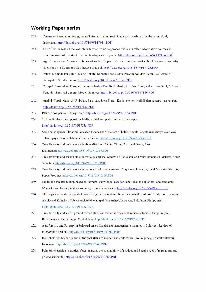
30

Working Paper series 257. Dinamika Perubahan Penggunaan/Tutupan Lahan Serta Cadangan Karbon di Kabupaten Buol,

Indonesia. http://dx.doi.org/10.5716/WP17011.PDF

258. The effectiveness of the volunteer farmer trainer approach vis-à-vis other information sources in

dissemination of livestock feed technologies in Uganda. http://dx.doi.org/10.5716/WP17104.PDF

259. Agroforestry and forestry in Sulawesi series: Impact of agricultural-extension booklets on community

livelihoods in South and Southeast Sulawesi. http://dx.doi.org/10.5716/WP17125.PDF

260. Petani Menjadi Penyuluh, Mungkinkah? Sebuah Pendekatan Penyuluhan dari Petani ke Petani di

Kabupaten Sumba Timur. http://dx.doi.org/10.5716/WP17145.PDF

261. Dampak Perubahan Tutupan Lahan terhadap Kondisi Hidrologi di Das Buol, Kabupaten Buol, Sulawesi

Tengah: Simulasi dengan Model Genriver http://dx.doi.org/10.5716/WP17146.PDF

262. Analisis Tapak Mata Air Umbulan, Pasuruan, Jawa Timur. Kajian elemen biofisik dan persepsi masyarakat.

http://dx.doi.org/10.5716/WP17147.PDF

263. Planned comparisons demystified. http://dx.doi.org/10.5716/WP17354.PDF

264. Soil health decision support for NERC digital soil platforms: A survey report


265. Seri Pembangunan Ekonomi Pedesaan Indonesia: Menanam di bukit gundul: Pengetahuan masyarakat lokal

dalam upaya restorasi lahan di Sumba Timur. http://dx.doi.org/10.5716/WP17356.PDF

266. Tree diversity and carbon stock in three districts of Kutai Timur, Pasir and Berau, East

Kalimantan http://dx.doi.org/10.5716/WP17357.PDF

267. Tree diversity and carbon stock in various land use systems of Banyuasin and Musi Banyuasin Districts, South

Sumatera http://dx.doi.org/10.5716/WP17358.PDF

268. Tree diversity and carbon stock in various land cover systems of Jayapura, Jayawijaya and Merauke Districts,

Papua Province http://dx.doi.org/10.5716/WP17359.PDF

269. Modelling tree production based on farmers’ knowledge: case for kapok (Ceiba pentandra) and candlenut

(Aleurites mollucana) under various agroforestry scenarios. http://dx.doi.org/10.5716/WP17361.PDF

270. The impact of land cover and climate change on present and future watershed condition. Study case: Tugasan,

Alanib and Kulasihan Sub-watershed of Manupali Watershed, Lantapan, Bukidnon, Philippines.


271. Tree diversity and above-ground carbon stock estimation in various land use systems in Banjarnegara,

Banyumas and Purbalingga, Central Java. http://dx.doi.org/10.5716/WP17363.PDF

272. Agroforestry and Forestry in Sulawesi series: Landscape management strategies in Sulawesi: Review of

intervention options. http://dx.doi.org/10.5716/WP17364.PDF

273. Household food-security and nutritional status of women and children in Buol Regency, Central Sulawesi,

Indonesia. http://dx.doi.org/10.5716/WP17365.PDF

274. Palm oil expansion in tropical forest margins or sustainability of production? Focal issues of regulations and

private standards. http://dx.doi.org/10.5716/WP17366.PDF

The World Agroforestry Centre is a centre of scientific excellence that harnesses the benefits of trees for people and the environment. Leveraging the world's largest repository of agroforestry science and information, it develops knowledge practices for farmers' fields through to the global sphere to ensure food security and environmental stabilty.

The Centre's vision is an equitable world where all people have viable livelihoods supported by healthy and productive landscapes. Its mission is to harness the multiple benefits trees provide for agriculture, livelihoods, resilience and the future of our planet, from farmers' fields through to continental scales.

United Nations Avenue, Gigiri • PO Box 30677 • Nairobi, 00100 • Kenya Telephone: +254 20 7224000 or via USA +1 650 833 6645

Fax: +254 20 7224001 or via USA +1 650 833 6646Email: [email protected] • www.worldagroforestry.org

Documents

Methods Guide FINAL - worldagroforestry.org · Decision analysis methods guide Agricultural policy for nutrition Cory Whitney, ... including medical ... Diversity of household diets