1

M. HauskrechtCS 2710 Foundations of AI

CS 2710 Foundations of AI

Lecture 7

Milos Hauskrecht

milos@pitt.edu

5329 Sennott Square

Methods for finding optimal

configurations

M. Hauskrecht

Search for the optimal configuration

Constrain satisfaction problem:

Objective: find a configuration that satisfies all constraints

Optimal configuration (state) problem:

Objective: find the best configuration (state)

The quality of a state: is defined by some quality measure that

reflects our preference towards each configuration (or state)

Our goal: optimize the configuration according to the quality

measure also referred to as objective function

2

M. HauskrechtCS 1571 Intro to AI

Search for the optimal configuration

Optimal configuration search problem:

• Configurations (states)

• Each state has a quality measure q(s) that reflects our

preference towards each state

• Goal: find the configuration with the best value

– Expressed in terms of the objective function

s*=argmaxs q(s)

If the space of configurations we search among is

• Discrete or finite

– then it is a combinatorial optimization problem

• Continuous

– then it solved as a parametric optimization problem

M. Hauskrecht

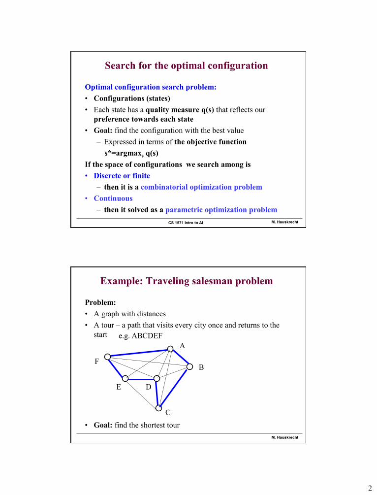
Example: Traveling salesman problem

Problem:

• A graph with distances

• A tour – a path that visits every city once and returns to the

start

• Goal: find the shortest tour

A

B

C

DE

F

e.g. ABCDEF

3

M. Hauskrecht

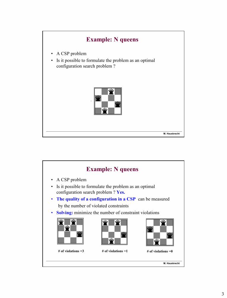
Example: N queens

• A CSP problem

• Is it possible to formulate the problem as an optimal

configuration search problem ?

M. Hauskrecht

Example: N queens

• A CSP problem

• Is it possible to formulate the problem as an optimal

configuration search problem ? Yes.

• The quality of a configuration in a CSP can be measured

by the number of violated constraints

• Solving: minimize the number of constraint violations

# of violations =0# of violations =3 # of violations =1

4

M. Hauskrecht

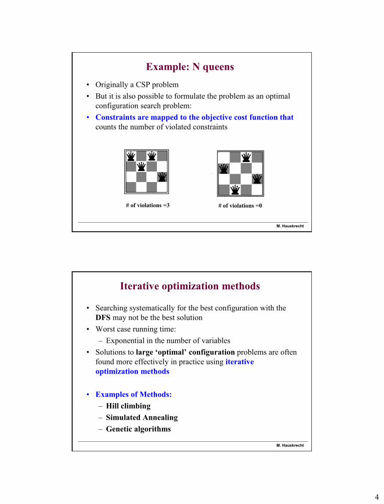
Example: N queens

• Originally a CSP problem

• But it is also possible to formulate the problem as an optimal

configuration search problem:

• Constraints are mapped to the objective cost function that

counts the number of violated constraints

# of violations =0# of violations =3

M. Hauskrecht

Iterative optimization methods

• Searching systematically for the best configuration with the

DFS may not be the best solution

• Worst case running time:

– Exponential in the number of variables

• Solutions to large ‘optimal’ configuration problems are often

found more effectively in practice using iterative

optimization methods

• Examples of Methods:

– Hill climbing

– Simulated Annealing

– Genetic algorithms

5

M. Hauskrecht

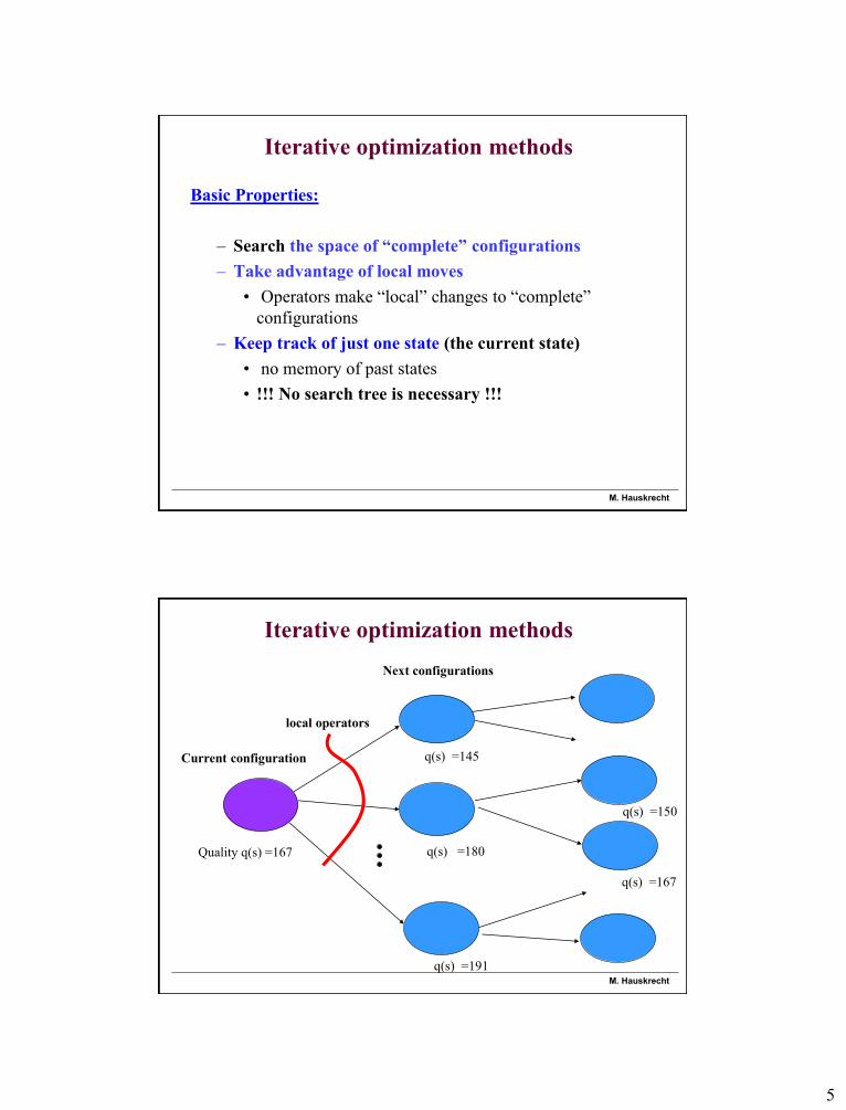
Iterative optimization methods

Basic Properties:

– Search the space of “complete” configurations

– Take advantage of local moves

• Operators make “local” changes to “complete”

configurations

– Keep track of just one state (the current state)

• no memory of past states

• !!! No search tree is necessary !!!

M. Hauskrecht

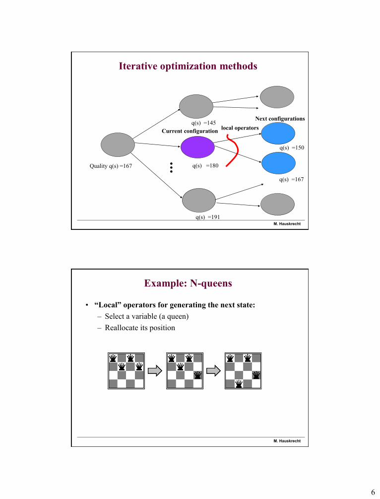
Iterative optimization methods

Current configuration

Quality q(s) =167

q(s) =145

q(s) =180

q(s) =191

Next configurations

local operators

q(s) =167

q(s) =150

6

M. Hauskrecht

Iterative optimization methods

Current configuration

Quality q(s) =167

q(s) =145

q(s) =180

q(s) =191

Next configurations

local operators

q(s) =167

q(s) =150

M. Hauskrecht

Example: N-queens

• “Local” operators for generating the next state:

– Select a variable (a queen)

– Reallocate its position

7

M. Hauskrecht

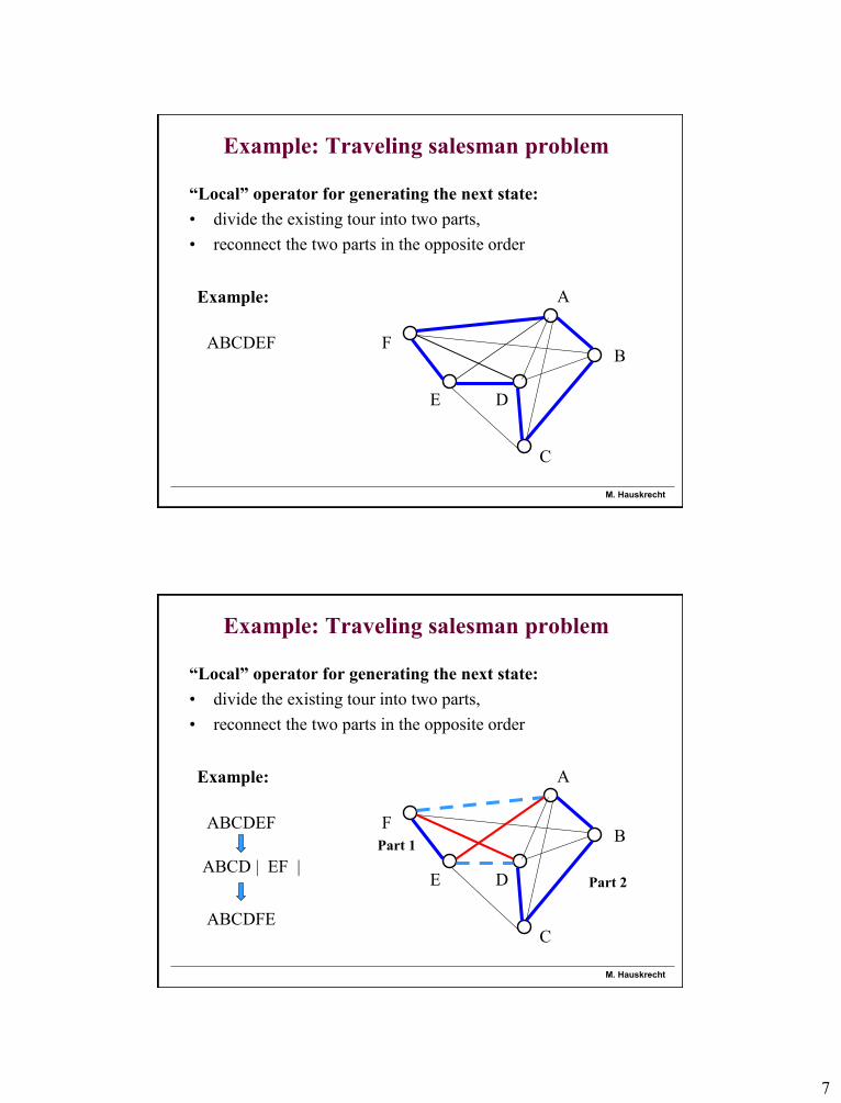
Example: Traveling salesman problem

“Local” operator for generating the next state:

• divide the existing tour into two parts,

• reconnect the two parts in the opposite order

A

B

C

DE

F

Example:

ABCDEF

M. Hauskrecht

Example: Traveling salesman problem

“Local” operator for generating the next state:

• divide the existing tour into two parts,

• reconnect the two parts in the opposite order

Part 1

Part 2

A

B

C

DE

F

Example:

ABCD | EF |

ABCDFE

ABCDEF

8

M. Hauskrecht

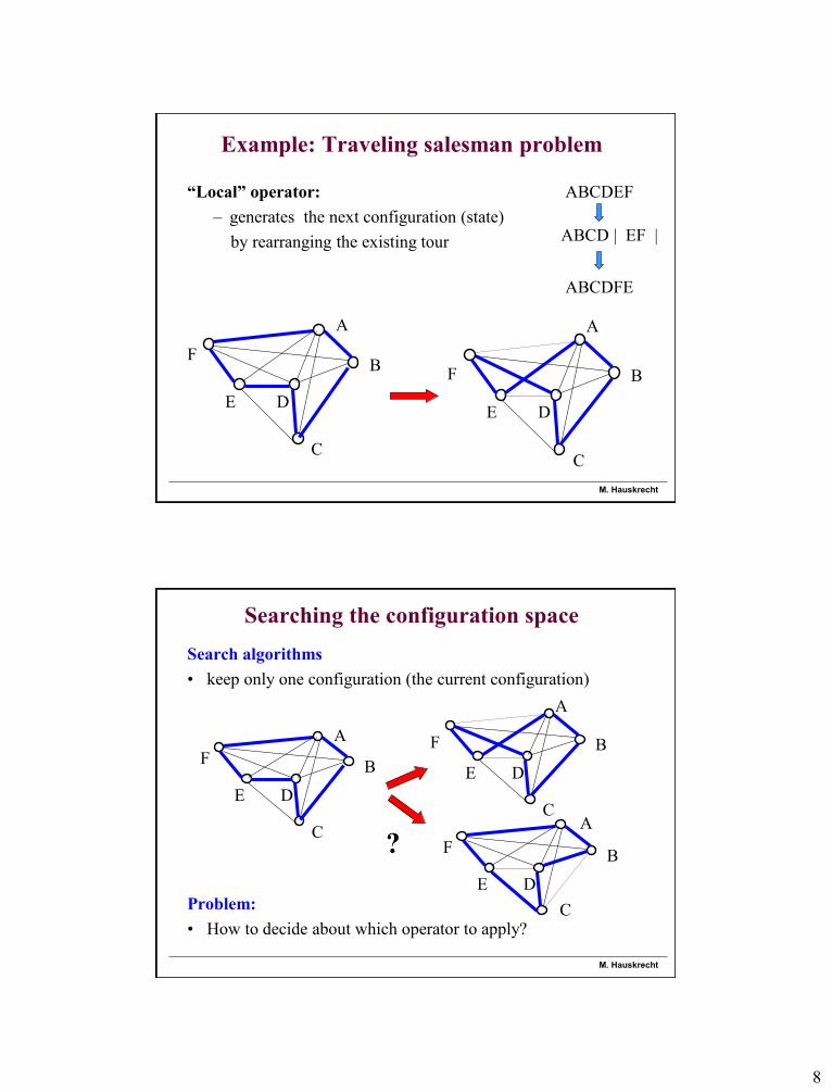
Example: Traveling salesman problem

“Local” operator:

– generates the next configuration (state)

by rearranging the existing tour

A

B

C

DE

F

A

B

C

DE

F

ABCD | EF |

ABCDFE

ABCDEF

M. Hauskrecht

Searching the configuration space

Search algorithms

• keep only one configuration (the current configuration)

Problem:

• How to decide about which operator to apply?

A

B

C

DE

FA

B

C

DE

F

A

B

DE

F

C

?

9

M. Hauskrecht

Search algorithms

Strategies to choose the configuration (state) to be visited

next:

– Hill climbing

– Simulated annealing

• Extensions to multiple current states:

– Genetic algorithms

• Note: Maximization is inverse of the minimization

)(max)(min sqsq

M. Hauskrecht

Hill climbing

• Only configurations one can reach using local moves are

consired as candidates

• What move the hill climbing makes?

value

states

I am currently here

A

B

C

D

E

F

10

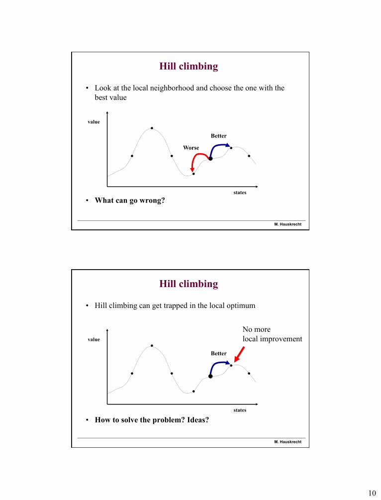
M. Hauskrecht

Hill climbing

• Look at the local neighborhood and choose the one with the

best value

• What can go wrong?

value

states

Better

Worse

M. Hauskrecht

Hill climbing

• Hill climbing can get trapped in the local optimum

• How to solve the problem? Ideas?

value

states

Better

No more

local improvement

11

M. Hauskrecht

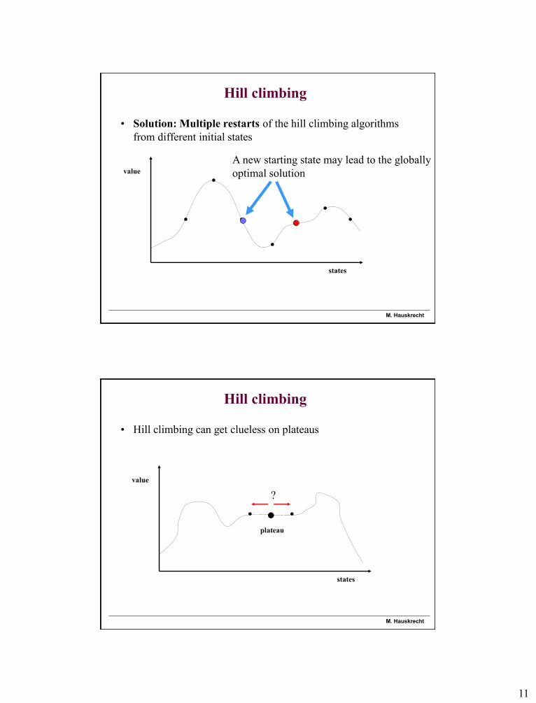
Hill climbing

• Solution: Multiple restarts of the hill climbing algorithms

from different initial states

value

states

A new starting state may lead to the globally

optimal solution

M. Hauskrecht

Hill climbing

• Hill climbing can get clueless on plateaus

value

states

plateau

?

12

M. Hauskrecht

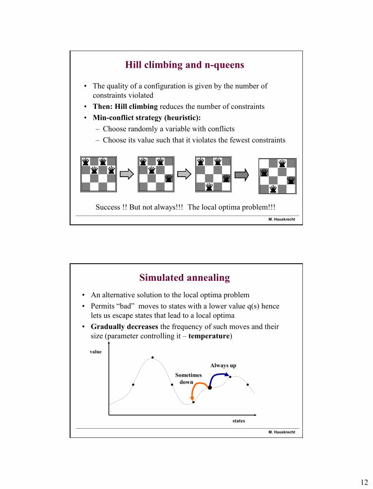
Hill climbing and n-queens

• The quality of a configuration is given by the number of

constraints violated

• Then: Hill climbing reduces the number of constraints

• Min-conflict strategy (heuristic):

– Choose randomly a variable with conflicts

– Choose its value such that it violates the fewest constraints

Success !! But not always!!! The local optima problem!!!

M. Hauskrecht

Simulated annealing

• An alternative solution to the local optima problem

• Permits “bad” moves to states with a lower value q(s) hence

lets us escape states that lead to a local optima

• Gradually decreases the frequency of such moves and their

size (parameter controlling it – temperature)

value

states

Always up

Sometimes

down

13

M. Hauskrecht

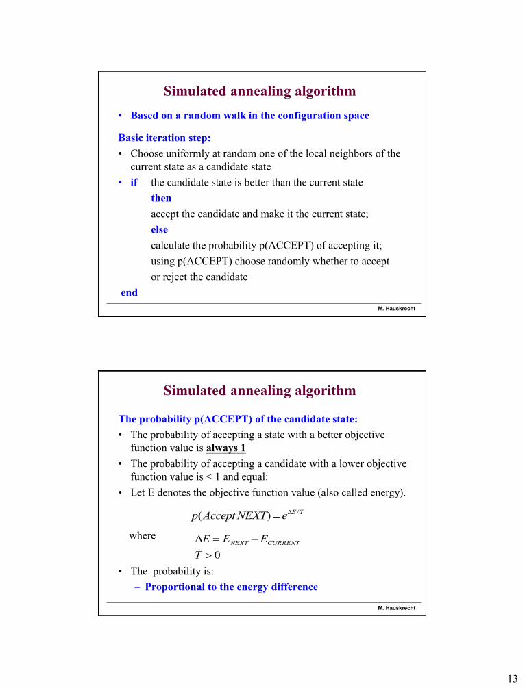
Simulated annealing algorithm

• Based on a random walk in the configuration space

Basic iteration step:

• Choose uniformly at random one of the local neighbors of the

current state as a candidate state

• if the candidate state is better than the current state

then

accept the candidate and make it the current state;

else

calculate the probability p(ACCEPT) of accepting it;

using p(ACCEPT) choose randomly whether to accept

or reject the candidate

end

M. Hauskrecht

Simulated annealing algorithm

The probability p(ACCEPT) of the candidate state:

• The probability of accepting a state with a better objective

function value is always 1

• The probability of accepting a candidate with a lower objective

function value is < 1 and equal:

• Let E denotes the objective function value (also called energy).

• The probability is:

– Proportional to the energy difference

TEeNEXTAcceptp /)(

0

T

EEE CURRENTNEXTwhere

14

M. Hauskrecht

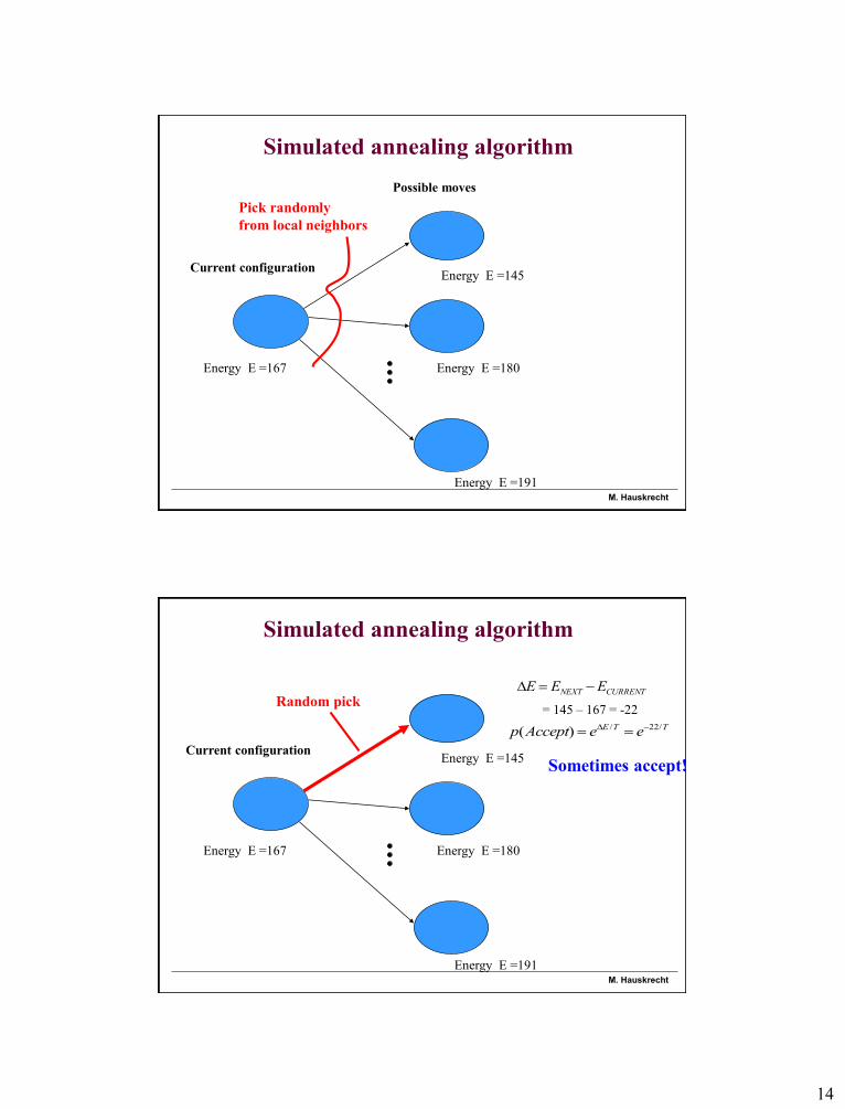
Simulated annealing algorithm

Current configuration

Energy E =167

Energy E =145

Energy E =180

Energy E =191

Possible moves

Pick randomly

from local neighbors

M. Hauskrecht

Simulated annealing algorithm

TTE eeAcceptp /22/)(

CURRENTNEXT EEE

Current configuration

Energy E =167

Energy E =145

Energy E =180

Energy E =191

= 145 – 167 = -22

Sometimes accept!

Random pick

15

M. Hauskrecht

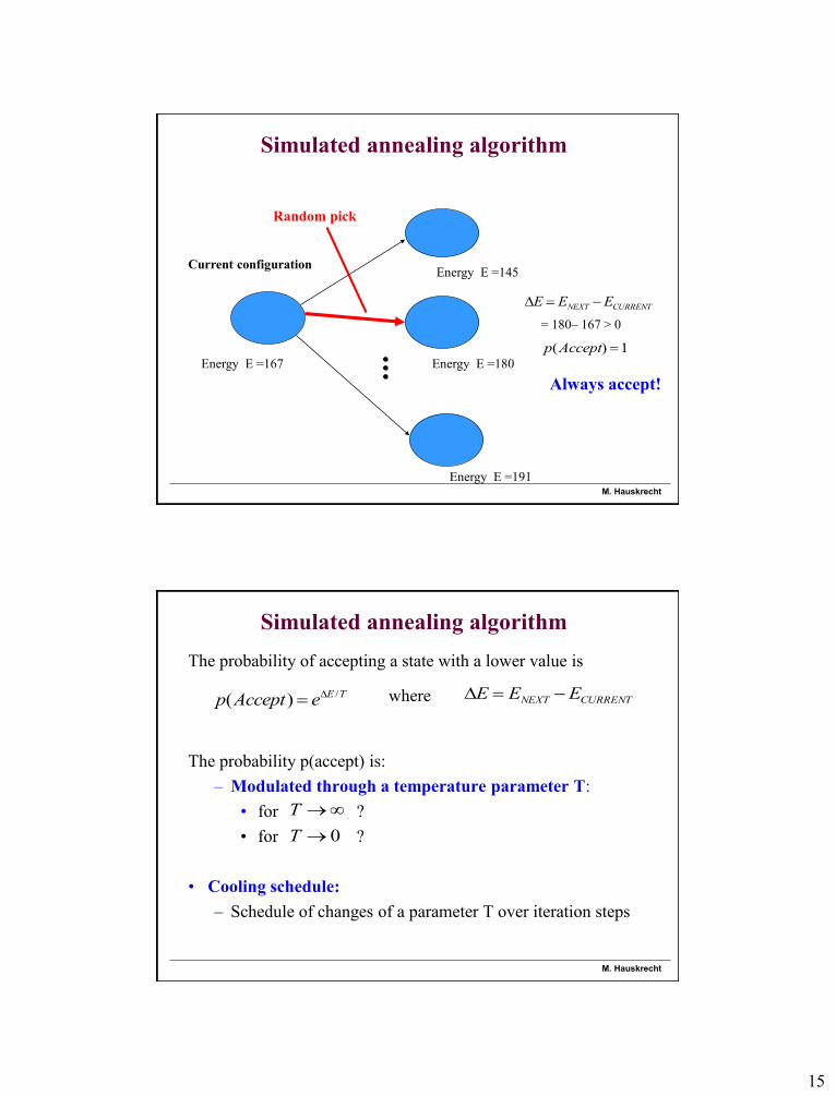
Simulated annealing algorithm

CURRENTNEXT EEE

Current configuration

Energy E =167

Energy E =145

Energy E =180

Energy E =191

= 180– 167 > 0

1)( Acceptp

Always accept!

Random pick

M. Hauskrecht

Simulated annealing algorithm

The probability of accepting a state with a lower value is

The probability p(accept) is:

– Modulated through a temperature parameter T:

• for ?

• for ?

• Cooling schedule:

– Schedule of changes of a parameter T over iteration steps

TEeAcceptp /)(

0T

CURRENTNEXT EEE

T

where

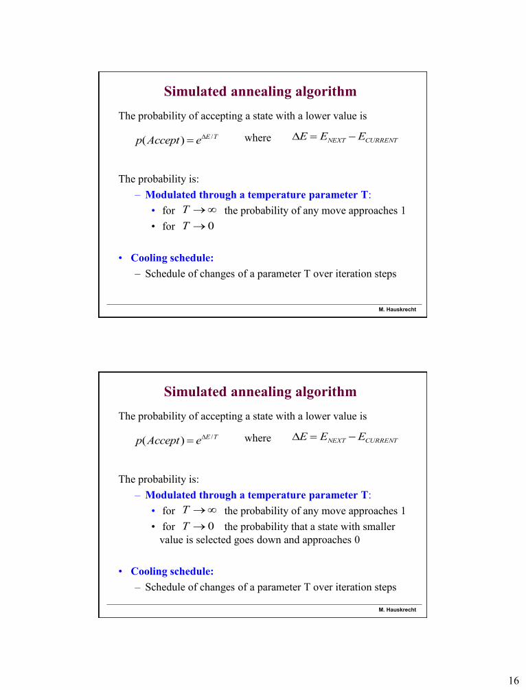
16

M. Hauskrecht

Simulated annealing algorithm

The probability of accepting a state with a lower value is

The probability is:

– Modulated through a temperature parameter T:

• for the probability of any move approaches 1

• for

• Cooling schedule:

– Schedule of changes of a parameter T over iteration steps

TEeAcceptp /)(

0T

CURRENTNEXT EEE

T

where

M. Hauskrecht

Simulated annealing algorithm

The probability of accepting a state with a lower value is

The probability is:

– Modulated through a temperature parameter T:

• for the probability of any move approaches 1

• for the probability that a state with smaller

value is selected goes down and approaches 0

• Cooling schedule:

– Schedule of changes of a parameter T over iteration steps

TEeAcceptp /)(

0T

CURRENTNEXT EEE

T

where

17

M. Hauskrecht

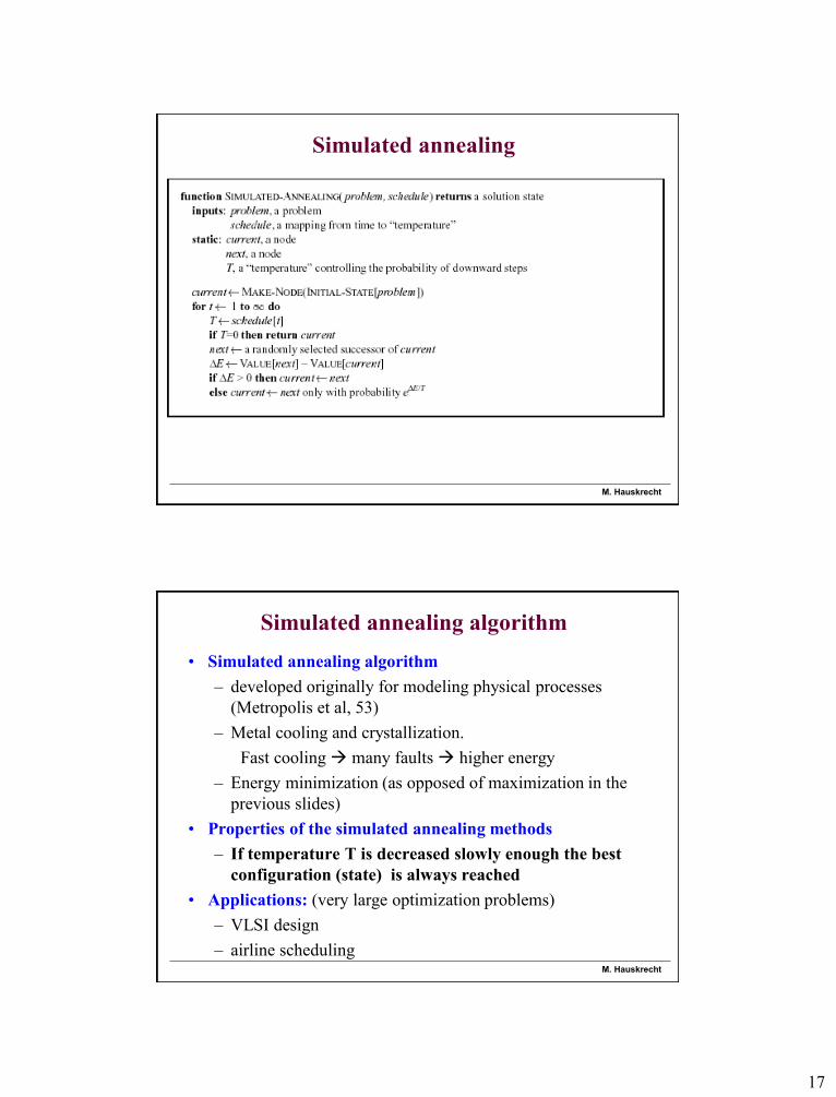
Simulated annealing

M. Hauskrecht

Simulated annealing algorithm

• Simulated annealing algorithm

– developed originally for modeling physical processes

(Metropolis et al, 53)

– Metal cooling and crystallization.

Fast cooling many faults higher energy

– Energy minimization (as opposed of maximization in the

previous slides)

• Properties of the simulated annealing methods

– If temperature T is decreased slowly enough the best

configuration (state) is always reached

• Applications: (very large optimization problems)

– VLSI design

– airline scheduling