Embed Size (px)
Citation preview

U.S. Department of the InteriorU.S. Geological Survey
Scientific Investigations Report 2021–5015
Methods for Estimating Regional Skewness of Annual Peak Flows in Parts of Eastern New York and Pennsylvania, Based on Data Through Water Year 2013

Methods for Estimating Regional Skewness of Annual Peak Flows in Parts of Eastern New York and Pennsylvania, Based on Data Through Water Year 2013
By Andrea G. Veilleux and Daniel M. Wagner
Scientific Investigations Report 2021–5015
U.S. Department of the InteriorU.S. Geological Survey

U.S. Geological Survey, Reston, Virginia: 2021
For more information on the USGS—the Federal source for science about the Earth, its natural and living resources, natural hazards, and the environment—visit https://www.usgs.gov or call 1–888–ASK–USGS.
For an overview of USGS information products, including maps, imagery, and publications, visit https://store.usgs.gov/.
Any use of trade, firm, or product names is for descriptive purposes only and does not imply endorsement by the U.S. Government.
Although this information product, for the most part, is in the public domain, it also may contain copyrighted materials as noted in the text. Permission to reproduce copyrighted items must be secured from the copyright owner.
Suggested citation:Veilleux, A.G., and Wagner, D.M., 2021, Methods for estimating regional skewness of annual peak flows in parts of eastern New York and Pennsylvania, based on data through water year 2013: U.S. Geological Survey Scientific Investigations Report 2021–5015, 38 p., https://doi.org/ 10.3133/ sir20215015.
Associated data for this publication:Wagner, D.M., and Veilleux, A.G., 2021, Regional flood skew for parts of the mid-Atlantic region (hydrologic unit 02) in eastern New York and Pennsylvania: U.S. Geological Survey data release, https://doi.org/10.5066/P9PGAL0D.
ISSN 2328-0328 (online)

iii
ContentsAbstract ...........................................................................................................................................................1Introduction.....................................................................................................................................................1
Purpose and Scope ..............................................................................................................................2Description of Study Area ...................................................................................................................2
Methods...........................................................................................................................................................5Streamgage Selection .........................................................................................................................5Redundancy Screening .......................................................................................................................5Basin Characteristics ...........................................................................................................................5Annual Exceedance Probability Analyses ........................................................................................6Bayesian Weighted Least Squares/Bayesian Generalized Least Squares Analysis ................6
Calculating Pseudo Record Length ..........................................................................................6Removing the Bias of the At-Site Estimators ..........................................................................8Estimating the Mean Square Error of the Skew ...................................................................11Developing a Cross-Correlation Model ..................................................................................11Regression Analyses .................................................................................................................13
Ordinary Least Squares Analysis ...................................................................................13Weighted Least Squares Analysis .................................................................................13Generalized Least Squares Analysis .............................................................................14
Results and Discussion ...............................................................................................................................15Final Bayesian Weighted Least Squares/Bayesian Generalized Least Squares Model ........15Bayesian Weighted Least Squares/Bayesian Generalized Least Squares Regression
Diagnostics .............................................................................................................................15Leverage and Influence .....................................................................................................................18
Summary........................................................................................................................................................20Acknowledgments .......................................................................................................................................20References Cited..........................................................................................................................................20Appendix 1. Assessment of a Regional Skew Model for Parts of Eastern New York and
Pennsylvania by Using Monte Carlo Simulations .....................................................................33
Figures
1. Maps of the study area in eastern New York and Pennsylvania ..........................................3 2. Map showing the pseudo record lengths (PRL) of streamgages that were used
in the regional skew analysis for parts of eastern New York and Pennsylvania ...............9 3. Map showing unbiased station skew of streamgages used in the regional skew
analysis for parts of eastern New York and Pennsylvania ..................................................10 4. Graphs showing cross correlation of annual peak flows in the study area .....................12 5. Map showing residuals from constant model of skew for 183 streamgages that
were used in the regional skew analysis for parts of eastern New York and Pennsylvania ...............................................................................................................................17

iv
Tables
1. Streamgages that were considered for use in the regional skew analysis for parts of eastern New York and Pennsylvania ..................................................26
2. Basin characteristics considered for use as explanatory variables in the regional skew analysis ................................................................................................................7
3. Regional skew model and model fit for parts of eastern New York and Pennsylvania ...............................................................................................................................15
4. Pseudo analysis of variance (pseudo ANOVA) table for the constant model of regional skew in parts of eastern New York and Pennsylvania .........................................16
5. Streamgages with high influence on the constant model of regional skew ....................19
Conversion FactorsInternational System of Units to U.S. customary units
Multiply By To obtain
Length
centimeter (cm) 0.3937 inch (in.)kilometer (km) 0.6214 mile (mi)
Volume
cubic meter (m3) 35.31 cubic foot (ft3)Flow rate
cubic meter per second (m3/s) 35.31 cubic foot per second (ft3/s)
DatumVertical coordinate information is referenced to the North American Vertical Datum of 1988 (NAVD 88).
Horizontal coordinate information is referenced to the North American Datum of 1983 (NAD 83).
v
AbbreviationsAEP annual exceedance probability
ASEV average sampling error variance
AVPnew average variance of prediction at a new streamgage
B17B Bulletin 17B (see Interagency Advisory Committee on Water Data, 1982)
B17C Bulletin 17C (see England and others, 2018)
B–GLS Bayesian generalized least squares
B–WLS Bayesian weighted least squares
DAR drainage area ratio
EMA expected moments algorithm
EVR error variance ratio
GAGES-II Geospatial Attributes of Gages for Evaluating Streamflow, Version II
GIS geographic information system
LP–III log-Pearson Type III distribution
MBV* misrepresentation of the beta variance
MGBT multiple Grubbs-Beck test
MSE mean square error
� �ˆMSE G mean squared error of skew
NWIS National Water Information System
OLS ordinary least squares
PILF potentially influential low flood
PRL pseudo record length
Pseudo ANOVA pseudo analysis of variance
SD standardized distance
USGS U.S. Geological Survey


Methods for Estimating Regional Skewness of Annual Peak Flows in Parts of Eastern New York and Pennsylvania, Based on Data Through Water Year 2013
By Andrea G. Veilleux and Daniel M. Wagner
AbstractBulletin 17C (B17C) recommends fitting the log-Pearson
Type III (LP−III) distribution to a series of annual peak flows at a streamgage by using the method of moments. The third moment, the skewness coefficient (or skew), is important because the magnitudes of annual exceedance probability (AEP) flows estimated by using the LP–III distribution are affected by the skew; interest is focused on the right-hand tail of the distribution, which represents the larger annual peak flows that correspond to small AEPs. For streamgages having modest record lengths, the skew is sensitive to extreme events like large floods, which cause a sample to be highly asymmet-rical or “skewed.” For this reason, B17C recommends using a weighted-average skew computed from the skew of the annual peak flows for a given streamgage and a regional skew. This report presents an estimate of regional skew for a study area encompassing parts of eastern New York and Pennsylvania. A total of 232 candidate U.S. Geological Survey streamgages that were unaffected by extensive regulation, diversion, urbanization, or channelization were considered for use in the skew analysis; after screening for redundancy and pseudo record length (PRL) of at least 36 years, 183 streamgages were selected for use in the study.
Flood frequencies for candidate streamgages were analyzed by employing the expected moments algorithm, which extends the method of moments so that it can accom-modate interval, censored, and historical/paleo flow data, as well as the multiple Grubbs-Beck test to identify potentially influential low floods in the data series. Bayesian weighted least squares/Bayesian generalized least squares regression was used to develop a regional skew model for the study area that would incorporate possible variables (basin character-istics) to explain the variation in skew in the study area. Ten basin characteristics were considered as possible explanatory variables; however, none produced a pseudo coefficient of determination (pseudo Rδ
2 ) greater than 1 percent; as a result, these characteristics did not help to explain the variation in skew in the study area. Therefore, a constant model that had a regional skew coefficient of 0.32 and an average variance of prediction at a new streamgage (AVPnew, which corresponds
to the mean square error [MSE] of 0.11) was selected. The AVPnew corresponds to an effective record length of 68 years, a marked improvement over the Bulletin 17B national skew map, whose reported MSE of 0.302 indicated a corresponding effective record length of only 17 years.
IntroductionFlood-frequency analysis of annual peak flows at
streamflow-gaging stations (hereafter referred to as “streamgages”) provides engineers, hydrologists, and many others estimates of the magnitudes and frequencies of floods for planning, design, and management of infrastructure along rivers and streams. The Subcommittee on Hydrology of the Federal Advisory Committee on Water Information recently published Bulletin 17C (herein referred to as “B17C”; England and others, 2018), which comprises updated guidelines for flood-frequency analysis. The bulletin recommends the use of the log-Pearson Type III (LP–III) distribution to fit a time series of annual peak flows measured by a streamgage to obtain estimates of flows corresponding to various annual exceedance probabilities (AEPs). In the case of flood-frequency analysis, the LP–III distribution is described by three moments: the mean, the standard deviation, and the skewness coefficient of the logarithms of the flows. The third moment, the skewness coefficient (hereafter referred to as the “skew”), is a measure of the asymmetry of the distribution as shown by the thicknesses of the tails of the distribution. In flood-frequency analysis, the skew is important because the magnitudes of AEP flows estimated by using the LP–III dis-tribution are affected by the skews of the annual peak flows at specific streamgages (hereafter referred to as “station skew”); interest is focused on the right-hand tail of the distribution, which represents annual peak flows corresponding to small AEPs of the larger flood flows.
For streamgages having modest record lengths, approxi-mately in the range of 25 to 100 years, the skew is sensitive to unusually large or small annual peak flows because they cause a sample of such flows to be asymmetrical or skewed (Griffis and Stedinger, 2007). Thus, B17C guidelines recommend

2 Methods for Estimating Regional Skewness of Annual Peak Flows in Parts of Eastern New York and Pennsylvania
using a weighted-average skew that is computed from the skew of the station’s annual peak flows and the regional skew. Using the weighted-average skew reduces the sensitivity of the station skew to extreme events, particularly for streamgages with short record lengths of less than approximately 25 years.
The B17C guidelines recommend using the Bayesian weighted least squares/Bayesian generalized least squares (B–WLS/B–GLS) method to estimate regional skew (England and others, 2018, p. 30). Using this procedure, the regional skew is estimated based on the station skew of the logarithms of annual peak-flow data. The B–WLS/B–GLS procedure first uses an ordinary least squares (OLS) regression analysis to generate an initial regional-skew model that is used to compute the variance of the station skew for each streamgage. Next, B–WLS is used to generate estimators of the regional skew model parameters. Finally, B–GLS is used to estimate the precision of the B–WLS parameter values, to estimate the model error variance and its precision, and to compute some diagnostic statistics. The expected moments algorithm (EMA; Cohn and others, 1997) is a generalization of the method-of-moments approach for flood-frequency analysis of annual peak flows from streamgages recommended by B17C. The B–WLS/B–GLS method can account for the complexities introduced by EMA and the cross correlation between annual peak flows at pairs of streamgages (Veilleux, 2011; Veilleux and others, 2011).
To date, the B–WLS/B–GLS method has been used to generate estimates of regional skew for several regions around the Nation (Parrett and others, 2011; Eash and others, 2013; Olson, 2014; Paretti and others, 2014; Southard and Veilleux, 2014; Curran and others, 2016; Mastin and others, 2016; Wagner and others, 2016; Veilleux and Wagner, 2019). In this study, the B–WLS/B–GLS procedure was used to estimate skew for a region encompassing parts of eastern New York and Pennsylvania (fig. 1) to improve estimates of regional skew and flows corresponding to various AEPs across the region.
Purpose and Scope
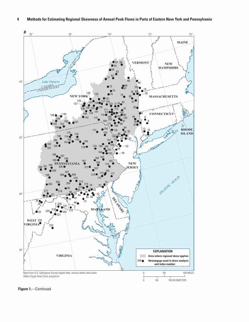
The purpose of this report is to present the results of a B–WLS/B–GLS analysis of regional skew for parts of eastern New York and Pennsylvania (fig. 1A). The scope of the project includes 183 streamgages in the Mid-Atlantic region (hydrologic units 0202, 0204, 0205, 0206, and 0207) and in the Connecticut Coastal region (hydrologic unit 0110) located in the States of Connecticut, Maryland, Massachusetts, New Jersey, New York, Pennsylvania, Vermont, Virginia, and West Virginia (fig. 1B). The number of available streamgages that
were unaffected by regulation or urbanization in hydrologic unit 0203 in southern New York and northern New Jersey (the Lower Hudson-Long Island region) was insufficient; therefore, the regional skew does not apply there. Flood-frequency analyses for the 183 streamgages were based on annual peak-flow data through water year 2013 (a water year is described as the period of October 1–September 30 and is named for the year in which it ends) and were performed using the U.S. Geological Survey (USGS) peak-flow analysis software (PeakFQ version 7.3; Veilleux and others, 2014; htt ps://water .usgs.gov/ software/ PeakFQ/ ). The results were used to analyze the regional skew.
A summary of information for each streamgage used in the regional skew analysis and a description of the basin characteristics considered as potential explanatory variables in the study are provided in the tables in this report. PeakFQ input files (.txt), PeakFQ setup files (.psf), PeakFQ output files (.PRT), a geographic information system (GIS) shapefile (con-taining streamgage information, basin characteristics, results of flood-frequency analysis, and B–WLS/B–GLS results), a comma-separated values file containing the attributes of the GIS shapefile, and the corresponding metadata are provided in a data release associated with this report (Wagner and Veilleux, 2021).
Description of Study Area
The study area encompasses part of the Mid-Atlantic region (hydrologic unit 02) and the Connecticut Coastal region (hydrologic unit 0110) and includes parts of the States of New York and Pennsylvania (fig. 1A). The study area encompasses 49,817 square miles and spans approximately 300 miles from north to south (from northern New York to the southern border of Pennsylvania) and approximately 200 miles from east to west (from west-central Pennsylvania to the eastern border of New York).
The study area is located entirely within the Appalachian Highlands physiographic division, which is characterized by hilly to mountainous terrain of the Adirondack, Valley and Ridge, Appalachian Plateaus, Piedmont, and New England physiographic provinces (Fenneman, 1938). Basin-averaged mean annual precipitation for streamgages in the study area ranged from 35 to 63 inches (88 to 160 centimeters; Falcone, 2011). Based on the 2011 National Land Cover Database, the study area is approximately 60 percent forested, 22 percent agricultural (crops and pasture), 10 percent developed, and 3 percent wetlands, with the remaining 5 percent including open water, barren land, shrub/scrub, and grassland/herbaceous categories (Homer and others, 2015).

Introduction 3
02050205
0202
0110
0203
02060207
0204
Lake Ontario
ATLANTIC O
CEAN
CANADA
UNITED STATES
A
Base from U.S. Geological Survey digital data, various dates and scalesAlbers Equal-Area Conic projection
0 100 KILOMETERS50
0 50 100 MILES
VIRGINIA
MARYLAND
WESTVIRGINIA
PENNSYLVANIA
NEW YORK
CONNECTICUT
NEWJERSEY
NEWHAMPSHIRE
MASSACHUSETTS
VERMONT
MAINE
DELAWARE
RHODEISLAND
76° 74° 72° 70°78°
38°
40°
42°
44°
Area where regional skew applies
4-digit hydrologic unit0205
EXPLANATION
Figure 1. Maps of the study area in eastern New York and Pennsylvania showing (A) 4-digit hydrologic units (U.S. Geological Survey, 2019), and (B) locations of the 183 streamgages used in the skew analysis.
4 Methods for Estimating Regional Skewness of Annual Peak Flows in Parts of Eastern New York and Pennsylvania
Lake Ontario
ATLANTIC O
CEAN
CANADA
UNITED STATES
B
Base from U.S. Geological Survey digital data, various dates and scalesAlbers Equal-Area Conic projection
0 100 KILOMETERS50
0 50 100 MILES
VIRGINIA
MARYLAND
WEST
VIRGINIA
PENNSYLVANIA
NEW YORK
CONNECTICUT
NEWJERSEY
NEWHAMPSHIRE
MASSACHUSETTS
VERMONT
MAINE
DELAWARE
RHODEISLAND
76° 74° 72° 70°78°
38°
40°
42°
44°
98
7
6
97
96
95
9492
91
90
89
8887
86
83
82 81
807978
77 76
75
7473
72
71
69
6867
6664
6362
6059
58
57
56
5554
5352
51
4847
46 45 44
43
4039
38
3736
3534
33
31
2827
2625
24
23
2221
2019
12
11
10
232
231230
229
228
227
222
221220
219
218
215
214213
212
217
211
210
209
208207
206
206
205
204202
200
199
198
197196
194193192191
190
189
188 187
186
185
183182
181180
179 178
177176175
174
173
172171
170168
167169
166165
164
163162
160161
159 158
157156
155154
152151150
149148
146145
144 142
141140
135137
136 138
134
133
131
130
128 127
126
125
124123
121
120
118
117
116115
111113
112
109
108
105104
102103
Area where regional skew applies
Streamgage used in skew analysisand index number
EXPLANATION
Figure 1.—Continued

Methods 5
Methods
Streamgage Selection
A suite of 232 candidate USGS streamgages were con-sidered for use in the regional skew analysis (table 1, which follows the “References Cited”). Annual peak flows for these streamgages were obtained from the USGS National Water Information System (NWIS; U.S. Geological Survey, 2018). Only streamgage records that were unaffected by extensive regulation, diversion, urbanization, or channelization (based on coding of annual peaks in the peak-flow files) and that had approximately 25 or more gaged peaks were considered for use in the regional skew analysis. Using these criteria, USGS employees who had local knowledge and experience in New York and Pennsylvania selected the candidate streamgages. A review of the study area boundary found that 17 streamgages were located outside the study area and were removed, after which 215 were left for use in the regional skew study (table 1). After that, streamgages that were deemed redundant were then screened and removed from the larger dataset (see the “Redundancy Screening” section for more information).
Redundancy Screening
Two streamgages may be redundant if their drainage basins are nested and similar in size; the drainage basins are considered nested if one entire drainage area is inside the other. If streamgages are redundant, a statistical analysis incorporating data from both streamgages incorrectly repre-sents the information content in the regional dataset (Gruber and Stedinger, 2008). Instead of providing two spatially independent observations that depict how the characteristics of each basin are related to skew, the basins will be assumed to exhibit similar hydrologic responses to a given storm and thus represent only one spatial observation. To determine whether two streamgages are redundant and thus represent the same watershed for the purposes of developing a regional hydro-logic model, two types of information are considered: (1) the standardized distance (SD) between the centroids of the basins and (2) the ratio of the drainage areas of the basins.
The SD between two basin centroids is used to deter-mine the likelihood that the basins are redundant. The SD is defined as
SDD
DRNAREA DRNAREAij
ij
i j
��� �0 5.
, (1)
where Dij is the distance between centroids of basin i
and basin j, in miles; DRNAREAi is the drainage area at streamgage i, in
square miles; and DRNAREAj is the drainage area at streamgage j, in
square miles.
The drainage area ratio (DAR) is used to determine if two nested basins are sufficiently similar in size that they represent the same watershed for the purposes of developing a regional hydrologic model (Veilleux, 2009). The DAR is defined as
DAR MaxDRNAREADRNAREA
DRNAREADRNAREA
i
j
j
i
��
���
�
���
, , (2)
where DAR is the Max (maximum) of the two values in
brackets, DRNAREAi is the drainage area at streamgage i, and DRNAREAj is the drainage area at streamgage j.
Streamgage pairs having a SD less than or equal to 0.50 and a DAR less than or equal to 5.0 are likely to be redundant for purposes of determining regional skew (Veilleux, 2009). If the DAR is large enough, even nested streamgages will reflect different hydrologic responses because storms of different sizes and durations typically affect sites differently.
All possible combinations of streamgage pairs from the 215 streamgages were considered in the redundancy analysis. All streamgage pairs with a SD ≤ 0.5 and a DAR ≤ 5.0 were identified as possibly redundant. The drainage area of each streamgage was then investigated to determine if one of the two drainage areas was nested inside the other; if this was true, the preference was generally for the streamgage that had the smaller drainage area and the longer record length. The procedure identified 24 possibly redundant streamgage pairs; of these, 17 streamgages were found to be redundant and were removed from the analysis.
Basin Characteristics
Basin characteristics for the streamgages used in the skew analysis were either obtained from the USGS Geospatial Attributes of Gages for Evaluating Streamflow, Version II (GAGES-II) database or were generated. The GAGES-II database consists of a subset of USGS streamgages that have at least 20 years of streamflow record since 1950 or that were active as of water year 2009 and whose watersheds lie within the United States (Falcone, 2011). For streamgages that were used in the skew analysis but were not in the GAGES-II database, the suite of basin characteristics was generated by using the ArcHydro package in Esri ArcGIS software version 10.3.1 (Environmental Systems Research Institute, 2009; Eash and others, 2013; Wagner and others, 2016). This procedure ensured that a consistent suite of basin characteristics was available for all of the streamgages used in the skew analysis.
Basin characteristics were selected to potentially explain the variation in skew in the study area. These included morphometric (drainage area, latitude and longitude of basin centroid, mean basin slope, mean basin elevation, and basin compactness ratio), climatological (basin-average mean annual
6 Methods for Estimating Regional Skewness of Annual Peak Flows in Parts of Eastern New York and Pennsylvania
precipitation), and pedologic or geologic (areal percentages of open water and forest, and average soil permeability) characteristics (table 2).
Annual Exceedance Probability Analyses
To estimate regional skew for parts of eastern New York and Pennsylvania, a flood-frequency analysis must first be conducted for each streamgage to determine the station skew and its associated mean square error (MSE). The B17C guide-lines recommend fitting the LP–III distribution to a series of annual peak flows at a streamgage by using the method of moments (England and others, 2018). In doing so, it is recommended that EMA is employed to extend the method of moments to accommodate interval, censored, and historical or paleo flood data, as well as the use of the multiple Grubbs-Beck test (MGBT) to identify potentially influential low floods (PILFs) in the data series. In this study, the USGS software PeakFQ version 7.3 was used to analyze the flood frequencies (Veilleux and others, 2014).
Hydrologists in the USGS Water Science Centers in New York and Pennsylvania used EMA with PeakFQ version 7.3 for candidate streamgages in their States and for candi-date streamgages in the surrounding states of Connecticut, Maryland, Massachusetts, New Jersey, Vermont, Virginia, and West Virginia. Flood frequencies were analyzed by using the station-skew option in PeakFQ software and, with few exceptions (such as a fixed threshold for PILFs that yielded a superior fit of the flood-frequency model to the dataset), the MGBT for PILFs. Historical peaks were included in the analy-sis; annual peak flows coded as urban or regulated were not. Hydrologists in New York and Pennsylvania assigned percep-tion thresholds to each period of record (including historical and missing periods as well as periods of crest-stage gage operation) and assigned flow intervals to uncertain annual peak flows as appropriate.
Bayesian Weighted Least Squares/Bayesian Generalized Least Squares Analysis
Prior to analyzing regional skew by the B–WLS/B–GLS method, three preliminary steps were completed: (1) calcula-tion of the pseudo record length for each streamgage, given the number of censored observations and concurrent record lengths; (2) removal of structural bias in the estimate of station skew and its MSE; and (3) development of a cross-correlation model of concurrent annual peak flows between streamgages.
Calculating Pseudo Record Length
The pseudo record length of the annual peak-flow series at each streamgage is used in the regional skew study in sev-eral steps, including unbiasing the station skew and its mean square error, determining the concurrent record length between
two streamgages, and computing the cross correlation of the station skews. Because the dataset includes censored data and historical information, the effective record length used to compute the precision of the skewness estimators is no longer simply the number of annual peak flows at a streamgage. Instead, a more complex calculation based on the availability of historical information and censored values is used. Whereas historical information and records of censored peaks provide valuable information, they often provide less information than records of an equal number of years of gaged peaks (Stedinger and Cohn, 1986). The calculations described in the following paragraphs yield a pseudo record length (PRL) associated with skew, which appropriately accounts for all types of peak-flow data available from a streamgage. If no interval, censored, and (or) historical data are present in the annual peak-flow record of a streamgage, PRL is equal to the gaged record length.
The PRL is defined as the number of years of gaged record that would be required to yield the same mean squared error of the skew ( � �ˆMSE G ) as would the combination of the historical and gaged records that are actually available at a streamgage. Thus, the PRL of the skew is a ratio of the MSE of the station skew when only the gaged record is analyzed ( � �ˆ
SMSE G ) to the MSE of the station skew when the entire record, including historical and censored data, is analyzed ( � �ˆ
CMSE G ):
� �
� �ˆ
ˆs S
RL
C
P MSE GP
MSE G
�� , (3)
where PRL is the pseudo length of the entire record at the
streamgage, in years; Ps is the number of years with gaged peaks in
the record; � �ˆ
SMSE G is the estimated MSE of the skew when only the gaged record is analyzed; and
� �ˆCMSE G is the estimated MSE of the skew when the
entire record, including historical and censored data, is analyzed.
Because the PRL is an estimate, the following conditions must also be met to ensure a valid approximation. The PRL must be nonnegative. If PRL is greater than PH (the length of the historical period), then PRL should be set to equal PH. Also, if PRL is less than PS, then PRL is set to PS. This ensures that the PRL will not be larger than the complete PH or less than PS.
As stated in B17C, the station skew is sensitive to extreme events; therefore, accurate estimates of skew require longer periods of record, typically 50 years or greater. However, 50 years of record are not available for most streamgages, and therefore a minimum of 30 to 40 years has been used in recent studies (Eash and others, 2013; Paretti and

Methods
7
Table 2. Basin characteristics considered for use as explanatory variables in the regional skew analysis.
[GIS, geographic information system; NHDPlus, National Hydrography Dataset Plus; NAD83, North American Datum of 1983; PRISM, Parameter Regression on Independent Slopes Model; NLCD, National Land Cover Database]
Basin characteristic Units Source
Drainage area of streamgage basin, delineated by using GIS
Square kilometers Derived from 30-meter NHDPlus data, http://www.horizon- systems.com/ nhdplus/ .
Latitude of basin centroid Decimal degrees, NAD83 Determined from zonal statistics of grids derived from basin polygons in Esri ArcGIS, version 10.3.1.
Longitude of basin centroid Decimal degrees, NAD83 Determined from zonal statistics of grids derived from basin polygons in Esri ArcGIS, version 10.3.1.
Mean basin elevation Meters Determined from 10-meter resolution National Elevation Dataset, https://www .usgs.gov/ core- science- systems/ national- geospatial- program/ national- map.
Basin compactness ratio (area/perimeter2×100); higher number indicates more compact shape
Unitless Calculated in Esri ArcGIS, version 10.3.1, by using drainage area and perimeter of GIS-delineated basin polygons.
Basin-averaged mean annual precipitation for the 30-year period of 1971 to 2000
Centimeters 800-meter PRISM data, Oregon State University, htt p://www.pr ism.oregon state.edu/ .
Mean basin slope Percent Determined from 100-meter resolution National Elevation Dataset, https://www .usgs.gov/ core- science- systems/ national- geospatial- program/ national- map.
Basin-averaged soil permeability Inches per hour Wolock (1997, htt ps://water .usgs.gov/ GIS/ metadata/ usgswrd/ XML/ muid.xml) and U.S. Department of Agriculture (2008, https://websoilsurvey.sc.egov.usda.gov/App/WebSoilSurvey.aspx).
Percentage of streamgage basin in forested land-use categories
Percentage of streamgage basin surface area 2006 NLCD, sum of classes 41, 42, and 43, h ttps://www .mrlc.gov/ data? f%5B0%5D= year%3A2006.
Percentage of streamgage basin in open water Percentage of streamgage basin surface area 2006 NLCD, class 11, h ttps://www .mrlc.gov/ data? f%5B0%5D= year%3A2006.
8 Methods for Estimating Regional Skewness of Annual Peak Flows in Parts of Eastern New York and Pennsylvania
others, 2014; Southard and Veilleux, 2014; Wagner and others, 2016). Thus, after adequate geographic and hydrologic coverage was ensured, streamgages in the dataset that had a PRL less than 36 years were removed from the study. Of the 198 streamgages that remained after removing the 17 streamgages located outside the study area boundary and the 17 redundant streamgages, an additional 15 were removed for having a PRL less than 36 years, leaving 183 streamgages from which a regional skew model was developed (table 1; fig. 2).
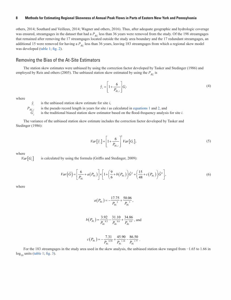
Removing the Bias of the At-Site EstimatorsThe station skew estimates were unbiased by using the correction factor developed by Tasker and Stedinger (1986) and
employed by Reis and others (2005). The unbiased station skew estimated by using the PRL is
,
ˆ 61i iRL i
GP
γ� �
� �� �� �� �
, (4)
where ˆiγ is the unbiased station skew estimate for site i, PRL,i is the pseudo record length in years for site i as calculated in equations 1 and 2, and Gi is the traditional biased station skew estimator based on the flood-frequency analysis for site i.
The variance of the unbiased station skew estimate includes the correction factor developed by Tasker and Stedinger (1986):
� � � �2
,
61ˆi iRL i
Var Var GP
γ� �
� �� �� �� �
, (5)
where Var Gi� � is calculated by using the formula (Griffis and Stedinger, 2009):
� � � � � � � �2 46 9 151 ˆ6 48
ˆ ˆRL RL RL
RL
Var G a P b P G c P GP� � � �� � � �� � � � � � �� � � � � �� �� � � �� �� �
, (6)
where
a PP PRLRL RL
� � � � �17 75 50 06
2 3
. . ,
b PP P PRLRL RL RL
� � � � �3 92 31 10 34 86
0 3 0 6 0 9
. . .
. . ., and
c PP P PRLRL RL RL
� � � � � �7 31 45 90 86 50
0 59 1 18 1 77
. . .
. . . .
For the 183 streamgages in the study area used in the skew analysis, the unbiased station skew ranged from −1.65 to 1.66 in log10 units (table 1; fig. 3).

Methods 9
Lake Ontario
ATLANTIC O
CEAN
CANADA
UNITED STATES
Base from U.S. Geological Survey digital data, various dates and scalesAlbers Equal-Area Conic projection
0 100 KILOMETERS50
0 50 100 MILES
VIRGINIA
MARYLAND
WESTVIRGINIA
PENNSYLVANIA
NEW YORK
CONNECTICUT
NEWJERSEY
NEWHAMPSHIRE
MASSACHUSETTS
VERMONT
MAINE
DELAWARE
RHODEISLAND
76° 74° 72° 70°78°
38°
40°
42°
44°
Area where regional skew applies
Pseudo record length (PRL) ofstreamgage, in years
36 to 50
51 to 70
71 to 90
91 to 127
EXPLANATION
Figure 2. Map showing the pseudo record lengths (PRL) of streamgages that were used in the regional skew analysis for parts of eastern New York and Pennsylvania.

10 Methods for Estimating Regional Skewness of Annual Peak Flows in Parts of Eastern New York and Pennsylvania
Lake Ontario
ATLANTIC O
CEAN
CANADA
UNITED STATES
Base from U.S. Geological Survey digital data, various dates and scalesAlbers Equal-Area Conic projection
0 100 KILOMETERS50
0 50 100 MILES
VIRGINIA
MARYLAND
WESTVIRGINIA
PENNSYLVANIA
NEW YORK
CONNECTICUT
NEWJERSEY
NEWHAMPSHIRE
MASSACHUSETTS
VERMONT
MAINE
DELAWARE
RHODEISLAND
38°
40°
42°
44°
76° 74° 72° 70°78°
Area where regional skew applies
Unbiased skew of streamgage, inlog10 units
–1.65 to –0.75
–0.74 to –0.25
–0.24 to 0.25
0.26 to 0.75
0.76 to 1.66
EXPLANATION
Figure 3. Map showing unbiased station skew of streamgages used in the regional skew analysis for parts of eastern New York and Pennsylvania.
Methods 11
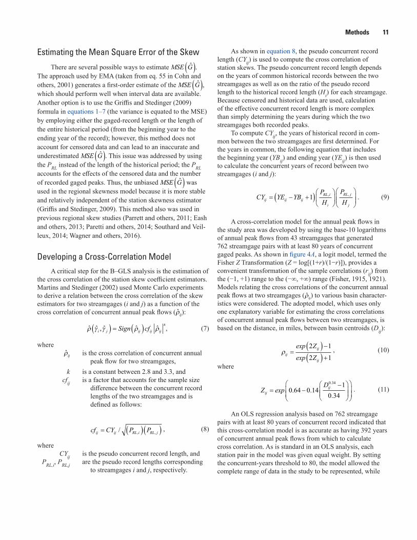
Estimating the Mean Square Error of the Skew
There are several possible ways to estimate � �ˆMSE G . The approach used by EMA (taken from eq. 55 in Cohn and others, 2001) generates a first-order estimate of the � �ˆMSE G , which should perform well when interval data are available. Another option is to use the Griffis and Stedinger (2009) formula in equations 1–7 (the variance is equated to the MSE) by employing either the gaged-record length or the length of the entire historical period (from the beginning year to the ending year of the record); however, this method does not account for censored data and can lead to an inaccurate and underestimated � �ˆMSE G . This issue was addressed by using the PRL instead of the length of the historical period; the PRL accounts for the effects of the censored data and the number of recorded gaged peaks. Thus, the unbiased � �ˆMSE G was used in the regional skewness model because it is more stable and relatively independent of the station skewness estimator (Griffis and Stedinger, 2009). This method also was used in previous regional skew studies (Parrett and others, 2011; Eash and others, 2013; Paretti and others, 2014; Southard and Veil-leux, 2014; Wagner and others, 2016).
Developing a Cross-Correlation ModelA critical step for the B–GLS analysis is the estimation of
the cross correlation of the station skew coefficient estimators. Martins and Stedinger (2002) used Monte Carlo experiments to derive a relation between the cross correlation of the skew estimators for two streamgages (i and j) as a function of the cross correlation of concurrent annual peak flows ( ˆ ijρ ):
� � � �ˆ ˆ ˆˆ ˆ,k
i j ij ij ijSign cfρ γ γ ρ ρ� , (7)
where ˆ ijρ is the cross correlation of concurrent annual
peak flow for two streamgages, k is a constant between 2.8 and 3.3, and cfij is a factor that accounts for the sample size
difference between the concurrent record lengths of the two streamgages and is defined as follows:
cf CY P Pij ij RL i RL j� � �� �/, ,
, (8)
where CYij is the pseudo concurrent record length, and PRL,i, PRL,j are the pseudo record lengths corresponding
to streamgages i and j, respectively.
As shown in equation 8, the pseudo concurrent record length (CYij) is used to compute the cross correlation of station skews. The pseudo concurrent record length depends on the years of common historical records between the two streamgages as well as on the ratio of the pseudo record length to the historical record length (Hi) for each streamgage. Because censored and historical data are used, calculation of the effective concurrent record length is more complex than simply determining the years during which the two streamgages both recorded peaks.
To compute CYij, the years of historical record in com-mon between the two streamgages are first determined. For the years in common, the following equation that includes the beginning year (YBij) and ending year (YEij) is then used to calculate the concurrent years of record between two streamgages (i and j):
CY YE YBPH
PHij ij ij
RL i
i
RL j
j
� � �� ����
�
���
���
�
���1
, , . (9)
A cross-correlation model for the annual peak flows in the study area was developed by using the base-10 logarithms of annual peak flows from 43 streamgages that generated 762 streamgage pairs with at least 80 years of concurrent gaged peaks. As shown in figure 4A, a logit model, termed the Fisher Z Transformation (Z = log[(1+r)/(1−r)]), provides a convenient transformation of the sample correlations (rij) from the (−1, +1) range to the (−∞, +∞) range (Fisher, 1915, 1921). Models relating the cross correlations of the concurrent annual peak flows at two streamgages ( ˆ ijρ ) to various basin character-istics were considered. The adopted model, which uses only one explanatory variable for estimating the cross correlations of concurrent annual peak flows between two streamgages, is based on the distance, in miles, between basin centroids (Dij):
�ijij
ij
exp Z
exp Z�
� � �� � �2 1
2 1
, (10)
where
Z expD
ijij� �
��
���
�
���
�
���
�
���
0 64 0 141
0 34
0 34
. ..
.
. (11)
An OLS regression analysis based on 762 streamgage pairs with at least 80 years of concurrent record indicated that this cross-correlation model is as accurate as having 392 years of concurrent annual peak flows from which to calculate cross correlation. As is standard in an OLS analysis, each station pair in the model was given equal weight. By setting the concurrent-years threshold to 80, the model allowed the complete range of data in the study to be represented, while

12 Methods for Estimating Regional Skewness of Annual Peak Flows in Parts of Eastern New York and Pennsylvania
res20-0073_fig4
0 100 200 300 400 500−0.25
0
0.25
0.5
0.75
1
1.25
1.5
Distance between basin centroids, in miles
Fish
er Z
-tran
sfor
med
cro
ss c
orre
latio
n of
ann
ual p
eak
flow
s fo
rst
ream
gage
pai
rs w
ith a
t lea
st 8
0 ye
ars
of c
oncu
rren
t rec
ord
0 100 200 300 400 500
−0.2
−0.3
−0.1
0
0.2
0.3
0.1
0.4
0.5
0.8
0.9
0.6
0.7
1
Distance between basin centroids, in miles
Untra
nsfo
rmed
cro
ss c
orre
latio
n of
ann
ual p
eak
flow
s fo
rst
ream
gage
pai
rs w
ith a
t lea
st 8
0 ye
ars
of c
oncu
rren
t rec
ord
EXPLANATION
Streamgage pairs
r = (exp(2Z )−1)/(exp(2Z )+1)
B
EXPLANATION
Streamgage pairs
Z = exp[0.64 + −0.14((D 0.34−1)/0.34)]
A
Figure 4. Graphs showing cross correlation of annual peak flows in the study area. A, Relation between Fisher Z-transformed cross correlation of logarithms of annual peak flows and the distances between basin centroids for 762 streamgage pairs with at least 80 years of concurrent record. B, Relation between untransformed cross correlation of logarithms of annual peak flows and the distances between basin centroids for 762 streamgage pairs with at least 80 years of concurrent record. Abbreviations: r, cross correlation of concurrent annual peak flows; D, distance between basin centroids, in miles; and Z, Fisher Z-transformed cross correlation of annual peak flows.

Methods 13
also minimizing the influence of station pairs with less accuracy and (or) less data. The fitted OLS regression relation between Z and the distance between basin centroids from the 762 streamgage pairs (fig. 4A) shows an exponential decline in the cross cor-relation for streamgages within 100 miles of each other. A similar decline is found in the cross correlation and distance between basin centroids for the untransformed streamgage pairs (fig. 4B). This model was used to estimate cross correlation for concur-rent annual peak flows between all streamgage pairs used in the regional skew study.
Regression AnalysesThe B–WLS/B–GLS method for computing a regional skew begins with an OLS analysis to develop a regional skew model
that is used to generate an estimate of regional skew for each streamgage (Veilleux, 2011; Veilleux and others, 2011, 2012). The OLS-based regional skew estimate is the basis for computing the variance of the skew for each streamgage. Next, B–WLS is used to generate estimators of the regional skew model parameters. Finally, B–GLS is used to estimate the precision of the B–WLS parameter values and the model error variance and its precision, and to compute various diagnostic statistics.
Ordinary Least Squares AnalysisThe first step in the B–WLS/B–GLS regional skew analysis is to prepare an initial regional skew model by using OLS
regression. The OLS regression analysis yields parameters (such as ˆOLSβ ) and a model that can be used to generate unbiased
regional estimates of the skew for all streamgages:
ˆOLS OLSy �� Xβ , (12)
where yOLS are the estimated regional skew values, X is a (n × k) matrix of basin characteristics, ˆ
OLSβ is a (k × 1) vector of estimated regression parameters, n is the number of streamgages, and k is the number of basin parameters, including a column of ones, to estimate the regression constant.
The estimated regional skew values ( yOLS) are then used to calculate unbiased streamgage regional skew variances by using equation 8 in Griffis and Stedinger (2009). These variances are based on the OLS estimator of the regional skew coef-ficient instead of the station skew estimator, making the weights in the subsequent steps relatively independent of the station skew estimates.
Weighted Least Squares AnalysisA B–WLS analysis is used to develop estimators of the regression coefficients for the regional skew model. The B–WLS
analysis explicitly reflects variations in record length but intentionally neglects cross correlations, thereby avoiding problems experienced with B–GLS parameter estimators (Veilleux, 2011; Veilleux and others, 2011).
The first step in the B–WLS analysis is to estimate the model error variance (�� ,B WLS�2 ) (Reis and others, 2005). Using a
B–WLS approach to estimate the model error variance precludes the pitfall of estimating the model error variance as zero, which can occur when the method-of-moments weighted least-squares regression is used. Although the B–WLS analysis produces an estimate of the distribution of the model error variance, only the mean model error variance estimator is considered. Given the model error variance estimator, a B–WLS analysis is used to generate the weight matrix (W) needed to compute estimates of the final regression parameters ( ˆ
B WLS�β ). To compute W, a diagonal covariance matrix [ɅB WLS B WLS,2 ] is created (eq. 13). The
diagonal elements of the covariance matrix are the sum of the estimated model error variance and the variance of the unbiased station skew ( � �ˆiVar γ ), which depends upon the record length and the estimate of the previously calculated OLS regional skew ( yOLS). The off-diagonal elements of ɅB WLS B WLS,
2 are zero because cross correlations among sets of streamgage data are not considered in the B–WLS analysis. Thus, the (n × n) covariance matrix, ɅB WLS B WLS,
2 , is given by
� � � �� �2 2, , ˆB WLS B WLS B WLS diag Varδ δσ σ� �� � �Λ I γ , (13)
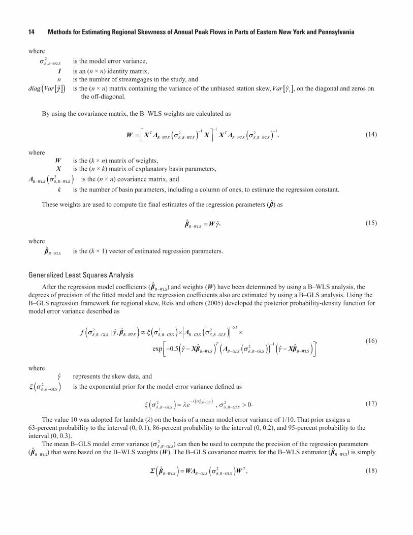
14 Methods for Estimating Regional Skewness of Annual Peak Flows in Parts of Eastern New York and Pennsylvania
where �� ,B WLS�
2 is the model error variance, I is an (n × n) identity matrix, n is the number of streamgages in the study, and � �� �ˆdiag Var γ is the (n × n) matrix containing the variance of the unbiased station skew, � �ˆiVar γ , on the diagonal and zeros on
the off-diagonal.
By using the covariance matrix, the B–WLS weights are calculated as
� � � �11 12 2
, ,T T
B WLS B WLS B WLS B WLSδ δσ σ�� �
� �� �� �� � �� �
W X Λ X X Λ , (14)
where W is the (k × n) matrix of weights, X is the (n × k) matrix of explanatory basin parameters, � �2
,B WLS B WLSδσ ��Λ is the (n × n) covariance matrix, and k is the number of basin parameters, including a column of ones, to estimate the regression constant.
These weights are used to compute the final estimates of the regression parameters (β̂) as
ˆ ˆB WLS γ� �β W , (15)
where ˆ
B WLS�β is the (k × 1) vector of estimated regression parameters.
Generalized Least Squares AnalysisAfter the regression model coefficients ( ˆ
B WLS�β ) and weights (W) have been determined by using a B–WLS analysis, the degrees of precision of the fitted model and the regression coefficients also are estimated by using a B–GLS analysis. Using the B–GLS regression framework for regional skew, Reis and others (2005) developed the posterior probability-density function for model error variance described as
� � � � � �
� � � �� � � �
0.52 2 2, , ,
12,
ˆˆ| ,
ˆ ˆˆ ˆ exp 0.5
B GLS B WLS B GLS B GLS B GLS
T
B WLS B GLS B GLS B WLS
f δ δ δ
δ
σ γ ξ σ σ
γ σ γ
�
� � � � �
�
� � � �
� � �
� �� � �� �� �
β Λ
Xβ Λ Xβ, (16)
where γ̂ represents the skew data, and � �� ,B GLS�� �2 is the exponential prior for the model error variance defined as
, ,
,
B GLS B GLSe B GLS2 22
0. (17)
The value 10 was adopted for lambda (λ) on the basis of a mean model error variance of 1/10. That prior assigns a 63-percent probability to the interval (0, 0.1), 86-percent probability to the interval (0, 0.2), and 95-percent probability to the interval (0, 0.3).
The mean B–GLS model error variance (�� ,B GLS�2 ) can then be used to compute the precision of the regression parameters
( ˆB WLS�β ) that were based on the B–WLS weights (W). The B–GLS covariance matrix for the B–WLS estimator ( ˆ
B WLS�β ) is simply
� � � �2,
ˆ TB WLS B GLS B GLSδσ� � ��Σ β WΛ W , (18)

Results and Discussion 15
where W is the (k × n) matrix of weights determined by
B–WLS analysis, WT is the transformation of W, and
� �2,B GLS B GLSδσ� �Λ is the (n × n) B–GLS covariance matrix
calculated as
� � � �2 2, , ˆB GLS B GLS B GLSδ δσ σ� � �� �Λ I Σ γ , (19)
where I is an (n × n) identity matrix, and � �ˆΣ γ is a full (n × n) matrix containing the
sampling variances of the streamflow record’s unbiased skew, � �ˆiVar γ , and the covariances of the skew ˆiγ .
The off-diagonal values of � �ˆΣ γ are determined by the cross correlation of concurrent gaged annual peak flows and the cf factor (see eq. 8), which accounts for the size differences between pairs of samples collected at different streamgages and their concurrent record length (Martins and Stedinger, 2002). In the calculation of the cf factor, only the gaged records and historical peaks are considered when determining the ratio of the number of concurrent peak flows at streamgage pairs to the total number of annual peak flows at both streamgages. Thus, any additional information pro-vided by perception thresholds and censored peaks in the EMA analysis is neglected in the calculation of the cross correlation of annual peak flows and the cf factor. Precision metrics include (1) the standard error of the regression param-eters [ � �ˆ
B WLSSE �β ]; (2) the model error variance (�� ,B GLS�2 );
(3) pseudo coefficient of determination (pseudo Rδ2); and
(4) the average variance of prediction at a new streamgage not used in the regional model (AVPnew).
Results and Discussion
Final Bayesian Weighted Least Squares/Bayesian Generalized Least Squares Model
A constant B–WLS/B–GLS model (having a skew of 0.32 and developed by using data from 183 streamgages with at least 36 years of PRL each) produced the only statistically
significant model of skew in the study area (table 3). A con-stant model does not explain any variability in skew; there-fore, the pseudo Rδ
2, a diagnostic statistic that describes the percentage of the variability in the skew from streamgage to streamgage that is estimated by the model (Gruber and others, 2007; Parrett and others, 2011), is 0 percent. All available basin characteristics were evaluated as possible explanatory variables in the B–WLS/B–GLS regression analysis; however, the addition of any of the available basin characteristics or combinations thereof did not produce a pseudo Rδ
2 greater than 1 percent, indicating that they did not explain the variation in station skews in the study area. Thus, the addition of basin characteristics as explanatory variables was not warranted because the increase in complexity did not result in a gain in precision.
The posterior mean of the constant model error variance (��
2) is 0.10. The average sampling error variance (ASEV) of the constant model is 0.0078, which represents the average error in the regional skew as calculated from the station skew values measured at the streamgages used in the analy-sis. The average variance of prediction at a new streamgage (AVPnew) corresponds to the MSE used in Bulletin 17B (B17B; Interagency Advisory Committee on Water Data, 1982) to describe the precision of the generalized skew map. The constant model has an AVPnew of 0.11, which corresponds to an effective record length of 68 years. An AVPnew of 0.11 is a marked improvement over the B17B national skew map, whose reported MSE of 0.302 has a corresponding effec-tive record length of only 17 years (Interagency Advisory Committee on Water Data, 1982). Measured by effective record length, the new regional model includes more than three times the information than the B17B map. Appendix 1 provides a graphical assessment of the B–WLS/B–GLS model of regional skew.
Bayesian Weighted Least Squares/Bayesian Generalized Least Squares Regression Diagnostics
To determine whether a regression model is a good representation of the data and which regression parameters, if any, should be included in the model, diagnostic statistics have been developed to evaluate how well a model fits a regional
Table 3. Regional skew model and model fit for parts of eastern New York and Pennsylvania.
[Standard deviations are in parentheses. Terms: ��2, model error variance; ASEV, average sampling error variance; AVPnew, average variance of prediction at a
new streamgage; pseudo Rδ2, fraction of the variability of the station skews explained by each model (Gruber and others, 2007)]
Model Regression constant ��� ASEV AVPnew
Pseudo Rδ2
(percent)
Constant 0.32 (0.09) 0.10 (0.020) 0.0078 0.11 0

16 Methods for Estimating Regional Skewness of Annual Peak Flows in Parts of Eastern New York and Pennsylvania
hydrologic dataset (Griffis, 2006; Gruber and Stedinger, 2008). In a regional skew study, potential explanatory variables are statistically evaluated to ensure an accurate prediction of skew while also keeping the model as simple as possible.
A pseudo analysis of variance (pseudo ANOVA) contains regression diagnostics and goodness-of-fit statistics that describe how much of the variation in the observations can be attributed to the regional model, and how much of the variation in the residuals can be attributed to modeling and sampling error (table 4; fig. 5). Determining these quantities is difficult; the modeling errors cannot be resolved because the values of the sampling errors (ηi) for each streamgage (i) are not known. However, the total sampling error sum of squares (SS) can be described by its mean value (
i
n Var1
ˆiγ ), where n is the number of equations and where the total variation caused by the model error (δ) for a model with k parameters has a mean equal to n k��
2 � �. Thus, the residual variation attributed to the sampling error is i
n Var1
ˆiγ , and the residual variation attributed to the model error is n k��
2 � �.For a model with no explanatory parameters other than
the mean (the constant model), the estimated model error variance (��
20� �) describes all of the variation in � � �i i� � ,
where μ is the mean of the estimated station skews. Thus, the total variation resulting from model error (δi) and sampling error ( ˆi i i = − ) in the expected sum of squares should equal
( ) ( )21
ˆ0 nii
Var =
+∑ . For a model type other than constant, the expected sum of squares attributed with k parameters
equals n k� �� �2 20� � � � ��� �� because the sum of the model error
variance n k��2 � � and the variance explained by the model
must equal n��20� �. This division of the variation in the
observations is referred to as a pseudo ANOVA because the contributions of the three sources of error are estimated or constructed rather than determined from the computed residual errors and the observed model predictions, while not account-ing for the effect of correlation on the sampling errors.
The error variance ratio (EVR) is a diagnostic statistic used to determine whether a simple OLS regression analysis would suffice, or if a more sophisticated B–WLS or B–GLS analysis would be more appropriate. The EVR is the ratio of the average sampling error variance to the model error vari-ance. Generally, an EVR greater than 0.20 indicates that the sampling error variance is not negligible when compared to the model error variance, suggesting that a B–WLS or B–GLS regression analysis is appropriate. The EVR is calculated as
( )( )
( )( )
12
SS sampling errorSS mode o
ˆ
l err r
nii
VarEVR
n k
== = ∑ . (20)
The constant model has a sampling error variance of 0.0078 (table 3) and an EVR of 1.3 (table 4), indicating that the sampling error variance is not negligible when compared to the model error variance, and that a B–WLS or B–GLS regression analysis was appropriate. Thus, an OLS model that
Table 4. Pseudo analysis of variance (pseudo ANOVA) table for the constant model of regional skew in parts of eastern New York and Pennsylvania.
[Terms: k, number of estimated regression parameters not including the constant; n, number of streamgages used in regression; ��20� � , model error variance of
a constant model; 2 k , model error variance of a model with k regression parameters and a constant; NA, not applicable; � �ˆiVar γ , variance of the estimated sample skew at site i; EVR, error variance ratio; MBV*, misrepresentation of the beta variance; 0
B WLSb � , regression constant from B–WLS analysis; B–GLS, Bayesian generalized least squares; B–WLS, Bayesian weighted least squares; WT, the transformation of W; Λ, covariance matrix; W, the (k × n) matrix of weights determined by B–WLS analysis; 1
iii
�WΛ
; pseudo 2Rδ , fraction of variability in the true skews explained by each model (Gruber and others, 2007); %, percent]
Source Degrees of freedom EquationsSum of squares
Result
Model k = 0 n kσ σδ δ2 20� � � � ��� ��
0 NA
Model error n−k−1 = 182 n kσδ2 � ��� ��
19 NA
Sampling error n = 183 ( )1ˆn
iiVar
=∑ 24 NA
Total error 2n−1 = 365 ( ) ( )21
ˆnii
n k Var =
+ ∑ 43 NA
EVR NA ( )( )
12
ˆnii
Varn k
=∑ NA 1.3
MBV* NA0
0 1
|
|
B WLS T
nB WLSii
Var b B GLS analysis
Var b B WLS analysis
�
�
�
� ��� � �� ��� � �
W ΛWW
NA 6.3
Pseudo R2 NA
10
2
2�
� �� �
σσδ
δ
k NA 0%

Results and Discussion 17
Lake Ontario
ATLANTIC O
CEAN
CANADA
UNITED STATES
Base from U.S. Geological Survey digital data, various dates and scalesAlbers Equal-Area Conic projection
0 100 KILOMETERS50
0 50 100 MILES
VIRGINIA
MARYLAND
WESTVIRGINIA
PENNSYLVANIA
NEW YORK
CONNECTICUT
NEWJERSEY
NEWHAMPSHIRE
MASSACHUSETTS
VERMONT
MAINE
DELAWARE
RHODEISLAND
76° 74° 72° 70°78°
38°
40°
42°
44°
Area where regional skew applies
Residual of streamgage, in log10 units
–1.96 to –0.25
–0.24 to 0.25
0.26 to 1.34
EXPLANATION
Figure 5. Map showing residuals from constant model of skew for 183 streamgages that were used in the regional skew analysis for parts of eastern New York and Pennsylvania.

18 Methods for Estimating Regional Skewness of Annual Peak Flows in Parts of Eastern New York and Pennsylvania
neglects sampling error in the station skew would not provide a statistically reliable analysis of the data. Given the diagnostic statistics and the range of record lengths among streamgages, a B–WLS or B–GLS analysis was warranted to evaluate the final precision of the model.
The misrepresentation of the beta variance (MBV*) diagnostic statistic is used to determine whether a B–WLS regression is sufficient, or if a B–GLS regression is more appropriate to determine the precision of the estimated regression parameters (Griffis, 2006; Veilleux, 2011). The MBV* describes the error produced by a B–WLS regression analysis in its evaluation of the precision of bB WLS
0− , which is the estimator of the constant �0
B WLS� , because the covariance among the estimated station skews ( ˆi ) generally has its greatest effect on the precision of the constant term (Stedinger and Tasker, 1985). If the MBV* is substantially greater than 1, then a B–GLS error analysis should be employed; conversely, if the MBV* is not substantially greater than 1, a B–WLS analysis is sufficient. The MBV* is calculated as
0*
0 1
| |
WLS T
nWLSii
B
B
Var b B GLS analysisMBV
Var b WLS analysisB
�
�
�
� �� �� �� �� � �
�
�WW ΛW
, (21)
where
Wiii
�1Λ
.
The MBV* is equal to 6.3 for the constant model (table 4), indicating that the cross correlation among the skew estimators has an effect on the precision with which the regional skew can be estimated. If a B–WLS precision analysis were used for the estimated constant in the model, the variance would be underestimated by a factor of 6.3. Thus, a B–WLS analysis alone would misrepresent the variance of the constant in the skew model. Moreover, a B–WLS model would underestimate the variance of prediction, given that the sampling error in the constant term in both models were sufficiently large to make an appreciable con-tribution to the average variance of prediction.
Leverage and Influence
Diagnostic statistics for leverage and influence can be used to identify atypical observations and to address lack-of-fit when skew coefficients are estimated. The leverage statistics identify those streamgages in the analysis for which the observed stream-flow values have a large impact on the fitted (or predicted) values (Hoaglin and Welsch, 1978). Generally, leverage statistics can determine whether an observation or explanatory variable is unusual and thus likely to have a large effect on the estimated regression coefficients and predictions. Unlike leverage, which highlights points that have the ability or potential to affect the fit of the regression, influence (measured using Cook’s distance, or “Cook’s D”) attempts to describe those points that have an unusual effect on the regression analysis (Belsley and others, 1980; Cook and Weisberg, 1982; Tasker and Stedinger, 1989). An influential observation is one with an unusually large residual that has a disproportionate effect on the fitted regression relations.
Influential observations often have high leverage. If p is the number of estimated regression coefficients (p=1 for a constant model), and n is the sample size (or number of streamgages in the study), then leverage values have a mean of p/n, and values greater than 2p/n are generally considered large. Influence values greater than 4/n are typically considered large (Veilleux, 2011; Veilleux and others, 2011).
For the constant model of skew in the study area, influence greater than 0.022 (p/n = 4/183) and leverage greater than 0.011 [(2×1)/183] were considered high. No sites in the study area exhibited high leverage; therefore, the differences in the leverage values for the constant model reflect the variation in record lengths among sites. Twelve streamgages in the study area exhibited high influence, and thus had an unusual effect on the fitted regression (table 5). These streamgages also had 12 of the largest residuals (in magnitude) among the 183 streamgages used in the B–WLS/B–GLS analysis.

Results and Discussion
19Table 5. Streamgages with high influence on the constant model of regional skew.
[High influence is defined as Cook’s distance (Cook’s D) values greater than 4/n (or 4/183=0.022). Each of the 183 sites in the regional skew study was assigned a value from 1 to 183 signifying its relative rank, where a rank of 1 corresponds to the largest positive value in each category. The table is sorted from the largest to the smallest Cook’s D values. Abbreviations: USGS, U.S. Geological Survey; ERL, effective record length; MSE, mean squared error; PA, Pennsylvania; NY, New York; MD, Maryland]
Index number USGS streamgage
number
State in which
streamgage is located
Cook’s D Leverage Pseudo ERL (years) Unbiased at-site skew Unbiased MSE (at-site skew)
Residual
Value Rank Value Rank Value Rank Value Rank
212 01574000 PA 0.079 0.007 85 34 1.7 1 0.09 147 1.3 3211 01573000 PA 0.050 0.007 95 20 1.3 4 0.08 163 1.0 6161 01449360 PA 0.050 0.005 47 134 −1.5 182 0.17 50 −1.8 2170 01473000 PA 0.046 0.007 99 15 −0.6 180 0.07 169 −0.92 1178 01358500 NY 0.031 0.005 59 98 1.5 2 0.13 83 1.2 4
144 01521596 NY 0.030 0.004 36 175 −1.6 183 0.22 9 −2.0 1197 01555500 PA 0.029 0.007 84 38 1.1 10 0.09 142 0.82 14157 01439500 PA 0.029 0.007 105 5 1.0 16 0.07 179 0.70 2133 01595500 MD 0.029 0.006 63 90 1.4 3 0.12 93 1.1 528 01586000 MD 0.028 0.006 68 80 1.3 5 0.11 103 1.0 8
177 01534000 PA 0.023 0.007 100 10 −0.3 174 0.07 174 −0.65 2848 01643500 MD 0.022 0.006 65 84 1.2 8 0.12 97 0.89 12

20 Methods for Estimating Regional Skewness of Annual Peak Flows in Parts of Eastern New York and Pennsylvania
SummaryBulletin 17C (B17C) guidelines recommend fitting the
log-Pearson Type III (LP–III) distribution to a series of annual peak flows at a station by using the method of moments. The LP–III distribution is described by three moments: the mean, the standard deviation, and the skewness coefficient. The third moment, the skewness coefficient (hereinafter referred to as “skew”), is a measure of the asymmetry of the distribution or, in other words, the thickness of the tails of the distribution. In flood-frequency analysis, the skew is important because the magnitude of annual exceedance probability (AEP) flows for a streamgage estimated by using the LP–III distribution are affected by the skew of the annual peak flows (hereinafter referred to as “station skew”); interest is focused on the right-hand tail of the distribution, which represents annual peak flows corresponding to small AEPs and the larger flood flows. For streamgages having modest record lengths, the skew is sensitive to extreme events, such as large floods, as they cause a sample to be highly asymmetrical, or skewed. Thus, B17C recommends using a weighted-average skew computed from the station skew for a given streamgage and a regional skew. These choices reduce the sensitivity of the station skew to extreme events, particularly for streamgages with short record lengths.
An estimate of regional skew is generated for a study area that includes part of the Mid-Atlantic region (hydrologic units 0202, 0204, 0205, 0206, and 0207) and the Connecticut Coastal region (hydrologic unit 0110) located in the States of Connecticut, Maryland, Massachusetts, New Jersey, New York, Pennsylvania, Vermont, Virginia, and West Virginia. The study area encompasses 49,817 square miles and spans approximately 300 miles from north to south (from northern New York to the southern border of Pennsylvania) and approximately 200 miles from east to west (from west-central Pennsylvania to the eastern border of New York).
Candidate streamgages in the study area were selected by the U.S. Geological Survey (USGS) in New York and Pennsylvania. Only streamgage records unaffected by exten-sive regulation, diversion, urbanization, or channelization, and that had approximately 25 or more gaged peaks were considered.
As recommended in B17C, the flood frequency for each candidate streamgage was determined by employing the expected moments algorithm (EMA), which extends the method of moments so that it can accommodate interval, censored, and historical/paleo data, as well as use the multiple Grubbs-Beck test (MGBT) to identify potentially influential low floods (PILFs) in the data series.
A total of 232 candidate streamgages were initially considered for use in the skew analysis; after screening for redundancy and sufficient pseudo record length (PRL), 183 streamgages were selected. The Bayesian weighted least squares/Bayesian generalized least squares (B–WLS/B–GLS) regression method was used to develop a regional skew model for the study area that would incorporate possible
explanatory variables (basin characteristics) to explain the variation in skew in the study area. Basin characteristics for candidate streamgages were obtained from the USGS Geospatial Attributes of Gages for Evaluating Streamflow, Version II (GAGES-II) database or were generated by using the ArcHydro package in Esri ArcGIS version 10.3.1. Ten basin characteristics were considered as possible explanatory variables in the B–WLS/B–GLS regression analysis; however, none produced a pseudo coefficient of determination greater than 1 percent, indicating that they did not explain the varia-tion in station skews in the study area. Therefore, a constant skew model was selected. The constant model has a regional skew coefficient of 0.32 and an average variance of predic-tion at a new streamgage (AVPnew) of 0.11, which corresponds to the mean square error (MSE). An AVPnew of 0.11 corre-sponds to an effective record length of 68 years, which is a marked improvement over the Bulletin 17B (B17B) national skew map, whose reported MSE of 0.302 has a correspond-ing effective record length of only 17 years. Measured by effective record length, the new regional model provides more than three times the amount of information provided by the B17B map.
AcknowledgmentsThe authors would like to acknowledge Doug Burns
and Gary Wall in the U.S. Geological Survey (USGS) New York Water Science Center and Mark Roland in the USGS Pennsylvania Water Science Center for selecting streamgages from their respective States and parts of adjacent States for use in the regional skew analysis and for conducting flood-frequency analyses for those streamgages. The authors would also like to acknowledge Chris Sanoki and Danny Morel in the USGS Upper Midwest Water Science Center for generat-ing basin characteristics for streamgages that were not in the GAGES-II database.
References Cited
Belsley, D.A., Kuh, E., and Welsch, R.E., 1980, Regression diagnostics—Identifying influential data and sources of collinearity: Hoboken, N.J., John Wiley & Sons, Inc., 300 p. [Also available at https://doi.org/ 10.1002/ 0471725153.]
Cohn, T.A., Lane, W.L., and Baier, W.G., 1997, An algorithm for computing moments-based flood quantile estimates when historical flood information is available: Water Resources Research, v. 33, no. 9, p. 2089–2096, accessed October 1, 2019, at https://doi.org/ 10.1029/ 97WR01640.

References Cited 21
Cohn, T.A., Lane, W.L., and Stedinger, J.R., 2001, Confidence intervals for expected moments algorithm flood quantile esti-mates: Water Resources Research, v. 37, no. 6, p. 1695–1706. [Also available at https://doi.org/ 10.1029/ 2001WR900016.]
Cook, R.D., and Weisberg, S., 1982, Residuals and influence in regression: New York, N.Y., Chapman and Hall, 230 p.
Curran, J.H., Barth, N.A., Veilleux, A.G., and Ourso, R.T., 2016, Estimating flood magnitude and frequency at gaged and ungaged sites on streams in Alaska and contermi-nous basins in Canada, based on data through water year 2012: U.S. Geological Survey Scientific Investigations Report 2016–5024, 47 p., accessed October 1, 2017, at https://doi.org/ 10.3133/ sir20165024.
Eash, D.A., Barnes, K.K., and Veilleux, A.G., 2013, Methods for estimating annual exceedance-probability discharges for streams in Iowa, based on data through water year 2010: U.S. Geological Survey Scientific Investigations Report 2013–5086, 63 p. with appendix.
England, J.F., Jr., Cohn, T.A., Faber, B.A., Stedinger, J.R., Thomas, W.O., Jr., Veilleux, A.G., Kiang, J.E., and Mason, R.R., Jr., 2018, Guidelines for determining flood flow frequency—Bulletin 17C (ver. 1.1, May 2019): U.S. Geological Survey Techniques and Methods, book 4, chap. B5, 148 p. [Also available at https://doi.org/ 10.3133/ tm4B5.]
Environmental Systems Research Institute [Esri], 2009, ArcGIS desktop help, accessed November 23, 2015, at https:/ /desktop.a rcgis.com/ en/ desktop/ .
Falcone, J.A., 2011, GAGES-II—Geospatial attributes of gages for evaluating streamflow: U.S. Geological Survey data-set, accessed October 1, 2015, at https ://pubs.er .usgs.gov/ publication/ 70046617.
Fenneman, N.M., 1938, Physiography of the Eastern United States (1st ed.): New York, McGraw-Hill Book Co., 714 p.
Fisher, R.A., 1915, Frequency distribution of the values of the correlation coefficient in samples of an indefinitely large population: Biometrika, v. 10, no. 4, p. 507–521. [Also available at ht tps://www. jstor.org/ stable/ 2331838.]
Fisher, R.A., 1921, On the “probable error” of a coefficient of correlation deduced from a small sample: Metron, v. 1, p. 3–32.
Griffis, V.W., 2006, Flood-frequency analysis—Bulletin 17, regional information, and climate change: Ithaca, N.Y., Cornell University, Ph.D. dissertation, 241 p.
Griffis, V.W., and Stedinger, J.R., 2007, Evolution of flood frequency analysis with Bulletin 17: Journal of Hydrologic Engineering, v. 12, no. 3, p. 283–297, accessed October 1, 2019, at https://doi.org/ 10.1061/ (ASCE)1084- 0699(2007)12:3(283).
Griffis, V.W., and Stedinger, J.R., 2009, Log-Pearson type 3 distribution and its application in flood frequency analysis, III—Sample skew and weighted skew estimators: Journal of Hydrology (Amsterdam), v. 14, no. 2, p. 121–130.
Gruber, A.M., Reis, D.S., Jr., and Stedinger, J.R., 2007, Models of regional skew based on Bayesian GLS regres-sion, in Kabbes, K.C., ed., Proceedings of the 2007 World Environmental and Water Resources Congress—Restoring our natural habitat, Tampa, Fla., May 15–18, 2007: Reston, Va., American Society of Civil Engineers, 10 p., accessed October 3, 2019, at https://doi.org/ 10.1061/ 40927(243)400.
Gruber, A.M., and Stedinger, J.R., 2008, Models of LP3 regional skew, data selection, and Bayesian GLS regres-sion, in Babcock, R.W., and Walton, R., eds., World Environmental and Water Resources Congress 2008—Ahupua'a—Proceedings of the congress, Honolulu, Hawai'i, May 12–16, 2008: Reston, Va., American Society of Civil Engineers, p. 5575–5584. [Also available at https://doi.org/ 10.1061/ 40976(316)563.]
Hoaglin, D.C., and Welsch, R.E., 1978, The hat matrix in regression and ANOVA: The American Statistician, v. 32, no. 1, p. 17–22.
Homer, C.G., Dewitz, J.A., Yang, L., Jin, S., Danielson, P., Xian, G., Coulston, J., Herold, N.D., Wickham, J.D., and Megown, K., 2015, Completion of the 2011 National Land Cover Database for the conterminous United States—Representing a decade of land cover change informa-tion: Photogrammetric Engineering and Remote Sensing, v. 81, no. 5, p. 345–354, accessed October 12, 2018, at ht tps://cfpu b.epa.gov/ si/ si_ public_ record_ report.cfm? Lab= NERL&dirEntryId= 309950.
Interagency Advisory Committee on Water Data, 1982, Guidelines for determining flood flow frequency—Bulletin 17B (revised and corrected): Washington, D.C., Hydrologic Subcommittee, 28 p.
Martins, E.S., and Stedinger, J.R., 2002, Cross correla-tions among estimators of shape: Water Resources Research, v. 38, no. 11, p. 34-1 to 34-7. [Also available at https://doi.org/ 10.1029/ 2002WR001589.]
Mastin, M.C., Konrad, C.P., Veilleux, A.G., and Tecca, A.E., 2016, Magnitude, frequency, and trends of floods at gaged and ungaged sites in Washington, based on data through water year 2014 (ver. 1.2, November 2017): U.S. Geological Survey Scientific Investigations Report 2016–5118, 70 p., accessed October 1, 2017, at https://doi.org/ 10.3133/ sir20165118.

22 Methods for Estimating Regional Skewness of Annual Peak Flows in Parts of Eastern New York and Pennsylvania
Olson, S.A., 2014, Estimation of flood discharges at selected annual exceedance probabilities for unregulated, rural streams in Vermont, with a section on Vermont regional skew regression, by Veilleux, A.G.: U.S. Geological Survey Scientific Investigations Report 2014–5078, 27 p. plus appendixes, accessed October 1, 2015, at https://doi.org/ 10.3133/ sir20145078.
Paretti, N.V., Kennedy, J.R., Turney, L.A., and Veilleux, A.G., 2014, Methods for estimating magnitude and frequency of floods in Arizona, developed with unregulated and rural peak-flow data through water year 2010: U.S. Geological Survey Scientific Investigations Report 2014–5211, 61 p., accessed October 1, 2015, at https://doi.org/ 10.3133/ sir20145211.
Parrett, C., Veilleux, A.G., Stedinger, J.R., Barth, N.A., Knifong, D.L., and Ferris, J.C., 2011, Regional skew for California, and flood frequency for selected sites in the Sacramento–San Joaquin River Basin, based on data through water year 2006: U.S. Geological Survey Scientific Investigations Report 2010–5260, 94 p. [Also available at https://doi.org/ 10.3133/ sir20105260.]
Reis, D.S., Jr., Stedinger, J.R., and Martins, E.S., 2005, Bayesian generalized least squares regression with applica-tion to the log Pearson type 3 regional skew estimation: Water Resources Research, v. 41, no. 10, W10419, 14 p. [Also available at https://doi.org/ 10.1029/ 2004WR003445.]
Southard, R.E., and Veilleux, A.G., 2014, Methods for estimat-ing annual exceedance-probability discharges and largest recorded floods for unregulated streams in rural Missouri: U.S. Geological Survey Scientific Investigations Report 2014–5165, 39 p. [Also available at https://doi.org/ 10.3133/ sir20145165.]
Stedinger, J.R., and Cohn, T.A., 1986, Flood frequency analysis with historical and paleoflood information: Water Resources Research, v. 22, no. 5, p. 785–793. [Also avail-able at https://doi.org/ 10.1029/ WR022i005p00785.]
Stedinger, J.R., and Tasker, G.D., 1985, Regional hydrologic analysis, 1. Ordinary, weighted, and generalized least squares compared: Water Resources Research, v. 21, no. 9, p. 1421–1432. [Also available at https://doi.org/ 10.1029/ WR021i009p01421.]
Tasker, G.D., and Stedinger, J.R., 1986, Regional skew with weighted LS regression: Journal of Water Resources Planning and Management, v. 112, no. 2, p. 225–237. [Also available at https://doi.org/ 10.1061/ (ASCE)0733- 9496(1986)112:2(225).]
Tasker, G.D., and Stedinger, J.R., 1989, An operational GLS model for hydrologic regression: Journal of Hydrology (Amsterdam), v. 111, nos. 1–4, p. 361–375. [Also available at https://doi.org/ 10.1016/ 0022- 1694(89)90268- 0.]
U.S. Department of Agriculture, 2008, U.S. general soil map (STATSGO): U.S. Department of Agriculture, Natural Resources Conservation Service database, accessed October 2015 at https: //www.nrcs .usda.gov/ wps/ portal/ nrcs/ main/ soils/ survey/ .
U.S. Geological Survey, 2018, USGS water data for the Nation: U.S. Geological Survey National Water Information System database, accessed October 1, 2018, at https://doi.org/ 10.5066/ F7P55KJN. [Peak streamflow information directly accessible at ht tps://nwis .waterdata .usgs.gov/ nwis/ peak.]
U.S. Geological Survey, 2019, The National Map downloader: U.S. Geological Survey web page, accessed January 2019 at https://a pps.nation almap.gov/ downloader/ #/ .
Veilleux, A.G., 2009, Bayesian GLS regression for regional-ization of hydrologic statistics, floods and Bulletin 17 skew: Ithaca, N.Y., Cornell University, M.S. thesis, 155 p.
Veilleux, A.G., 2011, Bayesian GLS regression, leverage, and influence for regionalization of hydrologic statistics: Ithaca, N.Y., Cornell University, Ph.D. dissertation, 184 p.
Veilleux, A.G., Cohn, T.A., Flynn, K.M., Mason, R.R., and Hummel, P.R., 2014, Estimating magnitude and frequency of floods using the PeakFQ 7.0 program: U.S. Geological Survey Fact Sheet 2013–3108, 2 p., accessed October 1, 2015, at https://doi.org/ 10.3133/ fs20133108.
Veilleux, A.G., Stedinger, J.R., and Eash, D.A., 2012, Bayesian WLS/GLS regression for regional skewness analysis for regions with large crest stage gage networks, in Loucks, E.D., ed., Proceedings of the World Environmental and Water Resources Congress 2012—Crossing boundaries, Albuquerque, N. Mex., May 20–24, 2012: Reston, Va., American Society of Civil Engineers, p. 2253–2263.
Veilleux, A.G., Stedinger, J.R., and Lamontagne, J.R., 2011, Bayesian WLS/GLS regression for regional skewness analysis for regions with large cross-correlations among flood flows, in Beighley, R.E., II, and Killgore, M.W., eds., Proceedings of the World Environmental and Water Resources Congress 2011—Bearing knowledge for sustain-ability, Palm Springs, Calif., May 22–26, 2011: Reston, Va., American Society of Civil Engineers, p. 3103–3123.
Veilleux, A.G., and Wagner, D.M., 2019, Methods for esti-mating regional skewness of annual peak flows in parts of the Great Lakes and Ohio River Basins, based on data through water year 2013: U.S. Geological Survey Scientific Investigations Report 2019–5105, 26 p., accessed February 1, 2020, at https://doi.org/ 10.3133/ sir20195105.

References Cited 23
Wagner, D.M., Krieger, J.D., and Veilleux, A.G., 2016, Methods for estimating annual exceedance probability discharges for streams in Arkansas, based on data through water year 2013: U.S. Geological Survey Scientific Investigations Report 2016–5081, 136 p., accessed August 5, 2016, at https://doi.org/ 10.3133/ sir20165081.
Wagner, D.M., and Veilleux, A.G., 2021, Regional flood skew for parts of the mid-Atlantic region (hydrologic unit 02) in eastern New York and Pennsylvania: U.S. Geological Survey data release, accessed February 1, 2021, at https://doi.org/ 10.5066/ P9PGAL0D.
Wolock, D.M., 1997, STATSGO soil characteristics for the conterminous United States: U.S. Geological Survey Open-File Report 97–656, accessed October 7, 2019, at https://doi.org/ 10.3133/ ofr97656.


Table 1. 25
Table 1. Streamgages that were considered for use in the regional skew analysis for parts of eastern New York and Pennsylvania.

26 Methods for Estimating Regional Skewness of Annual Peak Flows in Parts of Eastern New York and Pennsylvania
Table 1. Streamgages that were considered for use in the regional skew analysis for parts of eastern New York and Pennsylvania.
[Locality abbreviations: CT, Connecticut; MA, Massachusetts; MD, Maryland; NJ, New Jersey; NY, New York; PA, Pennsylvania; VA, Virginia; VT, Vermont; WV, West Virginia. Other abbreviations: USGS, U.S. Geological Survey; EMA, expected moments algorithm; MSE, mean-square error; NA, not applicable because the streamgage was not used in the regional skew analysis; no-O, streamgage not used in regional skew analysis due to 4-digit hydrologic unit code outside the study area; no-P, streamgage not used in regional skew analysis due to Psuedo record length less than 36 years; no-R, streamgage not used in regional skew analysis due to redundancy]
Regional skew index
number
USGS streamgage
number
Hydrologic Unit Code (4-digit)
State where streamgage is
located
Pseudo record length
(PRL, years)
Unbiased station skew
(log units)
EMA analysis Used in regional
skew model
Skew coef-ficient (log
units)
MSE of skew (log
units)
1 01184100 0108 CT 54 NA 0.167 0.1063 no-O2 01187300 0108 CT 75 NA 0.099 0.0754 no-O3 01187800 0108 CT 65 NA 0.894 0.1542 no-O4 01188000 0108 CT 82 NA 0.001 0.0647 no-O5 01192883 0108 CT 33 NA −0.26 0.1732 no-O6 01199050 0110 CT 54 0.61 0.548 0.1331 Yes7 01200000 0110 CT 81 0.42 0.389 0.0871 Yes8 01203000 0110 CT 57 1.26 1.143 0.2274 Yes9 01204000 0110 CT 81 0.74 0.693 0.1084 Yes
10 01208925 0110 CT 41 −0.01 −0.007 0.1246 Yes11 01208950 0110 CT 54 0.85 0.765 0.1544 Yes12 01208990 0110 CT 52 0.09 0.078 0.1041 Yes13 01169000 0108 MA 74 NA 0.457 0.0983 no-O14 01169900 0108 MA 47 NA 0.709 0.1655 no-O15 01170100 0108 MA 46 NA 0.706 0.1679 no-O16 01171500 0108 MA 75 NA −0.348 0.0901 no-O17 01181000 0108 MA 78 NA 0.413 0.0913 no-O18 01198000 0110 MA 31 NA 0.4 0.1949 no-P19 01332000 0202 MA 62 0.65 0.592 0.1226 Yes20 01333000 0202 MA 64 −0.06 −0.056 0.0848 Yes21 01495000 0206 MD 127 0.08 0.074 0.0447 Yes22 01496000 0206 MD 37 0.87 0.75 0.2004 Yes23 01580000 0205 MD 87 0.17 0.16 0.069 Yes24 01582000 0206 MD 80 0.09 0.082 0.0695 Yes25 01583500 0206 MD 69 0.52 0.477 0.1056 Yes26 01584050 0206 MD 38 0.08 0.067 0.1382 Yes27 01584500 0206 MD 86 −0.22 −0.207 0.0714 Yes28 01586000 0206 MD 68 1.27 1.17 0.2003 Yes29 01586610 0206 MD 31 NA −0.304 0.1867 no-P30 01587500 0206 MD 32 NA 0.864 0.2403 no-P31 01588000 0206 MD 43 0.63 0.552 0.1621 Yes32 01591400 0206 MD 35 NA −0.664 0.2022 no-P33 01595500 0207 MD 63 1.38 1.259 0.2338 Yes34 01596500 0207 MD 65 0.67 0.617 0.1218 Yes35 01599000 0207 MD 84 0.46 0.433 0.0871 Yes36 01601500 0207 MD 84 0.92 0.858 0.1196 Yes37 01609000 0207 MD 39 0.47 0.407 0.1573 Yes38 01614500 0207 MD 94 0.27 0.257 0.0683 Yes
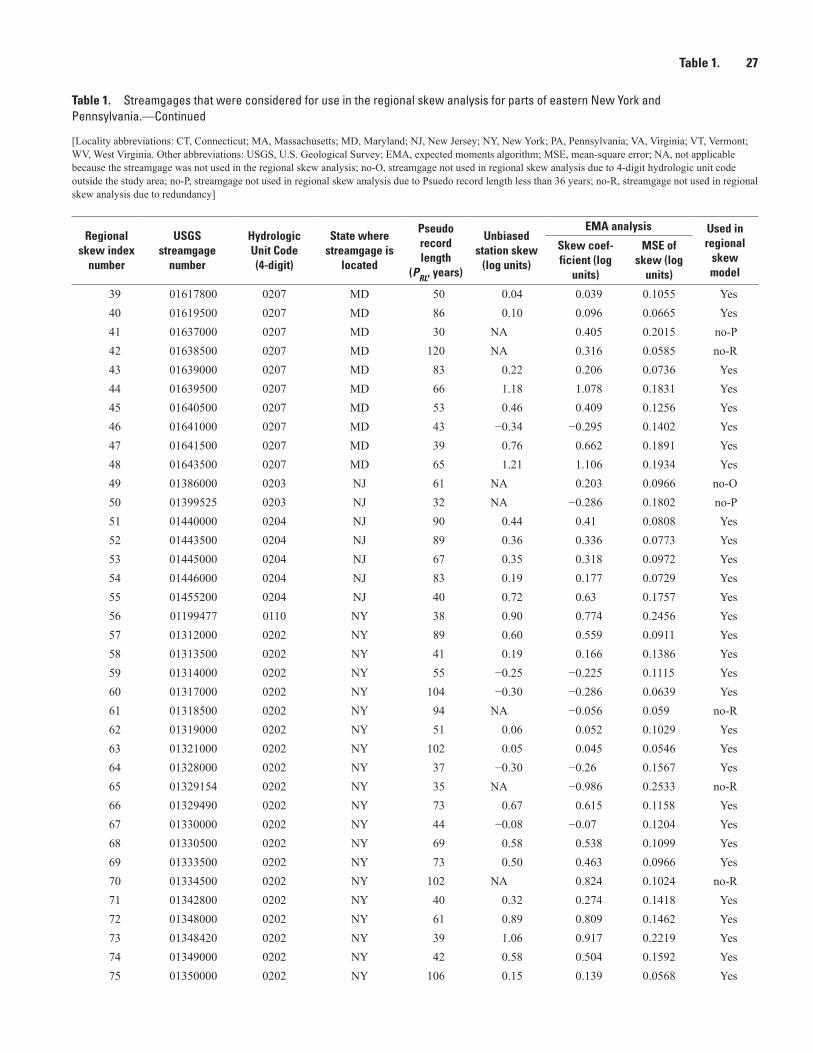
Table 1. 27
Table 1. Streamgages that were considered for use in the regional skew analysis for parts of eastern New York and Pennsylvania.—Continued
[Locality abbreviations: CT, Connecticut; MA, Massachusetts; MD, Maryland; NJ, New Jersey; NY, New York; PA, Pennsylvania; VA, Virginia; VT, Vermont; WV, West Virginia. Other abbreviations: USGS, U.S. Geological Survey; EMA, expected moments algorithm; MSE, mean-square error; NA, not applicable because the streamgage was not used in the regional skew analysis; no-O, streamgage not used in regional skew analysis due to 4-digit hydrologic unit code outside the study area; no-P, streamgage not used in regional skew analysis due to Psuedo record length less than 36 years; no-R, streamgage not used in regional skew analysis due to redundancy]
Regional skew index
number
USGS streamgage
number
Hydrologic Unit Code (4-digit)
State where streamgage is
located
Pseudo record length
(PRL, years)
Unbiased station skew
(log units)
EMA analysis Used in regional
skew model
Skew coef-ficient (log
units)
MSE of skew (log
units)
39 01617800 0207 MD 50 0.04 0.039 0.1055 Yes40 01619500 0207 MD 86 0.10 0.096 0.0665 Yes41 01637000 0207 MD 30 NA 0.405 0.2015 no-P42 01638500 0207 MD 120 NA 0.316 0.0585 no-R43 01639000 0207 MD 83 0.22 0.206 0.0736 Yes44 01639500 0207 MD 66 1.18 1.078 0.1831 Yes45 01640500 0207 MD 53 0.46 0.409 0.1256 Yes46 01641000 0207 MD 43 −0.34 −0.295 0.1402 Yes47 01641500 0207 MD 39 0.76 0.662 0.1891 Yes48 01643500 0207 MD 65 1.21 1.106 0.1934 Yes49 01386000 0203 NJ 61 NA 0.203 0.0966 no-O50 01399525 0203 NJ 32 NA −0.286 0.1802 no-P51 01440000 0204 NJ 90 0.44 0.41 0.0808 Yes52 01443500 0204 NJ 89 0.36 0.336 0.0773 Yes53 01445000 0204 NJ 67 0.35 0.318 0.0972 Yes54 01446000 0204 NJ 83 0.19 0.177 0.0729 Yes55 01455200 0204 NJ 40 0.72 0.63 0.1757 Yes56 01199477 0110 NY 38 0.90 0.774 0.2456 Yes57 01312000 0202 NY 89 0.60 0.559 0.0911 Yes58 01313500 0202 NY 41 0.19 0.166 0.1386 Yes59 01314000 0202 NY 55 −0.25 −0.225 0.1115 Yes60 01317000 0202 NY 104 −0.30 −0.286 0.0639 Yes61 01318500 0202 NY 94 NA −0.056 0.059 no-R62 01319000 0202 NY 51 0.06 0.052 0.1029 Yes63 01321000 0202 NY 102 0.05 0.045 0.0546 Yes64 01328000 0202 NY 37 −0.30 −0.26 0.1567 Yes65 01329154 0202 NY 35 NA −0.986 0.2533 no-R66 01329490 0202 NY 73 0.67 0.615 0.1158 Yes67 01330000 0202 NY 44 −0.08 −0.07 0.1204 Yes68 01330500 0202 NY 69 0.58 0.538 0.1099 Yes69 01333500 0202 NY 73 0.50 0.463 0.0966 Yes70 01334500 0202 NY 102 NA 0.824 0.1024 no-R71 01342800 0202 NY 40 0.32 0.274 0.1418 Yes72 01348000 0202 NY 61 0.89 0.809 0.1462 Yes73 01348420 0202 NY 39 1.06 0.917 0.2219 Yes74 01349000 0202 NY 42 0.58 0.504 0.1592 Yes75 01350000 0202 NY 106 0.15 0.139 0.0568 Yes

28 Methods for Estimating Regional Skewness of Annual Peak Flows in Parts of Eastern New York and Pennsylvania
Table 1. Streamgages that were considered for use in the regional skew analysis for parts of eastern New York and Pennsylvania.—Continued
[Locality abbreviations: CT, Connecticut; MA, Massachusetts; MD, Maryland; NJ, New Jersey; NY, New York; PA, Pennsylvania; VA, Virginia; VT, Vermont; WV, West Virginia. Other abbreviations: USGS, U.S. Geological Survey; EMA, expected moments algorithm; MSE, mean-square error; NA, not applicable because the streamgage was not used in the regional skew analysis; no-O, streamgage not used in regional skew analysis due to 4-digit hydrologic unit code outside the study area; no-P, streamgage not used in regional skew analysis due to Psuedo record length less than 36 years; no-R, streamgage not used in regional skew analysis due to redundancy]
Regional skew index
number
USGS streamgage
number
Hydrologic Unit Code (4-digit)
State where streamgage is
located
Pseudo record length
(PRL, years)
Unbiased station skew
(log units)
EMA analysis Used in regional
skew model
Skew coef-ficient (log
units)
MSE of skew (log
units)
76 01350120 0202 NY 38 0.63 0.541 0.1778 Yes77 01350140 0202 NY 39 −0.21 −0.186 0.1438 Yes78 01358500 0202 NY 59 1.47 1.336 0.2378 Yes79 01359528 0202 NY 55 0.40 0.362 0.113 Yes80 01359750 0202 NY 38 −0.19 −0.164 0.133 Yes81 01361000 0202 NY 70 0.63 0.577 0.1117 Yes82 01361500 0202 NY 107 −0.10 −0.091 0.0571 Yes83 01362100 0202 NY 56 0.41 0.367 0.1168 Yes84 01362197 0202 NY 33 NA −0.071 0.157 no-P85 01362200 0202 NY 69 NA 0.071 0.0784 no-R86 01362500 0202 NY 96 0.08 0.078 0.0585 Yes87 01365000 0202 NY 102 −0.29 −0.275 0.0631 Yes88 01365500 0202 NY 65 0.04 0.033 0.0828 Yes89 01368000 0202 NY 52 1.27 1.135 0.237 Yes90 01368500 0202 NY 51 1.01 0.901 0.1785 Yes91 01369000 0202 NY 40 0.56 0.488 0.1653 Yes92 01369500 0202 NY 42 0.28 0.242 0.1378 Yes93 01370000 0202 NY 54 NA 0.636 0.1453 no-R94 01371000 0202 NY 64 −0.22 −0.2 0.0841 Yes95 01371500 0202 NY 90 0.39 0.369 0.0785 Yes96 01372500 0202 NY 85 0.71 0.66 0.102 Yes97 01372800 0202 NY 44 0.04 0.031 0.1291 Yes98 01374250 0203 NY 39 NA 0.323 0.1664 no-O99 01387400 0203 NY 34 NA 0.756 0.2236 no-P
100 01387410 0203 NY 43 NA 0.095 0.1648 no-O101 01387450 0203 NY 53 NA 0.442 0.1282 no-O102 01413500 0204 NY 77 0.30 0.279 0.0838 Yes103 01414000 0204 NY 39 0.49 0.424 0.1632 Yes104 01414500 0204 NY 77 0.12 0.115 0.0745 Yes105 01415000 0204 NY 77 0.13 0.118 0.0747 Yes106 01418500 0204 NY 44 NA 0.103 0.1204 no-R107 01419500 0204 NY 39 NA 0.443 0.1633 no-R108 01420000 0204 NY 57 −0.07 −0.062 0.0948 Yes109 01420500 0204 NY 100 0.30 0.281 0.0669 Yes110 01421000 0204 NY 45 NA −0.039 0.1152 no-R111 01421900 0204 NY 57 0.08 0.071 0.0952 Yes112 01422500 0204 NY 55 −0.24 −0.217 0.1072 Yes
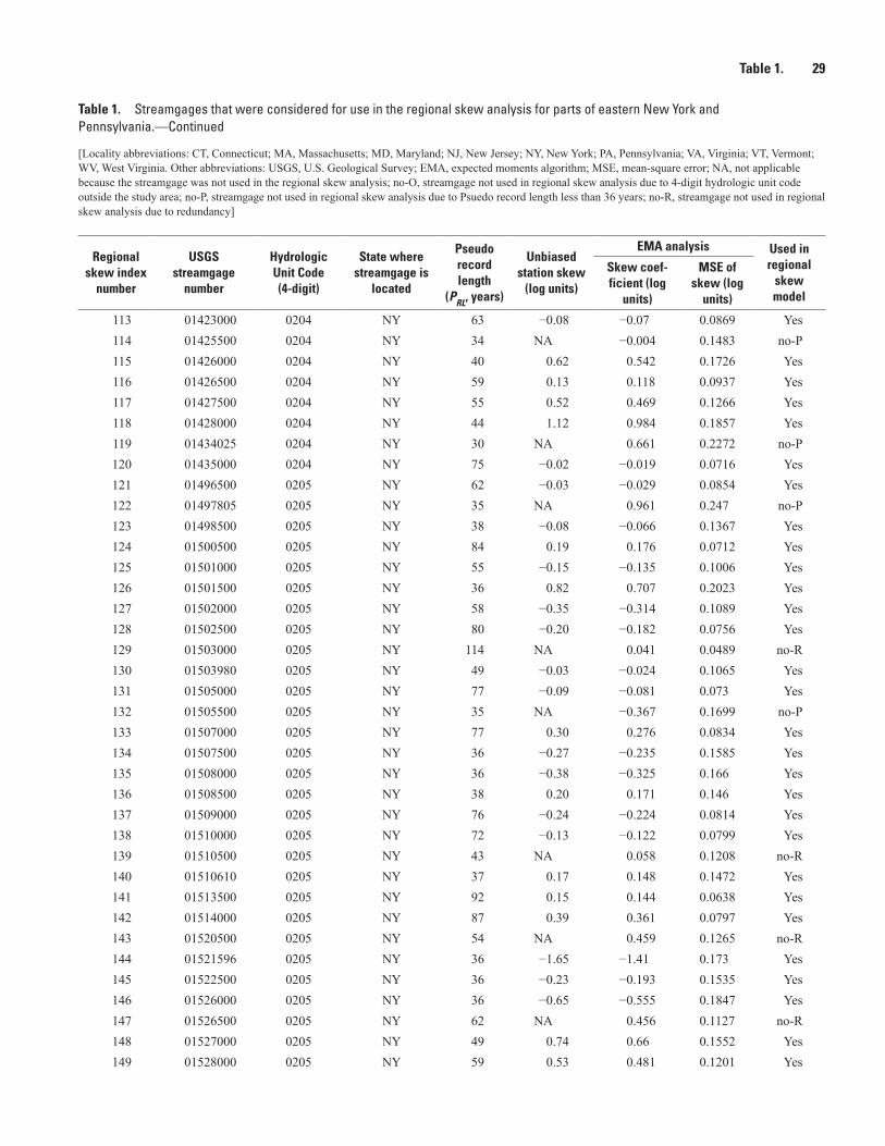
Table 1. 29
Table 1. Streamgages that were considered for use in the regional skew analysis for parts of eastern New York and Pennsylvania.—Continued
[Locality abbreviations: CT, Connecticut; MA, Massachusetts; MD, Maryland; NJ, New Jersey; NY, New York; PA, Pennsylvania; VA, Virginia; VT, Vermont; WV, West Virginia. Other abbreviations: USGS, U.S. Geological Survey; EMA, expected moments algorithm; MSE, mean-square error; NA, not applicable because the streamgage was not used in the regional skew analysis; no-O, streamgage not used in regional skew analysis due to 4-digit hydrologic unit code outside the study area; no-P, streamgage not used in regional skew analysis due to Psuedo record length less than 36 years; no-R, streamgage not used in regional skew analysis due to redundancy]
Regional skew index
number
USGS streamgage
number
Hydrologic Unit Code (4-digit)
State where streamgage is
located
Pseudo record length
(PRL, years)
Unbiased station skew
(log units)
EMA analysis Used in regional
skew model
Skew coef-ficient (log
units)
MSE of skew (log
units)
113 01423000 0204 NY 63 −0.08 −0.07 0.0869 Yes114 01425500 0204 NY 34 NA −0.004 0.1483 no-P115 01426000 0204 NY 40 0.62 0.542 0.1726 Yes116 01426500 0204 NY 59 0.13 0.118 0.0937 Yes117 01427500 0204 NY 55 0.52 0.469 0.1266 Yes118 01428000 0204 NY 44 1.12 0.984 0.1857 Yes119 01434025 0204 NY 30 NA 0.661 0.2272 no-P120 01435000 0204 NY 75 −0.02 −0.019 0.0716 Yes121 01496500 0205 NY 62 −0.03 −0.029 0.0854 Yes122 01497805 0205 NY 35 NA 0.961 0.247 no-P123 01498500 0205 NY 38 −0.08 −0.066 0.1367 Yes124 01500500 0205 NY 84 0.19 0.176 0.0712 Yes125 01501000 0205 NY 55 −0.15 −0.135 0.1006 Yes126 01501500 0205 NY 36 0.82 0.707 0.2023 Yes127 01502000 0205 NY 58 −0.35 −0.314 0.1089 Yes128 01502500 0205 NY 80 −0.20 −0.182 0.0756 Yes129 01503000 0205 NY 114 NA 0.041 0.0489 no-R130 01503980 0205 NY 49 −0.03 −0.024 0.1065 Yes131 01505000 0205 NY 77 −0.09 −0.081 0.073 Yes132 01505500 0205 NY 35 NA −0.367 0.1699 no-P133 01507000 0205 NY 77 0.30 0.276 0.0834 Yes134 01507500 0205 NY 36 −0.27 −0.235 0.1585 Yes135 01508000 0205 NY 36 −0.38 −0.325 0.166 Yes136 01508500 0205 NY 38 0.20 0.171 0.146 Yes137 01509000 0205 NY 76 −0.24 −0.224 0.0814 Yes138 01510000 0205 NY 72 −0.13 −0.122 0.0799 Yes139 01510500 0205 NY 43 NA 0.058 0.1208 no-R140 01510610 0205 NY 37 0.17 0.148 0.1472 Yes141 01513500 0205 NY 92 0.15 0.144 0.0638 Yes142 01514000 0205 NY 87 0.39 0.361 0.0797 Yes143 01520500 0205 NY 54 NA 0.459 0.1265 no-R144 01521596 0205 NY 36 −1.65 −1.41 0.173 Yes145 01522500 0205 NY 36 −0.23 −0.193 0.1535 Yes146 01526000 0205 NY 36 −0.65 −0.555 0.1847 Yes147 01526500 0205 NY 62 NA 0.456 0.1127 no-R148 01527000 0205 NY 49 0.74 0.66 0.1552 Yes149 01528000 0205 NY 59 0.53 0.481 0.1201 Yes

30 Methods for Estimating Regional Skewness of Annual Peak Flows in Parts of Eastern New York and Pennsylvania
Table 1. Streamgages that were considered for use in the regional skew analysis for parts of eastern New York and Pennsylvania.—Continued
[Locality abbreviations: CT, Connecticut; MA, Massachusetts; MD, Maryland; NJ, New Jersey; NY, New York; PA, Pennsylvania; VA, Virginia; VT, Vermont; WV, West Virginia. Other abbreviations: USGS, U.S. Geological Survey; EMA, expected moments algorithm; MSE, mean-square error; NA, not applicable because the streamgage was not used in the regional skew analysis; no-O, streamgage not used in regional skew analysis due to 4-digit hydrologic unit code outside the study area; no-P, streamgage not used in regional skew analysis due to Psuedo record length less than 36 years; no-R, streamgage not used in regional skew analysis due to redundancy]
Regional skew index
number
USGS streamgage
number
Hydrologic Unit Code (4-digit)
State where streamgage is
located
Pseudo record length
(PRL, years)
Unbiased station skew
(log units)
EMA analysis Used in regional
skew model
Skew coef-ficient (log
units)
MSE of skew (log
units)
150 01530301 0205 NY 36 −0.40 −0.343 0.1654 Yes151 01530500 0205 NY 54 −0.24 −0.212 0.1094 Yes152 01531000 0205 NY 78 0.16 0.144 0.0753 Yes153 0142400103 0204 NY 34 NA 0.344 0.1754 no-P154 01428750 0204 PA 39 1.13 0.983 0.2346 Yes155 01431000 0204 PA 43 0.30 0.266 0.1383 Yes156 01438300 0204 PA 52 0.02 0.015 0.1217 Yes157 01439500 0204 PA 105 1.02 0.964 0.1161 Yes158 01440400 0204 PA 56 −0.04 −0.037 0.0948 Yes159 01447500 0204 PA 70 0.70 0.645 0.117 Yes160 01448500 0204 PA 52 0.14 0.128 0.1074 Yes161 01449360 0204 PA 47 −1.50 −1.334 0.3029 Yes162 01450500 0204 PA 74 0.22 0.201 0.0821 Yes163 01451800 0204 PA 47 −0.12 −0.105 0.1205 Yes164 01453000 0204 PA 55 0.50 0.455 0.1254 Yes165 01459500 0204 PA 37 0.21 0.182 0.1504 Yes166 01470500 0204 PA 68 −0.05 −0.046 0.0798 Yes167 01470779 0204 PA 40 −0.14 −0.126 0.1353 Yes168 01472000 0204 PA 57 0.22 0.199 0.1025 Yes169 01472157 0204 PA 45 0.22 0.192 0.127 Yes170 01473000 0204 PA 99 −0.61 −0.571 0.0847 Yes171 01475850 0204 PA 37 0.29 0.25 0.1559 Yes172 01480300 0204 PA 54 −0.05 −0.041 0.0983 Yes173 01480675 0204 PA 47 −0.12 −0.103 0.116 Yes174 01516350 0205 PA 47 0.33 0.296 0.1255 Yes175 01516500 0205 PA 59 0.63 0.571 0.1275 Yes176 01532000 0205 PA 100 0.52 0.486 0.0786 Yes177 01534000 0205 PA 100 −0.33 −0.308 0.0683 Yes178 01538000 0205 PA 94 0.22 0.21 0.0668 Yes179 01539000 0205 PA 75 0.43 0.4 0.0928 Yes180 01541000 0205 PA 101 0.73 0.687 0.0911 Yes181 01541500 0205 PA 47 0.25 0.219 0.124 Yes182 01542810 0205 PA 50 0.77 0.69 0.1561 Yes183 01543000 0205 PA 100 0.38 0.354 0.0709 Yes184 01543500 0205 PA 75 NA 0.398 0.0927 no-R185 01544500 0205 PA 73 0.66 0.611 0.1103 Yes186 01545600 0205 PA 49 0.82 0.729 0.1623 Yes

Table 1. 31
Table 1. Streamgages that were considered for use in the regional skew analysis for parts of eastern New York and Pennsylvania.—Continued
[Locality abbreviations: CT, Connecticut; MA, Massachusetts; MD, Maryland; NJ, New Jersey; NY, New York; PA, Pennsylvania; VA, Virginia; VT, Vermont; WV, West Virginia. Other abbreviations: USGS, U.S. Geological Survey; EMA, expected moments algorithm; MSE, mean-square error; NA, not applicable because the streamgage was not used in the regional skew analysis; no-O, streamgage not used in regional skew analysis due to 4-digit hydrologic unit code outside the study area; no-P, streamgage not used in regional skew analysis due to Psuedo record length less than 36 years; no-R, streamgage not used in regional skew analysis due to redundancy]
Regional skew index
number
USGS streamgage
number
Hydrologic Unit Code (4-digit)
State where streamgage is
located
Pseudo record length
(PRL, years)
Unbiased station skew
(log units)
EMA analysis Used in regional
skew model
Skew coef-ficient (log
units)
MSE of skew (log
units)
187 01547700 0205 PA 58 0.71 0.64 0.1351 Yes188 01547950 0205 PA 46 0.28 0.25 0.1288 Yes189 01548005 0205 PA 60 −0.15 −0.138 0.0949 Yes190 01548500 0205 PA 95 0.53 0.503 0.083 Yes191 01549500 0205 PA 74 0.20 0.184 0.0806 Yes192 01550000 0205 PA 100 0.37 0.345 0.0703 Yes193 01552000 0205 PA 88 0.47 0.438 0.0841 Yes194 01552500 0205 PA 74 0.09 0.083 0.0755 Yes195 01553700 0205 PA 34 NA −0.076 0.1538 no-P196 01555000 0205 PA 84 0.45 0.418 0.0861 Yes197 01555500 0205 PA 84 1.14 1.061 0.1529 Yes198 01556000 0205 PA 98 0.41 0.391 0.0737 Yes199 01557500 0205 PA 72 0.08 0.074 0.0769 Yes200 01558000 0205 PA 75 1.10 1.018 0.1568 Yes201 01559000 0205 PA 112 NA 0.586 0.0782 no-R202 01560000 0205 PA 75 0.45 0.417 0.0948 Yes203 01562000 0205 PA 103 NA 0.244 0.0631 no-R204 01564500 0205 PA 83 0.32 0.298 0.0782 Yes205 01565000 0205 PA 60 0.53 0.486 0.1187 Yes206 01566000 0205 PA 79 0.17 0.157 0.074 Yes207 01567500 0205 PA 60 0.81 0.732 0.1397 Yes208 01568000 0205 PA 85 0.40 0.369 0.0825 Yes209 01570000 0205 PA 81 0.51 0.473 0.094 Yes210 01571500 0205 PA 69 1.03 0.946 0.1617 Yes211 01573000 0205 PA 95 1.32 1.241 0.1842 Yes212 01574000 0205 PA 85 1.66 1.553 0.2721 Yes213 01574500 0205 PA 36 0.90 0.769 0.2089 Yes214 01575000 0205 PA 43 1.02 0.891 0.1964 Yes215 01576500 0205 PA 85 0.31 0.29 0.0776 Yes216 01601000 0207 PA 47 NA 0.14 0.1185 no-R217 01603500 0207 PA 36 0.67 0.572 0.4171 Yes218 01613050 0207 PA 51 0.60 0.538 0.1403 Yes219 01613900 0207 VA 53 −0.05 −0.042 0.1001 Yes220 01615000 0207 VA 65 0.09 0.086 0.0849 Yes221 01634500 0207 VA 78 0.03 0.025 0.0691 Yes222 01638480 0207 VA 43 −0.35 −0.304 0.1409 Yes223 01142500 0108 VT 152 NA 0.568 0.0517 no-O
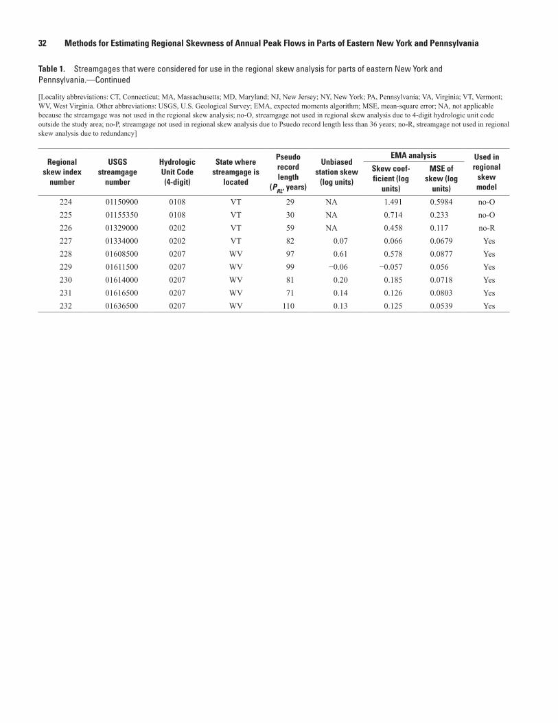
32 Methods for Estimating Regional Skewness of Annual Peak Flows in Parts of Eastern New York and Pennsylvania
Table 1. Streamgages that were considered for use in the regional skew analysis for parts of eastern New York and Pennsylvania.—Continued
[Locality abbreviations: CT, Connecticut; MA, Massachusetts; MD, Maryland; NJ, New Jersey; NY, New York; PA, Pennsylvania; VA, Virginia; VT, Vermont; WV, West Virginia. Other abbreviations: USGS, U.S. Geological Survey; EMA, expected moments algorithm; MSE, mean-square error; NA, not applicable because the streamgage was not used in the regional skew analysis; no-O, streamgage not used in regional skew analysis due to 4-digit hydrologic unit code outside the study area; no-P, streamgage not used in regional skew analysis due to Psuedo record length less than 36 years; no-R, streamgage not used in regional skew analysis due to redundancy]
Regional skew index
number
USGS streamgage
number
Hydrologic Unit Code (4-digit)
State where streamgage is
located
Pseudo record length
(PRL, years)
Unbiased station skew
(log units)
EMA analysis Used in regional
skew model
Skew coef-ficient (log
units)
MSE of skew (log
units)
224 01150900 0108 VT 29 NA 1.491 0.5984 no-O225 01155350 0108 VT 30 NA 0.714 0.233 no-O226 01329000 0202 VT 59 NA 0.458 0.117 no-R227 01334000 0202 VT 82 0.07 0.066 0.0679 Yes228 01608500 0207 WV 97 0.61 0.578 0.0877 Yes229 01611500 0207 WV 99 −0.06 −0.057 0.056 Yes230 01614000 0207 WV 81 0.20 0.185 0.0718 Yes231 01616500 0207 WV 71 0.14 0.126 0.0803 Yes232 01636500 0207 WV 110 0.13 0.125 0.0539 Yes

Appendix 1. 33
Appendix 1. Assessment of a Regional Skew Model for Parts of Eastern New York and Pennsylvania by Using Monte Carlo Simulations
This appendix provides a graphical assessment of the Bayesian weighted least squares/Bayesian generalized least squares (B–WLS/B–GLS) model of regional skew for parts of eastern New York and Pennsylvania that is described in this report. Observed, unbiased station skews are depicted in figure 1.1 along with contour lines and shading to provide a sense of geographic patterns in the skews.
Monte Carlo simulations were used to determine whether geographic patterns observed in the station skews are evidence of significant model misspecification or an artifact of random-sampling variability that is possibly confounded by the covari-ance structure of the errors. The Monte Carlo simulations were generated from a multivariate normal distribution with a mean equal to the constant from the regional skew model and
a covariance matrix identical to the covariance matrix used in the regional skew model. The constant model of skew in the study area is:
– / – 0ˆ .32B WLS B GLS = + , (1.1)
where ε represents the total error, and
� �~ ,N Var0 � �� �, (1.2)
where N signifies a normal distribution of the total
error in the constant regional skew model determined in the B–GLS analysis.
res20-0073_fig01.01
Unbiased skew
Lake Erie
Lake Ontario
ATLANTIC OCEAN
VIRGINIA
PENNSYLVANIA
NEW YORK
CONNECTICUT
DELAWARE
NEWJERSEY
NH
WEST
VERMONT
VIRGINIA
CANADA
UNITED STATES
Base from U.S. Geological Survey digital data,various dates and scalesNorth American Datum of 1983
0 100 200 MILES
0 100 200 KILOMETERS
42°
44°
43°
39°
41°
40°
80° 78° 76° 74° 72°
Unbiased skew
Location of streamgage
EXPLANATION
>1.01.0 to 0.760.75 to 0.510.50 to 0.260.25 to 0.110.10 to –0.10–0.11 to –0.25–0.26 to –0.50–0.51 to –0.75–0.76 to –1.0<–1.0
MARYLAND
MASSACHUSETTS
Figure 1.1. Contour map of unbiased station skews for the 183 streamgages that were used in the regional skew analysis for parts of eastern New York and Pennsylvania.

34 Methods for Estimating Regional Skewness of Annual Peak Flows in Parts of Eastern New York and Pennsylvania
As described in equation 1.2, the Var �� � can be described as
� � � �2 2– , , ˆTB GLS B GLS B GLSδ δεε σ σ� �� � � � �� � Λ I Σ γ , (1.3)
where εT is the transformation of ε, � �2
– ,B GLS B GLSδσ �Λ is the (n × n) B–GLS covariance matrix,
�� ,B GLS�2 is the B–GLS variance of the underlying
model error δ, I is an (n × n) identity matrix, and � �ˆΣ γ is the full (n × n) covariance matrix of the
sampling errors for each streamgage (n).
The covariance matrix of the sampling errors is made up of the sampling variances of the unbiased station skew ( � �ˆiVar γ ) and the covariances of the skewness estimators ( ˆiγ ). The off-diagonal values of � �ˆΣ γ are determined by the cross correlation of concurrent gaged annual peak flows and the cf factor (see equation 3 in Martins and Stedinger, 2002). The model error variance ��
2 for the constant model is
0.10 (table 3) and was used in the Monte Carlo simulations. The covariance matrix � �ˆΣ γ used in the Monte Carlo simula-tions is the same as that used in the B–WLS/B–GLS regres-sion analysis (see eqs. 18 and 19 in the report).
The results of the Monte Carlo simulations are depicted graphically in 20 realizations (fig. 1.2) of the expected patterns in the station skew if the station skews are normally distrib-uted with a mean equal to 0.32 and a covariance matrix given by equation 1.3. The Monte Carlo simulations reveal no struc-ture in the pattern of the station skews that is consistent with the observed pattern of the station skews in the constant model (fig. 1.1). Therefore, it seems reasonably safe to conclude that, despite the geographic patterns observed in the station skews, there is little evidence of a lack of fit.
Reference Cited
Martins, E.S., and Stedinger, J.R., 2002, Cross correlations among estimators of shape: Water Resources Research, v. 38, no. 11, p. 34-1 to 34-7. [Also available at https://doi.org/ 10.1029/ 2002WR001589.]

Appendix 1. 35
ATLANTIC OCEAN ATLANTIC OCEAN
ATLANTIC OCEAN ATLANTIC OCEAN
ATLANTIC OCEAN
Lake Ontario
Lake Erie
Lake Ontario
Lake Erie
Lake Ontario
Lake Erie
Lake Ontario
Lake Erie
Lake Ontario
Lake Erie
VA
PA
NY
CT
MA
DE
NJ
NH
WV
VTCANADA
UNITED STATES
VA
PA
NY
CT
MA
DE
NJ
NH
WV
VTCANADA
UNITED STATES
VA
PA
NY
CT
MA
DE
NJ
NH
WV
VTCANADA
UNITED STATES
VA
PA
NY
CT
MA
DE
NJ
NH
WV
VTCANADA
UNITED STATES
VA
PA
NY
CT
MA
DE
NJ
NH
WV
VTCANADA
UNITED STATES
Base from U.S. Geological Surveydigital data, various dates and scalesNorth American Datum of 1983
0 100 200 MILES
0 100 200 KILOMETERS
42°
44°
43°
39°
41°
40°
80° 78° 76° 74° 72° 80° 78° 76° 74° 72°
42°
44°
43°
39°
41°
40°
42°
44°
43°
39°
41°
40°
Unbiased skew
Location of streamgage
EXPLANATION
>1.01.0 to 0.760.75 to 0.510.50 to 0.260.25 to 0.110.10 to –0.10–0.11 to –0.25–0.26 to –0.50–0.51 to –0.75–0.76 to –1.0<–1.0
MD
A
MD
B
MD
C
MD
D
MD
E
Figure 1.2. Contour maps showing the results of 20 Monte Carlo simulations (A–T) of unbiased station skew at 183 streamgages that were used in the regional skew analysis for parts of eastern New York and Pennsylvania. Simulations are normally distributed to the constant skew model and covariance matrix.

36 Methods for Estimating Regional Skewness of Annual Peak Flows in Parts of Eastern New York and Pennsylvania
ATLANTIC OCEAN ATLANTIC OCEAN
ATLANTIC OCEAN ATLANTIC OCEAN
ATLANTIC OCEAN
Lake Ontario
Lake Erie
Lake Ontario
Lake Erie
Lake Ontario
Lake Erie
Lake Ontario
Lake Erie
Lake Ontario
Lake Erie
VA
PA
NY
CT
MA
DE
NJ
NH
WV
VTCANADA
UNITED STATES
VA
PA
NY
CT
MA
DE
NJ
NH
WV
VTCANADA
UNITED STATES
VA
PA
NY
CT
MA
DE
NJ
NH
WV
VTCANADA
UNITED STATES
VA
PA
NY
CT
MA
DE
NJ
NH
WV
VTCANADA
UNITED STATES
VA
PA
NY
CT
MA
DE
NJ
NH
WV
VTCANADA
UNITED STATES
Base from U.S. Geological Surveydigital data, various dates and scalesNorth American Datum of 1983
0 100 200 MILES
0 100 200 KILOMETERS
42°
44°
43°
39°
41°
40°
80° 78° 76° 74° 72° 80° 78° 76° 74° 72°
42°
44°
43°
39°
41°
40°
42°
44°
43°
39°
41°
40°
Unbiased skew
Location of streamgage
EXPLANATION
>1.01.0 to 0.760.75 to 0.510.50 to 0.260.25 to 0.110.10 to –0.10–0.11 to –0.25–0.26 to –0.50–0.51 to –0.75–0.76 to –1.0<–1.0
MD
F
MD
G
MD
H
MD
I
MD
J
Figure 1.2.—Continued

Appendix 1. 37
ATLANTIC OCEAN ATLANTIC OCEAN
ATLANTIC OCEAN ATLANTIC OCEAN
ATLANTIC OCEAN
Lake Ontario
Lake Erie
Lake Ontario
Lake Erie
Lake Ontario
Lake Erie
Lake Ontario
Lake Erie
Lake Ontario
Lake Erie
VA
PA
NY
CT
MA
DE
NJ
NH
WV
VTCANADA
UNITED STATES
VA
PA
NY
CT
MA
DE
NJ
NH
WV
VTCANADA
UNITED STATES
VA
PA
NY
CT
MA
DE
NJ
NH
WV
VTCANADA
UNITED STATES
VA
PA
NY
CT
MA
DE
NJ
NH
WV
VTCANADA
UNITED STATES
VA
PA
NY
CT
MA
DE
NJ
NH
WV
VTCANADA
UNITED STATES
Base from U.S. Geological Surveydigital data, various dates and scalesNorth American Datum of 1983
0 100 200 MILES
0 100 200 KILOMETERS
42°
44°
43°
39°
41°
40°
80° 78° 76° 74° 72° 80° 78° 76° 74° 72°
42°
44°
43°
39°
41°
40°
42°
44°
43°
39°
41°
40°
Unbiased skew
Location of streamgage
EXPLANATION
>1.01.0 to 0.760.75 to 0.510.50 to 0.260.25 to 0.110.10 to –0.10–0.11 to –0.25–0.26 to –0.50–0.51 to –0.75–0.76 to –1.0<–1.0
MD
K
MD
L
MD
M
MD
N
MD
O
Figure 1.2.—Continued
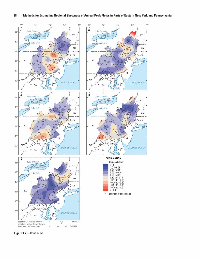
38 Methods for Estimating Regional Skewness of Annual Peak Flows in Parts of Eastern New York and Pennsylvania
ATLANTIC OCEAN ATLANTIC OCEAN
ATLANTIC OCEAN ATLANTIC OCEAN
ATLANTIC OCEAN
Lake Ontario
Lake Erie
Lake Ontario
Lake Erie
Lake Ontario
Lake Erie
Lake Ontario
Lake Erie
Lake Ontario
Lake Erie
VA
PA
NY
CT
MA
DE
NJ
NH
WV
VTCANADA
UNITED STATES
VA
PA
NY
CT
MA
DE
NJ
NH
WV
VTCANADA
UNITED STATES
UNITED STATES
VA
PA
NY
CT
MA
DE
NJ
NH
WV
VTCANADA
UNITED STATES
VA
PA
NY
CT
MA
DE
NJ
NH
WV
VTCANADA
VA
PA
NY
CT
MA
DE
NJ
NH
WV
VTCANADA
UNITED STATES
Base from U.S. Geological Surveydigital data, various dates and scalesNorth American Datum of 1983
0 100 200 MILES
0 100 200 KILOMETERS
42°
44°
43°
39°
41°
40°
80° 78° 76° 74° 72° 80° 78° 76° 74° 72°
42°
44°
43°
39°
41°
40°
42°
44°
43°
39°
41°
40°
Unbiased skew
Location of streamgage
EXPLANATION
>1.01.0 to 0.760.75 to 0.510.50 to 0.260.25 to 0.110.10 to –0.10–0.11 to –0.25–0.26 to –0.50–0.51 to –0.75–0.76 to –1.0<–1.0
MD
P
MD
Q
MD
R
MD
S
MD
T
Figure 1.2.—Continued


Veilleux and Wagner—
Methods for Estim
ating Regional Skewness of A
nnual Peak Flows in Parts of Eastern N
ew York and Pennsylvania—
SIR 2021–5015
ISSN 2328-0328 (online)https://doi.org/ 10.3133/ sir20215015