Embed Size (px)
Citation preview
University of West Bohemia Department of Computer Science and Engineering Univerzitní 8 CZ 306 14 Plzen Czech Republic
Methods for dynamic mesh size reduction State of the Art and concept of doctoral thesis Libor Váša Technical Report No. DCSE/TR-2006-07 October, 2006 Distribution: public
Libor Váša - Methods for dynamic mesh size reduction - State of the Art
- 2 -
Abstract This work focuses on processing of dynamic meshes, i.e. series of triangular meshes of
equal connectivity which represent an evolution of a model in time. The main goal is to reduce the storage and transmission cost. The work covers the state of the art in the fields of compression and simplification of triangular meshes.
By compression we mean methods of encoding the mesh without altering its connectivity. Usually some sort of vertex position prediction is used, combined with delta coding of residuals. PCA (Principal Component Analysis) based compression methods are also mentioned.
The simplification methods on the other hand reduce the storage cost of a dynamic mesh by changing its connectivity. There are only a few methods that are directly targeted on dynamic mesh simplification, and therefore we also discuss methods for static mesh simplification.
In the last section of the state of the art we present methods for comparing dynamic meshes that can be used to evaluate the processing methods. We present the basic MSE based PSNR metric, we point out is disadvantages, and present our solution to this problem based on Hausdorff distance.
In the last chapter we discuss the possible directions of future research in the fields of compression and simplification methods. We sketch possible ways of extension of the static mesh simplification methods to the dynamic case, and we also discuss some minor concrete ideas for improvement in the field covered by the state of the art.
keywords: animation, compression, triangle mesh, dynamic mesh, simplification, reduction
Abstrakt Tato práce se zabývá zpracováním dynamických sítí. Dynamickou sítí rozumíme sérii
trojúhelníkových sítí které mají stejnou konektivitu, jež představují časový vývoj objektu. Naším hlavním cílem je snížení velikosti datové reprezentace dynamické sítě. Tato práce pokrývá současný stav výzkumu v oblastech komprese a simplifikace dynamických sítí.
Jako kompresi označujeme takové metody uložení dynamické sítě, které nemění její konektivitu. Obvyklým přístupem je vytvoření nějakého prediktoru polohy vektoru, jehož predikce je pak korigována pomocí delta-coding strategie. Práce rovněž zmiňuje metody založené na PCA (Principal Component Analysis).
Narozdíl od kompresí, simplifikace obecně dosahují snížení velikosti dat obecnou změnou konektivity. V literatuře je popsáno jen málo metod pro simplifikaci dynamických sítí, a proto se práce zabývá rovněž metodami pro kompresi statických sítí a možnostmi jejich rozšíření.
V poslední části zprávy se zabýváme metodami porovnávání dynamických sítí, které je možno použít pro zhodnocení efektivity kompresních a simplifikačních metod. Práce se zabývá přístupem založeným na průměrné odchylce, zmiňuje nevýhody této metody a odvozuje metriku založenou na Hausdorffově vzdálenosti.
V závěrečné kapitole se zabýváme možnostmi dalšího výzkumu v oblastech komprese a simplifikace dynamických sítí. Nastiňujeme možná rozšíření metod pro simplifikaci statických sítí pro dynamický případ, a rovněž zmiňujeme několik konkrétních menších vylepšení metod popsaných v teoretické části.
klíčová slova: animace, komprese, trojúhelníková síť, dynamická síť, simplifikace,
zjednodušení

Libor Váša - Methods for dynamic mesh size reduction - State of the Art
- 3 -
Acknowledgements The author would like to thank Aljosha Smolic and Yucel Yemez for providing valuable
resources, and to his colleagues, Martin Janda, Slavo Petrík and Petr Vaněček for numerous consultations and comments.
This work has been supported by the project 3DTV PF6-2003-IST-2, Network of Excellence, No: 511568 and by the project Centre of Computer Graphics – National Network of Fundamental Research Centers, MSMT Czech Rep., No: LC 06008
Libor Váša - Methods for dynamic mesh size reduction - State of the Art
- 4 -
Table of contents Abstract .........................................................................................................................................................- 2 - Abstrakt .........................................................................................................................................................- 2 - Acknowledgements .......................................................................................................................................- 3 - Table of contents ...........................................................................................................................................- 4 - 1 Introduction ..........................................................................................................................................- 5 -
1.1 Problem definition.......................................................................................................................- 5 - 1.2 Organization................................................................................................................................- 7 -
2 Compression .........................................................................................................................................- 8 - 2.1 Geometry compression of dynamic meshes ................................................................................- 8 -
2.1.1 Predictor approaches ..............................................................................................................- 8 - 2.1.2 Notation..................................................................................................................................- 8 - 2.1.3 Pure temporal predictors.........................................................................................................- 9 - 2.1.4 Pure spatial predictors ............................................................................................................- 9 - 2.1.5 Space-time predictors ...........................................................................................................- 10 - 2.1.6 Muller approach ...................................................................................................................- 11 - 2.1.7 Wavelet based compression..................................................................................................- 12 - 2.1.8 PCA based compression .......................................................................................................- 13 - 2.1.9 PCA LPC coding ..................................................................................................................- 14 - 2.1.10 Clustering based PCA encoding ......................................................................................- 15 -
2.2 Triangular connectivity compression ........................................................................................- 16 - 2.2.1 Topological Surgery .............................................................................................................- 16 - 2.2.2 EdgeBreaker/cut-border machine .........................................................................................- 18 - 2.2.3 Delphi geometry based connectivity encoding.....................................................................- 20 -
2.3 Tetrahedral connectivity compression.......................................................................................- 20 - 2.3.1 Grow&Fold ..........................................................................................................................- 20 - 2.3.2 Cut-border ............................................................................................................................- 21 -
3 Simplification .....................................................................................................................................- 23 - 3.1 Triangular simplification...........................................................................................................- 23 -
3.1.1 Schroeder decimation ...........................................................................................................- 23 - 3.1.2 Attene – SwingWrapper .......................................................................................................- 25 - 3.1.3 Geometry images..................................................................................................................- 27 - 3.1.4 Edge collapse........................................................................................................................- 28 - 3.1.5 Quadric based .......................................................................................................................- 30 - 3.1.6 Locally volume preserving edge collapse.............................................................................- 31 -
3.2 Dynamic mesh simplification....................................................................................................- 33 - 3.2.1 Geometry video ....................................................................................................................- 33 - 3.2.2 Quadric based simplification in higher dimension ...............................................................- 33 - 3.2.3 TetFusion..............................................................................................................................- 35 - 3.2.4 Average quadric based simplification ..................................................................................- 37 - 3.2.5 Quadric based multiresolution mesh ....................................................................................- 37 -
4 Evaluation tools ..................................................................................................................................- 40 - 4.1.1 PSNR....................................................................................................................................- 40 - 4.1.2 Mesh, METRO .....................................................................................................................- 40 -
5 Published original contributions .........................................................................................................- 42 - 5.1 4D tetrahedral mesh representation ...........................................................................................- 42 -
5.1.1 4D metric..............................................................................................................................- 43 - 6 Proposal of future research .................................................................................................................- 46 -
6.1 Dynamic mesh compression......................................................................................................- 46 - 6.2 Dynamic mesh simplification....................................................................................................- 49 -
6.2.1 Frame by frame simplification .............................................................................................- 49 - 6.2.2 Spatio-temporal simplification .............................................................................................- 49 - 6.2.3 Single connectivity simplification ........................................................................................- 50 - 6.2.4 Multiresolution approach......................................................................................................- 51 -
References ...................................................................................................................................................- 53 - Publications .................................................................................................................................................- 55 - Appendix A – Project assignments, other activities ....................................................................................- 56 -
Stays abroad............................................................................................................................................- 56 - Teaching activities:.................................................................................................................................- 56 -
Libor Váša - Methods for dynamic mesh size reduction - State of the Art
- 5 -
1 Introduction Computer graphics is one of the most constantly developing areas of computer science.
While the growth of processing power of common PCs seems to slow down in the last years, computer graphics related hardware is developing still very rapidly, and computer graphics as a supporting science is reaching to problems that seemed impossible just a few years ago.
In the past, computer graphics gave answers to some non-trivial questions related to displaying and processing virtual models. The key issue for most of the computer graphics-related problems is the problem of computational complexity. In other words, the results in computer graphics must not only be correct, but they also need to be delivered in a reasonable time.
The problems of computer graphics span from the data acquisition (polygonization and tessellation algorithms) through various processing techniques (simplification, stripification etc.) up to the displaying itself (shading, rendering). Most of the algorithms in each of the areas are designed to provide the best possible quality/performance ratio, so that current limited hardware can process as complex (and therefore realistic) scenes as possible. However, the recent development of accelerating hardware is not making the old problems and their solutions obsolete, it merely allows new problems to be solved.
A typical case where recent hardware progresses have allowed broadening of horizons of
solvable problems is the current possibility of studying time-variant cases of problems that were so far only studied in their static forms. Current hardware allows real-time acquisition of data on one hand, while emerging display devices allow delivering full 3D impression of a dynamic virtual scene to the user. The applications span from scientific problems, such as dynamic volume data processing, up to pure entertainment, such as 3D television.
While some of the current algorithms used for processing of static scenes can be used directly for the dynamic case, a large group of existing solutions cannot be used in dynamic case at all, or only at high processing cost. This gives us a wide new area for research, where it seems to be useful to take a look at the old problems from a slightly different point of view. The sophisticated algorithms for static problems give us good platform for such research, but for many problems a completely new approaches are likely to rise.
Problem of storage requirements is closely related to the general performance criterion.
Large and complex meshes allow high precision, but also require high processing power. The problem of transmission of models is also of increasing importance, as today’s network connections are still limited in their bandwidth.
The problem of reduction of storage requirements has been addressed by several approaches for the case of static meshes, while in recent years a more complex dynamic case is also being considered, which is also the main topic of this work. We will show the main current approaches used for static case, we will present some first results for the dynamic case, and we will propose directions for further research in this area.
1.1 Problem definition In this work we will focus our effort on a special case of the problem described in the
introduction. We will be considering the case of constant connectivity dynamic triangular meshes, and we will be investigating possibilities of compression and simplification of such meshes.
A triangular mesh is a spatial dataset, which represents a surface of an object. It consists of geometry and topology. Geometry information is usually represented by a set of three component vectors, each vector representing one point in a 3D space. Topology information is
Libor Váša - Methods for dynamic mesh size reduction - State of the Art
- 6 -
usually represented by a set of index triplets, where each triplet represents indices of three vertices of the mesh topology, which form a triangle.
For some algorithms it is crucial to differentiate between so-called manifold and non-manifold meshes. Manifold meshes are defined by several additional conditions for the mesh topology. These are:
- each edge is shared by at most two triangles - neighborhood of each vertex is topologically equivalent with a disc or a border.
Of importance is also a so-called simple mesh. A simple mesh is a genus 0 manifold mesh,
i.e. a closed single component mesh with no holes. Such mesh can be mapped onto a sphere, and it is often used as the simplest basic case on which algorithms are demonstrated.
A dynamic mesh is an ordered set of static meshes, where subsequent meshes represent the
development of the mesh over time. In other words, dynamic mesh represents an animation of a 3D surface. In the most usual case, we have one mesh for each frame that is captured, and the time span between the meshes is 1/frame rate. However it is possible to also consider meshes where each frame carries explicit information about the time when it occurs, and where the inter-frame times are not equal.
One important assumption for this work is the one of constant connectivity of the input. We assume that the topology information does not change between subsequent frames. This implies that we have the explicit information about the correspondence of vertices, edges and triangles of subsequent frames. It also implies that the number of vertices and triangles does not change throughout the animation. We can also see the situation as a simple movement of vertex position over time, where each vertex moves between two subsequent frames from it’s position in the first frame to it’s position in the second frame.
Please note that we are only making this assumption about the input data, while the output data may be of varying connectivity. Also note that we assume that no other information about the viewer is given, i.e. we don’t know anything about the relative position of the camera and the object.
There are several approaches to reduction of storage requirements. The most important aspect of reduction is the purpose of the final data. Approaches used for reduction of scientific data follow different criteria than algorithms targeted at human perception. In the first case, the main and only property of reduction algorithm is the reduction/error ratio, where the error is exactly determined by the nature of the data. On the other hand, when the target is a human observer, then the main quality of a reduction algorithm is the reduction/disturbance ratio. In this case, the algorithms may use some special properties of human perception to achieve better reduction rates with equal perceived distortion. In this work we will not be considering reduction for scientific purposes, our only criterion is the visual disturbance.
Our aim is to find and compare algorithms that take a dynamic mesh of constant
connectivity as an input, and create a different dynamic mesh, which is visually equivalent to the original one, while its storage requirements are reduced.
The approaches to storage requirements reduction can be divided into two main categories,
compressions and simplifications. Compressions are methods that encode the input data in a way that reduces storage requirements, while simplifications modify the input data in order to remove parts that are not necessary for the observer.
Libor Váša - Methods for dynamic mesh size reduction - State of the Art
- 7 -
Compressions can be applied to geometry, topology or both, and we differentiate between lossy and lossless compressions. Simplifications always involve alterations to both geometry and topology.
1.2 Organization The rest of this study is divided into two main parts. In the first part, we describe existing
approaches to the problem outlined above, and in the second we propose some directions where the existing approaches can be extended to either cover the dynamic case, or to cover it better.
In the state of the art part we will briefly outline approaches used for compression (chapter 2), simplification (chapter 3) and comparison (chapter 4) of static triangular meshes, as well as some methods that are designed for or can be used for the dynamic case. In chapter 5 we will discuss some of our own additions to the state of the art that have been already published. Chapter 6 concludes this material with analysis of the weaknesses of the methods described in the state of the art chapters, and proposal of future research focused on overcoming the identified drawbacks.
Libor Váša - Methods for dynamic mesh size reduction - State of the Art
- 8 -
2 Compression Compression in our context means a way of encoding the input dynamic mesh, which does
not change the topology of the mesh. There are two main approaches to the problem, each targeted on different redundancy present in the data. In the first case, algorithms try to exploit redundancy in the geometry information. The other approach is to exploit the redundancy in the connectivity encoding, especially when the geometry is already known (i.e. already decoded).
For the case of geometry compression, algorithms processing dynamic meshes were already proposed. The usual scheme is to encode the first frame as full information, and then to encode only the differences in the positions of the vertices in the next frame. The algorithm usually contains a predictor that estimates the position of the vertex from the positions of the already encoded/decoded vertices, and then encodes the difference between the real position of the vertex and the predicted one. Sophisticated prediction techniques were used, some of which will be mentioned in the following text.
For the case of connectivity compression, only the static case has been investigated so far. This however does not cause any problem, as our task only involves one constant connectivity. The algorithms proposed in the literature usually involve some sophisticated way of encoding a progress of some open border, which traverses through the mesh. The key is usually in encoding the most common cases with the shortest possible bit sequence. The proposed algorithms work with both triangle and tetrahedral meshes, and we will later show how static tetrahedral mesh can be used to represent a dynamic mesh.
There are also hybrid compression techniques, which combine topology and geometry compression into one algorithm. Such techniques can be elegantly extended to cover the case of dynamic meshes.
2.1 Geometry compression of dynamic meshes
2.1.1 Predictor approaches There are several predictors used for dynamic mesh compression. The main quality of a
predictor is its accuracy, because the arithmetic coding block that follows the estimator works best when the average residual vector is as short as possible.
Some of the predictors take as input only vertices from the frame that is currently being encoded, which may lead to need of specific ordering of the vertices, denoted as „connectivity based encoding“, which means that a vertex can be encoded only when at least two of it’s neighbors are already encoded. Fortunately, such ordering comes naturally with some of the connectivity encoding schemes that will be described in more detail later. Such predictors only use spatial coherence of the input data.
On the other hand, there are some very simple predictors that only use the vertex positions from previous frame, thus exploiting only temporal coherence of the input. However, the most sophisticated prediction schemes exploit both temporal and spatial coherence of the input data.
2.1.2 Notation Let’s denote the vertex positions as follows: p(v,f) – position of a vertex v in time frame f pred(v,f) – prediction of the position of the vertex v in time frame f
Libor Váša - Methods for dynamic mesh size reduction - State of the Art
- 9 -
2.1.3 Pure temporal predictors The simplest way to predict a position of a vertex is to set the prediction into the vertex
position from the previous frame:
( ) ( )1v, f- p v, fpred stat = We can also approximate the vertex motion by linear motion (constant velocity), and set
the prediction as follows:
( ) ( ) ( ) ( )( )211 v, f- - pv,f-p v,f- p v,fpredlin += Constant acceleration predictor is then a simple extension of the constant velocity
predictor, only this time requiring three previous time frames and using quadratic extrapolation
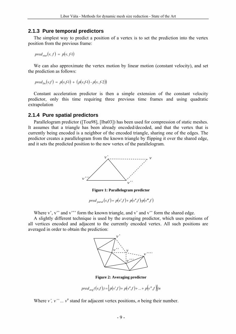
2.1.4 Pure spatial predictors Parallelogram predictor ([Tou98], [Iba03]) has been used for compression of static meshes.
It assumes that a triangle has been already encoded/decoded, and that the vertex that is currently being encoded is a neighbor of the encoded triangle, sharing one of the edges. The predictor creates a parallelogram from the known triangle by flipping it over the shared edge, and it sets the predicted position to the new vertex of the parallelogram.
Figure 1: Parallelogram predictor
( ) ( ) ( ) ( ),fv-p,fvp,fvpv,fpred paral ′′′′′+′=
Where v’, v’’ and v’’’ form the known triangle, and v’ and v’’ form the shared edge. A slightly different technique is used by the averaging predictor, which uses positions of
all vertices encoded and adjacent to the currently encoded vertex. All such positions are averaged in order to obtain the prediction:
Figure 2: Averaging predictor
( ) ( ) ( ) ( )[ ]/n,fvp...,fvp,fvp)v,f(pred n
avg ++′′+′= Where v’, v’’ ... vn stand for adjacent vertex positions, n being their number.
vv’
v’’v’’’
v
v’
v’’
v’’’v’’’’
Libor Váša - Methods for dynamic mesh size reduction - State of the Art
- 10 -
2.1.5 Space-time predictors Yang et al. [Yan02] have proposed a time-space predictor based on the averaging space-
only predictor, denoted as motion vector averaging predictor. The idea is that a vertex is expected to move in a way similar to its neighbors. This assumption leads to following predictor formula:
( ) ( ) ( ) ( )11 −+−= v,fpv,f-predv,f pred v,fpred avgavgmvavg
In [Iba03] Ibarria and Rossignac have proposed two space-time predictors, the ELP
(Extended Lorenzo Predictor) and the Replica predictor as a part of their Dynapack algorithm. The ELP predictor is a perfect predictor for meshes that undergo a translational only
movement, i.e. for such meshes it estimates the new position of each vertex exactly. The formulation of the predictor can be rewritten in a way similar to the motion vector averaging predictor:
( ) ( ) ( ) ( )11 −+−= v,fpv,f-predv,f pred v,fpred paralparalELP
All the predictors presented so far are denoted as linear predictors, i.e. their formulae can
be viewed as linear combinations of neighboring vertices (time or space) with some weights of unit sum. The following predictors are non-linear, i.e. they cannot be expressed as a weighted sum.
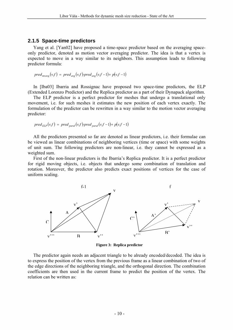
First of the non-linear predictors is the Ibarria’s Replica predictor. It is a perfect predictor for rigid moving objects, i.e. objects that undergo some combination of translation and rotation. Moreover, the predictor also predicts exact positions of vertices for the case of uniform scaling.
Figure 3: Replica predictor
The predictor again needs an adjacent triangle to be already encoded/decoded. The idea is
to express the position of the vertex from the previous frame as a linear combination of two of the edge directions of the neighboring triangle, and the orthogonal direction. The combination coefficients are then used in the current frame to predict the position of the vertex. The relation can be written as:
v’’’
v’
v’’
f-1 fv
v
v’’
v’
v’’’
A A’
B’
C’
B
C
Libor Váša - Methods for dynamic mesh size reduction - State of the Art
- 11 -
( ) ( )( ) ( )
( ) ( )( ) ( )( ) ( )
( ) ( ) CcBbAa,fv p v,fpred|BA|
BA C
,fv-p, fv p B, fv-p, fv p A
cCbB aA ,f-v-pv,f-pB||A
BA C
,f-v-p, f-v pB
replica ′+′+′+′′′=
′×′
′×′=′
′′′′′=′′′′′=′
++=′′′×
×=
′′′′′=
′′′′=
2
2
11
111-f ,vp-1-f ,vp A
Note that the normalization used in the computation of C and C’ ensures that the predictor
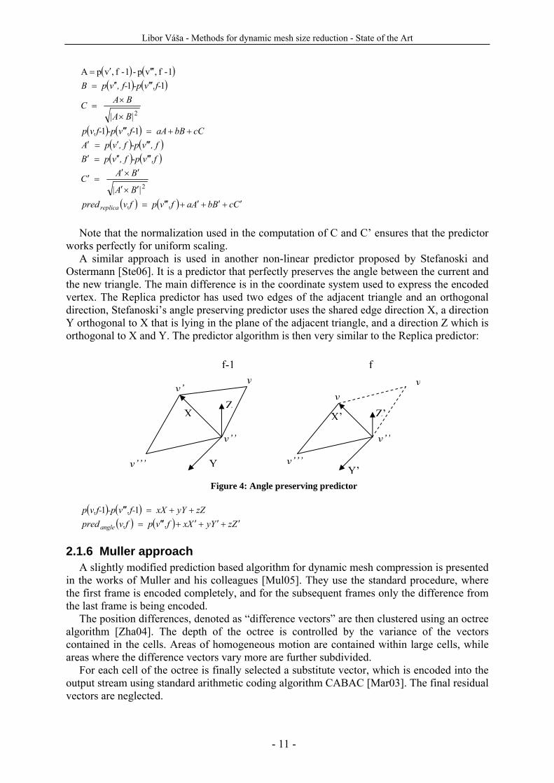
works perfectly for uniform scaling. A similar approach is used in another non-linear predictor proposed by Stefanoski and
Ostermann [Ste06]. It is a predictor that perfectly preserves the angle between the current and the new triangle. The main difference is in the coordinate system used to express the encoded vertex. The Replica predictor has used two edges of the adjacent triangle and an orthogonal direction, Stefanoski’s angle preserving predictor uses the shared edge direction X, a direction Y orthogonal to X that is lying in the plane of the adjacent triangle, and a direction Z which is orthogonal to X and Y. The predictor algorithm is then very similar to the Replica predictor:
Figure 4: Angle preserving predictor
( ) ( )
( ) ( ) ZzYyXx,fv p v,fpredzZyY xX ,f-v-pv,f-p
angle ′+′+′+′′′=++=′′′ 11
2.1.6 Muller approach A slightly modified prediction based algorithm for dynamic mesh compression is presented
in the works of Muller and his colleagues [Mul05]. They use the standard procedure, where the first frame is encoded completely, and for the subsequent frames only the difference from the last frame is being encoded.
The position differences, denoted as “difference vectors” are then clustered using an octree algorithm [Zha04]. The depth of the octree is controlled by the variance of the vectors contained in the cells. Areas of homogeneous motion are contained within large cells, while areas where the difference vectors vary more are further subdivided.
For each cell of the octree is finally selected a substitute vector, which is encoded into the output stream using standard arithmetic coding algorithm CABAC [Mar03]. The final residual vectors are neglected.
f-1 fv v
v’’v’’
v’
v’’’ v’’’
vX X’
Y Y’
Z’Z
Libor Váša - Methods for dynamic mesh size reduction - State of the Art
- 12 -
The method is inevitably lossy, information is lost when the whole cells of an octree are represented by a single substitute vector, which is moreover quantized. The amount of data loss can be steered by the depth of the constructed octree.
In their latest works[Mul07] the authors have enhanced the algorithm by introducing rate-distortion optimization. For each cell one of following predictors is chosen:
- direct coding – each vector is fully encoded - trilinear interpolation – eight corner vectors are encoded, the rest is interpolated. - mean replacement – uses the same idea of the original algorithm, i.e. replaces the
whole cell content by one substitute vector The decision about the predictor is made based upon the rate-distortion ratio for each cell. Generally, all the predictor based compression schemes provide an easy to implement and
very fast method for dynamic mesh compression. However, the spatio-temporal coherence that is present in the data is only exploited locally, by the predictor inputs. Generally, the fact that even distant parts of the object can behave in a similar way is not exploited by these algorithms. This issue has been addressed by the PCA based compression schemes, which will be described later in this chapter.
2.1.7 Wavelet based compression A wavelet base approach to dynamic mesh compression has been proposed by Payan in
[Pay05]. The method exploits temporal coherency of the data by iteratively dividing the sequence of vertex positions into high frequency and low frequency parts. The key observation is that for each frequency level a different quantizer can be used, i.e. each frequency can be encoded with different number of bits per sample. The authors propose to search for an optimal set of quantizers that produces the best rate/distortion ratio.
Because the method is aimed to exploit the temporal coherency of the input mesh, the wavelet encoding is applied on the trajectory of each vertex. The trajectory is represented by three sequences of values, each representing the evolution of one component of the position of the vertex in time. Each such sequence is encoded separately.
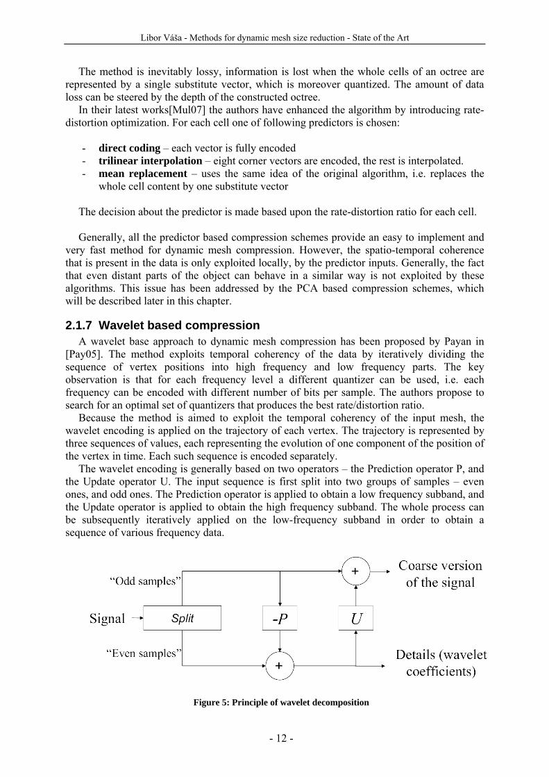
The wavelet encoding is generally based on two operators – the Prediction operator P, and the Update operator U. The input sequence is first split into two groups of samples – even ones, and odd ones. The Prediction operator is applied to obtain a low frequency subband, and the Update operator is applied to obtain the high frequency subband. The whole process can be subsequently iteratively applied on the low-frequency subband in order to obtain a sequence of various frequency data.
Figure 5: Principle of wavelet decomposition
Libor Váša - Methods for dynamic mesh size reduction - State of the Art
- 13 -
There are many P and U operators proposed in the literature, the authors state that they
have obtained best results using the [4,2] operator proposed in [Cal98]. The final step of the algorithm, which actually represents the compression of the data, is
the quantization. Each subband is compressed using different bitlength, and the optimal set of bitlengths is found using an iterative process with the constraint that the selected bitrate is matched.
2.1.8 PCA based compression A very interesting new approach to dynamic mesh compression has been introduced by
Alexa and Müller in 2000 [Ale00]. Their approach is completely different from the prediction based schemes presented above, as it uses principal component analysis (PCA) to determine a new basis for the animation. The compression is based on reducing the base size by omitting the basis elements of low importance.
The first step of the algorithm is to extract rigid motion from the animation, because rigid motion causes difficulties to the following PCA encoder. Each frame is moved so that its centre of mass lies in the origin, and an affine transformation of positive determinant is found which minimizes the squared distance from each vertex position to the corresponding vertex position in the first frame, thus removing any rotation and scaling motion that may be present in the animation. The coefficients of this transformation are then sent with each frame of the animation.
The process then continues with the PCA itself. Each frame of the animation is reordered to form a single column vector of length 3N (n being the number of vertices in each frame), i.e. all the X coordinates are stored first, followed by all the Y coordinates and all the Z coordinates. All the column vectors are ordered into a matrix B, which fully describes the animation. This matrix is now viewed as a set of samples in 3N-dimensional space. The task is to find such orthonormal basis of this 3N dimensional space, which is completely uncorrelated, i.e. where information about one component does not provide any information about any other component. The tool for finding such base is PCA, i.e. finding eigenvectors of the covariance matrix.
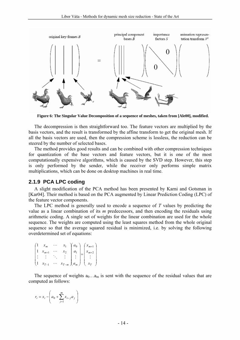
The authors propose to use the Singular Value Decomposition (SVD) to find the new basis for the space of frames. The SVD decomposes the matrix to following components:
TVSBB ⋅⋅= ˆ
Where B is the matrix of orthonormal principal component basis vectors, S is a diagonal
matrix of importance factors (in fact eigenvalues of B) and V is a matrix of animation representation transforms.
The rest of compression scheme is now straightforward. From the new basis we choose given number of vectors with highest importance factors and compute the representation Ef of each frame in this new reduced basis using the inner product:
( )n
Tff BBBBE ˆ,...,ˆ,ˆ
10⋅= where n is the selected number of basis vectors. The resulting vector of n components
(feature vector) is then sent with each frame. The last part of the encoded representation are the basis vectors themselves.
Libor Váša - Methods for dynamic mesh size reduction - State of the Art
- 14 -
Figure 6: The Singular Value Decomposition of a sequence of meshes, taken from [Ale00], modified.
The decompression is then straightforward too. The feature vectors are multiplied by the
basis vectors, and the result is transformed by the affine transform to get the original mesh. If all the basis vectors are used, then the compression scheme is lossless, the reduction can be steered by the number of selected bases.
The method provides good results and can be combined with other compression techniques for quantization of the base vectors and feature vectors, but it is one of the most computationally expensive algorithms, which is caused by the SVD step. However, this step is only performed by the sender, while the receiver only performs simple matrix multiplications, which can be done on desktop machines in real time.
2.1.9 PCA LPC coding A slight modification of the PCA method has been presented by Karni and Gotsman in
[Kar04]. Their method is based on the PCA augmented by Linear Prediction Coding (LPC) of the feature vector components.
The LPC method is generally used to encode a sequence of T values by predicting the value as a linear combination of its m predecessors, and then encoding the residuals using arithmetic coding. A single set of weights for the linear combination are used for the whole sequence. The weights are computed using the least squares method from the whole original sequence so that the average squared residual is minimized, i.e. by solving the following overdetermined set of equations:
⎟⎟⎟⎟⎟
⎠
⎞
⎜⎜⎜⎜⎜
⎝
⎛
=
⎟⎟⎟⎟⎟
⎠
⎞
⎜⎜⎜⎜⎜
⎝
⎛
⎟⎟⎟⎟⎟
⎠
⎞
⎜⎜⎜⎜⎜
⎝
⎛
+
+
−−
+
T
m
m
mmTT
m
m
x
xx
a
aa
xx
xxxx
MM
L
MOMM
L
L
2
1
1
0
1
21
1
1
11
The sequence of weights a0…am is sent with the sequence of the residual values that are
computed as follows:
⎟⎟
⎠
⎞
⎜⎜
⎝
⎛+−= ∑
=−
m
jjjiii axaxr
10
Libor Váša - Methods for dynamic mesh size reduction - State of the Art
- 15 -
The LPC coding can be used directly on dynamic meshes when each vertex trajectory is treated as a sequence of values, yielding sort of optimized temporal-only predictor encoding. However, such method would completely omit the strong spatial coherence that is usually present in dynamic meshes. The idea is to apply LPC to the animation at a point when the separate components of the representation are completely uncorrelated, i.e. after PCA.
The algorithm starts with finding the affine transform and PCA performed in the same manner as in [Ale00]. Subsequently, PCA is performed on the remaining non-rigid animation, and a subset of the basis is selected and feature vectors are computed. However, the feature vector components are not encoded directly, but using the LPC, each component of the vectors treated as a sequence of length equal to the length of the animation. The decompression is then also performed in a way similar to [Ale00], only the first step being the LPC decoding of the feature vectors.
The authors report reduction of the rate distortion ratio when compared to the PCA method only and when compared to the DynaPack method for animations of soft body movement, when the LPC of second or third order has been used.
2.1.10 Clustering based PCA encoding A further improvement of the PCA based encoding has been proposed in 2005 by Sattler et
al. [Sat05]. Their approach is based on reorganizing the data into a set of vertex paths instead of frames. PCA is subsequently applied on these paths, and the results of PCA are used to find a set of clusters of similar temporal behavior. These clusters are then encoded separately using the standard PCA method.
The data reorganization step is generally only a transposition of the B matrix from the original PCA-based encoding scheme. Subsequently, the clusters of locally linear behavior are found using following iterative process:
1. initialize k cluster centers randomly from the data set 2. associate each point to the closest cluster center according to a distance which is
evaluated as reconstruction error using center’s c most important eigenpaths 3. compute the new centers as mean of the data in each cluster 4. perform PCA again in each cluster 5. iterate the steps 2-4 until the average change in reconstruction error falls bellow
some given threshold. This process creates clusters of vertices, which move almost independently. These clusters
are subsequently encoded using the standard PCA-based encoder, i.e. by finding eigenshapes of each cluster and selecting a limited number of these which can be combined to approximate any shape from the input data.
The main drawback we have identified with this method is the iterative refinement initialization and the convergence speed. The random initialization causes the iterative process to converge to radically different solutions each time, and the convergence can take quite long time for moderately complex meshes. How to address this problem will be discussed in chapter 6.1.
Generally, all the current geometry compression schemes share one serious omission. They
all focus on minimizing the difference between the geometrical positions of vertices, while they don’t take the topology of the mesh into account. The last chapter of this material will give a suggestion about how we intend to address this problem.
Libor Váša - Methods for dynamic mesh size reduction - State of the Art
- 16 -
2.2 Triangular connectivity compression The usual way to describe connectivity of a triangular mesh is to store a table of index
triplets, where each triplet represents one triangle. Although intuitive, this approach has many drawbacks. On one hand, it does not explicitly store adjacency information, i.e. whenever there’s a need to obtain neighbors of given vertex or triangle, it is necessary to search the whole table. Moreover, such representation is very memory expensive, surprisingly even more expensive than the stored geometry information.
For simple mesh a so-called Euler equation holds:
2+=+ evf where f represents the number of faces (triangles), v is the number of vertices, and e is the
number of edges. From this equation follows that in a mesh there are about twice as many faces than vertices. We can express the space required to store geometry as
[ ]bitsvvG 96*3*32 ==
i.e. each vertex is represented by three 32 bit floating point numbers. The space required to
store the connectivity can be expressed as
⎡ ⎤ ⎡ ⎤ ⎡ ⎤[ ]bitsvvvvvfC 222 log6log**2*3log**3 === From the two equations one can derive that for a mesh of more than 216 = 65536 vertices
the connectivity information requires more space than the geometry. The following algorithms represent the state of the art in the lossless connectivity compression.
2.2.1 Topological Surgery Topological surgery is a static mesh connectivity compression algorithm proposed in 1998
by Taubin and Rossignac [Tau98]. In order to encode a mesh topology, it first cuts the original topology by a vertex spanning tree, which yields a set of triangle stripes (the best way to imagine this procedure is to see it as “peeling” the stripes from the original surface).
The resulting triangle tree is also encoded, along with a “march sequence” which encodes the topology of each triangle strip. The decompression algorithm first recovers the border of the cut mesh from the encoded vertex spanning tree, then it recovers the triangle stripes from the triangle spanning tree and the march sequences, and finally it sews the cuts and thus fully recovers the original topology. We will now describe each of the steps in more detail.
Libor Váša - Methods for dynamic mesh size reduction - State of the Art
- 17 -
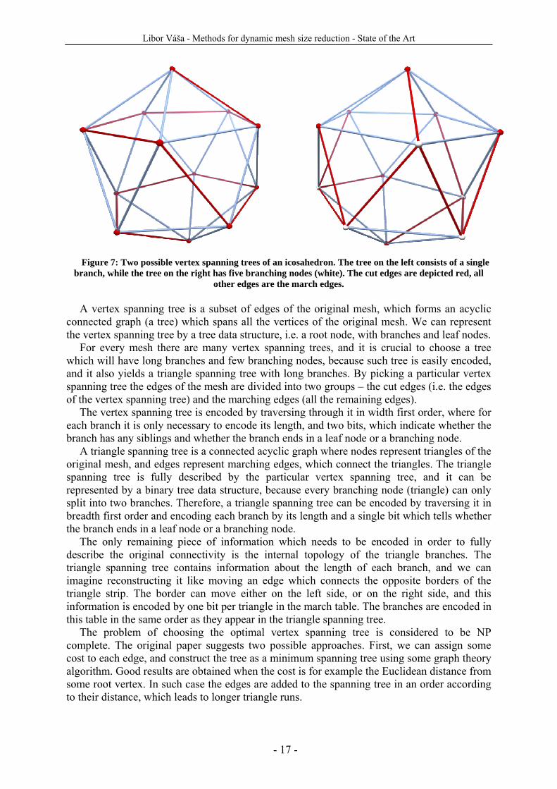
Figure 7: Two possible vertex spanning trees of an icosahedron. The tree on the left consists of a single branch, while the tree on the right has five branching nodes (white). The cut edges are depicted red, all
other edges are the march edges. A vertex spanning tree is a subset of edges of the original mesh, which forms an acyclic
connected graph (a tree) which spans all the vertices of the original mesh. We can represent the vertex spanning tree by a tree data structure, i.e. a root node, with branches and leaf nodes.
For every mesh there are many vertex spanning trees, and it is crucial to choose a tree which will have long branches and few branching nodes, because such tree is easily encoded, and it also yields a triangle spanning tree with long branches. By picking a particular vertex spanning tree the edges of the mesh are divided into two groups – the cut edges (i.e. the edges of the vertex spanning tree) and the marching edges (all the remaining edges).
The vertex spanning tree is encoded by traversing through it in width first order, where for each branch it is only necessary to encode its length, and two bits, which indicate whether the branch has any siblings and whether the branch ends in a leaf node or a branching node.
A triangle spanning tree is a connected acyclic graph where nodes represent triangles of the original mesh, and edges represent marching edges, which connect the triangles. The triangle spanning tree is fully described by the particular vertex spanning tree, and it can be represented by a binary tree data structure, because every branching node (triangle) can only split into two branches. Therefore, a triangle spanning tree can be encoded by traversing it in breadth first order and encoding each branch by its length and a single bit which tells whether the branch ends in a leaf node or a branching node.
The only remaining piece of information which needs to be encoded in order to fully describe the original connectivity is the internal topology of the triangle branches. The triangle spanning tree contains information about the length of each branch, and we can imagine reconstructing it like moving an edge which connects the opposite borders of the triangle strip. The border can move either on the left side, or on the right side, and this information is encoded by one bit per triangle in the march table. The branches are encoded in this table in the same order as they appear in the triangle spanning tree.
The problem of choosing the optimal vertex spanning tree is considered to be NP complete. The original paper suggests two possible approaches. First, we can assign some cost to each edge, and construct the tree as a minimum spanning tree using some graph theory algorithm. Good results are obtained when the cost is for example the Euclidean distance from some root vertex. In such case the edges are added to the spanning tree in an order according to their distance, which leads to longer triangle runs.
Libor Váša - Methods for dynamic mesh size reduction - State of the Art
- 18 -
Even better results are obtained with another sub optimal, but deterministic approach, called layered decomposition. This approach can be best imagined as literally peeling the triangles off the surface, starting at some given point. First, the triangles are divided into layers, according to their topological distance to some original triangle, i.e. all neighbors of the triangle are denoted as first layer, all neighbors of the first layer triangles are denoted as second layer etc.
Subsequently, the layers are converted to stripes, starting at the innermost. The stripes from each layer are constructed in a way that they ideally form a single long stripe. Using this technique, an example mesh of 5138 vertices mesh has been represented by 168 vertex runs.
Using the topological surgery approach, it is necessary to encode at least one bit per triangle for the march table, while the number of bits needed to encode the spanning trees vary according to how many branches are used. Using the layered decomposition the authors claim to achieve 2.16 bits per triangle for the sample mesh of 5138 vertices, while for very regular topology (for example obtained by some subdivision technique) the ratio can drop as low as 1.3 bits per triangle.
2.2.2 EdgeBreaker/cut-border machine A very elegant and simple way to efficiently encode connectivity of a triangular mesh has
been proposed in 1998 independently by Gumhold and Straßer ([Gum98]) and Rossignac ([Ros99]). In this text we will describe the Rossignac’s EdgeBreaker algorithm, which provides some advantages over the slightly earlier Cut-border machine proposed by Gumhold and Straßer.
The basic idea of the algorithm is to encode a traversal through all the triangles of the mesh. For simplicity we describe only the basic version of the algorithm, which works for a simple mesh.
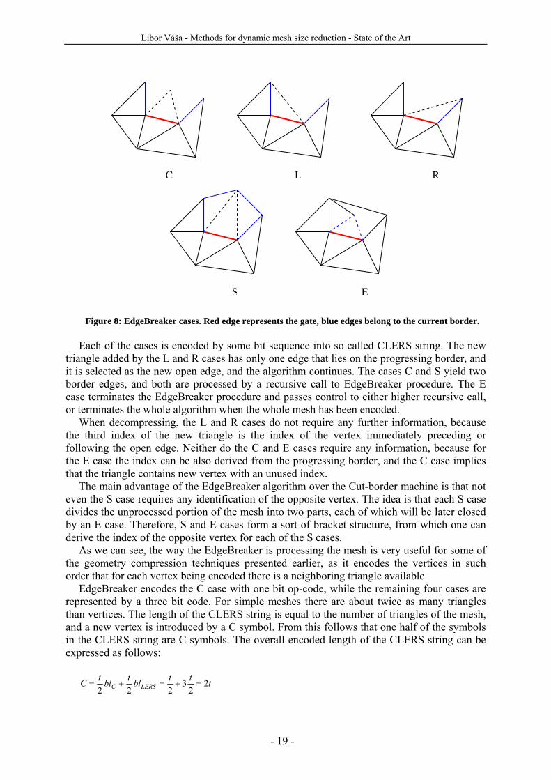
The first triangle is encoded in full, and its edges form the first progressing border. One of the edges of the initial triangle is selected as “open”, and it will be used to grow the progressing border. The open edge connects the current triangle with exactly one new triangle, which contains the open edge and one more triangle. There are five possible cases for the vertex:
1) it is a new one, which has not been touched by the progressing border yet (case C) 2) it is a vertex that lies on the progressing border immediately to the left of the open
edge (case L) 3) it is a vertex that lies on the progressing border immediately to the right of the open
edge (case R) 4) it is a vertex that lies on the progressing border both immediately to the left and to the
right, i.e. it closes a single triangle hole in the mesh (case E) 5) it is a vertex which lies on the progressing border, but somewhere else that
immediately to the left or right (case S)
Libor Váša - Methods for dynamic mesh size reduction - State of the Art
- 19 -
Figure 8: EdgeBreaker cases. Red edge represents the gate, blue edges belong to the current border.
Each of the cases is encoded by some bit sequence into so called CLERS string. The new
triangle added by the L and R cases has only one edge that lies on the progressing border, and it is selected as the new open edge, and the algorithm continues. The cases C and S yield two border edges, and both are processed by a recursive call to EdgeBreaker procedure. The E case terminates the EdgeBreaker procedure and passes control to either higher recursive call, or terminates the whole algorithm when the whole mesh has been encoded.
When decompressing, the L and R cases do not require any further information, because the third index of the new triangle is the index of the vertex immediately preceding or following the open edge. Neither do the C and E cases require any information, because for the E case the index can be also derived from the progressing border, and the C case implies that the triangle contains new vertex with an unused index.
The main advantage of the EdgeBreaker algorithm over the Cut-border machine is that not even the S case requires any identification of the opposite vertex. The idea is that each S case divides the unprocessed portion of the mesh into two parts, each of which will be later closed by an E case. Therefore, S and E cases form a sort of bracket structure, from which one can derive the index of the opposite vertex for each of the S cases.
As we can see, the way the EdgeBreaker is processing the mesh is very useful for some of the geometry compression techniques presented earlier, as it encodes the vertices in such order that for each vertex being encoded there is a neighboring triangle available.
EdgeBreaker encodes the C case with one bit op-code, while the remaining four cases are represented by a three bit code. For simple meshes there are about twice as many triangles than vertices. The length of the CLERS string is equal to the number of triangles of the mesh, and a new vertex is introduced by a C symbol. From this follows that one half of the symbols in the CLERS string are C symbols. The overall encoded length of the CLERS string can be expressed as follows:
tttbltbltC LERSC 2
23
222=+=+=
C L R
S E
Libor Váša - Methods for dynamic mesh size reduction - State of the Art
- 20 -
where C represents the encoded length of connectivity, blC stands for bit length of C code and blLERS represents the bit length of codes L, E, R and S. In other words, it is guaranteed that for a simple mesh the connectivity is compressed to a maximum of 2 bits per triangle.
In practice using arithmetic coding on the CLERS sequence yields about 1.7 bits per triangle, or even less than that for extremely regular connectivity meshes. This property will be later exploited by the SwingWrapper remeshing algorithm described in chapter 3.1.2.
2.2.3 Delphi geometry based connectivity encoding A very elegant improvement of the EdgeBreaker algorithm has been recently proposed by
Coors and Rossignac[Coo99]. The idea is to combine some of the geometry estimators and the EdgeBreaker algorithm. The geometry predictor is used to predict the position of the next vertex, and a threshold algorithm is used to deduce a guess about what of the CLERS cases occurs. As both the encoder and decoder use the same estimator, it suffices to send a single confirmation bit instead of one of the CLERS op-codes.
However, the performance of the algorithm depends on the accuracy of the CLERS predictor, which depends on the used geometry prediction. The authors of Delphi have used the parallelogram predictor, and they report that for usual meshes they have achieved guess accuracy over 80%, which lead to compression to about 1.3-1.5 bits per triangle
2.3 Tetrahedral connectivity compression We will now describe two methods for tetrahedral connectivity compression. The
relevance of tetrahedral meshes to dynamic mesh data rate reduction will be justified in the following text.
From Euler equation for triangular meshes follows that the average vertex-triangle order of a low Euler characteristic mesh is 6. Unfortunately, for the case of tetrahedral meshes this does not hold, there are some pathological cases with extreme vertex-tetrahedron order, and even for the meshes usually used in computer graphics or data processing is the vertex-tetrahedron order more variable than in the case of triangular meshes. For example a regular cubic lattice subdivided by the 5 tetrahedra scheme leads to vertex-tetrahedron order 12, while using the 6 tetrahedra scheme produces vertices of average order 14.
The authors of [Gum99] specify the expected relations in a usual tetrahedral mesh as follows:
5.5:11:6.5:1 =v:e:f:t
where v is the number of vertices, e is the number of edges, f is the number of faces and t is
the number of tetrahedra.
2.3.1 Grow&Fold On of the first efforts on the field of tetrahedral mesh connectivity compression is the
Grow&Fold algorithm published by Szymczak and Rossignac [Szy99]. It is based on a combination of ideas of the EdgeBreaker and topological surgery algorithms for triangle mesh compression. The algorithm is able to compress the connectivity of a tetrahedral mesh from 128 bits per tetrahedron (four 32-bit indices per tetrahedron) down to a little over 7 bits per tetrahedron.
The first step is similar to building of triangle spanning tree in the topological surgery approach, only this time a tetrahedron spanning tree is constructed. An arbitrary border triangle is selected as a “root door”, which leads to the first tetrahedron of the tree. Each tetrahedron adds three new doors, which correspond to the tree new triangles that together
Libor Váša - Methods for dynamic mesh size reduction - State of the Art
- 21 -
with the current door form the given tetrahedron. Each of the doors is then processed in a specific order.
The tetrahedron spanning tree is encoded by three bits per tetrahedron, where the bits declare whether each of the triangles is a “door” to a new branch of the tree or not. The decoder is then able to “grow” the tree by processing the string of encoded tetrahedra. However, this step only reconstructs the connectivity partially, it is necessary to connect the branches of the tree to reconstruct the geometry of the original tetrahedral mesh.
The authors recognize two ways to connect tetrahedra in the tree. First, the “fold” operation connects the tetrahedron to one of its current neighbors, similar to L or R states in the EdgeBreaker algorithm. Each “cut” face, i.e. every face of the grown tetrahedral spanning tree, is assigned a two-bit code, which tells the decoder which one of the edges is the “fold edge”, or tells the decoder that no fold operation should be performed upon the given face. There are 2t+1 external faces of the tetrahedron spanning tree, and therefore there are 4t+2 bits needed to encode the “folding string”, in which the faces are encoded in the same order in which the tetrahedra are processed by the spanning tree construction algorithm.
After the folding of the tree it is still possible that some of the faces that are supposed to be connected are not connected, this case occurs when a face is adjacent to a tetrahedron which is not adjacent in the tetrahedron spanning tree. Such case is solved by the “glue” operation, which is the only one which needs an explicit index, which tells what faces should be glued. It is shown that for reasonable meshes the number of required glue operations is low, and therefore it does not influence the overall performance of the algorithm, which remains at 7 bits per tetrahedron.
2.3.2 Cut-border The cut-border machine for triangular connectivity compression is in contrast with the
Edgebreaker algorithm easily extendable to the case of tetrahedral connectivity compression problem. The extension has been proposed in 1999 by Gumhold and Straßer [Gum99].
The cut-border is a triangle mesh, which divides the tetrahedral mesh into two parts, inner and outer. This border is initialized to a single tetrahedron, and it is grown until it is equal to the border of the whole tetrahedral mesh. The growing of the cut border is performed by processing one triangle of the border at a time, where order of processing of triangles is set by a strategy which will be described later.
There are three basic situations, in which can a cut-border triangle be. It can either be a border triangle, it can be a base of a tetrahedron formed by a new vertex, or it can be a base of a tetrahedron formed by one of the cut-border vertices. Each of these cases is encoded into an output stream, the authors of [Gum99] denote the states as ∆ (close), * (new vertex) and ∞ (connect). Of these only the ∞ needs a parameter, which will tell the decoder which of the cut-border vertices should be used to form a new tetrahedron. The ∆ and * operations do not need any extra information.
In order to improve the compression rate, it is useful to use local indices as parameters of the ∞ operation. Such local indices are created in a way that the nearest vertices have the lowest numbers. One of the edges of the cut-border triangles is selected to be the “zero edge”. All the vertices are then searched in the breadth-first order from this edge, until the incident vertex is reached. The order in which it has been found is then encoded as the index for the ∞ operation.
The created sequence of close, new vertex and connect operations is then used by the decompressing algorithm to reconstruct the original connectivity. It is possible that during the decompression the cut-border represents a non-manifold mesh; however the final state of the cut border is guaranteed to be equal to the border of the original tetrahedral mesh.
Libor Váša - Methods for dynamic mesh size reduction - State of the Art
- 22 -
In order to reduce the number of connect operations with high index, the authors propose to process vertices of the original mesh in a fifo order, while all the cut-border triangles incident with current vertex are processed before the algorithm continues to another vertex. This rule represents one possible strategy for choosing a cut-border triangle.
The choice of zero-edge also influences the number of high index connect operations, the proposed strategy is to set the zero edge for each triangle at the time it is added to the cut border, and set it to the edge that this triangle shares with the triangle which caused its insertion.
The cut-border machine is able to reduce the cost of connectivity compression for tetrahedral mesh from theoretical value
⎡ ⎤vtC 2log4=
down to about 11 bits per vertex, i.e. about 2 bits per tetrahedron.
Libor Váša - Methods for dynamic mesh size reduction - State of the Art
- 23 -
3 Simplification Triangular mesh simplification is one of the most intensively studied problems of computer
graphics. In contrast to compression, simplification always changes the topology of the data, and therefore it almost always changes the shape of the data. From our point of view this represents no problem, as we aim to produce shapes that are visually similar, but not necessarily equal to the input.
There are approaches to various special cases of the problem, however we will only focus on main directions applicable to triangular and tetrahedral meshes. For a deeper review of existing simplification methods see [Fra02], [Got02], [All05].
In the following text we will describe the basic approaches to simplification methods based on vertex removal, edge collapsing, remeshing and geometry images, which is of particular interest for us, because it can be extended to t-variant case in the form of geometry video. We will also give details about tetrahedral mesh simplification methods, because we will show in the last section that a dynamic 3D mesh can be represented by a static 4D tetrahedral mesh.
3.1 Triangular simplification
3.1.1 Schroeder decimation The algorithm proposed by Schroeder in [Sch92] works on triangular meshes and is based
on vertex removal and retriangulation of the hole. Such approach is known as mesh decimation, and its results strongly depend on the decimation criterion used.
The algorithm works in three steps, which are iteratively repeated until the desired simplification ratio is reached. These steps are
1. characterize the local vertex geometry and topology 2. evaluate the decimation criteria 3. remove vertices and retriangulate the holes
The original algorithm takes into account so-called feature edges, i.e. edges of angle higher
than given threshold. Such edges are considered important, and the algorithm tries to preserve them. The feature edges form a geometrical characteristic, which must be evaluated along with the topological characteristic of vertex surroundings. We can distinguish following cases:
- simple vertex (its neighborhood is topologically equivalent to a disc, it does not incide with any feature edges)
- complex vertex (a non-manifold vertex, cannot occur with our inputs) - boundary vertex (incides with two border edges) - interior edge vertex (incides with exactly two feature edges) - corner vertex (incides with three or more feature edges)
Libor Váša - Methods for dynamic mesh size reduction - State of the Art
- 24 -
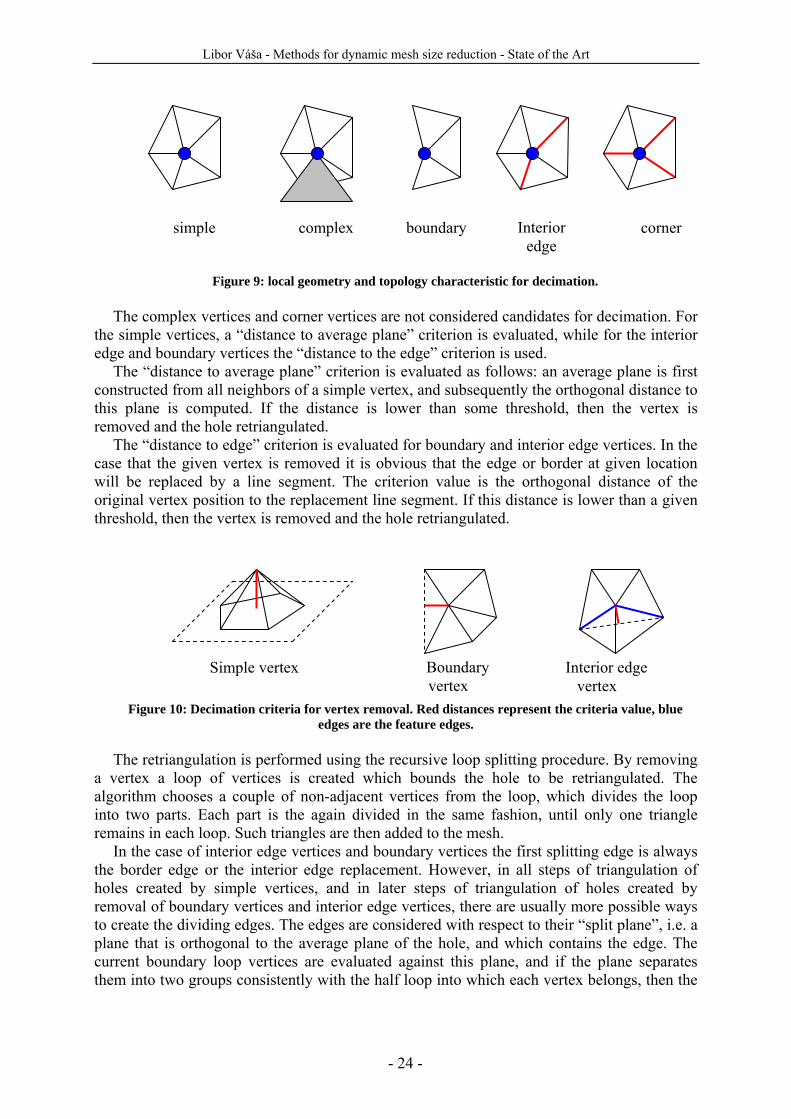
Figure 9: local geometry and topology characteristic for decimation.
The complex vertices and corner vertices are not considered candidates for decimation. For
the simple vertices, a “distance to average plane” criterion is evaluated, while for the interior edge and boundary vertices the “distance to the edge” criterion is used.
The “distance to average plane” criterion is evaluated as follows: an average plane is first constructed from all neighbors of a simple vertex, and subsequently the orthogonal distance to this plane is computed. If the distance is lower than some threshold, then the vertex is removed and the hole retriangulated.
The “distance to edge” criterion is evaluated for boundary and interior edge vertices. In the case that the given vertex is removed it is obvious that the edge or border at given location will be replaced by a line segment. The criterion value is the orthogonal distance of the original vertex position to the replacement line segment. If this distance is lower than a given threshold, then the vertex is removed and the hole retriangulated.
Figure 10: Decimation criteria for vertex removal. Red distances represent the criteria value, blue
edges are the feature edges. The retriangulation is performed using the recursive loop splitting procedure. By removing
a vertex a loop of vertices is created which bounds the hole to be retriangulated. The algorithm chooses a couple of non-adjacent vertices from the loop, which divides the loop into two parts. Each part is the again divided in the same fashion, until only one triangle remains in each loop. Such triangles are then added to the mesh.
In the case of interior edge vertices and boundary vertices the first splitting edge is always the border edge or the interior edge replacement. However, in all steps of triangulation of holes created by simple vertices, and in later steps of triangulation of holes created by removal of boundary vertices and interior edge vertices, there are usually more possible ways to create the dividing edges. The edges are considered with respect to their “split plane”, i.e. a plane that is orthogonal to the average plane of the hole, and which contains the edge. The current boundary loop vertices are evaluated against this plane, and if the plane separates them into two groups consistently with the half loop into which each vertex belongs, then the
simple complex boundary Interior edge
corner
Simple vertex Boundary vertex
Interior edge vertex
Libor Váša - Methods for dynamic mesh size reduction - State of the Art
- 25 -
given edge is accepted as possible split edge. If no acceptable split edge is found, then the vertex is not removed from the mesh.
Still, there may be multiple possible split edges. For each such edge an aspect ratio criterion is evaluated. This criterion is constructed to prefer short edges that well separate the edges of the hole. Let’s denote the minimum distance of the loop edges to the split plane dmin, and the length of the edge l. The aspect ratio is then simply expressed as
ldCaspect
min=
In order to get best results is the value of the criterion limited by some threshold, and if no
edge is found to provide sufficient criterion value, then the vertex is again not removed. This simplification scheme is very simple and has been extended to cover various special
cases and provide better results by using different criteria. Various speedup techniques have been also proposed in order to avoid sorting the candidate vertices in each step of the algorithm [Fra01]. However, the method only uses the vertex positions of the original mesh, even in cases when it could be beneficial to move the vertices to new positions in order to better fit the original shape.
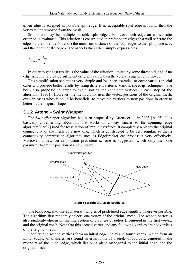
3.1.2 Attene – SwingWrapper The SwingWrapper algorithm has been proposed by Attene et al. in 2003 [Att03]. It is
basically a remeshing algorithm that works in a way similar to the spinning edge algorithm[Čer02] used for tessellation of implicit surfaces. It completely replaces the original connectivity of the mesh by a new one, which is constructed to be very regular, so that a connectivity compression algorithm such as EdgeBreaker can process it very effectively. Moreover, a new vertex position prediction scheme is suggested, which only uses one parameter to set the position of a new vertex.
dihedral angle
predicted vertex position
actual vertex position
gate edge
Figure 11: Dihedral angle predictor. The basic idea is to use equilateral triangles of predefined edge length L wherever possible.
The algorithm first randomly selects one vertex of the original mesh. The second vertex is also randomly chosen on the intersection of a sphere of radius L centered in the first vertex, and the original mesh. Note that this second vertex and any following vertices are not vertices of the original mesh.
The first and second vertices form an initial edge. Third and fourth vertex, which form an initial couple of triangles, are found as crosspoints of a circle of radius L centered in the midpoint of the initial edge, which lies on a plane orthogonal to the initial edge, and the original mesh.
Libor Váša - Methods for dynamic mesh size reduction - State of the Art
- 26 -
The open edges of the initial couple of triangles form four initial gates, from which a combination of remeshing algorithm and EdgeBreaker algorithm starts an iterative processing of the mesh. During this process, a new triangular mesh M’ is created from the original mesh M.
A midpoint of the gate is selected, a circle of radius L centered at the midpoint and lying on a plane orthogonal to the gate is constructed, and intersection with the original mesh is found.
The intersection point which is further from the base of the gate is selected. If it is closer to any existing vertex of M’ than one half of the L length, then it is snapped to this vertex by encoding one of the LERS EdgeBreaker codes. If the new vertex is not snapped to any existing vertex, then the C case is encoded, along with geometry specification of the new vertex.
The encoding of a new vertex is performed in a way which exploits the regularity of the mesh. The so-called dihedral angle scheme is used to encode the position of the new vertex. The decoder knows that the new vertex lies on a circle centered in the mid-point of the gate, and can guess its position to be on the plane of the gate triangle. The only correcting information is the angle between the guessed position of the new vertex, and its real position, i.e. a single number, which is claimed to be sufficiently quantized to 8 bits, given that both decoder and encoder use the quantized positions, so that the error does not propagate and accumulate.
The overall size of the encoded mesh can be easily computed as
ttvCGE 628 =+=+= where E stands for the encoded length of the mesh, G stands for encoded length of
geometry and C stands for the length of encoded connectivity. We can also estimate the dependency of the number of triangles of M’ on the selected length L:
432L
At =
where A stands for the area of the original mesh M. Given these relations, we can easily
steer the compression to produce compressed representation of desired length. Using some advanced arithmetic compression technique can bring the encoding cost even lower down to about 4 bits per triangle.
There are two main drawbacks of this approach. First, the created mesh is very regular, and it does not use the local properties of the input mesh, i.e. even very flat regions of the original mesh will be sampled with constant density.
Libor Váša - Methods for dynamic mesh size reduction - State of the Art
- 27 -
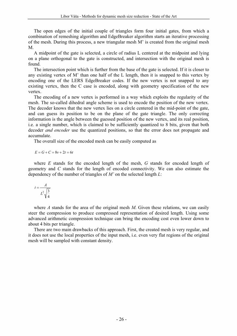
Figure 12: Smoothing effect of the SwingWrapper remeshing. Taken form [Att03].
The other drawback is that the method performs some smoothing of the original mesh,
which is also caused by the fact that it does not adapt to local changes in the mesh curvature. This feature could be solved by some adaptive technique known from implicit function tessellation, but this would make the encoding more complex and in effect less efficient.
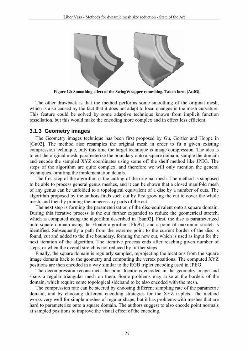
3.1.3 Geometry images The Geometry images technique has been first proposed by Gu, Gortler and Hoppe in
[Gu02]. The method also resamples the original mesh in order to fit a given existing compression technique, only this time the target technique is image compression. The idea is to cut the original mesh, parameterize the boundary onto a square domain, sample the domain and encode the sampled XYZ coordinates using some off the shelf method like JPEG. The steps of the algorithm are quite complex, and therefore we will only mention the general techniques, omitting the implementation details.
The first step of the algorithm is the cutting of the original mesh. The method is supposed to be able to process general genus meshes, and it can be shown that a closed manifold mesh of any genus can be unfolded to a topological equivalent of a disc by a number of cuts. The algorithm proposed by the authors finds such cut by first growing the cut to cover the whole mesh, and then by pruning the unnecessary parts of the cut.
The next step is forming the parameterization of the disc-equivalent onto a square domain. During this iterative process is the cut further expanded to reduce the geometrical stretch, which is computed using the algorithm described in [San02]. First, the disc is parameterized onto square domain using the Floater algorithm [Flo97], and a point of maximum stretch is identified. Subsequently a path from the extreme point to the current border of the disc is found, cut and added to the disc boundary, forming the new cut, which is used as input for the next iteration of the algorithm. The iterative process ends after reaching given number of steps, or when the overall stretch is not reduced by further steps.
Finally, the square domain is regularly sampled, reprojecting the locations from the square image domain back to the geometry and computing the vertex positions. The computed XYZ positions are then encoded in a way similar to the RGB triplet encoding used in JPEG.
The decompression reconstructs the point locations encoded in the geometry image and spans a regular triangular mesh on them. Some problems may arise at the borders of the domain, which require some topological sideband to be also encoded with the mesh.
The compression rate can be steered by choosing different sampling rate of the parametric domain, and by choosing different encoding strategies for the XYZ triplets. The method works very well for simple meshes of regular shape, but it has problems with meshes that are hard to parameterize onto a square domain. The authors suggest to also encode point normals at sampled positions to improve the visual effect of the encoding.
Libor Váša - Methods for dynamic mesh size reduction - State of the Art
- 28 -
Figure 13: Examples of geometry images. The top row shows the cut, the bottom row shows the
resulting geometry images. The image has been taken from [Gu02].
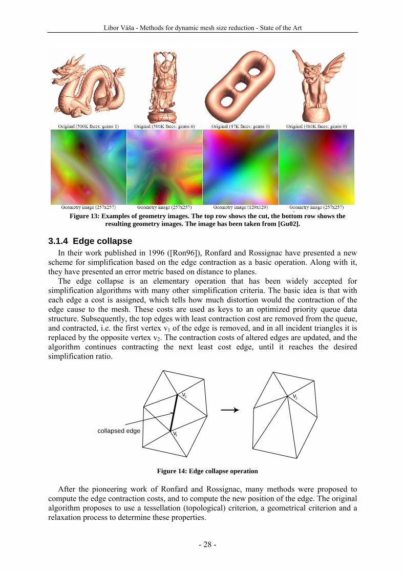
3.1.4 Edge collapse In their work published in 1996 ([Ron96]), Ronfard and Rossignac have presented a new
scheme for simplification based on the edge contraction as a basic operation. Along with it, they have presented an error metric based on distance to planes.
The edge collapse is an elementary operation that has been widely accepted for simplification algorithms with many other simplification criteria. The basic idea is that with each edge a cost is assigned, which tells how much distortion would the contraction of the edge cause to the mesh. These costs are used as keys to an optimized priority queue data structure. Subsequently, the top edges with least contraction cost are removed from the queue, and contracted, i.e. the first vertex v1 of the edge is removed, and in all incident triangles it is replaced by the opposite vertex v2. The contraction costs of altered edges are updated, and the algorithm continues contracting the next least cost edge, until it reaches the desired simplification ratio.
collapsed edge v
v
1
2 v2
Figure 14: Edge collapse operation
After the pioneering work of Ronfard and Rossignac, many methods were proposed to compute the edge contraction costs, and to compute the new position of the edge. The original algorithm proposes to use a tessellation (topological) criterion, a geometrical criterion and a relaxation process to determine these properties.
Libor Váša - Methods for dynamic mesh size reduction - State of the Art
- 29 -
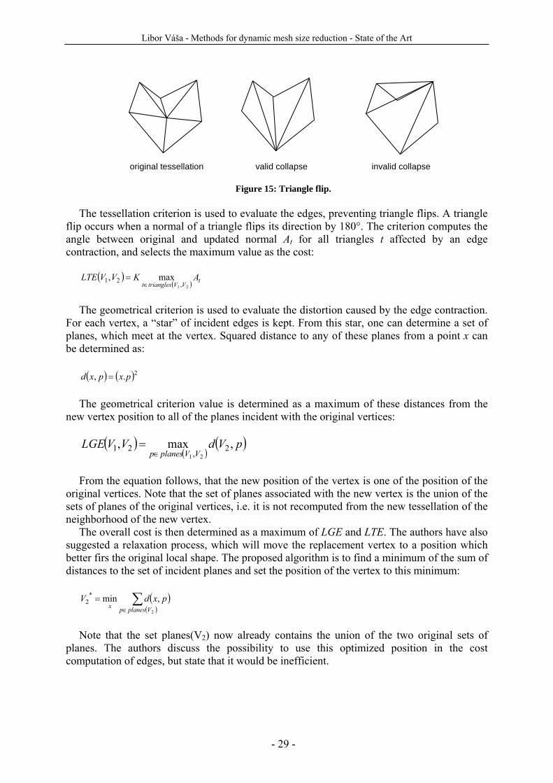
original tessellation valid collapse invalid collapse
Figure 15: Triangle flip.
The tessellation criterion is used to evaluate the edges, preventing triangle flips. A triangle flip occurs when a normal of a triangle flips its direction by 180°. The criterion computes the angle between original and updated normal At for all triangles t affected by an edge contraction, and selects the maximum value as the cost:
( )
( ) tVVtrianglest
AKVVLTE21 ,
21 max,∈
=
The geometrical criterion is used to evaluate the distortion caused by the edge contraction.
For each vertex, a “star” of incident edges is kept. From this star, one can determine a set of planes, which meet at the vertex. Squared distance to any of these planes from a point x can be determined as:
( ) ( )2., pxpxd =
The geometrical criterion value is determined as a maximum of these distances from the
new vertex position to all of the planes incident with the original vertices:
( )( )
( )pVdVVLGEVVplanesp
,max, 2,
2121∈
=
From the equation follows, that the new position of the vertex is one of the position of the
original vertices. Note that the set of planes associated with the new vertex is the union of the sets of planes of the original vertices, i.e. it is not recomputed from the new tessellation of the neighborhood of the new vertex.
The overall cost is then determined as a maximum of LGE and LTE. The authors have also suggested a relaxation process, which will move the replacement vertex to a position which better firs the original local shape. The proposed algorithm is to find a minimum of the sum of distances to the set of incident planes and set the position of the vertex to this minimum:
( )
( )∑
∈
=2
,min*2
VplanespxpxdV
Note that the set planes(V2) now already contains the union of the two original sets of
planes. The authors discuss the possibility to use this optimized position in the cost computation of edges, but state that it would be inefficient.
Libor Váša - Methods for dynamic mesh size reduction - State of the Art
- 30 -
3.1.5 Quadric based The quadric based simplification method proposed by Garland in 1997 ([Gar97]) is based
on the pair contraction technique, which is similar to edge contraction, and its main contribution is a novel method of evaluating the pairs for contraction.
The concept of pair contraction is a simple augmentation of the edge contraction described above. The difference is that a pair can be either an edge, or a couple of vertices which is not connected by an edge, but which is very close together. Using the pair contraction instead of edge contraction allows simplification of topology of the mesh, i.e. connecting previously unconnected components of the mesh.
The algorithm works in five steps: 1. select valid pairs for contraction 2. evaluate the pairs (see below) 3. sort the pairs according to their evaluation 4. iteratively contract the pairs and update the mesh
The key step is the evaluation of pairs. First, we will describe the situation at one vertex. A
vertex is an intersection of planes, in which lie the incident triangles. If we want express the squared distance of a point x from a plane p, we use a simple dot product:
( ) ( )2pxxd T
p = where x is the position represented in homogeneous coordinates and p is the vector of
coefficients of the implicit plane equation. If we now want to express the squared distance from a set of planes incident with some vertex v, we simply add the distances together:
( ) ( )
( )∑
∈
=vplanesp
Tv pxxd
2
The sum can be rewritten as follows:
( ) ( )( )( )
( )( )
( )
Qxx
xppx
xppx
xppxxd
T
vplanesp
TT
vplanesp
TT
vplanesp
TTv
=
⎟⎟
⎠
⎞
⎜⎜
⎝
⎛=
=
=
∑
∑
∑
∈
∈
∈
From the last expression follows, that computing sum of squared distances from a set of
planes incident with a given vertex can be expressed by a quadratic form. This form can be pre-computed for each vertex of the original mesh. When a pair is considered for contraction, then the quadrics of its endpoints are simply added together. The final position after the contraction is found by minimizing the error measure. The minimum is found by finding the zero point of the first derivative of the quadric form, i.e. by solving the following set of equations:
Libor Váša - Methods for dynamic mesh size reduction - State of the Art
- 31 -
⎥⎥⎥⎥
⎦
⎤
⎢⎢⎢⎢
⎣
⎡
=
⎥⎥⎥⎥
⎦
⎤
⎢⎢⎢⎢
⎣
⎡
1000
1000
*
34333231
24232221
14131211
xqqqqqqqqqqqq
where qxy are elements of the summed quadric Q12 = Qv1+Qv2. Note that the last line of the
matrix expresses that we are looking for a solution with homogeneous coordinate equal to 1. The overall error measure for given pair is expressed as
*
12* xQxp T=
This measure is then used to sort the pairs, and the pairs of lowest error measure are
contracted first.
3.1.6 Locally volume preserving edge collapse All the edge collapse criteria presented so far were based on the idea that the new cost
should be computed with respect to the original mesh. Lindstrom and Turk in their work [Lin98] have dropped this assumption, and their algorithm only uses the current simplified version of the mesh to compute the costs of contraction of each edge. Their criterion is based on local volume preservation, which leads to global volume preservation, which is a problem for some simple vertex placement schemes, including the original one presented in [Ron96]. We will first describe the algorithm that sets the position of the new vertex after edge collapse, and then we will show a cost function which is closely related to it.
The new vertex position is set by searching for an intersection of three planes, each of which represents some constraint about the position of the vertex. The authors provide equations for several possible constraints, and propose an ordering in which these constraints are evaluated, and their planes constructed. It is possible that some of the constraints produce planes that are almost coplanar, i.e. an underdetermined system which is easily disturbed by rounding errors. Such case is detected by checking the angle between the planes. Cases when the angle is lower than 1° are called α incompatible and the next constraint from the priority ordering is selected. The possible constraints are (in order in which they are evaluated):
1) volume preservation 2) boundary preservation 3) volume optimization 4) boundary optimization 5) triangle shape optimization The volume preservation constraint enforces that the volume is not changed after the edge
is collapsed. The space between the original and new tessellation of the neighborhood of the collapsed edge is divided to tetrahedra, each having base in one of the original triangles, and a top in the new vertex. A signed volume of a tetrahedron can be expressed as:
( )
111161
210
210
210
zzzz
yyyy
xxxx
vvvvvvvvvvvv
tV =
Where v is the location of the top of the tetrahedron, and v0, v1 and v2 are vertices of its base. Note that this volume is negative when the top is located below the base with respect to
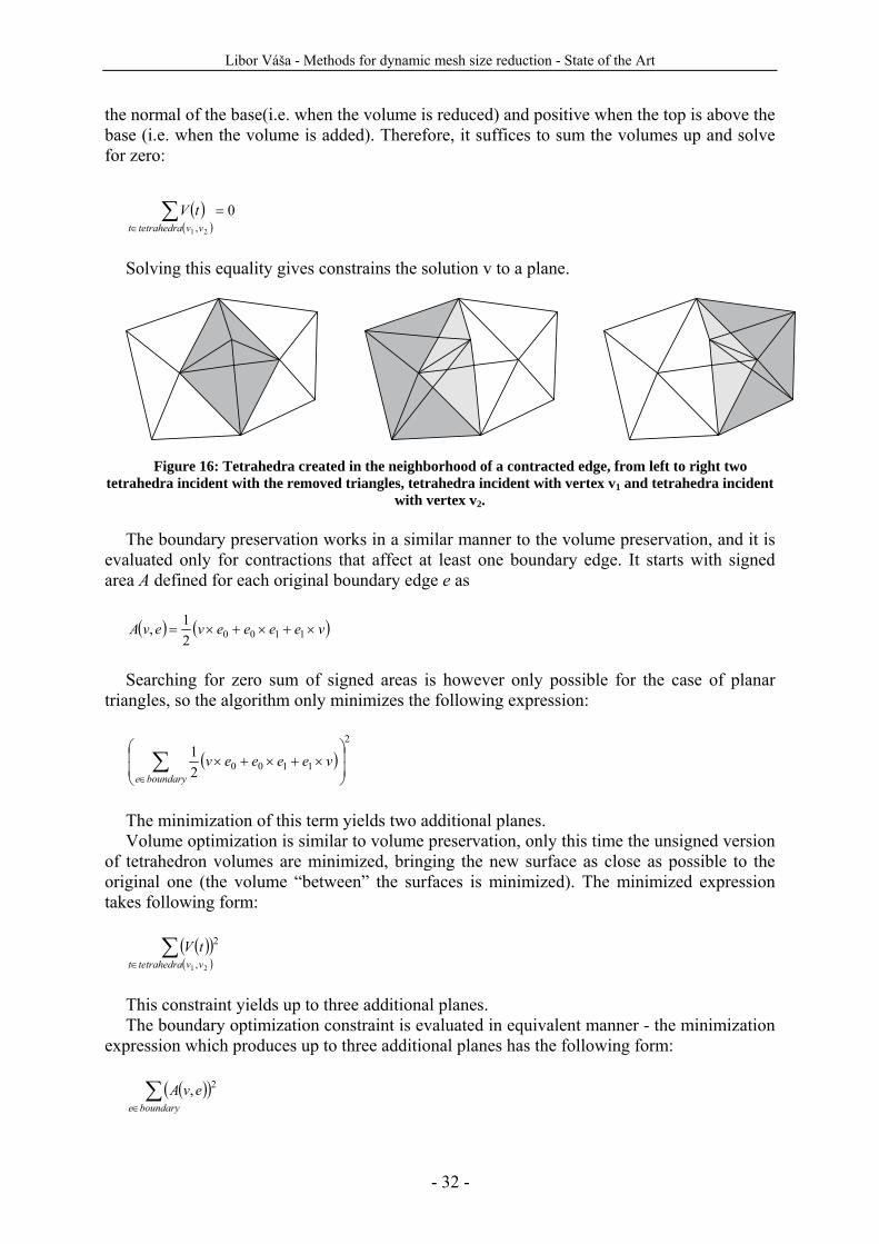
Libor Váša - Methods for dynamic mesh size reduction - State of the Art
- 32 -
the normal of the base(i.e. when the volume is reduced) and positive when the top is above the base (i.e. when the volume is added). Therefore, it suffices to sum the volumes up and solve for zero:
( )( )
021 ,=∑
∈ vvtetrahedrattV
Solving this equality gives constrains the solution v to a plane.
Figure 16: Tetrahedra created in the neighborhood of a contracted edge, from left to right two tetrahedra incident with the removed triangles, tetrahedra incident with vertex v1 and tetrahedra incident
with vertex v2.
The boundary preservation works in a similar manner to the volume preservation, and it is evaluated only for contractions that affect at least one boundary edge. It starts with signed area A defined for each original boundary edge e as
( ) ( )veeeevevA ×+×+×= 11002
1,
Searching for zero sum of signed areas is however only possible for the case of planar
triangles, so the algorithm only minimizes the following expression:
( )2
110021
⎟⎟
⎠
⎞
⎜⎜
⎝
⎛×+×+×∑
∈boundaryeveeeev
The minimization of this term yields two additional planes. Volume optimization is similar to volume preservation, only this time the unsigned version
of tetrahedron volumes are minimized, bringing the new surface as close as possible to the original one (the volume “between” the surfaces is minimized). The minimized expression takes following form:
( )( )
( )∑
∈ 21 ,
2
vvtetrahedrattV
This constraint yields up to three additional planes. The boundary optimization constraint is evaluated in equivalent manner - the minimization
expression which produces up to three additional planes has the following form:
( )( )∑∈boundarye
evA 2,
Libor Váša - Methods for dynamic mesh size reduction - State of the Art
- 33 -
The triangle shape optimization constraint is only used in the case when the previous constraints have not produced three α -compatible planes. This case usually occurs when the triangles of the original mesh are almost coplanar. In such case, the last constraint simply prefers equilateral triangles to long ones. The minimized expression is:
( )( )∑
iivvL 2,
Where L is the distance between two vertices, and vi are the vertices adjacent to the new
vertex v. The contraction cost that needs to be computed for each edge is finally computed as a
weighted sum of volume optimization expression and boundary optimization expression. Equal weight used in the paper for comparative testing against other simplification techniques produced results comparable with the most efficient algorithms.
3.2 Dynamic mesh simplification
3.2.1 Geometry video Geometry videos, proposed by Briceno in 2003[Bri03] are a straightforward augmentation
of the geometry images technique described in [Gu02] to the dynamic case. The authors use a sequence of geometry images to represent a sequence of meshes of constant connectivity, and they suggest encoding such sequence using a video encoding algorithm such as MPEG-4.
The result of the method is again a constant connectivity mesh. The density of the mesh depends on the density of sampling of the parametric domain. The main issue that needs to be solved is how to compute the parameterization so that if releases the stress in all the frames. The authors propose following possibilities:
1. use the “worst frame” to compute the cut 2. use global stress measure to compute the cut
However, the first possibility is only applicable for meshes where a worst frame contains
all the high tension areas, which is not always the case (for example morphing objects have high strain at different positions in different frames).
The second approach is capable of producing acceptable results for most cases where geometry images technique works. The authors propose to use average stretch measure normalized to overall stretch in each frame, so that a single frame of high distortion cannot drive the algorithm astray.
The shortest path to current boundary algorithm must also be modified to reflect the changing length of the edges, which is done in a similar manner - average length of edges is used. The iterative cutting algorithm is stopped by the “average average” condition, i.e. when the average distortion computed at vertices from all time steps is in average not decreasing anymore.
3.2.2 Quadric based simplification in higher dimension The authors of [Gar97] have extended their quadric metric to any dimension in 2005
([Gar05]). Their approach allows simplification of meshes embedded in any dimension and containing simplices of any dimension. The simplification algorithm remains virtually intact, as it is again based on iterative pair contraction.
The algorithm works as follows:
Libor Váša - Methods for dynamic mesh size reduction - State of the Art
- 34 -
1. compute fundamental quadrics for all simplices 2. compute aggregate quadrics for vertices 3. evaluate the pairs according to quadrics 4. sort the pairs 5. contract pairs from the lowest evaluation value
In order to derive the generalized quadric based error metric, we will start with generalized
Pythagorean theorem. Given a point p in d-dimensional space and some orthonormal basis of the space { }d
iieB 1== , we can express the squared distance to this point as:
( )( )
( ) ( )( )
( ) ( )pxeepx
pxeepx
epxpx
d
i
Tii
T
d
i
Tii
T
d
ii
T
−⎟⎟⎠
⎞⎜⎜⎝
⎛−=
−−=
−=−
∑
∑
∑
=
=
=
1
1
1
22
In order to generalize the notion of distance to a plane which contains a triangle, we must
now consider distance to a sub-space which contains a simplex. Each such sub-space is defined by a basis, which can be easily obtained, and can be transformed to an orthonormal basis using the Schmidt orthonormalisation process. This way, we get a set of directions, in which the distance does not contribute to the error metric, and a set of distances which contribute. We can now express such metric as a reduced sum:
( ) ( ) ( )pxeepxpxed
ni
Tii
T −⎟⎟⎠
⎞⎜⎜⎝
⎛−= ∑
+= 1,
where e0...en is the basis of the sub-space spanned by a given simplex (note that these do
not contribute to the error metric) and en+1...ed represent the additional basis vectors. As we can see, this expression is not very practical, as it does not use the basis of the sub-
space, which can be computed easily. However, it can be rewritten in equivalent, but much more convenient form:
( ) ( ) ( )pxeeIpxpxen
i
Tii
T −⎟⎟⎠
⎞⎜⎜⎝
⎛−−= ∑
=1,
This formula is equal to computing the “full” distance, and then subtracting the distances
in directions which should not affect the error metric. The formula can be rewritten in a form of quadratic expression:
( ) cxbAxxpxQ TT ++= 2,
where
AppcApbeeIA Tn
i
Tii =−=−= ∑
=
,,1
Libor Váša - Methods for dynamic mesh size reduction - State of the Art
- 35 -
The triplet Q = (A, b, c) will be called fundamental quadric of a point of given tangent hyperplane. Now, we can derive an error metric for a single simplex. For a given simplex σ we can write:
( ) ( )∫
∈
=σ
σp
pxQxQ ,,
where the integration is performed over all the points of the simplex. Since all the points p
of the simplex have the same tangent plane, we can simplify the expression to ( ) ( )pxQxQ ,, σωσ =
Where p is any point of the simplex, and σω is the hypervolume of the simplex. Again, the
expression can be rewritten as a quadratic form, which is described by the (A, b, c) triplet. When considering the error metric for a given vertex, we can simply add the error metrics
of incident simplices: ( ) ( )
( )∑
∈
=vsimplicesxQvxQ
σσ,,
This measure is called the aggregate quadric, and it is again described by a quadric triplet.
Such triplet is associated with each vertex of the original mesh, and it is used for evaluating the candidate pairs. The optimum point location x* can be computed by solving a linear system of equations, similar to the one used in chapter 3.1.5. The pairs are evaluated by the error metric value in this optimum location, and the contraction starts with pairs of lowest value.
This generalized method is equal to the method described in [Gar97] when applied to the case of triangular meshes in E3, which is now treated as a special case of this general approach. This approach can be readily used for simplification of tetrahedral meshes in 4D, which is of particular interest for us.
3.2.3 TetFusion TetFusion algorithm proposed by Chopra and Meyer in [Cho02] is a simplification scheme
based on a new elementary operation called TetFusion. The algorithm uses geometrical and attribute error measures to steer the iterative process of simplification.
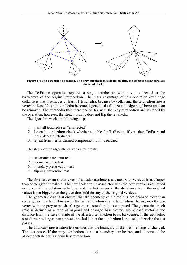
Libor Váša - Methods for dynamic mesh size reduction - State of the Art
- 36 -
Figure 17: The TetFusion operation. The prey tetrahedron is depicted blue, the affected tetrahedra are
depicted black.
The TetFusion operation replaces a single tetrahedron with a vertex located at the barycentre of the original tetrahedron. The main advantage of this operation over edge collapse is that it removes at least 11 tetrahedra, because by collapsing the terahedron into a vertex at least 10 other tetrahedra become degenerated (all face and edge neighbors) and can be removed. The tetrahedra that share one vertex with the prey tetrahedron are stretched by the operation, however, the stretch usually does not flip the tetrahedra.
The algorithm works in following steps: 1. mark all tetrahedra as “unaffected” 2. for each tetrahedron check whether suitable for TetFusion, if yes, then TetFuse and
mark affected tetrahedra 3. repeat from 1 until desired compression ratio is reached
The step 2 of the algorithm involves four tests: 1. scalar attribute error test 2. geometric error test 3. boundary preservation test 4. flipping prevention test
The first test ensures that error of a scalar attribute associated with vertices is not larger
than some given threshold. The new scalar value associated with the new vertex is computed using some interpolation technique, and the test passes if the difference from the original values is not bigger than the given threshold for any of the original vertices.
The geometric error test ensures that the geometry of the mesh is not changed more than some given threshold. For each affected tetrahedron (i.e. a tetrahedron sharing exactly one vertex with the prey tetrahedron) a geometric stretch ratio is computed. The geometric stretch ratio is defined as a ratio of original and changed base vector, where base vector is the distance from the base triangle of the affected tetrahedron to its barycentre. If the geometric stretch ratio is larger than a preset threshold, then the tetrahedron is refused, otherwise the test passes.
The boundary preservation test ensures that the boundary of the mesh remains unchanged. The test passes if the prey tetrahedron is not a boundary tetrahedron, and if none of the affected tetrahedra is a boundary tetrahedron.
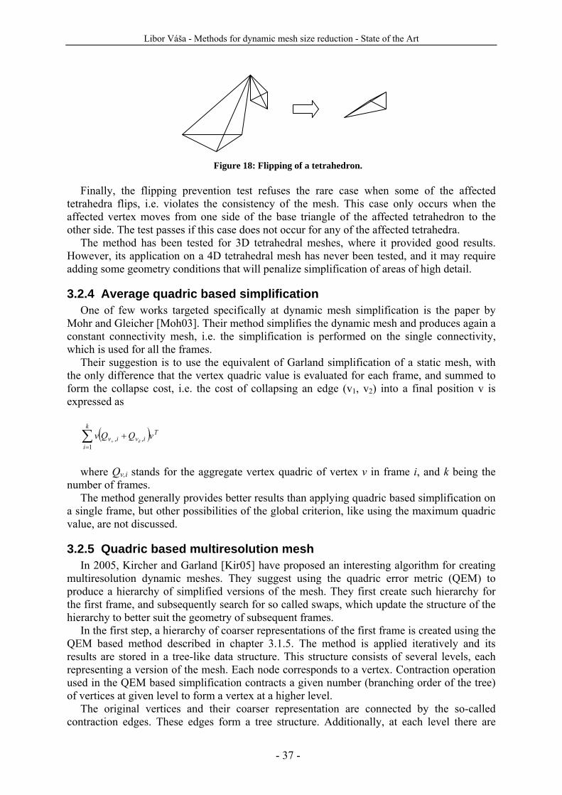
Libor Váša - Methods for dynamic mesh size reduction - State of the Art
- 37 -
Figure 18: Flipping of a tetrahedron.
Finally, the flipping prevention test refuses the rare case when some of the affected
tetrahedra flips, i.e. violates the consistency of the mesh. This case only occurs when the affected vertex moves from one side of the base triangle of the affected tetrahedron to the other side. The test passes if this case does not occur for any of the affected tetrahedra.
The method has been tested for 3D tetrahedral meshes, where it provided good results. However, its application on a 4D tetrahedral mesh has never been tested, and it may require adding some geometry conditions that will penalize simplification of areas of high detail.
3.2.4 Average quadric based simplification One of few works targeted specifically at dynamic mesh simplification is the paper by
Mohr and Gleicher [Moh03]. Their method simplifies the dynamic mesh and produces again a constant connectivity mesh, i.e. the simplification is performed on the single connectivity, which is used for all the frames.
Their suggestion is to use the equivalent of Garland simplification of a static mesh, with the only difference that the vertex quadric value is evaluated for each frame, and summed to form the collapse cost, i.e. the cost of collapsing an edge (v1, v2) into a final position v is expressed as
( )∑=
++
k
i
Tiviv vQQv
ě1
,,
where Qv,i stands for the aggregate vertex quadric of vertex v in frame i, and k being the
number of frames. The method generally provides better results than applying quadric based simplification on
a single frame, but other possibilities of the global criterion, like using the maximum quadric value, are not discussed.
3.2.5 Quadric based multiresolution mesh In 2005, Kircher and Garland [Kir05] have proposed an interesting algorithm for creating
multiresolution dynamic meshes. They suggest using the quadric error metric (QEM) to produce a hierarchy of simplified versions of the mesh. They first create such hierarchy for the first frame, and subsequently search for so called swaps, which update the structure of the hierarchy to better suit the geometry of subsequent frames.
In the first step, a hierarchy of coarser representations of the first frame is created using the QEM based method described in chapter 3.1.5. The method is applied iteratively and its results are stored in a tree-like data structure. This structure consists of several levels, each representing a version of the mesh. Each node corresponds to a vertex. Contraction operation used in the QEM based simplification contracts a given number (branching order of the tree) of vertices at given level to form a vertex at a higher level.
The original vertices and their coarser representation are connected by the so-called contraction edges. These edges form a tree structure. Additionally, at each level there are
Libor Váša - Methods for dynamic mesh size reduction - State of the Art
- 38 -
edges which represent the actual topology at the given level. These are actually necessary only for the finest level, but they are useful for updating the mesh during the reclustering of subsequent frames.
The multilevel mesh obtained by simplification of the first frame can be used for any other frame, however it may not be optimal, because the geometry of subsequent frames is different, and therefore the quadrics may also produce a higher error.
The key idea is to use the hierarchy from previous frame to the next frame, and to update it by moving vertices from one cluster to another. It is likely that only small changes are present in the mesh, and therefore only a small number of changes will take place. Therefore, instead of creating the whole structure for each frame from scratch, only a few so-called swaps are performed and encoded with the mesh.
A swap is a primitive operation of reclustering. As swap we denote moving a vertex v from cluster a to a cluster b. A swap is fully described by the (v,a,b) triplet, and in order to be performed at a given time, it has to be valid and beneficial. A set of such swaps is performed and encoded with each frame of the mesh, which ensures that the hierarchy well follows the geometry throughout the animation.
A swap is valid when following conditions are met: 1. there is a vertex in the cluster b, which shares a topology edge with v (i.e. v lies on the
border of a towards b. 2. v is not the only vertex in a 3. v is not a pinch vertex of a, i.e. when v is removed from a, a remains topologically
compact. A swap is beneficial, if the QEM is reduced. The benefit of the swap can be roughly
guessed as
( ) ( )aQbQb vv −= where Qv stands for the aggregate quadric of vertex v, and a and b are the positions of
vertices that correspond to the given two clusters at a coarser level of the mesh. This is a conservative guess, as the positions of a and b may change by the swap and therefore the benefit may be even higher.
However, it is necessary to ensure that not only the level immediately above the current level is positively influenced. Therefore, a generalized multilevel quadric metric is proposed, which sums the quadrics from all the levels with weights ensuring that the contributions from each level are uniform:
∑ ∑+= ∈
⎟⎟
⎠
⎞
⎜⎜
⎝
⎛=
n
ki Muui
i
EwE1
where Eu is the quadric error at vertex u of mesh level Mi. The weights wi are obtained as
follows:
β
⎟⎟⎠
⎞⎜⎜⎝
⎛=
=
++
i
iii M
Mww
w
11
0 1
Libor Váša - Methods for dynamic mesh size reduction - State of the Art
- 39 -
where |Mi| stands for the number of vertices at level i, and β is an empirically determined constant that compensates for the quadric value growth. The value of the constant has been determined to be 1.9127.
When the multilevel structure is created, it can be cut on any level, and only the original topology of that level, and its updates are then transmitted as the simplified version of the animation. This approach avoids the need of sending the complete topology with each frame, while it still allows altering the topology according to the changes in geometry.
We have identified two main drawbacks of this method. First, the method only uses temporally local information to determine the simplification. This may lead to a situation, when two subsequent frames are simplified in a radically different manner, and although both were originally similar and both were simplified locally optimally, they become very different. This behavior may occur repeatedly, resulting in some visible “flickering” artifacts.
The other drawback is that the number of vertices in each level of the representation remains constant throughout the span of the animation. The validity checks don’t allow disappearing of clusters, and there is no mechanism that would add new clusters when necessary.
Libor Váša - Methods for dynamic mesh size reduction - State of the Art
- 40 -
4 Evaluation tools There are two main approaches to evaluating the quality of data reduction. The first, based
on the concept of Peak Signal To Noise Ratio (PSNR) is used mainly in the field of compressions, where each vertex has its counterpart in the compressed representation of the mesh. This approach cannot be used in the case when the connectivity of the mesh is altered. In such case it is usual to evaluate some approximation of the Hausdorff distance between the meshes.
4.1.1 PSNR PSNR is a very simple measure of error mainly used to evaluate the accuracy of geometry
predictors. Its definition varies slightly with the used approaches, but usually takes following form:
( )
⎟⎟⎠
⎞⎜⎜⎝
⎛
∆−
= ∑=
N
i
ii
xxpredx
NPSNR
1
2)(1log20
Where N is the number of vertices predicted, x the actual position of each vertex, pred(x) is
the predicted position of the vertex, and x∆ is the span of values of the position, or the length of the body diagonal of the model.
The measure is easy to implement and fast to evaluate, but it has many drawbacks. First, it cannot be used when the connectivity of a mesh is changed. Second, it does not take into account that some movement causes larger disturbance in the mesh (movement orthogonal to the surface normal) while other may cause almost no disturbance at all (tangential movement).
4.1.2 Mesh, METRO One of the alternatives to PSNR is the Hausdorff distance. It is defined as a symmetric
maximal minimal distance between points of M and M’. It is usually not evaluated exactly, only some approximate value is found using some sampling algorithm ([Cig98], [Asp02]).
The Hausdorff distance definition starts with the one-way minimum distance from a point p to a mesh M:
( )MxpxMpd
∈−= min),(
where . represents the L2 norm. Note that not only vertices of M are used as x in the
previous equation, but also all the internal points of edges and faces of M. Now, we can define the one-way (forward) distance from mesh M to a mesh M’ as
( ) ( )( ) Mpf MpdMMd ∈′=′ ,max,
Again, all internal points of M are used as p in the previous equation. Finally, the
symmetric distance is defined as follows:
( ) ( ) ( )( ) ( )MMdMMdMMdMMd sffs ,',',',max', == This measure is usually not evaluated exactly, but some sampling technique is used. The
algorithms described in [Cig98] and [Asp02] sample both meshes uniformly, and then

Libor Váša - Methods for dynamic mesh size reduction - State of the Art
- 41 -
compute the maximum minimum distance between a set of points and a set of triangles using some spatial subdivision technique.
This measure can be applied “frame by frame” to a dynamic mesh, but it does not take into account the temporal properties of the dynamic mesh, i.e. the fact that some directions of the shift cause more disturbance because the mesh is evolving in orthogonal direction.
In section 5.1.1 we will describe a new tool for evaluating the difference between two
dynamic meshes, which overcomes the drawbacks of the methods presented here by combining the Hausdorff distance computation with 4D mesh representation.
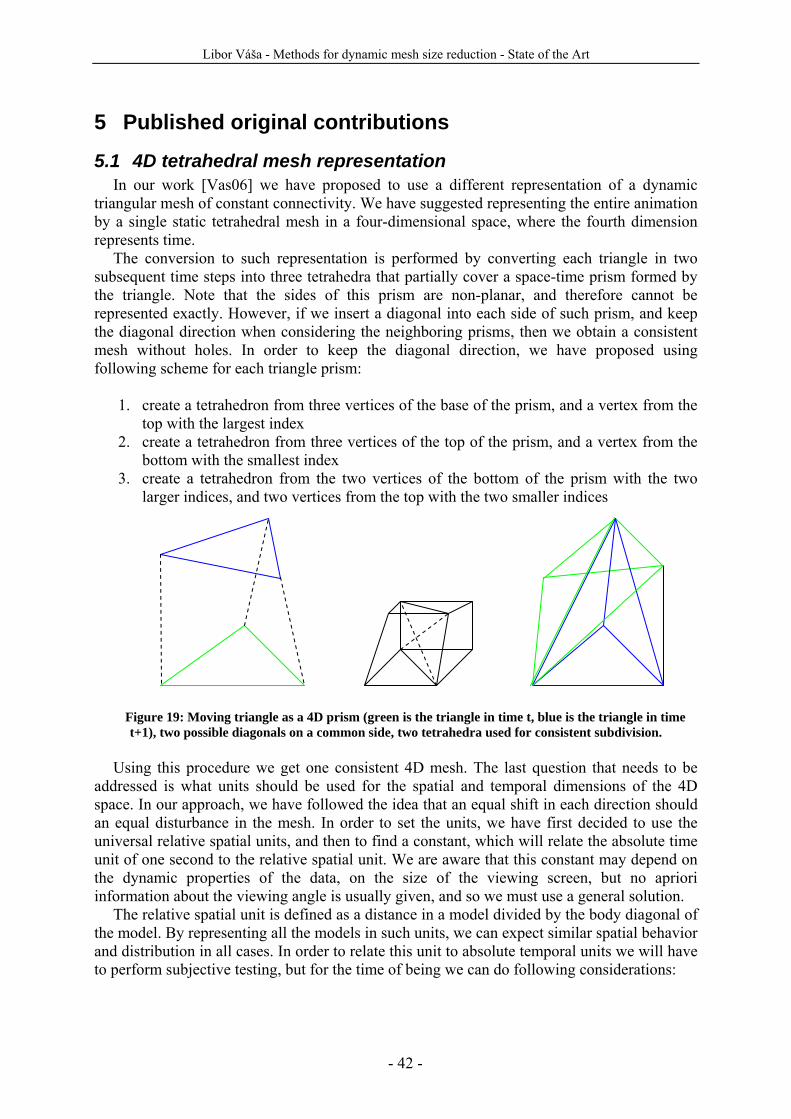
Libor Váša - Methods for dynamic mesh size reduction - State of the Art
- 42 -
5 Published original contributions
5.1 4D tetrahedral mesh representation In our work [Vas06] we have proposed to use a different representation of a dynamic
triangular mesh of constant connectivity. We have suggested representing the entire animation by a single static tetrahedral mesh in a four-dimensional space, where the fourth dimension represents time.
The conversion to such representation is performed by converting each triangle in two subsequent time steps into three tetrahedra that partially cover a space-time prism formed by the triangle. Note that the sides of this prism are non-planar, and therefore cannot be represented exactly. However, if we insert a diagonal into each side of such prism, and keep the diagonal direction when considering the neighboring prisms, then we obtain a consistent mesh without holes. In order to keep the diagonal direction, we have proposed using following scheme for each triangle prism:
1. create a tetrahedron from three vertices of the base of the prism, and a vertex from the
top with the largest index 2. create a tetrahedron from three vertices of the top of the prism, and a vertex from the
bottom with the smallest index 3. create a tetrahedron from the two vertices of the bottom of the prism with the two
larger indices, and two vertices from the top with the two smaller indices
Figure 19: Moving triangle as a 4D prism (green is the triangle in time t, blue is the triangle in time t+1), two possible diagonals on a common side, two tetrahedra used for consistent subdivision.
Using this procedure we get one consistent 4D mesh. The last question that needs to be
addressed is what units should be used for the spatial and temporal dimensions of the 4D space. In our approach, we have followed the idea that an equal shift in each direction should an equal disturbance in the mesh. In order to set the units, we have first decided to use the universal relative spatial units, and then to find a constant, which will relate the absolute time unit of one second to the relative spatial unit. We are aware that this constant may depend on the dynamic properties of the data, on the size of the viewing screen, but no apriori information about the viewing angle is usually given, and so we must use a general solution.
The relative spatial unit is defined as a distance in a model divided by the body diagonal of the model. By representing all the models in such units, we can expect similar spatial behavior and distribution in all cases. In order to relate this unit to absolute temporal units we will have to perform subjective testing, but for the time of being we can do following considerations:
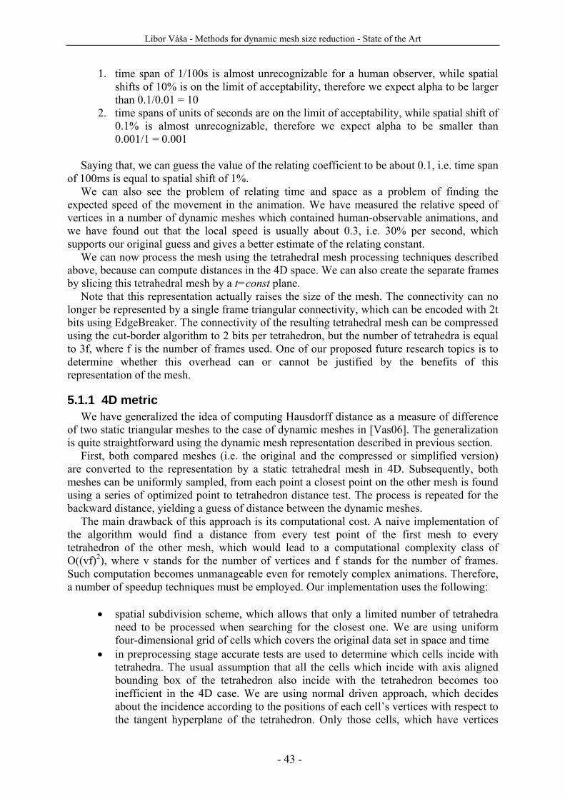
Libor Váša - Methods for dynamic mesh size reduction - State of the Art
- 43 -
1. time span of 1/100s is almost unrecognizable for a human observer, while spatial shifts of 10% is on the limit of acceptability, therefore we expect alpha to be larger than 0.1/0.01 = 10
2. time spans of units of seconds are on the limit of acceptability, while spatial shift of 0.1% is almost unrecognizable, therefore we expect alpha to be smaller than 0.001/1 = 0.001
Saying that, we can guess the value of the relating coefficient to be about 0.1, i.e. time span
of 100ms is equal to spatial shift of 1%. We can also see the problem of relating time and space as a problem of finding the
expected speed of the movement in the animation. We have measured the relative speed of vertices in a number of dynamic meshes which contained human-observable animations, and we have found out that the local speed is usually about 0.3, i.e. 30% per second, which supports our original guess and gives a better estimate of the relating constant.
We can now process the mesh using the tetrahedral mesh processing techniques described above, because can compute distances in the 4D space. We can also create the separate frames by slicing this tetrahedral mesh by a t=const plane.
Note that this representation actually raises the size of the mesh. The connectivity can no longer be represented by a single frame triangular connectivity, which can be encoded with 2t bits using EdgeBreaker. The connectivity of the resulting tetrahedral mesh can be compressed using the cut-border algorithm to 2 bits per tetrahedron, but the number of tetrahedra is equal to 3f, where f is the number of frames used. One of our proposed future research topics is to determine whether this overhead can or cannot be justified by the benefits of this representation of the mesh.
5.1.1 4D metric We have generalized the idea of computing Hausdorff distance as a measure of difference
of two static triangular meshes to the case of dynamic meshes in [Vas06]. The generalization is quite straightforward using the dynamic mesh representation described in previous section.
First, both compared meshes (i.e. the original and the compressed or simplified version) are converted to the representation by a static tetrahedral mesh in 4D. Subsequently, both meshes can be uniformly sampled, from each point a closest point on the other mesh is found using a series of optimized point to tetrahedron distance test. The process is repeated for the backward distance, yielding a guess of distance between the dynamic meshes.
The main drawback of this approach is its computational cost. A naive implementation of the algorithm would find a distance from every test point of the first mesh to every tetrahedron of the other mesh, which would lead to a computational complexity class of O((vf)2), where v stands for the number of vertices and f stands for the number of frames. Such computation becomes unmanageable even for remotely complex animations. Therefore, a number of speedup techniques must be employed. Our implementation uses the following:
• spatial subdivision scheme, which allows that only a limited number of tetrahedra
need to be processed when searching for the closest one. We are using uniform four-dimensional grid of cells which covers the original data set in space and time
• in preprocessing stage accurate tests are used to determine which cells incide with tetrahedra. The usual assumption that all the cells which incide with axis aligned bounding box of the tetrahedron also incide with the tetrahedron becomes too inefficient in the 4D case. We are using normal driven approach, which decides about the incidence according to the positions of each cell’s vertices with respect to the tangent hyperplane of the tetrahedron. Only those cells, which have vertices
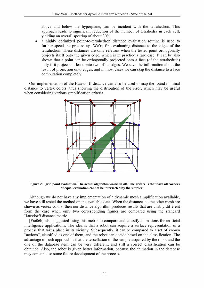
Libor Váša - Methods for dynamic mesh size reduction - State of the Art
- 44 -
above and below the hyperplane, can be incident with the tetrahedron. This approach leads to significant reduction of the number of tetrahedra in each cell, yielding an overall speedup of about 30%
• a highly optimized point-to-tetrahedron distance evaluation routine is used to further speed the process up. We’re first evaluating distance to the edges of the tetrahedron. These distances are only relevant when the tested point orthogonally projects itself onto the given edge, which is in practice a rare case. It can be also shown that a point can be orthogonally projected onto a face (of the tetrahedron) only if it projects at least onto two of its edges. We save the information about the result of projection onto edges, and in most cases we can skip the distance to a face computation completely.
Our implementation of the Hausdorff distance can also be used to map the found minimal
distance to vertex colors, thus showing the distribution of the error, which may be useful when considering various simplification criteria.
Figure 20: grid point evaluation. The actual algorithm works in 4D. The grid cells that have all corners
of equal evaluation cannot be intersected by the simplex. Although we do not have any implementation of a dynamic mesh simplification available,
we have still tested the method on the available data. When the distances to the other mesh are shown as vertex colors, then our distance algorithm produces results that are visibly different from the case when only two corresponding frames are compared using the standard Hausdorff distance metric.
[Fra06b] also suggested using this metric to compare and classify animations for artificial intelligence applications. The idea is that a robot can acquire a surface representation of a process that takes place in its vicinity. Subsequently, it can be compared to a set of known “actions”, classified as one of them, and the robot can decide based on the classification. The advantage of such approach is that the tessellation of the sample acquired by the robot and the one of the database item can be very different, and still a correct classification can be obtained. Also, the robot is given better information, because the animation in the database may contain also some future development of the process.
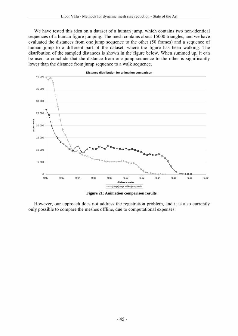
Libor Váša - Methods for dynamic mesh size reduction - State of the Art
- 45 -
We have tested this idea on a dataset of a human jump, which contains two non-identical sequences of a human figure jumping. The mesh contains about 15000 triangles, and we have evaluated the distances from one jump sequence to the other (50 frames) and a sequence of human jump to a different part of the dataset, where the figure has been walking. The distribution of the sampled distances is shown in the figure below. When summed up, it can be used to conclude that the distance from one jump sequence to the other is significantly lower than the distance from jump sequence to a walk sequence.
Distance distribution for animation comparison
0
5 000
10 000
15 000
20 000
25 000
30 000
35 000
40 000
0.00 0.02 0.04 0.06 0.08 0.10 0.12 0.14 0.16 0.18 0.20
distance value
occu
rren
ce
jump/jump jump/walk
Figure 21: Animation comparison results. However, our approach does not address the registration problem, and it is also currently
only possible to compare the meshes offline, due to computational expenses.
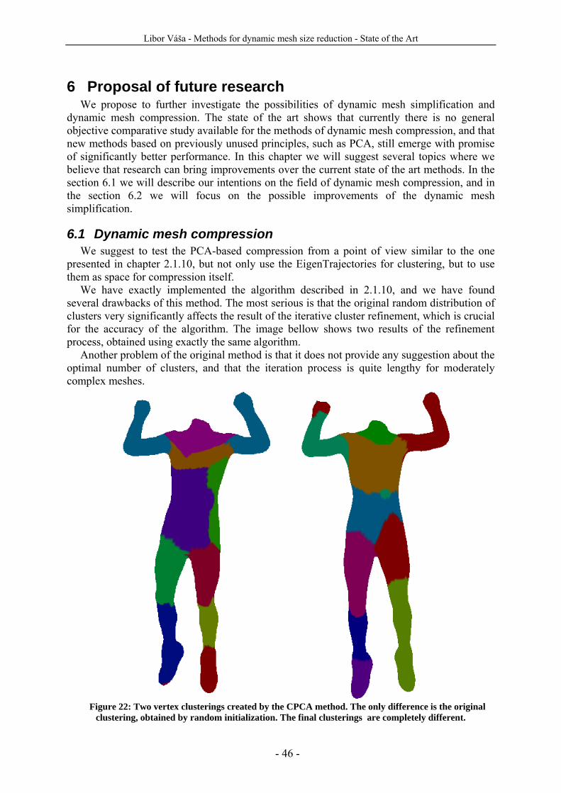
Libor Váša - Methods for dynamic mesh size reduction - State of the Art
- 46 -
6 Proposal of future research We propose to further investigate the possibilities of dynamic mesh simplification and
dynamic mesh compression. The state of the art shows that currently there is no general objective comparative study available for the methods of dynamic mesh compression, and that new methods based on previously unused principles, such as PCA, still emerge with promise of significantly better performance. In this chapter we will suggest several topics where we believe that research can bring improvements over the current state of the art methods. In the section 6.1 we will describe our intentions on the field of dynamic mesh compression, and in the section 6.2 we will focus on the possible improvements of the dynamic mesh simplification.
6.1 Dynamic mesh compression We suggest to test the PCA-based compression from a point of view similar to the one
presented in chapter 2.1.10, but not only use the EigenTrajectories for clustering, but to use them as space for compression itself.
We have exactly implemented the algorithm described in 2.1.10, and we have found several drawbacks of this method. The most serious is that the original random distribution of clusters very significantly affects the result of the iterative cluster refinement, which is crucial for the accuracy of the algorithm. The image bellow shows two results of the refinement process, obtained using exactly the same algorithm.
Another problem of the original method is that it does not provide any suggestion about the optimal number of clusters, and that the iteration process is quite lengthy for moderately complex meshes.
Figure 22: Two vertex clusterings created by the CPCA method. The only difference is the original
clustering, obtained by random initialization. The final clusterings are completely different.
Libor Váša - Methods for dynamic mesh size reduction - State of the Art
- 47 -
We suggest creating a new PCA-based compression scheme using following
improvements:
• Subtract the position of the first vertex from each trajectory. This simple step partially removes the geometry coherence of the original data, and yields a set of trajectories, where each starts in the origin. Note that this step has significantly different effect from subtracting the cluster centers suggested by [Sat05], which has basically no effect at all, because subsequently the mean of the PCA input is subtracted as a first step of PCA. We have found that subtracting the first vertex position improves the results of the PCA, however further experiments with different datasets will be needed in order to get an objective measure about the amount of accuracy gain.
• Replace the random initialization of the cluster centers by some heuristic, which may also provide some suggestion about the number of clusters needed. One such heuristic could be the PCA itself, applied in the first step on all the trajectories. The initial clustering can be derived from the indices of n largest PCA coefficients of each vector. The advantage of such approach is that for simple animations, such as translation motions, it will correctly suggest a single cluster, because only one principal trajectory will have the largest coefficient for all the trajectories in the data set. However, our experiments so far show that this approach sometimes suggests too many clusters, some of which have only a very few members, and therefore we may need some cluster merging algorithm or a completely different initial heuristic.
• For cases when only a small number of clusters is suggested by the estimator we suggest to perform a single PCA over all the trajectories, compare its results to the clustered case and use the better one according to the rate/distortion ratio. Our implementation of the EigenTrajectory based PCA already outperforms the original spatial PCA method by Alexa [Ale00] (see figure 24), while it is easier to implement, because it does not require the rigid motion removal step. It is also significantly faster (the example in figure 24 has been computed about order of magnitude faster), because it performs eigenvalues decomposition over a covariance matrix of size 3f x 3f, while the original method required a singular value decomposition of a 3v x f matrix, and usually the number of frames is much lower than the number of vertices
Another problem, that we have identified in most of the compression algorithms, is that
they usually only aim to minimize the overall MSE value. We suggest using some different error metric, such as the one proposed in chapter 5.1.3 instead. The most straightforward application is using this metric in the quantization step.
Quantizers usually offer several positions of the vertex, which can be encoded with given number of bits, and they choose the one that is closest to the original point position. However, it is possible that this position is sub-optimal with respect to the Hausdorff distance error introduced by the quantization. Using our metric it may be possible to improve the similarity of the original and encoded versions of the animations, although the MSE may become larger.
Unfortunately, such approach cannot be applied for the case of PCA based methods, and at current stage we don’t know about any way how to combine a more rigorous error metric with PCA based compressors.
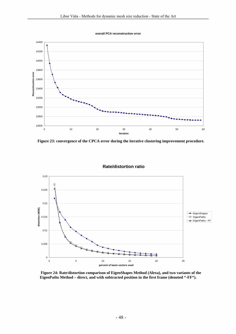
Libor Váša - Methods for dynamic mesh size reduction - State of the Art
- 48 -
overall PCA reconstruction error
12600
12800
13000
13200
13400
13600
13800
14000
14200
14400
0 10 20 30 40 50 60
Iteration
Rec
osnt
ruct
ion
erro
r
Figure 23: convergence of the CPCA error during the iterative clustering improvement procedure.
Rate/distortion ratio
0
0.005
0.01
0.015
0.02
0.025
0.03
0 5 10 15 20 25
percent of basis vectors used
dist
ortio
n (M
SE)
EigenShapesEigenPathsEigenPaths - FF
Figure 24: Rate/distortion comparison of EigenShapes Method (Alexa), and two variants of the EigenPaths Method – direct, and with subtracted position in the first frame (denoted “-FF“).
Libor Váša - Methods for dynamic mesh size reduction - State of the Art
- 49 -
6.2 Dynamic mesh simplification As for the area of dynamic mesh simplification, the state of the art presented above shows
that there has been only a very limited amount of work published in this area, and basically only two papers specifically address this problem. Dynamic mesh simplification will receive increasing importance in the following years, and we suggest focusing our research into this area.
There are two main issues that distinguish the dynamic case of simplification from the well studied static problem. First, the dynamic properties of the data can (and should) be exploited, i.e. the similarity of subsequent meshes should be used to obtain better compression ratios. Most of the methods presented in the state of the art do exploit the dynamic properties of the data.
Second, the dynamicity of the problem should be addressed, i.e. considered when looking for some optimal solution. In other words, optimal solutions in separate frames are not necessarily optimal as a solution for the whole sequence, and information about simplification of temporally neighboring frames should be taken into account during the simplification.
We suggest four possible scenarios: Frame by frame simplification, spatio-temporal simplification of a 4D representation of the mesh, single connectivity simplification using global simplification criteria and multiresolution approach similar to the one described in chapter 3.2.5. We suggest using our spatio-temporal Hausdorff distance evaluation tool to find the best possible way to simplify a dynamic mesh.
6.2.1 Frame by frame simplification The first possibility we’re suggesting is simplifying each frame independently. This
approach leads to meshes of varying connectivity, which exploit the spatial coherence of separate time steps. The expected compressed size of the connectivity is 2tf bits for t triangles in f frames. Any existing simplification techniques can be used, and therefore the method can be steered to any compression ratio, however the temporal coherence of the mesh remains unused, and neither can it be used for geometry prediction, because the topology of subsequent frames is different, and therefore the correspondence of vertices of subsequent frames is lost.
We’re only mentioning this approach to cover the full range of possibilities; we don’t expect it to be very efficient. The method does not exploit nor does it address dynamicity of the mesh.
6.2.2 Spatio-temporal simplification The second approach is the spatio-temporal scheme, where the 4D static tetrahedral mesh
representation is simplified using some tetrahedral mesh simplification technique. Both spatial and temporal coherence can be exploited, and can be used in both simplification and geometry prediction.
The final mesh sequence will need to be extracted from the simplified tetrahedral representation by cutting it by a plane of t=const., which represents the mesh state at given time. We will need to explore the possibilities of performing this slicing on the GPU, as it will be performed by the decoder in real-time.
From the accuracy point of view, the crucial choice is the selection of the simplification criterion. The possibilities that we would like to implement and test are the following:
• The quadric based simplification. Its n-dimensional extension can be directly
applied on the 4D tetrahedral mesh representation, however the method requires to store a quadric with each vertex, which may lead to unacceptable memory
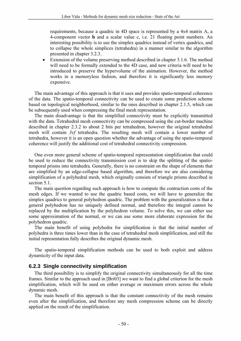
Libor Váša - Methods for dynamic mesh size reduction - State of the Art
- 50 -
requirements, because a quadric in 4D space is represented by a 4x4 matrix A, a 4-component vector b and a scalar value c, i.e. 21 floating point numbers. An interesting possibility is to use the simplex quadrics instead of vertex quadrics, and to collapse the whole simplices (tetrahedra) in a manner similar to the algorithm presented in chapter 3.2.3.
• Extension of the volume preserving method described in chapter 3.1.6. The method will need to be formally extended to the 4D case, and new criteria will need to be introduced to preserve the hypervolume of the animation. However, the method works in a memoryless fashion, and therefore it is significantly less memory expensive.
The main advantage of this approach is that it uses and provides spatio-temporal coherence
of the data. The spatio-temporal connectivity can be used to create some prediction scheme based on topological neighborhood, similar to the ones described in chapter 2.1.5, which can be subsequently used when compressing the final mesh representation.
The main disadvantage is that the simplified connectivity must be explicitly transmitted with the data. Tetrahedral mesh connectivity can be compressed using the cut-border machine described in chapter 2.3.2 to about 2 bits per tetrahedron, however the original tetrahedral mesh will contain 3vf tetrahedra. The resulting mesh will contain a lower number of tetrahedra, however it is an open question whether the advantage of using the spatio-temporal coherence will justify the additional cost of tetrahedral connectivity compression.
One even more general scheme of spatio-temporal representation simplification that could
be used to reduce the connectivity transmission cost is to skip the splitting of the spatio-temporal prisms into tetrahedra. Generally, there is no constraint on the shape of elements that are simplified by an edge-collapse based algorithm, and therefore we are also considering simplification of a polyhedral mesh, which originally consists of triangle prisms described in section 5.1.
The main question regarding such approach is how to compute the contraction costs of the mesh edges. If we wanted to use the quadric based costs, we will have to generalize the simplex quadrics to general polyhedron quadric. The problem with the generalization is that a general polyhedron has no uniquely defined normal, and therefore the integral cannot be replaced by the multiplication by the polyhedron volume. To solve this, we can either use some approximation of the normal, or we can use some more elaborate expression for the polyhedron quadric.
The main benefit of using polyhedra for simplification is that the initial number of polyhedra is three times lower than in the case of tetrahedral mesh simplification, and still the initial representation fully describes the original dynamic mesh.
The spatio-temporal simplification methods can be used to both exploit and address
dynamicity of the input data.
6.2.3 Single connectivity simplification The third possibility is to simplify the original connectivity simultaneously for all the time
frames. Similar to the approach used in [Bri03] we want to find a global criterion for the mesh simplification, which will be used on either average or maximum errors across the whole dynamic mesh.
The main benefit of this approach is that the constant connectivity of the mesh remains even after the simplification, and therefore any mesh compression scheme can be directly applied on the result of the simplification.
Libor Váša - Methods for dynamic mesh size reduction - State of the Art
- 51 -
The main drawback is that the efficiency of the global simplification criteria is likely to be dependent on the nature of the dynamic mesh. We expect that animations of bodies that do not significantly change their shape in time will compress well using this method. However, radical changes of shape, such as growth of new features, or complete shape morphing, will probably lead to oversampling of some areas in some frames, thus yielding sub-optimal simplification.
Single connectivity based methods only exploit dynamicity of the input in a limited way, and also the dynamicity-caused problems are only addressable partially.
6.2.4 Multiresolution approach The multiresolution approach described in chapter 3.2.5 provides a very elegant alternative
to the three methods described so far in this chapter. It allows different topology in subsequent frames, while it does not require the complete topology of each frame to be transmitted, using the fact that the topologies are likely to be similar, and therefore only the changes in topology between frames are sent to the decoder.
We have identified that the main drawback of this method is that it basically only uses spatial simplification criterion. In each frame, only the vertices of the given time instant are used to determine which edges should be collapsed. This way it is possible, that for subsequent frames of the mesh two different simplified versions are used, both being optimal from the point of view of the frame, although very different one from the other, which may cause some visible artifacts (shaking of the surface). In other words, the method does not address the problems of dynamicity of the data.
We suggest fixing this problem by using the spatio-temporal representation of the mesh to determine the collapse costs. Each edge collapse in the multiresolution representation corresponds to an edge collapse in the spatio-temporal representation (however not the other way round!), and therefore we can keep both the representations at the same time and use one for encoding (multiresolution), and the other for determining the collapse costs (4D tetrahedral mesh).
A more radical augmentation of the multiresolution method would be introducing tree
optimization steps that would allow adding and removing new clusters according to changes in geometry of the mesh. The removal of clusters can be added trivially by removing the validity constraint that disallows vertex swap when a vertex is the only member of its cluster.
However, addition of clusters may prove to be more difficult. We suggest adding a “cluster split” operation that will be performed on clusters that have too big overall quadric value. Although finding a constant threshold that would determine the clusters for splitting may be difficult or even impossible, using a relative difference to average quadric values of other clusters may provide a robust solution.
Augmenting the multiresolution approach in this way will lead to non-constant number of clusters at each level, which will require additional operations to be encoded with the changes in the topology. Subsequent compression techniques will also need to be slightly modified, however for example modification of a predictor encoders is quite straightforward, the only difference is that some vertices will not have a successor in following frames, and some vertices will share predecessors from the previous frame.
Libor Váša - Methods for dynamic mesh size reduction - State of the Art
- 52 -
The proposed approaches are summarized in the following table:
Method Coherency exploiting Connectivity cost Usable predictors
Frame by frame Spatial only 2tf Spatial only
Spatio-temporal Spatial and temporal 6tf Spatio-temporal tetrahedral predictors
Single connectivity Spatial and temporal 2t Spatio-temporal
Multiresolution Spatial for simplification (to be augmented to spatio-temporal),
temporal for connectivity 2t+updates Modified spatio-temporal
One of the methods that will most likely be used in all of the three approaches is the
quadric based simplification. We would also like to test this method using different approaches to constructing the aggregate quadrics. This intention is inspired by the various vertex normal estimation schemes ([Max99], [Thu98]), where weighting by simplex area usually isn’t the best possibility.
Generally, the current scheme is equivalent to computing the vertex quadric as sum of incident simplex quadrics weighted by the area (volume, hypervolume etc.) of the corresponding simplices. We suggest trying different schemes, namely:
• weighting by relative incident angle, i.e. simplices with large incident angle will
have larger impact on the vertex quadric. • weighting by inverse area/volume. Although this may seem contra-intuitive, it can
be actually mathematically justified ([Max99]). In fact, the smaller the simplex, the more it tells about the behavior of the shape in the vicinity of the vertex, and therefore the bigger impact it should have on the vertex quadric.
• weighting by combination of the previous weights, especially the angle/area weight proposed by [Max99] could provide improvement of the results obtained by quadric based simplification methods.
To summarize the future research goals, we propose focusing our efforts on the following
topics: • evaluation of the proposed PCA based compression with various initial heuristics • evaluation of the compression schemes minimizing Hausdroff distance instead of
MSE • design and verification of the multiresolution scheme for dynamic meshes and its
evaluation with collapse costs obtained from 4D representation • augmentation the multiresolution approach by adding the cluster removal/split
operations • design and verification of 4D mesh simplification algorithms based on
o edge collapse/vertex quadrics o tetfusion/simplex quadrics o edge collapse/polyhedral quadrics
• performance evaluation of the 4D mesh simplification schemes above The final result of the proposed doctoral thesis will ideally be a compatible combination of
an efficient simplification algorithm and an efficient compression algorithm, which will allow encoding dynamic meshes with wide range of compression ratios, and which will both address and exploit the dynamicity of the input data.
Libor Váša - Methods for dynamic mesh size reduction - State of the Art
- 53 -
References [Ale00] Alexa M., Müller W.: Representing animations by principal components. Computer Graphics
Forum, 19(3), pages 411-418, 2000. [Alg96] Algorri M.E., Schmitt F.: Mesh simplification. In Proceedings of Eurographics ’96, pages 78-86,
1996. [All02] Alliez P., Gotsman C.: Recent Advances in Compression of 3D Meshes. In "Advances in
Multiresolution for Geometric Modelling", N.A. Dodgson, M.S. Floater, M.A. Sabin (Eds.), Springer, 2004.
[All05] Alliez P., Ucelli G., Gotsman C., Attene M.: Recent Advances in Remeshing of Surfaces. Springer, 2005.
[Asp02] Aspert N., Santa-Cruz D., Ebrahimi T.: Mesh: Measuring errors between surfaces using the Hausdorff distance. In Proceedings of the IEEE International Conference on Multimedia and Expo, volume I, pages 705-708, 2002.
[Att03] Attene M., Falcidieno B., Spagnuolo M., Rossignac J.: SwingWrapper: Retiling triangle meshes for better EdgeBreaker compression, ACM Transactions on Graphics, 22(4), 2003.
[Ben05] Ben-Chen M., Gotsman C.: On the Optimality of Spectral Compression of Mesh Data. ACM Transactions on Graphics, 24(1):60-80, 2005.
[Bri03] Briceno H.M., Sander P.V., McMillan L., Gortler S., Hoppe H.: Geometry Videos: A new representation for 3D Animations. In Proceedings of ACM Symposium on Computer Animation 2003, 2003.
[Cal98] Calderbank A., Daubechies I., Sweldens W., Yeo B.: Wavelet transforms that map integers to integrers. Applied and Computational Harmonic Analysis, vol. 5, no. 3, pages 332-369, 1998.
[Cam98] Campagna S., Kobbelt L., Seidel H.-P.: Efficient Decimation of Complex Triangle Meshes. Technical Report 3, Computer Graphics Group, University of Erlangen, Germany, 1998.
[Cam99] Campagna S., Kobbelt L., Schneider R., Seidel H.-P., Vorsatz J.: Mesh Reduction and Interactive Multiresolution Modeling on Arbitrary Triangle Meshes. In Proceedings SCCG, 1999.
[Cig98] Cignoni P., Rocchini C., Scopigno R.: Metro: Measuring Error on Simplified Surfaces. Computer Graphics Forum 17, 2, pages 167-174, 1998.
[Cig98] Cignoni P., Rocchini C., Scopigno R.: Metro: Measuring Error on Simplified Surfaces. Computer Graphics Forum 17, 2, pages 167-174, 1998.
[Coo99] Coors V., Rossignac J.: Delphi: geometry-based connectivity prediction in triangle mesh compression. Vis. Comput. 20, 8-9 (Nov. 2004), pages 507-520, 2004.
[Čer02] Čermák M., Skala V.: Polygonization by the Edge Spinning. 16th Conference on Scientific Computing, Algoritmy 2002, Slovakia, ISBN 80-227-1750-9, pages 8-13, 2002.
[Flo97] Floater M.: Parametrization and smooth approximation of surface triangulations. CAGD 14, 3, pages 231-250, 1997.
[Fra01] Franc M., Skala V.: Parallel Triangular Mesh Decimation Without Sorting. In SCCG 2001 Conference Proceedings, Comenius University Bratislava, Slovakia, ISBN 80-223-1606-7, pages 69-75, 2001.
[Fra02] Franc M.: Methods for Polygonal Mesh Simplification. Technical Report No. DCSE/TR-2002-01, University of West Bohemia, 2002.
[Fre00] Frey P.J.: About surface remeshing. In Proceedings of the 9th International Meshing Roundtable, pages 123-136, 2000.
[Gar05] Garland M., Zhou Y.: Quadric-based simplification in any dimension. ACM Transactions on Graphics, Volume 24 , Issue 2, Pages: 209-239, 2005
[Gar97] Garland M., Heckbert P.S.: Surface simplification using quadric error metrics. Proceedings of the 24th annual conference on Computer graphics and interactive techniques, pages 209-216, 1997.
[Got02] Gotsman C., Gumhold S., Kobbelt L.: Simplification and Compression of 3D Meshes. In "Tutorials on Multiresolution in Geometric Modelling", A. Iske, E. Quak, M.S. Floater (Eds.), Springer, 2002.
[Gu02] Gu X., Gortler S., Hoppe H.: Geometry Images. In Proc. 29th SIGGRAPH, pages 355-361, San Antonio, TX, 2002.
[Gum98] Gumhold S., Straßer W.: Real time compression of triangle mesh connectivity. SIGGRAPH '98, pages 133-140, 1998.
[Gum99] Gumhold S., Guthe S., Straßer W.: Tetrahedral Mesh Compression with the Cut-Border Machine. In Proceedings of the 10th Annual IEEE Visualization Conference, 1999.
[Hir99] Hirota G., Maheshvari R., Lin M.C.: Fast volume-preserving free form deformation using multi-level optimization. Proceedings of the fifth ACM symposium on Solid modeling and applications, Ann Arbor, Michigan, United States, pages: 234-245, 1999.
Libor Váša - Methods for dynamic mesh size reduction - State of the Art
- 54 -
[Hop96] Hoppe H.: ACM SIGGRAPH 1996, pages 99-108, 1996 [Cho02] Chopra P., Meyer J.: TetFusion: An Algorithm For Rapid Tetrahedral Mesh Simplification. In
Proc. IEEE Visualization, pages 133-140, 2002. [Iba03] Ibarria L., Rossignac J.: Dynapack: space-time compression of the 3D animations of triangle
meshes with fixed connectivity. Proceedings of the 2003 ACM SIGGRAPH/Eurographics symposium on Computer animation, San Diego, California, 2003.
[Kar00] Karni Z., Gotsman C.: Spectral Compression of Mesh Geometry. Computer Graphics (Proceedings of SIGGRAPH), pages 279-286, 2000.
[Kar04] Karni Z., Gotsman C.: Efficient Compression of Soft-Body Animation Sequences. Computers and Graphics, 28:25-34, 2004.
[Kir05] Kircher S., Garland M.: Progressive Multiresolution Meshes for Deforming Surfaces. ACM/Eurographics Symposium on Computer Animation, pages 191-200, 2005.
[Kro02] Kronrod B., Gotsman C.: Optimized Compression of Triangle Mesh Geometry Using Prediction Trees. Proceedings of the International Symposium on 3D Data Processing, Visualization and Transmission, Padua, 2002.
[Lin98] Lindstrom P., Turk G.: Fast and memory efficient polygonal simplification. Proceedings of the conference on Visualization '98, Research Triangle Park, North Carolina, United States, pages 279-286, 1998.
[Lin99] Lindstrom P., Turk G.: Evaluation of Memoryless Simplification. In IEEE Transactions on Visualization and Computer Graphics, 5(2), 1999.
[Mar03] Marpe D., Wiegand T., Schwarz H.: Context-based adaptive binary arithmetic coding in the H.264/AVC video compression standard. IEEE Trans. Circuits Syst. Video Techn. 13(7), pages 620-636, 2003.
[Max99] Max N: Weights for Computing Vertex Normals from Facet Normals. Journal of Graphics Tools, 4(2), pages 1-6, 1999.
[Moh03] Mohr A., Gleicher M.: Deformation sensitive decimation. Tech. Rep. 4/7/2003, University of Wisconsin, Madison, 2003.
[Mul05] Müller K., Smolic A., Kautzner M., Eisert P., Wiegand T.: Predictive Compression of Dynamic 3D Meshes. Proc. ICIP2005, IEEE International Conference on Image Processing, Genoa, Italy, 2005.
[Mul07] Müller K., Smolic A., Kautzner M., Eisert P., Wiegand T.: Rate-Distortion-Optimized Predictive Compression of Dynamic 3D Mesh Sequences. Signal Processing: Image Communication, EURASIP Journal, 2007.
[Pay05] Payan F., Antonini M.: Wavelet-based Compression of 3D Mesh Sequences. Proceedings of IEEE 2nd ACIDCA-ICMI'2005, Tozeur, Tunisia, 2005.
[Pop97] Popovic J., Hoppe H.: Progressive simplicial complexes. ACM SIGGRAPH 1997, pages 217-224, 1997.
[Ron96] Ronfard R., Rossignac J.: Full range approximation of triangulated polyhedra. In Proceedings of Eurographics ’96, pages 67-76, 1996.
[Ros99] Rossignac J.: Edgebreaker: Connectivity compression for triangle meshes. IEEE Transactions on Visualization and Computer Graphics, Vol. 5, No. 1, 1999.
[San02] Sander P., Gortler S., Snyder J., Hoppe H.: Signal-Specialized Parametrization. Microsoft Research MSR-TR-2002-27, 2002.
[Sat05] Sattler M., Sarlette R., Klein R.: Simple and efficient compression of animation sequences. Proceedings of the 2005 ACM SIGGRAPH/Eurographics symposium on Computer animation (SCA 2005), pages 209-217, 2005.
[Sez02] Sezer C.: Simplification of Tetrahedral Meshes by Scalar Value Assignment. MSc. Thesis at Bilkent University, 2002.
[Sha01] Shamir A., Pascucci V., Temporal and Spatial Level of Details for Dynamic Meshes. Proceedings of Virtual Reality Systems and Techniques, pages 423-430, 2001.
[Sch92] Schroeder W.J., Zarge J.A., Lorensen W. E.: Decimation of Triangle Meshes, Computer Graphics (SIGGRAPH '92 Proceedings), Vol. 26, No. 2, pages 65-70, 1992
[Sta98] Staadt O.G., Gross M.H.: Progressive Tetrahedralizations. In Proceedings of IEEE Visualization '98, pages 397-402, 1998.
[Ste06] Stefanoski N., Ostermann J.: Connectivity-Guided Predictive Compression of Dynamic 3D Meshes. International Conference on Image Processing (ICIP), 2006.
[Sur05] Surazhsky V., Gotsman C.: A Qualitative Comparison of Some Mesh Simplification Software Packages. Preprint, Mar 2005.
[Szy99] Szymczak A., Rossignac J.: Grow&Fold: compression of tetrahedral meshes. Technical Report GIT-GVU-99-02, Georgia Institute of Technology, 1999.
Libor Váša - Methods for dynamic mesh size reduction - State of the Art
- 55 -
[Tau98] Taubin G., Rossignac J.: Geometric compression through topological surgery. ACM Transactions on Graphics, Volume 17 , Issue 2, Pages: 84-115. 1998.
[Thu98] Thurmer G., Wuthrich C.A.: Computing vertex normals from polygonal facets. J. Graph. Tools 3, 1, pages 43-46, 1998.
[Tou98] Touma C., Gotsman C.: Triangle Mesh Compression. Proceedings of Graphics Interface, Vancouver, June 1998.
[Yan02] Yang J., Kim C., Lee S.-U.: Compression of 3D triangle mesh sequences based on vertex-wise motion vector prediction, IEEE Trans. Circuits Syst. Video Technol., vol. 12, no. 12, pages 1178-1184, 2002.
[Zha04] Zhang J., Owen C.B.: Octree-based Animated Geometry Compression. DCC '04, Data Compression Conference, Snowbird, Utah, USA, pages 508-517, 2004.
Publications [Vas06] Váša L., Skala V.: A Spatio-Temporal Metric for Dynamic Mesh Comparison. In proceedings of
AMDO2006 Int.conf, Spain, Springer-Verlag LNCS 4069, pages 29-37, 2006. [Fra06a] Frank M., Váša L., Skala V.: MVE-2 Applied in Education Process. Proceedings of .NET
Technologies 2006, Pilsen, Czech Republic, 2006. [Fra06b] Frank M., Váša L., Skala V.: Pipeline approach used for recognition of dynamic meshes.
Proceedings of 3IA 2006, Limoges, France, 2006. [Vas05a] Váša, L.; Hanák, I.; Skala, V.: Improved Super-Resolution Method and Its Acceleration,
Proceedings of EUSIPCO 2005, 2005. [Vas05b] Váša, L.; Skala, V.: Resolution Improvement of Digitized Images, Proceedings of Algoritmy 2005 [Vas04] Váša, L.: Resolution Improvement of Digitized Images, Diploma thesis at University of West
Bohemia, 2004.

Libor Váša - Methods for dynamic mesh size reduction - State of the Art
- 56 -
Appendix A – Project assignments, other activities 2003 – normal vector computation approaches – comparative study 2005 – present: MVE2 project leader, development of a modular visualization environment 2005 – present: 3DTV project 2006 – present: CPG LC Centre, core member
Stays abroad Sept. 2003 – Feb. 2004 – Erasmus/Socrates stay at University of Bath, United Kingdom 2004 – ECI ‘2004, Herlany, Slovakia 2005 – Algoritmy 2005, Podbanske, Slovakia 2005 – EUSIPCO, Antalya, Turkey Feb. 2006 – May 2006 – internship at First Numerics Inc., Cardiff, United Kingdom 2006 – 3IA, Limoges, France 2006 – AMDO 2006, Mallorca, Spain
Teaching activities 2004/2005:
• Foundations of Computer Graphics (KIV/ZPG) – tutorials • Programming for .NET (KIV/NET) – lectures, tutorials • Basics of .NET and C# - lecture for ZPG students
2005/2006: • Foundations of Computer Graphics (KIV/ZPG) – tutorials • Digital photography – lecture • Introduction to Quantum computing – lecture • Basics of .NET and C# - lecture for ZPG students