Embed Size (px)
Citation preview
Methods and Simulation Tools for Cavity Design
Prof. Dr. Ursula van Rienen, Dr. Hans-Walter Glock
SRF09 Berlin - Dresden
Dresden 18.9.09

U. van Rienen, H.-W. Glock2
Overview
• Introduction
• Methods in Computational Electromagnetics (CEM)
• Examples of CEM Methods:
• Finite Integration Technique (FIT)
• Coupled S-Parameter Simulation (CSC)
• Simulation Tools
• Practical Examples
• Some generalities
• Some selected examples

U. van Rienen, H.-W. Glock3
Overview
• Introduction
• Methods in Computational Electromagnetics (CEM)
• Examples of CEM Methods:
• Finite Integration Technique (FIT)
• Coupled S-Parameter Simulation (CSC)
• Simulation Tools
• Practical Examples
• Some generalities
• Some selected examples

U. van Rienen, H.-W. Glock4
Superconducting accelerator cavities
www.kek.jp/intra-e/press/2005/image/ilc1.jpg [Podl], IAP Frankfurt/M.
Jefferson Lab / http://www.physics.umd.edu/courses/Phys263/Kelly/cavity.jpg
http://www.linearcollider.org/newsline/images/2008/20080501_dc_1.jpg
http://irfu.cea.fr/Images/astImg/2407_2.jpg
... and some other types
=> Often chains of repeated structures, combined with flanges / coupling devices.

U. van Rienen, H.-W. Glock5
I) Accelerating Mode:• Do match?
• How much energy does the particle gain?
• How much energy is stored in the cavity?
• How big is the power loss in the wall? And how big is the unloaded quality factor?
• Where are the maxima of electric (field emission) and magnetic (quench) field strength at the surface? Which values do they reach?
What do you need to know?
Jefferson Lab
2 20 0
2 2ε μ
= =∫∫∫ ∫∫∫cav cav
amplitude amplitudestoredV V
W E dV H dV
ΔEkin = qpart Ez (z) ⋅ cos(2π fres z / vpart +ϕ0 ) dzz=0
z=Lcav
∫
2 2tan tan 0
1 ;2 2 2
ω μ ωσ
= = ⋅ =∫∫ ∫∫surface res res storedloss
losscavity cavity
R WP H dA H dA QP
( )2 and part res cellv f L

U. van Rienen, H.-W. Glock6
What do you need to know?II) Fundamental passband:• All resonant frequencies! Which frequency spread does the fundamental passband have? How close is the next neighbouring mode to the accelerating mode? Cell-to-Cell coupling filling time
• How strong is the beam interaction of all modes?Look at “R over Q”:
III) Higher Order Modes (HOM):• same questions as for fundamental passband• wake potential kick factor• special field profiles strongly confined far away from couplers: "trapped modes"
RQ=
ΔEkin
qpart
⎛
⎝⎜⎞
⎠⎟
2
ω resWstored( )
fmode/MHz
cell-to-cell phase advance ϕ

U. van Rienen, H.-W. Glock7
What do you need to know?
IV) Input and HOM-coupler/absorber:• Qloaded of all beam-relevant modes
• Field distortions due to coupler?
• Field distribution within the coupler
V) Multipacting
VI) Mechanical stability wrt. Lorentz Forces
CAD-plot: DESY

U. van Rienen, H.-W. Glock8
What do you need to know?
Jefferson Lab
I) Accelerating modeII) Fundamental passbandIII) HOMsIV) Input and HOM-coupler/absorberV) Multipacting
VI) Mechanical stability wrt. Lorentz Forces
Eigenmodes provide most of the information needed:
100% of I)100% of II)80% of III)25% of IV)25% of V)50% of VI)

U. van Rienen, H.-W. Glock9
Overview
• Introduction
• Methods in Computational Electromagnetics (CEM)
• Examples of CEM Methods:
• Mode Matching Technique
• Finite Integration Technique (FIT)
• Coupled S-Parameter Simulation (CSC)
• Simulation Tools
• Practical Examples
• Some generalities
• Some selected examples

U. van Rienen, H.-W. Glock10
Need for Numerical Methods
Most practical electrodynamics problems cannot be solved purely by means of analytical methods, see e.g.:
• radiation caused by a mobile phone near a human head
• shielding of an electronic circuit by a slotted metallic box
• mode computation in accelerator cavities, especially in chains of cavities
In many of such cases, numerical methods can be applied in an efficient way to come to a satisfactory solution.

U. van Rienen,
Numerical Methods
Semi-analytical Methods• Methods based on Integral Equations• Method of Moments (MoM)
Discretization Methods• Finite Difference Method (FD)• Boundary Element Method (BEM)• Finite Element Method (FEM)• Finite Volume Method (FVM)• Finite Integration Technique (FIT)
Possible Problems• Need for geometrical simplifications MoM• Violation of continuity conditions FD• Unfavorable matrix structures BEM• Unphysical solutions FEM if not mixed FEM• Etc.

U. van Rienen, H.-W. Glock12
Discretization (I) of Solution itself
Picture source:http://www.integra.co.jp/eng/whitepapers/inspirer/inspirer.htm
Discretization error; 1D and 2D

U. van Rienen, H.-W. Glock13
Discretization (II) of Boundary of Solution Domain
Picture source:http://www.sri.com/poulter/crash/crown_victoria/crvic_figures/fig_cvic2.html
Structured „boundary-fitted“ grid
In general: geometrical error

U. van Rienen, H.-W. Glock14
Discretization (III) – Spatial Grid Types
Picture source:http://www.uni-karlsruhe.de/RZ/Dienste/GVM/DIENSTE/CAE-ANWENDUNGEN/FIDAP/erfahrung/node46.html
Unstructured 2D grid:

U. van Rienen,
Discretization (V) – Space and Time
3 +
space time grid space grid time
G T
⊗ → ×
⊗ → ×R R
Laptop withWLAN card
4,96 A/m=H
=0,085 A/mH
2,4 GHzf = Computed with CST MWS

U. van Rienen, H.-W. Glock16
Grid Time Example
Wave propagation in rectangular waveguide
Energy density of „wake fields“ in the TESLA cavity

U. van Rienen, H.-W. Glock17
Overview
• Introduction
• Methods in Computational Electromagnetics (CEM)
• Examples of CEM Methods:
• Finite Integration Technique (FIT)
• Coupled S-Parameter Simulation (CSC)
• Simulation Tools
• Practical Examples
• Some generalities
• Some selected examples

U. van Rienen, H.-W. Glock18
FIT Grid

U. van Rienen,
i j k l nbe et
e e ∂+ − − = −
∂
.. . .1 . 1 . 1 . 1
.
.
.. .. .
i
j
k
l
n
e
be
te
e
⎛ ⎞⎜ ⎟⎜ ⎟
⎛ ⎞⎜ ⎟⎛ ⎞ ⎜ ⎟∂⎜ ⎟⎜ ⎟− − =− ⎜ ⎟⎜ ⎟⎜ ⎟ ∂ ⎜ ⎟⎜ ⎟ ⎜ ⎟ ⎜ ⎟⎝ ⎠ ⎝ ⎠⎜ ⎟⎜ ⎟⎜ ⎟⎝ ⎠e
bC
=̂
FIT Discretization of Induction Law
t∂
= −∂
Ce bA A
E ds B dAt∂
∂⋅ = − ⋅
∂∫ ∫∫
nb
ieje
ke
le

U. van Rienen,
0i j k l m nb b b b b b+ + − − − =
. .. 1 1 1 1 1 1
.
.
.
..
i
j
k
l
m
n
b
b
b
b
b
b
⎛ ⎞⎜ ⎟⎜ ⎟⎜ ⎟⎜ ⎟⎜ ⎟⎛ ⎞⎜ ⎟⎜ ⎟− − − =⎜ ⎟⎜ ⎟
⎜ ⎟ ⎜ ⎟⎝ ⎠ ⎜ ⎟⎜ ⎟⎜ ⎟⎜ ⎟⎜ ⎟⎜ ⎟⎝ ⎠
0
S
b
=̂ =Sb 00V
d∂
⋅ =∫∫ B A
jb
ib nb
kblbmb
FIT Discretization of Gauss Law
U. van Rienen,
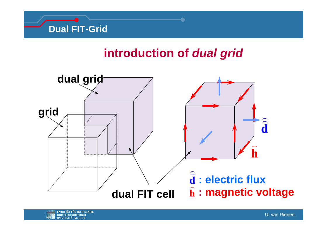
introduction of dual grid
dual grid
dual FIT cell
Dual FIT-Grid
gridd
h
: electric flux: magnetic voltageh
d

U. van Rienen,
FIT equations on the dual grid
A A
d dt∂
∂⎛ ⎞⋅ = + ⋅⎜ ⎟∂⎝ ⎠∫ ∫∫DH s J A
V V
d dV∂
ρ⋅ = ⋅∫∫ ∫∫∫D A
t∂∂
= +Ch d j
=Sd q d
h
FIT Discretization of Ampère‘s and Coulomb‘s Law

U. van Rienen,
curl
curl
divdiv 0
ρ
∂= −
∂∂
= +∂
==
t
t
BE
DH J
DB
FIT
t
t
∂= −
∂∂
= +∂
=
=
Ce b
Ch d j
Sd q
Sb 0
=
=
= +
ε
μ
κ e
d M e
b M h
j M e je
εμκ
=== +
D EB HJ E J
Maxwell‘s „Grid Equations“ (MGE)
T. Weiland, 1977, 1985

U. van Rienen, H.-W. Glock24
Shape Approximation on Cartesian Grids
ModellingCurved Boundaries
Staircase FDTD/FDFD(standard) : poor convergence
Conformal FIT / PBA: 2nd order convergencealways applicableKrietenstein, Schuhmann, Thoma,Weiland 1998
FIT withnon-equidistant step size:2nd order convergencenot always applicableWeiland 1977
FIT with diagonal filling:better convergenceWeiland 1977
FIT on non-orthogonal grids2nd order accuracy
R.Schuhmann, 1998

U. van Rienen,
FIT on Triangular Grids
U. van Rienen 1983
Grid Dual grid
URMEL-T

U. van Rienen, H.-W. Glock26
FIT on Non-Orthogonal Grids
Hilgner, Schuhmann, WeilandTU Darmstadt 1998
TESLA 9 cell struct. (Grid representation, N=13x69x13=11.661)
Field in model of 1 cell

U. van Rienen,
curl
curl
divdiv 0
ρ
∂= −
∂∂
= +∂
==
t
t
BE
DH J
DB
FIT
t
t
∂= −
∂∂
= +∂
=
=
Ce b
Ch d j
Sd q
Sb 0
=
=
= +
ε
μ
κ e
d M e
b M h
j M e je
εμκ
=== +
D EB HJ E J
Maxwell‘s „Grid Equations“ (MGE) Curl Curl Equation
T. Weiland, 1977, 1985
In full analogy toanalytical derivation of wave equation

U. van Rienen, H.-W. Glock28
Curl-Curl-Eigenvalue Equation
( )( )no current excitation
0, , real loss-freeS
µσ ε
≡
=
j 0
11 2
µε ω−− =M CM C e e
eigenvalue problem
λ=Ax x
11CC µε
−−=A M CM C
1 -1 2curl curlµε ω− =E E

U. van Rienen, H.-W. Glock29
Curl-Curl-Eigenvalue Equation
1/2Use transformation ' to derive an equation with symmetric system matrix
ε=e M e
11/2 1/2 2' '
µε ε ω−− =M CM CM e e
( )( )
1/2 1/2
1/2 1/21
1/2 1/2 1/2 1/2
system matrix '
is symmetric
CC
µ
T
µ µ
ε ε
ε ε
ε ε
−
− −−
− − − −
=
=
=
A M A M
M CM CM
M CM M CM
U. van Rienen, H.-W. Glock30
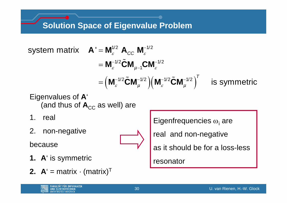
Solution Space of Eigenvalue Problem
( )( )
1/2 1/2
1/2 1/21
1/2 1/2 1/2 1/2
system matrix '
is symmetric
CC
µ
T
µ µ
ε ε
ε ε
ε ε
−
− −−
− − − −
=
=
=
A M A M
M CM CM
M CM M CM
Eigenvalues of A‘(and thus of ACC as well) are
1. real
2. non-negative
because
1. A‘ is symmetric
2. A‘ = matrix · (matrix)T
Eigenfrequencies ωi are
real and non-negative
as it should be for a loss-less
resonator

U. van Rienen, H.-W. Glock31
Overview
• Introduction
• Methods in Computational Electromagnetics (CEM)
• Examples of CEM Methods:
• Finite Integration Technique (FIT)
• Coupled S-Parameter Simulation (CSC)
• Simulation Tools
• Practical Examples
• Some generalities
• Some selected examples

U. van Rienen, H.-W. Glock32
Coupled S-Parameter Calculation
Coupled S-Parameter Calculation
H.-W. Glock, K.Rothemund, UvR 98

U. van Rienen, H.-W. Glock33
Overview
• Introduction
• Methods in Computational Electromagnetics (CEM)
• Examples of CEM Methods:
• Finite Integration Technique (FIT)
• Coupled S-Parameter Simulation (CSC)
• Simulation Tools – not exhaustive
• Practical Examples
• Some generalities
• Some selected examples

U. van Rienen, H.-W. Glock34
CST STUDIO Suite
CST MICROWAVE STUDIO®
-Transient Solver
- Eigenmode Solver
- Frequency Domain Solver
- Resonant: S-Parameters and Fields
- Integral Equations Solver
- Predecessors for eigenmode calculation: MAFIA, URMEL, URMEL-T
http://www.cst.com/

U. van Rienen, H.-W. Glock35
HFSS
http://www.ansoft.com/products/hf/hfss/

U. van Rienen, H.-W. Glock36
ACE3P Suite
https://confluence.slac.stanford.edu/display/AdvComp/Omega3P
ACE3P - Advanced Computational Electromagnetic Simulation Suitedeveloped at SLAC by the group around Kwok Ko, Cho NG et al.
See examples in next part of the talk

U. van Rienen, H.-W. Glock37
Overview
• Introduction
• Methods in Computational Electromagnetics (CEM)
• Examples of CEM Methods:
• Mode Matching Technique
• Finite Integration Technique (FIT)
• Coupled S-Parameter Simulation (CSC)
• Simulation Tools
• Practical Examples
• Some generalities
• Some selected examples

U. van Rienen, H.-W. Glock38
Workflow of eigenmode computation
define geometry / import CAD-data
take care of your grid
define material properties
define symmetries and boundaries
check solver parameters
run solver (and maybe: wait)
frequency range ok ???
precision ok ???
(quasi) mode degeneration ???
post process: visualization
post process: derived quantities

U. van Rienen, H.-W. Glock39
Workflow of eigenmode computation
define symmetries and boundaries

U. van Rienen, H.-W. Glock40
Passband Fields with Etan = 0 in middle of the cavity
TM010- π/5 (pseudo 0) TM010-3π/5 TM010-π (accelerating)
Monopole-type E- and H-field, common to all modes and cells
Make use of symmetry compute only ½ of the cavity
Computed withCST MWS

U. van Rienen, H.-W. Glock41
Passband Fields with Htan = 0 in middle of the cavity
TM010-2π/5 TM010-4π/5
Use of symmetrycompute only
½ of thecavity
Needs of course 2
(shorter) runs!
Visualizationof full cavityprovided byCST MWS
Even 1/8 partmight be
enough forcomputation Computed with
CST MWS

U. van Rienen, H.-W. Glock42
Passband Fields altogether
TM010-2π/5
TM010-4π/5
TM010-π
TM010-3π/5
TM010-π/5700.40098 MHz
702.21446 MHz
704.52333 MHz
706.34471 MHz
706.97466 MHz
fmode/MHz
cell-to-cell phase advance ϕ
... which seems to obey some rule ?!
Computed withCST MWS
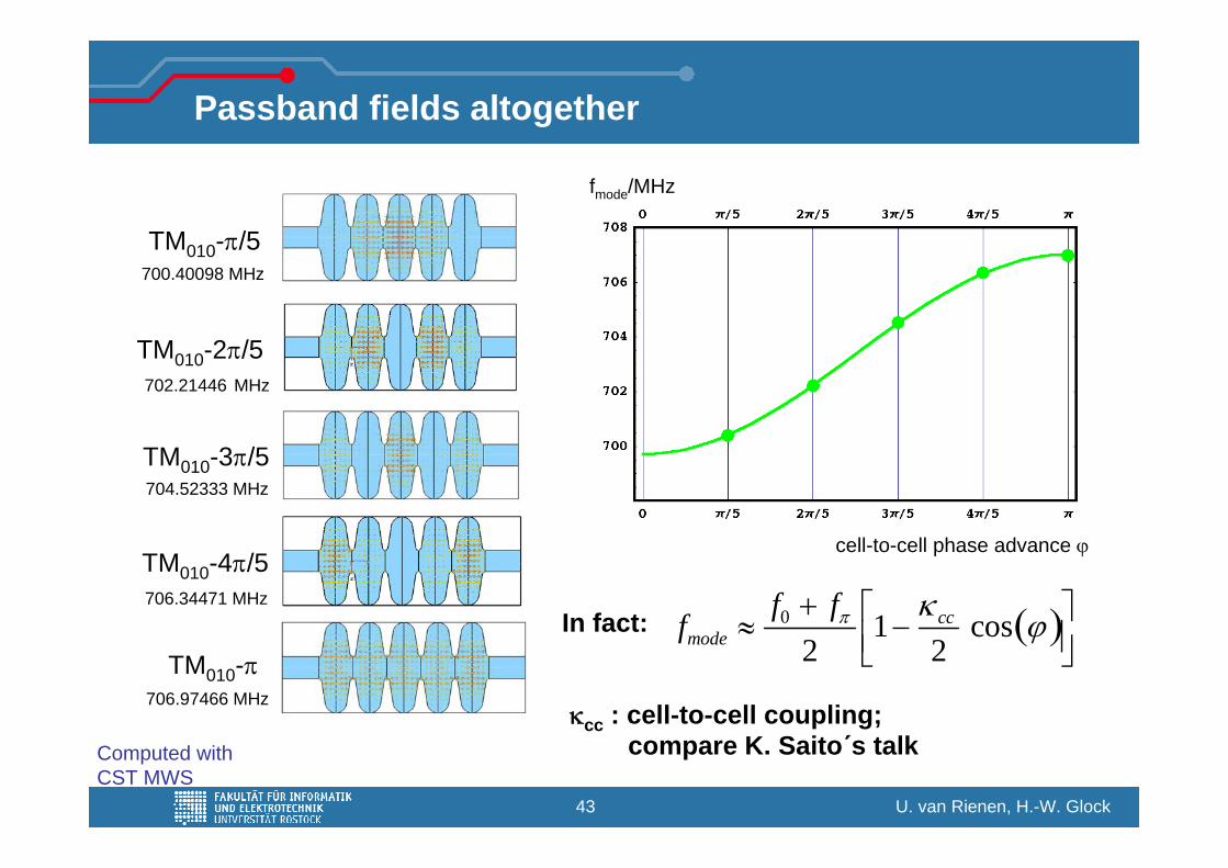
U. van Rienen, H.-W. Glock43
Passband fields altogether
TM010-2π/5
TM010-4π/5
TM010-π
TM010-3π/5
TM010-π/5700.40098 MHz
702.21446 MHz
704.52333 MHz
706.34471 MHz
706.97466 MHz
fmode/MHz
cell-to-cell phase advance ϕ
In fact:
κcc : cell-to-cell coupling; compare K. Saito´s talk
fmode ≈f0 + fπ
21−
κ cc
2cos ϕ( )⎡
⎣⎢⎤⎦⎥
Computed withCST MWS

U. van Rienen, H.-W. Glock44
So, what are passbands?
fmode/MHz
cell-to-cell phase advance ϕ
Cavities built by chains of identical cells show resonances in certainfrequency intervalls, called passbands, determined only by the shape of the elementary cell. The distribution of resonances in the band depends on the number of cells in the chain:
5-cell-chainresonances
12-cell-chainresonances
Computed withCST MWS
U. van Rienen, H.-W. Glock45
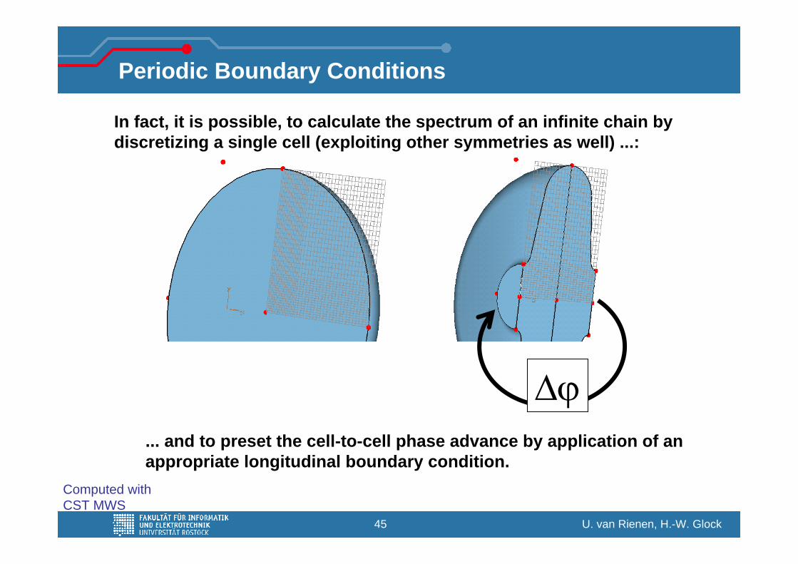
Periodic Boundary Conditions
In fact, it is possible, to calculate the spectrum of an infinite chain bydiscretizing a single cell (exploiting other symmetries as well) ...:
... and to preset the cell-to-cell phase advance by application of an appropriate longitudinal boundary condition.
Δϕ
Computed withCST MWS

U. van Rienen, H.-W. Glock46
fmode/MHz
cell-to-cell phase advance ϕ
Periodic Boundary Conditions
This needs only one single run for each Δϕ, but gives eigenmodefrequencies of several passbands with a very small grid (here 19,000 mp), e.g:
Computed withCST MWS

U. van Rienen, H.-W. Glock47
What are Monopole-, Dipole-, Quadrupole-Modes?Consider structures of axial circular symmetry. Then all fields belongto classes with invariance to certain azimuthal rotations:
Monopole, any ϕ Dipole, ϕ =180°
Quadrupole, ϕ =90°
Sextupole, ϕ =60°
Oktupole, ϕ =45°
Dekapole, ϕ =36°Computed withCST MWS

U. van Rienen, H.-W. Glock48
Trapped Mode Analysis
Search for strongly confined field distributions by simulating samestructure with different waveguide terminations at beam pipe ends. Compare spectra! Small frequency shifts indicate weak coupling.
E_18: 2039.66 MHzH_19: 2040.81 MHz
E_17: 2037.1373 MHzH_18: 2037.1746 MHzE t
an=
0
Hta
n=
0
Hta
n=
0
E tan
= 0
Remark: TE11-cut off of beam pipe at 1953 MHzComputed withCST MWS

U. van Rienen, H.-W. Glock49
Overview
• Introduction
• Methods in Computational Electromagnetics (CEM)
• Examples of CEM Methods:
• Mode Matching Technique
• Finite Integration Technique (FIT)
• Coupled S-Parameter Simulation (CSC)
• Simulation Tools
• Practical Examples
• Some generalities
• Some selected examples

U. van Rienen, H.-W. Glock50
TESLA 9-Cell Structure
Niobium; acceleration at 1.3 GHz
Field on axis
z/m
E z(n
orm
iert
)
Foto: DESY
2D-simulation of upper half; only azimuthal symmetry exploitedComputed withMAFIA

U. van Rienen, H.-W. Glock51
Filling of TESLA “Superstructure“- Semi-analytical calculation
„Superstructure“, J. Sekutowicz 1997
λ / 2
Structure of CDR
3 λ / 29 λ / 2 7 λ / 2
H.-W. Glock; D. Hecht; U. van Rienen; M. Dohlus. Filling and Beam Loading in TESLA Superstructures. Proc. of the 6th European Particle Accelerator Conference EPAC98, (1998): 1248-1250.
0 1 2 3 4
t = T2500200015001000500
0 z/m
Ez /(V/m)
0
Ez /(kV/m)
0 1 2 3 4
t = 1000 T
z/m
100200300
-300-200-100
Ez /(MV/m)
0 1 2 3 4
t = 106 T
z/m
02040
-40-20
rf period T = 0.7688517112 ns
Computed with MAFIA

U. van Rienen, H.-W. Glock52
Dipole mode 28, f = 2. 574621 GHz
317 VAs/m10041.1 −⋅ 312 VAs/m10196.2 −⋅
Dipole mode 29, f = 2. 584735 GHz
319 VAs/m10272.1 −⋅ 312 VAs/m10662.2 −⋅
Dipole mode 30, f = 2. 585019 GHz
318 VAs/m10109.9 −⋅ 312 VAs/m10578.2 −⋅
Higher Order Modes in TESLA Structure
Computed withMAFIA

U. van Rienen, H.-W. Glock53
CSC - 9-Cell Resonator with Couplers
• Resonator without couplers: N ~ 29,000 (2D)N ~ 12·106 (3D)
• Resonator with couplers: N ~ 15·106 (3D)⇒ N increases by ~ 500
• CSC: „Coupled S-Parameter Calculation“ allows forcombination of 2D- and 3D-simulations
HOMcoupler
HOMcoupler
Input coupler
CAD-plot: DESY
K. Rothemund; H.-W. Glock; U. van Rienen. Eigenmode Calculation of Complex RF-Structures using S-Parameters. IEEE Transactions on Magnetics, Vol. 36, (2000): 1501-1503.

U. van Rienen, H.-W. Glock54
CSC - Resonator Chain – Variation of Tube Length
Identical sectionsHOM1
HOM2
Variation ofcoupler position1,000 frequency points31 lengthsresulting S-matrix: 16 x 16 intern 84 x 84,1h 12min, Pentium III, 1 GHz
⏐SH
om1H
om2 ⏐/
dB
Weak dependence on position Computed with MAFIA, CST MWS and our own Mathematica Code for CSC

U. van Rienen, H.-W. Glock55
Effect of Changed Coupler Design*
R=-1 R=-1
L1 L1L2,u L2,d
L1 = 45.0 mmL2,u = 101.4 mmL2,d = 65.4 mm
S-parameters of TESLA cavity: Modal analysis**
S-parameters of HOM- & HOM-input-coupler:CST MicrowaveStudio®
CSC to determine S-parameters of various object combinations
*New concept: M. Dohlus, DESY; ** Modal coeff. computed by M. Dohlus H.-W. Glock, K. Rothemund

U. van Rienen, H.-W. Glock56
2,5 GHz 2,54 GHz 2,58 GHz2,46 GHz
107
105
104
106
Q
Comparison: HOM(original) – HOM(mirrowed)
HOM (up)
HOM (down)
mirrowed
2,5 GHz 2,54 GHz 2,58 GHz2,46 GHz
107
105
104
106
Q
In cooperation with M. Dohlus, DESY
H.W. Glock; K. Rothemund; D. Hecht; U. van Rienen. S-Parameter-Based Computation in Complex Accelerator Structures: Q-Values and Field Orientation of Dipole Modes. Proc. ICAP 2002
Computed with MAFIA, CST MWS and our own Mathematica Code for CSC

U. van Rienen, H.-W. Glock57
Some of his slides …Courtesy to Martin Dohlus

U. van Rienen, H.-W. Glock58
Courtesy of M. Dohlus, DESY – ICAP 2009

U. van Rienen, H.-W. Glock59
Courtesy of M. Dohlus, DESY – ICAP 2009

U. van Rienen, H.-W. Glock60
Courtesy of M. Dohlus, DESY – ICAP 2009

U. van Rienen, H.-W. Glock61
Courtesy of M. Dohlus, DESY – ICAP 2009

U. van Rienen, H.-W. Glock62
Courtesy of M. Dohlus, DESY – ICAP 2009

U. van Rienen, H.-W. Glock63
Courtesy of M. Dohlus, DESY – ICAP 2009

U. van Rienen, H.-W. Glock64
Courtesy of M. Dohlus, DESY – ICAP 2009

U. van Rienen, H.-W. Glock65
Courtesy of Cho Ng, Lixin Ge

U. van Rienen, H.-W. Glock66
CLIC HDX Simulation
Fields enhanced around slot rounding
E
Es/Ea=2.80Es/Ea=2.26
Hs/Ea=0.0044 A/m/(V/m)Hs/Ea=0.0049
A/m/(V/m)
Hs/Ea=0.0040 A/m/(V/m)
H
HDX Surface E & B Fields
Courtesy of Cho Ng, Lixin Ge

U. van Rienen, H.-W. Glock67
Electron Trajectory & Impact Energy
Particles emitted from one of the irisesAt 85 MV/m gradient, energy of dark current electrons can reach ~0.4 MeV on impact
emitted here
Courtesy of Cho Ng, Lixin Ge

U. van Rienen, H.-W. Glock68
At the end ....
... some other "cavity" type. Hope, you feel better.
Wilhelm Busch: Max und Moritz, sometimes in the 19th century. Widely publishedhttp://upload.wikimedia.org/wikipedia/commons/thumb/c/c2/Max_und_Moritz_(Busch)_026.png/800px-Max_und_Moritz_(Busch)_026.png
These are greetings of my co-author Hans-Walter Glock ….