Embed Size (px)
Citation preview
DEPwmßswTOF warn* snwmmmsm STÜÄFORO.CAUFÖ««
10DS AND APPLICATIONS OF TIME SERIES ANALYSIS PART II: LINEAR STOCHASTIC MODELS
TECHNICAL REPORT NO. 12
T. W. ANDERSON AND N. D. SINGPURWALLA
OCTOBER 1984
U. S. ARMY RESEARCH OFFICE CONTRACT DAAG29-82-K-1056
THEODORE W. ANDERSON, PROJECT DIRECTOR
DEPARTMENT OF STATISTICS STANFORD UNIVERSITY STANFORD, CALIFORNIA
*1Ä 3 1 tt
APPROVED FOR PUBLIC RELEASE; DISTRIBUTION UNLIMITED.

METHODS AND APPLICATIONS OF TIME SERIES ANALYSIS
PART II: LINEAR STOCHASTIC MODELS
TECHNICAL REPORT NO. 12
T. W. ANDERSON STANFORD UNIVERSITY
and
N. D. SINGPURWALLA* THE GEORGE WASHINGTON UNIVERSITY
OCTOBER 1984
U. S. ARMY RESEARCH OFFICE
CONTRACT DAAG29-82-K-0156
Also issued as GWU/IRRA/T-84/11, The Institute for Reliability and Risk Analysis, School of Engineering and Applied Science,
George Washington University, Washington D.C. 20052.
Research Supported by Grant DAAG29-84-K-0160, U.S. Army Research Office, and Contract N00014-77-C-0263, Project NR042-372, Office of Naval Research, with The George Washington University.
DEPARTMENT OF STATISTICS STANFORD UNIVERSITY STANFORD, CALIFORNIA
APPROVED FOR PUBLIC RELEASE; DISTRIBUTION UNLIMITED.

THE VIEW, OPINIONS, AND/OR FINDINGS CONTAINED IN THIS REPORT ARE THOSE OF THE AUTHOR(S) AND SHOULD NOT BE CONSTRUED AS AN OFFICIAL DEPARTMENT OF THE ARMY POSITION, POLICY, OR DECISION, UNLESS SO DESIGNATED BY OTHER DOCUMEN- TATION.

CONTENTS
Methods and Applications of Time Series Analysis
Part II: Linear Stochastic Models
5. Introduction to Autoregressive Models 1
5.1 Stationary Stochastic Processes 2
5.1.1. Examples of Stationary Stochastic Processes 6
6. Basic Notions of Multivariate Normal Distributions 9
7. Estimation of the Correlation Function 12
8. Autoregressive Processes 16
8.1 Representation as an Infinite Moving Average 17
8.1.1. Conditions for Convergence in the Mean of Auto- regressive Processes 20
8.2 Evaluation of the Coefficients 6 and their Behavior 24
8.2.1. Special Cases Describing the Evaluation and the Behavior of <5 's 26
8.3 The Covariance Function of an Autoregressive Process 32
8.3.1. Special Cases Describing the Behavior of the Autocovariance Function of an Autoregressive Process 34
8.3.2. Behavior of the Estimated Autocorrelation Function of Some Simulated Autoregressive Processes 41
8.4 Expressing the Parameters of an Autoregressive Process in Terms of Autocorrelations 49
8.5 The Partial Autocorrelation Function of an Autoregressive Process 50
8.5ol. Relationship between Partial Autocorrelation and the Last Coefficient of an Autoregressive Process 53
8.5.2, Behavior of the Estimated Partial Autocorrelation Function of Some Simulated Autoregressive Processes 56
8.6 An Explanation of the Fluctuations in Autoregressive Processes 64
8.7 Autoregressive Processes with Independent Variables 65
8.8 Stationary Autoregressive Processes Whose Associated Polynomial Equation Have at Least One Root Equal to 1 69
8.9 Some Linear Nonstationary Processes 71
8.9.1. Behavior of the Covariance Function of 73 Integrated Autoregressive Processes
8.9.2. The Covariance Function of Some Processes with an Underlying Trend 77
8.9.3. Behavior of Estimated Autocorrelation Function of a Real Life Nonstationary Time Series 86
8.10 Forecasting (Prediction) for Stationary Autoregressive Processes 93
8.11 Examples of Some Real Life Time Series Described by Autoregressive Processes 96
8.11.1. The Weekly Rotary Rigs in Use Data 96
8.11.2. The Landsat 2 Satellite Data 107
n
-1-
5. Introduction to Autoregressive Models
In the previous sections we considered models for time series in
which the characteristic and useful properties appropriate to the time
sequence were embodied in the mean function f(t) ; f(t) could be a
polynomial or a trigonometric function. In astronomy, for example, it
is reasonable to suppose that the effect of time is mainly in f(t)
and thus prediction is reasonable. In economics and weather, for
example, the random part u, is also time dependent, and thus predic-
tion is more difficult. When the effect of time is embodied in u. ,
we are led to a "stochastic process" whose characteristic properties
are described by the underlying probabilistic structure. In these
cases, for example, there are not regular periodic cycles but more or
less irregular fluctuations that have statistical properties of varia-
bility. A process whose probability structure does not change with
time is called stationary. In Section 5 we are mainly interested in
processes that are stationary or almost stationary or such that at
least the probability aspect (as distinguished from a deterministic
mean value function) is roughly stationary.
To illustrate these ideas, let us consider an autoregressive
process of order one, which is described by the relationship
yt = pyt-l + ut ' t = 1>2"-- »
where the y 's are observed values of a random variable, and the u 's
are some unobserved random variables, called innovations. The innovation
ut is assumed independent of y. , »y+p" • • f°r a^ values of t.

•2-
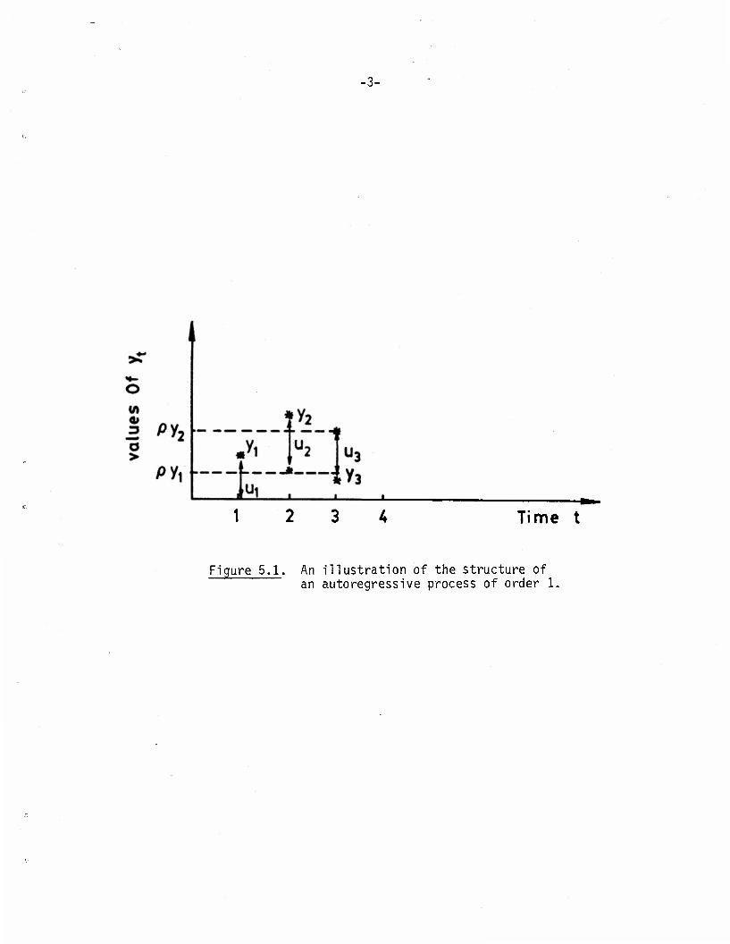
The distribution of y, and y2 is given by the distribution of
y, and py.+u^, and similarly the distribution of y,, y2, and y3
is given by the distribution of y,, py-, + u2 , and p(py.+u2)+u3 .
Thus y- depends on y2 , which in turn depends upon y« , and so on.
If |p| <1 , then the further apart the y's, the less they are related.
An innovation u? is absorbed into y,, y»,..., and thus the randomness
perpetuates in time. We therefore say that the effect of time is
embodied in the u.'s . The above process is pictorially described in
Figure 5.1.
In Section 5.1 we discuss briefly some basic properties of
stochastic processes and introduce some notions which are used subse-
quently.
5.1 Stationary Stochastic Processes
The sequence of T observations which constitute an observed time
series may often be considered as a sample at T consecutive equally
spaced time points of a much longer sequence of random variables. It
is convenient to treat this longer sequence as infinite, extending
indefinitely into the future, and possibly going indefinitely into the
past. Such a sequence of random variables y,, y?,..., or ..., -y_o»
~y_l' yn' Yi» yo»"-» 1S known as a stochastic process with a discrete
time parameter. An objective of statistical inference may be to deter-
mine the probability structure of the longer infinite sequence«
In a stochastic process those variables that are close together
in time generally behave more similarly than those that are far apart
Time t
Figure 5.1. An illustration of the structure of an autoregressive process of order 1.
in time. Usually some simplifications are imposed on the probability
structure of the larger series, with the result that the finite set of
observations has implications for the infinite sequence. One simplify-
ing property is that of stationarity, behind which is the subjective
idea that the behavior of a set of random variables at one point in
time is probabilistically the same as the behavior of a set at another
point in time. Thus for example, if the underlying probability struc-
ture is assumed to be Gaussian (normal) and stationary, then there is
one mean, one variance, and an infinite number of covariances. We are
interested in finding out what information about these can be gleaned
from a finite number of observations.
A stochastic process y(t) of a continuous time parameter t can
be defined for t > 0 or -co < t < °° . A sample from such a process
can consist of observations on the process at a finite number of time
points, or it can consist of a continuous observation on the process
over an interval of time. For example, the sample could be a sequence
of consecutive hourly readings of the temperature at some location, or
it might be a graph of a continuous reading. Often a stochastic
process with a discrete time parameter can be thought of as a sampling
at equally spaced time points of a stochastic process of a continuous
time parameter.
A discrete time parameter stochastic process is said to be
stationary, or strictly stationary, if the distribution of y+ ,o..,y.
is the same as the distribution of yt +. y. +. for every finite
set of integers {t,,...,t } and for every integer t .
We shall denote the mean or the first order moment £y. by m(t) ,
and the covariance or the second order moment g(y. -m(t))(y -m(s))
= Cov(yt,ys) by a(t,s) . The sequence m(t) is arbitrary, but
the second order moment a(t,s) = a(s,t) for every pair s,t, and the
matrix [o(t.,t.)]t i,j = l,...,n, must be positive semidefinite for
every n .
If the first order moments exist, then stationarity implies that
(5.1) eys = eyt+s 5 s,t = ...,-l,0,+l,... ,
or that m(s) = m(s+t) = m, say, for all s and t. Stationarity
also implies that for all t>0 (y, ,y. ) has the same distribution
as (y. +., y. +.) , so that if the second moments exist, then
Cov(yt , yt ) = a(t1,t2) = Cov(yt +t,yt +t) = ait^+t , t2+t) .
If we set t = -t9 , then
(5.2) a(t1,t2) = a(t1-t2, 0) = a^-tg) , say
Thus for a stationary process the covariance between any two vari-
ables y. and y. depends upon s , their distance apart in time.
The function a(s) as a function of s , is called the covariance func-
tion or the autocovariance function, and the function of s
C°V(yt' yt+S} . g(s) _ a(s)
/Var(yt)/Var(yt+s) v^TJJ" ^JßJ CT(0)
is called the correlation function or the autocorrelation function.

-6-
A stochastic process is said to be stationary in the wide sense or
weakly stationary if the mean function and the covariance function
exist and satisfy (5.1) and (5.2). In the case of the normal distribu-
tion, weakly stationary implies stricly stationary and vice versa. In
the general case, strictly stationary implies weakly stationary, if the
second order moments exist.
5.1.1 Examples of Stationary Stochastic Processes
Example 1: Suppose that the y.'s are independent and identically
distributed with
(5.3) eyt = m , and Var(yt) = a ;
then
(5.4) a(t,s) = a2 , S = t ,
= 0 , s^t .
This process is strictly stationary; however, if we drop the
requirement of identical distributions, but retain (5.3) and (5.4),
then the resulting process is stationary in the wide sense.
Example 2. Suppose that the y.'s are identically equal to a
random variable y with
2 2 £yt = m and Var y. = a(t,t) = a
Then, this process is strictly stationary.

-7-
Example 3: Define a sequence of random variables {y.} as
follows:
(5.5) y. = I (A. cos X.t + B. sin X.t) , t-...,-l,0,+l,...
where the X.'s are constants such that 0<x. <TT, and A,,...,A .
B,,...,B are 2q random variables such that
CAj = W. = 0 , j=l q ,
£Aj = £Bj = aj ' o=i»....q ,
£AiAj = £BiBj = ° ' ^J" ' i,J'=1 q' and
SAiB. = 0 , i .J=l q •
Then
eyt = o ,
and
q q
j ty+y. = £ I I (A. cos x.t+B. sin x,t)(A, cos x.s+B. sin x.s)
q 2 2
= 5! [SA^ cos x^ cos ^is + £B^ sin xn-t sin M] ^_ij J J J J J
q = y a.[cos x.t cos x.s + sin x.t sin x.s]
jij_ J J J J J
q 2 = I a. cos X.(t-s) .
j=l J J

Since the covariance of (yf,y ) depends only on (t-s) , the
distance between the two observations, and since ey. = 0 for all t,
the sequence {yt> is stationary in the wide sense. If, however, the
A.'s and the B.'s are also normally distributed, then the yt's will
also be normally distributed, and then the process will be stationary in
the strict sense.
The point of this example is that every weakly stationary process
can be approximated by a linear combination of the type indicated by
(5.5).
Example 4: Let ...,v_,, vQ, v.,... be a sequence of indepen-
dent and identically distributed random variables, and let a*, a,,...,
a , be q+1 coefficients. Then
(5.5) yt = aQvt + ^^t_i + ... + aqvt-a » t=...,-l, 0,1,... ,
2 is a stationary stochastic process. If £v. = y , and Var v. = a ,
then
£yt = Y («Q +a^ + ... +a )
and
2 Cov(yt, yt+s) = a (aQas + ...
aq_s
aq) » S=0,...,q ,
= 0 , S =q+l,... ,
and so {y.} is weakly stationary. Thus, for {y.} to be weakly
stationary, all we need is that the v.'s have the same mean, the same
variance, and that they be uncorrelated.
The process (5.6) is known as a finite moving average.
The infinite moving average
(5.7) yt = I o v t s=0 s z s
means that the random variable y. , when it exists, is such that
(5.8) 11me(yt- I av ) =0 n-s-oo s=0
A sufficient condition for the existence of yt is that the vt's
be uncorrelated with a common mean (=0) and variance, and
(5.9) s=0 s
see Anderson (1971), p.377. CO
When (5.8) holds, the infinite sum £ a v. is said to s=0 s t_s
converge in the mean or in the quadratic mean.
6. Basic Notions of Multivariate Normal Distributions
Two random variables X and Y with means u and u and x y 2 2 variances a and a , respectively, are said to have a bivariate x y
normal distribution, or a bivariate Gaussian distribution, if their
joint density function is given by
f(x,y)=
•£* exp^
a a 2ir/l-p' x y "xy 2<Ky'
x-uy o y-uv o x-u y-y ( X)2+( y_)2.2 ( x)( y_j °x Gy xy Gx üy

-10-
e(X-yx)(Y-u ) then p = ^— is the correlation between X and Y ; xy a a J x y
-<» < X < °° , -°o<y<oo#
The marginal density of X is given by
f(x) =—-—exoi-i( -) t , -» <x<- . /27 a ' I 2 ax i
A
This is the normal density function, which we will henceforth denote by
n(x|ux, ax) .
Similarly, the density function of Y is also normal,
n(y'v V ' We can show (Anderson (1984), p.37), that f(x|y*), the conditional
density function of X, given Y=y* is also normal, but with a mean
CTx 2 2 yx + pxy ~ (y*~yy) ' and variance CTx(1-p
Xy) • That 1s'
f(x|y*) = n(x|Mx+Pxy ^ (y*-uy) , a2(l-p2y)) .
Thus, the variance of X given that Y=y* does not depend on y* ,
and its mean is a linear function of y* .
The mean value of a variate in a conditional distribution, when
regarded as a function of the fixed variate, is called a regression.
Thus, the regression of X in the situation above is
a u +p — (y*-u ) . ^x Hxy a KJ ^y'
The trivariate normal distribution of three random variables X,Y,
and Z is defined in a manner akin to the bivariate normal distribution,
•11-
2 2 2 once the means y , y , and y , the variances a , a , and a , x y z x y z
respectively, and the correlations between their pairs p , p , and
p , are specified. Let f(x,y,z) denote the joint density function
of this trivariate normal distribution; let f(x,y|z) denote the joint
density function of X and Y conditional on Z = z . Then
f(x,y|z) = £U^1, f(z)
where f(z)>0 is the marginal density function of Z, which is again
normal. A property of the normal distributions is that f(x,y|z) is a
bivariate normal density (Anderson (1984), p.37).
Let f(x|z) and f(y|z) denote the marginal densities of X and
Y conditional on z , respectively; these densities can be obtained via
f(x,y|z) . Let fi(X|z) and e(Y|z) denote the expected values of X
and Y conditional on z , respectively. From our previous discussions
on the bivariate case, we recall that f(x|z) and f(y|z) are also
normal, and that e(X|z) and e(Y|z) can be written as
£(X|z) = a + 3z , and
£(Y|z) = Y +<5z .
The correlation between X and Y conditional on z , denoted by
p is called the partial correlation between X and Y when Z
is held constant.
Thus, we have
- e(x-(g+ßz))e(Y-(Y+6z)) pxyz - ~~ ._..____ - •
/e(x-(a+ez))2e(Y-(Y+6z))2
•12-
Small values of PXV.Z imply that there is little relationship
between X and Y that is not explained by Z . We can also verify
[Anderson (1984), p.41) that
_ pxy"pxz pyz pxy-z
/l-pxz /1-Pyz
To discuss the idea of the "multiple correlation" between X and
the pair (Y,Z) , let us denote by e(X|y,z) the expected value of X
conditional upon Y=y , and Z = z . Again, from our discussion of the
bivariate case, we note that e(X|y,z) can be written as
e(X|y,z) = a + ey +YZ
where a, e, and Y are constants.
Now let us consider the correlation between X and an arbitrary
linear combination of Y and Z, say bY+cZ, where b and c are
arbitrary constants.
Then, the multiple correlation between X and (Y,Z) , say R is
R2 = max[Correlation(X, (bY+cZ))]2 . b,c
It turns out that the values of b and c are e and Y respectively.
Thus, the multiple correlation is the correlation between X and OY+YZ
7. Estimation of the Correlation Function
One of the first steps in analyzing a time series is to decide
whether the observations y-,, y?,...,yT are from a process of
•13-
independent random variables or from one in which the successive
variables are correlated. If the process is assumed stationary, then
r(h), an estimate of the correlation function, enables us to infer the
nature of the joint distribution that generates the T observations.
To see this, consider a pair of random variables Y. and Y.+. ,
separated by some lag k, where k=l,2,... . The nature of their
joint probability distribution can be inferred by plotting a "scatter
diagram" using the pair of values y. and y. . , for t=l,2,...,T-k .
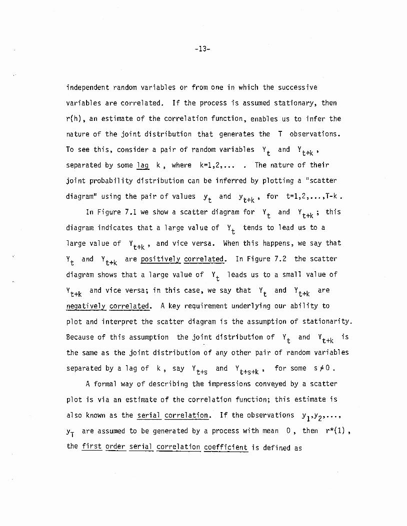
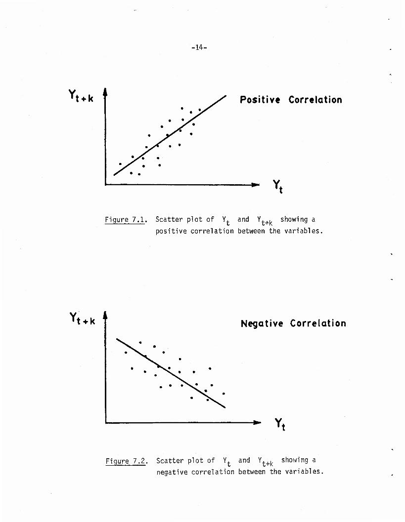
In Figure 7.1 we show a scatter diagram for Y. and Yt+^ ; this
diagram indicates that a large value of Y. tends to lead us to a
large value of Y.+k , and vice versa. When this happens, we say that
Y. and Y.+. are positively correlated. In Figure 7.2 the scatter
diagram shows that a large value of Y. leads us to a small value of
Y. . and vice versa; in this case, we say that Y. and Y.+. are
negatively correlated. A key requirement underlying our ability to
plot and interpret the scatter diagram is the assumption of stationarity.
Because of this assumption the joint distribution of Y. and Y.+. is
the same as the joint distribution of any other pair of random variables
separated by a lag of k , say Y. and Y. +. , for some s/0 .
A formal way of describing the impressions conveyed by a scatter
plot is via an estimate of the correlation function; this estimate is
also known as the serial correlation. If the observations y^y?.--.»
yT are assumed to be generated by a process with mean 0 , then r*(l) ,
the first order serial correlation coefficient is defined as
•14-
Yfk • Positive Correlation
* Y.
Figure 7.1. Scatter plot of Y. and Y.+. showing a
positive correlation between the variables,
Yf Negative Correlation
* Y,
Figure 7.2. Scatter plot of Yt and Yt+k showing a
negative correlation between the variables.

•15-
(7.1) r*(l) - t=1
T-l
I ytyt+l
I y\ t=i r
If the mean of the process is not known, (7.1) is modified by
replacing y. and y._, by the deviation of these from the sample
T mean y , where y = £ y./T . Thus we have
t=l z
(7.2) r(l) = I (yt-y)(yt+l-y)/ I (yf-y)2 . t=l z z L t=l r
Higher order serial correlations are similarly defined; for
example, r*(h) , the h-th order serial correlation is
(7.3) r*(h) = t=1
T-h
L yt yt+h
T ?
t=i z
or in analogy with (7.2) it is
(7.4) r(h) =
T-h Uyt-y)(yt+h-y)
t=i z

-16-
8. Autoregressive Processes
One of the simplest, and perhaps the most useful, stochastic
process which is used to model a time series is the autoregressive
process. A sequence of random variables y,,y?,... is said to be an
autoregressive process of order p, abbreviated as AR(p) , if for
some constant p and integer p
(8.1) (yt-y) +31(yt.1-y) + -....+ ßp(yt-p-y) = ut ' t = P+1>P+2>--- »
with u ,, u 2"*" being independent and identically distributed
with mean 0 and variance a , and u. independent of y._,, y. 2»
... . We shall set p = 0 in the following discussion. The random
variable u. is called an innovation or a disturbance. We shall refer
to the sequence {u.} as an innovation process.
It is convenient to generalize (8.1) to a doubly infinite sequence
...» y_i> yr>j y-,,..., resulting in a doubly infinite sequence ...,u_-,,
UQ,U,,... . Such processes are also known as autoregressive processes.
k def If we use the foreward lag operator p, where p u. = ut+. for
any integer k , then (8.1) can also be written as
(8.2) (pP+31PP_1+...+3pP°)yt_p = ut .
Since Ayt=yt+1 - yt = R/t"yt = ^^yt ' we have the result
that A = p-1 ; recall that A is the foreward difference operator
introduced in Section 3.3. Thus we may say that the operator acting on
y. can also be written as a polynomial in A of degree p . If u-p
(3 £ 0 , then the left hand side of (8.2) can be written as a linear
combination of yt_ , Ayt_ , A yt_ ,...»APyt_p and is therefore called
a stochastic difference equation of degree £.

-17-
Unless otherwise stated (see for instance Section 8.9), we shall
assume that the stochastic process described by (8.2) is stationary.
In Section 8.1 we shall determine the conditions under which uf is
independent of y, ,, y+.o"'" '
The model (8.1) can be used to generate other processes. For
example, should we want to incorporate the effect of a trend in (8.1),
then we add to the left hand side of (8.1) the term £ y.z.. , where
the zit's are known functions of time; this matter is discussed
further in Section 8.7.
Autoregressive processes were suggested by Yule (1927), and were
applied by him to study sunspot data. Gilbert Walker (1931) extended
the theory and applied it to atmostpheric data. In what follows we
shall study the structure of autoregressive processes, and address the
related questions of inference and prediction.
8.1 Representation as an Infinite Moving Average
If we inspect (8.1), we see that y. is expressed as a linear
combination of the previous y.'s and u. . We shall now study the
conditions under which y. can be written as an infinite linear com-
bination of u. and the earlier u 's . To see the idea, we consider
an AR(1) process
yt = pyt-i + ut *
and note that since y. , = pyt_2 + ut , , we have
yt = ut + pUt-l + p2yt-2 '
-18-
Successive substitution of the type indicated above leads us to
wri te
(3.3) yt = ut + PUt_1 + P2ut_2 + ... + PSut_s + PS+1yt_(s+l)
so that
(8.4) yt-(ut + PUt_1 + ...+P ut_s) = P yt.(s+1) •
The difference between y. and a linear combination of the
s+1 (s+1) u 's is therefore P ^t-fs+l} ' anc* t'11"s becomes sman when
|P|<1 and s is large. In particular
(8.5) e[yt-(ut + Put.1 + ...+Psut_s)]
2 = p2(s+1)eyt(s+1)
will not depend on t , if we assume that {y.} is a doubly infinite
stationary process. As s increases, (8.5) will go to 0 , and so we
can write
yt = I p ut- z r=0 c
r u.
r
and say that the infinite sum on the right of the above equation
converges in the mean to yt . (See Section 5.7.)
Let us now consider an AR(p) ,
P
4o 3^-r = Ut ' 30 = l •
so that
yt = Ut " ßlyt-l " ß2yt-2"---"ßPyt-p '

•19-
Replacement of t by t-1 yields
h-i - ut-r Vt-2 - HH-z - •••" Vt-p-i •
which upon substitution gives
yt = ut-ß1(ut_1-31yt_2-02yt_3- ... - y^p^-ß^t-z" — "Vt-p
= ut-Biut-i-(B2-Bi,yt-z- — + 0iVt-i-p •
Continuing in the above manner s times, we arrive at
(8.6) yt = V6*U1>1 + ... + <ut_s+aslyt_s_1+as2yt_s_2 + ... +^t_s_p •
We note that each substitution leaves us with p consecutive y 's
on the right-hand side of the above. Since yt_s_i =ut_s-l " glyt-s-2 "
•••"Yt-s-p-l- we have
yt = V5lut-1 + • •' + Vt-s + asl(ut-s-rtyt-s-2 •'' -Vt-s-p-lJ
+ asZh-s-2 +-" + aspyt-s-p •
- ut + Vt-1 + ••* + 6sut-s + aslVs-l + (as2 " aslßl)yt-s-2
Thus
+ ... + (a*p - a*iBp-l)yt-S-p " 4 Vt-S-p-1
ös+l = asl '
as+l,j = (as,j+l-aslßj) ' j = 1 P-1 '
* * n a,,, = -a ,p s+l,p sip

•20-
is a set of recursion relationships for the coefficients. Continuation
* of this procedure leads us to write, for 5Q = 1 ,
(8.7) y = I 6* u . t i=0 l t i
if the infinite sum on the right-hand side of (8.7) converges in
the mean to y. . We shall next see the conditions for this convergence.
8.1.1 Conditions for Convergence in the Mean of Autoreqressive
Processes
The material of Section 8.1 can be formalized by using the backward
lag operator z , where sy. = y. , , and writing the process (8.1) as
P
I 3 £ryt = u . r=0 r z z
Then, formally we can write our AR(p) process as
P
yt = ( i (v/r1 u. , z r=0 r z
where
( I e/r1 = I 6 / j r=0 r r=0 r
the 6 's are the coefficients in the equality

-21-
1
(8.8) ( l ßzT1 = I 6zr
r=0 r r=0 r
on the basis that the above equality can be so written meaningfully.
It can be verified (Anderson (1971), p.169) that the 6 's
of (8.8) are indeed the same as the ö 's of (8.7), which we recall *
were obtained by successive substitution; thus we write 6=6.
In order to see the conditions under which it is meaningful to
write (8.8), we consider
(8.9) ß0xp + 31xp-1+... + ß x°
the associated polynomial equation of the stochastic difference equa
tion (8.1) (our AR(p) process).
For 3D^0, let x,,...,x be the p roots of (8.9). If
it is clear that 7 - •P
x- j < 1 , for i = l,...,p, then it is clear that z-, z , the roots
of P I 3/ = 0 ,
r=0 r
are such that z. =l/x. and that |z. | >1 . Now, for any z such
that |z| < min|z-| , the series
(8.10) —I = —-i = n I (f) = I 6/ r !.{1.i, -1-0 ^ r=0
r^O 3^ i=1 *»

-22-
converges absolutely. Thus we see that when x.,...,x , the roots of
the associated polynomial equation of an AR(p) process, are less
P than 1 in absolute value, we can write ( £ ß zr) = I 5 zr .
r=0 r r=0 r
To argue convergence in the mean of the AR(p) process, we con-
P sider the expression ( £ ß„zr)~ and note that by a formal long
r=0 r
hand division
l ß1zfß2z2+...+ß zp
l+ß,z h...+ßnzP l+ß1z+ß2z2+..-+ßDzP
r -L r
= 1- ß,z (ß2-ß
2)z2+...+(ßp-ß1ßp.1)zp-ß1ßpz
P+1
1+ßjZ+ßgZ +...+ß zp
If we continue in the above manner, we see that
7S+1X X ,S+P „ a ,Z +...+a Z
= l+6,Z*-60Z,::+...+6 Z +— ^_ l+ßjZ + .-.+ß ZP l S l+ßjZ + .^+ß ZP
where the 6 's and the ct -'s satisfy the same recurrence relation-
ships as the 6 's and the a .'s of Section 8.1. Thus 6=6 r r si r r and a . = a . . (See 8.6.)
7S+14- 4. 7S + P a-jZ +...+a z In view of (8.10), we now see that P—-— must con-
l+ß1zf...+ßzP
verge to 0 for |z | <min|z.| , and in particular for z =1 . This i i
implies that the a . -> 0 (as s->°°) for each i . Thus, if {yt> is
•23-
a stationary process
3
£(yt~J0 W/ = £(aslyt-s-l+"-+aspyt-s-p)2
will not depend on t and will converge to 0 as s -*°°
We therefore have
yt = Jo '-ut-r
in the sense of convergence in the mean. We have proved
P Theorem 8.1; If the roots of the polynomial equation 1 &J(. = 0
r=0 r
P associated with a stationary AR(p) process Y 3 y. = u. are
r=0 r z~r z
less than 1 in absolute value, then y, can be written as an infinite
linear combination of u., u. ,, u.p»...» .
Note that whenever y. can be written as an infinite linear combi-
nation of u., u. ,,..., yf will be independent of the future innova-
tions u.+1, u.+2....s ; this follows from our assumption that the
sequence of innovations {u,} is mutually independent. We thus have
as a corollary to Theorem 8.1
Corollary 8.2; If the roots of the polynomial equation associated with
a stationary AR(p) process are less than 1 in absolute value,
yt is independent of ut+,, u.+2,..., .
-24-
8.2 Evaluation of the Coefficients 6 and their Behavior r
Suppose that the roots of the associated polynomial equation P I 3 xp~r = 0 , are less than 1 in absolute value. Then, by
r=0 r
Theorem 8.1, we can write
yt = rlQ Vt-r >
where the 6 's are to be viewed as weights associated with the present
and past innovations u., u._,,... . Our goal is to determine a proce-
dure by which the & 's can be expressed in terms of the known 3 's ,
and also to see if there is any discernable pattern in the 6 's . Such
a pattern will enable us to interpret the behavior of our sequence {yt>.
From (8.10) we note that since
CO
1 _ V * S P n r ' ¥ r=0 I 3 z
r=0 r r
or that
P P P
( I 3 zT1 I e.zs = ( I VP) l ßszS = 1 ' r=0 r s=0 s r=0 r s=0
> l wr+s = i r=0 s=0 s r
Replacing r by (t-s) and by suitable re-arrangements, we have
P-1 t - P I ( I 3sSt_s
)zt + H I 3s5t_s)zt = 1 ,
t=0 s=0 s z s t=p s=0 s z s
which is an identity in z (the series converging absolutely for
|z | <1) . An inspection of the above reveals that the coefficient of
-25-
z on the left hand side is 1 and the coefficients of the other
powers of z are zero; thus we have the following set of relationships
between the 6's and the ß's :
(8.11)
Wo = 8Q = l
Vi + 3iöo = 6i + ßi=0 '
{ 3oVi + "-+Vi5o = 0' and
(8.12) Vt + -+Vt-P = 0 t = p, p+1,..., .
We note that (8.12) is a homogeneous difference equation which
corresponds to the (stochastic) difference equation that describes the
AR(p) process
Vt + ßlyt-l + "'+Vt-p = Ut' ßn = l J0
If the roots of (8.9), the polynomial equation associated with an
AR(p) process are distinct, then the general solution of (8.12) is of
the form
P (8.13) V = I kix r = 0,1,...,
wh ere k,,...,k are coefficients 1 p

•26-
If a root x. is real, then the coefficient k. is also real.
If a pair of roots x. and x.+, are conjugate complex, then k. and
k.+, are also conjugate complex and k.xC + k-+,xr+. is real,
r = 0,1
Equations (8.11) give us the boundary conditions for solving (8.12).
The p equations (8.11) enable us to determine the p constants
k,,...,k by substituting (8.13) in (8.11).
The above material can be better appreciated via some special cases;
these are discussed below.
8.2.1 Special Cases Describing the Evaluation and Behavior
of ys
We shall consider here two examples, an autoregressive process of
order 1 and an autoregressive process of order 2.
An Autoregressive Process of Order 1
Suppose that in (8.1) p = l (and y=0), so that an AR(1) process
is
ß0yt +f3lyt-l = ut ' for t = 2>3"-- •
The associated polynomial equation for the above process is
BQX + S^ = 0 ,
and so with 30 = 1» x =-ß, is the only root.
•27-
From (8.11) we have 6«=1 and 6, =-ß, , so that the coefficient
k, in (8.13) is 1 . Thus, for our AR(1) process the coefficients
<5 are such that
(8.14) ör = kixi = ("0i)r • '
Now, if we assume that the process is stationary, then in order to
be able to write y. as an infinite linear combination of u., u. _,,...,
we need to have, by Theorem 8.1, |x| < 1 or equivalently |3-,| <1 . •
Thus, when |ß.| <1 , we can write
oo
(8.15) yf = I 5 u. . z r=0
We note from (8.14), that the weights s exponentially decay in
r when |ß, | < 1 . The decay is smooth if 3.. < 0 , and the decay
alternates in sign if 3, >0 . This behavior of the 6 's implies that
in (8.15) the remote innovations receive smaller weights than the more
recent ones. Such results are useful for explaining the behavior of
the series y., y._,,..., and also interpreting forecasts in autoregres-
sive processes or order 1.
An Autoregressive Process of Order 2
Now suppose that in (8.2) p = 2 (and u=0) , so that an AR(2)
process is
ß0yt + ßlyt-l + ß2yt-2 = ut » t = 3,4,... .

-28-
With 3Q=1 the associated polynomial equation for our AR(2) process
becomes
2 0 x + gjX + ß2x = 0 .
If x, and Xp are the roots of the above equation, then x. = (-3-,
A\ - 4ß2 )/2 , i = 1,2 .
If the roots x, and x2 are real and distinct, that is ß, >4ß2
then (8.11) and (8.12) give 1 = M? + k2x2 = k. + k2 and k^ + k2x2
= -ß. = x,+x2 . The solution is
xi _x? k, = — and k9 = —-§-
Then
xr+l_ xr+l
(8.16) 6r = ^ -x 2 ' ^ = 0,1,2,.
If we assume that our AR(2) process is stationary, then in order
to be able to write y, in the form (8.15), that is, as an infinite
linear combination of ut, u._,,..., we need to have (by Theorem 8.1)
|x.| <1 , i = 1,2 . This in turn implies that the coefficients ß, and
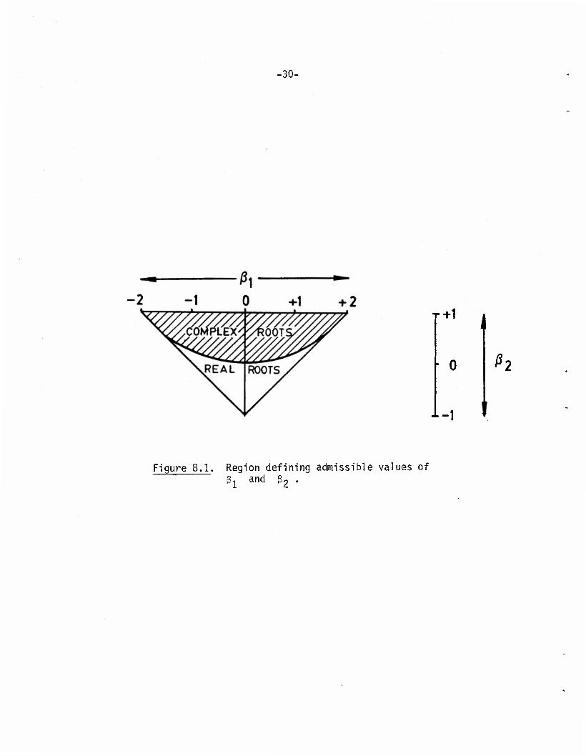
ß2 will have to satisfy the following conditions:
ß1 + ß2 > -1,
(8.17) g _ 32 < 1 , and
-1 < 32 < 1 .

-29-
Th e above conditions define a triangualr region, shown in Figure
8.1, in which the coefficients ß, and ß2 must lie^ also see Box and
Jenkins, (1976), p.59.
When |x. | <1 , i =1,2, and x1 and x2 are real, that is, when
ß. and ß2 lie outside the parabolic region of Figure 8.1, then from
(8.16) it is clear that the weights 5 are a linear combination of
r+1 r+1 two exponentially decaying functions of r, x, and x2
When |x. | <1, i =1,2, and when x, and x? are complex, that
2 is ß, < 4ß2 so that ß, and ß2 lie in the parabolic region of
i ft —i ft Figure 8.1, x» and x? may be written as x., = ae and x2 = ae ,
where i = /^T ; since |x, | < 1 and |xJ < 1 , a < 1 . Thus
J6 o"1
k, = --I ^r and k„ = "e e -e e -e
so that
(8.18) 6r = k xj + k^ = J 5 ^JL_ e - e
r sin(8(r+l)) " a sin 0
1 ft ' since e = cos e + i sin e .
Thus S is a damped sine function of r , whose nature is illus-
trated in Figure 8.2. Such a damped sinusoidal behavior of the weights
offers an explanation of an oscillatory pattern of the y.'s often
observed in otherwise nonperiodic stationary time series. (Also see
Section 8.6.)
-30-
T+1
F o
1-1 *
Figure 8.1. Region defining admissible values of 3, and 32 •

•31-
Figure 8.2. Behavior of the weights 6 as a function of r ,
for an autoregressive process of order 2 whose
associated polynomial equation has complex roots.

•32-
In conclusion, we note that for a stationary autoregressive process
of order 2, the remote innovations in a (8.15) type representation of
the series receive a smaller weight than the more recent ones, regardless
of whether the roots of the associated polynomial equation are real or
complex. The nature of the roots determines whether the weights decay
exponentially or sinusoidally.
8.3 The Covariance Function of an Autoregressive Process
If the joint distributions of the y,'s are normal, then the
process is completely determined by its first and second order moments,
2 £yt , £yt , and Sy+yt+s » s = l»2, If the joint distributions are
not normal, the above moments still give us some information about the
process. For example, &y.yf+//&yz&y^ , the correlation between yt and
yt+. (assuming that £y. =0 for all t) , is a measure of the relation-
ship between the two variables y. and y for t = l,2,...
If the process is stationary, then all the variances are the same,
and the covariances depend only on the difference between the two indices.
Thus
eytyt+s = a^ =cr(~s) ' s = •••» _1' °» +1"" •
Recall that a(s) is also called the autocovariance function and that
a(s)/a(0) is also called the autocorrelation function; it will be denoted
by p(s) and abbreviated as ACF.
We shall now look at the properties of the covariance function a(s) .

•33-
If we replace t by t-s in y. = l öu and multiply it by —n M ** H q=0
l ßryf r = u. , we have r=0 r ^ r r
(8-19) rl0 VtVt-s • qi0 Vt-s-A •
Now eyt_ryt_s = a(s-r) , eu2 = a2 , fiu^ = 0 , t^s, and so the
expected value of (8.19) satisfies the following equations:
P (8.20) I ß a(s-r) = a2 , s=0
r=0 r
(8.21) £ ß a(s-r) = 0 , s = l,2,... r=0 r
The above equations are known as the Yule-Walker equations; these will
be discussed further in Section 8.4.
From (8.21) we observe that the sequence a(l-p), a(2-p),...,
a(0), a(l),... satisfies a homogeneous difference equation, which is
the same as the homogeneous difference equation (8.12). Thus, if x, ,
P ...,x , the roots of the polynomial equation £ ß x^~ = 0 , are
p r=0 r
distinct and ß f 0 , the solution to (8.21) is of the form
P (8.22) <r(h) = I c.xj , h = l-p, 2-p 0,1
i=l 1 1
where c,,...,c are coefficients,

•34-
There are p-1 boundary conditions of the form
cr(h) = a(-h) , h = l,...,p-l ,
and the other boundary condition is given by (8.20) with a(-p)
replaced by a(p) .
Thus the behavior of the autocovariance function of an AR(p)
process is determined by the general nature of (8.22). We study this
by considering some special cases.
8.3.1 Special Cases Describing the Behavior of the Autocovariance
Function of an Autoregressive Process
Following Section 8.2.1 , we consider here an autoregressive pro-
cess of order 1 and an autoregressive process of order 2.
An Autoregressive Process of Order 1
Suppose that in (8.1) p = l (and y=0), so that
yt + ßlyt-l = ut ' t = 2,3,..., .
The associated polynomial equation x+ß-x = 0 has one root x, =-ß, .
The general solution is (from (8.22)) a(h)=c,(-ß,) , h=0,l,... .
From (8.20) we have
a2 = a(0) + 8^(1). = CjCl + ß1(-ß1)] =C1[1 - ß2] .

•35-
2 2 Hence c. = a /(1-ß.) , so that
a(h) = (-ßl)ha2/(l-ß2) s h=0,i »••• J •
From p(h) = a(h)/o(0) , the autocorrelation function is
(8.23) P(h) = (-3Jh , h=0,L
If 13-, | <1 , then we have the important useful result that the
theoretical autocorrelation function of an autoregressive process of
order 1 decays exponentially in the lag h . The decay is smooth if
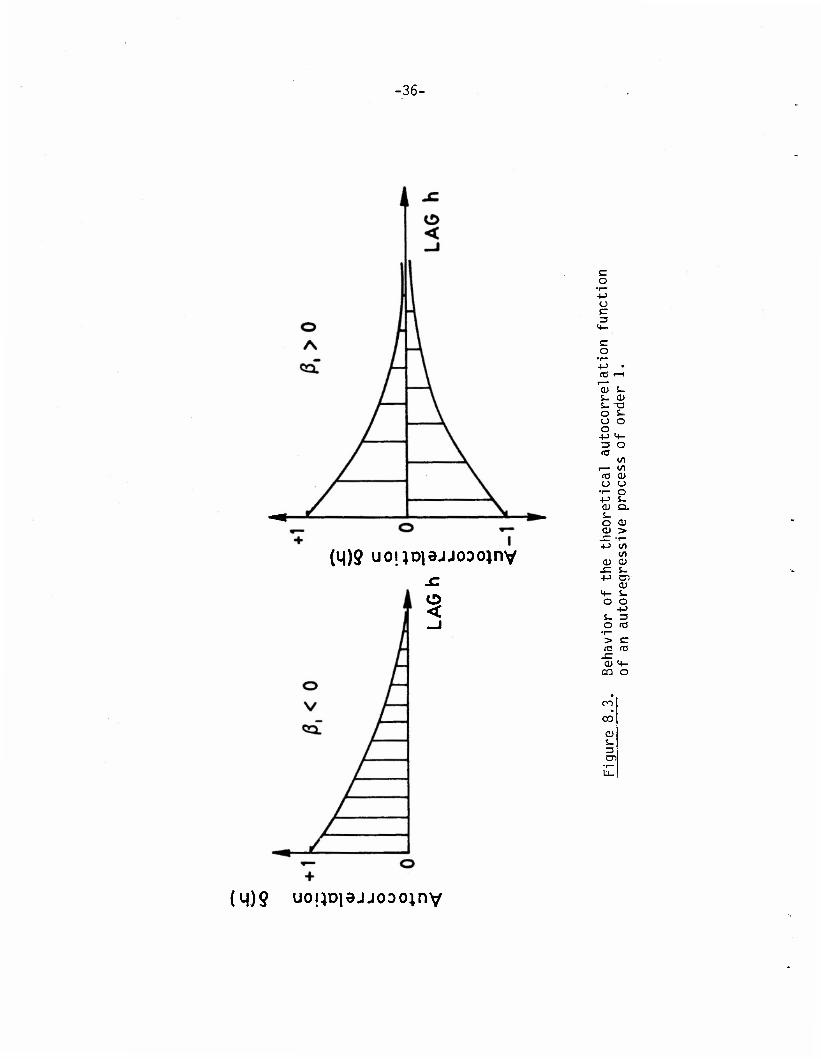
3, < 0 , and it alternates in sign if 3-, > 0 . In Figure 8.3, we illus-
trate this behavior of p(h) for nonnegative values of h . We also
remark that the behavior of p(h) is analogous to the behavior of the
weights S discussed in Section 8.2.1 - see (8.14) and Figure 8.2.
An Autoregressive Process of Order 2
Now suppose that in (8.1) p = 2 (and y=0) , so that
yt + 3lyt-l + e2yt-2 = ut' t = 3,4,..., .
2 0 The associated polynomial equation x + 3-,x + 3oX = 0 has the roots
xn- = [-ßj ±/3j-432]/2 , i = 1,2 .
If the roots x, and x2 are distinct, then a(h) =c,x!? + c2x!] ,
h = -l,0,l,... . Then (8.20) and a(l)=a(-l) can be solved for c.
and c2 , yielding
•36-
(L|)9 uojiDiejJODOinv
<
c o
•r- +J (J c 3
M-
C o
•I—
+-> • ns t—i r-
c» t- s- 0) S- T3 O 5- O O o
4-> 4- 3 o 03
10 ^~ co
res CD O U
• r— O +-> s- <u Q. S- o a> a > ^~ °r— 4J to
to CD a -C s_ 4-> D-.
ai M- S- O o
+-) S- 3 o fO
'r— > c rö CO
JE a> M-
CO O
CO
(M)§ uo!;D]ajjoooinv

•37-
2 x h+1 x h+1
(8.24) a(h)= 2 (J___2 )? h=Q^ (x1-x2)(l-x1x2) 1-Xj l-x|
If we require that |x.. | < 1 , i=l,2, then 3. and 32 must lie
in the triangular region described by Figure 8.1; that is, they must
satisfy the inequalities (8.17). Furthermore, if x, and x2 are
real, that is 3, and 32 do not lie in the parabolic region of
Figure 8.1, so that 3?>432 , then by (8.24) we have the result that
a(h) is a linear combination of two exponentially decaying functions
of h , x.. and x~ . Depending on whether the dominant root is
positive or negative, a(h) will remain positive or alternate in sign
as it damps out. This behavior of a(h) as a function of h>0 , is
shown in Figure 8.4.
When |x. |<1, T =1,2, and x. and x2 are complex, that
is, 3| < 432 , then x, and x2 can be written as x, = ae and
— 1 ft x2 = ae" , where a <1 , and now (8.24) becomes
(8.25) CT(n)=^ah[sine(h+l)-a2 sin e(h-l)] ?
(1-a )sin e[l-2a cos 2e+a ]
a a CQS(eh-(j))
(l-a2)sin 0vl-2a2 cos 2e+a4 h =0,1,...,
2 2 where tan 4> = (1-a )cot e/(l+a )

-38-
douDUDAOoo;nv
/IS t/>
o o a.
z < z •-•4
O Q
Ul >
O Ü.
/
E tO (O T-
E 4- O O E
>> E r— o o •i- Q. -t-> o -o E CU 3 +->
M- «3 •i—
CL> CJ O O E Ul tO to •r- tO S- n3 c/5 > +J o ••- O O E
+-> 0) 3 -E to 3
l~~ **
to CM O •r- S- +-> <u CU T3 S- S- o o CD .E M- S-> O •
to 0) to +-> .E to o +-> cu o
o s- o
*-» s- T—
x: a. to *^^ CD o ai s-
> • r- 10
4- to to O to -E
<u s- s- E o en o •i- cu •t—
> s- +J tO o to -E +-> 3 QJ 3 O"
CQ to 0)
co CD S- 3 C7>
(14)0 dDuouDAOoo;nv
-39-
Thus a(h) is a damped cosine function of h ; the behavior of
a(h) as a function of h = 0, ±1, ±2,..., is illustrated in Figure 8.5.
Since a(h) is a linear combination of the hth powers of the
roots x, and x? , both of which are less than 1 in absolute value,
|a(h)| is bounded. We remark that the behavior of a(h) as a function
of h is analogous to the behavior of the weights 6 as a function
of r, discussed in Section 8.2.1 - see (8.16), (8.18), and Figure
8.2.
Thus to conclude, we have the important practical result, that
when Si and ß„ , the parameters of an AR(2) process, lie in the
triangular region described by Figure 8.1, the theoretical autocorrela-
tion function decays either exponentially or sinusoidally. The exponen-
tial decay could be either smooth or alternating in sign, depending on
the values that e, and ß~ take.
In Section 8.11, we show the behavior of the estimated autocorre-
lation function of some real life data which we claim can be reasonably
well described by autoregressive processes. However, in order to be
able to use the behavior of the autocorrelation function as a means of
identifying autoregressive processes, we need to have some idea about
the behavior of the estimated autocorrelation function of some known
autoregressive processes. This we do next, and also make some other
comments which have some practical implications.

-40-
O) o C\J c (Ö S_
•i- a) i- -a to s- > o o O M- o o
«3 O
O 3 l/l'r tC (/) +J
0) (O i— O 3
o cr s- 0)
•i- Q. 4J r— ai tu is s-'o • O M- O) </>
-G t/5 +-> <u
E o c
<L> S- i— en o a> D. S- o -a =5 4->
<4- o
o • O 1/5 to +-> to O <a
5- o
c to O 4->
> 4-> i— (0 O C Q. r CUE cu 3 -c o ccit-S u
CO
dJ
-41-
8.3.2 Behavior of the Estimated Autocorrelation Function of
Some Simulated Autoregressive Processes
The results of Section 8.3.1 can be generalized in a straightfor-
ward manner to show that the autocorrelation function of autoregressive
processes must decay exponentially or sinusoidally. Even though this
result is true in theory, it is unreasonable to expect such a behavior
of the estimated autocorrelation function. Such a lack of conformance
between the theory and its application is mainly due to the sampling
variability in our estimate of the autocorrelation function (see Section
7), and is particularly acute when we are dealing with series of short
lengths, wherein our estimate of the autocorrelation function is based
on few observations. Thus a good deal of caution and insight has to be
used in order to identify the nature of an underlying stochastic process
by examining the behavior of its estimated autocorrelation function.
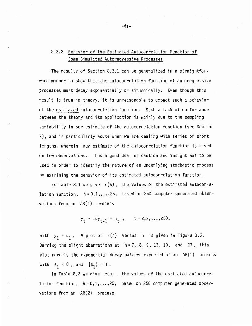
In Table 8.1 we give r(h) , the values of the estimated autocorre-
lation function, h =0,1,...,25, based on 250 computer generated obser-
vations from an AR(1) process
yt - -5yt_i = ut , t = 2,3, ...,250,
with y1 = u1 . A plot of r(h) versus h is given in Figure 8.6.
Barring the slight aberrations at h=7, 8, 9, 13, 19, and 23, this
plot reveals the exponential decay pattern expected of an AR(1) process
with ß, < 0 , and |ß,j < 1 .
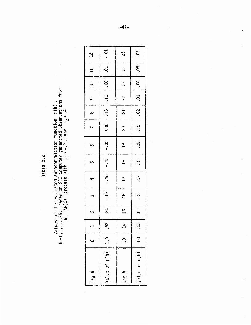
In Table 8.2 we give r(h) , the values of the estimated autocorre-
lation function, h=0,1,...,25, based on 250 computer generated obser-
vations from an AR(2) process

-42-
<3- o o
1X5 CM o
o «3- CM
1X3 O
1x3 O
CO
CD
.a (8
E o
« oo E '—. o
-E •>- —' +J
> E CU O to
•r- J2 -t-> o • O CT3U5 3 0) •
«*- 4-> I <C S- CÜ
•>- E i— -(-> CD CO. ta en
ai
co
co CM
CM CM
O CM
r-~- o
o
Ln o
<X3 o
c o
II 1X5
CD S- -E s_ CD +-> t- +-> •<- o =s 2 u a. o E </i +-> o oo 3 O CD IB o
o o -o LT3 S_
CÜ CM a. +-> <T5 E E O-^
•r— 1—<
+J T3-— to CD C£ CD to <C
fO CD -Q -E E 4-3 (0 ft <+- LT3 O CM
ft
on * CD •
^1- o
*3- O
CTt O
1X3 I-H
CO CO
1X3 1X3
00
1X3
03 CO o
co o
CM CM o
o co o
co o
o II CO
oo o
O
CD
4- O
CD
CD CT. to

-43-
^ I C
a
o o
o £ V) UJ
1.0
0.8
0.6
0.4
0.2 Y
0.0 I I I I I I i i » I i I t i i I 1 i i 1 i 01
4- 10 15 20 25 LAG h
Figure 8.6. A plot of the estimated autocorrelation function r(h) versus h, h = 0,1, ,25,. based on 250 computer generated observations from an AR(1) process with 3-, = -.5 .
-44-
£ o i_ 4-
„ </) c
-—•> o x: -I- *—- -4-> <d" S- (B •
t » C CD CM O o a
•i- _Q +-> o O "O c -a c =s a) re 4- •(->
,.. * .. — s- a cu cr>
•r- E • +J a) 1 CO D) || ^"—
CM a s- i-H • S- CD ca cn S- +->
O 3 <u o o.x:
i—° O E +J X) -P O -r- CO 3 O 2
I— CO O CO
"C IX) CO CD CM CU
•P O (O E O E o &- •t- Q. •PTI CO CU a oo—^
CO CM OX)-^-
-£= a; •P ca:
A
4- IX) O CM C
« CO CO . cu .
o II
CM .—1
r—1 o IX)
CM «XI o
i-H LT) «—I
.—1 o CM o
to CO CM
"=3- O I-H
o o
CT) CO <—1
CM CM
r-l O •
IX) t-H CM CO I-H CM O
'
CO IX) r~» 00 O o o CM
'
•X)
CO o Ol o •
CO IX) IX)
I—1
1
CO i—1 o •
to CM C3-
1
O
co o <X> i—I
o o
«tf- ix> 1—)
CM CM o
CO •=3- I—H
CO I-H vo o
o o CO CO
o t—1
_ ^ x: x:
S- %. 4- li- o CS
JC cu x: CU 3 3
CD i— cn r—
CO CO CO CO _l > _j >
-45-
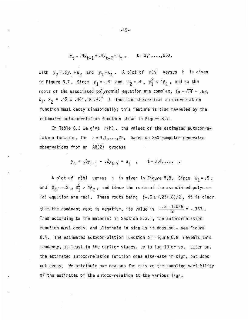
yt" ,9yt-l + -4yt-2 = Ut ' t = 3,4,...,250,
with y„ = .9y1+u2 and y. = u, . A plot of r(h) versus h is given
in Figure 8.7. Since ß,=-.9 and ß2= -4 , ßj < 4ß2 , and so the
roots of the associated polynomial equation are complex. (a = SÄ = .63,
Xp x = .45 ± .44i, 9^45° ) Thus the theoretical autocorrelation
function must decay sinusoidally; this feature is also revealed by the
estimated autocorrelation function shown in Figure 8.7.
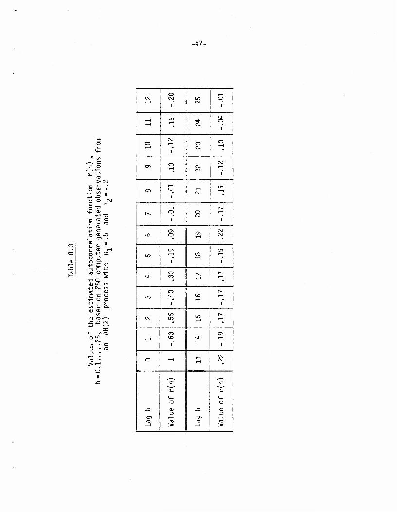
In Table 8.3 we give r(h) , the values of the estimated autocorre-
lation function, for h=0,1,...,25, based on 250 computer generated
observations from an AR(2) process
yt + -5yt_i " -^-2 = ut ' t = 3,4,..., .
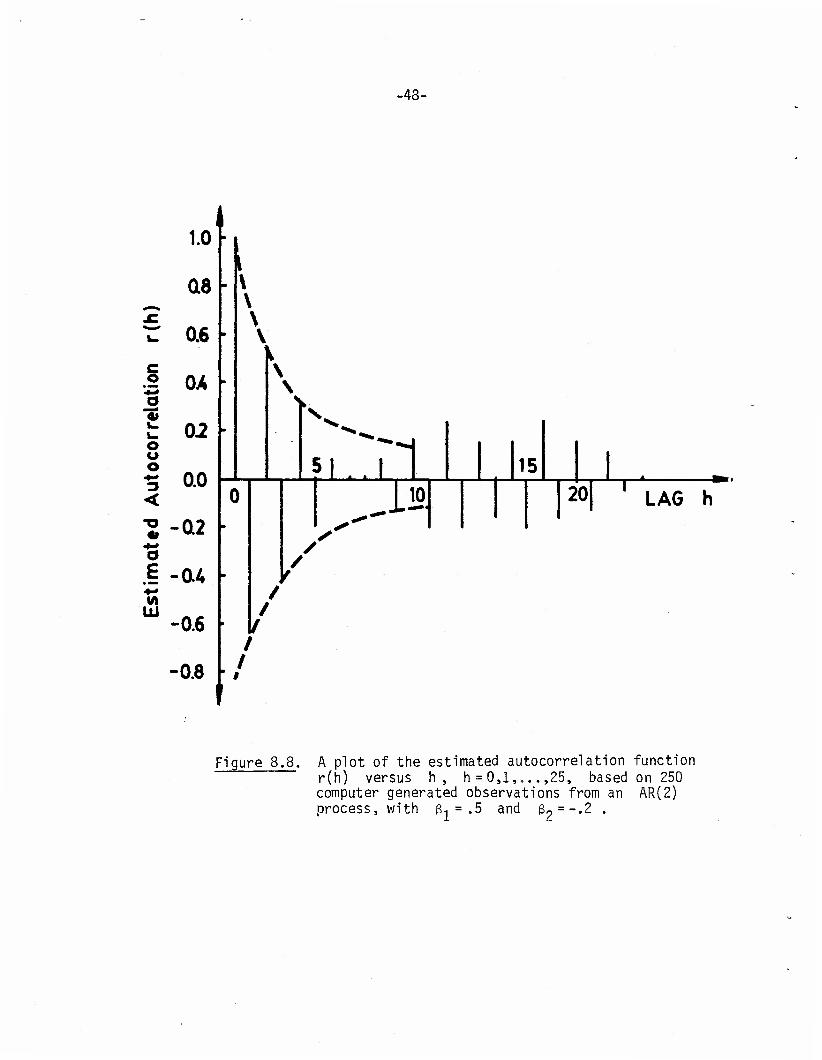
A plot of r(h) versus h is given in Figure 8.8. Since ß, = .5 , 2
and ß2 = -.2 , ß, > 4ß? , and hence the roots of the associated polynom-
ial equation are real. These roots being (-.5 ± /.25+.8)/2 , it is clear
- 5 - 1 025 that the dominant root is negative, its value is —: j- = -.763 .
Thus according to the material in Section 3.3.1, the autocorrelation
function must decay, and alternate in sign as it does so - see Figure
8.4. The estimated autocorrelation function of Figure 8.8 reveals this
tendency, at least in the earlier stages, up to lag 10 or so. Later on,
the estimated autocorrelation function does alternate in sign, but does
not decay. We attribute our reasons for this to the sampling variability
of the estimates of the autocorrelation at the various lags.

-46-
C
JO
o u o 4-*
<
'S £
Ixl
1.0
0.8
0.6
(U
Q2
0.0
•0.2
\
t]7 ill K • I t . • • I I | I • I I | -^ 10 15 20 25 LAG h
-0.4
t
Figure 8.7. A plot of the estimated autocorrelation function r(h) versus h, h = 0,1,... ,25, based on 250 computer generated obervations from an AR(2) process with ß, = -.9 and = .4
-47-
co CO
a; r— -O rt3
o S-
1+-
»I co ,. v E -C o — - •r-
S- 03 > CM
E s- • O a> 1
•r— co II +-> -Q
o O CM E ca 3 -o
<•- OJ +-> T3
E res E c S- 03
OJ +-> E 03 OJ IT)
CD • OJ || 5- S- S_ CU i—1
o -P CO.
CJ 3
o Q. +J t- -E
3 O +-> 03 (J •r—
s -c o OJ LO CO -p CM co o? cu E E o
o o +-> s- in T3 Q- OJ OJ
CO
OJ re .E-Q CM +J
C£ 4- fl •=r o LO
CM co A E OJ • 03 3 •
o II
sz
CM i—1
O CM
CM
t—1 o
i—1 t—1
CO i-H • CM
<* o
1
o I—)
CM r—1 CO
CM
o 1—4
CX> o t-H CM
CM
CM I-H
1
CO
I—1 o
1
i—1 CM
LO I—1
r~~. i-H o
1
o CM
i-H
1
«3 o ai i-H
CM CM
LO
CT) i—i co
i—i
CTl i-H
1
•=3- o CO i-H
I-H
CO
o CO i-H
i—1
1
CM co LO LO
i—f
1^ I-H
i-H
CO CO
i i-H
CTl
O i-H CO I—1
CM CM
.E
CD 03 _l
-E
S-
4- O
cu
03 >
JE
03 _l
-E
S-
C|-
O
CU
03 >
-48-
1
O "3» i_ k. o u o *•»
<
« 4-* O £ •-» v» u
1.0 • i
0l8 - \ V \
06 • V ' \
0A • \ <
02 • ">^^^
f\t\ 5| .. 1 15 U.U "
02 •
0 •
20| ' LAG h
/ /
0.A - f / /
0.6 • f /
0.8 • / 1
Figure 8.8. A plot of the estimated autocorrelation function r(h) versus h , h=0,1,...,25, based on 250 computer generated observations from an AR(2) process, with 3-, = .5 and = -.2
-49-
Th e behavior of the estimated autocorrelation function of some real
life data which we feel can be reasonably well described by autoregressive
processes is shown at the end of this section, in 8.11.
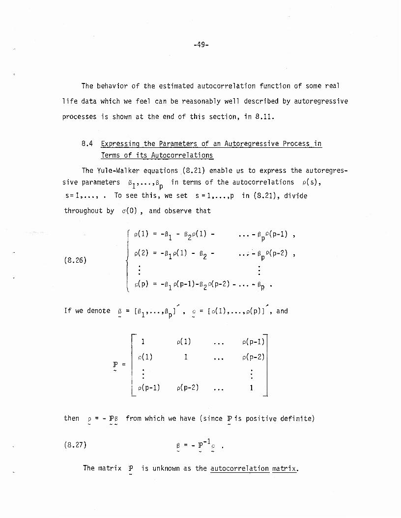
8.4 Expressing the Parameters of an Autoreqressive Process in
Terms of its Autocorrelations
The Yule-Walker equations (8.21) enable us to express the autoregres-
sive parameters ß,,...,ß in terms of the autocorrelations P(S),
s=l,..., . To see this, we set s = l,...,p in (8.21), divide
throughout by a(0) , and observe that
(8.26)
r P(1) = -3j_ - ß2P(l)
p(2) = -ßlP(l) - ß2
.. -3 p(p-l) ,
..-y(p-2) ,
p(p) = -ß1p(p-l)-ß2P(p-2) - ...- 3 ... Mp .
If we denote ß = [3,,...,3 ] , p = [p(l),...,p(p)] , and •V X [J «,
P =
1
P(1)
P(l)
1
)(p-l) p(p-2)
P(P-1)
P(P-2)
then p = - P3 from which we have (since Pis positive definite)
(8.27) 3 = - P-1p
The matrix P is unknown as the autocorrelation matrix.
• 50-
Th us, the p autoregressive parameters can be expressed in terms
of the p autocorrelations p(l),..., p(p) . This feature can be used
to estimate ß , using an estimate of P 2
We obtain a , the variance of the
a(-r)=a(r) in the Yule-Walker equation (8.20) to obtain
2 We obtain a , the variance of the disturbance, by setting
(8.28) ßQa(0) + 8^(1) + ... + Spa(p) = a2
8.5 The Partial Autocorrelation Function of an Autoregressive
Process
In Section 8.3 we have shown that a(h) , the autocovariance func-
tion of an autoregressive process of order p, is infinite in extent.
Thus from {a(h)} it is hard to determine the order of an autoregressive
process. The partial autocorrelation function, to be discussed here,
will help us in determing the order of an autoregressive process.
To be specific, let us consider a stationary autoregressive process
of order p
yt= ut - ßiyt-i ••••"Vt-P' t = p+1'p+2'--- •
Recall that in order to predict y we need consider only the p
lagged variables y. i»---»yt_D» since the other variables yt_D_i»
y-t-D-2'"" 'iave n0 e^eci on y+ •

•51-
The partial autocorrelation between y. and y._ , to be denoted
by -rr(p) is the correlation between y. and y. when the interme-
diate p-1 variables yt_,, y,_~ ^t-D+1 are "ne^ fixed." That
is, TT(P) is the correlation between y. and y. when the interme-
diate variables are not allowed to vary and exert their influence on the
relationship between y. and y. . Clearly, TT(1) , the partial
autocorrelation between y. and y._. , is p(l) , the (ordinary) auto-
correlation between y, and y._. , whereas TT(0) the partial autocor-
relation between y. and itself is 1.
Thus, by its very nature, since y, ., y^n-?""' ^ave no
effect on y , the partial autocorrelation function of an autoregressive
process of order p, TT(J') f 0 , for j =0,1 p, and ir(j)=0, for
j>p. The fact ir(j) vanished for j > p+1 , can be used to identify
the order p of an autoregressive process, provided that ir(j) can be
computed.
In our discussion of the partial autocorrelation function -n-(p) we
had mentioned the fact that the intermediate values y._, , ...,yt +-,
had to be "held fixed". In order to formalize this notion we shall use
some results which are standard in multivariate analysis.
Let Y = [y., y._,,...>yt_D] denote the vector of p+1 observa-
tions, and let z denote the variance-covariance matrix of these p+1
observations. Suppose that Y has a multivariate normal distribution
with mean vector 0 and covariance matrix z , where

-52-
E =
a(0) a(l)
a(l) a(0)
a(p)
a(p-l)
a(p) a(p-l) ... a(0)
Let us rearrange the elements of Y , and partition it into two
component sub-vectors Y^ ' = [yt, yt ] and Y^ ' = [yt_1, yt_2"-"
y^.n+il • Let E,,, E22> and £ 12 ^e ^e variance-covariance matrices
of Y^, Y^, and Y^ and Y^ respectively. That is, in, E22,
and Ej2 is a partition of the rearrangement of E . (2) ~ (?)
Let yv ' be a particular value taken by the vector Yv ' . Then,
it can be shown [Anderson (1984), p.28] that the conditional distribu-
tion of Y^ ' qiven .\r ' is a multivariate normal with mean E,0E" " given y
and covariance matrix E
12 i^ -1
11 "E12E22E12 = s 11-2 ' say* Thl'S is a 9enera",1'~
zation of the results mentioned in Section 6.
-1 (2) The vector i.^L^o yx ' is called the regression function of the
regression of Y^ ' on y . The matrix E,, « ""s a 2x2 matrix
whose elements are indicated below:
Ell-2
att.(t-l),...,(t-p+l) at(t-p)-(t-l),...,(t-p+l)
a(t-p)t.(t-l),...,(t-p+l) a(t-p)(t-p).(t-l),...,(t-p+l)
The partial correlation between yt and y holding (t-1),...,
(t-p+1) fixed at y^ is
-53-
:(P) at(t-p)-(t-l),...,(t-p+l)
/CTtt.(t-l)...(t-p+l) /a(t-p)(t-p)-(t-l),...,(t-p+l)
note that ir(p) is independent of y .
As an example, if Y = (yt> y^, yt_2)\ and if Y^ - (yt» yt_25'
(?) and Yv ' = y. , , then the partial correlation between y. and y. 2
TT(2) 5 turns out to be
*(2) = (p(2) - p2(l))/(l-p2(l)) .
8.5.1 Relationship between Partial Autocorrelation and the
Last Coefficient of an Autoregressive Process
An interesting relationship between ir(p.) , the partial autocorrela-
tion of y, and y. , and 3 , the last coefficient of an autoregres-
sive process of order p, can be observed. This relationship simplifies
our calculation of ir(p) , since 3 can
Yule-Walker equations via equation (8.28)
In order
AR(2) process
our calculation of ir(p) , since 3 can be easily obtained from the
In order to see a relationship between ir(p) and 3 , consider an
*t = Ut " 3lyt-l - ß2^t-2
and solve the resulting Yule-Walker equations to obtain

•54-
1 p(l)
p(l) P(2) _ P(2)-P2(1)
1 P(D 1-P2(D
p(l) 1
2 2 However [(p(2) - p (1))/(1 -p (1))] is indeed the partial autocorrela-
tion between y. and y._2 ; thus TT(2) = -ß« . In a similar manner,
if we consider an AR(3) process
yt = ut - ßlyt-l " 32yt-2 - ß3yt-3
and solve the resulting Yule-Walker equations, we observe that
1
P(D
P(2)
P(D
1
P(D
P(1)
P(2)
P(3)
1
P(D
P(2)
P(D
1
P(D
P(2)
P(D
1
which again can be verified as the negative of the partial autocorrela-
tion between y. and y. - .
In general, we observe [Anderson (1971), pages 188 and 222] that
for an autoregressive process or order p , ir(p) the partial autocorre-
lation between y, and y, is -ß , where Jt t-ü p '

• 55-
(8.29) ßp =
P(l)
1
P(D
P(D
1
P(2)
P(1)
p(p-l) p(p-2) p(p-3)
P(l)
1
•(p-1) p(p-2)
P(2)
P(1)
-(p-3)
P(D
P(2)
p(p)
p(p-D
p(p-2)
It is helpful to remark that the determinant in the denominator is
simply the determinant of the autocorrelation matrix for an AR(p)
process P (Section 8.4), whereas the matrix in the numerator is P
with the last column replaced by p(l),...,p(p) .
An expression for TT(j) the partial autocorrelation between y,
and y. . , can be obtained if we write the Yule-Walker equations for j ,
and set TT(j) = g. , where s. is given by equation (8.29); recall that
ir(0) =1 , and that ir(l) =P(1) .
The partial autocorrelation function is a plot of -n-(h) versus h ,
h = l,2 ; the partial autocorrelation function is abbreviated as
PACF.
We estimate TT(1) by r(l) , and estimate TT(j) by ir(j) , where
ir(j) is obtained by replacing the p(«)'s in (8.29) by their estimates
r(-)'s.
•56-
8.5.2 Behavior of the Estimated Partial Autocorrelation Function
of Some Simulated Autoregressive Processes
Even though the partial autocorrelation function of an autoregres-
sive process of order p must theoretically vanish at lags p+1, P+2,
..., it is unreasonable to expect such a behavior of the estimated
partial autocorrelation function. The reasons for this are analogous
to those given for the behavior of the estimated autocorrelation func-
tion - see Section 8.3.2. Thus caution and insight must be used when
identifying the order of an autoregressive process by examining its
estimated partial autocorrelation function.
In Table 8.4 we give Tr(h) , the values of the partial autocorre-
lation function for h=0,1,...,25 based on 250 computer generated
observations from the AR(1) process
yt-.5yt_1 = ut , t = 2,3,... ,
discussed in Seciton 8.3.2.
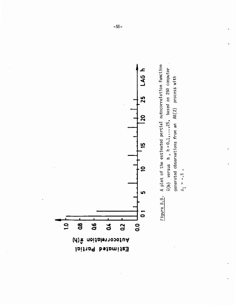
A plot of T?(h) versus h is given in Figure 8.9. Barring some
slight aberrations at a few lags, this plot reveals the behavior that
we expect from the PACF of an AR(1) process, namely that ir(l) must be
significantly different from 0 , and that TT(J) , must be close to 0
for j = 2,3,..., .
An examination of Figures 8.6 and 8.9 reveals the desired result
that for an AR(1) process, the autocorrelation function decays expo-
nentially, and that the partial autocorrelation function vanishes after
lag 1.

-57-
M E *-~^ to -C ^„* E <E= O
E <+- O
•r— to +-> c O o C •i—
3 •»-> <+-
> C s- o dl
•r- 10 +-> -Q CO O
r— Lf) 01 T3 • s- ai i S-
CO o o 5- r- o CU CO.
"3- -p c • 3 ai 00 (0
CD r— t. ••- ^~ CO a> s -Q •r— +J
CO +J 3 to 1— s- O. CO
r0 E <U Q- o o
o o T3 s- <U C Q-
+-> O CO E -a-—»
a> i-H +J CO —- 10 (0 C£ CD -Q <C
0) _s= n
-t-> CM
q- «i
o • </i * a; n
3 t—1 ^— «i
to o > II
CM i—1
00 o
i CM
CO o
i—1 r-1
CM O CM
CO o •
i
O i—1
o • CO CM
oo o •
a> C\J o CM
CM
o o
co CM o x—1
CM
CO o
r~» 1-H T—I O
CM
1—1
• 1
i£> CM O •
C7> i—i I—1
un o 1
00 I—1
I—I o
«d- CO o •
r-. i-H
CM o
co O CO t—1
I—1 o
CN1 CO o CD
I—1 o •
1
f—1 to •=d- i—i
co o
i
o i—1 CO t—1
CO r-H
CT> re
sz
< t=
o
a> 3
> re _i
< t=
M- O
a; 3
CO >
-58-
1
o
0) S-
CD
-•
o • s 3 C c
3 S
<
o
in
..©
u>
|Dj|J0d P»|0UJUS3
E O s- •r— Cü
O 3 c d. s: 3 E +->
4— o o '5
o o CO •J—
ID CO +-> CM Cl n3 o i^ c o
CD o S- S- Q- S- -o o 0) o to ^-~N
o (O CM +-> ja ^—^ 3 OL re
«V
<C ^~ LT5 rö CM C
•i— n CO -P S- # E <e , o OL A S-
r-1 M- T3 A <D o co (O II o E ,_
•r- •^•" 4-> -P ^ (0 CO > o -c
CU 0) CO .c 10 -Q +J 3
CO O
t- s- T3 o cu tu > +•> +-> fO o S-
r— ^"^ cu Q. -C c *»—^ 0)
«C <t= en
CO

-59-
In Table 8.5 we give -rr(h) , the values of the estimated partial
autocorrelation function, for h=0,1,...,25, based on 250 computer
generated observations from the AR(2) process
yt-.9yt_1 + .4yt_2 = ut , t = 3,4,..., ,
discussed in Section 8.3.2.
A plot of Tr(h) versus h is given in Figure 8.10. As is to be
expected, barring some minor aberrations, TT(1) and TT(2) are signi-
ficantly different from 0, and TT(j) is close to zero, for j=3,4,...,.
In Table 8.6 we give Tr(h) , the values of the estimated partial
autocorrelation function, for h = 0,l 25, based on 250 computer
generated observations from the AR(2) process
yt + .5yt_1 - .2yt_2 = ut , t = 3,4
discussed in Section 8.3.2. A plot of TT(II) versus h is given in
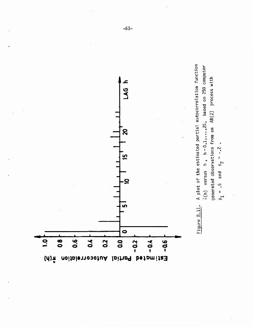
Figure 8.11. Once again, as is to be expected, -rr(l) and 7r(2) are
significantly different from 0 , and TT(J) is close to zero, for
J — o ,4 ,...,.
An inspection of Figures 8.7 and 8.10, and Figures 8.8 and 8.11,
reveals the desired result that the autocorrelation function of an
AR(2) process decays either exponentially or sinusoidally, whereas the
partial autocorrelation function vanishes after lag 2.
The behavior of the estimated autocorrelation function and the
partial autocorrelation function of some real life data which we believe
can be reasonably well approximated by autoregressive processes is shown
in Section 8.11.

-60-
CM
ID O
O CM
co O
* o S-
2*- ^£
o
EE • o « Eg:*. u a> ., c SI » l? XI c\
S-a ° o-o ea s_
"^T cu fV ccn *- a> • fe»; Ü s_ II
LO R. <u «- « tf 4-> CO. 00 5 =» (O Q_
<1> E JC f— ^ o •|-)
S3 ea
r— 2 lf> Ul £ CM 10 °- CD
-^-c s= o
* 0) S CO J3 to-—- "•"^ JD CM to •"" 0) Q;
5~c M- : * o .
A
cu ^1 =>o <o ii
a>
CO
vo
oo
CO o
CM o
o I
CT> o
to o
CM o
o
o
CO
oo CM
CM CM
o
o CM
CO
o
oo 1—1
I
o
oo o
oo o
o
CM 1-H
I
CTi o
< t=
4- o CD 3
ea CD ea
4- o Cll 3

•61-
2 1.0 Is
0.8 C o •*£ ,o 0.6 0» k. t_ O o <U o *rf 3 < 0.2
o r 0.0 a Q.
"O -0.2 • •* o E -a*
4-* (A id -0.6
f
• •»» -i1-0! I i -nl.l 1 • 15 20 LAG h
Figure 8.10. A plot of the estimated partial autocorrelation
function u(h) versus h , h = 0,1 25,
based on 250 computer generated observations
from an AR(2) process with ß, = -.9 and
0o = .4 .

-62-
io i-H CM o m o i-H
1 CM
E
I—1 i—) o CM o
LO CO o * O o o CO
,_ S- r—1 • CM .= <•- 1
<t= <2
tion
vatior
2 .
CD o 7—1 •
CM CM
CM o
1
func
bser
CO o • i-H CM
CO o •
1 O CM
«= -r. ^ ° 0) J3 •*-» "O
1-^ O • O CM
r-. o
orrela
gene
ra
.5
an
«3 o i
CM T—(
U j_ II R CU T—1 % 4-> ca
U3
00 LT> to o •
CO I—1
CO o 1
_ E-C « O -t-> -Q
(O
parti<
250
c es
s wi
LO (— <* o •
i ?—i o
imated
sed
on
proc
CO CO o i-H
o • 1
t; -a CM CM CM LO 1—4
o <" « ^-1 •
1
Tj CM i-H
CO
1—1
LO o
© : 1
0j r_' O 1—1
CO t—l O •
fO ||
> -=
< 1=
o
<!=
O
Jd aj 3
-C a> 3 en r— 05 !—
n3 (0 fB n3 _J > _l
>
-63-
1
m-L
<
tn
_o
- m
vo <* 01 rsi •*e %o Ö o c*
1 i 1
(qU uoip|»jjODO)nv pipod P»l°wu$3
o 0) •r—
O 3 a. E o o
sz 3 4->
o o IS) CO
•T— CM CO a)
tO c o "a! o o
s_ S- o o
-a cu co (O -0
O-
o <NI
3 C^ to •=£
r— CM to n C *r-
" to +J s- m E IO ^ o Q. rH s-
A ^- • T3 O <s> CM -t-> II c to E JZ o
•r- 1
•I— +J II +J A to CO > CM <D x:
cu cn
<u CO -E </) -Q T3 +J 3 O C
CO to <*- s- T3 O cu CU > -P LT> +-> to • o s- ^— *"~* <D II Q. -E c *—^* 0> .—1 < < 1= cn ca
00
a> s- 3 cn

•64-
8.6 An Explanation of the Fluctuations in Autoregressive Processes
A typical time series described by an autoregressive process fluc-
tuates up and down with oscillations which are not regular, but whose
average length depends on the nature of the underlying difference equa-
tion. We can offer an explanation of these fluctuations by considering
the representation
CO
yt = 4o 6rUt-r
and noting that
Vq = Vs+q + Vs+q-1 + '«' + 6qUS + 6q+lUS-l + ''" "
Thus, a given u will influence a subsequent y . via the coeffici-
ent 5 . In Section 8.2 we have pointed out the circumstances under
which the coefficients 5 oscillate, causing fluctuations of the
successive y 's . To illustrate this point we show in Figure 8.12, a
plot of a time series comprising of 100 observations generated on a
computer by an AR(2) process
yt-•9yt_1 + .4yt_2 = ut , t = 3,4,..., .
This is the process considered in Sections 8.3.2, and 8.5.2. Since
ß,(=-.9) and ß2(='4) a^e such that e, < 4ß2 , the roots of the
associated polynomial equation are complex with 0=44.68°, and a = .634
(Section 8.2.1). Thus the coefficients 6 will have a damped
•65-
sinusoidal behavior of the type indicated in Figure 8.2. Substituting
the above values of 0 and a in (8.18), we observe that 6, =.899,
62 = .409, <53 = .008, <54 = -.156, <$5=-.144, 5g=-.06, 67 = -.003, 6g = .025,
6g = .023, and <5,Q = .011 ; the remaining values of 6 , for r>l are
all less than .002 and are thus essentially 0 . It is because of the
above behavior of the & 's that the observations y. fluctuate up and
down about 0 with an average length of oscillation of about length
10 - see Figure 8.12. It is also useful to keep in mind Figure 8.7, the
estimated autocorrelation function of the generated series, and note
that the estimated autocorrelations for lags greather than 10 are, barr-
ing sampling variability, essentially small.
8.7 Autoregressive Processes with Independent Variables
Suppose that there are m independent variables z,.,..., z
that are known to affect the time series {y.} , t = 1,2, , being
investigated. The effect of these m variables can be incorporated
into an AR(p) model, by writing
K m (8.30) I O + I Y z. = u , t = p+l,... ,
r=0 ni r i=l ' l
where y-,,...ty are constants. It is of interest to compare the
model (8.30) with the classicial regression model (2.1) of Part I.
Let x,,...,x_ be the roots of the associated polynomial equation A P p
of the stochastic difference equation I ß y+ = u. , t = p+l,..., .
r=0 r t-r z

-66-
VI
e/i c o -p ra > S- QJ t/)
J3 O
-a CU -p . A3 S- +J CO =5 c CO II en
CM s. i (1) +J +1 >. GL • E o + o
1—1 O I O 4-> •"-" >>
I s- O 4J
>^ -s= (/>
CO 1/5 -Q CO
O CO o
-C s- 4-> O.
S= CM •r- *^^ S e; o <c
JC to
E O
•5.1 s_
< 4-
CM
CO
CO
o>
-67-
Then, using the forward lag operator p, where psy.=y. P I B„y* „ can also be written as
r=0 ^r'r
(8.31) I B_yt. = I ßrPP*ryt-D
= h (p-x..)yt.D r=0
r r r r=0 r r p 1=1 1 r p
In terms of the operator z , the above becomes
P P ( I 3_£S)y. = n (p-x.)y , s=0 s z i=l 1 t_p
or P s 1 P 1
Thus, for t = p+l, p+2,..., the model (8.30) becomes
p m ut = n (p-x.)yt_ + J yizn z j=l J z p i=l n ir
p m p = n (p-x.)[yt + I Y,-( n (P-X.)) zi + ]
j=l J T"p 1=1 n j=l J 1X
P m p . = n (p-x.)[yt + I Yi( I 3 £s)_i z. ]
j=l J x p i=l s=0 s 1st p
Before proceeding further, it is helpful to recall a result that
we have encountered in Section 8.1.1, namely, that
P 1 CO
(I s/r1 = i 6/ , r=0 r r=0
where the 6 's are the coefficients in the equality
-68-
( I ß^T1 = I V
see (8.8). Using the above, we now write IT as
ut = n (p-x.)[yt + I Yi I 6 £ z. ] t ,=1 j t p i=1 i s=0 s i,tp
j^J^t-p^I/s^l.t-p-sJ
or
r m oo
(8.32) u = I 0 [y + I Yi I 5szi t ] , r r=0 r *• r i=l ' s=0 s ''L s
since
P P
A special case of the above is our AR(p) model (8.1). To see
this, suppose that m = l, and that Z.. = 1 , for all t. Then (8.32)
becomes
P (8.33) l ß(y -p) =ut , t = p+l, p+2,... ,
where p = -y-, £ 6 . 1 s=0 s

-69-
8.8 Stationary Autoregressive Processes Whose Associated
Polynomial Equations Have at Least One Root Equal to 1
Much of our discussion thus far, has been based on the requirement
£ r that all the roots of the associated polynomial equation I 3 x = 0
p r-° of an AR(p) process l ß £ry+ = u+ , t = p+l, p+2,..., be less than
r=0 r z z
1 in absolute value. We have also assumed that the sequence of random
variables y-i,y?,... described by the AR(p) process be stationary.
In this section, we investigate the implications of allowing the abso-
lute value of one or more roots of the associated polynomial equation
take a value equal to 1 and still maintain the requirement that the
underlying sequence of random variables be stationary.
We begin by considering a stationary autoregressive process of
order 1 with its single root taking a value 1; thus we have
yt =yt_1 + ut , t = 2,3,... ,
or
Ay. * = u. , t = 2,3,... .
Thus the first difference of our autoregressive process of order 1 with
its single root equal to 1, is described by an innovation process. This
2 2 latter process is stationary. We let eu. =0, and eu. = a for all
values of t .
Now for all s > 0 , we note that
yfyt-s =ut + ut-l +-"+ut-s+l

-70-
so that
£(yt"yt-s)2 = &t + £yt-s - 2£ytyt-s = SG2 •
2 2 Since our sequence {y.} is stationary, £y. = £yt_s » and so
2 sa2 eytyt_s = a(s) = gyt - -y- , s = l,2,...,.
2 The above result can hold for all s>0 only if a = 0 , in
which case y. = y. , with probability 1.
To generalize, we consider a stationary autoregressive process of
order p , p>l , and allow one root, say x, to equal 1 , and require
that the other p-1 roots are less than 1 in absolute value; that is,
|x.| < 1 , i =2,...,p . Following (8.31), we may write our stationary
AR(p) process as
(p-1) n (p-x.)yt _ = u, i=2 c~" '
If V
we let _n (P-x-j)yt_p = zt_1 , then our AR(p) process can be
written as (p-l)zt_1 = ut , or since (p-1) =A , we have AZ. . = u. .
It now follows from our previous discussion of the stationary
AR(1) process with a single root equal to 1 that for all s>0 ,
zt = zt_s = z , say. Thus
P n (p-x.)ytm i=2

-71-
and yt = S^.g Sz , so that y+=yt_s » with probability 1 . We
therefore have as
Theorem 8.3: If a stationary autoregressive process of order p has
at least one root of its associated polynomial equation equal to 1 ,
then all values of the process are the same with probability 1 .
8.9 Some Linear Nonstationary Processes
We shall now introduce a type of nonstationary stochastic processes
that are suitable for describing many empirical time series. Such series
behave as though they have no fixed mean. The stochastic processes
introduced here, are within the general structure of autoregressive
processes.
Suppose that a nonstationary sequence of random variables y-,,y?,
is described by a stochastic difference equation of order p+d ,
so that (Pp+d + ßjpP*0-1 + ... + ßp+d-p°)yt_p_d = ut » t = p+d+l ,
p+d+2 or equivalently, the sequence is described by an autoregres-
sive process of order p+d , where
p+d
l ßr/yt = ut , t = p+d+l, p+d+2,.. r=0 r z z
P+d +d The associated polynomial equation l ß xH = 0 of the above
r=0 r
process has p+d roots x,,...,x ,x , x . . Suppose that d of
these roots, say xp+1»-••>
xp+d are exactly equal to 1 , and that the
remaining p(^1) roots x,,...,x , are less than 1 in absolute value.
Then, following (8.31), we can write our AR(p+d) process as
•72-
.ni(i>xi)(pl)dyt.p.d = "t
or
(8.34) _n (P-X.) Adyt.p_d = ut , t = p+d+l, p+d+2
since p-1 = A .
If we let w, . = Ady. . , and assume that the differenced t-p-d -'t-p-d '
sequence {w._ _d> , t = p+d+1, p+d+2,..., is stationary, then for
p>1 (8.34) becomes
(8.35) n (p-x.)wf n H = u. , t = p+d+l, p+d+2,
Thus for p >1 our model for the nonstationary sequence {y.} ,
t = l,2,..., is one for which {wtd} , t = p+d+1 , p+d+2,..., its
d-th difference is described by a stationary autoregressive process of
order p . Since the roots x,,...,x , are assumed to be less than
1 in absolute value, all our previous results for stationary autore-
gressive processes are also applicable for the model (8.35).
When p = 0 , and d = l , the first difference of our nonstationary
sequence {y.} is described by an innovation process {ut> which by
definition is always stationary; see Section 8.8.
Note that if the original series {yt> , t = l,2,..., consists of
n observations, then the differenced series {w.} will consist of
n-d observations. Since wt_ . = Adyt_ . , t = p+d+1, p+d+2,...,
we write yt_ . = A" wt d , where the notation A-d needs to be
explained. For this purpose we set d = l , substitute the values
t = p+2, p+3,..., in the telescoped series wt , =y -y , and
•73-
observe that we can write y. = w. , + w. « + ••• + wi + ^i » f°r
any t > p+2 . The operator A" therefore represents summation or
integration - the reverse of differencing - and it is for this reason
that we say that the sequence {y.} , t =1,2,..., is described as an
integrated autoregressive process of order p . An explanation for
A" , d > 2 , follows by an analogous argument.
8.9.1 Behavior of Estimated Covariance Functions of Integrated Autoregressive Processes and Processes with an Underlying Trend
Since the associated polynomial equation of the process described
by the difference equation
(8.36) (pP^ + ßjpP^-1 +...+ ep+dp°)yt_p_d = ut, t = p+d+l,... ,
p+d , is I 3 xp = 0 , it follows from (8.22) that if the roots x,,
r=0 r i
...,x d are distinct, |x. | <1 , j = l,...,p+d, and ß d f 0 , a(h) ,
the covariance between y, and y. . , is
P+d u cr(h) = I c.xj , h = l-p-d, 2-p-d 0 ,
i=l 1 n
where c, c . are coefficients.
Since the roots are assumed to be real, distinct, and less than 1 h
in absolute value, each x. damps exponentially. If a pair of roots,
say x. and x. are conjugate complex; then cr(h) is a mixture of J K
-74-
damped exponentials and damped sine waves. Now suppose that one of the
roots, say x is close to 1 , so that for some small number 6 >0 ,
X, = l-6.
Then using a first order Taylor's series expansion for (1-6) , we see h h
that (1-6) ~ 1 - h<$ , for an arbitrary h , and so ex contributes
a term approximately c (1-hs) to a(h) . The term c (1-hfi) decreases
linearly and slowly in h , for h not too large. Thus, the tendency of
the estimated autocorrelation function to decrease linearly and slowly in
h , indicates the possible presence of a root close to 1 (in absolute
value), in (8.36), the associated polynomial equation of the process.
When such is the case and the underlying series cannot be assumed
stationary (for otherwise the result of Theorem 8.3 would come into
effect), we may want to consider appropriate differences of the series
and attempt to model these as a stationary autoregressive process; see
the discussion following (8.35).
To illustrate the above issues, we generate on a computer 250
observations from an AR(1) process
yt " ,99yt-l = ut ' t = 2,3,... .
A time series plot of these 250 observations is shown in Figure 8.13.
An examination of this plot reveals that the series behaves as though
it has no fixed mean. This is to be expected since ß, =-.99 being
close to 1 in absolute value makes the nonstationarity of the gener-
ated series a likely possibility. In Table 8.7 we give values of r(h),
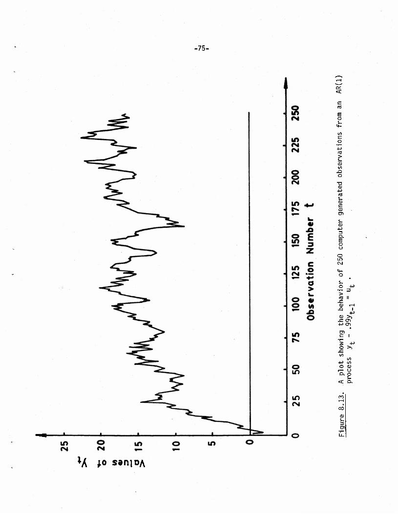
-75-
en <c
c (T3
E o s- 4-
10 c o
•1—
+•> «3 > S_ <u to
-Q O
•o a>
+-> 03 s- <u c <1> CT>
%- <u
+-> 3 D. E o o o Lf) CM
<4- O • s- o +J •^ 3 > (0 II -E aj i—l .a 1
-l-> CO >1 -E <y> +-> CO • CD c 1 • ^ 2 +-> o >)
-C </>
l/l +-> V) o aj
r— o Q- O
S- < Q.
00
co 5- 3
*A *o s9nioA

-76-
O s- 4-
A
to --—•* £ -C O ^•M' •n-
S- -t->
> £ s- o cu
"r— to +j _Q . O o £ Cn 3T3 01 4- cu •
£ re O S- II
cu 4J E i- f0 CD QQ.
r— CD 0)
r^ 1. S- JE o %- cu +->
00 o 4-> •!- o 3 2
<D o Q. r— 4-> £ </) -Q 3 o </>
CO «3 c_> cu 1— u
-a o o aim s- +iN a fO E £ •^ c-^
4-> 1—1
to -o ai cu cu
to «=C <u (Ö .£ .a 4-> £
fO 4- A
o o LO
to m
cu • 3 •
o II
C\J o CO I-»
CO cn CM o
Ln co o
I—1 r—1
CO «3- CO
CM 1-H CO CO
CO o CO cn
>3-
CO o
•
O 1-H
i-H OJ CM
CM CO Ln
CO t-H CO oo o •
cn LO t-H
CM CM CO •=3-
co
1-H CO
^1-
cr> o •
CO cn to O
CM CO CO •
CO CO
1-H CO co
CM i-H
r~« co cn I—1 co •
CM CO
o CO •
Ln <3-
CO 1-H
e
CO O CO
r-H Ln CO •
I-H CO
o CO
Ln i-H •
LO e
i—i
CO CO o
CO o CO
CO ^1-
1-H
«3- CT> 1^-. CO
1-H
CO CO cn
CM o CO •
CM *3-
cn 1-H •
CO 00 Lf) i-H
cn CO CO
CM o CO
I—1 o CM
OJ cn CO T—1
o CM
o CO •
o «3-
CO CM
r—1 LO cn CO
i-H
CO CO CM
cn CM cn
CO
Ln CM
o I-H CM t—1
Ln Ln CM
CO CM 00
CO CM
CD fO _J
-£
S-
4- O
CU 3
<0 > CD fO _l
.£
s-
4- O
CU 3
(8 >
.£
CD (0 _l
.£
4- o
cu 3
r— A3 >
JE
CD
—1
s-
4- o
cu 3
r— re >•

-77-
th e estimated autocorrelation function, for h=0,1,...,50, and in
Figure 8.14 we show a plot of r(h) versus h . As is to be expected,
this plot conspicuously shows the slow, and almost linear decay, of the
estimated autocorrelation function.
Since the estimated autocorrelation function of the generated
series decays slowly and linearly, we consider wt=yt+l~yt ' t = l»2»
..., the first difference of the generated series, and investigate the
behavior of its estimated autocorrelation function. Recall, that if
8, were to be exactly equal to -1 , then the w.'s would be described
by an innovation process whose autocorrelations at all lags other than
0 , is zero.
In Figure 8.15, we show a plot of the time series generated by the
w.'s , for t = 1,2 249. In contrast to Figure 8.13, we see that the
differenced series {wf} reveals fluctuations around a fixed mean of
zero. In Table 8.8 we give values of r(h) , the estimated autocorrela-
tion function of the w. series, for h =0,1,...,25, and in Figure
8.16 we show a plot of r(h) versus h . We contrast this plot in
Figure 8.16 with that of Figure 8.14, and note that in the former, as is
to be expected, the autocorrelations at lags other than 0 are, barring
sampling variability, effectively zero.
8.9.2 The Covariance Function of Some Processes with an
Underlying Trend
As a note of caution, it is not true that the tendency of the
estimated autocorrelation function to decrease slowly necessarily
implies that a root close to 1 exists. Such a tendency can also be
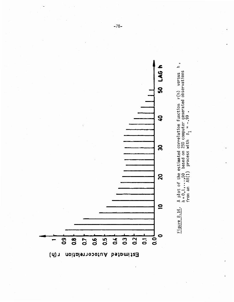
^78-
I
x X X
Q
S
01 to E 3 O Ul •!- S- 4->
> > s- O)
-—» «1 -e ja — o
S_ -o
o <e •r- S_ •4-> 0) • O C C (UOi 3 TOOT
I
1)
O
s-
O -M •r- 3 +•> Q. T- <o E ca
i— O <U O s- x: S- O 4-> O LO •!- UN 5
to tu o o S- n.
O
cu o -M rO -a E 0) •I- to -I-5 nj to .Q at
<U O .-I -E LO — +•> «a:
'< 4- . O •
•PH I« o «
°- ii g
co
oi
O G» O* Ö Ö OO O O O
(q)j uoijo]ajjooo;nv P^lDaijjsg

•79-
o m <N <N *- — o o — «- I I I
•^ jo sanjDA *N CM
I I O
s_ CO
-4-> 3 Q. E o o • o Lf> CJ1 CM CT> <U 1
-C •u II
H- ,_ O ca
CO cu .c o +-> c "r— cu 2 s- 01 to q- to 4- cu •^ o •o o
s- +J Q. to j-
•r-
4- i—1
o> cc: -c <: +-> 4- £ o fO
s- E o O •r- s- > 4- «3 .e to
CD e JD o • ^ CU 4->
J= fO 4J >
S- CTl CU C to •^ JO 3 o o .c -a to cu
4-> -p (O o S- ^~ GJ Q. . C
CU «=c en
CO
cu s-
oil

-80-
CO E o
•r— -M <T3 > S- <U CO -O O
T3 O)
„+-> A3
--» S- -£= cu
•— e: s_ cu
CD
sz s_ o aiffi •i- +-> en +-> 3 • u CX 1 = E 3 O II 1- O
c o cQ- o in •i- CM +•> .c (0 cu +->
r— J= •!- 0) 4-> 2 S-
00 S_ 4_ CO • O O CO CO o cu
O CO O CU +J <u o
r^ 3 O S- -Q (0 E Q. (O (L>
1— •o S_ CU CU"—•
-l-> 4- r-4 «a 4-«^ E ••- a: •r"0< +J CO +J cu co E
S- 03 CU -r-
JE 4- E +J o
cu s_ 4- J= q_ o +J
CO s_ cu o 3 tt-
r>— (tS > «
LO CM
o II
CM i—1
oo o
i
in CM
i-H
t—1 i—t
cr> o
i CNi
CO o •
o r—1 oo
o • CO CM
CO o
cn CO o
1
CM CM
CO o •
CO 1—1
1
«—1
CM
f—1 o •
r-> 1—1
o • 1
O CM
1—1
o • 1
CO CO o cn o
CO o r-l 00
i—i
CO o
«* o i—i
CM o •
i
co CO o
1
CO i-H
l-H O
CM cr> o •
i
in i—i
CO o
1
i-H CM O
1—(
o •
O i—1 CO
I—I
in o
•
Lag
h
-E
s_
4- o
cu 3
;>
.E
CD (0 _J
-E
S-
4- O
CU 3
«3 >

-81-
1
in
^-t1
<
c*
to 3 10
Is > CM
to to 0) o
e5 o S- a.
*- <+- o i—t
func
tion
fere
nces ^«^
o£
to
c4- E o °-5 S-
<° to to
rrel
fir:
E O
8« 03 >
•o-^ S- cu to
O E
'"^Ln -a •^CSJ <u • 5f « 4-> OJ . re ai
S- CTi <u : 0) •
C 1 +*^T cu
D) II
'S« S- r- II cu ca
s-= 4-> 3
r— Q-J= Q- , E +J
O T- < -= o 2
m tO
CO
s- CD
* -*—•
(q)j uoipidjjooojnv pajouuiisg
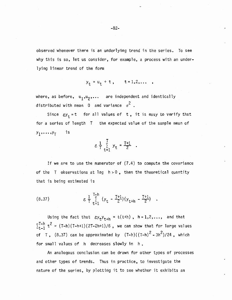
-82-
observed whenever there is an underlying trend in the series. To see
why this is so, let us consider, for example, a process with an under-
lying linear trend of the form
yt = ut + t , t = 1,2,... ,
where, as before, u,,u2»... are independent and identically
2 distributed with mean 0 and variance a .
Since ey. =t for all values of t , it is easy to verify that
for a series of length T the expected value of the sample mean of
yls...,yT is
T T+l 1 t=l z
If we are to use the numerator of (7.4) to compute the covariance
of the T observations at lag h>0 , then the theoretical quantity
that is being estimated is
(8.37) e^Y(yt.•)(yt+h.•,
Using the fact that ßy+yf+h = t(t+h) , h =1,2,..., and that
^t-1 t2 = (T-h)(T-n+1)(2T-2h+1)/6 » we can show that for lar9e values
of T, (8.37) can be approximated by (T-h)((T-h)2 - 3h2)/24 , which
for small values of h decreases slowly in h .
An analogous conclusion can be drawn for other types of processes
and other types of trends. Thus in practice, to investigate the
nature of the series, by plotting it to see whether it exhibits an

-83-
underlying trend. If the underlying trend appears to be a polynomial,
then, as discussed in Section 3.3, such a trend can be eliminated by
taking an appropriate number of differences of the series.
We have thus seen that the differencing of an observed series may
be motivated by two distinct considerations. The first enables us to
model certain types of nonstationary sequence of random variables, via
the mechanism of a integrated autoregressive processes, whereas the
second enables us to eliminate the presence of an underlying polynomial
trend in a series.
To illustrate the effects of a linear trend on the estimated auto-
correlation function of a series, we generate on the computer, 250
observations from an autoregressive process of order 1 with ß, =-.5 ,
and for which a linear trend term is added. Note that this is the
same series considered in Sections 8.3.2 and 8.5.2, except that the
inclusion of a linear trend term makes the generated series nonstationary.
In Table 8.9 we give r(h) , the values of the estimated autocorre-
lation function, for h=0,1,...,25, for the 250 computer generated
observations described above. In Figure 8.17, we plot r(h) versus h.
This plot clearly shows the very slow decay of the estimated autocorrela-
tion function. The estimated autocorrelation and partial autocorrelation
functions of the first difference of this series will reveal a behavior
analogous to those of Figures 8.6 and 8.9, since by differencing the
series we would have eliminated the linear trend.
An example of some real life data with a trend, and for which the
estimated autocorrelation function decreases linearly and slowly is
given in the next section.

-84-
CO
<u
"3
to +J
E •n- O i. o
»» (*_ 4J
.--» CO T5 J= S= CU *w o -o
s_ •^ -o •4-> to to
E > E O s- S-
•i— 0) O) •iJ en -l-s O -Q C O T3 3 c
M- XJ aj <L) s-
C 4-> 4-> O to •^ S- S- +•> <U fO to c tt)
I— OJ c 0) en •r-
S- ^— s- s- o OJ to o +J o 3 T3
+-> Q. C 3 F to to O
O TJ LO <u o . +J in 1 to F
CM II •r— s= T—
4J o ca (/I cu -o
CD J= <U CO +J .E f0 •^ 4J _Q s M- CO O #\ CO
Ln Cl) CO CM o 0) *t o 3 • s-
i— • Q. to
CM i-H
o LO Ln
CM Ln <3-
t—1 i—1
CM in CM
O 1-H LO CM
i^. •3-
en Ln CM CM
LO
CO CO LO
i-H CM .4
6 r-~
CO in .
O CM <5f
CO i—1
CO
•
in CO in .
00 i-H
LO "=3"
>ü- I-H
i—i
oo LO LO •
LO I-H
CO «3-
CM .72 Ln
r-H cn
I-H CM CO •vi-
I-H
o in •
o 1—1 OO t-H
CO Ln
CD to _l
S-
4- O
O) 3
r—
> Lag
h
Val
ue o
f r(
h)
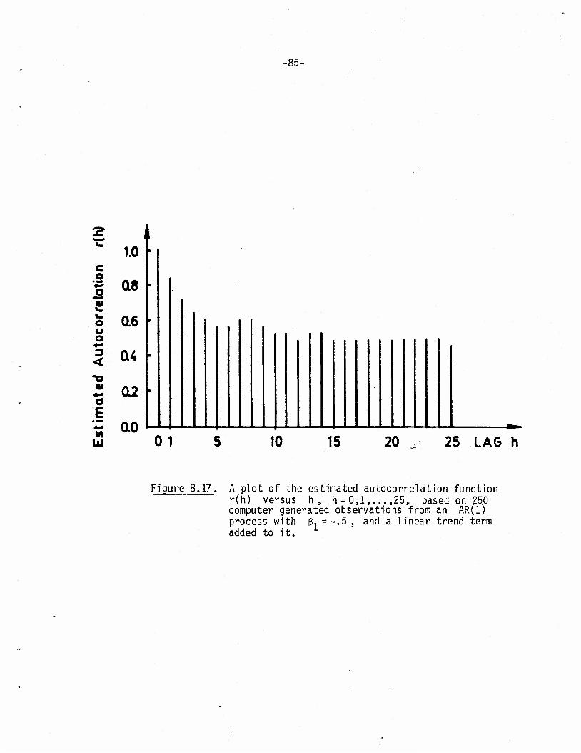
-85-
C O
o u o
•o
a 6 (A
LÜ
1.0 f
Q8
0.6
04
02
0.0 01 10 15 20 25 LAG h
Figure 8.17. A plot of the estimated autocorrelation function r(h) versus h, h = 0,1 25, based on 250 computer generated observations from an AR(1) process with added to it.
51 = -.5 , and a linear trend term

-86-
8.9.3 Behavior of the Estimated Autocorrelation Function of a
Real Life Nonstationary Time Series
In Figure 8.18, we show a plot of G. , the US gross national
product (GNP) in billions of US dollars, for the years t=1920 through
t=1979 (Source: Bureau of Economic Analysis, U.S. Department of
Commerce, Washington, D.C.). This plot indicates that the GNP series
is a nonstationary one, it being increasing (approximately) exponentially
over time. Thus it appears reasonable to first take the natural loga-
rithms of the GNP, InG. . A plot of y. =1nG. x1000 versus t is
shown in Figure 8.19; the actual values of y. are given in Table 8.10.
Figure 8.19 shows that the yf series is also not stationary, it being
increasing (approximately) linearly in t . The estimated autocorrela-
tion function of the y. series, for lags 0 through 20 , is shown in
Figure 8.20. Because this estimated autocorrelation function decreases
linearly and slowly, we consider the first differences of the y. series,
w. =Ay. =y.+, -y. , t = 1,2,...,59 . A plot of w. versus t is shown
in Figure 8.21; the actual values of w. are also given in Table 8.i0.
From Figure 8.21 we see that whereas the w. series appears to have a
constant level (mean), its fluctuations in the earlier years, 1920-1947,
appear to be more erratic than the fluctuations in the latter years,
1947-1979. A possible explanation for this behavior is that "automatic
stabilizers" such as unemployment insurance, workmens compensation, etc.,
which were introduced into the economy as of 1947, tend to make the GNP
less erratic. Plots of the estimated autocorrelation and partial auto-
correlation functions of the w. series are shown in Figures 8.22 and
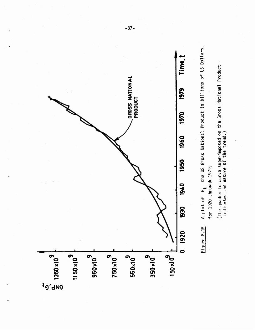
-87-
E
91
9»
S
o 9t
o 2
Ok
lO S- (O
o Q
4J t/1 O ^5 3
•a M- o O
Q- l/l E r— o 03
"1— E 1— o ^~ •1— •1— +-> -Q
c •p~ to
to +J o CJ £_ 3 O
•o o CJ 5- r~
Q. •P
,_ E--—• (O o • E -o o T3 E
•1— at cu +J </) i- (O O +J z
E CJ 10 •i- .E c/1 i. 4-> O CJ 5- cm-
CJ3 3 o • to to cyi CJ =3 r^ CJ s_
CD > 3 0) i—i S- +J .E 3 (O +-> CJ E
3 O CJ 4-> O •r- -E
o s- •)-> -t-> -E (0 -p S_ CO
M- -O CJ O o to +->
CM 3 res +-> CT> cr CJ O f-H •r—
r— CJ -o Q. S- -E E
o 1— T- <C 4- —
CO
CO
CJ S- 3
-L X o> a>
©
s o x" o in
9» o ^< o in a*
a» o ••• X
8
J-
OV a»
o m in
o *x o in o
o» o *x
\ 9'dN9

-88-
o o o © o o o o O a* m ^~ ^» 10 \o \D
© o in
© o tf>
+J to o to 3 o
T3 s_ O • CD S_ tn a. r- CU
CTi .E ^— i—i +j<—. 03 • E .c <t- -O O CT> O E
•i— 3 ai •IJ O £ s- n3 s- -E 4-> Z _E •1-5
-t-> •r- CO to s- JZ 1/1 o <o -P O CM C7> S- CTi O 4-
CD .—1 i— o
0) S- <D <D .E o -E s_ 4-> 1- +-> 3
4-> 4- E «3 O o
o O E
e o -a cu .E I—1 CÜ -E 4-> CO 4-> •r— CO o s- a> Q. to (0 £ £ <u CD °r— ••- +J O +-> S- A3
P= CD U to CLT-
r— S- 3 -D ro ta tO E S- r— •i—
3 t— CU +J o E +J (Ö Q •r- O E i— 3
t/1 -a cu =J 4-> o .E JZ s- +-> M- cno.
O »(— <+- (0 i— o to S- ns
e +-> E +-> o tO O o •I— •r— ^— 1— 0) +J a. 1— -E ns
°r- I— z: < -O •—-
CT)
co eg s- 3 CD
*9 ui*000l

•89-
>> «t
o 4- o O o .—1 <U
X
4-> a) o s- 3 <u -a 4- o 4- S- •^
Q_ T3
,_ -a (O s- c (0 o s
•r• s- +-> o (8 4- Z
-t-> to in to 5- o •r— 5- 4-
CD (1)
CD .£= .e +J
o -u r-H • 4- 00 O -f->
>> <v E 1
r— J= I—1 -Q •P + fO •r- -P
1— s- >> en II
o -t-> 3
, <a -a s- £= 3 (0
+-> <0 CT) c 1^
CTi <D »—I .E +•>
«N 3 o
4-> S- >>
4- o o CM
cr> CO rH
3 II
1^ +-> <T3 >
s- o q-
o
aj s- CÜ 4- 4-
+-> to S-
>> I
>> II
3
4-> CD
O O o
o c aj s- cu 4- 4-
to
I 1—1 +
II +->
-p CD c
o o o
s-
CM ID cr> !—I CM to OO to LO H CO rl (Jl O ^f
O P». 00 r-~ co oo r>- CM
r--r-^cooO'si-i-«i-«.c\JcocM<d-iooC'--i r->. oo oo i—i to CM i—i i in CM CM in oo in
to oo ^1- en
CO CM t—l OO CD CM to i—I CM CM "vf-lOin0O«5l-^i-0O000Of-l
en r~^ ^- CM
CT) lO ^l" CM N w CTi n CM oo oo <3- to to to to
Öl «3- trs CO i—i CT) I—1 00 o CM CM 1^. "vf "=1- in m in in to to to to to to
CM r-«. CO CM O CM 00 CM to to to r*» to to to to
o m cr>
.—I CM 00 in in in ai ro ei
* w u in m in tn cfi en
in CTl
oo m CTl
en in CTl
o to CTl
<-l CM CO to to to CTl en en
CM CM CM CM CM CC O ^f
C0 CO
co to «3- o
CT) to =3-
CM I co m
o to
to t—1
00 in
in CO
r-» to
00 I—1
•si- te o
1—4
o 00
o to I—1
1
00
1
to CO
CO io
co in CM CM
CO CO
to m CM to co <- <3- m o i—i <—i CTI co CM «si- m in in m in m in in in
«tf- co en CTl CO m o CO t—1 o to CM t—i in CM in
CM l-H to t—i r~- to to r» in in in in i—i CO I-- in to to to r^ to LO CO oo in in m in m in LO u->
O i—l CM CO CM CM CM CM CTl CTl CTl CTl
«st- tn to I-«. CO CTl o t—1 CM oo CM CM CM CM CM CM oo CO CO CO CTl Ol CTl CTl CTl CTl CTl Ol Ol CTl
o CT)
CJ CD rö O.
c o
-o
c o o
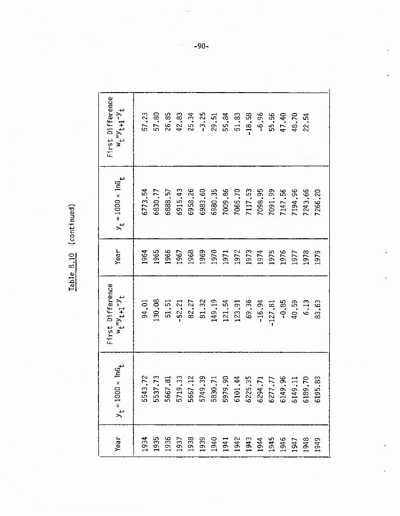
•90-
c o o
CO
ra I—
0) (J c <U +J &- >> CO o LO CO "* LO »—i <d- CO CO to to o o •vi- a) 1 CM CO 00 CO co CM LO CO CO LO en LO «d- r- LO M- i-H <4- + f» r-. LO CM LO CO en LO i—i CO to LO r-«. 00 CM •r- +-> LO LO CM «=*• CM i CM LO LO 1—1
1 i LO *3- «* CM
II
W s s- •l_
u.
+J es E i—• ^1" !*«. r-» co «3 o LO to O co LO en to to to o X LO i->- LO ^j. CM tO CO 00 r-~. LO en en LO en to CM
o CO o 00 LO 00 CO o en LO r-. CO i—i r-» «3- CO to o r-> co CO 1—4 LO CO 00 o to i—t en en «3- en «3- to o r< 00 CO CTi en en en o o i—i o o 1—4 i—i CM CM I—4
II
•U
to to tO to tO to to r-> r«. i-^ r-. i-v. 1*» r~- r~- r~-
>>
s_ <d- LO tO r~- CO en o I—4 CM co •* LO to r~v CO en 03 tO tO tO «3 tO to t»-. r«. r~- r-. f-v. [--. r-». r-. 1^. r-. O) en C51 en en en en en en en en en en en en en en >- i—< <—4 1—1 1—1 i—i t—i 1—4 i—i t—4 I—I »—I 1—4 «—) t—i 1—4 i—i
QJ O E 0) +->
£- ^ i—i 00 1—4 r—1 r-~ CM en •vf t—i to *=f i—< LO en CO CO 0) 1 o o LO CM CM CO i—i LO en CO cn CO CO LO 1—4 to M- r-l 4- +
**• o 1—4 CM CM T—1 en i—t CO en to r-~. o o to CO •r- 4-> en CO LO LO co CO «3- CM CM to i—i CM 1
•<* CO
II 4J 4->
r—4 1 1—4 1—4 i—i i i—i i
c/i 2 i. •r— U_
+-» C5 c •—• CM co 1—4 CO CM en i—l o >* LO i-H r-. to i—i o CO X r-- r-* CO CO 1—4 CO r^. en «d- CO r~» r-. en i—< pv. co o CO r~* r-». Ol r~- en o en i—i LO "vf r-. en en en LO o *3- CO tO I—1 to «3- CO i-*» o CM en r-. v± >vt CO en o LO LO tO r-«. to r-- CO en i—i CM CM CM 1—4 1—4 1—1 i—i I—4
II
LO LO LO LO LO LO LO LO to to to to to to to to
>>
S- ' *3- LO to r*. CO en o !-H CM CO vj- LO to 1»-. CO en «3 CO CO CO CO CO CO «d- «vt -* <- >* «3- •* "=3- v3- •vi- a> en CTl en en en en en en en en en en en en en en >-
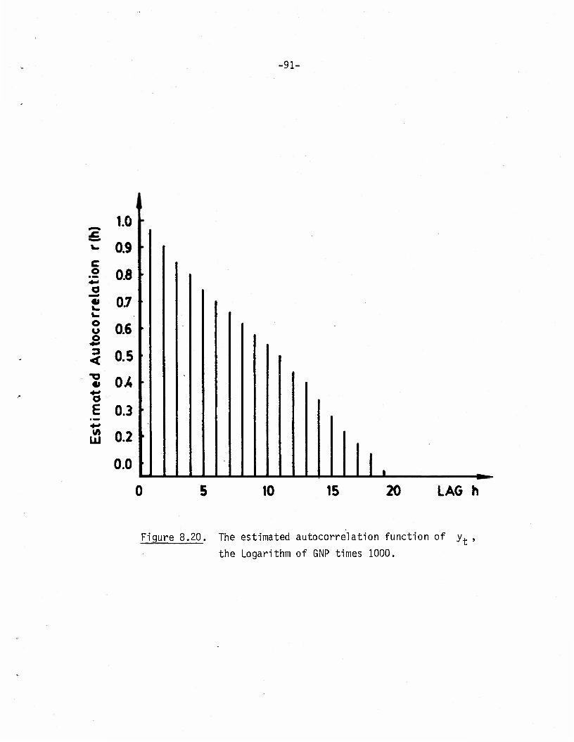
-91-
C o
"31 o u o
'S E
LU
1 1.0 •
0.9 •
0.6
0.7
0.6
0.5
0M
0.3
0.2
0.0 -^»
10 15 20 LAG h
Figure 8.20. The estimated autocorrelation function of y
the Logarithm of GNP times 1000. t '

-92-
</1 3 to
4-* S- a»
«f >
E *
o o
P" o I—1
X
3 2T CJ3
O» c *«~ r—
M- O
8 a) o c
0» <L> ^a s-
cu M- 4- • (— •
S -a <n
OJ </> i—i s-
•r- J= H- en
3 0) O -c s-
s? Ot o ^•* 4-> CM
3 cn t—i
<4- S-
o o o ««* +J
«2 O i— 0) Q. E
•I--
< -U
s i—1 CM a» oo
cu s- 3
8 CD
OS Ll_
o o o o o o o o o o <n 10 ot <N <o I I I I I
•93-
8.23, respectively. In contrast to Figure 8.19, we note from Figure
8.22 that the autocorrelation function at lag 1 is significantly
different from 0 and takes smaller values for the other lags. How-
ever, it is difficult for us to claim in Figure 8.22, a pattern of
either an exponential or a sinusoidal decay. A similar type difficulty
is apparent in Figure 8.23. Thus it appears that the w. series
cannot be reasonably well described by an autoregressive process of the
type discussed here; more complicated models to be presented later on,
may be necessary for analyzing this data. Our main goal here, is to
show Figure 8.20.
8.10 Forecasting (Prediction) for Stationary Autoregressive
Processes
Suppose that a sequence of random variables {y.} , t = l,2,...,
can be described by an autoregressive process of order p
yt + ßlyt-l + ß2yt-2 + '*' + ßpyt-p = ut ' t = P+1' P+2"--> •
Let yt_i> yt-2"*" be tne observed values of the random variables
^t-1' yt-2"*" * 0ur goal in this sectl'on is t0 determine a
procedure «which would give us a best, in the sense of minimum mean
square error, forecast (predictor) of the unobserved variable y. .
We shall soon see that if the roots of the associated polynomial equa-
P tion 1 3 xP~r = 0 of the AR(p) process given above are all less
r=0 r
than 1 in absolute value, then the best predictor of y. is indeed
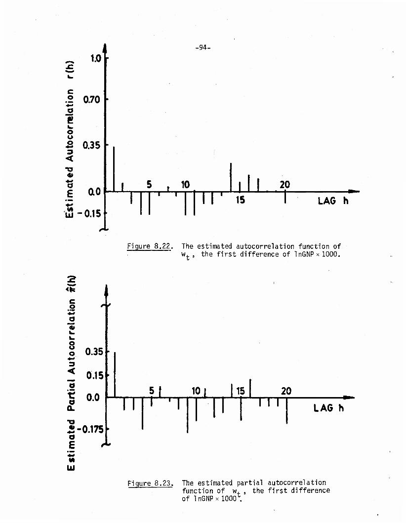
-94-
^ 10
.1 0.70
Ü o
I 0.35 3 <
4»
E ao 10
UJ-0.15 n d 20
15 LAG h
Figure 8.22. The estimated autocorrelation function of w+ , the first difference of InGNPxlOOO.
<*! I
4»
8 o
<
"5 XL o Q.
0.35
0.15 •
0.0 n Z -0.175 o E «ft
LU
It r^r Si 15 20 TTT LAG h
Figure 8.23. The estimated partial autocorrelation function of w. , the first difference of 1nGNP x1000 .

-95-
the natural quantity
~hh-i - Vt-2 - • • • - V t-P •
To see that the above is true, we first note that under the condi-
tions of Theorem 8.1 in the equation
yt = -ßiyt-i-32yt-2'---- Vt-P + Ut
u. is independent of y, -, y, «,... . Thus, the conditional expec-
tation of yt given that yt_1 = yt_1» Yt_2 = ^t-2 ' ' " is
e(ytlyt-l=yt-l' h-Z^t-Z""^ = "3lyt-l " ß2yt-2-"--Vt-p ;
the right-hand side of the above equation can be used to forecast y. * *
t-1' yt-2! given y. ., y. 9,..., * *
Now let f(yt_1,yt_?,...,) be any other function of the previous * * * *
values yt_i» yt_o»'«'> and suppose that we use f(y. ,, yt_2"">)
as a another forecast of y. . Then the mean square error of f(yt_i»
yt-2"" ' as a Prec'ictor of y. is
£[f(y*_1,...)-yt]2=e[f(y*_1,...)+31y*t.1+...+ßpy*t.p-ut]
2
= £u2+e[f(y*t_1,...)+ß1y*.1+...+ßpy*t_p]2 .
since u. is independent of y. ,, yt_?»...
The above is minimized when f(y+_i» yt-2'"*^ = ~ßlyt-l " e2yt-2
•••-Vt-p •

-96-
In general, when the conditions of Theorem 8.1 are satisifed, the
best (minimum mean square error) forecast of y. given y+_s_i»
yt-s-2'"" ^s-0^ 1s £(yt'yt-s-r yt-s-2""^' the conditiona1
expectation of yt given yt_s_1« yt_s_2>--" where £{^tlyt-s-l'
yt-s-2"-- } = aslyt-s-l + as2yt-s-2 + "• + aspyt-s-p ' and asl =
a ,,...,a = a are given in equation (8.6).
8.11 Examples of Some Real Life Time Series Described by
Autoregressive Processes
In this section our aim is to demonstrate the methods of the pre-
vious sections by considering some real life data which can be reason-
ably well described by autoregressive processes. It is entirely
possible that the data can also be described by some of the other models
introduced later on. However, at this point in time, it is convenient
to introduce the data and use these to indicate the practical usefulness
of autoregressive processes of a simple order.
8.11.1 The Weekly Rotary Rigs in Use Data
A rotary rig is composed of five major components and costs
upward of $500,000 each. It is used for drilling for oil and gas. The
number of rotary rigs in use per week, by state, is an important compo-
nent used in econometric models of the oil and gas industry. Such
econometric models are of interest to the U.S. Department of Energy.
*This data and its description was given to us by Mrs. B. Volpe, Energy Information Office, U.S. Department of Energy, Washington, D.C. It has been abstracted from a Hughes Tool Company, Houston, Texas, report, entitled "Average Number of Rotary Rigs Running - by State."

•97-
In Table 8.11, we give 82 values of the weekly number of rotary
rigs in use in the Southern Louisiana Inland Waterways, from the period
starting December 10, 1979. A time series plot of this data is shown in
Figure 8.24. An informal inspection of this plot reveals that the neigh-
boring observations tend to behave similarly, suggesting a positive
correlation between them. This is in contrast to neighboring values
alternating in sign implying a negative correlation between them. There
does not appear to be a well discernable underlying trend in this data,
nor does the data reveal any systematic fluctuations indicative of an
underlying periodicity.
In Tables 8.12 and 8.13, we give values of the estimated autocorre-
lations and partial autocorrelations of this data for lags 1,2,...,25.
In Figures 8.25 and 8.26, we show plots of the estimated autocorrelation
function and partial autocorrelation function, respectively. The
estimated autocorrelation function appears to decay exponentially, and the
estimated partial autocorrelation function shows a value which is signi-
ficantly differently from zero at lag 1 only. These plots suggest that
the data of Table 8.11 may be reasonably well described by an autoregres-
sive process of order 1.
An estimate of the autoregressive parameter ß, can be obtained by
using the estimate r(l) = .722 in (8.28). The estimate r(l) is
consistent with our observation that the neighboring values in Figure 8.24
tend to behave similarly.
Based upon the above, a proposed linear stochastic model for the
weekly number of rotary rigs in use in Southern Louisiana Inland Waterways

-98-
Table 8.11
Values of the Weekly Rotary Rigs in Use in The Southern Louisiana Inland Waterways for the
period starting December 10, 1979
Week Number
Rigs In Use
Week Number
Rigs In Use
Week Number
Rigs In Use
Week Number
Rigs In Use
1 74 21 75 41 75 61 81
2 79 22 84 42 80 62 79
3 82 23 83 43 78 63 75
4 83 24 76 44 79 64 77
5 84 25 80 45 81 65 11
6 79 26 79 46 82 66 79
7 80 27 74 47 80 67 87
8 78 28 73 48 79 68 88
9 75 29 70 49 73 69 87
10 72 30 70 50 75 70 90
11 73 31 68 51 76 71 99
12 74 32 68 52 78 72 88
13 77 33 74 53 81 73 84
14 84 34 68 54 79 74 79
15 81 35 73 55 83 75 82
16 77 36 72 56 82 76 84
17 76 37 74 57 81 77 81
18 72 38 74 58 77 78 75
19 77 39 79 59 75 79 83
20 73 40 81 60 74 80
81
84
84
82 81
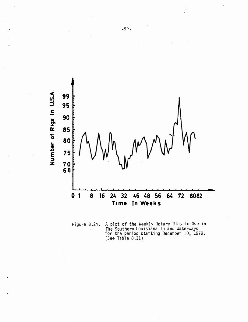
.gg.
i < 99 3 95 c
V) 90 o»
ÜC 85 ^_ o
80 «I
E 75 3 z 70
68
0 1 8 16 24 32 46 48 56 64 72 8082 Tim« In Weeks
Figure 8.24. A plot of the Weekly Rotary Rigs in Use in The Southern Louisiana Inland Waterways for the Deriod starting December 10, 1979. (See Table 8.11)

•100-
o->
00 «1
<u ^"^*f—• JC X! (Q
S- 1—
M- C O O
•i— (O +J 4-> O (0 c -a 3
<4_ CU CO
C ID O •r- E -P -i- (6
r— CO CM CU C7! I-H S- T- • s- a: CO o
o >, CM O >—
r— +J -Ü -Q 3 0) (W re a;
1— 3S T3 <D <u +J J= (Ö -t-> E
•r- q- 4-> O CO CU «\ CU IT)
-C CM +j «>
CO i—l
5 11 to
o
in CM O
C\J 1—1
in o CM
ro O
t—1 I—1
I-H I-H
oo CM
«3- o
o 1—1
«3 1—1 •
CM CM
o o •
CTl 00 t—1 1—1
CM
o o
00 CNJ i—l o
CM
CO o
r»^ o CT> i—l o
to t—i 1—4 00
1—1
CO o
m 00 I—1 • «—1
C7> O
•=3- CO CM •
CO i—I
co o •
oo <=i- 1—1
CO o
CM CM «a-
t—1 O
I—1 CM
i—l
"3" O
en (0 _l
'S" s-
4- O
CU
>
xz
en rO _i
s-
Cl-
O
CU
to >
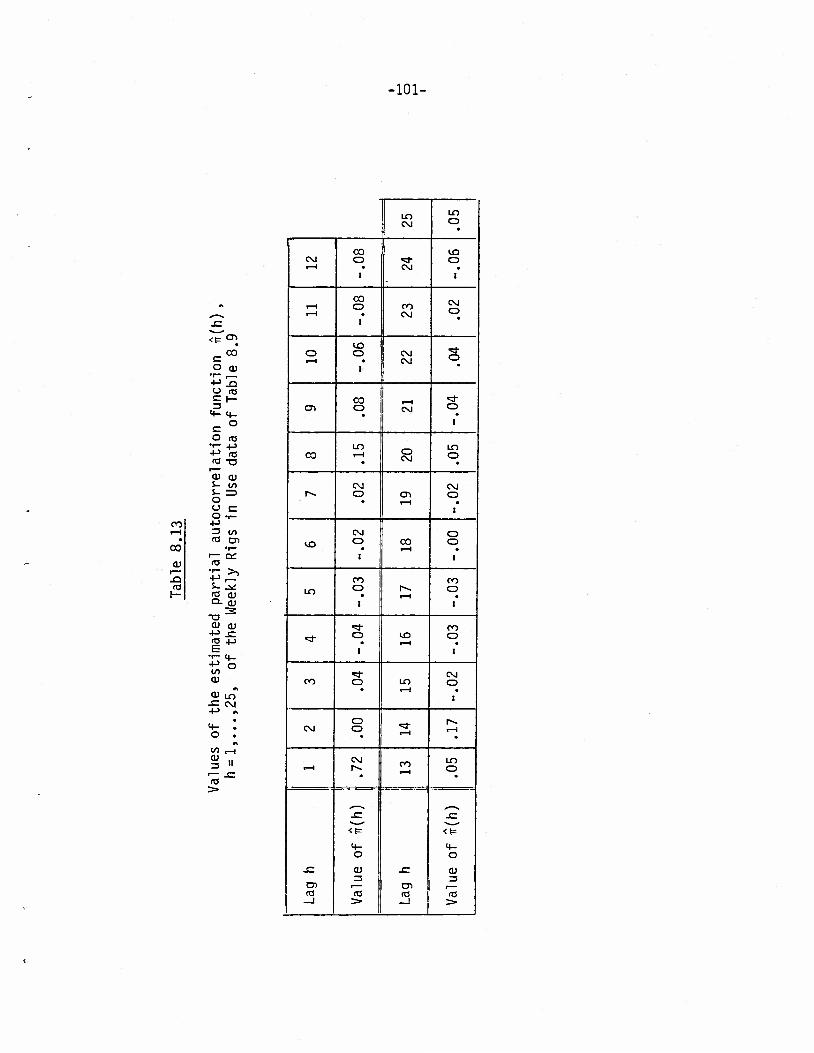
•101-
<t= °l 00 c
O CU •l— r—
••-» ja O (6 5= 1— 3 4- q_
O C O re •I- +J -f-3 <0 ro -o
r— cu cu i- V) S- =) o o c: O T-
CO +j I—1 3 m • * CD CO •r-
«— DC cu fO
1— •^ >">
-O -t-9 i— re S- J*
I— rO CU CL CU
3 -a cu cu
••-> J= re +J E
•i- 4_
•*-> O 01 cu
« CU LO -= CM +-> «
4- . O . «\ t/> ,-(
s» ro
LO CM o •
••
oo vo CM o "=3" o I—H
1 CM
1
r—1 CO o CO CM
o • .—1
'" CM
O to o CM o i-H •
1 CM
CO >3- CT> o CM o •
1
00 LO
• O CM
LO O •
CM CM r-» o CT) O
i—f •
CM o lO o 00 o «
1 r—1
1
CO CO o r-. o • i—i •
«3- CO <a- o • to
i-H o •
1
"5J- CM co o LO o
r—1 •
CM o o •
"3" t—1 I-H
r—1 CM r». CO LO
o *
JC .c v^^» **_^ <t= <t=
4- 4- O o
-C CU 3
_c cu 3
D1 r— en r— ro ro re <c _l > _j >
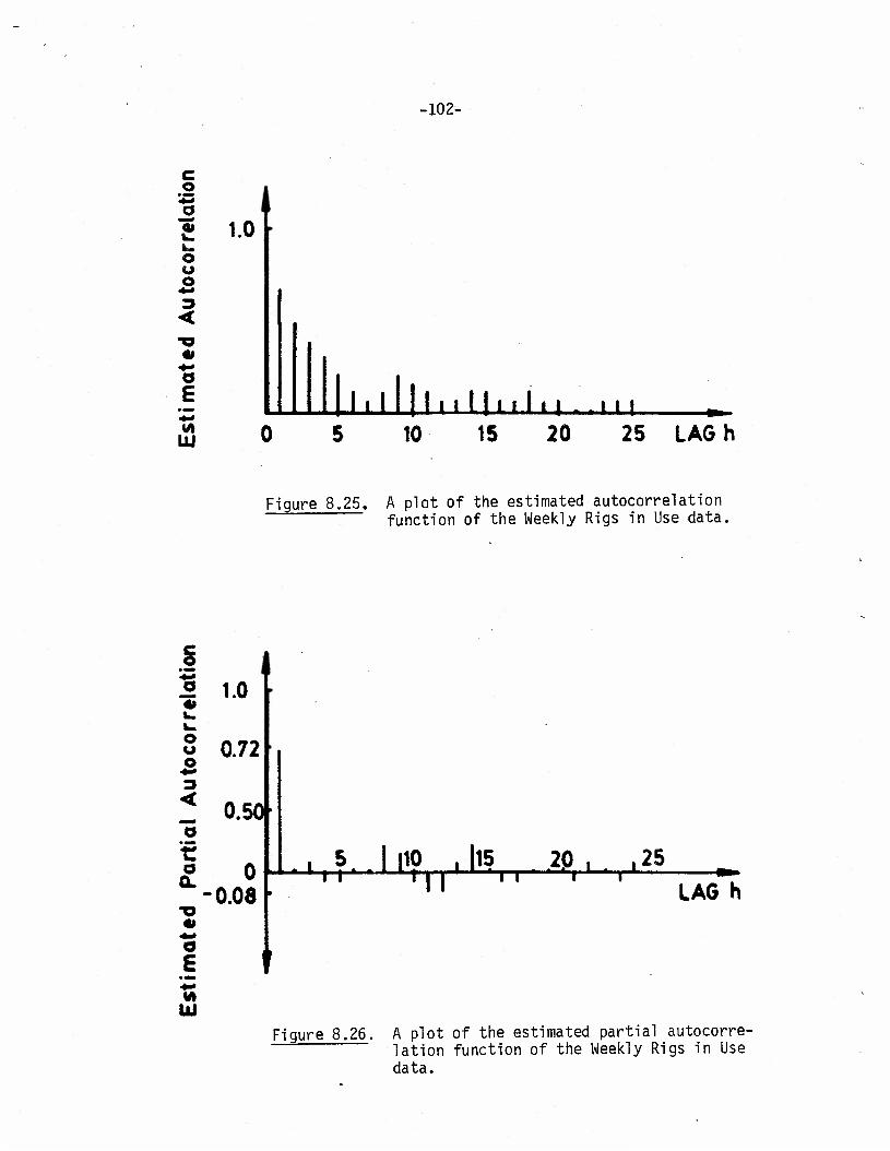
„2 £ 1.0 o o
•102-
O E ** Mi m
I. I I 11. . 111 i I . j .
10 15 20 U ^ 25 LAG h
Figure 8.25. A plot of the estimated autocorrelation ' function of the Weekly Rigs in Use data.
« im. mm
O u o *•»
<
"5 f o
OL
1.0
0.72
0.501
0 -0.08
© £ w
UJ
-u. TT 110 , 15
TT 20, 25
LAG h
Figure 8.26, A plot of the estimated partial autocorre- lation function of the Weekly Rigs in Use data.

•103-
y. is for t = 2, ...,82
(yt-78.5) = .722(yt_1-78.5)+Gt ,
where the LL'S , with
ut = (yt-78.5)-.722(yt_1-78.5) , t = 2 82 ,
are known as the residuals. The quantity 78.5 represents the mean of
the data.
In order to assess how well the proposed mdoel describes the data
of Table 8.11, we see if there is any recognizable pattern in the resid-
uals. If the model were adequate, then we would expect that as the
series length increases, the u.'s would become close to the innovations
u.'s . Thus a study of the u.'s would indicate the existence and
possibly the nature of model inadequacy. In particular, the behavior of
the estimated autocorrelation and partial autocorrelation of the u.'s
would yield valuable evidence about model inadequacy. The absence of a
recognizable pattern in a plot of these functions would give us some
assurance of model adequacy.
In Tables 8.14 and 8.15, we give values of the estimated autocorre-
lations and partial autocorrelations of the residuals in question for
lags 1 25 . In Figures 8.27 and 8.28, we show plots of the data in
Tables 8.14 and 8.15. Since these plots do not reveal any recognizable
pattern, we conclude the adequacy of the proposed model.

•104-
co
cu
10
<1>
o
o -c0
+^
3 **• re M- I—
o * o
(0 ? -•-> CJ ^ -o
O 'Z </> O 1«3
2 •§ = 5° in
T3 *" CD
15>, 4->
8 *
CO _VH-
3 II
« •=
CM i—1
*3- O
<—< i—1
CM o •
O i—I
o
CT! CM
CO i—i
o • O CM o
l~~
i—<
i—i o-> o o
«D «a- o •
1
CO I—) O
ID CO o l-v.
CM o 1
«=h CO o ^O
I—1
1—1 o •
1
00 o ID t-H
CO o 9
CM CM o
i I—1
CM I—1
r—1 o o •
CO CO o
i
CD
—1
S-
q- o cu 3
> CD (0
S_
4- O
<D 3
(O >•

• 105-
<t=
<D
= "2 O O i-H
•1- = 1—1
-t-> „r O «3 E ' ' 3H<1I
^ a: JQ
= «C «a o •-
!J3 =<4- 75 « ° a> E "3 2 p +J r s- « o <4--a
Lf> o «—I o W 0) • 4J 1 l/l 00 3 (O =>
(O = 0) -o c
r— r—" *'"" *"" _Q re "> fO ^ <U w H- +) S- Cl
S- -r~ re <» ^ Q.-C
•n >> "O •— 0J t- -^
4-> O <1> re a» E „2 4JO <U t/1 CM J= d) «+J
0) • S- J= • P +j «4-
c/1 a; 3
CM I-H
o i
I-H I-H
00 o
• • •
o r—1
o 1—1
C7t CM I-H •
00 I-H o o
CM
LO o
r^ CM i-H •
1 i—I
LO o •
to O
1
OO t—i
CM O
IX)
oo o •
1 I-H
I-H o •
1
•3- oo o
I-H
LO O
00 O LO i-H O •
CM CM o
1 i-H
o I-H
i-H o o 00
i-H
CM r—1
re
s- 4- o
3
re >
Oi re
s-
4- O
CU
re >
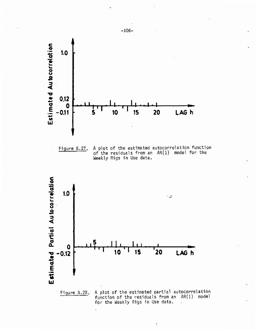
-106-
C o 1
« 1-0 o «
t_ o u s <
• 0.12 | 0 .E -0.11
UJ
JJ. r^ i •• i • i
10 15 20 LAG h
Figure 8.27. A plot of the estimated autocorrelation function of the residuals from an AR(1) model for the Weekly Rigs in Use data.
s • •mm
a * 1.0 o o s <
r a Q.
E
Ul
0 -0.12
l?,,.ll JJL 10 IS 20 LAß h
Figure 8.28. A plot of the estimated partial autocorrelation function of the residuals from an AR(1) model for the Weekly Rigs in Use data.
•107-
8.11.2 The Landsat 2 Satellite Data*
The Landsat 2 satellite is an earth orbiting satellite which
measures the amount of reflected energy in 4 bands of the electromag-
netic spectrum. The satellite travels from north to south over the
day side of the earth. As the satellite travels, an oscillating
mirror sweeps out a 150 kilometer long scan line in a west to east
direction. The mirror reflects the energy from the ground onto an
array of detectors on board the satellite. The reflected energy is
converted to an electrical impulse. Several such impulses are inte-
grated over a short period of time and then transmitted to the earth
via ground stations as discrete signals. The discrete signals
represent light intensities, 0 denoting black, and large values
such as 130 denoting bright.
In Table 8.16 we give 496 values of the light intensities
observed by such a satellite over a sand dune field in the Sahara
Desert. The measurements are indexed by the distance traveled by the
satellite (instead of time) and are recorded at every 80 meter
distance. Note that the entries in Table 8.16 are taken from a
computer output with an exponent notation; thus the first observation
.74000D + 02 denotes 74.000. The light intensities in this table
range from 0 to 127 . In Figure 8.29 we show a plot of the first
*This data and its description was given to us by Dr. Mark Labovitz of the National Aeronautics and Space Administration, at the Goddard Space Flight Center, Greenbelt, Maryland 20771.

-108-
Table 8.16
Values of the Light Intensities Observed by a Landsat 2 Satellite over the Sahara Desert
1- 3 t- 14
17- 24 25- 32 32- 40 41- 48 49- 56 57- 64 65- -in
73- 30 81 - 88 S9- 96 97- 104 105— 112 llj- ii.0
121- 122 12*- 136 1'37- 144 145- 152 153- 160 161- 168 169- 176 177- 184 185- 192 193- 200 201- ^*0F* 209- 216 "> . "7 — 22 <! 225- ':> -;' 2
233- 240 241- 248 249- **56 257- 264 265- >72 273- 280 281- 2i?w
3—';• — wwO _ ^ 7 — w 'J /
345- 3o*i
353- 360 jai- 36a 269 — 376 277- 3S'4 "i"85- 392 703- 400 -tOi- 4uS ^0'" - -*> 1 i 41/- 42* 423- 432 -33- 44 0 --ii. - -143
—r *r *; 45ö -~ i / • -r ö 4 4<is- 4/2 4/3- TÖÜ 48i- 4sa 4ÖV- '49o
0.740000+02 0.660000+02 0.86000D+02 0.S3Q00D+02 0.940000+02 0.950000+02 0.530000+02 0.380000+02 0.780000+02 0.105000+03 0.870000+02 0.105000+03 0.760001+02 0,770000+02 0.720'j...'ö-t-ö2 0.920000+02 0.9000ÖD+0i 0.870000+02 0.9600 00+02 0.3000015+02 0.920000+02 Ö.900000+02 0.790000+02 0.600000+02 0.6400011+02 0.370000+07. 0.740000+0.7. 0.6ri-00D+02 0.970000+02 0.620000+02 0.62000D+02 0.30Ö00D+02 0.330000+02 0.340000+02 0.610000+02 O.370000+02 0.97000D+-J2 ij.•;>•'; OOCil + 02 o^ooon+os 0.7300001-02 0.760003+02 0.630000+02 0.750000+02 0.780000+02 0.690000+02 0.660002+02 •J.910000+02 0.330ÜÜD+G2 O.T80000+02 0.5200CD+02 0.3ÜÖ00D+02 0 370000+02 0.710000+02 0.U10ÖD+C3 O.SSOCOB+02 0.9 00000+02 0.95000D+02 u.V3CO0U i02 Ü.üiOOOu+02 0.82CO0Ü+Ü2 0.c/aüöOD+02 O.ylOÖCü+02
.0.710000+02 0.630000+02 0.790000+02 0.78000D+02 O.lOlOOD+03 0.1Ö200D+03 0.700000+02 0.950000+02 0.770000+02 0.103000+03 0.860000+02 O.lOlOOTi-03 0.7'M)0!;j+"2 0.340000+02 0.630000+02 O.90OOOO+O2 ... . •":>00D+02 0,910000+02 0.950000+02 0.730000+02 0.390000+02 0 . 850'>OOT02 0.820000+02 0.640000+02 Ü.6700QD+02 r. .870000+02 0.690000+0? \!. 6S000L'-r02 ü.370000+02 0 .630000+02 0.590000+02 C.370000+02' 0.770002+02 0.830000+02 0.67000D+02 0.890000+02 .:••. ?~0000+02 0 - 101000+03 0.530000+02 O.106000+03 0.ÜÖ0Ö00+C2 0 - ^';OGOO+O2' •J.d3ö00D+Ö2 0.740000+02 0.630000+02 0.690000+02 0 • ~ .".^'ICTl-4-A—I
o.750000+02 0.910000+02 0.540000+02 0.300000+0? 0 ,830000+02 0.73-JO jD+02 0. 1050G0+03 0.900000+02 0.340000+02 0.840000+02 •j. ':-• £0000+02 O.iiiOOUO-s-^i 'j.'yiuuuutui 0.940001:+C2 Ü.S.3Ü00D+O2
0.740000+02 0.700000+02 0.75O0OD+02 0.860000+02 0.110000+03 0.101000+03 0.800000+02 0.99.0000+02 0.730000+02 0.100000+03 0.900000+02 0.900000+02 0.750000+02 0.760000+02 0_. 730000+02 0.890000+02 0.930000+02 0.910000+02 0. »60000+02 0.700000+02 O.S400ÖO+02 0.S60000+02 0.330000+02 0.720000+02 0.730000+02 0.900000+02 0.780000+02 0.690000+02 0.390000+02 0.590000+02 0.560000+02 0-710000+02 0.710000+02 0.820Ö0D+02 0.790000+02 0.S30C0Ü+02 0.920000+02 0.990000f02 0,930000+02 0.108000+03 0.730000+02 0..710000+02 0.810000+02 0.650000+02 0.690000+02 0.710000+02 0.100000+03 0.730000+02 0.340000+02 0.610000+02 0.830000t02 0-390000+02 0.910000+02 0.950000+02 0.960000+02 0.320000+02 0.790000+02 0.920000+02 0.910000+02 0.38000Ü+C2 0.9SOOÖÜ+0* 0.840000+02
0.740000+02 0.860000+02 0.71OOO0+02I 0.93000D+02 0.11100D+03 0.35000D+02 0.780000+02 0.570000+02 0.750000+02 0.100000+03 0.101000+03 0.790000+02 0.330000+02 0.720000+02 0.790000+02 0.360000+02 0-860000+02 0-330000+02' 0,930000+02 0.770000+02 0.840000+02 0.330000+02 0.790000+0- 0.740000+02 0.790000+02 0.960000+02 0.340000+02 0.720000+02 0.830000+02 0.650000+02 0.620000+02 0.10000D+03 0.6.l0000+02i 0.S30Ö00+02 0.870000+02 0.860000+02 0.910000+02, 0.103000+03' 0.970030+02 0.110000+03 0.690000+02 0.660000+02 0.850000+02* 0.660000+02 0.620000+02 0-740000+02 0.960000+02 0.75000D+02i 0.8^0000+02 0.780000f02 0.340ÖOD+02 0-370000+02 0.102000+031 0.102000+03 0.930000+02 0.770000+02 0.800000+02 0,950000+03 0.82uüOD-!-ö2 J. 7SÜ0Ü1H02 ü .830000-1-02 0.690000+02
0.680000+02 0.940000+02 0.750000+02 0.93000D+02 0,102000+03 0.780000+02 r.750000+02 0.930000+02 0.770000+02 0.93000D+02 0.102000+03 0.700000+02 0.370000+02 0.720000+02 0.890000+02 0.770COO+02 0.820000+02 O.SlOOOD+02 0.830000+02 0.800000+02 0.890000+02 0.790000+02 0.730000+02 0.740000+02 0.790000+02 0.96C00D+02 0.940000+02 C.830000+02 0.900000+02 0.670000+02 0.630000+02 0.103000+03 0.740000+02 0.350000+02 0.880000+02 0.330000+02 0.890000+02 0.930000+02 0.890000+02 0.108000+03 0.620000+02 0.650000+02- 0.340000+02 0.730000+02 0.500000+02 0.310000+02 0.920000+02 0.300000+02 0.320000+02 0.90CC00+02 0.770000+02 0.96C00D+02 0.109000+03 0.99000D+02 0.970000+02 0.810000+02 0.860000+02 0.320000+02 0.790000+02 0.104000+03 0 . 7*0000+0«; 0.680000+02
0,410000+02 0.940000+02 0*800000+02 0.950000+02 0.95000D+02 0.61000B+02 0.700000+02 0.840000+02 0-370000+02 0.820000+02 0.100000+03 0.67C0OD+O2 0.37000B+02 0.790000+02 0.360C00+02 0.750000+02 0.770000+02 0.840000+02 0.760000+02 0.84000D+02 0.950000+02 0.770000+02 0.690000+02 0.690000+02 0.850000+02 0.101000+03 0.960000+02 0.840000+02 0.S20C0D+02 0.670C00+02 0.710000+02 0.930000+02 0.870000+02 0.3400CO+02 0.330000+02 0-340000+02 0.930000+02 0.830000+02 O.1?'. 0000+02' 0.900000+C2 0.620000+02 0.690000+02 0.850000+02 '0.340000+02^. 0.320000+02 0.840000+02 0.960000+02 0.850000+02 t0.7^">OOD+02 0-990000+02 0.350000+02 0.940000+02 0.107000+03 0.390000+02 0.990000+02 0.380000+02 0.900000+02 0.740000+02 0.75Ö00D+02 u.102000+03 Ö.750000+02 0.760001i+02
0.380000+02 0.96000D+02 0.820OOD+Ö2 0.860000+02 0.960000+07 0.540000+02 0.710000+02 0.330000+02 0.940000+02 0.770000+02 0.101000(03 0.690000+02 0.890000+02 0.830000+02 0.860000+02 0.900000+02 0.790000+02 0.94000D+02 O.710000f02 •.790000+02 0.3S000D+02 0.790000+02 0.670000+02 0.670000+02 0.780000+02 0.940000+02 0.900000+02 0.910000+02 0.7?0000+02 0.7i0000+02 0.740000+02 0.370000+02 0.950000+02 0.330000+02 0.360000+02 0.950000+02 0.910000+02 0.910000+02 0.370000+02 0.760000+02 0.690000+02 0.700000+02 0.330000+02 0.340000+02 0.540000+02 0.830000+02 0.940000+02 0.830000+02 0.600000+02 0.S9000D+02 0.93000D+02 0.73000D+02 0.111000+03 0.830000+02 0.970000+02 0.900000+02 0.870000+02 0.710000+02 0.750000+02 0.970000+C2 0. 750000+02 0.790000+02
0.S3OOOD+02 0.?2000D+©2 O.87OOOD+0S 0.920000+02 &.930C0D+02 0.540000+02 0.710000+02 0.790000+02 0.101000+03 0.790000+02 0.103000+03 0.730000+02 0.320000+02 0.750000+02 ö "2^000+02 0.910000+02 0.860000+02 0.101000+03 0.740000+02 0.730000+02 C,S"^000D+02 0.810000+02 0.660000+02 0,620000+02 0.300000+02 0.750000+02 0.740000+02 0.10200D+C3 0-660000+02 0.700000+02 0.31000D+02 0.340000+02 0.920000+02 0.72C00D+O2 O.G1C0OD.+02 0.96000D+02 0.950000+02 0.830000+02 0.83CCC0+02 (b. 700000+02' 0.700000+02 0.70000D+02 0.360000+02 0.330000+02 '0.620000+02 0,38000D+02 0.390000+02 0.3900001-02 0.580000+02 ^.840000+02! 0.900000+02 0.750000+02 0.112000+03 0.81000D+02 '0.930000+02' 0.89000D+02 0.990000+02 0.640000+02 0.740000+02 0.990000+02 0.770000+02 0.740000+02

-109-
TT- >> S- CU
•o c 3
cu
>1 J3
•o cu > O) CO </) «-I ja • o CO
>> O) +-> r— •r- -Q to (C = I— cu
+-> d) E CU
•i— in
+-> J= +J en i- •i- CD i— (/)
CU CU Q j= 4-> A3
S- 4- fO O J=
(O CO 00 CU 3 CU
i— -C (13 +-> >
s- O CU o > CO o
+j cu CO +->
CU CU +->
J= (O +-> 00
4- CM o
+-> 4-> tO O c/1
i— -o o. c < —I
-a c cu s-
CT>
CTi C\J
CO
in (/> O O-
4- O
CU s- 3
+-> fO c CU
J=
CO cu
+-> ea CJ
•r—
T3 C
CU
T3 cu
+-> +-> o -a
cu
A1ISN31NI 1H9H

•110-
300 values of the light intensity over distance traveled. The plotting
of all the 496 observations would be cumbersome and would tend to con-
ceal the fluctuating behavior of the individual observations. The
periodic fluctuations in Figure 8.29 suggest an autoregressive process
of order 2 or more - see Section 8.6. The plot also conveys the
impression of an underlying trend whose wave like nature is indicated
by the dotted line of Figure 8.29. Thus one possibility would be first
to fit a cyclical trend of the type described in Section 4.2 to this
data, and then to describe the residuals from such a fit by autoregres-
sive processes. However, this possibility was not investigated here,
and instead fluctuations about the sample mean of the entire series of
496 observations were considered. The sample mean of the entire set of
these data is 82.9.
In Tables 8.17 and 8.18 we give values of the estimated autocor-
relations and partial autocorrelations of the deviations of the light
intensities from 82.9 for lags 1,2,...,35 . In Figures 8.30 and
8.31 we show plots of the estimated autocorrelation function and par-
tial autocorrelation function, respectively. The estimated autocorre-
lation function appears to decay exponentially, and perhaps even
sinusoidally. The estimated partial autocorrelation function takes
values which are significantly different from zero at lags 1 and 2.
These plots suggest that the deviations of the light intensities can
be described by an autoregressive process of order 2.
Estimates of the two autoregressive parameters ß, and ß2 can
be obtained by using the estimates r(l) = .87 and r(2) = .66 in

•111-
00
CD
X
s-
E o s-
• 4_
co CD
O CO (O •r~ C +J -PO)« O 4-> T3 C C 3-1- ai 4- +J
c x •— O OTi—
•r- •!- a> +»•—+->
i— a> co a) x i- +-> CM s- O 4- +•> O O n3 O CO
+-> CO T3 3 C E (B O (0
•i- _1
a> to a> -p T- x <o > 4-> E a>
•i- -o s-
<L)
10 <U CD X
+-> X C|_ +J o 4- s- O «•!-
LO a; co co x cu «+->
<xi
CM I-H
o o CM CM O
I—1 1—1
o o • CO CM
O O •
LO CO
LO O
1
O t—1
CM o •
CM CM
CO o •
i
•=1- co
LO o
en CO o •
i—1 CM
CO O • CO
CO
LO o •
CO in o O
CM
CT> O CM
co
CO o
1
r-. 00 o i—1
O • 1
I-H CO
LO o 1
CO l-H CO I-H
LO - o •
1
o CO
^1- o
LO 00 i—i
I-H
CM O » (7\
CM
CM o
«3- cn CM •
CO r—1
t—1 o 00
CM o o
CO LO
• LO r-H
CM o P-~
CM CM o
CM co CO r—1
CO o CO
CM CM o •
i—1 CO • CO t—1
CM o LO
CM CM o •
X
C7> «3
_J
X
i.
4- O
CD
r— n3 >
X
CD ra
_J
X
S-
4- O
<D
res >
X
C7> re
X
*~£ 4- o CD
<T3 >

•112-
o s- t-
•» 0) .-—*, •^
JE -I-) **—^ •i—
< t= CO C res CD -f->
E •+-> 10 O E -O •^ •r*°
+J- QJ o +J +-> E JE T- 3 C7>i—
<4-
C •)->
o 0) re •r- JE to +J •!->
CO ITS CM I—1 i— M- « <D o +J CO S-. to
i- to CO o> o c -a
r— o o c J2 o •r- ro rO +J +J _J
1— 3 re fO
> JE r— CD +-> re -a •^ %.
4-> CU O S- J= li- re 4J a. E
4- (0 tu O 0)
JE E +J
en S- M- CO •<- O «> QJ
to • -4-> O) • 3 A
^~ CM re n
> i—l
II JE
CM o >* CM o
i—1 CM 1
•
i—1 i—l
1—4 o
1
CO CM
CM O
un co
i—i o
o o T-* <=r
o CM o «tf- o 1—1 CM • CO •
i
en I—l o
1
i—l CM
o o CO
CO
.—t o
CO
I—l o *
1
O CM
I—l I—l CM
CO
CO o
CM CO CO r^ O a> o 1—1 o • I—l • CO
i
CM O
CO I—I
CO CO r—1
o !
o CO
o 1
en en o i—i
o (7> CM
CO o
CM CO r-. <3- o CO o CO o
1 1—1
"•
CM '"
co <r-H O
1—1
CO o
1 CM
o o
o en CO CM "3- •* o CO o •
1 1—1 •
i CM
i
i—1 r-- CO •
CO i—1 o •
Ln CM
CM O
-E JE JE *^^* >*_^- •^^*
<t= < t= < t=
<+- M- q- O O o
-E CD r— CD -C CD 3 3 3
CD ^— CXI p— en i—
ro fO re re re re _l >• _J > _j >
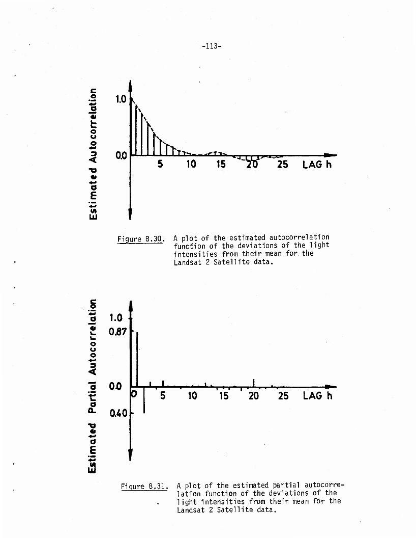
•113-
C o
1 •2 1.0 o % t_ o o o
o £ (A Id
0.0 I nth.,,„ rTV»
10 iTiDK LAGh
Figure 8.30. A plot of the estimated autocorrelation function of the deviations of the light intensities from their mean for:the Landsat 2 Satellite data.
a
o u o
<
r a a. "O
o E
10 4 0.87
0X>
0.40
J-U- 10
1-^ 1 i » i •
15 20 25 LAG h
Figure 8.31, A plot of the estimated partial autocorre- lation function of the deviations of the light intensities from their mean for the Landsat 2 Satellite data.
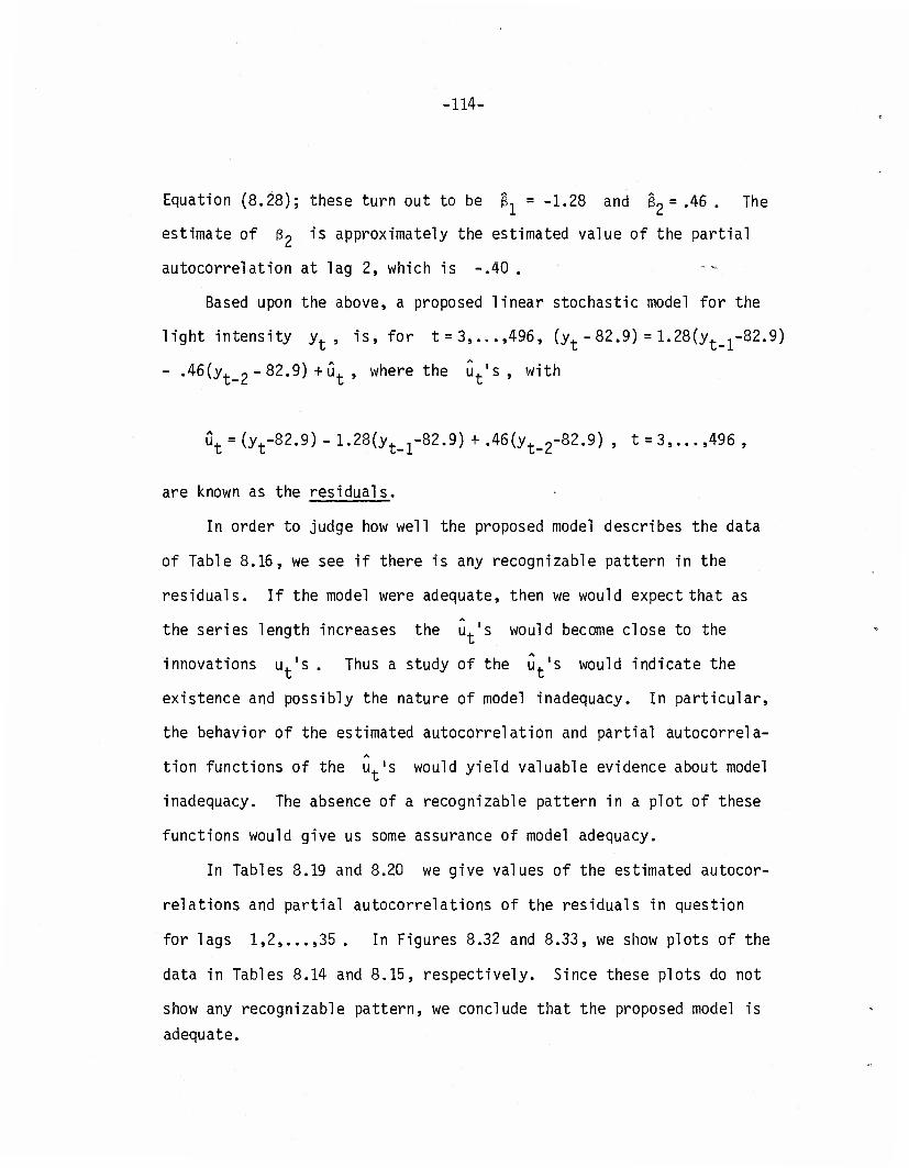
•114-
Equation (8.28); these turn out to be ^ = -1.28 and §2= .46 . The
estimate of Bo is approximately the estimated value of the partial
autocorrelation at lag 2, which is -.40 .
Based upon the above, a proposed linear stochastic model for the
light intensity yt , is, for t = 3 496, (yt - 82.9) = 1.28^^-82.9)
- •46(y._2 - 82.9) +u. , where the ut's , with
ut = (yt-82.9) - 1.28(yt_1-82.9) + .46(yt_2-82.9) , t = 3 496 ,
are known as the residuals.
In order to judge how well the proposed model describes the data
of Table 8.16, we see if there is any recognizable pattern in the
residuals. If the model were adequate, then we would expect that as
the series length increases the u.'s would become close to the
innovations u.'s . Thus a study of the ut's would indicate the
existence and possibly the nature of model inadequacy. In particular,
the behavior of the estimated autocorrelation and partial autocorrela-
tion functions of the u.'s would yield valuable evidence about model
inadequacy. The absence of a recognizable pattern in a plot of these
functions would give us some assurance of model adequacy.
In Tables 8.19 and 8.20 we give values of the estimated autocor-
relations and partial autocorrelations of the residuals in question
for lags 1,2,...,35 . In Figures 8.32 and 8.33, we show plots of the
data in Tables 8.14 and 8.15, respectively. Since these plots do not
show any recognizable pattern, we conclude that the proposed model is
adequate.

•115-
CM o CM
O O
CM O CO
CM
CO o ID
CO
-c cu —--o i. o
E £ o*~* •I- CM +Jv_^ CJ a: s="=t 3 rö
«4- +J c <o
C WO o •r E d) 4-> O -l-> r0 S- •!-
f— <*- T-
cr> CU r— «—i S- to CU • S_i— +•> OD O (0 18
U 3 00 CU O X5
I—— 4-> T- CM J3 3 to <B rO CU 4->
t— S- re T3 tO CU CÜ -o +•> x: s= «3 +-> rö E —I
•i- q_ POO) to x: <U +J «* Cum s- rno +j «M-
q- • o •
n CO CM CD * 3 .—1
« " >x:
CO
lO
«3- o
o o
CM o
o
CM o
o o
•vt- o
<3- o
in o
oo o
CM CM
CM
O CM
CM O
00
O
CM O
O
ID CM O
o
CM o
<3- o
co
oo CO
CM CO
O CO
CM
CO CM
I»» CM
CM
CM
O O
CM O
in o
CM o
CO o
o I
o
CO o
CM o
en re
to tu 3
05 rO
to CU 3
03 C7> r0
<4- O
to CU 3

-116-
< t=
CU c -a o O •i- £ +J o £= *—. 3 CM 4-
cc C <£ (O O 4-> •r- r0 +-> C T3 <Ö r0
r— CU CU £ +J 5- o •>- S- t-r- o q- i— o cu
o O (/j +J CM •P .— (0
3 re OO 00 <8 3
-a CM cu l~~ •!—
r— (O 10 4-> Xi •i- CU f0 (G -P i. oo h- S- "O
fd cu c o-x: ro
+J _i •a CU q_ <u -Pox: rO +J E
•i- « s- P Lf> O CO oo q- O) «
a> I XT . 4-> «
CM <4- .> O H
oo » a> x: 3
CM
-.0
5
:
'
CM
CM O •
1
i—1 I—1
CM O
1
OO CM
CM o LO
OO
I—I O
o T—1 o CM
CM
<—1 o
• 1
oo t—I o
en o o o
i—1 CM
o o OO oo
CM o
00 CM O •
O CM
o • 1
CM 00
un o •
r» o CD i—1
CM O i—1
00
OO 3 •
1
CO CM o »
00 1—1
o o OO O
IT) o • i—i
I—I o CT>
CM
O O
<* o « 1
CO OO o .
1
CO CM
o 1
CO ^3- O
Ln I—1 o CM
en o
CM <X> O
1 i—1
CM o <X)
CM
00 o
i
I—1 OO o 00
r-l OO o CM
OO o
Lag
h
S-
4- O
to CU 3
r— (0 >
x: en ro _l
x: s_ 4- O
t/1 CU 3
r— ro >
x; Di ro
—I
x: s- 4- O
CO cu 3
'rO >
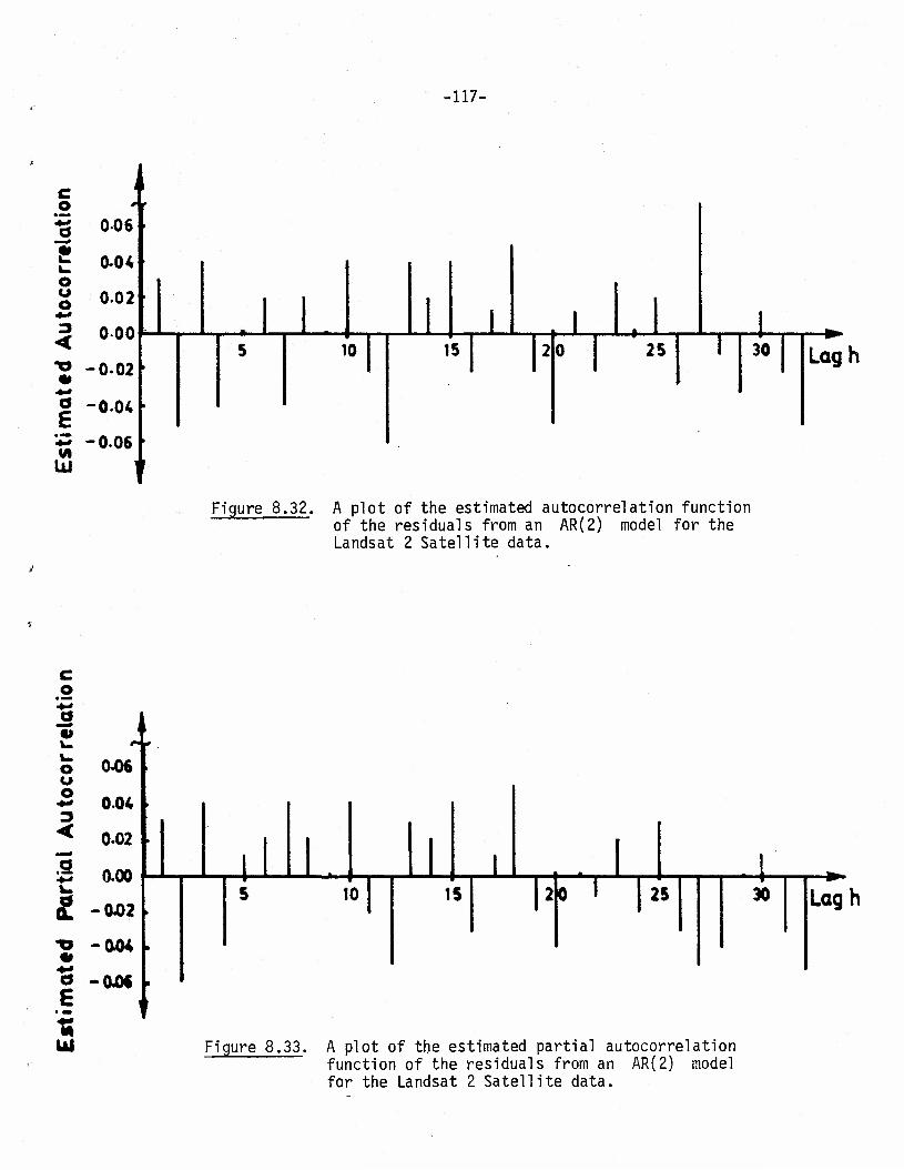
-117-
c o *
* 006
0-04 o o 0.02
4-*
3 <
000
*o -0-02 • «•*
o -0.04 E -0.06
M UJ i
i
10 15 25 30 Lagh
Figure 8.32. A plot of the estimated autocorrelation function of the residuals from an AR(2) model for the Landsat 2 Satellite data.
0 «1 v. *
O 04)6 o o +* 004 3 < 0.02 rl +* 0.00 V.
£ -O02
•o -004 • +* o -O0C E % ui
f
10 15 20 25 30 Lagh
Figure 8.33. A plot of the estimated partial autocorrelation function of the residuals from an AR(2) model for the Landsat 2 Satellite data.

-118-
References
Anderson, T. W. (1971). The Statistical Analysis of Time Series. New York: John Wiley & Sons, Inc.
Anderson, T. W. (1984). An Introduction to Multivariate Statistical Analysis, Second Edition. New York: John Wiley & Sons, Inc.
Box, G.E.P., and Jenkins, G.M. (1976). Time Series Analysis: fore- casting and control. San Francisco: Hoi den-Day.
Walker, G. (1931). On periodicity in series of related terms, Proc. Roy. Soc. London Ser. A, 131, 518-532.
Yule, G. U. (1927). On a method for investigating periodicities in disturbed series with special reference to Wolfer1s sunspot numbers, Phi los. Trans. Roy. Soc. London Ser. A, 226, 237-298.

UNCLASSIFIED SECURITY CLASSIFICATION OF THIS PAGE (When Date Entered)
REPORT DOCUMENTATION PAGE READ INSTRUCTIONS BEFORE COMPLETING FORM
I. REPORT NUMBER
12 2. GOVT ACCESSION NO. 3. RECIPIENT'S CATALOG NUMBER
4. TITLE fand Subtitle) S. TYPE OF REPORT & PERIOD COVERED
Methods and Applications of Time Series Analysis Part II: Linear Stochastic Models
Technical Report
6. PERFORMING ORG. REPORT NUMBER
7. AUTHORfaJ
T. W, Anderson and N. D. Singpurwalla
8. CONTRACT OR GRANT NUMBERfsJ
DAAG 29-82-K-0156
9. PERFORMING ORGANIZATION NAME AND ADDRESS
Department of Statistics - Sequoia Hall Stanford University Stanford, CA 94305
10. PROGRAM ELEMENT. PROJECT, TASK AREA 4 WORK UNIT NUMBERS
P-19065-M
11. CONTROLLING OFFICE NAME AND ADDRESS
U.S. Army Research Office Post Office Box 12211 Research Triangle Park, IC 27709
12. REPORT DATE October 1984
13. NUMBER OF PAGES 120 .
14. MONITORING AGENCY NAME ft ADDRESSf/f different from Controlling Office) IS. SECURITY CLASS, (of thta report)
UNCLASSIFIED
15a. DECLASSIFICATI ON/DOWNGRADING SCHEDULE
16. DISTRIBUTION STATEMENT (of this Report)
Approved for public release; distribution unlimited.
17. DISTRIBUTION STATEMENT (of the abstract entered In Block 20, It different from Report)
18. SUPPLEMENTARY NOTES
The view, opinions, and/or findings contained in this report are those of the authors and should not be construed as an official Department of the Army position, policy, or decision, unless so designated by other documentation.
19: KEY WORDS (Continue on reverse side it necessary and Identify by block number)
Time series analysis, autoregressive processes, moving average representation, autocorrelation function, partial autocorrelation function, forecasting
2Q. ABSTRACT (CootBoue en reverse aide It IKCMSOT rnxd. identity by block number)
This is the second in a series of technical reports developing the most modern procedures of time series analysis and forecasting for use in engineering, the physical sciences, and the social sciences. The exposition of methodology is based on a succinct presentation of the theoretical background and is illustrated with appropriate examples from engineering, maintenance and reliability, economics, and other physical and social sciences. This report is concerned with linear statistical models, especially autoregressive processes.
DD ^ST» 1473 EDITION OF 1 MOV 65 IS OBSOLETE UNCLASSIFIED SECURITY CLASSIFlCATrON OF THIS PAGE (When Data Entered)