.

DEVELOPMENT OF AN OPTICAL SYSTEM CALIBRATION AND ALIGNMENT METHODOLOGY USING SHACK-HARTMANN WAVEFRONT SENSOR

A THESIS SUBMITTED TO THE GRADUATE SCHOOL OF NATURAL AND APPLIED SCIENCES

OF THE MIDDLE EAST TECHNICAL UNIVERSITY

BY

FATİME ZEHRA ADİL

IN PARTIAL FULFILLMENT OF THE REQUIREMENTS FOR

THE DEGREE OF MASTER OF SCIENCE IN

MECHANICAL ENGINEERING

FEBRUARY 2013

.

Approval of the thesis:

DEVELOPMENT OF AN OPTICAL SYSTEM CALIBRATION AND ALIGNMENT METHODOLOGY USING SHACK-HARTMANN WAVEFRONT SENSOR

submitted by FATİME ZEHRA ADİL in partial fulfillment of the requirements for the degree of Master of Science in Mechanical Engineering Department, Middle East TechnicalUniversity by, Prof. Dr. Canan Özgen _____________________ Dean, Graduate School of Natural and Applied Sciences Prof. Dr. Süha Oral _____________________ Head of Department, Mechanical Engineering Assoc. Prof. Dr. İlhan Konukseven _____________________ Supervisor, Mechanical Engineering Dept., METU Prof. Dr. Tuna Balkan _____________________ Co-Supervisor, Mechanical Engineering Dept., METU Examining Committee Members: Prof. Dr. M. A. Sahir Arıkan _____________________ Mechanical Engineering Dept., METU Assoc. Prof. Dr. İlhan Konukseven _____________________ Mechanical Engineering Dept., METU Prof. Dr. Tuna Balkan _____________________ Mechanical Engineering Dept., METU Asst. Prof. Dr. A. Buğra Koku _____________________ Mechanical Engineering Dept., METU Devrim Anıl, Ph.D. _____________________ Mechanical and Optical Design Dept., ASELSAN

Date: 01.02.2013

iv

I hereby declare that all information in this document has been obtained and presented in accordance with academic rules and ethical conduct. I also declare that, as required by these rules and conduct, I have fully cited and referenced all material and results that are not original to this work.

Name, Last Name : Fatime Zehra Adil Signature :

v

.

ABSTRACT

DEVELOPMENT OF AN OPTICAL SYSTEM CALIBRATION AND ALIGNMENT METHODOLOGY USING SHACK-HARTMANN WAVEFRONT SENSOR

Adil, Fatime Zehra M.Sc. Department of Mechanical Engineering Supervisor: Assoc. Prof. Dr. İlhan Konukseven

Co-Supervisor: Prof. Dr. Tuna Balkan

February 2013, 80 pages

Shack-Hartmann wavefront sensors are commonly used in optical alignment, ophthalmology, astronomy, adaptive optics and commercial optical testing. Wavefront error measurement yields Zernike polynomials which provide useful data for alignment correction calculations.

In this thesis a practical alignment method of a helmet visor is proposed based on the wavefront error measurements. The optical system is modeled in Zemax software in order to collect the Zernike polynomial data necessary to relate the error measurements to the positioning of the visor. An artificial neural network based computer program is designed and trained with the data obtained from Zernike simulation in Zemax software and then the program is able to find how to invert the misalignments in the system. The performance of this alignment correction method is compared with the optical test setup measurements.

Keywords: Wavefront, Shack- Hartmann Sensor, Optical System Alignment, Zernike Polynomials

vi

.

ÖZ

SHACK-HARTMANN DALGACEPHESİ SENSÖRÜ KULLANILARAK OPTİK BİR SİSTEMİN KALİBRASYON VE HİZALAMASININ GELİŞTİRİLMESİ

Adil, Fatime Zehra Yüksek Lisans, Makina Mühendisliği Bölümü

Tez Yöneticisi: Doç. Dr. İlhan Konukseven Ortak Tez Yöneticisi: Prof. Dr. Tuna Balkan

Şubat 2013, 80 sayfa

Shack-Hartmann dalgacephesi sensorü, optik hizalama,optamoloji, astronomi, uyarlanabilir optik ve optik testler gibi alanlarda yaygın olarak kullanılmaktadır. Dalgacephesi hata ölçümü metodu ile hizalama hatalarınıdüzeltmek için kullanılan Zernike polinomları elde edilir.

Bu tezde, dalgacephesi hata ölçümü yoluyla kask vizörünün hizalanması için uygulamalı bir metot geliştirilmiştir. Zemax yazılımı kullanılarak optik sistem modellenmiştir vehata ölçümlerini vizörün konumu ile ilişkilendirmek için gerekli Zernike polinom verileri toplanmıştır. Yapay sinir ağı tabanlı bir bilgisayar programı tasarlanarak Zemax programından alınan Zernike verilerileri ile eğitilmiştir. Bu sayede yazılım ile hizalama hatalarını düzeltmek için gerekli adımlar hesaplanmıştır. Hata düzeltme algoritmasının performansı hazırlanan optik düzenek üzerinden alınan ölçümlerle karşılaştırılmıştır.

Anahtar Kelimeler: Dalgacephesi, Shack-Hartmann Sensörü, Optik Düzenek Hizalaması, Zernike Polinomları

vii

To my husband…

viii

.

ACKNOWLEDGEMENTS

I would like to express my sincere gratitude to my supervisor Assoc. Prof. Dr. İlhan Konukseven and my Co-supervisor Prof. Dr. Tuna Balkan for their guidance, patience and support. I am grateful to Aselsan Inc. for the support in this thesis study. I would like to thank Dr. Devrim Anıl for his continuous help, support and encouragement.

I would like to thank Esra Benli Öztürk and Burcu Barutçu for their valued friendship and support.

I can never thank enough my dear husband Ömer Faruk Adil for his infinite support, unending patience and unconditional eternal love.

I am deeply grateful to my family for making me who I am. I have felt their support behind me in each and every moment of my life.

ix

.

TABLE OF CONTENTS

ABSTRACT ............................................................................................................................................ v

ÖZ ..........................................................................................................................................................vi

ACKNOWLEDGEMENTS ................................................................................................................ viii

TABLE OF CONTENTS .......................................................................................................................ix

LIST OF TABLES ............................................................................................................................... xii

LIST OF FIGURES .............................................................................................................................. xii

LIST OF SYMBOLS ........................................................................................................................... xiv

LIST OF ABBREVIATIONS ............................................................................................................... xv

CHAPTERS

1 INTRODUCTION .................................................................................................................... 1

1.1 Problem Definition and Motivation ............................................................................ 1

1.2 State of The Art ........................................................................................................... 2

1.3 Structure of the Study ................................................................................................. 3

2 OPTICAL ABERRATION THEORY ...................................................................................... 5

2.1 Ray and Wavefront ..................................................................................................... 5

2.2 Law of Reflection ........................................................................................................ 5

2.3 Law of Refraction (Snell’s Law) ................................................................................. 6

2.4 Paraxial Optics (First Order Optics) ............................................................................ 7

2.5 Third Order Optics and Aberrations ............................................................................ 8

2.5.1 Defocus ..................................................................................................................... 10

2.5.2 Spherical Aberration ................................................................................................. 11

2.5.3 Coma ......................................................................................................................... 12

2.5.4 Astigmatism .............................................................................................................. 14

2.5.5 Field Curvature ......................................................................................................... 15

2.5.6 Distortion .................................................................................................................. 16

2.5.7 Chromatic Aberrations .............................................................................................. 17

3 OPTICAL METROLOGY TECHNOLOGIES ....................................................................... 19

3.1 Interferometry ........................................................................................................... 19

3.2 Focault Knife Edge Test............................................................................................ 21

3.3 Curvature Sensing ..................................................................................................... 22

3.4 Shack Hartmann Method........................................................................................... 22

3.4.1 Functional Principle .................................................................................................. 25

3.4.2 Advantages and Application Areas ........................................................................... 26

4 OPTICAL TEST SETUP DESIGN ......................................................................................... 29

4.1 Optical Path Alignment ............................................................................................. 31

x

4.2 Lens Centering .......................................................................................................... 32

4.3 5-DOF Holder for Visor ............................................................................................ 37

5 ALIGNMENT METHOD ....................................................................................................... 39

5.1 Zemax Model of the Optical Test Setup Design ....................................................... 39

5.1.1 Zemax Software ............................................................................................. 40

5.1.2 Integration of Internal Calibration into the Zemax Model ............................. 40

5.1.3 Training Data Generation in Zemax Software Simulation ............................ 42

5.2 Alignment Correction Method .................................................................................. 43

5.2.1 Artificial Neural Network (Feed Forward-Back Propagation) Method ......... 44

5.2.2 Training of the Neural Network..................................................................... 45

5.2.3 Calculation of Misalignments Using the Trained Network ........................... 47

5.2.4 An Implementation of the Alignment Method to the Real Test Setup ........... 48

6 CONCLUSION ....................................................................................................................... 53

REFERENCES ..................................................................................................................................... 55

APPENDICIES

A MATLAB CODE FOR ALIGNMENT CORRECTION SOFWARE ............................ 59

B ZEMAX MACRO CODE FOR TRAINING DATA GENERATION ............................ 75

C SHACK HARTMANN WAVEFRONT SENSOR ......................................................... 77

D CALIBRATION AND TEST PROCEDURE OF THE VISOR ALIGNMENT TEST SETUP ................................................................................................................................... 79

xi

..

LIST OF TABLES

TABLES

Table 1 List of Zernike Coefficients .................................................................................................... 10

Table 2 Optical Test Setup System İnternal Error ............................................................................... 42

Table 3 An Example of First Wavefront Measurement to Fall on the SHWS ..................................... 48

Table 4 An Example of Corrected Wavefront Measurement .............................................................. 49

Table A. 1 Training Part of the MATLAB Code ................................................................................ 59

Table A. 2 Misalignment Calculation Interface Part of the MATLAB Code .................................... 61

Table B. 1 Zemax ZPL Macro Code .................................................................................................. 75

Table C. 1 Shack Hartmann Wavefront Sensor Camera Specifications .............................................. 77

Table C. 2 Shack Hartmann Wavefront Sensor General Specifications .............................................. 78

Table D. 1Equipment List ................................................................................................................... 79

xii

.

LIST OF FIGURES

FIGURES

Figure 1 The model of helmet module and the visor ............................................................................. 1

Figure 2 Differences of rays and wavefront .......................................................................................... 6

Figure 3 Illustration of reflection and refraction ................................................................................... 6

Figure 4 Formation of a perfect image .................................................................................................. 7

Figure 5 Image formation in third oreder optics ................................................................................... 8

Figure 6 Illustration of ray and wave aberrations .................................................................................. 9

Figure 7 Unit circle for Zernike polynomials ......................................................................................... 9

Figure 8 A defocused and focused images .......................................................................................... 11

Figure 9 Formation of spherical aberation ........................................................................................... 11

Figure 10 Paraxial rays are focused in the region nearer to the lens ................................................... 12

Figure 11 Image formed by a system having coma aberration ............................................................ 13

Figure 12 Rays through the outer portions of the lens focus at a different height than the

rays through the center of the lens ....................................................................................................... 13

Figure 13 Illustration of an astigmatism case ...................................................................................... 14

Figure 14 Primary astigmatism of a simple lens ................................................................................. 15

Figure 15 Illustration of field curvature .............................................................................................. 15

Figure 16 Positive distortion formation ............................................................................................... 16

Figure 17 Pincushion and barrel distortion of a rectilinear object ....................................................... 16

Figure 18 Lateral and axial chromatic aberration ................................................................................ 17

Figure 19 An illustration of the Newtonian Fringes ............................................................................ 20

Figure 20 Schematics of an interferometer ......................................................................................... 20

Figure 21 Schematic of the Focault Knife Edge Test .......................................................................... 21

Figure 22 Hartmann test perspective schematics showing the Hartmann screen over a

mirror to be tested ................................................................................................................................ 23

Figure 23 Hartmann test schematics of a concave mirror test .............................................................. 23

Figure 24Array of microlens screen ..................................................................................................... 24

Figure 25 Relation between the transverse aberrations and the wavefront deformations ................... 24

Figure 26 Operation of the wavefront sensor ...................................................................................... 25

Figure 27 Detailed operation of the Shack Hartmann sensor .............................................................. 26

Figure 28 Sketch of the optical test setup ............................................................................................. 29

Figure 29 Final configuration of the optical test setup ......................................................................... 30

Figure 30 Pinhole diaphragms used for alignment of the optical test setup ......................................... 31

xiii

Figure 31 Optical test setup alignment accuracy calculation .............................................................. 31

Figure 32 Optical test setup alignment configuration.......................................................................... 32

Figure 33 Zemax 3D layout of the objective part ................................................................................ 32

Figure 34 Zemax lens data editor of the objective design ................................................................... 33

Figure 35 Cut view of the objective includes optical and mechanical parts ........................................ 33

Figure 36 Optical centering machine ................................................................................................. 34

Figure 37 Centering measurement result of the initially manufactured objective ............................... 35

Figure 38 Centering measurement of the remanufactured right objective .......................................... 36

Figure 39 Centering measurement of the remanufactured left objective ............................................. 36

Figure 40 Visor parts and visor frame ................................................................................................. 37

Figure 41 Visor with reflecting coating ............................................................................................... 37

Figure 42 5 DOF Visor Holder ............................................................................................................ 38

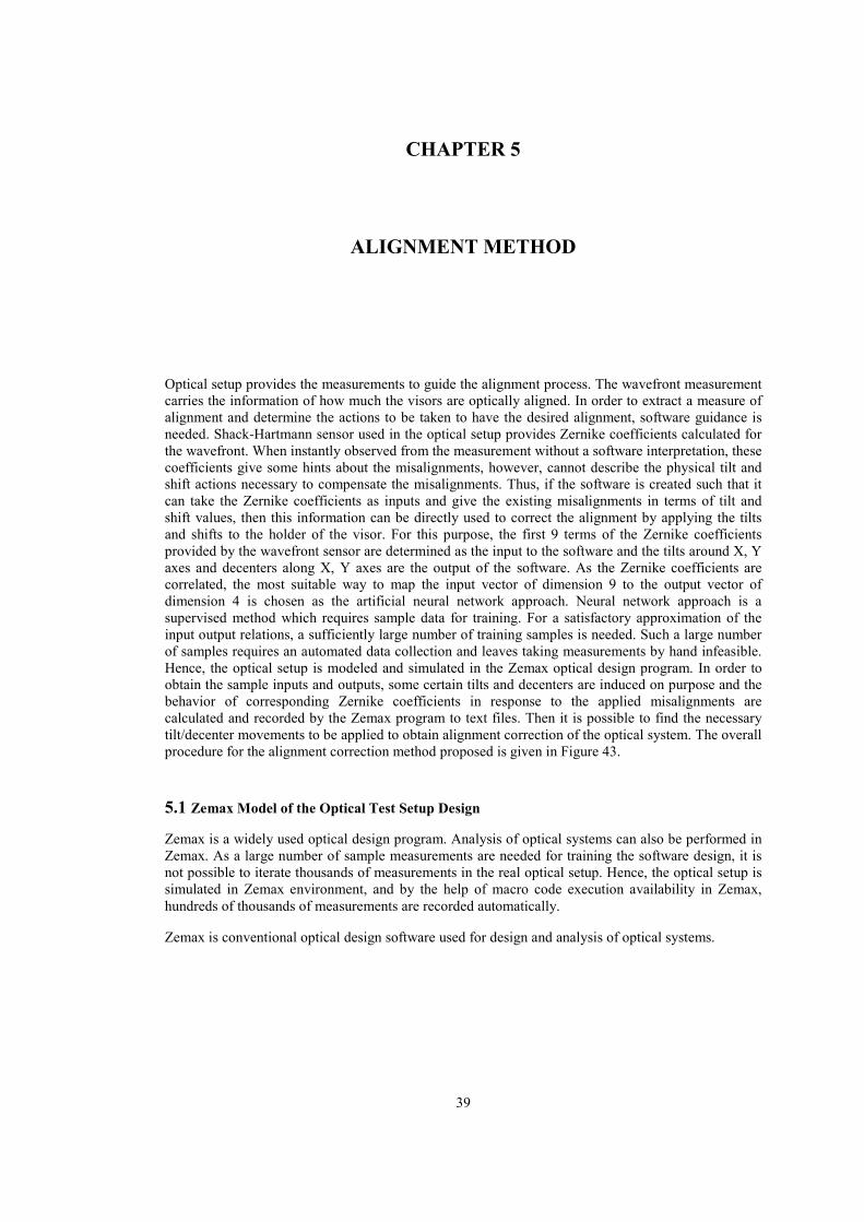
Figure 43 Alignment correction procedure ......................................................................................... 40

Figure 44Setup internal calibration ..................................................................................................... 41

Figure 45Pinholes for objective alignment .......................................................................................... 41

Figure 46Alignment correction method summary ............................................................................... 43

Figure 47Artificial neural network examples. (a) Feed forward structure, (b) Recurrent structure ... 44

Figure 48Feed forward neural network structure ............................................................................... 45

Figure 49Back propagation of output errors ....................................................................................... 46

Figure 50Training of the network in MATLAB .................................................................................. 46

Figure 51Error performance of the network training .......................................................................... 47

Figure 52Graphical interface for alignment correction software ......................................................... 48

Figure 53 An example of first appearance of laser beam on the SHWS ............................................. 49

Figure 54 An example of misalignment calculation ............................................................................ 50

Figure 55 An example of wavefront shape of the misaligned visor .................................................... 50

Figure 56 An example of wavefront shape of the aligned visor .......................................................... 51

Figure C. 1 Thorlabs WFS150-5C Shack Hartman Wavefront Sensor ............................................... 77

xiv

.

LIST OF SYMBOLS

�� Angle of incidence

�� Angle of reflectance

�� Angle of transmittance

�� Refractive index of incident medium

�� Refractive index of transmitted medium

��′� Transverse spherical aberration

�′� Longitudinal spherical aberration

Shape factor

� Image height

�� Paraxial image height

(�, �) Wavefront shape function

��� Focal length of a micro lens

xv

.

LIST OF ABBREVIATIONS

HICS Helmet Integrated Cueing System

OAP Off Axis Parabolic

IIT Image Intensifier Tube

OPD Optical Path Difference

SHWS Shack Hartmann Wavefront Sensor

xvi

1

.

CHAPTER 1

INTRODUCTION

1.1 Problem Definition and Motivation

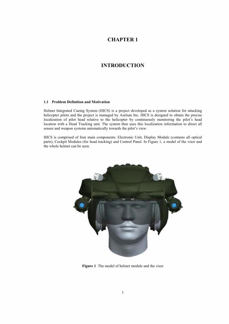
Helmet Integrated Cueing System (HICS) is a project developed as a system solution for attacking helicopter pilots and the project is managed by Aselsan Inc. HICS is designed to obtain the precise localization of pilot head relative to the helicopter by continuously monitoring the pilot’s head location with a Head Tracking unit. The system then uses this localization information to direct all sensor and weapon systems automatically towards the pilot’s view. HICS is comprised of four main components: Electronic Unit, Display Module (contains all optical parts), Cockpit Modules (for head tracking) and Control Panel. In Figure 1, a model of the visor and the whole helmet can be seen.

Figure 1 The model of helmet module and the visor

2

The helmet designed for the helicopter pilots as part of the project AVCI also features night vision capability. In order not to limit or block the sight of the pilot while providing night vision display, a transparent visor is used. An optical coating process is applied to the circular region around the central part of the visor for the purpose of gaining a reflectance of 40%. This makes it possible for the image from the night vision channel to finally reach to the observing eye right after the reflecting region located at the center of the visor. Due to its direct effect on the image reaching the observing eye of the pilot, the sensitivity to be ensured between the visors is of utmost importance. The night vision image is reflected from the coated part of the visor. This reflected image must coincide with the regular human sight image seen through the non-reflecting regions of the visor. To coincide the night vision with the sight image, the night vision image must also be seen in 3-D by the pilot as in the regular human sight image. For the purpose of 3-D sight, both of the eyes must be fed with images from separate channels. The helmet produced by Aselsan contains two separate image intensifier tubes and two separate optical channels. The image leaving the optical channel ends up being reflected from the visor as the last element before the eye and then the image reaches the observing eye. This makes the alignment of the visor part very critical. If the visor parts are not properly aligned, the night vision image and the sight image do not coincide. For this reason, the pilot’s brain needs overprocessing in order to coincide and interpret the two images. This overprocessing eventually causes heavy headaches and fuzzy sight for the pilot. The visor is composed of two sections; one for the left and one for the right eye and it is produced by the method of plastic injection. With this method, as the desired sensitivity of tilt, decenter and defocus parameters between the two visor cannot be satisfied, the visors have to be produced separately. The mentioned sensitivity of parameters required between the visors is very crucial due to its effect on the image seen by the pilot. Moreover, it can be seen that it is a common practice among other helmet providers from other countries to produce the visors in two separate segments and to align them using optical methods. For the alignment, the two segments of the visors are first positioned on a vacuum pad. Vacuum pad makes it possible to hold the segments which have spherical surfaces without damaging and slipping. The initial positioning of the visors on the vacuum pads differs randomly in each placement. For the measurement of the initial misalignment and changes during the alignment process, an optical wavefront analyzer, namely Shack-Hartmann is used. Based on the wavefront measurements, the misalignment is observed and to place the visors at desired positions precisely, some tilt and decenter changes are applied to the initial position of the visors by the help of 5-axis holders that the vacuum pads are attached to. But this process would require a lot of trials and errors if the sequence of adjustments necessary for the correction of alignment is not known. Hence, in this study, in addition to measurement of the misalignments with Shack-Hartmann wavefront sensor, a correction procedure is proposed which is the software that learns the measurements corresponding to certain incorrect positioning. After the software is trained, it gets the measurement and returns the necessary corrections at once. The software is a Neural Network based program which needs training. For the training, a comprehensive set of measurement data collection is required. It is not practical to collect sufficient and well-ranged positioning data from the actual optical setup. Thus, a computer simulation of the optical system is modeled by the use of Zemax software which is a well-known optical design tool. A Zemax model of the optical system provided sufficient data relating the tilt and decenter misalignments to the wavefront measurements. After that data is fed to the Neural Network training, the correction software is built and it gets the wavefront measurements and returns the necessary tilt and decenter adjustments to align the visors.

1.2 State of the Art

There is a wide variety of applications on optical alignment methods which use wavefront analysis. In their work, Neal and Mansel [1] proposed an alignment method for a 24-inch telescope. The alignment process is performed by hand in an iterative manner. Ruda, presented a wavefront based alignment an off axis aspheric surfaces [2]. A common usage of Shack-Hartmann sensor is encountered in measurement of the aberrations of human eye. Liang et al. [3] worked on measurement of wave aberrations of the human eye. In this study, aberrations of the eye are modeled by making use

3

of the measured Zernike coefficients. Another related application can be seen on optical metrology. Forest et al. [4] has developed a Shack-Hartmann surface metrology method to measure surface flatness of optic foils. An automatic OAP mirror alignment and deformable mirror alignment method was proposed by Orlenko et al. [5] and Baumhaker et al. [6] respectively. The technique is based on measuring the wavefront by the Shack–Hartmann method and correcting the wavefront by applying voltage to the distorted wavefront part of the bimorph mirror. Therefore they used the bimorph material property to refine the wavefront. Lundgren et al. [7] suggested a method for alignment of three off axis parabolic telescope mirrors. In this early method, instead of Shack-Hartmann wavefront sensor a 5-hole Hartmann screen and position sensing detector were used for measurement. A least squares optimization approach was used in the software that models the measurements and misalignments relation. A more recent study about software guidance for alignment is performed by Gao et al. [8] He suggests a method of alignment calculation of a reference transmission sphere of an interferometer. In this study, a collection of sensitive variables are chosen in relation to Zernike coefficients to interpret the optical errors. Then corrections are calculated based on an inverse operation. However, this method focuses only on the most sensitive parameters chosen by the author one by one; the combined effect of all the parameters is not included. When all the related works are considered, some of the older methods rely on successive iterations of corrections; other techniques which have computer aided correction are based on purely experimental data collection for their software. In this study, large number of data samples is required. This makes experimental data collection impractical. In fact, if so many experimental data could be obtained, then such a computer based method would not be needed. Thus training data is obtained by using Zemax software which enables generating many data samples. In this way, a robust construction of the relation between the Zernike measurements and alignment corrections such as tilt and decenter is obtained. As the software is designed as a learning program, it stands as an adaptive solution applicable to other problems by training the software with the relevant data.

1.3 Structure of the Study

Brief information about the helmet system the problem definition and alignment model is described in first part of the introduction. The state of art is mentioned in the second section of the introduction part. In chapter 2 the optical aberration theory, causes and results of the misalignment have been discussed. At first, the basics of aberration theory in optics are explained. Then the difference between paraxial optics and third order optics is presented. Finally kinds of aberrations have explained. In chapter 3 optical metrology technologies which are used for testing the optical surface quality have been explained, and the theory of Shack-Hartmann wavefront sensor and the wavefront interpretations are investigated and presented. In chapter 4 the experimental setup design, specifications and the basic parameters of the helmet visors which are used for the alignment procedure are given. In chapter 5 optical set up measurements, simulations representing the optical set up in Zemax software are represented. The software based alignment procedure is explained in detail, and the final wavefront measurements are given. Finally, the method has been overviewed; discussions and recommendations are made for the future works.

4

5

.

CHAPTER 2

OPTICAL ABERRATION THEORY

For an optical system the optimal case is when all the optical components in the system lie on an imaginary axis called optical axis. Formally optical axis is defined as an imaginary line passing through the geometrical center of the radially symmetrical optical components in the system. The arrangement of the optical components on such an optical axis is called optical alignment. The alignment of an optical system is of critical importance for the sensitivity of the system. Any deviations from the ideal alignment will result in misalignment. Misalignments are mainly caused by decenter, despace, tip-tilt or any combination of these deviations from optical axis. Hence it is necessary to minimize misalignments in the system in order to maintain precision. It is essential to mention optical aberrations when dealing with alignment. If the reasons and results of aberrations are known, corrections on alignment can be considered accordingly. Usually, misalignment reveals itself as image deformations such as blurred image on the focal plane or image not falling onto the focal plane at all. In the following section, optical aberrations are explained in more detail.

2.1 Ray and Wavefront

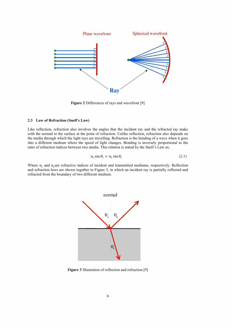
In optics, rays are ideal lines emerging from the source and represent the direction of propagation throughout the line. On the other hand wavefronts are formed from combination of the points which have same phase on the ray. Therefore wavefronts are imaginary surfaces which model the points having same phase of a wave. Certain properties of light determine the shape of wavefront surface. For instance, a circular wavefront have a point source or gain power after pass through a lens or a different optical element. On the other side a plane wavefront generally have an extended source or meet a collimator surface. In Figure 2 rays, wavefronts and the differences between them are shown. The most important relation between rays and wave fronts is rays are always perpendicular to the wavefronts.

2.2 Law of Reflection

The law of reflection states that when a ray is reflected from a boundary of two different medium, the reflected ray stays within the same medium. The ray of light that comes to a separation of the different medium is known as the incident ray. The ray of light that leaves the interface is named as the reflected ray. At the point of incidence where the ray makes a contact with the interface, a line can be drawn perpendicular to the separation of the medium. This line is known as a normal line. The normal line divides the angle between the incident ray and the reflected ray into two equal angles. In Figure 3

the angle of incidence θi is equal to the angle of reflection θr.

6

Figure 2 Differences of rays and wavefront [9]

2.3 Law of Refraction (Snell’s Law)

Like reflection, refraction also involves the angles that the incident ray and the refracted ray make with the normal to the surface at the point of refraction. Unlike reflection, refraction also depends on the media through which the light rays are travelling. Refraction is the bending of a wave when it goes into a different medium where the speed of light changes. Bending is inversely proportional to the ratio of refraction indices between two media. This relation is stated by the Snell’s Law as;

�� sin �� = � sin � (2.1)

Where �� and �are refractive indices of incident and transmitted mediums, respectively. Reflection and refraction laws are shown together in Figure 3, in which an incident ray is partially reflected and refracted from the boundary of two different medium.

Figure 3 Illustration of reflection and refraction [9]

7

2.4 Paraxial Optics (First order optics)

Paraxial optics, also known as the Gaussian optics, describes the propagation behavior of light along an optical system in the case of rays being near the optical axis. The most common way to introduce the paraxial approach is by approximations of the trigonometric functions. It is well known that sine,

cosine, and tangent functions can be expanded as power series around the angle of reflection, � = 0. These expansions are;

sin � = � −��

3!+

��

5!−

��

7!+

��

9!+ ⋯

(2.2)

cos � = 1 −��

2!+

��

4!−

��

6!+

�

8!− ⋯

(2.3)

tan � = � +��

3!+

��

5!+

��

7!+

��

9!+ ⋯

(2.4)

The paraxial values of the trigonometric functions are given by;

sin � ≅ � (2.5)

cos � ≅ 1 (2.6)

tan � ≅ � (2.7)

With the light of the paraxial optics, sine function is simplified to the angle itself and the Snell Law becomes;

���� = �� (2.8)

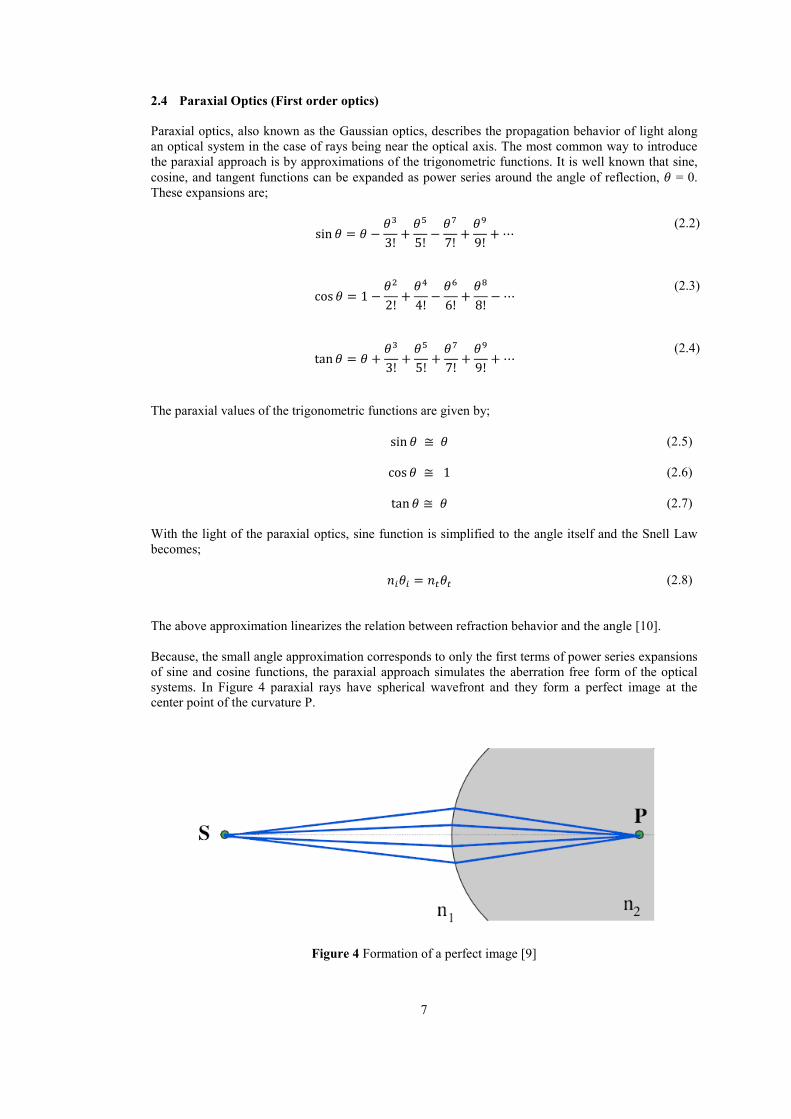
The above approximation linearizes the relation between refraction behavior and the angle [10]. Because, the small angle approximation corresponds to only the first terms of power series expansions of sine and cosine functions, the paraxial approach simulates the aberration free form of the optical systems. In Figure 4 paraxial rays have spherical wavefront and they form a perfect image at the center point of the curvature P.

Figure 4 Formation of a perfect image [9]

8

2.5 Third Order Optics and Aberrations

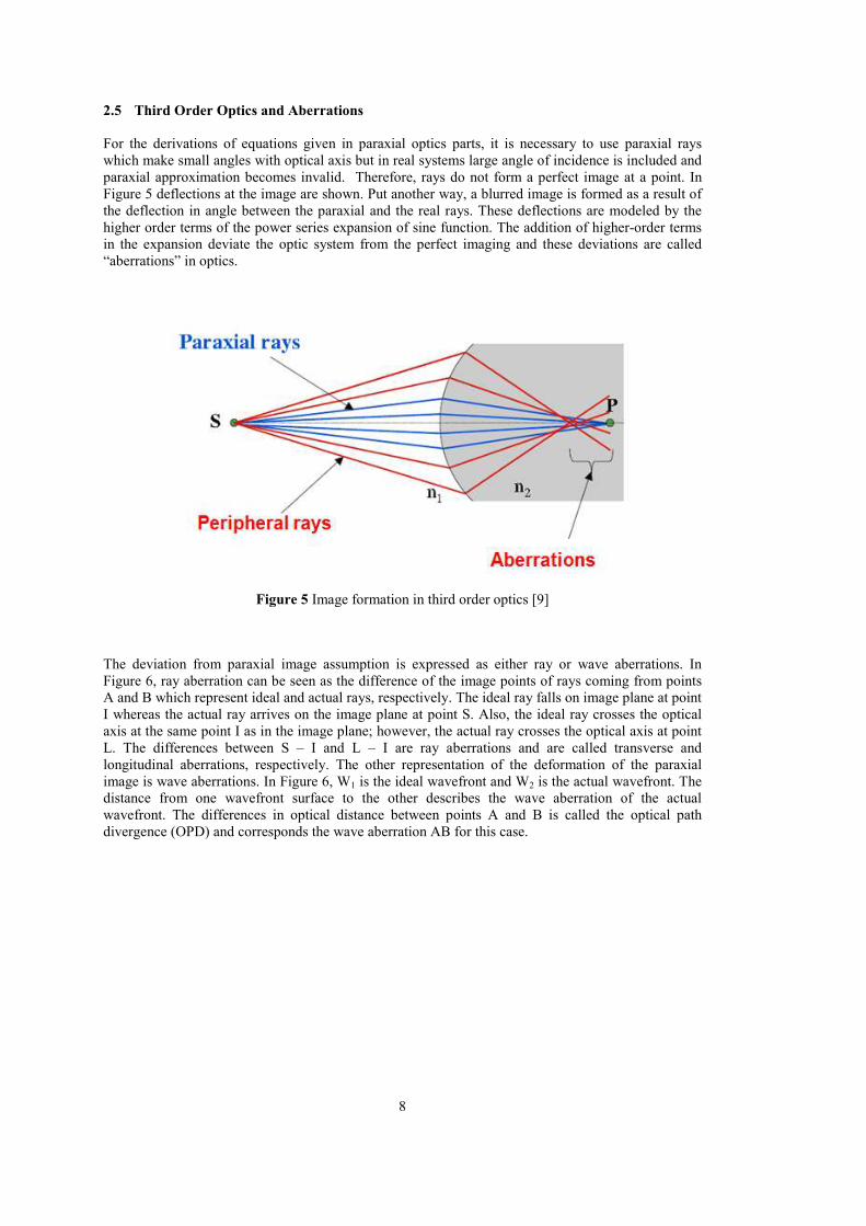
For the derivations of equations given in paraxial optics parts, it is necessary to use paraxial rays which make small angles with optical axis but in real systems large angle of incidence is included and paraxial approximation becomes invalid. Therefore, rays do not form a perfect image at a point. In Figure 5 deflections at the image are shown. Put another way, a blurred image is formed as a result of the deflection in angle between the paraxial and the real rays. These deflections are modeled by the higher order terms of the power series expansion of sine function. The addition of higher-order terms in the expansion deviate the optic system from the perfect imaging and these deviations are called “aberrations” in optics.

Figure 5 Image formation in third order optics [9]

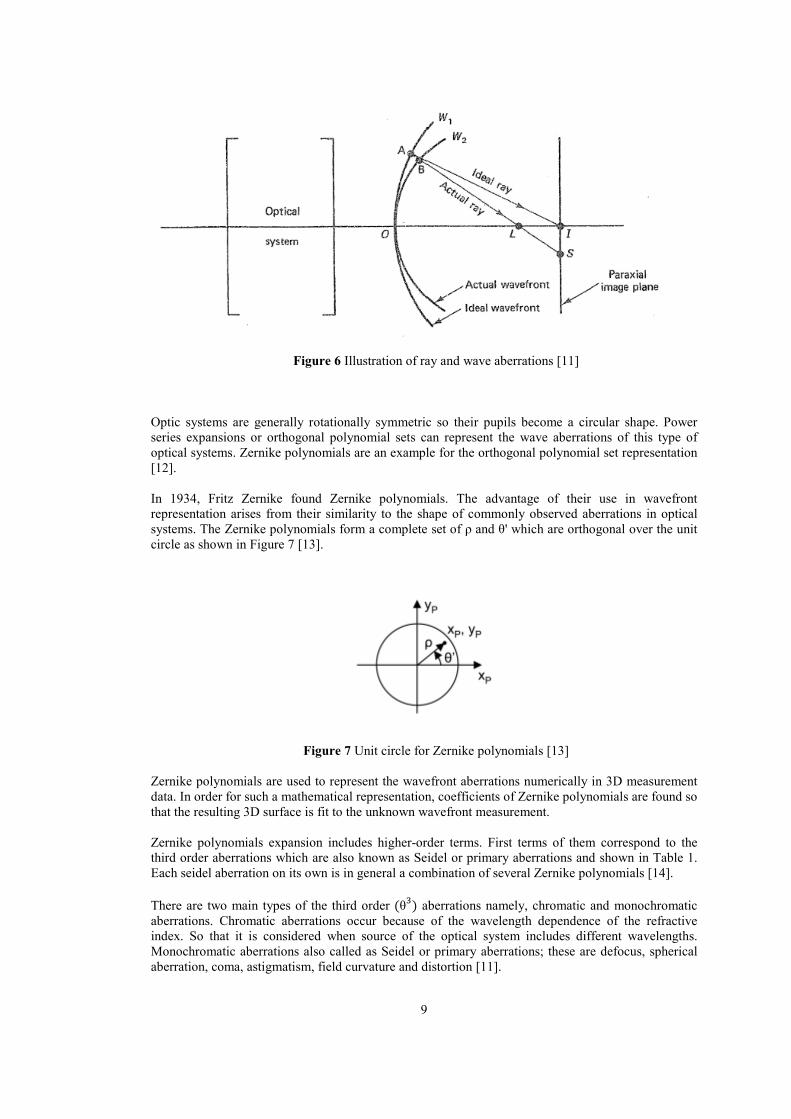
The deviation from paraxial image assumption is expressed as either ray or wave aberrations. In Figure 6, ray aberration can be seen as the difference of the image points of rays coming from points A and B which represent ideal and actual rays, respectively. The ideal ray falls on image plane at point I whereas the actual ray arrives on the image plane at point S. Also, the ideal ray crosses the optical axis at the same point I as in the image plane; however, the actual ray crosses the optical axis at point L. The differences between S – I and L – I are ray aberrations and are called transverse and longitudinal aberrations, respectively. The other representation of the deformation of the paraxial image is wave aberrations. In Figure 6, W1 is the ideal wavefront and W2 is the actual wavefront. The distance from one wavefront surface to the other describes the wave aberration of the actual wavefront. The differences in optical distance between points A and B is called the optical path divergence (OPD) and corresponds the wave aberration AB for this case.

9

Figure 6 Illustration of ray and wave aberrations [11] Optic systems are generally rotationally symmetric so their pupils become a circular shape. Power series expansions or orthogonal polynomial sets can represent the wave aberrations of this type of optical systems. Zernike polynomials are an example for the orthogonal polynomial set representation [12]. In 1934, Fritz Zernike found Zernike polynomials. The advantage of their use in wavefront representation arises from their similarity to the shape of commonly observed aberrations in optical systems. The Zernike polynomials form a complete set of ρ and θ' which are orthogonal over the unit circle as shown in Figure 7 [13].

Figure 7 Unit circle for Zernike polynomials [13] Zernike polynomials are used to represent the wavefront aberrations numerically in 3D measurement data. In order for such a mathematical representation, coefficients of Zernike polynomials are found so that the resulting 3D surface is fit to the unknown wavefront measurement. Zernike polynomials expansion includes higher-order terms. First terms of them correspond to the third order aberrations which are also known as Seidel or primary aberrations and shown in Table 1. Each seidel aberration on its own is in general a combination of several Zernike polynomials [14].

There are two main types of the third order (θ�

) aberrations namely, chromatic and monochromatic aberrations. Chromatic aberrations occur because of the wavelength dependence of the refractive index. So that it is considered when source of the optical system includes different wavelengths. Monochromatic aberrations also called as Seidel or primary aberrations; these are defocus, spherical aberration, coma, astigmatism, field curvature and distortion [11].

10

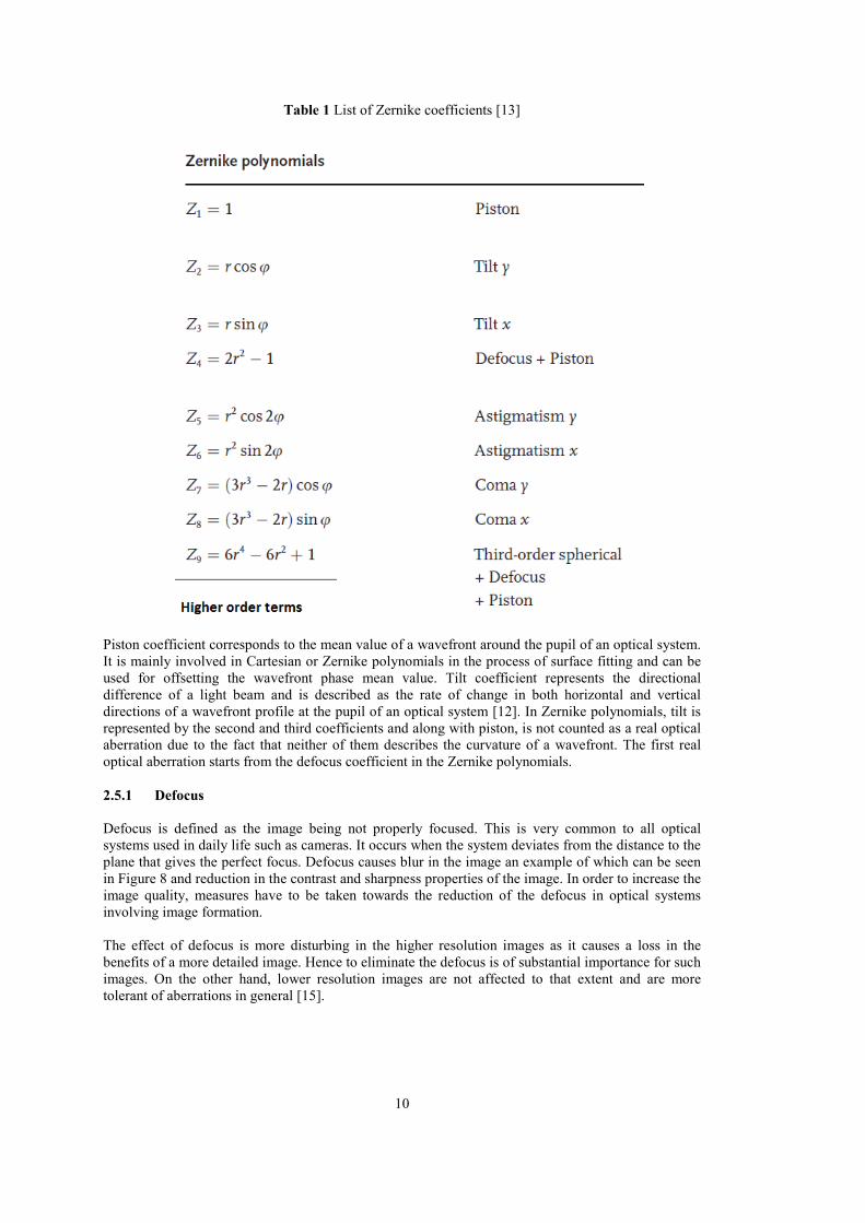
Table 1 List of Zernike coefficients [13]

Piston coefficient corresponds to the mean value of a wavefront around the pupil of an optical system. It is mainly involved in Cartesian or Zernike polynomials in the process of surface fitting and can be used for offsetting the wavefront phase mean value. Tilt coefficient represents the directional difference of a light beam and is described as the rate of change in both horizontal and vertical directions of a wavefront profile at the pupil of an optical system [12]. In Zernike polynomials, tilt is represented by the second and third coefficients and along with piston, is not counted as a real optical aberration due to the fact that neither of them describes the curvature of a wavefront. The first real optical aberration starts from the defocus coefficient in the Zernike polynomials.

2.5.1 Defocus

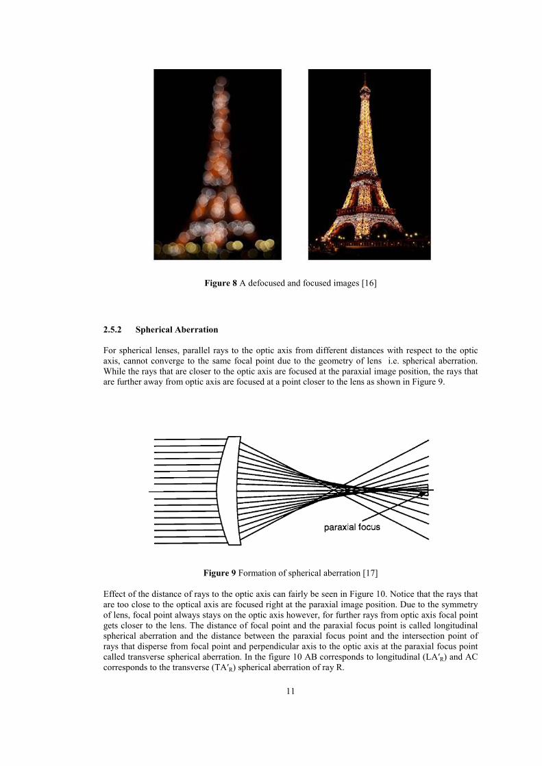
Defocus is defined as the image being not properly focused. This is very common to all optical systems used in daily life such as cameras. It occurs when the system deviates from the distance to the plane that gives the perfect focus. Defocus causes blur in the image an example of which can be seen in Figure 8 and reduction in the contrast and sharpness properties of the image. In order to increase the image quality, measures have to be taken towards the reduction of the defocus in optical systems involving image formation. The effect of defocus is more disturbing in the higher resolution images as it causes a loss in the benefits of a more detailed image. Hence to eliminate the defocus is of substantial importance for such images. On the other hand, lower resolution images are not affected to that extent and are more tolerant of aberrations in general [15].

11

Figure 8 A defocused and focused images [16]

2.5.2 Spherical Aberration

For spherical lenses, parallel rays to the optic axis from different distances with respect to the optic axis, cannot converge to the same focal point due to the geometry of lens i.e. spherical aberration. While the rays that are closer to the optic axis are focused at the paraxial image position, the rays that are further away from optic axis are focused at a point closer to the lens as shown in Figure 9.

Figure 9 Formation of spherical aberration [17]

Effect of the distance of rays to the optic axis can fairly be seen in Figure 10. Notice that the rays that are too close to the optical axis are focused right at the paraxial image position. Due to the symmetry of lens, focal point always stays on the optic axis however, for further rays from optic axis focal point gets closer to the lens. The distance of focal point and the paraxial focus point is called longitudinal spherical aberration and the distance between the paraxial focus point and the intersection point of rays that disperse from focal point and perpendicular axis to the optic axis at the paraxial focus point called transverse spherical aberration. In the figure 10 AB corresponds to longitudinal (LA′R) and AC corresponds to the transverse (TA′R) spherical aberration of ray R.

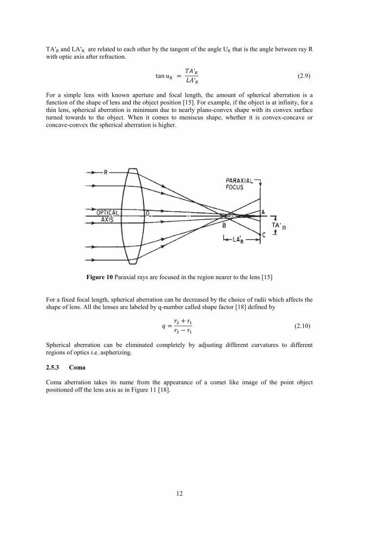
12

TA′R and LA′R are related to each other by the tangent of the angle UR that is the angle between ray R with optic axis after refraction.

tan '( = )*′(

+*′( (2.9)

For a simple lens with known aperture and focal length, the amount of spherical aberration is a function of the shape of lens and the object position [15]. For example, if the object is at infinity, for a thin lens, spherical aberration is minimum due to nearly plano-convex shape with its convex surface turned towards to the object. When it comes to meniscus shape, whether it is convex-concave or concave-convex the spherical aberration is higher.

Figure 10 Paraxial rays are focused in the region nearer to the lens [15]

For a fixed focal length, spherical aberration can be decreased by the choice of radii which affects the shape of lens. All the lenses are labeled by q-number called shape factor [18] defined by

, =-� + -.

-� − -.

(2.10)

Spherical aberration can be eliminated completely by adjusting different curvatures to different regions of optics i.e. aspherizing.

2.5.3 Coma

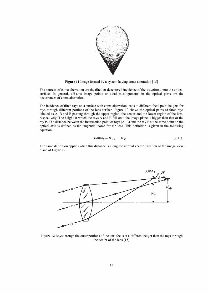
Coma aberration takes its name from the appearance of a comet like image of the point object positioned off the lens axis as in Figure 11 [18].

13

Figure 11 Image formed by a system having coma aberration [15]

The sources of coma aberration are the tilted or decentered incidence of the wavefront onto the optical surface. In general, off-axis image points or axial misalignments in the optical parts are the occurrences of coma aberration. The incidence of tilted rays on a surface with coma aberration leads to different focal point heights for rays through different portions of the lens surface. Figure 12 shows the optical paths of three rays labeled as A, B and P passing through the upper region, the center and the lower region of the lens, respectively. The height at which the rays A and B fall onto the image plane is bigger than that of the ray P. The distance between the intersection point of rays (A, B) and the ray P at the same point on the optical axis is defined as the tangential coma for the lens. This definition is given in the following equation:

/012 = 3′45 − 3′6 (2.11)

The same definition applies when this distance is along the normal vector direction of the image view plane of Figure 12.

Figure 12 Rays through the outer portions of the lens focus at a different height than the rays through

the center of the lens [15]

14

For on axially symmetric system, coma aberration is zero on the optic axis and can be eliminated by choosing appropriate shape of lens and suitable position of apertures that limits the image forming rays.

2.5.4 Astigmatism

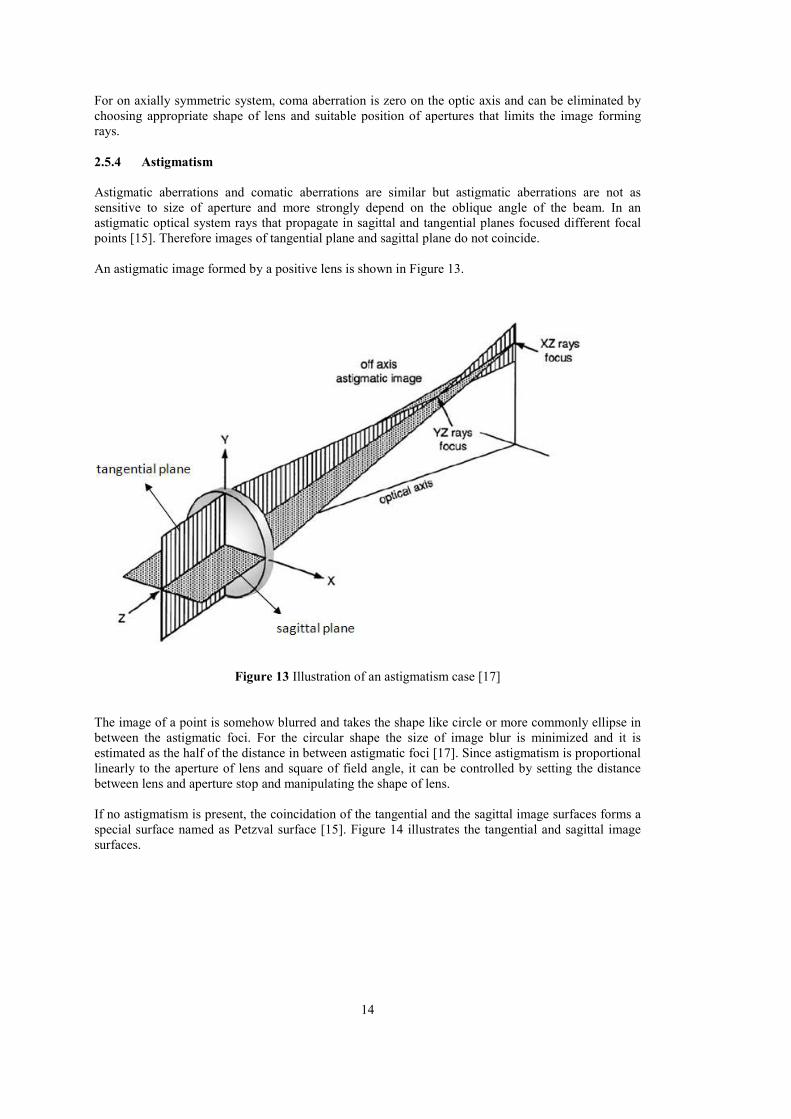
Astigmatic aberrations and comatic aberrations are similar but astigmatic aberrations are not as sensitive to size of aperture and more strongly depend on the oblique angle of the beam. In an astigmatic optical system rays that propagate in sagittal and tangential planes focused different focal points [15]. Therefore images of tangential plane and sagittal plane do not coincide.

An astigmatic image formed by a positive lens is shown in Figure 13.

Figure 13 Illustration of an astigmatism case [17]

The image of a point is somehow blurred and takes the shape like circle or more commonly ellipse in between the astigmatic foci. For the circular shape the size of image blur is minimized and it is estimated as the half of the distance in between astigmatic foci [17]. Since astigmatism is proportional linearly to the aperture of lens and square of field angle, it can be controlled by setting the distance between lens and aperture stop and manipulating the shape of lens. If no astigmatism is present, the coincidation of the tangential and the sagittal image surfaces forms a special surface named as Petzval surface [15]. Figure 14 illustrates the tangential and sagittal image surfaces.

15

Figure 14 Primary astigmatism of a simple lens [15] For this case, there is primary astigmatism in which tangential and sagittal planes do not coincide. However, astigmatism can be eliminated by appropriate choice of lens shapes and distances between lenses.

2.5.5 Field Curvature

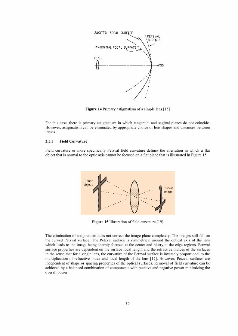
Field curvature or more specifically Petzval field curvature defines the aberration in which a flat object that is normal to the optic axis cannot be focused on a flat plane that is illustrated in Figure 15

Figure 15 Illustration of field curvature [19]

The elimination of astigmatism does not correct the image plane completely. The images still fall on the curved Petzval surface. The Petzval surface is symmetrical around the optical axis of the lens which leads to the image being sharply focused at the center and blurry at the edge regions. Petzval surface properties are dependent on the surface focal length and the refractive indices of the surfaces in the sense that for a single lens, the curvature of the Petzval surface is inversely proportional to the multiplication of refractive index and focal length of the lens [17]. However, Petzval surfaces are independent of shape or spacing properties of the optical surfaces. Removal of field curvature can be achieved by a balanced combination of components with positive and negative power minimizing the overall power.

16

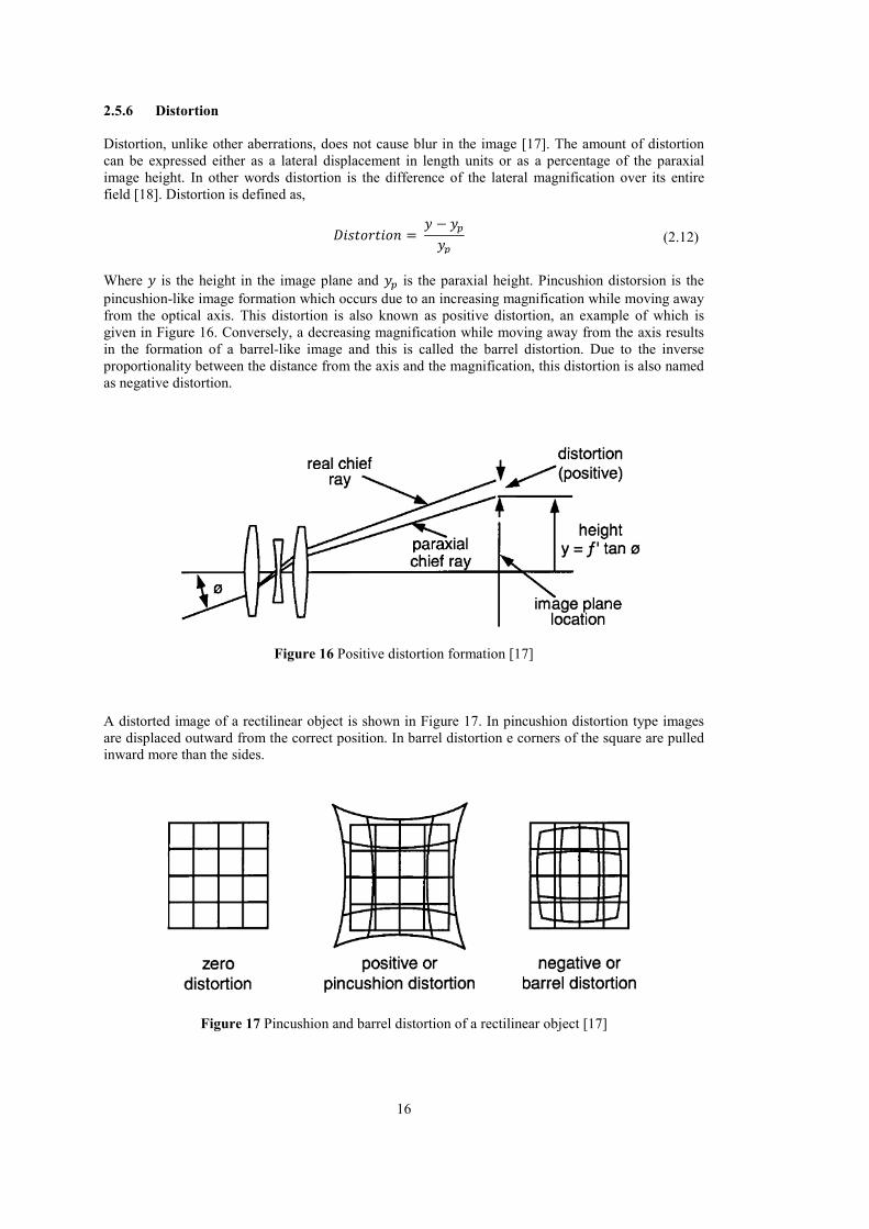
2.5.6 Distortion

Distortion, unlike other aberrations, does not cause blur in the image [17]. The amount of distortion can be expressed either as a lateral displacement in length units or as a percentage of the paraxial image height. In other words distortion is the difference of the lateral magnification over its entire field [18]. Distortion is defined as,

789:0-:80� = ; − ;<

;<

(2.12)

Where ; is the height in the image plane and ;< is the paraxial height. Pincushion distorsion is the

pincushion-like image formation which occurs due to an increasing magnification while moving away from the optical axis. This distortion is also known as positive distortion, an example of which is given in Figure 16. Conversely, a decreasing magnification while moving away from the axis results in the formation of a barrel-like image and this is called the barrel distortion. Due to the inverse proportionality between the distance from the axis and the magnification, this distortion is also named as negative distortion.

Figure 16 Positive distortion formation [17]

A distorted image of a rectilinear object is shown in Figure 17. In pincushion distortion type images are displaced outward from the correct position. In barrel distortion e corners of the square are pulled inward more than the sides.

Figure 17 Pincushion and barrel distortion of a rectilinear object [17]

17

Distortion is a cosmetic-type aberration that is not affecting resolution. Its occurrence is crucial especially in visual systems. While visually, 2% to 3% distortion is acceptable, it can be reduced to zero by appropriate stop position [17]. Lens thickness and position with respect to aperture stop designates its contribution to the distortion.

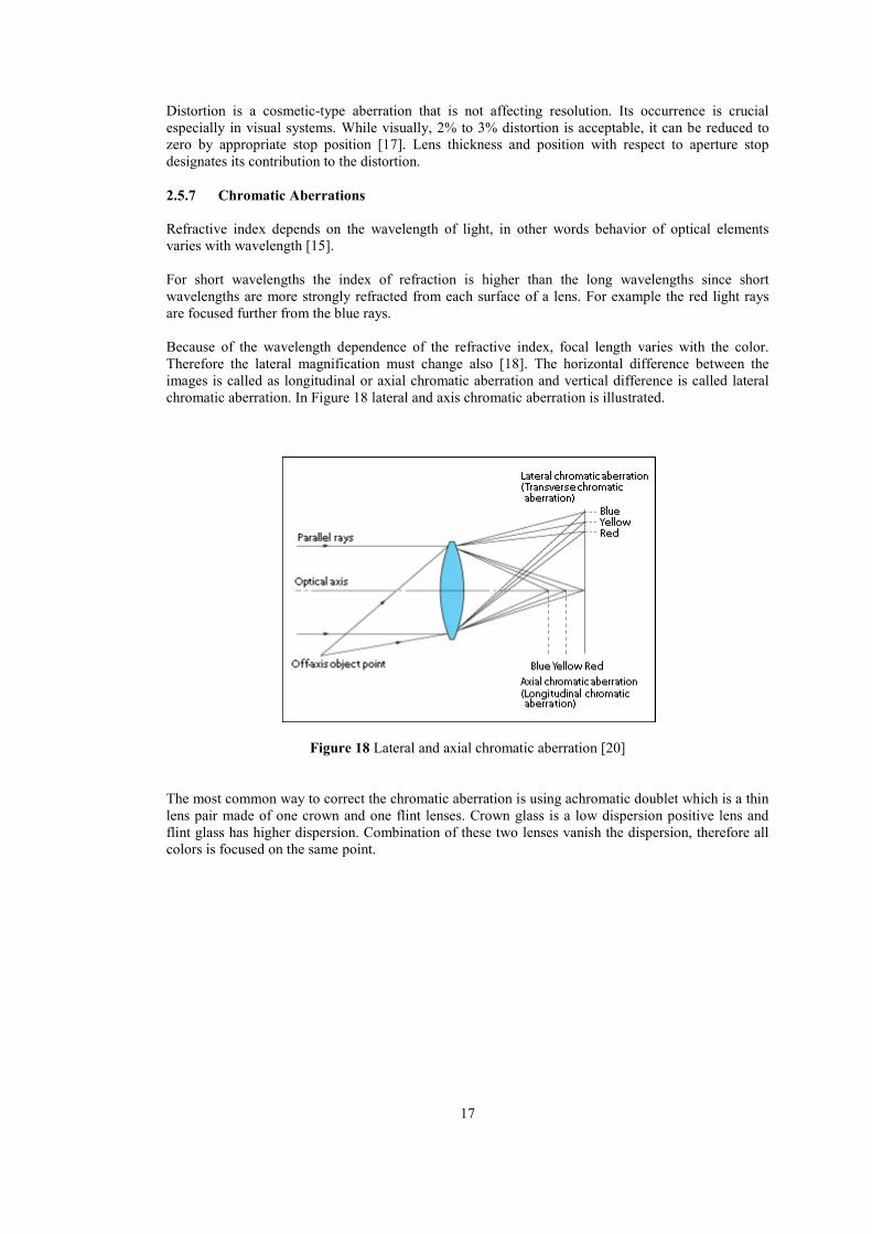
2.5.7 Chromatic Aberrations

Refractive index depends on the wavelength of light, in other words behavior of optical elements varies with wavelength [15]. For short wavelengths the index of refraction is higher than the long wavelengths since short wavelengths are more strongly refracted from each surface of a lens. For example the red light rays are focused further from the blue rays. Because of the wavelength dependence of the refractive index, focal length varies with the color. Therefore the lateral magnification must change also [18]. The horizontal difference between the images is called as longitudinal or axial chromatic aberration and vertical difference is called lateral chromatic aberration. In Figure 18 lateral and axis chromatic aberration is illustrated.

Figure 18 Lateral and axial chromatic aberration [20]

The most common way to correct the chromatic aberration is using achromatic doublet which is a thin lens pair made of one crown and one flint lenses. Crown glass is a low dispersion positive lens and flint glass has higher dispersion. Combination of these two lenses vanish the dispersion, therefore all colors is focused on the same point.

18

19

.

CHAPTER 3

OPTICAL METROLOGY TECHNOLOGIES

The study of expressing physical properties quantitatively through optical methods is called optical metrology [21]. In ‘‘Optical Metrology’’ the purpose is to measure some physical parameters using optical methods. Optical metrology generally deals with the measurements of length and straightness, angles between plane optical surfaces, surface quality of optical surfaces and curvature and focal length of lenses and mirrors. In this chapter curvature and surface quality measurement methods are described. There exist other alternative techniques for optical metrology measurement other than Hartmann sensors, some examples are interferometers, Foucault knife-edge test and curvature sensing [22]. In this chapter, a brief evaluation of Hartmann and other alternative techniques will be presented.

3.1 Interferometry

Interference is the situation of two waves combining to give a resultant wave of different amplitude. Superposition is applied in the interferometry calculations such that the combined wave carries the effects of originating waves. The combination of the waves of same frequency results in constructive interference in the case when they are in phase and vice versa when they are out of phase results in destructive interference [23].

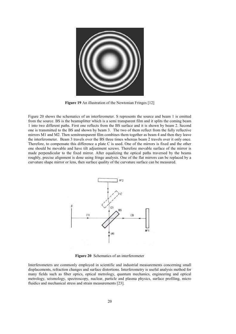
If two waves of the same frequency which are also in phase meet, the resultant magnitude is equal to the sum of each magnitude of the waves resulting in constructive interference. Similarly, if the waves which are of the same frequency and out of phase then the resultant magnitude is the difference of the magnitudes of the waves, resulting in the destructive interference. The Newtonian rings given in Figure 19 are examples for both the constructive and destructive interference resulting from the interference of the rays reflected from a spherical and a flat surface. Rings of light are the outcome of the constructive interference of the rays from the surfaces and the rings of dark regions are formed by destructive interference. Rings are replaced by some other shapes for surfaces that are not spherical.

20

Figure 19 An illustration of the Newtonian Fringes [12]

Figure 20 shows the schematics of an interferometer. S represents the source and beam 1 is emitted from the source. BS is the beamsplitter which is a semi transparent film and it splits the coming beam 1 into two different paths. First one reflects from the BS surface and it is shown by beam 2. Second one is transmitted to the BS and shown by beam 3. The two of them reflect from the fully reflective mirrors M1 and M2. Then semitransparent film combines them together as beam 4 and then they leave the interferometer. Beam 3 travels over the BS three times whereas beam 2 travels over it only once. Therefore, to compensate this difference a plate C is used. One of the mirrors is fixed and the other one should be movable and have tilt adjustment screws. Therefore movable surface of the mirror is made perpendicular to the fixed mirror. After equalizing the optical paths traversed by the beams roughly, precise alignment is done using fringe analysis. One of the flat mirrors can be replaced by a curvature shape mirror or lens, then surface quality of the curvature surface can be measured.

Figure 20 Schematics of an interferometer

Interferometers are commonly employed in scientific and industrial measurements concerning small displacements, refraction changes and surface distortions. Interferometry is useful analysis method for many fields such as fiber optics, optical metrology, quantum mechanics, engineering and optical metrology, seismology, spectroscopy, nuclear, particle and plasma physics, surface profiling, micro fluidics and mechanical stress and strain measurements [23].

21

Interferometry measurements are particularly useful for aberration measurements in high spatial frequency or low amplitude cases. However, some drawbacks exist about interferometers. For one, the measurement is very susceptible to environmental conditions such as air flow and mechanical vibrations especially while dealing with large beams. Also, to interpret and draw information from the measurements, complex software programs are required. An ordinary interferometer is quite expensive (around $100,000) in fact it is the most expensive among surface and curvature measurement alternatives.

3.2 Focault Knife Edge Test

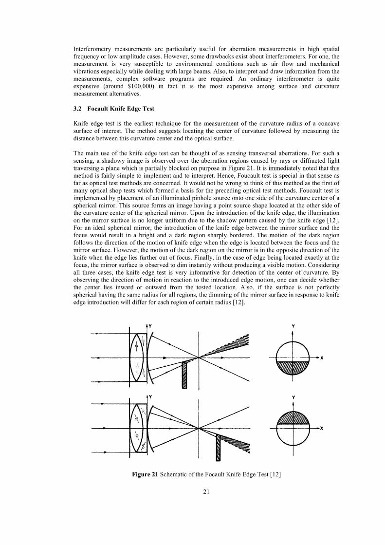
Knife edge test is the earliest technique for the measurement of the curvature radius of a concave surface of interest. The method suggests locating the center of curvature followed by measuring the distance between this curvature center and the optical surface. The main use of the knife edge test can be thought of as sensing transversal aberrations. For such a sensing, a shadowy image is observed over the aberration regions caused by rays or diffracted light traversing a plane which is partially blocked on purpose in Figure 21. It is immediately noted that this method is fairly simple to implement and to interpret. Hence, Foucault test is special in that sense as far as optical test methods are concerned. It would not be wrong to think of this method as the first of many optical shop tests which formed a basis for the preceding optical test methods. Foucault test is implemented by placement of an illuminated pinhole source onto one side of the curvature center of a spherical mirror. This source forms an image having a point source shape located at the other side of the curvature center of the spherical mirror. Upon the introduction of the knife edge, the illumination on the mirror surface is no longer uniform due to the shadow pattern caused by the knife edge [12]. For an ideal spherical mirror, the introduction of the knife edge between the mirror surface and the focus would result in a bright and a dark region sharply bordered. The motion of the dark region follows the direction of the motion of knife edge when the edge is located between the focus and the mirror surface. However, the motion of the dark region on the mirror is in the opposite direction of the knife when the edge lies further out of focus. Finally, in the case of edge being located exactly at the focus, the mirror surface is observed to dim instantly without producing a visible motion. Considering all three cases, the knife edge test is very informative for detection of the center of curvature. By observing the direction of motion in reaction to the introduced edge motion, one can decide whether the center lies inward or outward from the tested location. Also, if the surface is not perfectly spherical having the same radius for all regions, the dimming of the mirror surface in response to knife edge introduction will differ for each region of certain radius [12].

Figure 21 Schematic of the Focault Knife Edge Test [12]

22

In the case of multi-radius concave mirrors having different radius and center of curvature for different regions, a number of regions are dimmed upon the knife edge exertion. For a better understanding of the test scenario, one can think of the illumination source being on one side of the mirror and the knife edge being on the counter side of the mirror. Under such an illumination condition, regions having rising surface facing the source will be illuminated whereas the regions with falling surface will not get illumination or vice versa. In general, Foucault test is a useful method for the measurement of radius of curvature for different regions throughout the mirror surface and testing for the uniformity of the curvature radius over the entire spherical mirror. Past studies have shown that replacing the point source with a slit type of source does no harm to the Foucault test performance. The idea behind is that every point on the slit source forms identical images having the same shape and location with respect to the knife edge. These identical images add up to produce a large gain in the brightness of the image formed. However, for the assumption of identical image formation for all the points on the slit source to hold, the slit source must be oriented perfectly parallel to the knife edge. Only then the precision of the patterns can be maintained [12]. In summary, Foucault knife edge test makes use of a knife-edge moved through the focus of a beam. The result is obtained by the observation of the shadow patterns on the surface. Similar to interferometry, high spatial frequency aberrations can be detected by this method. However it must be noted that knife edge test necessities a precise alignment of the knife edge and the focus.

3.3 Curvature Sensing

Wavefront curvature sensing stands as a strong method with superior sensitivity, wide range and flexible spatial characteristics which make it a method of choice in various applications about optical metrology. Along with many benefits, curvature sensing also brings some difficulties. For instance, the intensity profile had to be measured for two separate planes along the optical axis which demanded a mechanical movement of optical parts or detector in the measurement. Such implementations rendered the wavefront sensing method as less stable when compared to other existing methods. However, with the introduction of new sensor designs capable of obtaining two separate images of the wavefront necessary for curvature sensing, the need for movement of the optical part is avoided while intensity profiles can be measured and analyzed [24]. Wavefront curvature sensors are used to measure the aberrations of an optical wavefront. In these sensors, an array of small lenses is used to focus the wavefront as an array of spots as in Shack-Hartmann wavefront sensors. Then the intensities on two sides of the focal plane are measured as opposed to the position measurement of the spots in Shack-Hartmann method [25]. The measurement of two intensities gives information about the curvature due to the fact that when a wavefront has phase curvature, it changes the focal spot position along the x-axis of the beam. Wavefront sensing has been an attraction for astronomical applications, laser beam profiling, adaptive optics, optical metrology and precision measurement of mechanical products in the industry. In adaptive optics, curvature sensing is commonly used to obtain the Laplacian of a wavefront by the difference of intensity profiles from points at equal distance on either side of the focus of a lens [22]. The intensity profiles of such two points are measured by mechanically moving some parts of the system which induces a substantial amount of noise to the system. Curvature sensing method has not been used commercially yet. This is the most important drawback of the method.

3.4 Shack Hartmann Method

Johannes Franz Hartmann is the inventor of Hartmann wavefront sensor which by the help of a bright

23

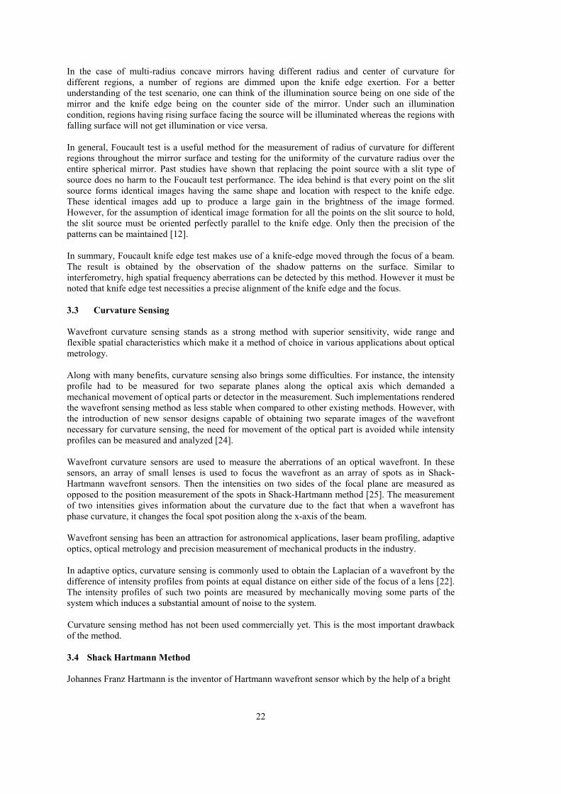
light source he first came up with when he managed to utilize the diffraction from an array of apertures through a sheet of metal to measure the impact of a test optic on the wavefront [22]. A screen having an array of holes is used in this method. This screen is placed near the entrance or exit pupil of the optical system to be tested. A typical screen can be seen in Figure 22 as a rectangular shaped array of holes one of which reside at the center location of the screen.

Figure 22 Hartmann test perspective schematics showing the Hartmann screen over a mirror to be tested [12]

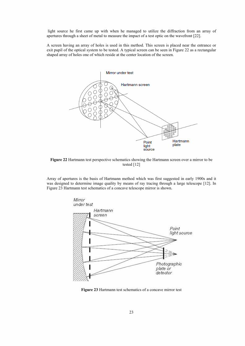
Array of apertures is the basis of Hartmann method which was first suggested in early 1900s and it was designed to determine image quality by means of ray tracing through a large telescope [12]. In Figure 23 Hartmann test schematics of a concave telescope mirror is shown.

Figure 23 Hartmann test schematics of a concave mirror test

24

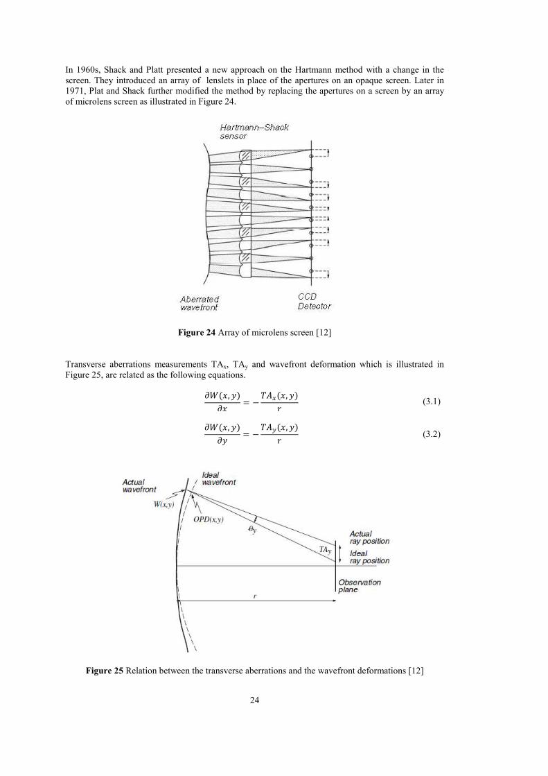
In 1960s, Shack and Platt presented a new approach on the Hartmann method with a change in the screen. They introduced an array of lenslets in place of the apertures on an opaque screen. Later in 1971, Plat and Shack further modified the method by replacing the apertures on a screen by an array of microlens screen as illustrated in Figure 24.

Figure 24 Array of microlens screen [12]

Transverse aberrations measurements TAx, TAy and wavefront deformation which is illustrated in Figure 25, are related as the following equations.

=>(?, ;)

=?= −

)*A(?, ;)

- (3.1)

=>(?, ;)

=;= −

)*B(?, ;)

- (3.2)

Figure 25 Relation between the transverse aberrations and the wavefront deformations [12]

25

In Figure 25, r is the distance between the pupil of the wavefront and the Hartmann plate. In the case of wavefront being convergent and Hartmann plate insides near the point of convergence, r becomes the radius of curvature for the wavefront. Figure 25 depicts wavefront aberration for the convergent wavefront case.

3.4.1 Functional Principle

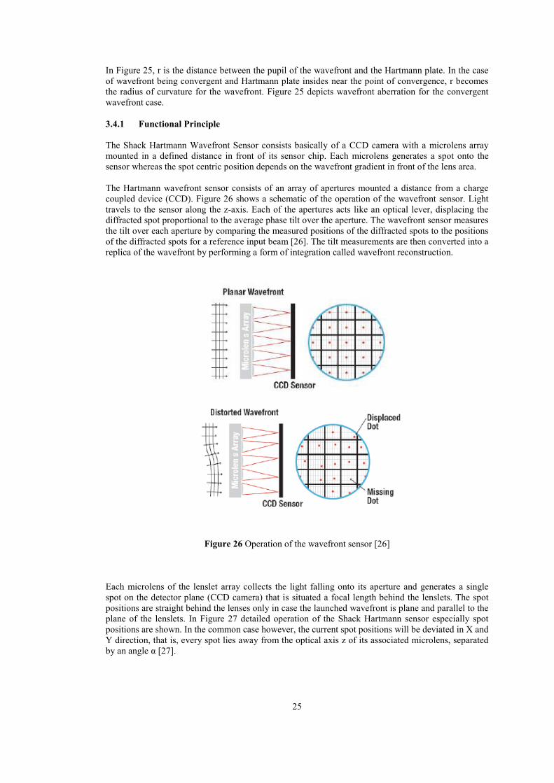
The Shack Hartmann Wavefront Sensor consists basically of a CCD camera with a microlens array mounted in a defined distance in front of its sensor chip. Each microlens generates a spot onto the sensor whereas the spot centric position depends on the wavefront gradient in front of the lens area. The Hartmann wavefront sensor consists of an array of apertures mounted a distance from a charge coupled device (CCD). Figure 26 shows a schematic of the operation of the wavefront sensor. Light travels to the sensor along the z-axis. Each of the apertures acts like an optical lever, displacing the diffracted spot proportional to the average phase tilt over the aperture. The wavefront sensor measures the tilt over each aperture by comparing the measured positions of the diffracted spots to the positions of the diffracted spots for a reference input beam [26]. The tilt measurements are then converted into a replica of the wavefront by performing a form of integration called wavefront reconstruction.

Figure 26 Operation of the wavefront sensor [26]

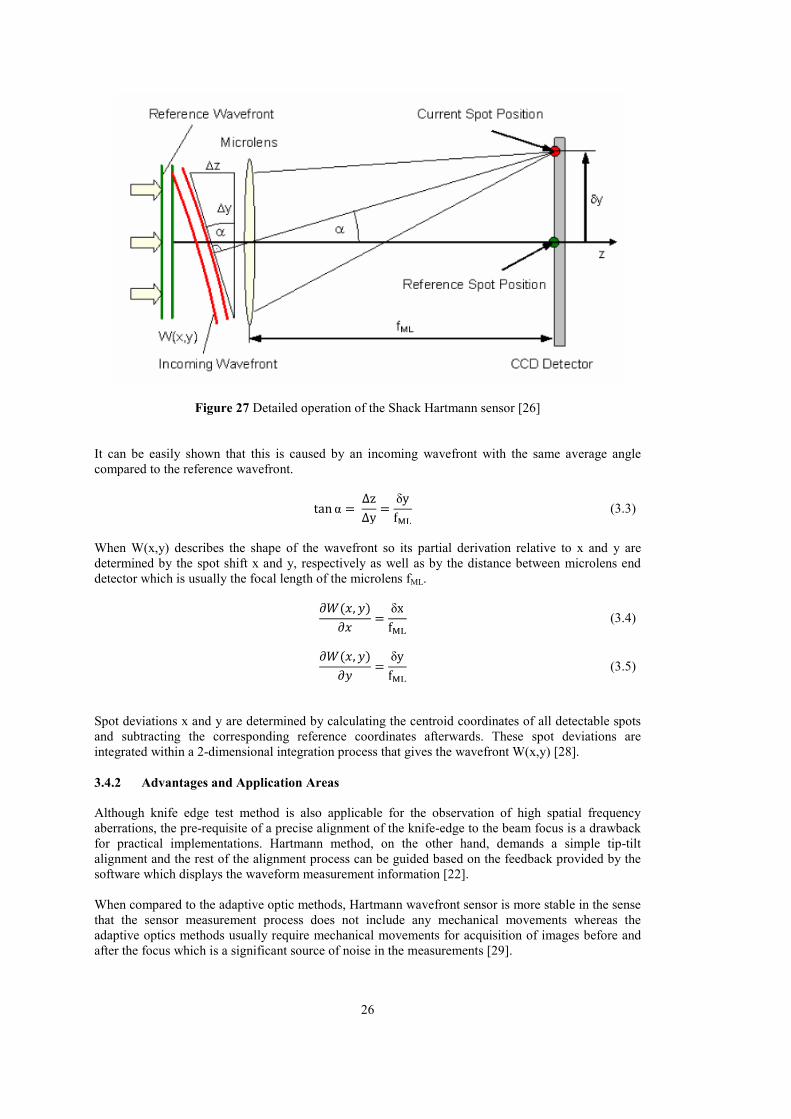
Each microlens of the lenslet array collects the light falling onto its aperture and generates a single spot on the detector plane (CCD camera) that is situated a focal length behind the lenslets. The spot positions are straight behind the lenses only in case the launched wavefront is plane and parallel to the plane of the lenslets. In Figure 27 detailed operation of the Shack Hartmann sensor especially spot positions are shown. In the common case however, the current spot positions will be deviated in X and Y direction, that is, every spot lies away from the optical axis z of its associated microlens, separated by an angle α [27].

26

Figure 27 Detailed operation of the Shack Hartmann sensor [26]

It can be easily shown that this is caused by an incoming wavefront with the same average angle compared to the reference wavefront.

tan α = ∆z

∆y=

δy

fGH

(3.3)

When W(x,y) describes the shape of the wavefront so its partial derivation relative to x and y are determined by the spot shift x and y, respectively as well as by the distance between microlens end detector which is usually the focal length of the microlens fML.

=>(?, ;)

=?=

δx

fGH

(3.4)

=>(?, ;)

=;=

δy

fGH

(3.5)

Spot deviations x and y are determined by calculating the centroid coordinates of all detectable spots and subtracting the corresponding reference coordinates afterwards. These spot deviations are integrated within a 2-dimensional integration process that gives the wavefront W(x,y) [28].

3.4.2 Advantages and Application Areas

Although knife edge test method is also applicable for the observation of high spatial frequency aberrations, the pre-requisite of a precise alignment of the knife-edge to the beam focus is a drawback for practical implementations. Hartmann method, on the other hand, demands a simple tip-tilt alignment and the rest of the alignment process can be guided based on the feedback provided by the software which displays the waveform measurement information [22]. When compared to the adaptive optic methods, Hartmann wavefront sensor is more stable in the sense that the sensor measurement process does not include any mechanical movements whereas the adaptive optics methods usually require mechanical movements for acquisition of images before and after the focus which is a significant source of noise in the measurements [29].

27

Hartmann wavefront sensor, unlike interferometers, can be insensitive to vibration by the removal of temporal noise through the use of averages of the frames. Hartmann sensor also provides simpler measurement interpretation as compared to the interferometers [30]. Furthermore, Hartmann wavefront sensors cost significantly less as compared to the typical cost of $100,000 for the interferometers. There are various methods of measuring wave-front aberrations; for example, the interferometric method, the Foucault knife-edge method, the Zernike filtering method, and so on. For measurements in real time, it seems most suitable to us to use a Hartmann sensor [5]. Shack-Hartmann sensor is an invention of 20th century which is a means of optical metrology. This sensor has been used in a wide range of applications some of which are adaptive optics (for satellite optics), ophthalmology (medical applications for human eye) and laser wavefront characterization.

28

29

….

CHAPTER 4

OPTICAL TEST SETUP DESIGN

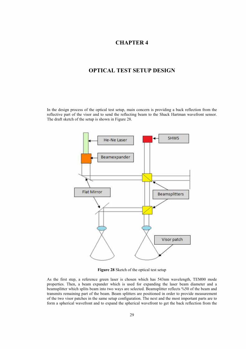
In the design process of the optical test setup, main concern is providing a back reflection from the reflective part of the visor and to send the reflecting beam to the Shack Hartman wavefront sensor. The draft sketch of the setup is shown in Figure 28.

Figure 28 Sketch of the optical test setup

As the first step, a reference green laser is chosen which has 543nm wavelength, TEM00 mode properties. Then, a beam expander which is used for expanding the laser beam diameter and a beamsplitter which splits beam into two ways are selected. Beamsplitter reflects %50 of the beam and transmits remaining part of the beam. Beam splitters are positioned in order to provide measurement of the two visor patches in the same setup configuration. The next and the most important parts are to form a spherical wavefront and to expand the spherical wavefront to get the back reflection from the

30

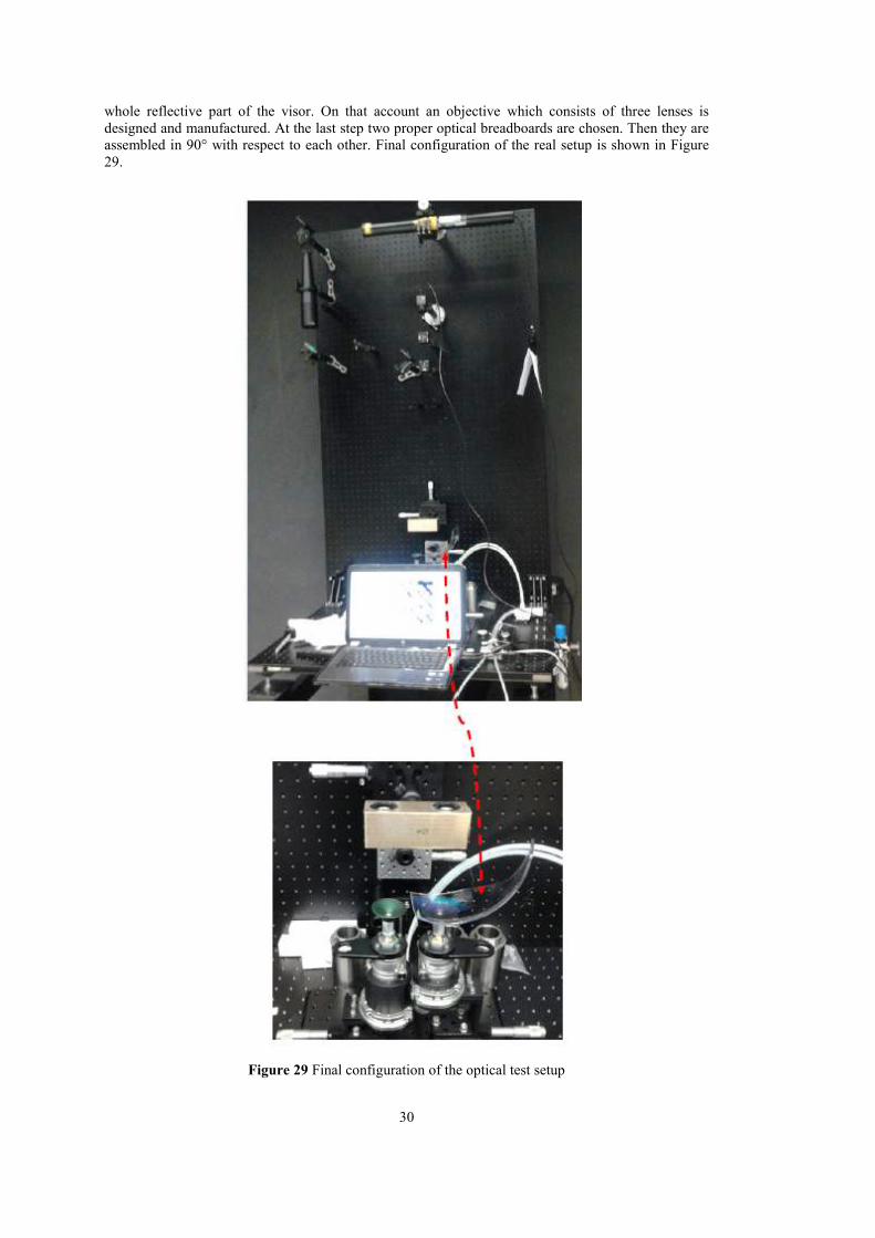
whole reflective part of the visor. On that account an objective which consists of three lenses is designed and manufactured. At the last step two proper optical breadboards are chosen. Then they are assembled in 90° with respect to each other. Final configuration of the real setup is shown in Figure 29.

Figure 29 Final configuration of the optical test setup

31

4.1 Optical Path Alignment

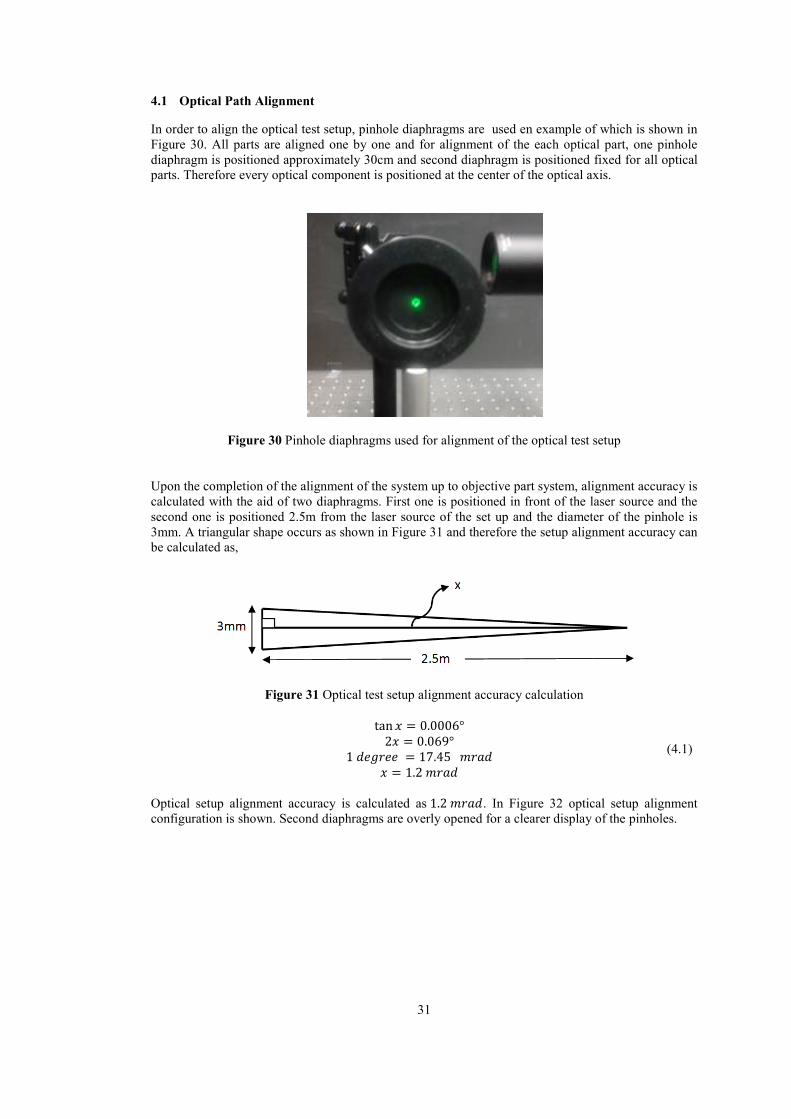
In order to align the optical test setup, pinhole diaphragms are used en example of which is shown in Figure 30. All parts are aligned one by one and for alignment of the each optical part, one pinhole diaphragm is positioned approximately 30cm and second diaphragm is positioned fixed for all optical parts. Therefore every optical component is positioned at the center of the optical axis.

Figure 30 Pinhole diaphragms used for alignment of the optical test setup

Upon the completion of the alignment of the system up to objective part system, alignment accuracy is calculated with the aid of two diaphragms. First one is positioned in front of the laser source and the second one is positioned 2.5m from the laser source of the set up and the diameter of the pinhole is 3mm. A triangular shape occurs as shown in Figure 31 and therefore the setup alignment accuracy can be calculated as,

Figure 31 Optical test setup alignment accuracy calculation

tan ? = 0.0006°

2? = 0.069°

1 MNO-NN = 17.45 1-2M

? = 1.2 1-2M

(4.1)

Optical setup alignment accuracy is calculated as 1.2 1-2M. In Figure 32 optical setup alignment configuration is shown. Second diaphragms are overly opened for a clearer display of the pinholes.

32

Figure 32 Optical test setup alignment configuration

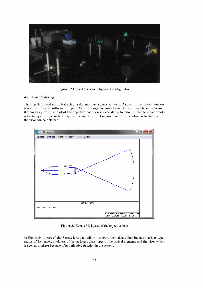
4.2 Lens Centering

The objective used in the test setup is designed via Zemax software. As seen in the layout window taken from Zemax software in Figure 33, this design consists of three lenses. Laser beam is focused 8.5mm away from the exit of the objective and then it expands up to visor surface to cover whole refractive part of the surface. By this means, wavefront measurements of the whole refractive part of the visor can be obtained.

.

Figure 33 Zemax 3D layout of the objective part

In Figure 34, a part of the Zemax lens data editor is shown. Lens data editor includes surface type, radius of the lenses, thickness of the surfaces, glass types of the optical elements and the visor which is seen as a mirror because of its reflective function in the system.

33

Figure 34 Zemax lens data editor of the objective design

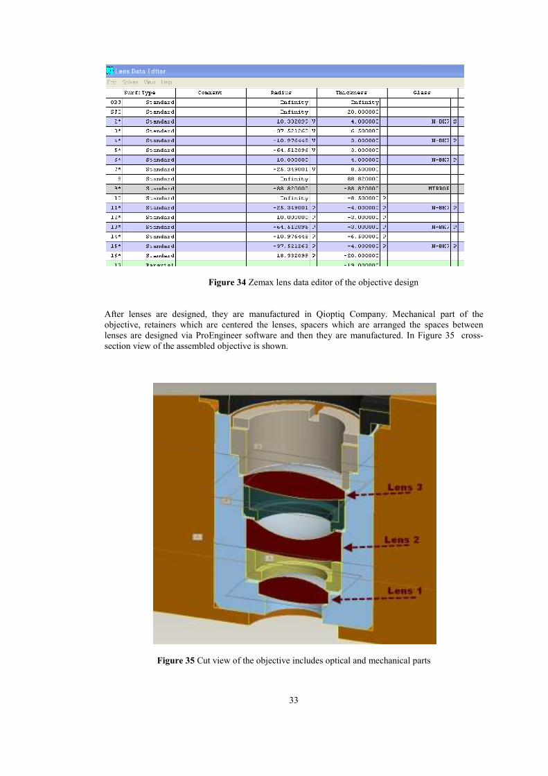
After lenses are designed, they are manufactured in Qioptiq Company. Mechanical part of the objective, retainers which are centered the lenses, spacers which are arranged the spaces between lenses are designed via ProEngineer software and then they are manufactured. In Figure 35 cross-section view of the assembled objective is shown.

Figure 35 Cut view of the objective includes optical and mechanical parts

34

The next step is to position the lenses into the mechanical part appropriately and then to measure the position error which gives informative results about the accuracy of the mechanical part of the objective.

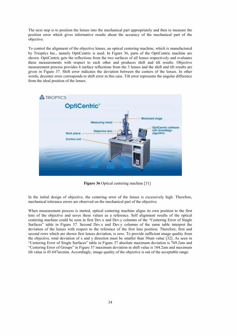
To control the alignment of the objective lenses, an optical centering machine, which is manufactured

by Trioptics Inc., namely OptiCentric is used. In Figure 36, parts of the OptiCentric machine are

shown. OptiCentric gets the reflections from the two surfaces of all lenses respectively and evaluates these measurements with respect to each other and produces shift and tilt results. Objective measurement process provides 6 surface reflections from the 3 lenses and the shift and tilt results are given in Figure 37. Shift error indicates the deviation between the centers of the lenses. In other words, decenter error corresponds to shift error in this case. Tilt error represents the angular difference from the ideal position of the lenses.

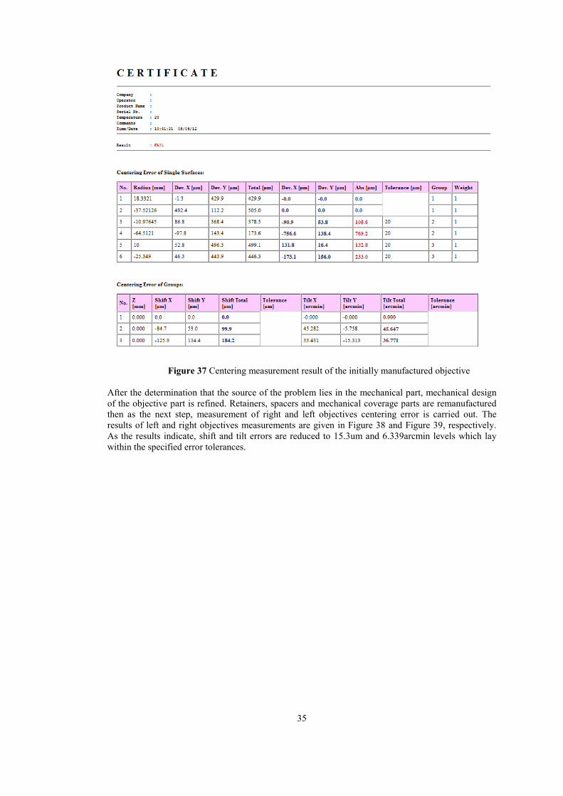
Figure 36 Optical centering machine [31]

In the initial design of objective, the centering error of the lenses is excessively high. Therefore, mechanical tolerance errors are observed on the mechanical part of the objective. When measurement process is started, optical centering machine aligns its own position to the first lens of the objective and saves these values as a reference. Self alignment results of the optical centering machine could be seen in first Dev.x and Dev.y columns of the “Centering Error of Single Surfaces” table in Figure 37. Second Dev.x and Dev.y columns of the same table interpret the deviation of the lenses with respect to the reference of the first lens position. Therefore, first and second rows which are shown first lenses deviation, is zero. To provide sufficient image quality from the objective, total deviation of x and y direction must be smaller than 50um value [32]. As seen in “Centering Error of Single Surfaces” table in Figure 37 absolute maximum deviation is 769.2um and “Centering Error of Groups” in Figure 37 maximum deviation in shift value is 184.2um and maximum tilt value is 45.647arcmin. Accordingly, image quality of the objective is out of the acceptable range.

35

Figure 37 Centering measurement result of the initially manufactured objective

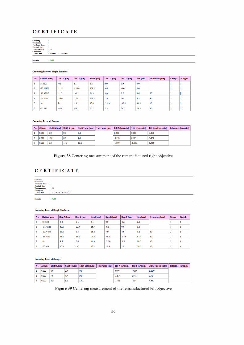
After the determination that the source of the problem lies in the mechanical part, mechanical design of the objective part is refined. Retainers, spacers and mechanical coverage parts are remanufactured then as the next step, measurement of right and left objectives centering error is carried out. The results of left and right objectives measurements are given in Figure 38 and Figure 39, respectively. As the results indicate, shift and tilt errors are reduced to 15.3um and 6.339arcmin levels which lay within the specified error tolerances.

36

Figure 38 Centering measurement of the remanufactured right objective

Figure 39 Centering measurement of the remanufactured left objective

37

4.3 5-DOF Holder for Visor

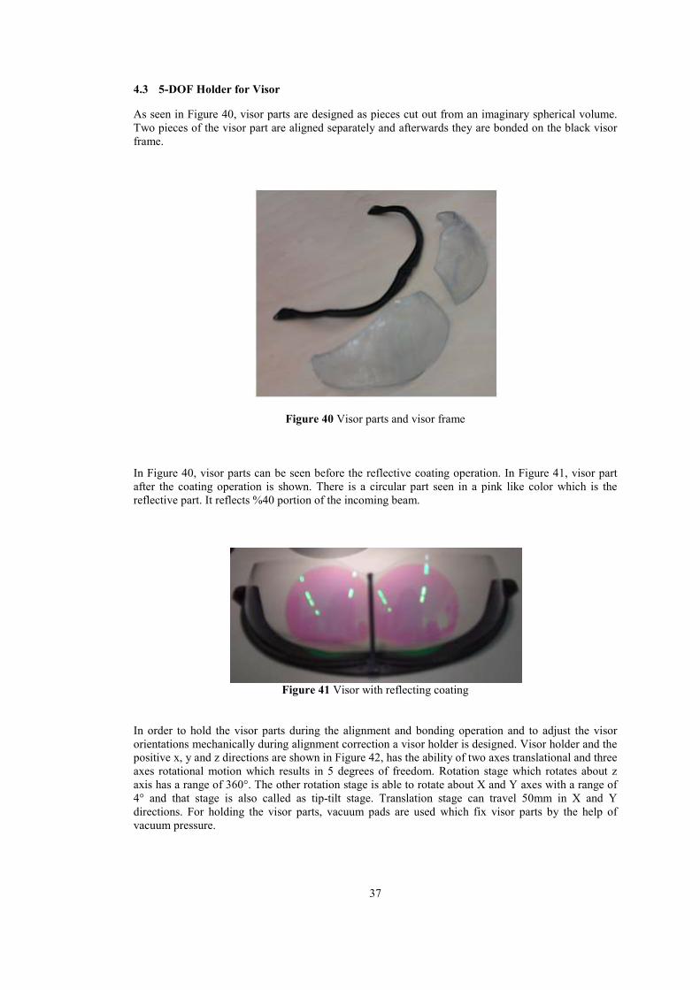
As seen in Figure 40, visor parts are designed as pieces cut out from an imaginary spherical volume. Two pieces of the visor part are aligned separately and afterwards they are bonded on the black visor frame.

Figure 40 Visor parts and visor frame

In Figure 40, visor parts can be seen before the reflective coating operation. In Figure 41, visor part after the coating operation is shown. There is a circular part seen in a pink like color which is the reflective part. It reflects %40 portion of the incoming beam.

Figure 41 Visor with reflecting coating

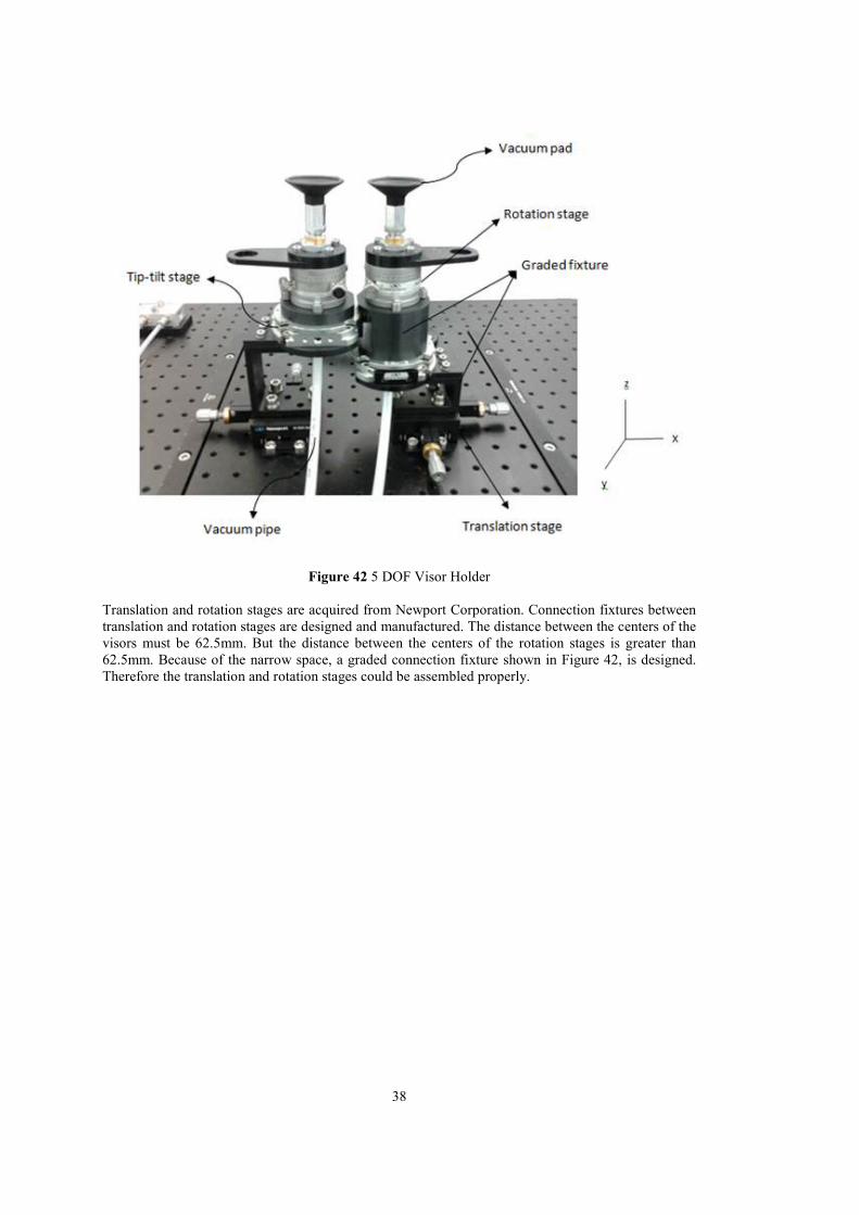
In order to hold the visor parts during the alignment and bonding operation and to adjust the visor orientations mechanically during alignment correction a visor holder is designed. Visor holder and the positive x, y and z directions are shown in Figure 42, has the ability of two axes translational and three axes rotational motion which results in 5 degrees of freedom. Rotation stage which rotates about z axis has a range of 360°. The other rotation stage is able to rotate about X and Y axes with a range of 4° and that stage is also called as tip-tilt stage. Translation stage can travel 50mm in X and Y directions. For holding the visor parts, vacuum pads are used which fix visor parts by the help of vacuum pressure.

38

Figure 42 5 DOF Visor Holder

Translation and rotation stages are acquired from Newport Corporation. Connection fixtures between translation and rotation stages are designed and manufactured. The distance between the centers of the visors must be 62.5mm. But the distance between the centers of the rotation stages is greater than 62.5mm. Because of the narrow space, a graded connection fixture shown in Figure 42, is designed. Therefore the translation and rotation stages could be assembled properly.

39

.

CHAPTER 5

ALIGNMENT METHOD

Optical setup provides the measurements to guide the alignment process. The wavefront measurement carries the information of how much the visors are optically aligned. In order to extract a measure of alignment and determine the actions to be taken to have the desired alignment, software guidance is needed. Shack-Hartmann sensor used in the optical setup provides Zernike coefficients calculated for the wavefront. When instantly observed from the measurement without a software interpretation, these coefficients give some hints about the misalignments, however, cannot describe the physical tilt and shift actions necessary to compensate the misalignments. Thus, if the software is created such that it can take the Zernike coefficients as inputs and give the existing misalignments in terms of tilt and shift values, then this information can be directly used to correct the alignment by applying the tilts and shifts to the holder of the visor. For this purpose, the first 9 terms of the Zernike coefficients provided by the wavefront sensor are determined as the input to the software and the tilts around X, Y axes and decenters along X, Y axes are the output of the software. As the Zernike coefficients are correlated, the most suitable way to map the input vector of dimension 9 to the output vector of dimension 4 is chosen as the artificial neural network approach. Neural network approach is a supervised method which requires sample data for training. For a satisfactory approximation of the input output relations, a sufficiently large number of training samples is needed. Such a large number of samples requires an automated data collection and leaves taking measurements by hand infeasible. Hence, the optical setup is modeled and simulated in the Zemax optical design program. In order to obtain the sample inputs and outputs, some certain tilts and decenters are induced on purpose and the behavior of corresponding Zernike coefficients in response to the applied misalignments are calculated and recorded by the Zemax program to text files. Then it is possible to find the necessary tilt/decenter movements to be applied to obtain alignment correction of the optical system. The overall procedure for the alignment correction method proposed is given in Figure 43.

5.1 Zemax Model of the Optical Test Setup Design

Zemax is a widely used optical design program. Analysis of optical systems can also be performed in Zemax. As a large number of sample measurements are needed for training the software design, it is not possible to iterate thousands of measurements in the real optical setup. Hence, the optical setup is simulated in Zemax environment, and by the help of macro code execution availability in Zemax,

hundreds of thousands of measurements are recorded automatically.

Zemax is conventional optical design software used for design and analysis of optical systems.

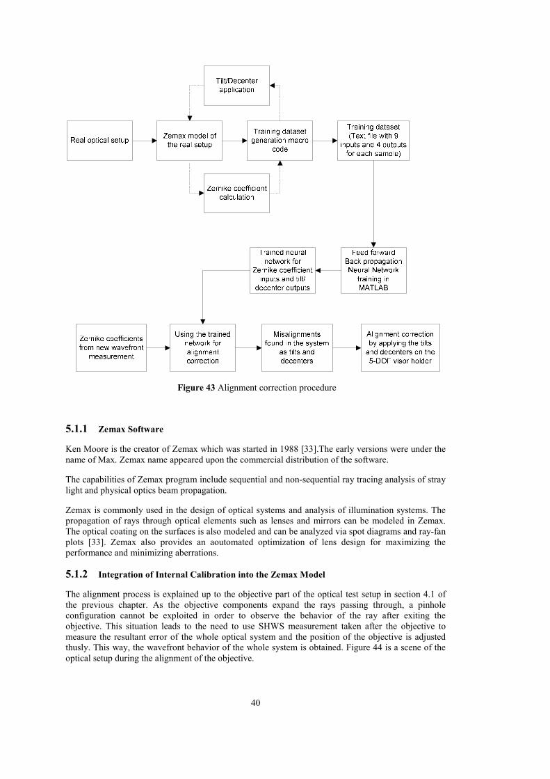
40

Figure 43 Alignment correction procedure

5.1.1 Zemax Software

Ken Moore is the creator of Zemax which was started in 1988 [33].The early versions were under the

name of Max. Zemax name appeared upon the commercial distribution of the software.

The capabilities of Zemax program include sequential and non-sequential ray tracing analysis of stray

light and physical optics beam propagation.

Zemax is commonly used in the design of optical systems and analysis of illumination systems. The propagation of rays through optical elements such as lenses and mirrors can be modeled in Zemax. The optical coating on the surfaces is also modeled and can be analyzed via spot diagrams and ray-fan plots [33]. Zemax also provides an aoutomated optimization of lens design for maximizing the performance and minimizing aberrations.

5.1.2 Integration of Internal Calibration into the Zemax Model

The alignment process is explained up to the objective part of the optical test setup in section 4.1 of the previous chapter. As the objective components expand the rays passing through, a pinhole configuration cannot be exploited in order to observe the behavior of the ray after exiting the objective. This situation leads to the need to use SHWS measurement taken after the objective to measure the resultant error of the whole optical system and the position of the objective is adjusted thusly. This way, the wavefront behavior of the whole system is obtained. Figure 44 is a scene of the

optical setup during the alignment of the objective.

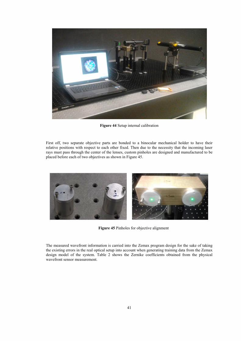
41

Figure 44 Setup internal calibration

First off, two separate objective parts are bonded to a binocular mechanical holder to have their relative positions with respect to each other fixed. Then due to the necessity that the incoming laser rays must pass through the center of the lenses, custom pinholes are designed and manufactured to be

placed before each of two objectives as shown in Figure 45.

Figure 45 Pinholes for objective alignment

The measured wavefront information is carried into the Zemax program design for the sake of taking the existing errors in the real optical setup into account when generating training data from the Zemax design model of the system. Table 2 shows the Zernike coefficients obtained from the physical

wavefront sensor measurement.

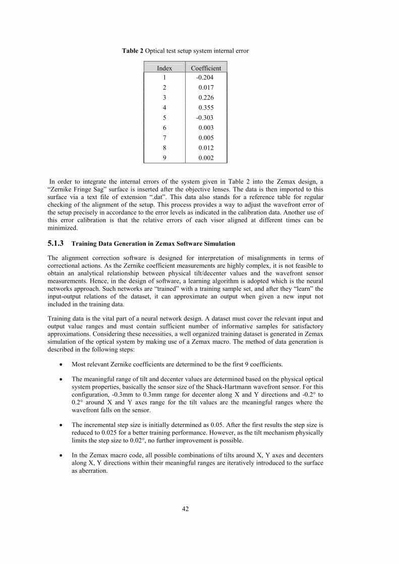
42

Table 2 Optical test setup system internal error

Index Coefficient

1 -0.204

2 0.017

3 0.226

4 0.355

5 -0.303

6 0.003

7 0.005

8 0.012

9 0.002

In order to integrate the internal errors of the system given in Table 2 into the Zemax design, a “Zernike Fringe Sag” surface is inserted after the objective lenses. The data is then imported to this surface via a text file of extension “.dat”. This data also stands for a reference table for regular checking of the alignment of the setup. This process provides a way to adjust the wavefront error of the setup precisely in accordance to the error levels as indicated in the calibration data. Another use of this error calibration is that the relative errors of each visor aligned at different times can be

minimized.

5.1.3 Training Data Generation in Zemax Software Simulation

The alignment correction software is designed for interpretation of misalignments in terms of correctional actions. As the Zernike coefficient measurements are highly complex, it is not feasible to obtain an analytical relationship between physical tilt/decenter values and the wavefront sensor measurements. Hence, in the design of software, a learning algorithm is adopted which is the neural networks approach. Such networks are “trained” with a training sample set, and after they “learn” the input-output relations of the dataset, it can approximate an output when given a new input not

included in the training data.

Training data is the vital part of a neural network design. A dataset must cover the relevant input and output value ranges and must contain sufficient number of informative samples for satisfactory approximations. Considering these necessities, a well organized training dataset is generated in Zemax simulation of the optical system by making use of a Zemax macro. The method of data generation is

described in the following steps:

• Most relevant Zernike coefficients are determined to be the first 9 coefficients.

• The meaningful range of tilt and decenter values are determined based on the physical optical system properties, basically the sensor size of the Shack-Hartmann wavefront sensor. For this configuration, -0.3mm to 0.3mm range for decenter along X and Y directions and -0.2° to 0.2° around X and Y axes range for the tilt values are the meaningful ranges where the

wavefront falls on the sensor.

• The incremental step size is initially determined as 0.05. After the first results the step size is reduced to 0.025 for a better training performance. However, as the tilt mechanism physically

limits the step size to 0.02°, no further improvement is possible.

• In the Zemax macro code, all possible combinations of tilts around X, Y axes and decenters along X, Y directions within their meaningful ranges are iteratively introduced to the surface

as aberration.

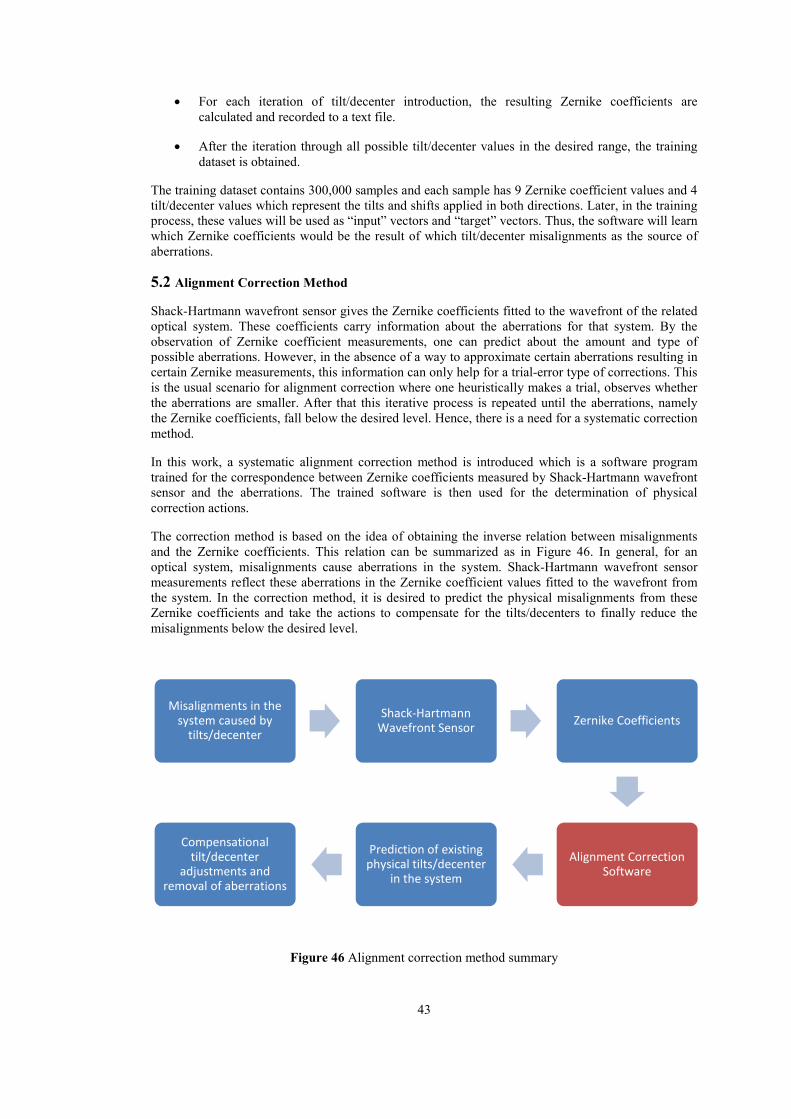
43

• For each iteration of tilt/decenter introduction, the resulting Zernike coefficients are

calculated and recorded to a text file.

• After the iteration through all possible tilt/decenter values in the desired range, the training

dataset is obtained.

The training dataset contains 300,000 samples and each sample has 9 Zernike coefficient values and 4 tilt/decenter values which represent the tilts and shifts applied in both directions. Later, in the training process, these values will be used as “input” vectors and “target” vectors. Thus, the software will learn which Zernike coefficients would be the result of which tilt/decenter misalignments as the source of

aberrations.

5.2 Alignment Correction Method

Shack-Hartmann wavefront sensor gives the Zernike coefficients fitted to the wavefront of the related optical system. These coefficients carry information about the aberrations for that system. By the observation of Zernike coefficient measurements, one can predict about the amount and type of possible aberrations. However, in the absence of a way to approximate certain aberrations resulting in certain Zernike measurements, this information can only help for a trial-error type of corrections. This is the usual scenario for alignment correction where one heuristically makes a trial, observes whether the aberrations are smaller. After that this iterative process is repeated until the aberrations, namely the Zernike coefficients, fall below the desired level. Hence, there is a need for a systematic correction

method.

In this work, a systematic alignment correction method is introduced which is a software program trained for the correspondence between Zernike coefficients measured by Shack-Hartmann wavefront sensor and the aberrations. The trained software is then used for the determination of physical

correction actions.

The correction method is based on the idea of obtaining the inverse relation between misalignments and the Zernike coefficients. This relation can be summarized as in Figure 46. In general, for an optical system, misalignments cause aberrations in the system. Shack-Hartmann wavefront sensor measurements reflect these aberrations in the Zernike coefficient values fitted to the wavefront from the system. In the correction method, it is desired to predict the physical misalignments from these Zernike coefficients and take the actions to compensate for the tilts/decenters to finally reduce the

misalignments below the desired level.

Figure 46 Alignment correction method summary

Misalignments in the system caused by

tilts/decenter

Shack-Hartmann Wavefront Sensor

Zernike Coefficients

Alignment Correction Software

Prediction of existing physical tilts/decenter

in the system

Compensational tilt/decenter

adjustments and removal of aberrations

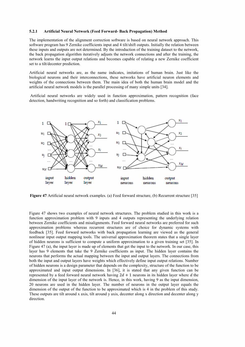
44

5.2.1 Artificial Neural Network (Feed Forward- Back Propagation) Method

The implementation of the alignment correction software is based on neural network approach. This software program has 9 Zernike coefficients input and 4 tilt/shift outputs. Initially the relation between these inputs and outputs are not determined. By the introduction of the training dataset to the network, the back propagation algorithm iteratively adjusts the network connections and after the training, the network learns the input output relations and becomes capable of relating a new Zernike coefficient

set to a tilt/decenter prediction.

Artificial neural networks are, as the name indicates, imitations of human brain. Just like the biological neurons and their interconnections, these networks have artificial neuron elements and weights of the connections between them. The main idea of both the human brain model and the

artificial neural network models is the parallel processing of many simple units [34].

Artificial neural networks are widely used in function approximation, pattern recognition (face

detection, handwriting recognition and so forth) and classification problems.

Figure 47 Artificial neural network examples. (a) Feed forward structure, (b) Recurrent structure [35]

Figure 47 shows two examples of neural network structures. The problem studied in this work is a function approximation problem with 9 inputs and 4 outputs representing the underlying relation between Zernike coefficients and misalignments. Feed forward neural networks are preferred for such approximation problems whereas recurrent structures are of choice for dynamic systems with feedback [35]. Feed forward networks with back propagation learning are viewed as the general nonlinear input output mapping tools. The universal approximation theorem states that a single layer of hidden neurons is sufficient to compute a uniform approximation to a given training set [35]. In Figure 47 (a), the input layer is made up of elements that get the input to the network. In our case, this layer has 9 elements that take the 9 Zernike coefficients as input. The hidden layer contains the neurons that performs the actual mapping between the input and output layers. The connections from both the input and output layers have weights which effectively define input output relations. Number of hidden neurons is a design parameter that depends on the complexity, structure of the function to be approximated and input output dimensions. In [36], it is stated that any given function can be

represented by a feed forward neural network having 2M + 1 neurons in its hidden layer where M the dimension of the input layer of the network is. Hence, in this work, having 9 as the input dimension, 20 neurons are used in the hidden layer. The number of neurons in the output layer equals the dimension of the output of the function to be approximated which is 4 in the problem of this study. These outputs are tilt around x axis, tilt around y axis, decenter along x direction and decenter along y

direction.

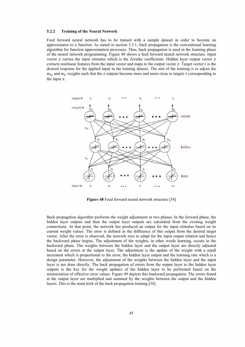
45

5.2.2 Training of the Neural Network

Feed forward neural network has to be trained with a sample dataset in order to become an approximator to a function. As stated in section 5.3.1, back propagation is the conventional learning algorithm for function approximation processes. Thus, back propagation is used in the learning phase of the neural network programming. Figure 48 shows a feed forward neural network structure. Input

vector ? carries the input stimulus which is the Zernike coefficients. Hidden layer output vector ;

extracts nonlinear features from the input vector and maps to the output vector P. Target vector : is the desired response for the applied input in the training dataset. The aim of the training is to adjust the

QRS and QS� weights such that the P outputs become more and more close to targets : corresponding to

the input ?.

Figure 48 Feed forward neural network structure [34]

Back propagation algorithm performs the weight adjustment in two phases. In the forward phase, the hidden layer outputs and then the output layer outputs are calculated from the existing weight connections. At that point, the network has produced an output for the input stimulus based on its current weight values. The error is defined as the difference of this output from the desired target vector. After the error is observed, the network tries to adapt for the input output relation and hence the backward phase begins. The adjustment of the weights, in other words learning, occurs in the backward phase. The weights between the hidden layer and the output layer are directly adjusted based on the errors at the output layer. The adjustment is the update of the weight with a small increment which is proportional to the error, the hidden layer output and the learning rate which is a design parameter. However, the adjustment of the weights between the hidden layer and the input layer is not done directly. The back propagation of errors from the output layer to the hidden layer outputs is the key for the weight updates of the hidden layer to be performed based on the minimization of effective error values. Figure 49 depicts this backward propagation. The errors found at the output layer are multiplied and summed by the weights between the output and the hidden

layers. This is the main trick of the back propagation training [34].

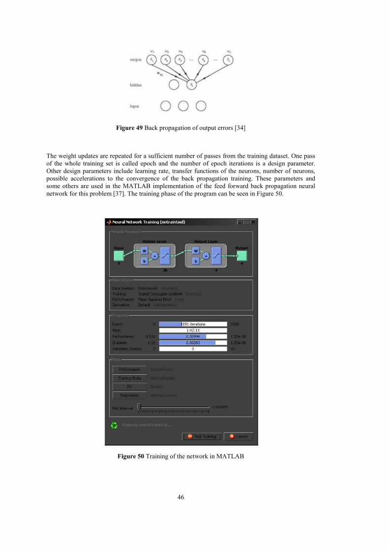
46

Figure 49 Back propagation of output errors [34]

The weight updates are repeated for a sufficient number of passes from the training dataset. One pass of the whole training set is called epoch and the number of epoch iterations is a design parameter. Other design parameters include learning rate, transfer functions of the neurons, number of neurons, possible accelerations to the convergence of the back propagation training. These parameters and some others are used in the MATLAB implementation of the feed forward back propagation neural

network for this problem [37]. The training phase of the program can be seen in Figure 50.

Figure 50 Training of the network in MATLAB

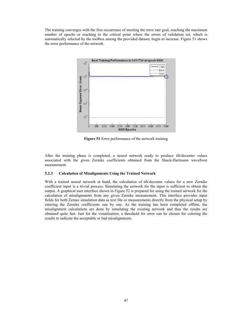
47

The training converges with the first occurrence of meeting the error rate goal, reaching the maximum number of epochs or reaching to the critical point where the errors of validation set, which is automatically selected by the toolbox among the provided dataset, begin to increase. Figure 51 shows

the error performance of the network.

Figure 51 Error performance of the network training

After the training phase is completed, a neural network ready to produce tilt/decenter values associated with the given Zernike coefficients obtained from the Shack-Hartmann wavefront

measurement.

5.2.3 Calculation of Misalignments Using the Trained Network

With a trained neural network at hand, the calculation of tilt/decenter values for a new Zernike coefficient input is a trivial process. Simulating the network for the input is sufficient to obtain the output. A graphical user interface shown in Figure 52 is prepared for using the trained network for the calculation of misalignments from any given Zernike measurement. This interface provides input fields for both Zemax simulation data as text file or measurements directly from the physical setup by entering the Zernike coefficients one by one. As the training has been completed offline, the misalignment calculations are done by simulating the existing network and thus the results are obtained quite fast. Just for the visualization, a threshold for error can be chosen for coloring the

results to indicate the acceptable or bad misalignments.

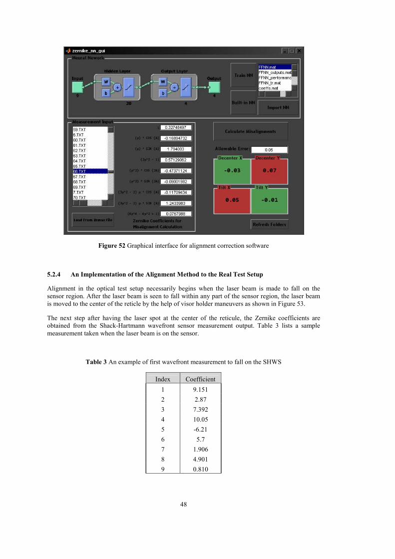
48

Figure 52 Graphical interface for alignment correction software

5.2.4 An Implementation of the Alignment Method to the Real Test Setup

Alignment in the optical test setup necessarily begins when the laser beam is made to fall on the sensor region. After the laser beam is seen to fall within any part of the sensor region, the laser beam is moved to the center of the reticle by the help of visor holder maneuvers as shown in Figure 53.

The next step after having the laser spot at the center of the reticule, the Zernike coefficients are obtained from the Shack-Hartmann wavefront sensor measurement output. Table 3 lists a sample

measurement taken when the laser beam is on the sensor.

Table 3 An example of first wavefront measurement to fall on the SHWS

Index Coefficient

1 9.151

2 2.87

3 7.392

4 10.05

5 -6.21

6 5.7

7 1.906

8 4.901

9 0.810

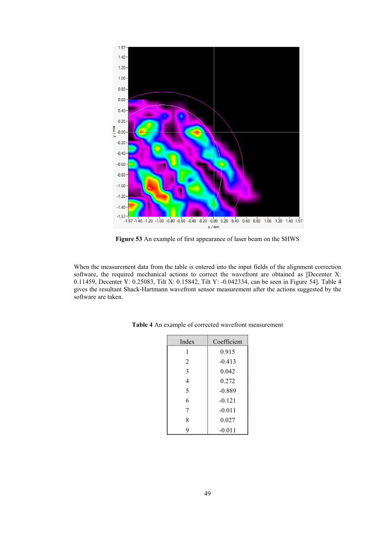
49

Figure 53 An example of first appearance of laser beam on the SHWS

When the measurement data from the table is entered into the input fields of the alignment correction software, the required mechanical actions to correct the wavefront are obtained as [Decenter X: 0.11459, Decenter Y: 0.25083, Tilt X: 0.15842, Tilt Y: -0.042334, can be seen in Figure 54]. Table 4 gives the resultant Shack-Hartmann wavefront sensor measurement after the actions suggested by the

software are taken.

Table 4 An example of corrected wavefront measurement

Index Coefficient

1 0.915

2 -0.413

3 0.042

4 0.272

5 -0.889

6 -0.121

7 -0.011

8 0.027

9 -0.011

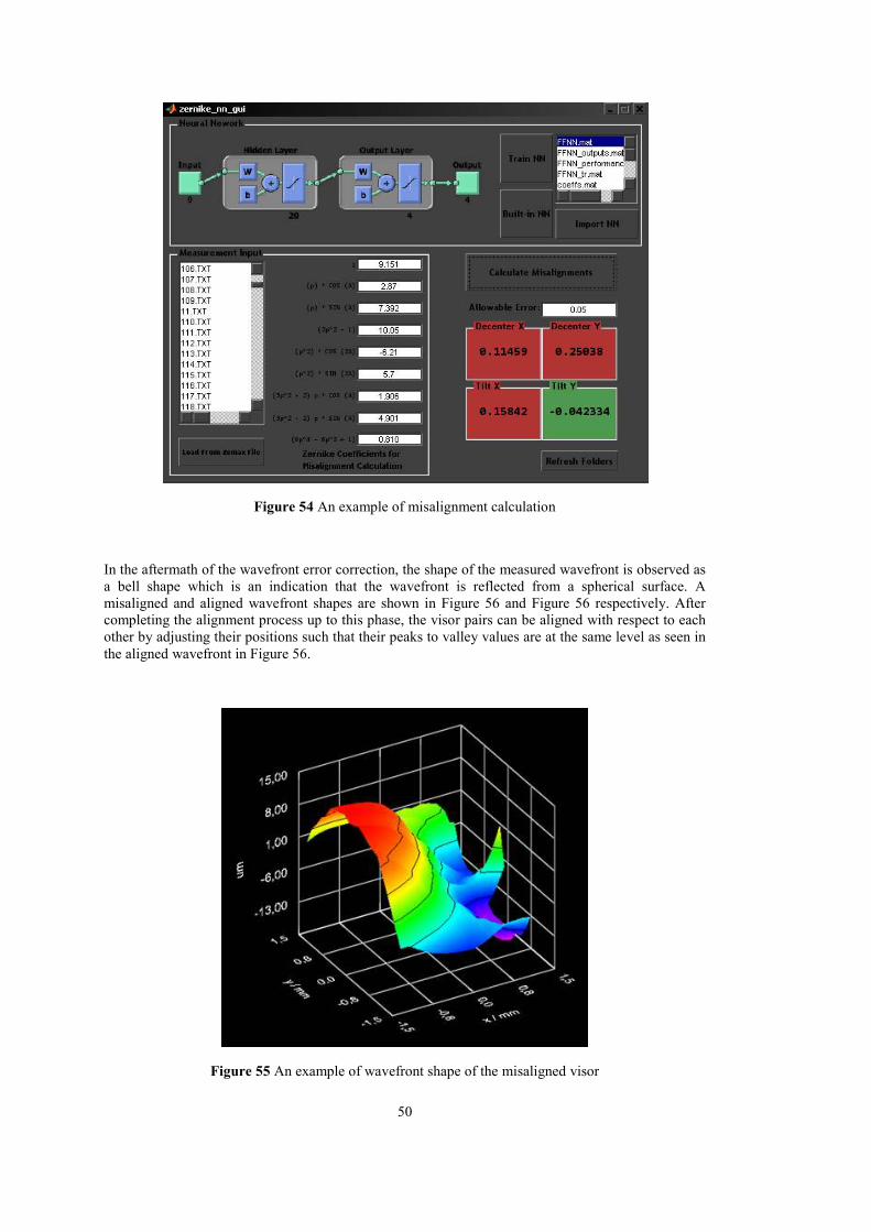
50

Figure 54 An example of misalignment calculation

In the aftermath of the wavefront error correction, the shape of the measured wavefront is observed as a bell shape which is an indication that the wavefront is reflected from a spherical surface. A misaligned and aligned wavefront shapes are shown in Figure 56 and Figure 56 respectively. After completing the alignment process up to this phase, the visor pairs can be aligned with respect to each other by adjusting their positions such that their peaks to valley values are at the same level as seen in

the aligned wavefront in Figure 56.

Figure 55 An example of wavefront shape of the misaligned visor

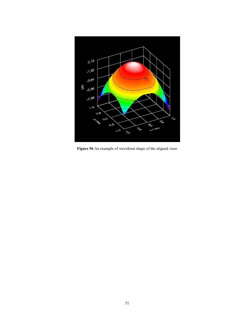
51

Figure 56 An example of wavefront shape of the aligned visor

52

53

..

CHAPTER 6

CONCLUSION

In this thesis, an optical alignment method for a spherical visor is investigated and a software solution is proposed for alignment correction. First, the aim of the study is expressed and the related part of the Aselsan Inc. project is briefly mentioned. The definition of the problem and a software based solution using the wavefront measurement are stated. The history of studies on the proposed method is mentioned. Before the implementation of the alignment procedure, the underlying aberration theory background is provided. The sources and types of aberrations are detailed. Zernike polynomials are introduced as a mathematical expression of aberrations. Optical metrology techniques are explained including the Shack-Hartmann method. The advantages and disadvantages of Shack-Hartmann method are discussed to explain why this method is chosen in this study. The operation principle of the Shack-Hartmann method is given in detail. Then, the design process of the optical test setup, the preferred components, the role of mechanical pin holes and modeling of the objective in the Zemax optical design program and finally the alignment by the use of the optical lens centering device are explained in detail. The complete operation principle of the optical setup is described in full detail. The final configuration of the optical setup and the solution algorithm based on the Zemax model of the system is presented. The study in the Optical Test Setup Design and Alignment Method chapters

can be outlined in the following headlines:

1. The construction of the optical setup and the alignment of the system up to the objective part

with an accuracy of 1.2mrad

2. The design of the optical and mechanical components of the objective

3. The alignment of lenses of the objective by using optical lens centering machine

4. Objective alignment with the optical setup by the help of pin holes designed for the

objectives

5. The measurement and the Zernike polynomial representation of the whole optical setup

wavefront error by making use of the Shack-Hartmann wavefront sensor

6. The integration of the measured wavefront errors into the Zemax optical design program

7. Training data generation by the help of a Zemax macro code and obtaining 300,000 data samples which contain wavefront error measurements resulting from the applied tilt and

decenter misalignments

8. The mapping of the 9 Zernike coefficients to the 4 tilt/decenter misalignments based on the

data samples generated in the Zemax model

9. The execution of the algorithm on the alignment of the optical setup and evaluation of results

obtained from experimental results

54

This study provides improvements on the alignment process by constructing software that guides through the physical adjustments of the visors. Compared to the traditional trial and error methods, significant amount of time is saved. Additionally, in most of the cases alignment with traditional methods is an unpredictable process which is not desirable for a time critical production line. The proposed alignment correction method enables alignment with the decenter errors along X and Y directions as 0.025mm and the tilt errors around X and Y axes as 0.025°. The sensitivity of tilt mechanism is a restraining factor for the tilt errors. Because the tilt mechanism having a range

between ±2° is not capable of micrometer scaling, it is not practical to apply small angle tilts.

The time consuming process of this study is the training data generation operation. The complete dataset generation takes days to finish on a workstation configuration computer. The most challenging phase of the study is the visor holder design process. In the test setup, two visors must be aligned separately but still consistent with respect to each other. This necessitates a 5 DOF holder for each visor at the same time which becomes very difficult as the visors are only 62.5mm apart from each other. This limits the workspace and a more accurate tilt mechanism of suitable size could not be

found.

Therefore, the first improvement for the future work will be a better suited visor holder. Two hexapods with suitable sizes to fit in 62.5mm spacing for the visors and having micrometer scale steps can be controlled by software incorporating with the alignment correction method. Projecting the laser beam onto the sensor region will be enough to have an automated alignment process. With this setup, the time span required for alignment and the final errors in the system can be further reduced. Also the accuracy of the tilt correction can be improved with highly sensitive incremental steps. When such a hexapod is available, the alignment correction software training part will be improved accordingly. The step size of training data sampling from Zemax software can be reduced for the sake of better sensitivity.

55

.

.REFERENCES

[1] Neal, D.R., Mansell, J., "Application of Shack-Hartmann Wavefront Sensors to Optical System

Calibration and Alignment," Stanford University Edward L. Ginzton Laboratory.

[2] M. Ruda, "Alignment of off-axis aspheric surfaces," SPIE, vol. 251, pp. 29-36, 1980.

[3] Liang,J., Grimm,B., Goelz,S., Bille,J.F., "Objective measurement of wave aberrations of the

human eye with the use of a Hartmann-Shack wave-front sensor," J.Opt. Soc. Am. A, vol. 11, no.

7, p. 1949, 1994.

[4] Forest,C. R., Canizares,C. R., Neal,D. R., McGuirk,M., Slocum,A.H., Schattenburg,M. L.,

"Metrology of Thin Transparent Optics Using Shack-Hartmann Wavefront Sensing," Optical

engineering, September 2003.

[5] Orlenko, E.A., Cherezova, T. Y., Sheldakova Y.V., Rukosuev, A. L., Kudryashov,A.V., "Off-

axis parabolic mirrors: A method of adjusting them and of measuring and correcting their

aberrations," Optical Society of America, no. 72, pp. 20-27, 2005.

[6] Baumhaker,H.,Witte,K.J.,Stehbeck,H., "Use of deformable mirrorsin theTI:S-laser ATLAS,"

Adaptive optics for Industry and Medicine, p. 28, 1999.

[7] Lundgren,M.A., Wolfe,W.L. , "Alignment of a three-mirror off-axis telescope by reverse

optimization," Optical Engineering, vol. 3, no. 30, pp. 307-311, 1991.

[8] Gao,Z., Chen,L., Zhou,S., Zhu,R., "Computer-aided alignment for a reference transmission

sphere of an interferometer," Society of Photo-Optical Instrumentation Engineers, 2004.

[9] "University of California, Center of Adaptive Optics," [Online]. Available:

http://cfao.ucolick.org/pubs/presentations/eyedesign. [Accessed 23 January 2013].

[10] Alda,J.,Arasa,J., "Paraxial Optics," Encyclopedia of Optical Engineering, 2004.

[11] Pedrotti,F.L.,Pedrotti,L.S., Introduction to Optics, New Jersey: Prentice-Hall, 1993.

[12] D. Malacara, Optical Shop Testing, Jhon Wiley & Sons, 2007.

[13] H. Gross, "Aberration Theory and Correction of Optical Systems," Handbook of Optical

Systems, vol. 3, 2007.

[14] V. Manajan, Aberration Theory Made Simple, SPIE Optical Engineering Press, 1991.

[15] W. Smith, Modern Optical Engineering, Mc Graw-Hill, 2000.

56

[16] "Photoplaza," [Online]. Available: http://www.photoplaza.nl. [Accessed 14 January 2013].

[17] Fisher,R.E.,Biljana,T.G., Optical System Design, SPIE Press-McGrawhil, 2000.

[18] Jenkis,F.A.,White,H.E., Fundamentals of Optics, Mc Graw-Hill, 1957.

[19] "Hyperphysics," [Online]. Available: http://hyperphysics.phy-astr.gsu.edu . [Accessed 3

December 2012].

[20] "Canon corporation," [Online]. Available: http://www.canon.com/cameramuseum/tech/report/.

[Accessed 7 January 2013].

[21] H. Stahl, " Rules for Optical Metrology," International Commission for Optic 22nd General

Congress, vol. 22, 2011.

[22] Spiricon, "Hartmann Wavefront Analyzer Tutorial," Spiricon, Inc., Utah, 2004.

[23] P. Hariharan, Basics of Interferometry, Elsevier Inc., 2007.

[24] D. Robinson, "Wavefront Curvature sensor Technology and Application to Optical Metrology,"

Arden Photonics, 2004.

[25] R. François, "Curvature sensing and compensation: a new concept in adaptive optics,," 1988.

[26] Thorlabs, "Operation Manual Optical Wavefront Sensor,WFS150-5C," Thorlabs

Instrumentation.

[27] R. Shack, "Production and use of alenticular Hartmann screen," Optical Soc. Am., vol. 61, p. 656,

1971.

[28] Curatu,C.,Curatu,G.,Rolland,J., "Tolerance analysis method for Shack-Hartmann sensors using a

variable phase surface," Optical Society of America, vol. 14, p. 138.

[29] Fund,J.P.,Lindlein,Schwider,J., "Misalignment effects of the Shack Hartmann Sensor," Optics

InfoBase, vol. 37, no. 1, p. 22, 1998.

[30] Su,P.,Parks,R.E.,Wang,L.,Angel,R.P.,Burge,J.H., "Software configurable optical test system:a

computerized reverse Hartmann test," Optics InfoBase, vol. 49, no. 23, p. 4404, 2010.

[31] "Trioptics," [Online]. Available: http://www.trioptics.com/pdfs/OptiCentric_E_2010_web.pdf.

[Accessed 15 December 2012].

[32] G. Curatu, " Tolerances in Optical Design,Orlando 2010)," LensAR Inc., Orlando, 2010.

[33] K. Moore, "Radiantzemax," [Online]. Available: http://www.radiantzemax.com/kb-

en/KnowledgebaseArticle.aspx . [Accessed 27 December 2012].

[34] Duda,R.O., Stork,P.E.,Hart,D.G., Pattern Classification, Wiley Interscience,, 2001.

57

[35] S. Haykin, Neural Networks, A Comprehensive Foundation, Prentice Hall, 1999.

[36] A. Kolmogorov, "On the Representation of Continuous Functions of Several Variables by

Superposition of Continuous Functions of one Variable and Addition," Doklady Akademii, vol.

114, pp. 679-681, 1957.

[37] M. H. Beale, M. T. Hagan, H. B. Demuth, "[MATLAB Neural Network Toolbox User’s Guide,

M. H. BealeMATLAB Neural Network Toolbox User’s Guide," MathWorks Inc, 2012.

[38] "Thorlabs," [Online]. Available:

http://www.thorlabs.com/newgrouppage9.cfm?objectgroup_id=2946. [Accessed 3 January

2013].

58

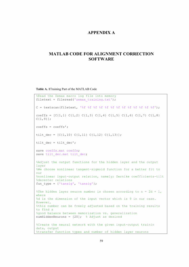
59

.

APPENDIX A

MATLAB CODE FOR ALIGNMENT CORRECTION

SOFTWARE

Table A. 1Training Part of the MATLAB Code

%Read the Zemax macro log file into memory filetext = fileread('zemax_training.txt'); C = textscan(filetext, '%f %f %f %f %f %f %f %f %f %f %f %f %f'); coeffs = [C{1,1} C{1,2} C{1,3} C{1,4} C{1,5} C{1,6} C{1,7} C{1,8} C{1,9}]; coeffs = coeffs'; tilt_dec = [C{1,10} C{1,11} C{1,12} C{1,13}]; tilt_dec = tilt_dec'; save coeffs.mat coeffs; save tilt_dec.mat tilt_dec; %Adjust the output functions for the hidden layer and the output layer %We choose nonlinear tangent-sigmoid function for a better fit to our %nonlinear input-output relation, namely; Zernike coefficients-tilt %decenter relations fun_type = {'tansig', 'tansig'}; %The hidden layer neuron number is chosen according to n = 2d + 1, where %d is the dimension of the input vector which is 9 in our case. However, %this number can be freely adjusted based on the training results to find a %good balance between memorization vs. generalization numHiddenNeurons = [20]; % Adjust as desired %Create the neural network with the given input-output trainin data, output %transfer function types and number of hidden layer neurons

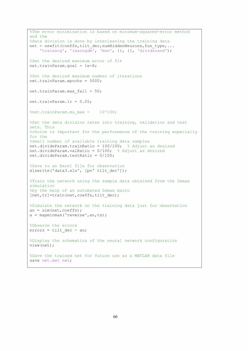
60

%The error minimization is based on minimum-squared-error method and the %data division is done by interleaving the training data net = newfit(coeffs,tilt_dec,numHiddenNeurons,fun_type,... 'trainscg', 'learngdm', 'mse', {}, {}, 'dividerand'); %Set the desired maximum error of fit net.trainParam.goal = 1e-8; %Set the desired maximum number of iterations net.trainParam.epochs = 5000; net.trainParam.max_fail = 50; net.trainParam.lr = 0.05; %net.trainParam.mu_max = 10^100; %Set the data division rates into training, validation and test sets. This %choice is important for the performance of the training especially for the %small number of available training data samples net.divideParam.trainRatio = 100/100; % Adjust as desired net.divideParam.valRatio = 0/100; % Adjust as desired net.divideParam.testRatio = 0/100; %Save to an Excel file for observation xlswrite('data3.xls', [pn' tilt_dec']);

%Train the network using the sample data obtained from the Zemax simulation %by the help of an automated Zemax macro [net,tr]=train(net,coeffs,tilt_dec); %Simulate the network on the training data just for observation an = sim(net,coeffs); a = mapminmax('reverse',an,ts);

%Observe the errors errors = tilt_dec - an;

%Display the schematics of the neural network configuration view(net); %Save the trained net for future use as a MATLAB data file save net.mat net;

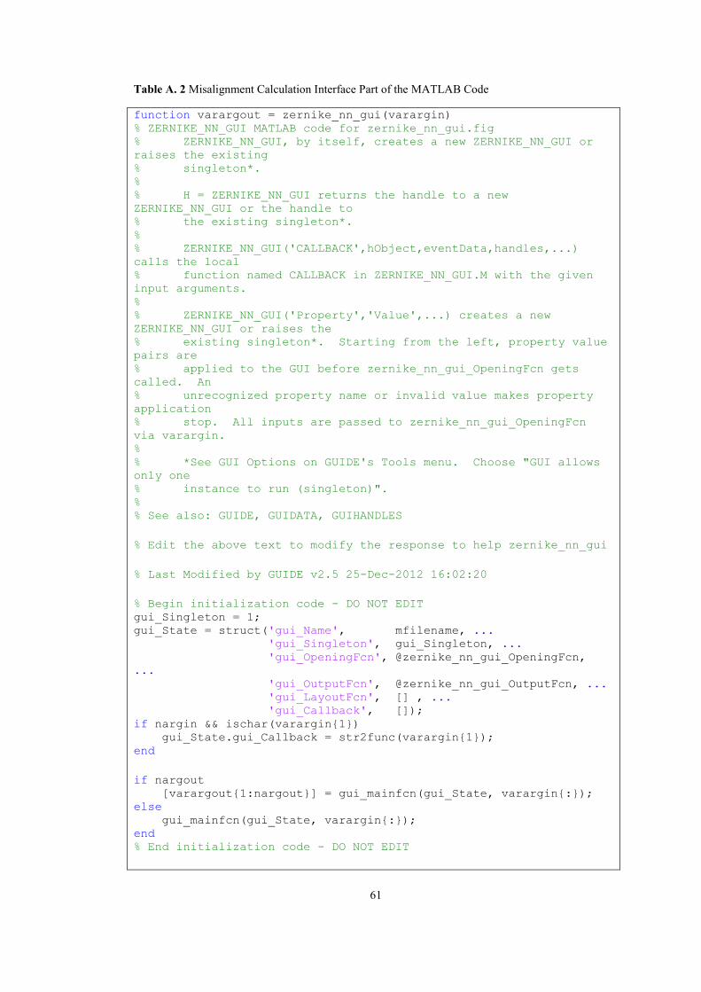
61

Table A. 2 Misalignment Calculation Interface Part of the MATLAB Code

function varargout = zernike_nn_gui(varargin) % ZERNIKE_NN_GUI MATLAB code for zernike_nn_gui.fig % ZERNIKE_NN_GUI, by itself, creates a new ZERNIKE_NN_GUI or raises the existing % singleton*. % % H = ZERNIKE_NN_GUI returns the handle to a new ZERNIKE_NN_GUI or the handle to % the existing singleton*. % % ZERNIKE_NN_GUI('CALLBACK',hObject,eventData,handles,...) calls the local % function named CALLBACK in ZERNIKE_NN_GUI.M with the given input arguments. % % ZERNIKE_NN_GUI('Property','Value',...) creates a new ZERNIKE_NN_GUI or raises the % existing singleton*. Starting from the left, property value pairs are % applied to the GUI before zernike_nn_gui_OpeningFcn gets called. An % unrecognized property name or invalid value makes property application % stop. All inputs are passed to zernike_nn_gui_OpeningFcn via varargin. % % *See GUI Options on GUIDE's Tools menu. Choose "GUI allows only one % instance to run (singleton)". % % See also: GUIDE, GUIDATA, GUIHANDLES % Edit the above text to modify the response to help zernike_nn_gui % Last Modified by GUIDE v2.5 25-Dec-2012 16:02:20 % Begin initialization code - DO NOT EDIT gui_Singleton = 1; gui_State = struct('gui_Name', mfilename, ... 'gui_Singleton', gui_Singleton, ... 'gui_OpeningFcn', @zernike_nn_gui_OpeningFcn, ... 'gui_OutputFcn', @zernike_nn_gui_OutputFcn, ... 'gui_LayoutFcn', [] , ... 'gui_Callback', []); if nargin && ischar(varargin{1}) gui_State.gui_Callback = str2func(varargin{1}); end if nargout [varargout{1:nargout}] = gui_mainfcn(gui_State, varargin{:}); else gui_mainfcn(gui_State, varargin{:}); end % End initialization code - DO NOT EDIT

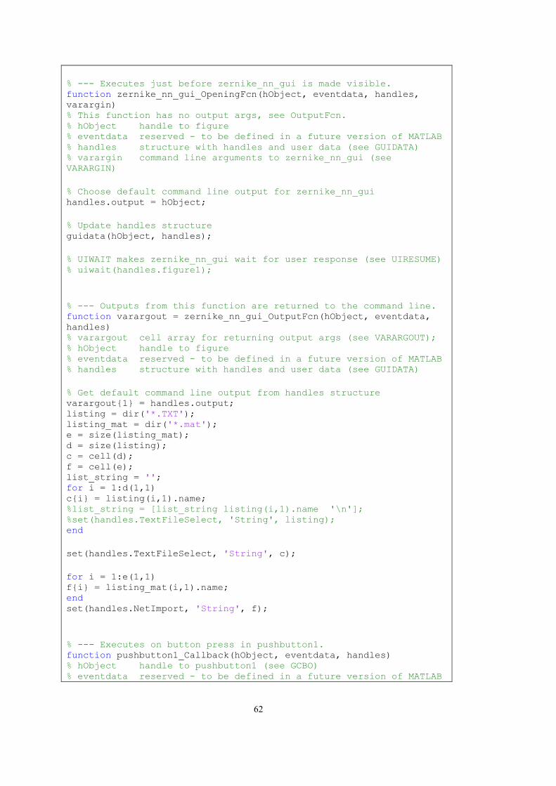
62

% --- Executes just before zernike_nn_gui is made visible. function zernike_nn_gui_OpeningFcn(hObject, eventdata, handles, varargin) % This function has no output args, see OutputFcn. % hObject handle to figure % eventdata reserved - to be defined in a future version of MATLAB % handles structure with handles and user data (see GUIDATA) % varargin command line arguments to zernike_nn_gui (see VARARGIN) % Choose default command line output for zernike_nn_gui handles.output = hObject; % Update handles structure guidata(hObject, handles); % UIWAIT makes zernike_nn_gui wait for user response (see UIRESUME) % uiwait(handles.figure1); % --- Outputs from this function are returned to the command line. function varargout = zernike_nn_gui_OutputFcn(hObject, eventdata, handles) % varargout cell array for returning output args (see VARARGOUT); % hObject handle to figure % eventdata reserved - to be defined in a future version of MATLAB % handles structure with handles and user data (see GUIDATA) % Get default command line output from handles structure varargout{1} = handles.output; listing = dir('*.TXT'); listing_mat = dir('*.mat'); e = size(listing_mat); d = size(listing); c = cell(d); f = cell(e); list_string = ''; for i = 1:d(1,1) c{i} = listing(i,1).name; %list_string = [list_string listing(i,1).name '\n']; %set(handles.TextFileSelect, 'String', listing); end set(handles.TextFileSelect, 'String', c); for i = 1:e(1,1) f{i} = listing_mat(i,1).name; end set(handles.NetImport, 'String', f); % --- Executes on button press in pushbutton1. function pushbutton1_Callback(hObject, eventdata, handles) % hObject handle to pushbutton1 (see GCBO) % eventdata reserved - to be defined in a future version of MATLAB

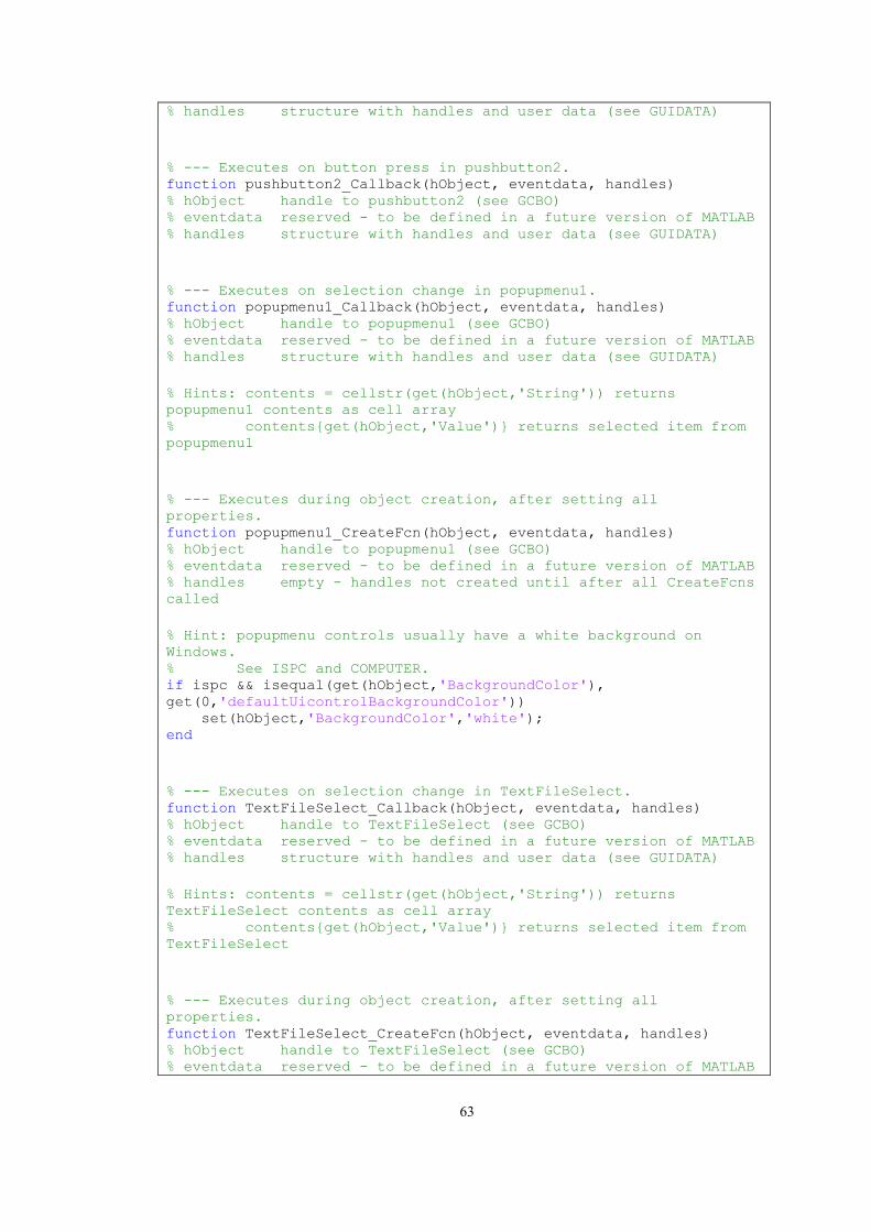
63

% handles structure with handles and user data (see GUIDATA) % --- Executes on button press in pushbutton2. function pushbutton2_Callback(hObject, eventdata, handles) % hObject handle to pushbutton2 (see GCBO) % eventdata reserved - to be defined in a future version of MATLAB % handles structure with handles and user data (see GUIDATA) % --- Executes on selection change in popupmenu1. function popupmenu1_Callback(hObject, eventdata, handles) % hObject handle to popupmenu1 (see GCBO) % eventdata reserved - to be defined in a future version of MATLAB % handles structure with handles and user data (see GUIDATA) % Hints: contents = cellstr(get(hObject,'String')) returns popupmenu1 contents as cell array % contents{get(hObject,'Value')} returns selected item from popupmenu1 % --- Executes during object creation, after setting all properties. function popupmenu1_CreateFcn(hObject, eventdata, handles) % hObject handle to popupmenu1 (see GCBO) % eventdata reserved - to be defined in a future version of MATLAB % handles empty - handles not created until after all CreateFcns called % Hint: popupmenu controls usually have a white background on Windows. % See ISPC and COMPUTER. if ispc && isequal(get(hObject,'BackgroundColor'), get(0,'defaultUicontrolBackgroundColor')) set(hObject,'BackgroundColor','white'); end % --- Executes on selection change in TextFileSelect. function TextFileSelect_Callback(hObject, eventdata, handles) % hObject handle to TextFileSelect (see GCBO) % eventdata reserved - to be defined in a future version of MATLAB % handles structure with handles and user data (see GUIDATA) % Hints: contents = cellstr(get(hObject,'String')) returns TextFileSelect contents as cell array % contents{get(hObject,'Value')} returns selected item from TextFileSelect % --- Executes during object creation, after setting all properties. function TextFileSelect_CreateFcn(hObject, eventdata, handles) % hObject handle to TextFileSelect (see GCBO) % eventdata reserved - to be defined in a future version of MATLAB

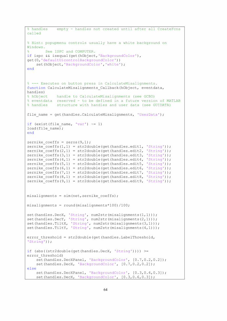
64

% handles empty - handles not created until after all CreateFcns called % Hint: popupmenu controls usually have a white background on Windows. % See ISPC and COMPUTER. if ispc && isequal(get(hObject,'BackgroundColor'), get(0,'defaultUicontrolBackgroundColor')) set(hObject,'BackgroundColor','white'); end % --- Executes on button press in CalculateMisalignments. function CalculateMisalignments_Callback(hObject, eventdata, handles) % hObject handle to CalculateMisalignments (see GCBO) % eventdata reserved - to be defined in a future version of MATLAB % handles structure with handles and user data (see GUIDATA) file_name = get(handles.CalculateMisalignments, 'UserData'); if (exist(file_name, 'var') ~= 1) load(file_name); end zernike_coeffs = zeros(9,1); zernike_coeffs(1,1) = str2double(get(handles.edit1, 'String')); zernike_coeffs(2,1) = str2double(get(handles.edit2, 'String')); zernike_coeffs(3,1) = str2double(get(handles.edit3, 'String')); zernike_coeffs(4,1) = str2double(get(handles.edit4, 'String')); zernike_coeffs(5,1) = str2double(get(handles.edit5, 'String')); zernike_coeffs(6,1) = str2double(get(handles.edit6, 'String')); zernike_coeffs(7,1) = str2double(get(handles.edit7, 'String')); zernike_coeffs(8,1) = str2double(get(handles.edit8, 'String')); zernike_coeffs(9,1) = str2double(get(handles.edit9, 'String')); misalignments = sim(net,zernike_coeffs); misalignments = round(misalignments*100)/100; set(handles.DecX, 'String', num2str(misalignments(1,1))); set(handles.DecY, 'String', num2str(misalignments(2,1))); set(handles.TiltX, 'String', num2str(misalignments(3,1))); set(handles.TiltY, 'String', num2str(misalignments(4,1))); error_threshold = str2double(get(handles.LabelThreshold, 'String')); if (abs((str2double(get(handles.DecX, 'String')))) >= error_threshold) set(handles.DecXPanel, 'BackgroundColor', [0.7,0.2,0.2]); set(handles.DecX, 'BackgroundColor', [0.7,0.2,0.2]); else set(handles.DecXPanel, 'BackgroundColor', [0.3,0.6,0.3]); set(handles.DecX, 'BackgroundColor', [0.3,0.6,0.3]);

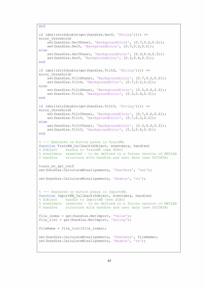
65

end if (abs((str2double(get(handles.DecY, 'String')))) >= error_threshold) set(handles.DecYPanel, 'BackgroundColor', [0.7,0.2,0.2]); set(handles.DecY, 'BackgroundColor', [0.7,0.2,0.2]); else set(handles.DecYPanel, 'BackgroundColor', [0.3,0.6,0.3]); set(handles.DecY, 'BackgroundColor', [0.3,0.6,0.3]); end if (abs((str2double(get(handles.TiltX, 'String')))) >= error_threshold) set(handles.TiltXPanel, 'BackgroundColor', [0.7,0.2,0.2]); set(handles.TiltX, 'BackgroundColor', [0.7,0.2,0.2]); else set(handles.TiltXPanel, 'BackgroundColor', [0.3,0.6,0.3]); set(handles.TiltX, 'BackgroundColor', [0.3,0.6,0.3]); end if (abs((str2double(get(handles.TiltY, 'String')))) >= error_threshold) set(handles.TiltYPanel, 'BackgroundColor', [0.7,0.2,0.2]); set(handles.TiltY, 'BackgroundColor', [0.7,0.2,0.2]); else set(handles.TiltYPanel, 'BackgroundColor', [0.3,0.6,0.3]); set(handles.TiltY, 'BackgroundColor', [0.3,0.6,0.3]); end % --- Executes on button press in TrainNN. function TrainNN_Callback(hObject, eventdata, handles) % hObject handle to TrainNN (see GCBO) % eventdata reserved - to be defined in a future version of MATLAB % handles structure with handles and user data (see GUIDATA) train_nn_zpl_out2 set(handles.CalculateMisalignments, 'UserData', 'net'); set(handles.CalculateMisalignments, 'Enable', 'on'); % --- Executes on button press in ImportNN. function ImportNN_Callback(hObject, eventdata, handles) % hObject handle to ImportNN (see GCBO) % eventdata reserved - to be defined in a future version of MATLAB % handles structure with handles and user data (see GUIDATA) file_index = get(handles.NetImport, 'Value'); file_list = get(handles.NetImport, 'String'); fileName = file_list{file_index}; set(handles.CalculateMisalignments, 'UserData', fileName); set(handles.CalculateMisalignments, 'Enable', 'on');

66

% --- Executes on button press in Built_inNN. function Built_inNN_Callback(hObject, eventdata, handles) % hObject handle to Built_inNN (see GCBO) % eventdata reserved - to be defined in a future version of MATLAB % handles structure with handles and user data (see GUIDATA) set(handles.CalculateMisalignments, 'UserData', 'net'); set(handles.CalculateMisalignments, 'Enable', 'on'); % --- If Enable == 'on', executes on mouse press in 5 pixel border. % --- Otherwise, executes on mouse press in 5 pixel border or over TextFileSelect. function TextFileSelect_ButtonDownFcn(hObject, eventdata, handles) % hObject handle to TextFileSelect (see GCBO) % eventdata reserved - to be defined in a future version of MATLAB % handles structure with handles and user data (see GUIDATA) % --- Executes on selection change in TextFileSelect. function listbox1_Callback(hObject, eventdata, handles) % hObject handle to TextFileSelect (see GCBO) % eventdata reserved - to be defined in a future version of MATLAB % handles structure with handles and user data (see GUIDATA) % Hints: contents = cellstr(get(hObject,'String')) returns TextFileSelect contents as cell array % contents{get(hObject,'Value')} returns selected item from TextFileSelect % --- Executes during object creation, after setting all properties. function listbox1_CreateFcn(hObject, eventdata, handles) % hObject handle to TextFileSelect (see GCBO) % eventdata reserved - to be defined in a future version of MATLAB % handles empty - handles not created until after all CreateFcns called % Hint: listbox controls usually have a white background on Windows. % See ISPC and COMPUTER. if ispc && isequal(get(hObject,'BackgroundColor'), get(0,'defaultUicontrolBackgroundColor')) set(hObject,'BackgroundColor','white'); end function edit1_Callback(hObject, eventdata, handles) % hObject handle to edit1 (see GCBO) % eventdata reserved - to be defined in a future version of MATLAB % handles structure with handles and user data (see GUIDATA) % Hints: get(hObject,'String') returns contents of edit1 as text % str2double(get(hObject,'String')) returns contents of edit1 as a double

67

% --- Executes during object creation, after setting all properties. function edit1_CreateFcn(hObject, eventdata, handles) % hObject handle to edit1 (see GCBO) % eventdata reserved - to be defined in a future version of MATLAB % handles empty - handles not created until after all CreateFcns called % Hint: edit controls usually have a white background on Windows. % See ISPC and COMPUTER. if ispc && isequal(get(hObject,'BackgroundColor'), get(0,'defaultUicontrolBackgroundColor')) set(hObject,'BackgroundColor','white'); end function edit2_Callback(hObject, eventdata, handles) % hObject handle to edit2 (see GCBO) % eventdata reserved - to be defined in a future version of MATLAB % handles structure with handles and user data (see GUIDATA) % Hints: get(hObject,'String') returns contents of edit2 as text % str2double(get(hObject,'String')) returns contents of edit2 as a double % --- Executes during object creation, after setting all properties. function edit2_CreateFcn(hObject, eventdata, handles) % hObject handle to edit2 (see GCBO) % eventdata reserved - to be defined in a future version of MATLAB % handles empty - handles not created until after all CreateFcns called % Hint: edit controls usually have a white background on Windows. % See ISPC and COMPUTER. if ispc && isequal(get(hObject,'BackgroundColor'), get(0,'defaultUicontrolBackgroundColor')) set(hObject,'BackgroundColor','white'); end function edit3_Callback(hObject, eventdata, handles) % hObject handle to edit3 (see GCBO) % eventdata reserved - to be defined in a future version of MATLAB % handles structure with handles and user data (see GUIDATA) % Hints: get(hObject,'String') returns contents of edit3 as text % str2double(get(hObject,'String')) returns contents of edit3 as a double % --- Executes during object creation, after setting all properties. function edit3_CreateFcn(hObject, eventdata, handles)

68

% hObject handle to edit3 (see GCBO) % eventdata reserved - to be defined in a future version of MATLAB % handles empty - handles not created until after all CreateFcns called % Hint: edit controls usually have a white background on Windows. % See ISPC and COMPUTER. if ispc && isequal(get(hObject,'BackgroundColor'), get(0,'defaultUicontrolBackgroundColor')) set(hObject,'BackgroundColor','white'); end function edit4_Callback(hObject, eventdata, handles) % hObject handle to edit4 (see GCBO) % eventdata reserved - to be defined in a future version of MATLAB % handles structure with handles and user data (see GUIDATA) % Hints: get(hObject,'String') returns contents of edit4 as text % str2double(get(hObject,'String')) returns contents of edit4 as a double % --- Executes during object creation, after setting all properties. function edit4_CreateFcn(hObject, eventdata, handles) % hObject handle to edit4 (see GCBO) % eventdata reserved - to be defined in a future version of MATLAB % handles empty - handles not created until after all CreateFcns called % Hint: edit controls usually have a white background on Windows. % See ISPC and COMPUTER. if ispc && isequal(get(hObject,'BackgroundColor'), get(0,'defaultUicontrolBackgroundColor')) set(hObject,'BackgroundColor','white'); end function edit5_Callback(hObject, eventdata, handles) % hObject handle to edit5 (see GCBO) % eventdata reserved - to be defined in a future version of MATLAB % handles structure with handles and user data (see GUIDATA) % Hints: get(hObject,'String') returns contents of edit5 as text % str2double(get(hObject,'String')) returns contents of edit5 as a double % --- Executes during object creation, after setting all properties. function edit5_CreateFcn(hObject, eventdata, handles) % hObject handle to edit5 (see GCBO) % eventdata reserved - to be defined in a future version of MATLAB % handles empty - handles not created until after all CreateFcns called

69

% Hint: edit controls usually have a white background on Windows. % See ISPC and COMPUTER. if ispc && isequal(get(hObject,'BackgroundColor'), get(0,'defaultUicontrolBackgroundColor')) set(hObject,'BackgroundColor','white'); end function edit6_Callback(hObject, eventdata, handles) % hObject handle to edit6 (see GCBO) % eventdata reserved - to be defined in a future version of MATLAB % handles structure with handles and user data (see GUIDATA) % Hints: get(hObject,'String') returns contents of edit6 as text % str2double(get(hObject,'String')) returns contents of edit6 as a double % --- Executes during object creation, after setting all properties. function edit6_CreateFcn(hObject, eventdata, handles) % hObject handle to edit6 (see GCBO) % eventdata reserved - to be defined in a future version of MATLAB % handles empty - handles not created until after all CreateFcns called % Hint: edit controls usually have a white background on Windows. % See ISPC and COMPUTER. if ispc && isequal(get(hObject,'BackgroundColor'), get(0,'defaultUicontrolBackgroundColor')) set(hObject,'BackgroundColor','white'); end function edit7_Callback(hObject, eventdata, handles) % hObject handle to edit7 (see GCBO) % eventdata reserved - to be defined in a future version of MATLAB % handles structure with handles and user data (see GUIDATA) % Hints: get(hObject,'String') returns contents of edit7 as text % str2double(get(hObject,'String')) returns contents of edit7 as a double % --- Executes during object creation, after setting all properties. function edit7_CreateFcn(hObject, eventdata, handles) % hObject handle to edit7 (see GCBO) % eventdata reserved - to be defined in a future version of MATLAB % handles empty - handles not created until after all CreateFcns called % Hint: edit controls usually have a white background on Windows. % See ISPC and COMPUTER. if ispc && isequal(get(hObject,'BackgroundColor'),

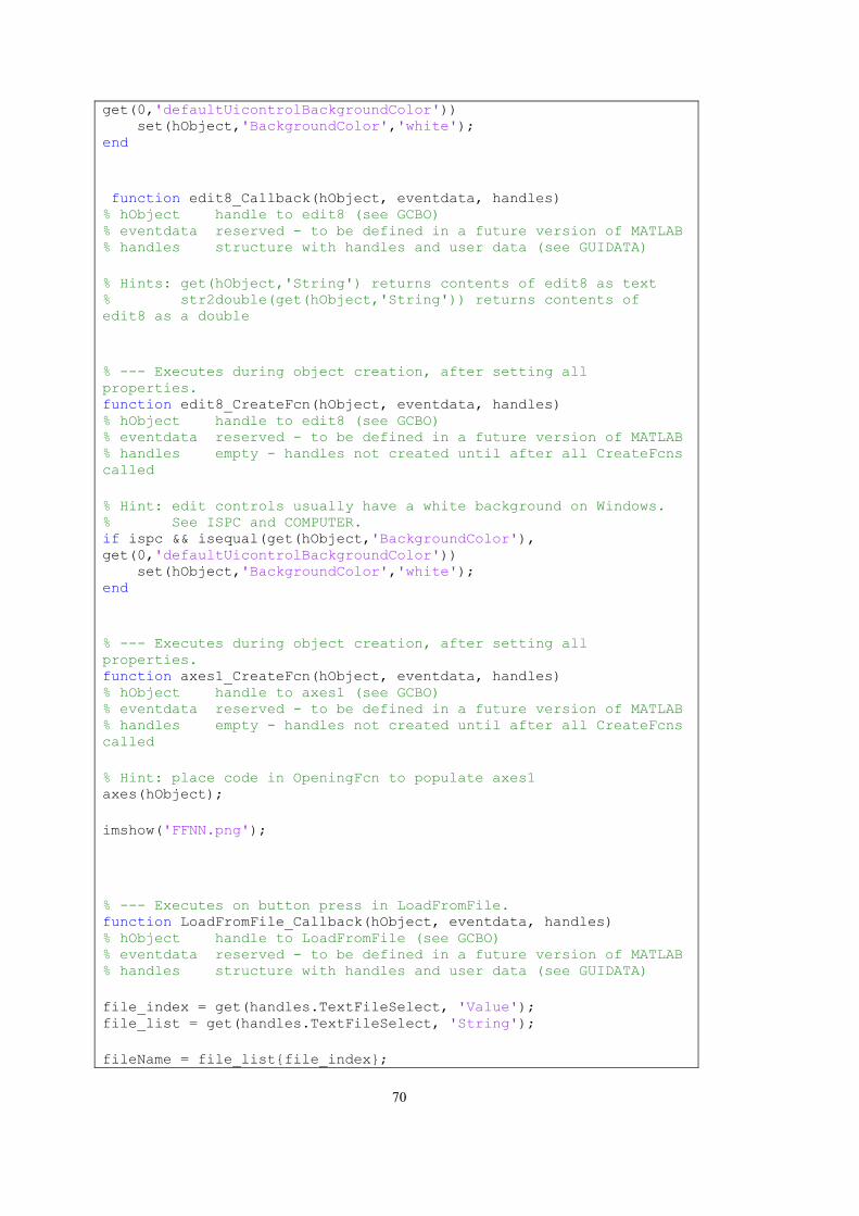
70

get(0,'defaultUicontrolBackgroundColor')) set(hObject,'BackgroundColor','white'); end function edit8_Callback(hObject, eventdata, handles) % hObject handle to edit8 (see GCBO) % eventdata reserved - to be defined in a future version of MATLAB % handles structure with handles and user data (see GUIDATA) % Hints: get(hObject,'String') returns contents of edit8 as text % str2double(get(hObject,'String')) returns contents of edit8 as a double % --- Executes during object creation, after setting all properties. function edit8_CreateFcn(hObject, eventdata, handles) % hObject handle to edit8 (see GCBO) % eventdata reserved - to be defined in a future version of MATLAB % handles empty - handles not created until after all CreateFcns called % Hint: edit controls usually have a white background on Windows. % See ISPC and COMPUTER. if ispc && isequal(get(hObject,'BackgroundColor'), get(0,'defaultUicontrolBackgroundColor')) set(hObject,'BackgroundColor','white'); end % --- Executes during object creation, after setting all properties. function axes1_CreateFcn(hObject, eventdata, handles) % hObject handle to axes1 (see GCBO) % eventdata reserved - to be defined in a future version of MATLAB % handles empty - handles not created until after all CreateFcns called % Hint: place code in OpeningFcn to populate axes1 axes(hObject); imshow('FFNN.png'); % --- Executes on button press in LoadFromFile. function LoadFromFile_Callback(hObject, eventdata, handles) % hObject handle to LoadFromFile (see GCBO) % eventdata reserved - to be defined in a future version of MATLAB % handles structure with handles and user data (see GUIDATA) file_index = get(handles.TextFileSelect, 'Value'); file_list = get(handles.TextFileSelect, 'String'); fileName = file_list{file_index};

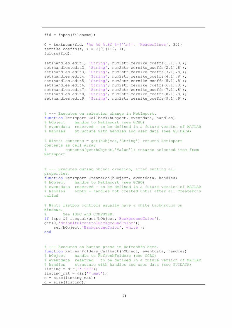
71

fid = fopen(fileName); C = textscan(fid, '%s %d %.8f %*[^\n]', 'HeaderLines', 30); zernike_coeffs(:,1) = C{3}(1:9, 1); fclose(fid); set(handles.edit1, 'String', num2str(zernike_coeffs(1,1),8)); set(handles.edit2, 'String', num2str(zernike_coeffs(2,1),8)); set(handles.edit3, 'String', num2str(zernike_coeffs(3,1),8)); set(handles.edit4, 'String', num2str(zernike_coeffs(4,1),8)); set(handles.edit5, 'String', num2str(zernike_coeffs(5,1),8)); set(handles.edit6, 'String', num2str(zernike_coeffs(6,1),8)); set(handles.edit7, 'String', num2str(zernike_coeffs(7,1),8)); set(handles.edit8, 'String', num2str(zernike_coeffs(8,1),8)); set(handles.edit9, 'String', num2str(zernike_coeffs(9,1),9)); % --- Executes on selection change in NetImport. function NetImport_Callback(hObject, eventdata, handles) % hObject handle to NetImport (see GCBO) % eventdata reserved - to be defined in a future version of MATLAB % handles structure with handles and user data (see GUIDATA) % Hints: contents = get(hObject,'String') returns NetImport contents as cell array % contents{get(hObject,'Value')} returns selected item from NetImport % --- Executes during object creation, after setting all properties. function NetImport_CreateFcn(hObject, eventdata, handles) % hObject handle to NetImport (see GCBO) % eventdata reserved - to be defined in a future version of MATLAB % handles empty - handles not created until after all CreateFcns called % Hint: listbox controls usually have a white background on Windows. % See ISPC and COMPUTER. if ispc && isequal(get(hObject,'BackgroundColor'), get(0,'defaultUicontrolBackgroundColor')) set(hObject,'BackgroundColor','white'); end % --- Executes on button press in RefreshFolders. function RefreshFolders_Callback(hObject, eventdata, handles) % hObject handle to RefreshFolders (see GCBO) % eventdata reserved - to be defined in a future version of MATLAB % handles structure with handles and user data (see GUIDATA) listing = dir('*.TXT'); listing_mat = dir('*.mat'); e = size(listing_mat); d = size(listing);

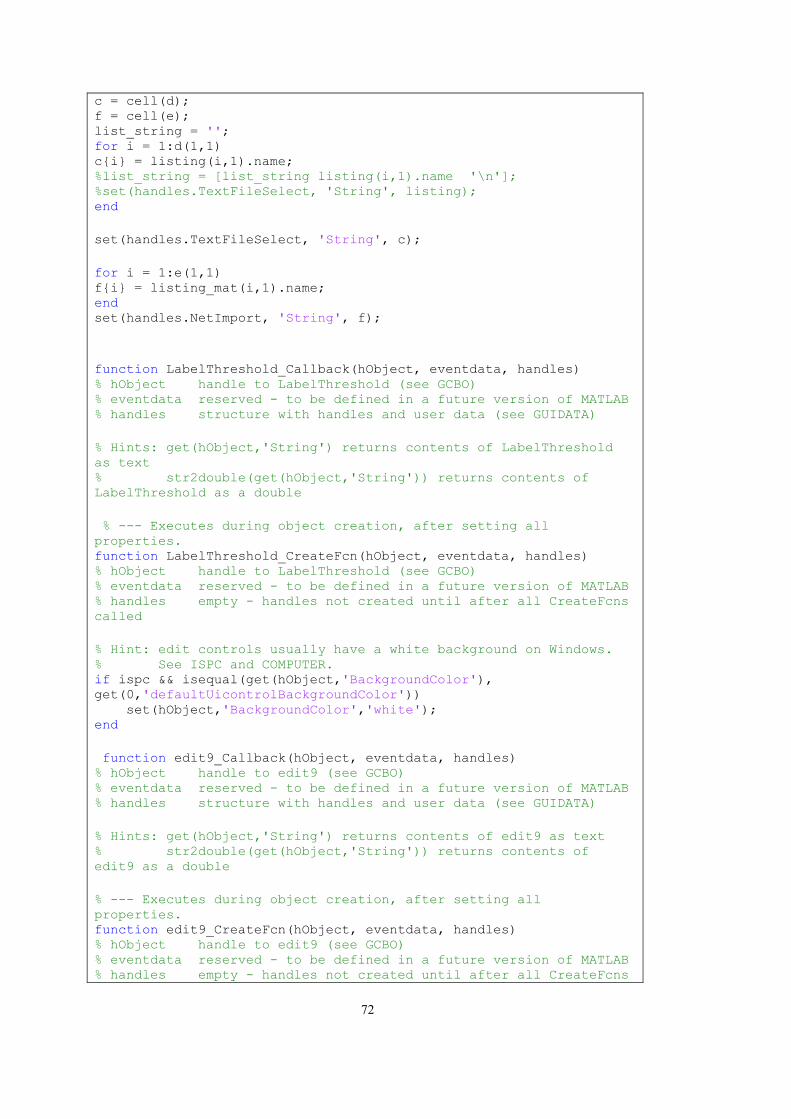
72

c = cell(d); f = cell(e); list_string = ''; for i = 1:d(1,1) c{i} = listing(i,1).name; %list_string = [list_string listing(i,1).name '\n']; %set(handles.TextFileSelect, 'String', listing); end set(handles.TextFileSelect, 'String', c); for i = 1:e(1,1) f{i} = listing_mat(i,1).name; end set(handles.NetImport, 'String', f); function LabelThreshold_Callback(hObject, eventdata, handles) % hObject handle to LabelThreshold (see GCBO) % eventdata reserved - to be defined in a future version of MATLAB % handles structure with handles and user data (see GUIDATA) % Hints: get(hObject,'String') returns contents of LabelThreshold as text % str2double(get(hObject,'String')) returns contents of LabelThreshold as a double % --- Executes during object creation, after setting all properties. function LabelThreshold_CreateFcn(hObject, eventdata, handles) % hObject handle to LabelThreshold (see GCBO) % eventdata reserved - to be defined in a future version of MATLAB % handles empty - handles not created until after all CreateFcns called % Hint: edit controls usually have a white background on Windows. % See ISPC and COMPUTER. if ispc && isequal(get(hObject,'BackgroundColor'), get(0,'defaultUicontrolBackgroundColor')) set(hObject,'BackgroundColor','white'); end function edit9_Callback(hObject, eventdata, handles) % hObject handle to edit9 (see GCBO) % eventdata reserved - to be defined in a future version of MATLAB % handles structure with handles and user data (see GUIDATA) % Hints: get(hObject,'String') returns contents of edit9 as text % str2double(get(hObject,'String')) returns contents of edit9 as a double % --- Executes during object creation, after setting all properties. function edit9_CreateFcn(hObject, eventdata, handles) % hObject handle to edit9 (see GCBO) % eventdata reserved - to be defined in a future version of MATLAB % handles empty - handles not created until after all CreateFcns

73

called % Hint: edit controls usually have a white background on Windows. % See ISPC and COMPUTER. if ispc && isequal(get(hObject,'BackgroundColor'), get(0,'defaultUicontrolBackgroundColor')) set(hObject,'BackgroundColor','white'); end

74

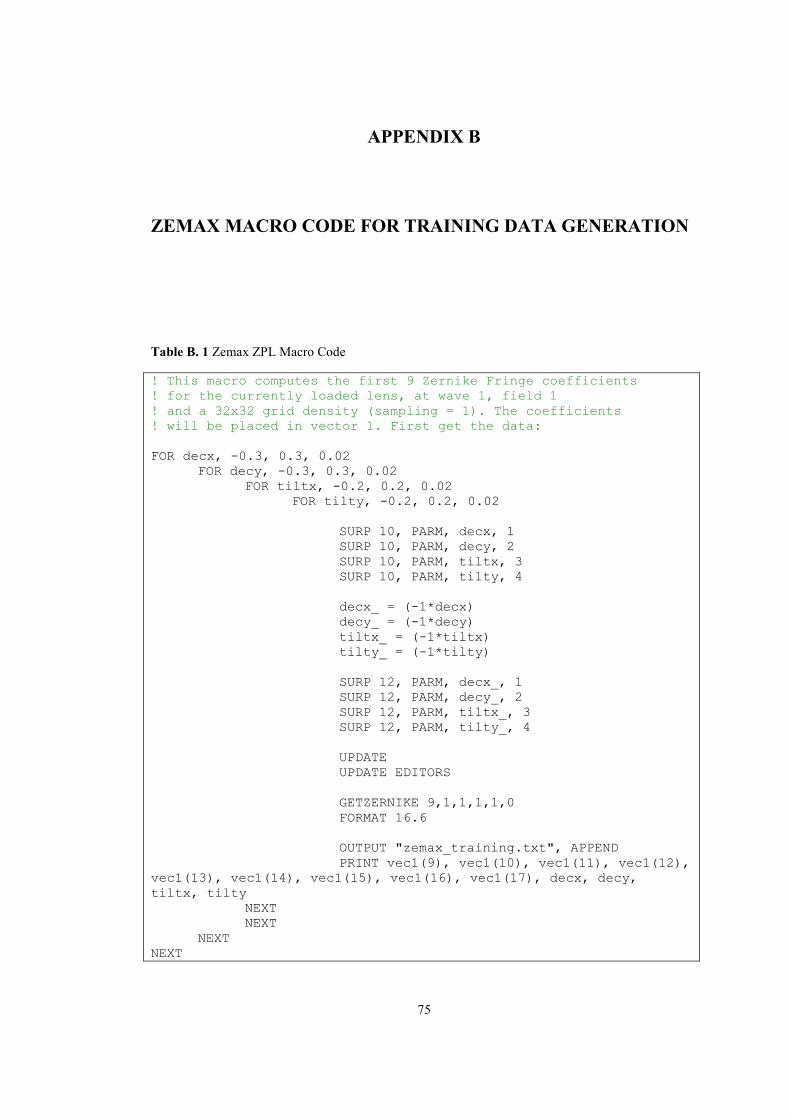
75

.

APPENDIX B

ZEMAX MACRO CODE FOR TRAINING DATA GENERATION

Table B. 1 Zemax ZPL Macro Code

! This macro computes the first 9 Zernike Fringe coefficients ! for the currently loaded lens, at wave 1, field 1 ! and a 32x32 grid density (sampling = 1). The coefficients ! will be placed in vector 1. First get the data: FOR decx, -0.3, 0.3, 0.02 FOR decy, -0.3, 0.3, 0.02 FOR tiltx, -0.2, 0.2, 0.02 FOR tilty, -0.2, 0.2, 0.02 SURP 10, PARM, decx, 1 SURP 10, PARM, decy, 2 SURP 10, PARM, tiltx, 3 SURP 10, PARM, tilty, 4 decx_ = (-1*decx) decy_ = (-1*decy) tiltx_ = (-1*tiltx) tilty_ = (-1*tilty) SURP 12, PARM, decx_, 1 SURP 12, PARM, decy_, 2 SURP 12, PARM, tiltx_, 3 SURP 12, PARM, tilty_, 4 UPDATE UPDATE EDITORS GETZERNIKE 9,1,1,1,1,0 FORMAT 16.6 OUTPUT "zemax_training.txt", APPEND PRINT vec1(9), vec1(10), vec1(11), vec1(12), vec1(13), vec1(14), vec1(15), vec1(16), vec1(17), decx, decy, tiltx, tilty NEXT NEXT NEXT NEXT

.

76

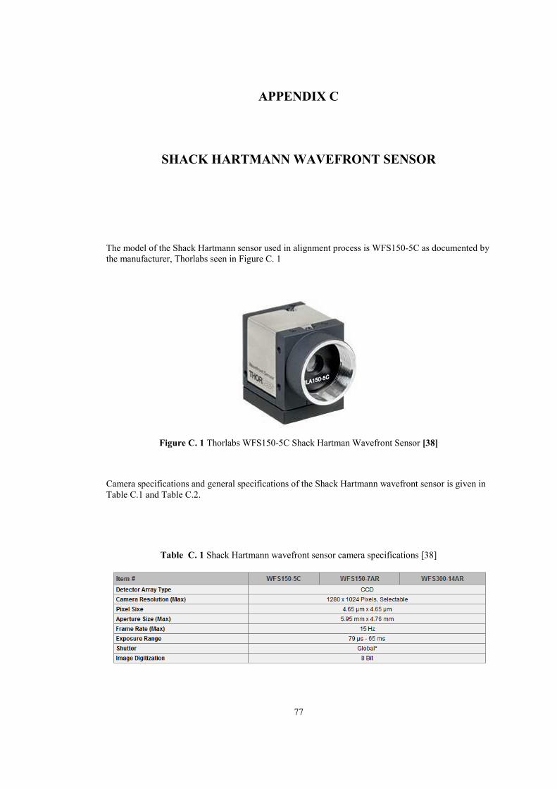
77

.

APPENDIX C

SHACK HARTMANN WAVEFRONT SENSOR

The model of the Shack Hartmann sensor used in alignment process is WFS150-5C as documented by the manufacturer, Thorlabs seen in Figure C. 1

Figure C. 1 Thorlabs WFS150-5C Shack Hartman Wavefront Sensor [38]

Camera specifications and general specifications of the Shack Hartmann wavefront sensor is given in

Table C.1 and Table C.2.

Table C. 1 Shack Hartmann wavefront sensor camera specifications [38]

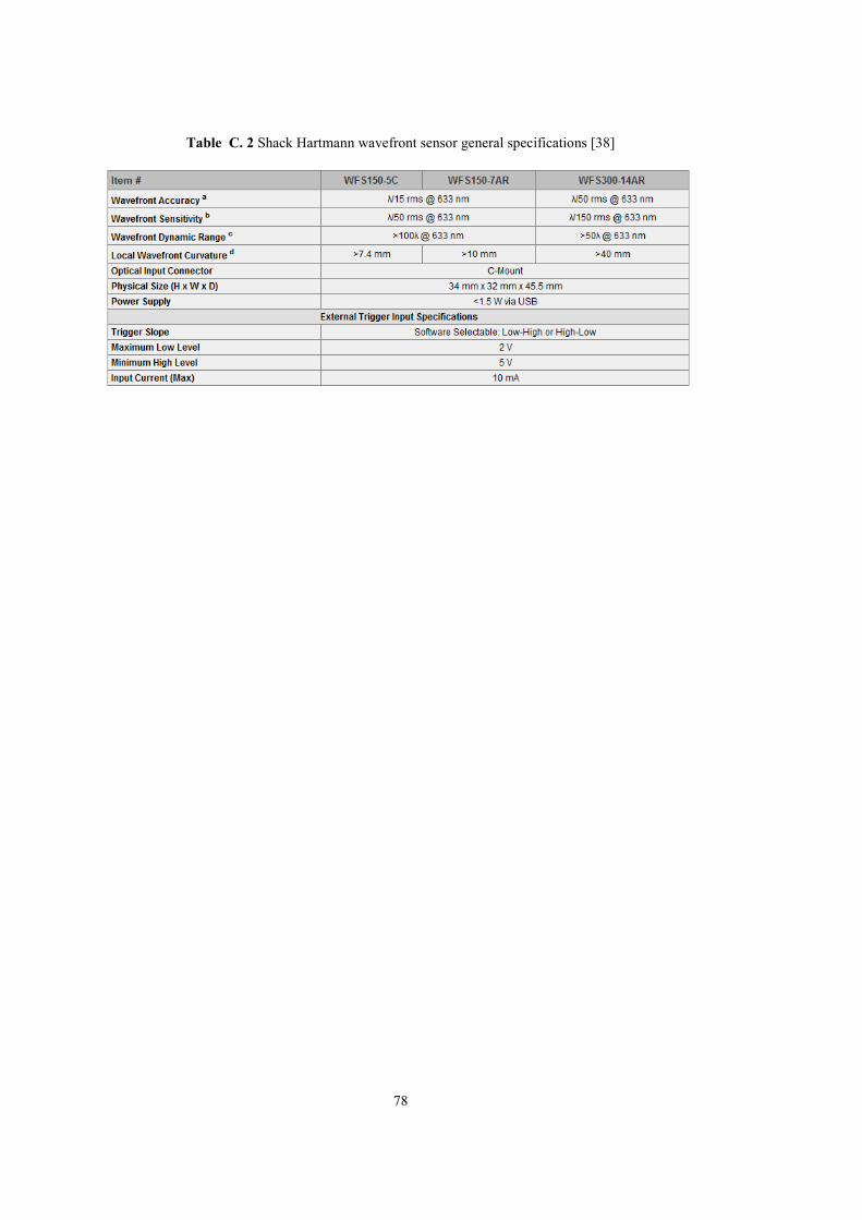
78

Table C. 2 Shack Hartmann wavefront sensor general specifications [38]

79

...

APPENDIX D

CALIBRATION AND TEST PROCEDURE OF THE VISOR

ALIGNMENT TEST SETUP

Table D. 1 Equipment List

TEST EQUIPMENT LIST

DESCRIPTION SUPPLIER MODEL/ VERSION

Shack Hartmann Wavefront Sensor Thorlabs WFS-150-5C

Reference Laser Thorlabs HGR20

Beam Expander Thorlabs BE10M

Beam Splitters Thorlabs CM1-BS013

2 inch Flat Mirrors Thorlabs PF20-03-P01-10

2inch Mirror Mounts Thorlabs KM200

Pinhole Diaphragms Newport ID-1.0

Expander Objective Aselsan -

Rotation Stage Newport M-UTR46A

Tilt Stage Newport M-TTN80

Linear Stages Newport M-460A

1. TEST CONDITION REQUIREMENTS

Ambient Requirements

Temperature: Room ambient Relative Humidity: Room ambient

2. CALIBRATION PROCEDURE OF THE OPTICAL TEST SETUP

Note: Verify the calibration of the setup every 6 months.

2.1 Verify that all the optical elements are configured as shown in Figure 28 and Figure 29.

2.2 Replace the objectives and visor parts with flat mirror. 2.3 Use the autocollimator to configure the mirror as parallel to the optical table plane. 2.4 Switch on the reference laser. 2.5 As the first step, verify that the reference laser hits the centers of the 2 diaphrams located opposite to the beam splitters. 2.6 If laser does not hit the centers of the diaphragms, align the optical path by using the micrometer probes of the flat mirrors.

80

2.7 Remove the flat mirror and place the objective back to its holder. 2.8 Mount the pin holes of the objectives to make the laser beams hit the centers of the objectives as shown in Figure 45. 2.9 Place SHWS after the objective and verify that the measured Zernike coefficient values are less than or equal to the values given in Table 2. If the values are greater than these values, adjust the linear probes under the objectives until the values are less than or equal to the values given in Table 2. 2.10 Calibration procedure is concluded.

3. TEST PROCEDURE OF THE OPTICAL TEST SETUP

3.1 Switch on the reference laser. 3.2 Switch on the air supply of the vacuum holder and put the visor on the holder. 3.3 Adjust the visor holder until the back reflection of the laser falls on SHWS. 3.4 In the sensor software window, move the laser spot to the center of the reticle. 3.5 Insert the first 9 Zernike coefficients into the fields on the Alignment Correction Software interface. 3.6 Apply the decenters along X, Y directions and tilts around X, Y axes given by the Alignment Correction Software on the adjustment mechanisms of the visor holder. 3.7 After the application of Alignment Correction Method results on the visor holder, repeat the

procedure until all Zernike coefficients read from SHWS fall within the range of [-1, 1].