//^(fr/7

f^ffff ^fyi Bfffft ^%^^i^Mni^ia

For ittteaHWAc •aoi l ii

Bkiiii:;i.

PREFACE

This xs one of a series of methodology transfer papers developed by the Institute for Program Evaluation. The purpoae of a methodology transfer paper is to provide GAO evaluators with a clear and comprehensive background of the basic concepts of an evaluation methodology. Additionally, general and spe­cific applications and procedures for using the evaluation methodology are provided.

The paper defines and describes an evaluation method-causal analysis. Causal analysis is not a panacea for evalua­ting programs. Like all evaluation techniques, it has advan­tages and limitatiena. Causal analysis is offered, however, as one way to improve the quality of some GAO evaluations.

TO THE READER

This paper is designed to be self-instructional. Through reading it, you should be able to gain (1) an understanding of the basic concepts and techniques for using cauaal analysis and (2) the ability to recognize appropriate circumstances in a job for using l^ese techniques. The body of the paper contains, for the mosl part, non-technical information. Appendix I ia a gloa-smry of technical terms. Appendix II and appendix III should be vaiuai!>le to anyone %fho plana to make or wishes to understand the statistical calculations used in causal analysis. Appendix II provides S!tef by step instructions for using the statistical technique of path analysis. Appendix III presents an example of applying causal analysis to the evaluation of prison parole out-

Portunately, an evaluator has several resources available at GAO to help with any statistical analysis. The Specialized Skills/Technical Aaaistance Group in the Institute for Program Bvaluation can provide direct support to an evaluator. Addi­tionally, the evaluator has access, through any GAO computer terminal, to statistical paclcagea—such as SPSS (Statistical Package for the Social Sciences)—that perform the statisti­cal conqputations.

We would appreciate comments on the job-related usefulness of this paper. A brief questionnaire is provided for this pur­pose on a tear-out sheet on the last page.

i

I OVERVIEW

» Causal analysis helps an evaluator identify what affects program results and to %^at extent. Causal analysis helps answer questions such as: What combination of program pro-

I cedures, components, resources, and constraints causes a par-I ticular result? To what extent do economic, social, and politi-I cal factors affect a program?

Causal analysis ia a t«ro-phase process. The first phaae— causal modeling—can be used to deacribe assumed cause and effect relationships between program outcome(s) and certain key factors and activities from within and outside the program. The second phaae—path analysis—ia us4kl to analyze statistically the assumed causal relations. Thia second phaae may be infeasi-ble because of data or other restrictions. Nevertheless, causal modeling alone enables evaluators to develop a systeauitie under­standing of assumed cause/effect relationships.

This paper deserilMS <uid illustrates applying causal analy­sis in program evaluation. It presents a framework for modeling eaiase and effect relationships, inatructions for teating a model*a adequacy and for estiauiting the relative atrength of direct and indirect influences, and examples of using the tech­nique.

Chapter 1 discusses the concept of causality and its rele­vance to program evaluators. It spseifies three conditions that should be analysed before inferring that a causal relationship exists between two piM

Chapter 2 presents an approscAi for constructing causal for program evaluation. This approach requires evalua­

tors to:

—establish the evaluation's scope and focus by specifying a finite set of variables,

—amdce assumptions about the selected variables' causal intsrrelatsdness and about the effects of known variables that are oadtted, and

'—test the model's adequacy by dstsrodning whether it is consistent with data.

Path analyais, describsd in chapter 3, is a atatistical technique that can be uaed to test a causal model's adequacy based on predetermined criteria. Thia technique requires con­structing a "path diagram" of the major variables and their relationships, calculating the magnitude of the assumsd causal associations, analysing and reviaing the assumptions, and inter­preting the final path diagram. This chapter defines path analyaia and discusses data requirementa and potential applica-tiona in program evaluation.

Chapter 4 diacusses potential applications of causal analy­sis in program evaluation. It examinee three general evaluation situations in which the technique can be applied*

—to find out if an observed effect %ms really due j: to a program or activity,

I —to identify a program*a effacta, or

t I 1 1

-J

—to underatand %#hy a program had a consequence other than %ihat «#as expected.

Examples and a few variations of these situations are presented to show how causal models could be specified and how path analysis may be used. Finally, soms of the limitationa of cauaal analysis are discussed.

Many people contributed to this document via the review process. In particular, we benefited from peer reviews by four­teen staff from e Inatitute for Program Evaluation and from

: outside reviews by Hubert Blalock (University of Washington), j Saul Gass (University of Maryland), Larry Gordon (University of

Maryland), and Michael Seriven (University of San Francisco). We gratefully aelcnowledge their assistance.

The document %ms developed in the Methodology Development and Data Assistance Group, under Keith R. Marvin, Associate Dlrsctor; by Bruce W. Thompson, Group Oirsctor; and by Larry

i Hedges, Tesm Leader, assisted by Teresa Spisidt, Sandra Thibault, 1 mad\ Ptt^iek Dynes. The project also involved the efforts of

ro of our teehnical assistance group: Wayne Dow and Steve

Eleanor Chelimsky J Director, Institute for Program Bvaluation

ill

1-

c o n t e n t

PREFACE

CHAPTER

1

tmpmsDmn

I

II

INTRODUCTION What ia causality? Causal thinking and program evaluation

Bibliography

CONSTRUCTING CAUSAL MODELS FOR PROGRAM EVALUATION

Selecting variables to study Establishing the evalua­

t ion ' s focus Speei^ing the isgiortant

Making assumptions about causal relationships

Testing e model's adequacy

Bibliography

PATH ANALYSIS What is path analysis? Data collection Applications in program evaluation Program oosQiarisons Analysing multiple results Reciprocal eaos«is and effects

Joint causes Idwati^ing underlying concepts

Summsry Bibliography

WHEN IS CAUSAL ANALYSIS APPRO-

Appropriate cases Limitationa

Glossary of teehnical terras

Gheeklist of steps in path analysis

iv

Page

1

1 1

3 5

6 6

12 15 15 17

16 18

21 21 22

29 25

25 27 28

30 30 33 34

35

37

ijitij

Page

III Cauaal analysis of parole outcomes 49

FIGURE

2.1 Baaic mechanisms of a hams visit program 7

2.2 Suchman's model of intervening variola analysis 8

2.3 The genorsl systow model 10

2.4 Components of a tj^ical program 10

2.5 Causal relationships within the context

of a program 13

2.6 Model of a hypothetical prison parole process 14

3.1 Bvmlintlon of teaeher training 19

3.2 Pat;h dla^aii relating edueatienal amplrations . ,to' .||ptittK9e., soeioeeonomic statoS:, and

I, by smx 22 3w3 The rsclprocs*. effeets of oecupmtiemml

eonditiotts snd intsllsetnml flexibility 24

3.4 9mit% diagram using factor anmlysis 26

XZ.1 prellsilnary pmUi diagram 38 Xi..2 Statistical assomptioms and implieatieos for

datm analysis 41

is. 3 H f rescsdamtic residaals 42

11.4 ealeulatlng direct and indirect paths 44

XI1.1 Gsmmral causal aodel e^lainlng parole ontceaw 50 I-

1X1.2 TlM first 10 factors and salient variables 52

XX1.3 Znitlal causal model for determining parole

outeoaias 54

I XIX.4 Prsllmlnary path diagram 55

XXX..5 Example of oomputer output 57

IXI.€ Preliminary model with path values 58 III.7 Rmvlsed aedei for determining parole outcomes

using :pa<th analysis 60

XXI.6 Direct snd indirect paths 61

14 iiSijaiSasliikiJ jv-c •

ii

CHAPTER 1

INTRODUCTION

This paper is for anyone %iho atudies causs and effect relationa. It describes and illustrates an approach for explain­ing any phenoawnon (effect) as the result of another phenomenon (cause). The paper containas

overview of causal analysis in evaluating prograflM,

approach for modeling presumed cause and effect relations,

— a procedure, path analysis, for testing thm adequacy of the model, and

—msamplmm of applying causal modeling wad path

maa xs mammMTXi k GmiMelity allies Whenever one phemommnon appears to imply

the oeempreniOS of anoUisr. Seriven defines causation as ths rmim^iom be wmmn oosquitos sad mosquito oites. The eomcept is

lily wHlmrstood, although it has never been satisfactorily

authors 2 / have specified conditions that should be to infer m existence of a causal relationship between two

or irairiadsles. Generally, a causal relationship can be laaittErsd by analysing.:

1. how the phenomena are ordered in tioM,

2. %Aether they are relateu or associated, and

3. lAmther the relationship is due to chance or other factors.

In the first condition, one phenomenc«n may precede the oi^mr or the two may occur simultaneously. For examplm, striking a bell, X, is followed by ringing of the bell, Y. FUirthermore, if X causes Y, it does not follow Uiat a change In y produces a change in X. Thua, a change in rainfall may prodnee a change in %dieat yields, but a change in «diea<t yields dloes not produce a change in rainfall. 3/

\ivmn L8J, p* 19*

2/See« for example, Ackoff [13, P* 16 and Asher [23, p. 11.

3/Blaloek C3i^ p. 10.

Additionally, t%»o phenemmna may occur simultaneously and still be causally related. 1 / For example, one could study ths effect that a studsnt's intelligence quotient (IQ) has on col-legs grade point average (OPA).

Tims sequence can indicste s caossl rslationship among dis­crete phenomsns, att<;h as strilcing a bell being followed lay ring­ing of the bell. Bowmvmr, many phenomena sueh as population growth and attitude changms vary eontinuoualy. A causal rela­tionship among coatinuoua phenosmna may be inferred by analysing «dieti»er they are related or associated.

For the aeeond oondltlon, tiiersiers, an svaluator looks for a concomitant veriation or covariation between X and Y: Whether chwiges in one phsnommnon are accompanied by cAianget. in the other. For examplmt correlsition anmlysis mig^t show for SCSM general poptt-lat,loa thm^ tiie hl ier a stndmnt's XQ« the higher the GPA, snd , convmrsmly, ths lowmr \3bm X0« tfte lower the OPA. In this •sample* 10 mmy be eonsldmrsd a "wsak" oaoss sines anuiy o^sr vmr^l^les affect GPA. soms of those variables may even act to Obseurm I3im association betwmsn XQ and OPA.

FlnM.ly, t3»e third oondltloa requires an evaluator to ilsiiiistrmtm t3wt ths relatttonahlp of ths phsnoswina 11 not due to cllmnee. This eaewpliflee I9is wmll- known slogan that "eorrsla-tifOQ is no iproof of esmsmtien. ** Thus, "spurious correlation*— a reimtlonmhip Jbetmmmn two variable Umit are net oausally iater-rmietmd, slliHMij^ thmy may at first sppmsr to bo->->;mist be com-sld^emdw

AiCiko£f 2/ gimes a good illusttrmttioa of spurious oorrslation. Ho elitms taie -dlscovmry that: pmopls who livs In nml^^dmrhoods having hmmvy meot-fall ars more llkmly to contrset twbsrealeols l imn peeple Who live in nmlg itoorhoeds hmvlng loss soot-fall. Basmd on this oorxwlmtlem, oms rsmmsrchsr oomelndmd tiiat soot-abrnm^^p^^b ^mm^p^^mmsm^v^^pem epmsmi^^^p^v'^vma m^i^^^p wb v m evemai^^^^^^^eme^^^^mm^^v ^b'^^^^v^^^^B^b ^^ssi^ S^H^^^^^S'^F'^VJ^P IS

showmd tJist dietioif defieismeims prodmcc tobsrenlosis. dietary deflelenelms are llkmly to oeeur most frmqumntly low-lnooaw groups, trnw tnrems groups are liksly to livm In low^rmt dletrlets. Districts hsvm low rmnt, amomg otiimr <Silmgs, bmemums of heavy soot-fall. Thus, soot-fall and tutosreulosis are sceidmntally, not eaosmlly

eausality has be«i dsf Inmd in many ways and has iMsn ths sWbjeet of considmrsble philomepldical dlaeusslon. SOBM philc phmrs have oibjsetmd to causal thinking because* "(1) eausality can never be verified empirically sad (2) the notion of oause and effect is far too simple to describe reality, with causal

1/Bleks rs], pp. 21-25.

2/AdBof£ £13» P- 18.

- ' " ' •

laws being much more a property of the observer than of the real %#orld itaelf." 1/ Nevertheless, others believe the mere question­ing of "why" an event occurred implies causality. In addition, as Cooley points out, "most of what is known about people and the universe has not been based on experimentation, but on observa­tion." \ l Cooley*s philosophy is that to understand a process in a way tKat will allow improvements, attention muat be given to "developing methods for conducting explanatory observational stud­ies." Causation in this sense is an iagiortant topic to evaluator a.

CAUSAL THINKING AND PROGRAM EVALUATION

Generally, evaluators atteaipt to answer t«fo types of ques­tions. One is descriptive. The evaluator seeks to ans%rer ques­tions such as "What is?" or "Bow many?" For example. How many clients were seen? What percent of the potential «K>rk force is unemployed? How many accidents have occurred in the workplace? The other type of question is explanatory. The evaluator aaks not «rtiat happsned, but Why it happened. As Hicks "Ij explains "That is causation...eahibiting the atory, so far as we can, as a logieal process."

Thus, causal thinking ia an integral part of prograin evalua­tion. GAO evaluators, for example, focus on cause and effect rsiatlonships in developing "findings" and %#hen recommending pro­gram improvesMnts. 4/ When one knows %#hy something happened— tiie cause—one can more readily determine how to prevent (or facilitate) its recurrence. Consequently, the following process is part of all GAO %fork:

-Identify any dsficieney by measuring the condition observed against acceptable criteria or norms.

—Determine the effeets or significance of the deficiency.

—Ascertain the causes of the deficiency.

Causal thinking—concluding that X causes Y—^haa at least t%fO important uses / for consumere of evaluative information.

yBlalock and Blalock [43, p. 161.

2/Jtfreskog and SCfrbom [63, p< xvi.

3/Riek8 [53, p. ix.

4/U.S. GAO [103* p* 10-12.

5/Nagel and Neef [73, pp. 182-1R3

First, a manager can minimize undesirable effects or enhance desirable effects of changes. For example, by knowing that increassd pretrial release will decrease guilty pleas and sub­sequently increase the nunber of trials, a prosecutor can plan hew to offset these costly effects through other activities that influence trial rates. A second use is when it is possible to change X to have Y change in a certain direction. For example, if ii^roving interracial equality of opportunity is preceded by and coverlea or relates directly with minority voter registra­tion, efforts to increase minority voter registration should iaqpcove racial equality of opportunity.

Bstabliahing that X may cause Y can be difficult. Few events have single causes as implied in the brief examples above. Furthermore, each event has multiple effects. According to Such-man 1/ this concept suggests:

1. evaluating programs within the context of other programs or events ^ich may also affect the desired objective;

2. identifying the factors which influence the initiated program activity and the inter­vening events that may include effects other than the desired onei and

3. examining the deaired effects* own conse­quences, both short and long-term, desirable and undesirable.

Since complete explanation will never be possible because of many intervening variables, a pragmatic concept of causality nesds to be adopted. This rsquires, first, making reasonable simplifying assumptions and developing models in which causality is only indirectly tested. Second, the model's adequacy can be directly tested by using "path analysis," a statistical technique that allows inadequate models, which are not consistent with the data, to be identified. This two-phase process Is referred to in this paper as "causal analysis."

l/8achman [9], pp. 84-85.

\

BIBLIOGRAPHY

[13 Ackoff, R., Scientific Method; Optiraixinq Applied Research Decisions, John Wiley & Sons, Mew York, 1962.

[23 Asher, H. B., Causal Modeling, Sage Publications, Beverly Hilla, California. 1976.

[33 Blalock, H. M., Cauaal Inferences in Nonexperimental Research, The University of North Carolina Press, Chapel Hill, North Carolina, 1964.

[43 Blalock, H. M. and A. B. Blalock, Methodology in Social Reeearch, McGra%#-Hill, New York, 1968.

[53 Hicks, J. R., Causality in Econqnics, Basic Books, Inc., New York, 1979.

[63 Jifreskog, K. G. and D. Stfrbom, Advances in Factor Analysis and Structural Equation Modela, Abt Associates, Inc.. Cambridge, Massachusetts, 1979.

[73 Nagsl, S. S. and M. Neef, Policy Analyaist In Social Science Research, Sage Publicationa, Beverly Hills, California, 1979.

[83 Seriven, M., Evaluation Thesaurus: Second Edition. Edge-press, Inverness, California, 1980.

[93 Suchsian, E. A<. Evaluative Reeearch, Russell Sage Founda­tion, New York, 1967.

[103 U.S. General Accounting Office, "Project Manual," U.S. GAO, Washington, D.C.

p

CHAPTER 2

CONSTRUCTING CAUSAL MODELS

FOR PROGRAM EVALUATION

This chapter presents an approach for postulating cause and effect relationships for evaluating programs. The approach requires formulating cs ise and effect "theories, ** which are essentially models of cause and effect sequences within the con­text of a program.

Causality for evaluative reeearch attempts to explain successive events by formulating a set of assumed relationships, which are then tested for validity or spuriousness. Thus, estab­lishing a model of causal association between variables in a time sequence involves three distinct activities:

1. selecting a finite set of variables,

2. making aaaumptions about cauaal interrelationa anong the variables and the effects of omitted variables, and

3. teating the model's adequacy.

These activities are not discrete stages. In general, all activities go on simultaneoualy, are interactive, and are com­pleted together. The model, however, is frequently developed in a discrete order.

SBLBCTIMG VARIABLES TO STUDY

Usually many variables «fould be interesting to study during an evaluation. Selecting from aa»ng these variablea often depends on how well they can be meaaured, the coat of collc>cting data, and the evaluator's prior kncwledge of the subject. Most svaluations, however, have limited reacurces, and, as Weiss 1 / •ays< it may be "more productive to focus on a few relevant variablea than to go on a wide-ranging fiahing expedition." Nonetheleas, one needs to be careful not to rationalise omitting variablea according to one'a diaciplinary biases, ideological biaaea, or premature pragmatic considerations of research deaign. How can evaluators balance these factors to determine the most relevant and feasible variables?

Randera 2 / auggeata eatabliahing a "reference mode" and aome "iMsic mechaniama" to guide the modeling effort and limit

ywexaa [53, p. 47.

Ii 2/Randera [33, pp. 247-248.

the variables. First, identify the on-going proceaa during a particular time period (the reference mode) and focus the Sval-uation on this procsss. For example, the "reference mode" could be a change in student reading abilities aft.sr beginning a pro­gram of home viaits by teachers. Second, describs the behavior of certain key variables (the basic mechaniama of ths process) and u^agram them, as depicted in figure 2.1.

FhMm2.1 Bwic MMhmisw of • Him >Wt Rwwmn

Idmitifiation md trammsit of qsciii' prabtami tint retwd pupil's

^''"** ^ ««••"» ^ ofmhool •Kpada- . to pupirt homm ijo^; ^/^ nibmqiMnt

aipport aid wicour*

Trndnr undmstmiding of honm cuttum and aibmqiMnt ehingi in

Sottfco: Adqrtid fromWmi (51.P.50.

This section discusses points to consider %«hen (1) estab­lishing the evaluation's focus or reference mode and (2) specify­ing the relevant variables that are basic to the reference mode.

Bstabliahing the Evaluation's Focus

An evaluation often begina with some statement of a "causal* relationship hypothesised between a program's activity and some effect, such as "reassigning police to locationa known to have a high incidence of drunk drivers haa decreased the number of accidents, deaths, and injuries resulting from drunken driving." The evaluator proceeds to verify the existence of the relation­ship. It may be sufficient to conclude the effort at thia juncture if the evaluator needs only to know that the desired or undesired effect is more likely to occur in the presence of the program being evaluated than in its absence. However, there is likely to be a need to know how or why a program worka (or does not work); where improvements in a program can be made (especially when it is not achieving the expected results); or

whether program activities are more effective under certain conditions, such aa with particular kinda of clients. To gain this information, the evaluator looks for "causal connections" and determines how the program intervenes with and possibly alters the causal chain.

Many programs may be viewed as interventions vrhich attempt to prevent certain undesirable effects or encourage desirable ones. In this sense, programs are eatabliahed to intervene in a chain of events. Within this chain, Suchman 1 / describes three major cause and effect subgroupinga: (1) the relationship between the precondition and causal variables, (2) the relation­ship between the cause and effect variables, and (3) the rela­tionship bet%#een the effect and the consequence variables as sho%m in figure 2.2.

FiBuie2.2 8udiwmnVlledil ef li

[41.p. 173.

To illustrate, many educational programs enphaaise sseond-ary intervention, such as teaching and training programs aimsd at decreasing the effects of ignorance or a lack of skill. Additionally, there is increasing oiphasis uipon both tertiary and primary intervention. Adult education and training prograow, tertiary intervention, are deaigned to reduce the consequences of a lack of education, such as the inability to obtain a job. Preschool programs, emphasising primary intervention, aim at environmental obstaclea, such aa lack of good nutrition, which may cauae interference with educational achievements.

What the evaluator calla the independent (cause) or depend­ent (effect) variable ia } rgely a matter of «Aich segment of this causal chain is selected for study. The choice is influ­enced by the purpose of the study, particularly by conaidering the study's intended users. In this regard, there are at least three situations in %ihich the question of a causal connection

1,/Suchman [43, P> 173<

8

between an a c t i v i t y X and an event Y could arise:

1. Activity X occurred and theh event Y occurred. Did X cause Y? How? Why?

2. Activity X occurred. What resulted? Did event Y result?

3. Activity X cauaed event Y. conaequences ?

What are the

The firat situation is part of a classic evaluative activi­ty in which the evaluator tries to answer the question "How do we know that the effect was really due to the program or activi­ty?" For example, returning to the police assignment exao^le cited above, how does an evaluator Icnow that the decrease in accidents, etc., %#as due to reassigning police and %fas not the result of sonw other factor? Perhaps, a audden increaae in the price of fuel or a major plant cloaing reduced the ninaber of drlvmrs on the road, thereby decreasing the probability of an aecidont. Consequently, the evaluator tries to establish that a relationship exists between the program activity and an ob­served result and also looks for other factora outside the pro­gram that may have influenced the reeult.

The aeeond situation exists %rhen an evaluator ia aaked to find a program's effects. This is a "program results" review «diers ths evaluator identifies «ihat the program is causing. For examplo* the Agriculture Department's Farmers Hone Admini-straMon provides credit to rural Americans %^o are unable to obtain credit from other aourcea at reasonable rates and terms. Thm svaluator msy attenqpt to find the nuinber of eligible indi-viduala who received credit. This information helps establish a levml of program sffectiveness and possibly identify areas for improved program performance.

In the third situation, it ia presumed that the program or activity has had an unexpected impact. For example, driver edu­cation prograsw are found to improve driving skills, but they lead to teenagers driving at an earlier age, thereby increasing the nunber of accidents. In this case, an evaluator must take into account the interrelationshipa between program efforts and the ayston in which people function. Therefore, not only the program effecta, but, also the consequences of those effects must be analysed.

In ainmary, defining the aituation establiahea the evalua­tion' a acope, dictatea the time frame, and indicates which vari< ables and relationahips to evaluate.

ftpeeifyinq the Ii^ortant Variables

thought and research is necessary prior to deciding on %ihlch variablee to include in the causal analysis. The general

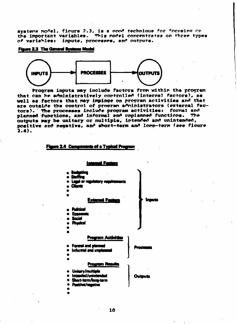
syatens ino«'el, ficure ?.3, is a ooo^ technlaue for 'ocusino OP the Inportant variables. This no<» l concentrates on three types of varia>^Ie8: inputs, procesKffs, ant* outputs.

Figise 2L3 Ths OSBSWI ^mimim wjowm

Program inputa may include factors fron withlp the program that can be administratively coptrollet* (interna) factors), as well as factora that may icqpinge on prcgran activities an< that are outside the control of prooran a«*nlnistrator8 (external fac­tors). ' The processes include progrem activities z fomal and planned functions, and informal an^ unplanned functiona. The outputs may be unitary or nnltiple, intended and unintended, positive and negative, an^ short-term ant* lore-term (see fioure 2.4).

2A Ufa

• 9aigl6a§ • Smut • iipior • Obntt

• rafiticm

# Fommlmm pmnnid * InfoiiMlmid

• UiiHmy/muhipli • Inmndid/ttRinlmidid • Slmrt-tvm/lonf>tinn

Outpum

10

.._j

After conaidering a wide range of possibls variablss* svaluators oftsn sslsct rslsvant variablea on the basis of urttat-ever data are available at the moment. According to Blalock If the obvioua atarting point ia a "caieful reading of the litera­ture, combined with a ayatematic listing of all important con­espts or variablss snd thsorstical propositions linking thsse variables." Ths following sources of information are also use­ful starting points for finding variablss.

1. proqrsm Psrsonnel. Program peraonnel may be interviewed to leSn~whether anything about the program has chsngsd or whsthsr anything unusual has happsned rseently that might explain the pro­gram onteomm. Frequently, the occurrence of soms svmn't that has been attributed to a program may be at least partially the result of soms nsw devmlopsMnt, such as a change in program funding or staffing, nsw legislation or regulatory require-msttts, or a change in the mix of program partici­pants.

2. Progppsss Reports. An analysis of a prc ram's performance tr«md may show that the effectiveness level is changing over time. Likewiae, the analy­sis may indicate periodic deviations thait can bs related to changea in the program's operating environsMnt. For example, weather conditions may affect participation in an outdoor recreational program.

3. Previous Evaluation studies. Previous eval-uatlon studies or audit reports may have already ld«itified many relevant variables. These docu­ments may be obtained from program personnel or from tne group that conducted the study. If pro­gram evaluations or audits have been perfucmad, the evaluation team should aacertain the status and examine the relevance of the prior findings. Parallels can be draim reliably only by identi­fying U&« eaaential characteristics of the present outcooM and aeeking past program outcomes that contain the same featurea. Unfortunately, it is easy to conclude that a present situation is the sams as one in the paat «dien that is not the caae, so extreme care ahould be exercised in observation, examination, and measurement.

4. Causes of Similar Effecta From Elsetdtere. Where relevant, looking at similar programs or outccstts may help to identify variables. For

in studying the potential impact of

^/Blalock [23, p. 28.

11

national health insurance legislation, it may be useful to exaad.ne the experiences of countries with similar programs. Such cases should be examined carefully, however. Similar programs may not be directly transferable, although some may point to unanticipated variables.

There are no foolproof procedures for deciding which variables to lise: nor will the evaluator Icnow for sure whether or not all the relevant variablea have been located. Seme adviae 1 / eiq>haaising those aspects' that are more or leas manip-ulable, and if feasible, those that the evaluator may deliberate­ly change for evaluation purposes. Often, however, nonmanipulable variablea are also needed to explain thoroughly the effect. Additionally, limit the relevant variables to those that have imswdiate bearing upon the current program. One should not, however, preaiaturely cloae MM search for variables. Modified and more cooiplex models may later be introduced if data do not fit the initial model.

MAKXMG ASSOMPTIOMS ABOUT CADSAI. EELAT10HSHIP8

The next step is to identify the significant relationships smong the possible causes and effect (a) being studied and con-Si^met arrow diagrasM. Thia step occurs concurrently While sslseting Uis relevant varitfslss.

As variablea and propositions are collected and consoli­dated, a useful procedure is to construct an arrow diagram of the major variables whicih also indicates ths prssumad links among them. Arrow diagrams (also called path diagraa» and flow graphs) provide a bridge bstween verbal theories and algmbraic or structural equations. With arrow diagrams, the causal model literally 1»egins to take shape and the evaluator's assumptions

visible.

Constructing an arrow diagram involvea graphically repre­senting a cause and effect hypothesis by drawing arrows from variables assumsd to be causes to variables assinssd to be effects. For example, if X is caused by both Y and Z, ich are independent of eadh other, the arrow diagram is:

j /See, for example, Suduaan [43, P- 108 and Weiss [53, p. 47.

12

An arrow shows that one variable is thought to affect the other; the direction of the arrow shows the prssunsd dirsction of Influence. Such diagrams ars read from left to right.

SosMtimss Y and Z ars assumed to l>s influencing each other, but ths specific direction is either unknown or ineonssqusntial for tho analysis. In this case, they ars connsctsd by a t%#o-hsmdsd curved arrow.

In figure 2.5 the previously discussed program eoa^onenta are arranged in an arrow diagram to show thsir causal relation­ships. Using this model as a atarting point, evaluatora arrange thmlr program variables in a similar causal orders the Internal and •x^mrnal factors are assuBMd to be direct causes of program actlvitlms, which, in turn, are assumsd direct causms of program rmoults. Furthermore, l^s program results have future impacts on ths original input factors at a later time. Inipacts on in-t e m m l factors are likely to be short-term (occurr'.ng within a ymar or t%io). Impacts on external factors are likely to bm lonq-term (occurring after S-IO years). Evaluators nssd to bs almrt for these possibls feedbacks.

Fipse 2iS Cmmri Within tha Csnimrt of s

liimtt

iwtmmi Foetom

•BudgMing

• Sttffini

OutpMtt

• lJ|N or raguitiorv

*Fonimi mid-plmHmd • Infoffliil mid Ul

ISSBL&flttI

* SiMMt*immiloii§>mmii

IMPACTS I

13 t.

When diagramming cauaal relationships, include all reasonable direct paths. For example, an internal factor may have a direct effect on the program result in addition to arr indirect effect through some program activity. Later, as the theory is tested and reviaed (using path analyais), certain links may bs dsletsd.

Figure 2.6 is a causal model of a hypothetical prison parole program. Although incomplets, it deplete the key factora being conaldered and the assuaqptions belitg made. This figure shows what is being hypothesised: parolee reintegration into society flwy be influenced by comsninity employawnt opportunities, ths parolee's environment, cosmRinity attitudes towards parolees, as well aa the parolee monitoring program itself.

When oach met of events or factora ia aeasursd, it ia pos­sible to sss %rhat %iorks and What demsn't, for %diom it works and for %diom it dossa't. If the predicted sequence of events doss mot «N>rk out, furtiimr investigation Is nssdsd.

Rim- iBwusI efslhffSwmmcBi

14

In summary, an arrow diagram is a siiqple, systematic approach for conceptualising causality. If properly used, it can furnish the evaluator with a logical way to consider the full range of variables that should be included in an explana­tion and to map out a presumed causal process.

TESTIBW A MODEL'S ADEQUACY

The "ssarch for causes" now becoanes largely one of testing ji hypothesissd associations between the selected causes and

effsct(s). As stated in chapter 1, three conditions need to be I examin-^ before concluding that X causes Y:

I 1. how X and Y are ordered in time,

2. whether X and Y are related or associated, and I

3. %ihether the relationship between X and Y is due to chance or to other factors.

In testing a causal mcd^l, these conditions must be scru-I; tlnlsmd. Ths first t«io conditions may not be troublescsM, but

how can an evaluator know tha^ all X's that affect Y directly or iadirsetly have been found? One never knows for sure. Thus,

t ths third condition requires the evaluator to anke certain sin-i; pilling amsunptlons and, in effect, admit that had another sat I of varl^lss bsttB selected and different assumptions mads, ths f caussl model might have looked quite different. Accardimg to

BlalociEt f

• •• there is nothing absolute about any parti-Cttlar modsl, nor is it true that if two models aakm uss of different variables, either ons or ^ s other must in SOSM ssnss bs "tnrong." 1/

Gmissquently, causality cannot be dssKanstrstsd from any type of empirical information. Forthsraors, setablishing a sta­tistical rslationship (correlation) bstwssn two variabioe doss not nsemssarily mssn that one variable caused the other. Corre­lation Is not causation. Nsvsrtheless, aceumulatsd correlation •vldwws can sonstimes build a credible case for a causal rela­tionship. Inferences concerning the inadequacy of causal models, if tJiey are not consistent with the data, can be awde, thereby rsqulring the snmlyst to modify the model. A technique called path analysis Is a tool for doing this.

This ch^ter presented a procedure for analysing cause and effect situations «diich focuses on building a "causal model" of

^/Blalock C13« p* 15.

15

an evaluator'a cause and effect aaaumptiona. The evaluator apecifies a finits sst of variablss, makss assumptions about causal interrelatedneaa, and tests thsir adequacy. If the resultant model ia inadequate, the evaluator modifies it until confidence is attained in ths modsl.

Ths models of causality that svaluators build are asssrtions about ths prsssnes sad ths dirsction of soma influsncs for rsla-tionships betwmsn pairs of variablss. Even with supportivs data, howmvsr, models cannot bm "proved." Empirical svidsnee can dis­prove ^^ories, but oaa asvmr "prove" aaythiag. There may be altsmativs models thst «iould provids squally plausible or better interpretations of ths availabls facts. For an svaluation's findings to bs useful in policy making, it may bs important to dsaonstrats tiiat ths most obvious altemstlvs models ars not supportsd bsttsr thsn ths andsl in question.

Even though csusal ssplanstlons can nsvmr bs absolutsly dsmonstrntsd smpirlcally, thsy srs thus still valuabls. Thsy force m svmlnstor to think about ths ceaplsxity of a task and Uie difflenity of uaderetanding the iaamr workiags of programs. Noet iwportmntly, thsy help dmvmlop the habit of sstsbllshlng a ehsia of logical assoaptions. This esn bs of grmst use in por-solng ths rmtlMial arguasnts %dilch form ths basis for evaluation, la fact, if aa saalysls is coaduetsd without a model, many impli­cit assumptions arm liluily to rsmsin hidden. Further, without a diagram, ths iaterrelatioaahipa among the various causes ars

I likely to be ignored.

16

BIBLIOGRAPHY

[l3 Blalock, H. M., Jr., Causal Inferencea in Honexperimental Research, University of North Carolina Press, Chapel Hill, worth Carolina, 1964.

[23 Blalock, H. M., Jr., Theory Construction, Prentice-Hall, Englewood Cliffs, Msw Jsrssy, 1K9.

[33 Randers, J., "Conceptualising Dynamic Models of Social SystoMs Lessons From a Study of Social Change," Ph.D. Dissertation, Massachusetts Institute of Tech­nology, Unpublishsd, Camibridge, Massachusetts, 1973.

[43 Suchman, B. A., Evaluative Rsssarch, Russsll Sags Founda­tion, Msw YOEk, 1967.

[53 Wslss, C. H., BvsluatlCTi Research, Prsntice-Hall, Englewood Cliffs, Hmw Jsrssy, 1972.

17

CHAPTER 3

PATH ANALYSIS

Path analysis is a statiatical technique for estimating the magnitude of links between variables in a causal model, it can be ussd with causal modeling, although it is not always neceasary or feasible. It provides evaluatora with information for possi­bly rsvising and better understanding the hypothesixsd relation­ships. This chapter definea path analysis and discusses data requirements and potential applications in program evaluation. 1/

WHAT IS PATH ANALYSIS?

Path analysis is a set of procedures for determining the strsngth of dirsct and indirect causal associations. It involves (1) constructing a diagram—usually part of a larger causal model« (2) calculating the magnitude of the assumsd causal associations, (3) analysing and rsvising assinqitions, and (4) interpreting the final path diagram.

It uses regression analysis to estisuits the strength of postulatsd causal rslatimshlps 2/ and providss an ovsrall estl-mats of a model's sxplanatory poM«sr. Mors importantly, path analysis hslps to idsntify spurious relationships that may need rsvising, and it permits sstimstlng ths magnituds of indirsct causal paths. Decisions can bs mads on %fhethsr ons variable in a modsl influsncss another directly, through mediating variablss, or both. Additionally, ths rslativs influsncs of direct and Indirect causal paths can bs compared. Zj

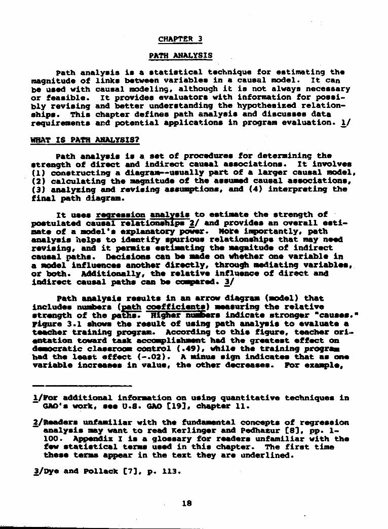
Path analysis rssults in an arrow diagram (modsl) that includes nuotoers (poth cosfficisnts) msasuring the relative strength of ths psUts. Hlghsr nuaners indicate stronger "causss." Figure 3.1 shows ths reeult of using path aaalysls to evaluate a tsaeher training program. According to this flgurs, teachsr ori­entation toward task accoaglishawnt had the greatest effect on dssMcratic classroom control (.49), %fhlls ths training program had tiie least effect (-.02). A minus sign indicates that as one varlabls inersssss in valus, the other decreases. For example.

l / ¥ o r additional Information on using quantitative techniquea in GAO'a work, see U.S. GAO [193, chaptsr 11.

2/Rsaders unfamiliar with the fundamental concepts of regression analyais may %fant to read Kerlinger and Pedhasur [83, pp* 1-100. Appendix I ia a glossary for readers unfamiliar with the few atatistical terms used in this chapter. The first time these terms appear in the text they are underlined.

2/Dye and Pollack [73, p. 113.

18

the fioure points out that olf'er teachers are Jess oriente'' toward task acconplishnenr than younger teachers (-.SO). 1/

FSgw3.1 Evshistion of Tsichsr Training

TadmrAp

ToalmrSK

CImiSa 1

-.a

- . 2 :

Trainini

1

)

- I S

1

-.02

.24

TadmrOrimimtim

Towmd Tail

Afltoimiiriii^nt

' ' i

1 *"

1.49 ^1

» \ '

Dwimiitit

Control •

.22

.20

(1S1.P.9.

DATA COLLECTION

After copstructipq a causal pio<^e] and before performjpo path analysis, an evaluator collecta r!ata. Two basic considera­tions %fhen collecting data are the i n f n m a t i e r ' s reliability an<' validity. Briefly, reliability concerns the extent to which a neasuring proce«^ure produces the aane results O P repeate<i trials. 2^/ All neasurenents contain sone amount of chance error, and "unreliability" is always present te sone extent.

i/This interpretation ^'ces not apply to "teacher sex" and "train­ing." 9iitce these variables convey I n f o m a t i o p in categories (male/female and the presence/absepce o* trainino), thev are interpreted as dunny variables. See appendix III, Test'ino the nodel's adequacy, and Pie et al. ri?i, pp. ?74-375.

2/Carmines and Zeller [5.1, p. 11.

1«

"Reliable" measurements, however, tend to be consistent when repeated. Validity, on the other hand, concerns the extent to which an "indicator measures what it is supposed to measure rather than reflecting some other phenomenon." JL/

To obtain data that accurately measure an intended phenome­non requires a well thought out research design. The following planning activities will help an evaluator collect reliable and valid data. 2^1

\ 1. Define variables precisely- so that they I can be measured. For example, "health" is i not precisely measurable, but "bed daya"

may be.

2. Determine vihat information is already available and «#hat needs to be collected.

3. Decide the costs involved, time required, and degree of precision needed.

4. Define the target population (or universe) and decide whether to collect data from the entire population or a part of it. If necessary, develop a sampling procedure.

5. Determine the frequency and tisdng-of col­lecting the data.

6. Decide Whether the data are to be collected by mail, personal interview, telephone, or other method.

7. Consider and try to control for potential sources of msasurement error—such as rsporting errors, response variance, inter­viewer and respondent bias, nonrssponse, missing data, and errora in processing the data.

8. Establish uniform proesdurss for editing, coding, and tabulating the data.

In addition to being reliable and valid, the data for path analyais should meet certain atatiatical assumptions. These include the standard ones associated with multiple regression analysis as well as some unique to path analysis. In gsnsral, theae assuisptions mean the evaluator should collect data from

I a repreaentative aample of the population and with minimum

JL/Carmines and Zeller [53, p. 16.

£/U.S. DepartsMnt of ConsMrce [183, pp* 5-7.

20

raeaaurement error. Additionally, the evaluator should specify a model in such a way that (1) there are no variablea outside the model that strongly influence any two variabl«»s in the model and (2) the causal flow is only in one direction (no feedback loops). I j Appendix II describes these assun^tions, how they affect the analysis, and what to do when they are not met.

APPLICATIOHS IH PROGRAM EVALUATION

Path analysis has specific applications in program evalua­tion. Models can be specified to ccxopare similar programs or to analyze how a program affects different segments of the popula­tion. Models are not restricted to one dependent variable, thereby, enabling multiple goals to be evaluated. In more aophisticated analyses, an evaluator can study reciprocal cause and effect and the joint effect of two or nore causes or vari­ables can be ccndsined to represent concepts that are then ana­lysed.

Program Ccxaparisons

Path analysis can compare program results. For exanqBle, an evaluator can examine a program's effect on rural and urban dwellers. To make this compariaon, one aodel is constructed, but the data are gathered from t%ro populations. Then, by examin­ing the differences between specific path coefficients 2 / the evaluator analyses the differing program results.

Specht and Warren 3 j examined a causal model (see figure 3.2) developed by Bayer 4/ that relates educational aspirations to aptitude, socioeconomTc status, and marital plans for men and women.

The path coefficienta were compared to determine whether the aodel*a structural parameters—quantities that describe a statistical population--differ between populations—in this cass men and %#OBen. The reaearch results suggssted that differences

^/The instructions in this chapter are only applicable for models ~ with ons-%#ay causal ordering, path analysis can be ussd with

models having feedback loqps; however, the procedures for cal­culating path coefficienta differ. For information on laodels with t«ro-way causal flow see Asher [13, pp* 52-61.

^/Unstandardised path coefficients need to be used becauae the ~ same variables may have different variances in different populations« Generally, standardised path coefficients are used in other applicationa. See appendix II, (Step 2. Esti­mate the path coefficients) for further information.

2/Specht and Warren [163.

4/Bayer [23*

21

did not exist between groups. For example, as shown in figure 3.2, aptitude has one of the largest relative influences on educational aspirations for both men and women. Specht and Warren were unable to reject the idea that observed differences between the two populations were due to chance.

Fiiaure3.2 Path Diaormn Rslstino Educationsi

to I. Socjoaconowic Status and Msrital Plant, by Sm

Males

0.418

Aptitude

Socioeconomic

ststus

0.167^ ^

0.081

Marital plans

_J;^5

ii

2^ ^ ^

Educational

aipirations

Fsmain

0.374 0.210

Socioeconomic

statu

Marital plans Eduational

aspirations

Soura: Adopted from Spwht and WWren (161, p. 49.

Analysing Multiple Results

One advantage path analysis has ovsr ordinary rsgression analysis is that BK>re than one dependent variable can be ana­lysed. A path diagram can be apecified with many dependent variables which represent a program's results. However, for simplicity, most causal nodsls have only one or two. By being able to specify more than one reeult, the evaluator gains a more realistic program siodel. Using multiple dependent vari­ables does not require special statistical considerations.

An example of this model is Marshall's study of the subur* banisation process. He construetsd a path diagram to examine t«ro aspects of %#hite suburbanisation: the prbbability that inner city white residents moved to the suburbs between 1965 and 1970 and the probability that %fhite newcomers to metropoli­tan areas moved to the suburbs. 1/ one hundred twelve metro­politan areas with populations 1?M>,000 or more in 1960 were analysed to determine whether iihitea were "pushed" to the

^ M a r s h a l l [113.

22

suburbs by inner city problems such as crime and race riota or "pulled" to the suburbs by their need for new homes and jobs.

The research findings indicated that whites were drawn to the suburbs between 1965 and 1970 by their need for homes and jobs rather than that they fled to the suburban areaa because of inner city problems. This suggests to policymakers that build­ing new homea and creating jobs in inner cities may aignifi-cantly change this trend.

Reciprocal Causes and Effecta

An evaluator can use path analysis to examine how one variable acts as both a cause and effect of another. In a job training program, for exan^le, unesployment levels affect pro­gram results; yet prograun activities may influence future unem-ployoMnt in that locality.

These path diagrams have arrows pointing in opposite directions (sometimes called "feedback loops"), as in this

Thsy are often more realistic than diagraiss with a one-way cauaal flow. Certain statistical assumptions, however, are no longer valid and may require collecting more data or changing thm procedures used to calculate paths, j /

If msasttresMnts are gathered at two points in time for variable A, then ordinary regressior. analyais can still be used. This laeans that A (at tiise one) is a cause of C and C is a

1 cause of A (at time t%ro). By maintaining a distinct temporal

2 order between variables A , C, and A the calculating procedures

1 2 are usually valid. However, if the data have already been

^/See the literature on structural equation modeling for further " information. Krishnan Namboodiri et al. [93, pp. 492-532;

Duncan [63, pp. 67-80.

23

collected, and only one raeaeurement ia available for A, the model can be analysed with different statiatical procedures. 1/

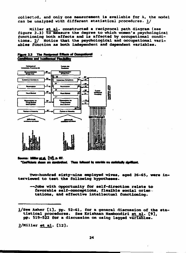
Miller et al. constructed a reciprocal path diagram (see figure 3.3) to measure the degree to %rhich women's psychological functioning both affects and is affected by occupational condi­tions. 2 j Notice that the psychological and occupational vari­ables function as both independent and dependent variables.

FlmiaU Tho EMmaof

H A £l2l.PL87.

Two-hundred sixty-nine ea^loyed wives, aged 26-65, wore in­terviewed to test ths following hypotheses.

—Jobs with opportunity for self-direct ion relate to favorable aelf-conceptions, flexible soelal orien­tations, and effective intellectual functioning.

^/See Asher [l3, pp. 52-61, for a general discussion of the sta­tiatical procedures. See Krishnan Namboodiri et al. [93, pp* 519-522 for a discussion on using lagged variables.

2/Miller et al. [123*

24

—Joba with little opportunity for self-direction relate to unfavorable aelf-conceptions, more rigid social orisntations, and less intellectual func­tioning .

The research results indicated that %rork conditions sub­stantially affset woasn's intellectual flexibility and thsir psydiologieal functioning. These fiitdlngs wsrs similar to those dsrivsd from longitudinal data for man. But no psychological variables had a atatistically aignificant rseiproeal offset on job conditions.

Joint Causes

Whan analysed, SOBM variables may have unexpectedly weak dlrset influences. Even When indirect influences are added to thsir dirsct affeeta, these variables may be statistically much wsnlrer than theory and ecnmon sense %rould lead one to anticipate. In such casss, evaluators can look for other variables that say bs interacting and affacting these variables' aignificancs. FOr ssas^le, an evaluator say find only a weak statiatical relation­ship bstwmmn length of participation in a job training program and obtaining a job. Yet, as education level increases, ths relationship between program pflurticipation and obtaining a job bseeass stronger and stronger. This situation Indicates a multi-pllcstivs relationship bst%#een the two independent variables.

In path analysis, this situation requires creating a new varlabls by multiplying togsther education level and program partlcipstl<Mi. SosMtlass thsse relationships can be anticipated and spseif led in the iaitlal aodel. At other tiaes, thess non-additive relationships can 1M ehscked by inserting in the model cross-product tsras involving all paira of indspsadent vari­ablss. y

Idmntlfyinq Underlying Concepts

Many progrsas ars too criqplex to be explained adequately by a few variables. One %Miy to include wore variables and still retain simplicity, is to combine similar HMasures. The resulting composite index is then labeled to reflect a concept common to all parts. This ccaposlts variable ahould aaaaure aa underlying charseteriatie of the Individual variables. A statistical tech­nique for grouping variablea according to uitderlying concepts is callsd factor analysis.

Factor analysis can be perfocaad by numerous statistical ccmputsr pseluigms, such as SPSS (statistical Package for the

1/For onre Infbraation on nonaddltive models, see Blalock [33, ~ pp* 91-93; BIalo6k and Blalock [43, pp* 178-186; Krishnan •smboodirl et el. [93, pp. 600-604.

25

Social Sciences) and SAS (Statistical Analysis System), which are available at GAO. / The program output is lists of factor load­ings—numbers that'show the extent to «rhich each variable relates to each factor.

This information has two uses in path analysis. First, ths variable with the highest factor loading can be considered the "best" OMasure of its factor. One variable can represent each factor in the path diagram. A second use is to combine variables into cooiposite scales representing the theoretical factors. 2l

Factor analyais should not be used "blindly" as a data reduction technique. Factor analysis assumss a model in %rhich the underlying concepts or factors ars postulated causes of the variables. Figure 3.4 illustrates the causal relationships aaxsng the variables and factors. In constructing a model using factor analysis, one assumes there are no cauae and effect rela­tions among the variables. This swans, for example, X does not

1 "causs" X just as X does not "eanss" X . Depending on the

4 3 6 variablss, this may not be an accurate assumption. 2/

FIMs* 3 . 4 Fatfi Piawan Uiini

Xi X2 X3 X4 X5 Xs X7 Xs Miller <it. ftl. included ssvsral coaiposite indicators in

ths previously discussed model (see figure 3.3), idiieh analysed women's InteAectual flexibility. In this aodel, two vari­ables^—substantive eoaqplexlty of ths job and current intellectual flexibility^—wore oMSsured by multiple indicators. Substantive oomplexity %fas aMSSured by seven indicators s hours of work with data, things, and people; complexity of work «rlth data, things.

\JSmm U.S. GAO [193, pp. 15-7 to 15-8.

2/These two uses are described in appendix III (Describe the model's ccaiponents). Methods for combining variablea are given in Runael [143, pp* 440-442 and tlie st al* [133f pp* 487-490*

2/For more information on this topic, see Sullivan and Feld-man [173*

26

and people; and the overall ccvmplexlty of the work. The index for intellectual flexibility was based on seven psychological and intelligence tests designed to measure perceptual and ide­ational flexibility.

Factor analysis can also estimate and test cooiplex causal models when measurement errors are anticipated. This method, however, is usually rscomnended only when there is a strong theory to support the model. A description of the theory and procedures involved is beyond this paper'a scops. Information about this technique can be found in statistioal literature on confirmatory factor analysis and analysis of covariance struc­tures, y Sophisticated con^uter paclcages have been developed for testing thess nxsdsls.

Path analysis is a relatively straightforward statistical technique for exaouLning causal models. With it evaluators can test causal thsoriss against available data and gain evidence to increase a B»del's credibility. The technique also allows eval­uators to sianiltaneously investigate alternative models froa which they can choose the best one. By applying path analysis, evaluators can present a clear picture of possible cause and offset interactions. They can numerically compare direct and indirect influences and see the possible impact of intervening

Ths tecdinlque, however, also has lialtations. First, since It cannot "prove" causality or establish any single model as the eorrect one, it requires starting with a sound causal theory, although this can later be modified. Second, calculating indi­rect influences becoaes cunbersoHM with too many variables. Finally, there are certain restrictions on selecting variables for a path diagram, which apply %rhenever one uses regression analysis. As long as these limitations are kept in mind, eval­uators cam use path analysis to increase their understanding of assiaad causal relationships.

1 /FOr more information, see Duncan [63, pp* 129-142; Krishnan Naoiboodiri et al. [93, pp. 555-568; and Long [103.

27

BIBLIOGRAPHY

[13 Asher, H. B., Causal Modeling, Sage Publications, Beverly Hills, California, 1976.

[23 Bayer, A. E., "Marriage Plana and Educational Aspirations,' Aaarican Journal of Sociology, volume 75, 1969, pp. 239-244.

[33 Blalock, H. M., Causal Inferences in Nonexperimental Research, University of North Carolina Press, Chapel Hill, 1964.

[43 Blalock, H. M. and A. B. Blalock, Methodology in Social Research, McGra%r^Hlll, Hew York, 1968.

[53 Carmines, E. G. and R. A. Zeller, Reliability and validity Assessawnt, Sage Publications, Beverly Hills, California, 1979.

[63 Duncan, O. D., Introduction to Structural Equation Models, Acadsmlc Press, New York^ 1975.

[73 Oys, T. R. and N. F. Pollack, "Path Analytic Models in Policy Research," Msthodoloqles for Analysing Public Policies, F. P. Scioil, Jr. and T. J. Cook (eds.), Lexington Books, Lexington, Massachusetts, 1975, pp. 113-122.

[83 Kerlingsr, F. N. and E. J. Pedhasur, Multiple Regres­sion In Behavioral Rsssarch, Bolt, Rlnehart, and Winston, Haw York, 1973.

[93 Krishnan Nambcxidlrl, H., st al.. Applied Multlvarlats Analysis and Expsriaantal Dsslgns, Mc6ra«r-Hlll, HewY^ork, 1*75. """

[103 Long, J. S., "Estimation and Hypothesis Testing in Linmsr Nodsls Containing Measursawnt Error," Sociological Methods and Research, voluaa 5, nuatoer 2, Hovssi»sr 147«, pp. i57-20«.

[113 Marshall, H., "White Movement to the Suburbss A Coapnrl-son of Eiqplanations," Aaarican Sociological Rsvlsw, voluas 44, Decsstosr 197*, pp. *75-W4.

[123 Mlllsr, J. A., et al., "wosan and Works The Psychological Infects of Occupational Conditions," Aaierlean Jour­nal of Sociology, volume 85, number 1« July 1979, pp. 66-94.

[133 Nlo. N. H. et al., SPSSt Statistical Package for the Social Sciences, McGraw-Hill. New York. 1975..

28

[143 Rumawl, R. J., Applied Factor Analysis, worthwsstern University Prsss, Evanston, Illinois, 1970.

[153 Smith, N. L. and S. L. Murray, "The Use of Path Analysis in Program Evaluation," North%«eat Regional Educational Laboratory, Portland, Oregon, Fabruary 1978.

[163 Specht, D. A. and R. D. Wsrran, "Comparing Causal Models," Socioloqlesl Methodology 1976, D. R. Hsiss (ed.), Josssy-Bass, San Francisco, California, 1975, pp. 46-82.

[173 Sttllivmn, J. L. and S. Fsldann, Multipls Indicators, Sage Piibllcstloas, Bsvsrly Hills, California, 1979.

[183 O. S. Dspsfftmsnt of Comamrcs, Statistical Policy Handbook, U. S. Gowsnmwiiit Printing Office, Washington, D.C, nay 1978.

[193 0* S. Gsnsral Aeeounting office, "Project Manual," U. S. GAO, Washington, D.C.

29

CHAPTER 4

WHEM IS CAUSAL ANALYSIS APPROPRIATE?

Gsnsrally, svaluators can uae cauaal analysis when they need to understand ccoqplsx cause and effect relationships. It providss thsm with a tool fort

—modeling coBq;>lex programa and communicating to nontechnical pe^le how pi ograms operate.

—considering alternative nndsls,

—studying both direct and indirect effects,

—incrementally revising program models, and

—developing and testing theories to understand program processss and ix^miets.

APPROPRIATE CASES

Causal analysis is applleabls in numerous svaluation situa­tions. Three general cases (sss chaptsr-2) in which evaluators can uss causal loodsling arss

— t o find out if an observed sffeet warn really due to a program or activity (ssaurchlng for csusss);

—to identil^ a program's results (finding effects); or

—to understand irtiy a program had an impact bsyond what lass sxpsetmd (analysing im­pacts).

Additionally, patii analysis can handle certain tschnleal prob-Isas—coaparing siadlar, programs or anal]^lng program effeets on diffsrsnt groups, evmluating multipls program goals, studying rseiproeal causs and offset, spselfylng joint causss, or coaA>in-ing data Into indices that rsprsssnt unaassursd conespts-that may arise in these situs^ons (see chapter 3).

Bvaluatlona, however, rarely fit neatly into predsslgnatsd categories. Many svaluations r^resmnt coniblnatlons and varia­tions of searching for causss, finding sffscts, and analysing laipacts. The following examples show how causal models could be specified in these situations and variations of the three situations. Path analysis also could be applied to any of these

1. An evaluator identifiea a "phenoaanon" and %nmts to Icnow whether and to %«hat extent

30

the program is responsible for it. In ssarching for caussn, ths svaluator*s task is to identify influences other than the program that may be responsible for the "phenonanon" and to determine their rela­tive magnitudes. Thia requires constructing a aedel with external and internal program causss.

Ths svaluator should carefully analyse possible relationships bet%raen external snd program oausss. Sines sxtemal causms are IJJcsly to bs either numerous or difficult to measurs (such as racial discriadnaticm), an evaluator may considsr emistructlng the ondsl to rsprsssnt mul­tipls, complex causss and/or effects.

2. Thm evaluator notices a discrepancy between Intsndsd and actual program results and attsmpts to find ths causss. in this sit­uation, ths evaluator identifiea and models ths direct and Indirect causss. By using path analysis to estimate the relative mag­nituds of causal paths, it may be possible to Isolats ths causes of ths discrepancy. If ths dlscrspancy is a rscsnt occurrence, ths t Is, in the piMt the program did achieve Its Intsndmd results, and "before and after"

are availabls, ths evaluator can coai-models spseif led with each data set. evaluator mmy also construct a aodel

%rlth two effects—the actual and intended program results as in the model below.

31

3. An evaluator wants to find the effects of a program. The general approach is to construct a model with multiple effects. The evaluator can emphasise one major pro­gram activity and examine its effect on program results and impacts, which are cauaally linked.

I

-•D

The evaluator can a l so construct a model with causally linked program a c t i v i t i e s and anilt ipls , unrslated e f f e c t s .

r iu|pMn MCuvnas cffacti

4. The evaluator «rants to know %^y a program had an impact other than %rtiat %ra4 expected. This could be a complex nodeling task requiring the evaluator to identify program and nonprogram processes, their interactions, and their ultimate "impact."

Examal Factors

..Extmmal f i^^inipact

32

The evaluator could examine associationa between external factors and between external factors and program proceasea for possible indirect or reciprocal influ­ences .

5. An evaluator may also identify a program's impact on an observed causal sequence of events. This involves identifying how and where a program can intervene in the causal chain and alter its consequences. This a»del nay resemble Suchman's intervening variable model (see chapter 2).

Exmmal CsaW Chnn

riKoiidition

Program Activities

This situation requires searching for causes—internally and externally—and then analysing their impact.

6. For a final variation on analyzing inq>acts, an evaluator identifies a policy's iiqpact. The evaluator identifies programs affected by the policy and analyzes the progranw* results. A general BK>del for this situation aay have this arrangement:

ErMrorwrant ;—^ft i icy ^Prcynrn >^-lnpact

LIMITATIONS

Causal analysis can be applied to many evaluation situa­tions. SoaM» causal questions that an evaluator is likely to encounter, however, caimot be answered with cauaal analysis. For exaiQ>le, an evaluator cannot generally uae the technique to predict a program's long-term effects. Causal analysis is not a forecasting technique. Likewise, it cannot find optimal values to minimize costs and maximize benefits as linear pro­gramming can.

Additionally, causal modeling does not provide a systematic way of (1) knowing if all relevant variables have been identi­fied and (2) deciding %irhich variables to use, although strong theory in a particular substantive area makes these tasks easier. Further, there is no single, correct model that explains the relationa between causes and program results. Statistical tech­niquea, such as path analysis, however, can indicate whether a

33

model is incorrect. Statistics (or science in genr-:il) can disprove theories, but can j«*»vcr "prove" them to be true. Becauae programs are dynamic, a model can only approximate a program's process at a particular time. As new data are gathered and as the program changes., the model will have to be updated.

SUMMARY

Asking causal questions is inqportant in program evaluation. Causal analysis gives evaluators a'tool for examining causs and effect relations within and from outside a program. It combines qualitative and quantitative research techniques into a highly flexible and versatile methodology that ia applicable in numer­ous situations.

Causal analysis, however, cannot be used in all situations. We have juat presented a few limitations with the technique. Nevertheless, by using the technique carefully and appropriate­ly, an evaluator can gain important understandings of the logi­cal relationships underlying or influencing programs. Finally, causal zuialysis allows an evaluator to cooraunica^e findings fully and clearly to a variety of audiences.

34

APPENDIX I APPENDIX I

GLOSSARY OF TECHNICAL TERMS

Numbers in brackets refer to the paqe where the term first appeared.

Dependent variable. A variable whose value is determined by other variables or constants in an equation or tnathenatical expression. The "effect" being explained by the causal model. [ 37]

Dummy variable. "Categorical" variable (such as "male/ female") whose components are assigned values for use in statistical analyses. For example, "male" can be assiqned a value of 0 and "female" a value of 1. [413

Factor analysis. A technique for reducing the nuinber of variables in a model. It is based on the premise that a large number of variables may be grouped into a smaller number of variables or factors, with little loss of discriminatory information. [25 ]

F-test. A statistical test of significance used for determining whether samples have been drawn froia single or different populations. [43 }

Heteroscedasticity. A condition in which the error terms of the regression equation are independently distributed, but there ars differences in the variances of the distributions associated with different fixed values of the independent variable. [41]

Homoscedasticity. A condition in which the error terms have equal variances at all points on the regression line. [41]

Independent variable. A variable used to estimate or predict another variable (the dependent variable). [37]

Interval level measurement. Level of measurement in which categories are rank ordered, with equal intervals between categories. The scale has an arbitrary zero point (such as the centigrade scale for measuring tempera­ture). [41]

Measurement error. The difference between a true value and observed value. [42]

35

APPENDIX I APPENDIX 1

Multicollinearity. A condition in which a very high correlation exists between a pair of independent variables. [42]

Nominal level measurement. Lowest level of measure­ment, which consists of classifying observa­tions into mutually exclusive categories (such as male/female). [41]

Ordinal level measurement. Level of measurement in which categories or scores are *rank ordered. One category is considered higher or lower than an adjacent category (such as ranking books from least to most popular). [41]

Parameter. A numerical characteristic relating to or describing a population which can be estimated by sampling. [21 ]

Path coefficient. Nuaierical value assigned to a path in a path diagram. It is equivalent to the standardized regression coefficient. [18]

Pearson correlation. Statistical technique used to determine the degree to which variables are linearly associated. Calculations yield a correlation coefficient (r), %rhich is a number from -1.0 to -fl.O. The extreme values ( 1) indicate that all points lie on a straigEt line. Zero indicates no linear association. [40]

Regression analysis. A procedure for relating a dependent variable to one or more independent variablea. The relation is in the form of an estimating ctquation whose purpose is to predict one variable from apecified values of others. [18]

Residual variable.. Repreaents all variablea not specified in the model that are sources of variance in the dependent variable. [42]

R-square (multiple correlation coefficient). Measures the proportion of total variation in the values of the dependent variable that are explained by the regression equation. Values range from 0.0 to 1.0. [39]

36

APPENDIX II APPENDIX II

CHECKLIST OF STEPS IN PATH ANALYSIS

Path analysis begins with a preliminary path diagram, which is similar to a causal model but with two main differences. First, a path diagram typically includes only a few "causes" (independent variables). 1/ In principle, there are no restric-tions on the nuinber of variables in a path diagram. Cost and data availability, however, generally limit the number included. Second, a path diagram is a closed system, %rhich means terms (called residual variables) are added to account for unspecified influences. 2/

The purpose of path analysis is to determine the relative atrength of cauaal relationships specified in a path diagraun. The steps to acconqplish this are:

—apecify a preliminary path diagram,

—eatimate values for the paths,

—analyze the path diagram*

—reviae the diagram (if necessary) and estimate new values, and

—interpret the final diagram.

The following checklist sunmarizes these steps. Appendix III presents an example of their application.

Step 1. Specify a Preliaiinary Path Diagram

a. Select a set of independent variables for the path diagram from the causes identified %rhile developing the causal aodel. The aost appropriate variables can be selected by using factor analysis or by choosing independent variables highly correlated with the program result or impact (the dependent variable). Both of these techniques are described in appendix III.

b. Construct a path diagram that portrays the hypothesized causal relations between variables. Path diagrams (see figure II.1) are usually dra«m with the dependent variable (the effect) placed at the far right. Variables that are not dependent upon

^/Appendix I is a glossary for readers unfamiliar with statis­tical terms.

2/Each variable with an arrow leading to it has a residual variable representing all its other "causes" not specified in the model.

37

APPENDIX II APPENDIX II

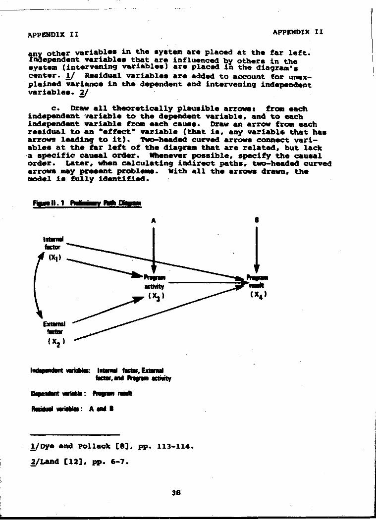
any other variables in the system are placed at the far left. Independent variablea that are influenced by others in the system (intervening variables) are placed in the diagram's center. 1/ Residual variables are added to account for unex­plained variance in the dependent and intervening independent variablea. 2/

c. Draw all theoretically plauaible arrowst from each independent variable to the dependent variable, and to each independent variable from each cauae. Draw an arrow from each reaidual to an "effect" variable (that is, any variable that has arrows leading to it). Two-headed curved arrows connect vari­ablea at the far left of the diagrwa that are related, but lack •a specific causal order. Wienever possible, specify the cauaal order. Later, %«hen calculating indirect paths, two-headed curved arro%#s nay present probleaa. With all the arrows draim, the oKSdel is fully identified.

11.1

DipmdMit arnbb;

Asid B

^/Dye and Pollack [8], pp. 113-114.

2/Land [12], pp. 6-7.

38

APPENDIX II APPFNDIX II

Step 2. Estimate the Path Coefficients

a. Convert the path diagram into a series of regression equations in which first the dependent variable is regressed against all other variables, and then the intervening variables are treated sequentially as dependent variables with their "causes" as independent variables. 1/ Values for the paths (path coefficienta) are calculated Trom these equations.

b. Solve these equations using the regression program from a coaputer package such as SPSS or SAS. 2/ The output provides the information needed to calculate coefficients fo«.' all the paths in the diagram.

—Path coefficients between the independent and dependent variables are usually atanterdized partial regression coeffic­ients. Zf

—Paths from each residual to its dependent variable have coefficients calculated by: 4/

4. 2 1 - R .

2 R (R-s^iars) is the aanunt of variance explained by the equation for the particular dependent variable.

l/For exaaqple, figure II. 1 can be represented by two equations:

X « p X - i > p X - f p A (1) 3 31 1 32 2 3a

X • p X •»- p X -I- p X > p B. (2) 4 41 1 42 2 43 3 4b

NOts that program activity (X ) acts as a dependent variable 3

in equation (1) and as a independent variable in equation (2) Bach path coefficient is identified by a symbol in the form p , in which "i" indicates where the path is going to (the iJ effect) and "j" indicates %fhere it came froa (the cause).

2/See U.S. GAO [15], pp. 15-7 to 15-8.

3 /Asher [2], pp. 23-31. Unstandardized partial regression " coefficients are used when coaparing across samples or time

periods, such as when comparing programa.

4/Ibld., p. 31.

39

APPENDIX II APPENDIX II

—Paths connecting variables that lack a specific causal ordering (two-headed curved arrows) have path coefficients calculated by the Pearson correlation, r. 1/

Each of the three methods represents the best available measure of the relationship between the "cause" and "effect" variables.

Step 3. Analyze the Model

a. Does the model account for- a sufficient amount of vari­ance (R-square) in the dependent variable that is the ultimate "effect" being examined? y If not:

—aake sure the relationships are linear.

—decide Whether to use different or additional independent variables.

—check the data for measurement error.

Convert non-linear relationships to linear ones by making appro­priate variable transformations, sudh as log transforaation or higher degree teraa. y A decision to rosove or add variablea ahould be guided by knowledge about the program. Either con­verting, raaoving, or adding variables requires reapecifying the iBOdel and recalculating the path coefficients. If these revisions fail to increase R-square, then check the data for measureoient error, such as reporting errors, response variance, and errors in processing the data.

b. Does the model violate any other atatistical assiuq>-tions? (See figure II.2)

c. Are the path coefficients directionally correct? For example, if the internal factor ia payroll staff size and the program activity is nunber of checks processed, then we expect the path coefficient to be positive (the number of checks pro­cessed increases %«hen staff size increases). If the direction is unexpected, aake sure the input data are accurate and that the progriuB is processing them correctly before interpreting the results. Don't autooatically reject counter-intuitive results, since they may indicate variables that are incorrectly placed in the andel or omitted. For exaaple, increasing staff size aay not increase output if it causes overcrowding.

^/Nie et al. [14], p. 390.

2/At the beginning of the evaluation, '£he evaluator should determine an acceptable value for R-square.

2/For a discussion on identifying appropriate variable transfor­mations see Hanushek and Jackson [9], pp. 96-101.

40

APPENDIX II APPENDIX II

Figure II.2 statistical Assumptions and Implications for Data Analysxs

AssuBg>tion

Interval level measurement

ticlty

Linear and additive relationahips

Implications and Actions

Variables are measured on an interval level scale. Including nominal and ordi­nal data in the model probably will not introduce large errors in estimating the path coefficients unless one collapses the categories too much. 1^/ Siiiply treat the data as dummy variables in the regression analyais. y

The prediction errors are equally distributed at all points on the regression line (hoao-scedasticity). This condition is identified by exaad.ning scatter diagrams of each inde­pendent variable plotted against the resid-uala. When t;he assuaqption is not met (called heteroscedasticity), a pattern emerges, such aa the one in figure II.4. y This is not a critical assumption since heteroscedastlc residuals do not bias the estimates of the regression coefficients. They do, however, biaa estinates of the standurd errors for the coefficients. If this is a problem, then another procedure (generalized least-squares) can be used for the regression conputations. 4/

Relationship between variables is linear and additive in the paraaaters. This relationship is identified by examining scatter diagrams of ths dependent variable plotted agalnat each independent variable. If the relationships do not appear reasonably linear, aake the appro­priate variable transf omations (for example, log transformations or adding interaction terma). y The violation of this assuaption can produce a low R-aquare.

1/Land [12], p. 34.

^/Lyona [13]j Nie et al. [14], pp. 273-383.

2/Beals [3], p. 344.

4/Chiswick and Chiswick [6], p. 142.

^/Aaher [2], p. 27; Blalock [5], p. 44? Wright [16], p. 190.

41

APPENDIX II APPENDIX II

Uncorrelated reaiduals

Multicolli-nearity

errors

Each residual is uncorrelated with any inde-pendent variable directly affecting the de­pendent variable upon which it acts. Pairs of residuals are uncorrelated. Reduce the likelihood of having correlated residuals by including in the aodel aa specific variables as many potentially disturbing influsncss aa poasible. Too many variables, however, will sake the a»del unwieldy, y This aasumption esn be relaxed «^en handled as in simul­taneous equation procedures, y

The correlations among variables are not so close to 1.0 that it ia difficult to asperate the effecta of one variable from another (lack of multicollinearity). Multlcolllnearity Bay occur^between independent variables in the saaa regression equation. When the correlation bettraen a pair of variables is very high (greater than .85) retain only one in the andel or use a combined index, y

Measurenants rsfleet tiie tsmm value of each variable (low aaasureaant error). Msasureaant errors produce biased estimates of the path coefficients. 4/ Rigorous quality control standards «iqn>lTed throughout the data collect tion phase will reduce the amount of measure­ment error.

• • •

• • • • '•.V

^/Dye and Pollack [8], p. 116.

2/Krlshnan Namboodiri et al. [11], pp. 522-526.

l/Al^iauser [1], p. 453.

4/Amher [2], p. 63.

42

APPCNDIX II APPENDIX II

Step 4» Revise the Model

a. Delete paths that are neither logical nor statistically significant. Two criteria are generally used to retain patha: y

—an arbitrary auLnimum path coefficient value, usually .05, and/or

—statistical significance at the .05 level (determined by the F-test). y

No path should be deleted only because its value is insignifi-eant. If there are sound theoretical reasons for retaining a path, then it should be retained.

b. Compute new path coefficienta for the reviaed model following tiie procedures in step 2.

c. Idsntify direct influences by ths single path connect­ing two variables. A direct influence is awasured by the path eosfflelsnt of that single path (aee figure II.4).

d.. Idsntify indirect paths between all pairs o£ variables using these rulssi 3/

1. Mo path say paaa through the same variable re than once.

2. Ho path aay go backward on (against the direction of) an arrow after the path has gone forward on a diffsrsnt arrow.

3* Ito path aay pass through a doubls-hsaded enrvsd arrow aore than once in a single path.

An assy %ay to apply theae rules is to iaagine trying to froa one variable to another in a path diagram without vio­

lating any rule.

The indirect paths are either cauaal (going in the direction of all arrows) or spurious (they begin by going against the diree-tlom of an arrow). In figure II.4, note that p p is not an

42 43 indirect influence bet%reen X and X because it violates rule 2.

2 3

yiMcA [12], p. 34; Kerlinger and t edhazur [10], p. 318.

2/Consult a tabls of critical F-valuss to determine the signifi-" esncs level. For an explanation of F-valuss, consult an

introductory atatistics text or Nie et al. [14]. pp. 334-340.

2/Mright [16], p. 17.

43

APPFNPIX I I

Fiiw«ll.4 CaiaulaltagDIwatmidlwiiiictPwhi APPFPPiy I I

Variables

y X 1 2

X X 1 3

X X 1 4

X X 1 5

X X 2 3

X X 4 5

Direct Path

r 12

P 31

32

P 54

Indirect Path ) Causal

r p 12 32

P P • 31 43 r p p + 12 32 43 r p 12 42 p p + 31 53 p p p + 31 43 54 r p p + 12 32 53 r p P p + 12 32 43 54 r p p 12 42 54 r p 12 31

1 •

• •

Spurious

P P + 43 53

P P P + 42 32 53 P r p p 42 12 31 53]

44

APPENDIX II APPENDIX II

e. Calculate indirect influences between all pairs of variables by multiplying the path coefficients for each indirect path segment. The sum of the indirect paths equals the total indirect influence between tvro variables. In figure 11.4, the total indirect influence of X on X is the sum of three indi-

1 4 rect paths: p p - f r p p + r p . y

31 43 12 32 43 12 42

With a cooplex model it is easy to miss paths. Indirect influences, in particular, should be checked either by reapply­ing theae rules or by using different procedures, such as Blalock*8 algorithm, y

f. For each pair of variables, add together the direct and indirect path coefficienta. This sum should approxiaate the Pearson correlation (r) between the variablea. As a rule of thuada, the t%ro values should differ by less than .05. V If they differ by a»re than .05, then too many paths aay have been deleted or a significant variable may be miaaing from the model 4/ and it should be revised.

Bigh spurious values (indicating patha that begin by going agalnat the direction of the arrow) may also indicate that the Biodel is spseif led incorrectly, y

g. Keep revising the andel until the sum of direct and in­direct influencea between moat paira^f variables equals or is close in value to their correlation. >-,

h. Cosqpute path coefficients for the final model following the procedures in step 2.

i yThka example pointa to a disadvantage of using curved arrows. '" The latter t%ro path segaants are through the tvio-headed curved arrow (r ). By including these segaants, evaluatora may be

12 overeatiaating the indirect effect of X on X , if X ia

1 4 2 actually causing a change in X (in %rtiich case these two path

1 aegaanta %rauld be spurious). Hence, it is preferable, where possible, to specify the direction of cauaation, especially aaiong variablea that can be manipulated.

2/Kzishnan Namboodiri et al. [11], pp. 461-462.

3/Kerlinger and Pedhasur [10]

4/Billings

5/Ibid.

and Wroten [4], p.

f P-

684.

45

318.

*

APPENDIX II APPENDIX II

Step 5. Interpret the Path Diagram

a. Examine the infornation contained in the final path diagram. In addition to relative values for direct and indirect influences, y path analysis provides:

—the proportion of total variation in the dependent variable (explained by the regression output, R-square).

—the portion of the dependent variable for which the independent variable is directly responsible (aaaaured by the aquared path coefficient). y

b. Evaluators can use this information to help to deter­mine if they have included a sufficient number of causes in the model (indicated by R-squars); if they have included the "best" causes y (by examining the aquared path coefficient); and if the cauaal ordering is aj^ropriats (indicated by low spurious influences). Additionally, by exaadning the influence of inter­vening vari^l>les, they may diacover high indirect effects that «rere not evident in the cauaal andel.

JL/The strength of direct and indirect paths is relative to what variables have t>een included, and is, therefore, a function of the andel*s completeness.

2/Wright [16], p. 164.

^/Peculiarities of ths sample drawn may have determined the ~ "beat" variables. With a different aample, other variables may explain more variance in the dependent variable.

46

hpjij-s;3xaJi:..v.jgjiiiBiH5i,MiigaJ

APPENDIX II APPENDIX II

BIBLIOGRAPHY

[I] Althauser, R. P., "Multicollinearity and Non-additive Regression Models," Causal Models in the Social Sciences, H. M. Blalock, Jr. (ed.), Aldine, Chicago, 1971, pp. 453-472. t

[2] Asher, H. B., Causal Modeling, Sage Publications, Beverly Hills, California, 1976.

[3] Seals, R. E., Statistics for Economists; An Introduction, I Rand McNally, Chicago, 1972.

I [4] Billings, R. S. and S. P. Wroten, "Use of Path Analysis in Industrial/Organizational Psychology: Criticisms

;' and Suggestions," Journal of implied Psychology, voluaa 63, nuniber 6, 1978, pp. 677-688.

i

[5] Blalock, H. M., Causal Inferences in Nonexperiaantal 1 Research, University of North Carolina Press, Chapel I Hill, 1^64.

[6] Chiawick, B. R. and S. J. Chiswick, Statistics and Econo-* metrics: A Problem-Solving Text, University Park

Press, Baltimore, 1975.

[7] Duncan, O. D., Introduction to Structural Equation Models, Acadeadc Preas, New York, 1975.

[8] Dye* T. R. and N. F. Pollack, "Path Analytic Models in Policy Research," Methodologies for Analyzing Public

. Policies, F. P. Scioli, Jr. and T. J. Cook (eds.), ! Lssington Books, Lexington, Massachusetts, 1975,

pp. 113-122.

[9] Hanuahek, E. A. and J. E. Jackson, Statistical Methoda I for Social Scientists, Academic Press, New York, i T97T.

i [10] Kerlinger, F. N. and E. J. Pedhazur, Multiple Regression j in Behavioral Research, Holt, Rinehart, and Winston,

New York, 1973.

[II] Krishnan NaadModiri, N. et al.. Applied Multivariate Analysis and Experimental Designs, McGra%»-Hill, New York, 1975.

[12] Land, K. C , "Principles of Path Analysis,** Sociological Methodology 1969, E. F. Borgati San Francisco, 1969, pp. 3-37. Methodology 1969, E. F. Borgatta (ed.), Jossey-Bassi ~ ~ JCISCO,

[13] Lyons, M. "Techniques for Using Ordinal Measures in Regression and Path Analysis," Sociological

47

APPENDIX II APPENDIX II

Methodology 1971, H. L. Costner (ed.), Jossey-Bass, sati Francisco, 1971, pp. 147-171.

[14] Nie, N. H. et al., SPSS: Statistical Package for the Social~Sciences, McGraw-Hill, Nev" York, 1975.

[15] U. S. General Accounting office, "Project Manual," 'J. S. GAO, Washington, D.C.

[16] Wright, S., "Path Coefficients and Path Regressions: Alternative or Complementary Concepts?" Bioaatrics, volume 16, June 1960, pp. 189-202.

48

APPENDIX III APPENDIX III

CAUSAL ANALYSIS OF PAROLE OUTCOMES

This appendix presents an example of applying causal modeling to evaluate parole outcomes. First, a sequence of behavior that might explain parole outcomes and could be altered by a parole program are hypothesized. Then a causal model using previously collected data is developed. 1/ Finally, path analy­sis is used to test the model's validity.

SELECTING VARIABLES TO STUDY

Eatablish the Evaluation's Focus

The first step in developing a causal model was to estab­lish the evaluatic's focus. This effort was constrained by two factors. First, tl. lack of a single, strong theory to explain criadnal activity or o predict parole outcomes left us without a sound theoretical O^^J. Second, the available data was limit­ed to information on 277 inmates in a maximum security peniten­tiary, y This data base did not include program information auch as funding, staff, activities, or explicit goals. There­fore, a general causal model (see figure III.l) that focussed on parolee'a behavior and background was specified.

This general cauaal model, based on Suchman's model of intervening variable analysis, y hypothesizes a social condi­tion that parole prograaa can attempt to alter. Suchaan views prograoa aa a form of intervention trying to prevent undesir­able effecta by manipulating intervening variables in a kno%#n cauaal sequence. The hypothesis is that an individual's demo­graphic and psychological characteristics influence criminal activity, which, in turn, influences parole outcoaa. Criminal activity certainly precedes parole. Does it, however, directly influence parole outcoaas? Testing this hypothesis is the focus.

l /The data base used in this chapter was collected on actual ~ parolees; however, the parole program is hypothetical. The

cauaal nndels depicted in this appendix, although realistic, do not portray a specific program.

y t h e inmates (all male) were consecutively admitted to the Ohio Penitentiary from October to December 1967. At that time, deangraphic, paychologleal, and criminal history information about the iiunates was gathered. In 1978, the information was updated from parole and criminal records. See Dynes [2] and Allen [1] for additional information.

2/Suchman [8], pp. 173-176.

49

APPENDIX I I I APPENDIX I I I

Flmiie III. 1 Qanaral Caual Modal ExplaininQ Parola Outconm

PimcondHioM Cmma Eflacm

dsnagraphic criminal » „ ! , md piydiologial • "ctiwity • outconw chinctwiitia

piroie activitlm. sidi m: .counmlinB

. ikill dfalopnwit

. community mcurity

Specify the lagortant Variables

The next step was *-o replace the general aodel with a few variables from the data baae. In theory, we could have con­structed a Biodel that included all variables. In practice, how­ever, path aitalysis assumptions (such as multicollinearity) pre­vented us from including nany variables.

Selecting the "effect" (dependent variable) waa easy; nuai-ber of parole violations was the only available measure of parole outcoaa. Reducing fifty-nine potent;al causss or pre­conditions to a few, however, was difficult. Interviewing governaant and acadeaiic experts and reviewing literature on aasessing parole outcoaas y provided little help in solving the problem, since they revealed nuaarous theories and variablss. Therefore, three statistical techniques were used to reduce the data sst, saeh producing a list of similar causes.

First, correlations between all potential independent vari­ables and the dependent variable were computed. After identify­ing 34 variables most highly correlated with the dependent vari­able, the intercorrelations between all pairs of theae variables were exaad.ned. High intercorrelations (above .85) indicated that the effecta of the two variables could not be separated (called multicollinearity) and, therefore, only one of the pair or a composite index could be used in path analysis. The four inde­pendent variables chosen had both high correlations with parole violations (the dependent variable) and low correlations with

1/Qottfredson et al. [3], pp. 43-47, conducted an extensive literature review. '

50

APPENDIX III APPENDIX III

each other, and covered the three general categories (demographic and psychological characteristics and criminal activity). These independent variables were t

—socioeconomic status,

—months in military service,

—sociopathic classification, y and

—iBonths incarcerated.

Using another statistical technique, factor analysis, y variablea with high factor loadings were c<xnbined into indices y to use aa independent variables. Ten factors were selected as a firat cut-off because they accounted for 60 percent of the variance in all the data. Those are listed in figure III.2. The nunber of factors was further reduced based on the following criteria <

—Factora 2 and 3 included siaiilar variables pertaining to criminal record from different time periods. Factor 2 was kept because it included lifetime data and it accounted for more variance.

—Factor 4 represented the dependent variable, parole violationa. It was, therefore, deleted from the list of causes.

—Factors 7, 9, and 10 were deleted because t%io criminal juatice factors had been already iden­tified (1 and 2) that accounted for more variance.

This left the following five factors*

—institutionalization (aaaaured by four incar­ceration variables),

—criminal record (arrest and conviction data).

1/Sociopathic classification is a scale ranging from normal Tndividual to hostile sociopath. The scale combines three psychological scales, number of arrests since age 18, percen­tage of life incarcerated since age 18, and number of escapes. Dynes [2], p. 46.

2/Chapter 3 (Identifying underlying concepts) defines factor aiwlyais and shows a brief example.

2/We used the procedure described by Runmel [7], pp. 440-442.

51

APPENDIX III APPBNDIX III

Figure ill.2 The First 10 Factors and Salient Variablea

Factor 1. Inatitutionalization

Incarcerations (pre 67) Months Incarcerated (pre 67) Months Incarcerated Since Age 18 (pre 67) Months Incarcerated (lifetiaa)

Factor 2. Criminal Record (pre 67 and lifetiaa)

Arrests (pre 67) Convictions (pre 67) Arrests (lifetiaa) convictions (lifetime)

Factor 3. Criminal Record (68-78)

Arrests (68-78) Convictions (68-78) Incarcerations (68-78) Parolee (68-78)

Factor 4. Reintegration

Parole Violations (pre 67) Parole and Probation Violations (pre 67) psrols Violations (lifstims)

Factor 5. Marriage

Murltal Status Tians Wsd

Factor 6. Age

Age Age at First Conviction

Factor 7. Probations

Probationa (pre 67) Probations (lifetime)

Factor 8. Alienation

Factor 9.

Factor 10.

Anoade acale Criminality Level Index

Superviaion

Ssqiervision Level

Probations (68-78)

probations (68-78)

52

iw.

APPENDIX III APPENDIX III

—marriage (narital status and times wed),

—age, and

—alienation (psychological and criminality level test scores).

Finally, for each factor between two and four variables with the highest factor loadings were identified. These were considered to be the "best" laeasures for the respective factors. This initial list of 14 variables was reduced to five by selec­ting variablea with low intercorrelations and by selecting only one variable from each factor. The third and final list of independent variablea wast

mths incarcerated,

—nuoiber of arrests,

—marital status,

—age at first conviction, and

—alienation, y

One cauaal model from each of the three lists of causes %fas construetsd. The third list produced a model that accounted for slightly more variance (22%) in the dependent variable than the othsrs (15% and 201, rsspsctively). The model produced by the third list is ussd in the resainder of the discussion.

MAKING AflSBMPTIOMS ABOUT CAUSAL RELATIONSHIPS

The five independent variables and the dependent variable were srrsngsd in ths causal asqusnee in figure 111.3. The deaK>-graphic and psychological characteriaties were aasuaad to be re­lated; however, the cauaal order betvreen them %ias not specified.

This aadel hfjiotheslses that changes in age, aarital stat­us, and alienation lead to changea in the number of lifetiaa arrests and months incarcerated, %rhich "causes" changes in the nuaber of parole violations. For example, this model asaumes that people who are young %rhen first convicted, divorced or separated, and alienated %#ould have anre lifetime arrests, spend more tiaa incarcerated, and have more parole violations than those who Iscksd thess initial characteristics. In addition, the model hypotiieaises that the deaagraphic and psychological variablea are affecting each other. For example, people who are alienated aay t>e younger when first convicted or vice versa.

^/Meaaured by the Anomie psychological test score.

i

1 53

APPENDIX III APPENDIX XII

Flgufslll.3 InitialCmmaillfladalForOaanwIniiigNrolaOutBonmB

Indipwidwt Varsbim

DanrnpiplMc

Dipadant Virlabim

I i t firm caiwicium

One liadtation to this modsl is thst ths relatimiships may be due to other factors. Because of nuaarous and sosatimes con­flicting thsoriss of criadnal behavior, %re cannot identify, anich less includs in ths aedsl, all causss of parole out<

Furthermore, the model does not include intervening program varltfBles. Bscauss we lacked data, we did not include program proceoaea that could intervene in this sequence. Program activities (such as counseliitg, drug and alcohol treataant, akill developaant, and coaanuiity necurity) and resources (includ­ing funding and ataff aize) could form a sub-model influencing parole outc

TESTING THB MODEL'S ADBQUACY

Path analysis tests the aedel's validity and determines the relative strsngth of the aasuaad causal relationships. First, a path diagram of the cauaal model was developed (see figure III.4). Residual teraa (A, B, and C) were added to account for outaide influencea. Marital status waa treated as a duaaay

54

APPENDIX III APPENDIX III

variable—married and divorced/separated, y Since all likely arrows were drawn, 2/ the diagram was fully identified.

Fiiwe lil.4 PiaMiiiinarv Path Diagwm

AftrnfifW Caiwictian

Cslculsjte the Path Coefficienta

To compute path coefficienta, each "effect" variable< arrests,, months incarcerated, and parole violationa—*ras

y i m individual «dio fell into neither of these categoriea was single. Single can be conaidered a reference category by Which the effecta of the other duaay categoriea ahould be intmspreted. For more inforaation on creating and inter­preting dummy variables see Nie et al. [5], pp. 374-375.

2/It was assumed that narital status had no direct affect on mon^s incarcerated.

55

APPENDIX III APPENDIX III

regreaaed against its "causes." y A partial listing of computer output from the SPSS regression subprogram is displayed in figure III.5.

To calculate the path coefficients, three procedures were ueed. First, the valuea for direct paths between variablea were read from the coaputer output (the "beta" y valuea in figure III.5). For example, it was determined that the path from age at first conviction to arrests had a value of -.30. V

Second, the paths from residual terma were calculated as:

-VI - R ,

2 where R is the amount of variance explained by the equation. Thus, the path between the reaidual A and arrests urast

Vl - R rf/l - . 13 « .93

Third, %dien a relationahip between two variables lacked a spseifisd causal ordsring, the association \ms deacribed by the Pearaon correlation, r. The eca puter generated thia statistic for all pairs of variables. For example, the path between age at first conviction and aarried equaled the.correlation between the t%#o (.07).

The preliminary path diagram, with path coefficients, is illustratsd in figure III.6.

Analysing ^ e Model

The prelimliuiry model was examined to detenaine if it accounted for a reasoiabls amount of variance in the dependent variable (R-squars) and to dsclds whsthsr any statistical assumptions «rere being violated.

yshxem regreasion equationa were apecified. Firat, regressing " arrests against age at first conviction, aarried, divorced/

aeparated, and alienation. Second, regressing months incarce­rated against age at firat conviction, alienation, and arreats. Third, recessing parole violationa against all o^er vari­ablea.

^/Standardised partial regression coefficients.

y t h e aiinus sign indicates that the value of one variable increases as the other decreases. The older a person is %dien first convicted, the fewer lifetime arrests likely.

56

APP2HDIX III APPENDIX III

Figure HI.5 Example of Computer Output

Arreets regreaaed agairwt age at first conviction (AGBFC), rried, divorced/separated, and alienation

It variable Arrests

R-Square « .13

Independent variablea Beta

AOBFC Married Divorced/8eparal:ed Alienation

- . 3 0 - . 0 2

.22 - . 0 6

20 .41 .07

6 .64 • Bo

Months incarcerated regreaaed against A6EFC, alienation, and arreets

it variable Mentha incarcerated

B^Sauars • .23

Independent variables

-.31 22.74 Alienation -.14 4.98 Arrests .27 18.37

Parole violationa regressed against AGEFC. aarried, divorced/ separated, alienation, arreats, months incarcerated

variable Parole violationa

B-8auare • .22

variables Beta

Divorced/Separated Alienation

iths Incarcerated

ma earjEelationa (r)

.002

.12

.003

.02

.12

.38

.002 2 .37

.002

.06 2 .86

28 .07 .

Divor­ced/ Aliena- Months Parole

AOBFC ried Sep. tion Arreata Incar. vie.

i

,

i

AflMVC

'•urarlad' ^«oieaa/8ep« AllmmsHimi i i 1 esl s MBSSBv' S B B B A •

•mv^s gia.

1.00 .07 .09

- . 1 1 - . 2 8 - . 3 7 - . 1 8

1.00 - . 6 1 - . 0 5 - . 1 7 - . 1 1 - . 1 8

1.00 .04 .20 .06 .11

1.00 - . 0 2 - . 1 1 - . 0 5

1.00 .36 .27

1.00 .43 1.00

57

pBlB=:

APPWOIX XIX APPBNDIX XII

lll.t wMiMhVmilii

This aodsl aecountsd for 22 psrcsnt of ths variation in parole violations. This %«as considsrsd acceptable, sines the rsaalning variance aay bs accounted for by the laany additional csusss of criminal bshsvior identified in the literature 1/ but itot included in ths modsl. "*

A t this tias, %rs slso rsviswsd ths statistical assumptions. Particularly, %«• sxsadnsd scatter diagraaa for linear relation­ships. Osnsrally curvllinsssr rslatlonships bstiMsn variables also eantrlbutsd to ths low variance (R-squars) si^lalnsd hy ths modsl. Sine* nuaarous varlabls transformstions fsiled to inerssse the linearity, the original untransforaad varlsblss wmrs rmtmlnsd.

1/Prlttihssd C«]. pp. 15-21.

k

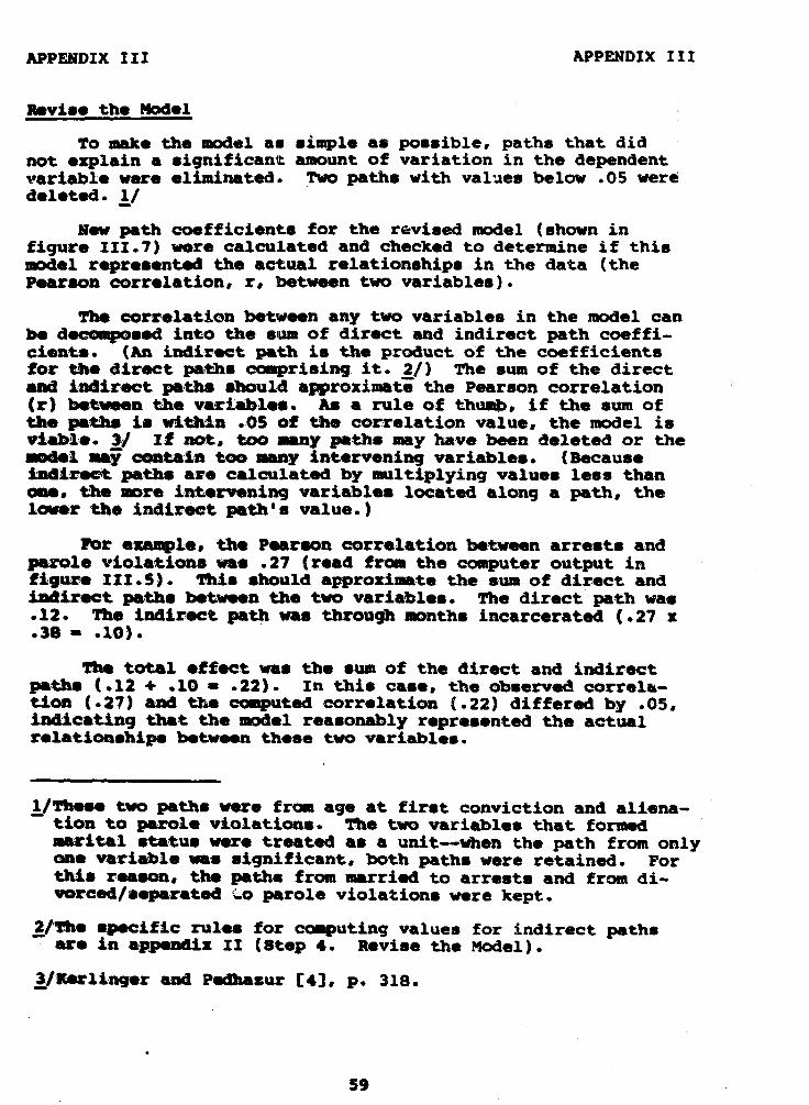
APPENDIX III APPENDIX III

Revise the Model

To aake the model as simple as possible, paths that did not explain a significant amount of variation in the dependent variable were eliminated. Two patha with values below .05 were deleted, y

New path coefficienta for the revised model (shown in figure III.7) «rore calculated and checked to determine if this model represented the actual relationahips in the data (the Pearaon correlation, r, between t%ro variables).

The correlation between any t%ro variables in the model can be decoi ioaed into the sum of direct and indirect path coeffi­cients. (An indirect path is the product of the coefficients for the direct patha cooiprising it. y y The sum of the direct and indirect paths should approximate the Pearson correlation (r) between the variables. As a rule of thumb, if the sum of the paths is wi^iln .05 of the correlation value, the model is viable. 3/ If not, too many paths may have been deleted or the modsl may contain too many intervening variablea. (Because Indlreet pat^s are calculated by aniltiplying valuea less than one, the aare interveniitg variables located along a path, the lower the indirect path's value.)

For exmnple, the Pearson correlation between arreats and parole violations was .27 (read from the computer output in figure III.5). This should approxiaate the sum of direct and Indlreet pa Uis bet%»een the t«ro variables. The direct path was .12. Ihe indirect path was through a»nths incarcerated (.27 x .38 - .10).

The total effect %ras the sum of the direct and indirect patha (.12 •«• .10 « .22). In this case, the observed correla­tion (.27) and the coa^uted correlation (.22) differed by .05, indicating that the aodel reasonably represented the actual relationships between these t%K> variables.

yttomse t%ro paths were from age at first conviction and aliena­tion to parole violationa. The two variables that formed marital status %#ere treated as a unit—when the path from only one varii^le was significant, both patha were retained. For this reason, the patha from aarried to arrests and from di­vorced/separated wo parole violationa %rare kept.

2/the specific rules for computing values for indirect paths are in appendix II (step 4. Reviae the Model).

1/Kerlinger and Pedhazur [4], p. 318.

59

APPENDIX III APPENDIX III

figum 111.7 Raviad Modal For Detrmining Parole Outcoma Using Path Analy$i$

Agi at first .convictiOR \

"•-. 30

A I 93

I .88 I

Piarole violations

A

B

In figure III.8, the entire model was decotaposed into direct, indirect, and spurious paths. (A spurious path begins by going against the causal flow.) A high spurious value may indicate that the causal order is specified incorrectly. For example, the spurious relationship between oionths incarcerated and arrests (.09) was produced by paths through age at first conviction and alienation. By reversing the causal order between age at first conviction and arrests, the spurious rela­tionship %#ould become indirect. Of course, this change %«ould be illogical and was not made. Decisions to reverse arrows should be based on theory or knowledge of time sequences; it should not be based on coefficient sizc;.

Interpret the Path Diagram

By examining the final path diagram and the decoaqposition into direct and indirect paths, knowledge about the assumed causal relationships was gained. First, it was learned that the model accounted for 22 percent of the variance in parole viola­tiona, which was considered acceptable. Second, by examining spurious influences, one could be reasonably confident that the hypothesized causal order was correct. Third, the relative strength of direct and indirect paths could be compared. For

60

APPENDIX III APPENDIX III

Figure III.8 Direct and Indirect Paths

Variables Correla­tions

lations & Arrests .27

Parole vio-lations & Incarcera­ted .43

Direct Causal Paths

Indirect Cauaal Paths

.12

.38

.10

Total Causal Paths

.22

.38

Indirect Spurious Paths

Arrests & Age

Arrests & Married

Arrests & Divorced

Arrests & Aliena­tion

Incarcera­ted & Age

Xncarcera-ted & Married

Incarcera­ted fc Divorced

Incarcera­ted & Aliena­tion

Incarcera­ted fc Arrests

Parole vio­lations & Age

Parole vio­lations & Married

Parole vio­lations k Divorced

Parole vio­lations c> Aliena­tion

-.28

-.17

.20

-.02

-.37

-.11

.06

-.11

.36

-.18

-.18

.11

-.05

-.30

-.02

.21

-.31

-.14

.27

-.12

-.003

.02

-.02

-.03

.04

-.06

-.03

.02

.05

-.18

-.02

.03

-.04

-.28

-.04

.18

.04

-.37

-.03

.02

-.09

.27

-.18

-.14

.03

-.04

,'

^

.09

.03

.05

61

APPENDIX III APPENDIX III

example, nearly half the total influence (.22) of arrests on parole violations was indirect (.10).

SUMMARY

This appendix discussed an example of using causal analysis to evaluate parole outcomes. In developing the parole outcome model, however, limitations of the technique were evident. Causal analysis cannot prove that causal relationships exist nor ensure that all relevant factors are included.

The technique pointed to the interactions among the six variables, ife know that tha five independent variables do not completely explain parole outcomes. We do not know, however, which variablea to add to the model or whether more fundamental causes are responsible for the relationships.

Nevertheless, cauaal analyais can provide valuable prog 'am inforaation. When guided by strong theory, an evaluator can conatruct a aadel with most of the significant variables-including manipulable program variables. Such a model would help evaluators and program managers to understand how the pro­gram can intervene in a hypothetical social condition and modify the coiiaequencea. Further, they could test the laodel's adequacy and ecaqpare the relative atrength of program and non-program influencea. Cauaal analyais could, thus, provide program loana-gers with useful insights for program plaxmlng and ijq>leiaenta-tion.

62

APPENDIX in APPENDIX III

BIBLIOGRAPHY

[1] Allen, ». E., "Bio-Social Correlates of Two Types of Anti-Social Sociopath," The Ohio State University, Columbus, Ohio, 1969, Ph.D. Dissertation.

[2J Dynes, P. S., "Managing the Careers of Sociopathic Felons," The Ohio State University, Columbus, Ohio, 1979, Unpublished Ph.D. Dissertation.

[3] Gottfredson, D. M., et al., Guidelines for Parole Sentenc­ing, Lexington Books, Lexington, Massachusetts, 1978.

[4] Kerlinger, F. N. and E. J. Pedhazur, Multiple Regression in Behavioral Research, Holt, Rinehart, and Winston, New York, 1973.

[5] Nie, N. H. et al., SPSS: Statistical Package for the Social Sciences, McGraw-Hill, New York, 1975.

[6] Pritchard, D. A., "Stable Predictors of Recidivism," Criminology, vol. 17, no. 1, May 1970, pp. 15-21.

[7] Rummel, R. J., Applied Factor Analysis, Northwestern University Press, Evanston, Illinois, 1970.

[8] Suchman, E. A., Evaluative Research, Russell Sage Founda­tion, New York, 1967.

(973354)

63

Rsr causal Analysist A Nathod To Identify and Test Cauae and Effect nalationships in Program Evaluations

X Please zempcnd to the following qusstions and return to Eleanor Ghelimal^, Director, Institute for Program Evaluatian.

I. HOW would you rate the job-related usefulness of this rqport?

Siiastarv- Very Little or Sana Moderate tial Great NO Utili^ UtiUty Utility Utility Utility

ChB^. It discuaaion of causality

(Sap. 2t cauaal nodaling Ch^>. 3* path analysis

4t causal analysis

H t staps in dhta aialysis

J^ppandlx I H S cuaal analysis of parole

as a whole

n n TT

n n n n

n n T7 a n n TT

TT

Vr TT

n TT TT

TT TT 77 TT

n n TT

n TT TT

rj n TT TT

2. BBS this useful on any of your inasdlate job tasks? Can you give

3. HOW halpful iidll i t lae for dasigning and understanding future eveliaticn studiss? CBn you givs an eaaaple?

4. Mat majjastiaiB do you have for iafiroving this doommnt?

5. Hhst topics vRMld you like to see discussed in future evaluatian methodology

iL-

u N D