Methodology Manual for Fresh Generation of Thematic Mapscwc.gov.in/main/HP/download/Spatial data sets Manual.pdf · 3 products. It is proposed to conduct orientation workshops for

1

1. INTRODUCTION

1.1 Hydrology Project

The Hydrology Project (HP) aims at assisting the Central Government and the participatingeight state water resources agencies in the development of valid, comprehensive, interactive,easily accessed, and user friendly data bases covering al important aspects of the hydrologicaland meteorological cycle; and to provide such data to all legitimate users involved in waterresources management. The participating States of Andhra Pradesh, Gujarat, Karnataka,Kerala, Madhya Pradesh, Maharashtra, Orissa, and Tamil Nadu have improved and expandedthe observation network, water quality laboratories and computing facilities for collection,compilation, validation and archival of point measurements of hydrometeorological andhydrological parameters.

Subsequent to the Mid Term Review of the project it is now proposed to enhance thecomponent of Geographic Information System (GIS) in HP.

1.2 GIS in Hydrology Project

Building GIS capability in Hydrology project covers

a) Hardware, GIS modules in surface and ground water data processing software, andstand-alone GIS systems

b) Generating minimum spatial data sets relevant to SW/GW hydrologyc) Georeferencing point measurementsd) Hydrometeorology/ surface water/ ground water measurements referenced to SOI map

coordinates and datume) Upgrading skill sets through training for managers and specialists

1.3 Why GIS

GIS will be used in:Customised mappingIndividual layers or combination, specific area, and as per specified map specification (scale,projection, legend, etc.)Spatial analysisAggregation of point measurements over specified area unit, interpolation and contouring,inputs for models, and theme overlayingQuerying – user specifiedBy theme, by spatial feature, by time period, and combination of above

1.4 Objective

To generate GIS data sets on select themes for integration in the Surface and Ground WaterData Centres in 8 participating States, and in the National Data Centres

2

1.5 Scope

a) State Ground Water agency will have responsibility within each state for generating anddistributing spatial data sets to State surface water agency and Central Water Commissionand Central Ground Water Board: State level Technical committee will be constituted tosupport the activity

b) Surface water and ground water agencies in each state will integrate data in respectiveData Centres

c) Central Water Commission and Central Ground Water Board will integrate data in theNational Data Centres

d) Data to be generated through outsourcing as per standard methodology before March2001

e) Spatial data sets will be in 1:50000 scale in 8 states covered by more than 2600 SOItoposheets; Scale will be 1:250000 at national level

1.6 Methodology Overview and Schedule

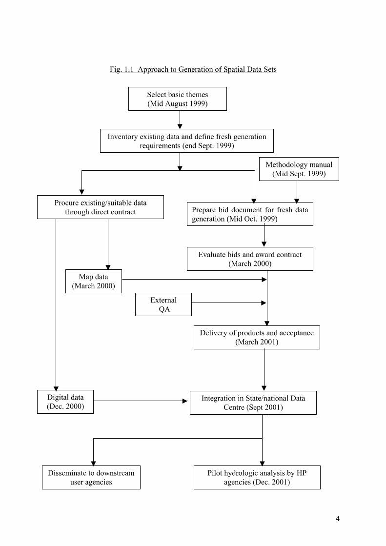
The approach to generation of spatial data sets is shown in Fig.1.1 along with the proposedtime schedule.

1.7 Procurement Process

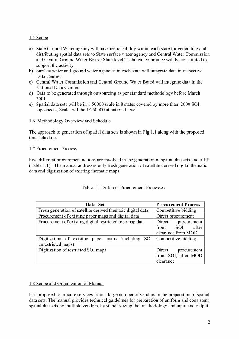
Five different procurement actions are involved in the generation of spatial datasets under HP(Table 1.1). The manual addresses only fresh generation of satellite derived digital thematicdata and digitization of existing thematic maps.

Table 1.1 Different Procurement Processes

Data Set Procurement ProcessFresh generation of satellite derived thematic digital data Competitive biddingProcurement of existing paper maps and digital data Direct procurementProcurement of existing digital restricted topomap data Direct procurement

from SOI afterclearance from MOD

Digitization of existing paper maps (including SOIunrestricted maps)

Competitive bidding

Digitization of restricted SOI maps Direct procurementfrom SOI, after MODclearance

1.8 Scope and Organization of Manual

It is proposed to procure services from a large number of vendors in the preparation of spatialdata sets. The manual provides technical guidelines for preparation of uniform and consistentspatial datasets by multiple vendors, by standardizing the methodology and input and output

3

products. It is proposed to conduct orientation workshops for successful vendors inunderstanding the manual and methodology.

The second chapter provides an overview of spatial data sets : selected themes, input data,output data, and generation methodology. This chapter also covers the spatial databaseorganization (including map tiles and TIC mark Ids) and data specifications in regard toscale, map projection, digitization accuracy, and registration accuracy between layers.Theme-wise chapters cover the classification scheme, input data specifications, methodologyflowchart, feature and attribute data coding standards, output file naming convention, internalQC and external QA, and specification for deliverable product.

Annexure 1 describes how the classification and map accuracy is estimated.

Annexure 2 describes the standard procedure for digitization.

Annexure 3 describes the internal quality control and external quality audit procedure.

Annexure 4provide details of the report accompanying each digital map tile including theQC/QA statement (map tile code, generation date, mapping accuracy, thematic accuracy,and digitization accuracy); brief description of input data, generation procedure, and outputproducts; and contact address in vendors office for future follow-up.

4

Fig. 1.1 Approach to Generation of Spatial Data Sets

Select basic themes(Mid August 1999)

Inventory existing data and define fresh generationrequirements (end Sept. 1999)

Procure existing/suitable datathrough direct contract Prepare bid document for fresh data

generation (Mid Oct. 1999)

Methodology manual(Mid Sept. 1999)

Evaluate bids and award contract(March 2000)

Map data(March 2000)

External QA

Delivery of products and acceptance(March 2001)

Integration in State/national DataCentre (Sept 2001)

Pilot hydrologic analysis by HPagencies (Dec. 2001)

Disseminate to downstreamuser agencies

Digital data(Dec. 2000)

5

2. DIRECTORY OF SPATIAL DATA

2.1 Selection of Minimum Spatial Datasets

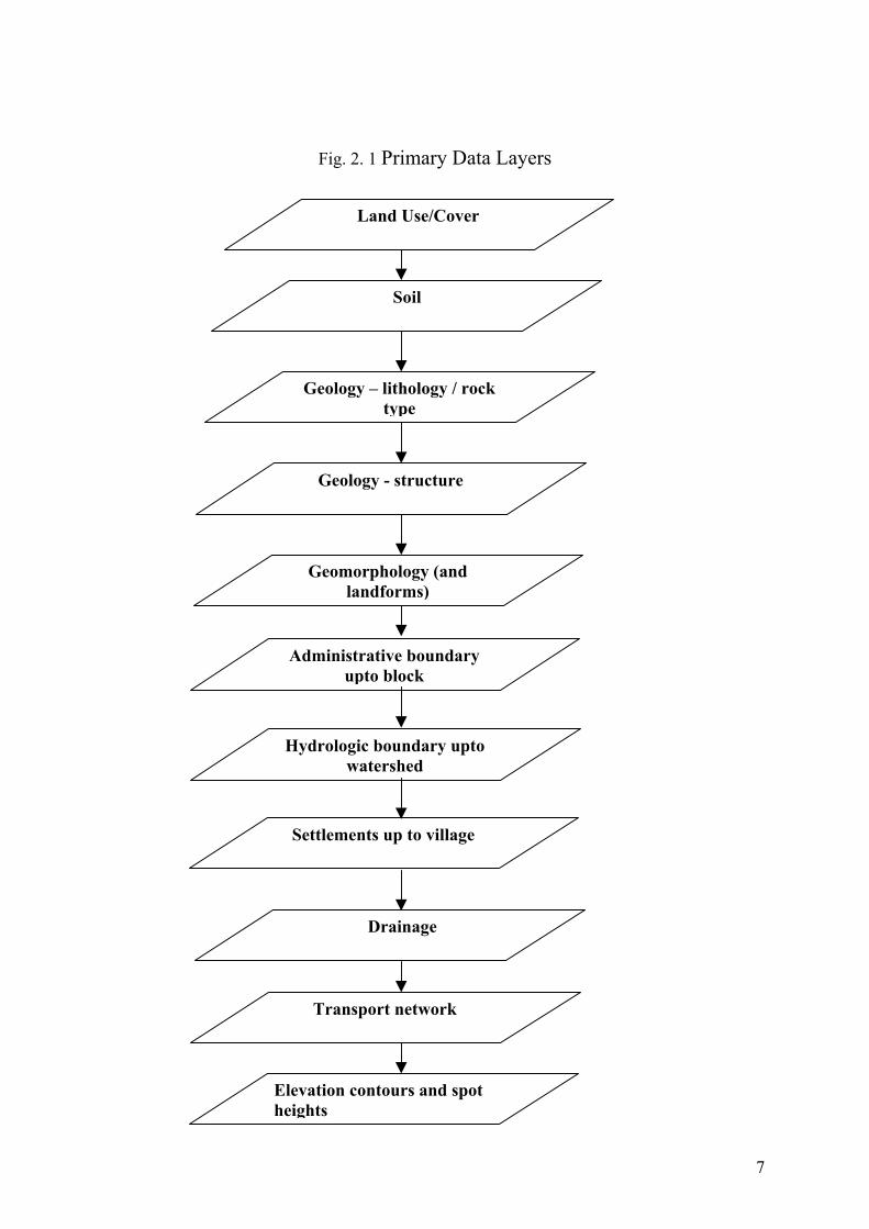
The selection of primary themes for minimum GIS data sets will be guided by the relevanceand commonality to both surface and ground water component of HP. Surface water analysisrequires a minimum set of thematic data on land use, soil, topography and drainage, whileGW analysis will additionally require spatial data on geology, geomorphology, structures,lineaments and hydrogeomorphology. General supporting data cover settlements, transportnetwork and administrative boundaries. This only constitutes a minimum spatial data set,considering the time and manpower constraints. For example data on irrigation commandareas, canal network and other water use sectors such as industries though useful will bedifficult to generate within the balance period of HP. It is envisaged that the minimum dataset will be augmented by additional spatial data sets in course of time.

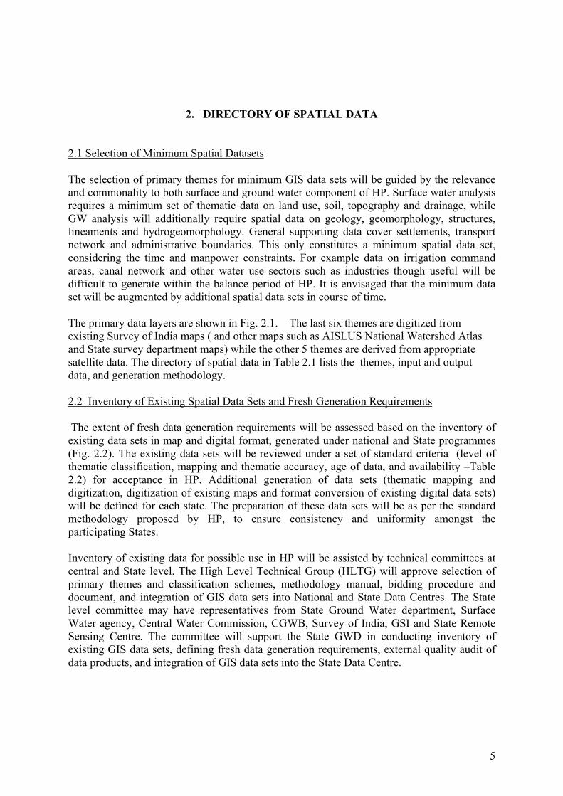
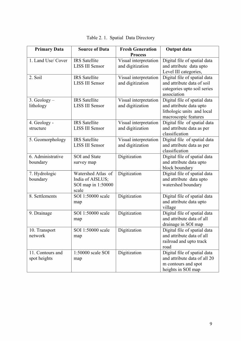
The primary data layers are shown in Fig. 2.1. The last six themes are digitized fromexisting Survey of India maps ( and other maps such as AISLUS National Watershed Atlasand State survey department maps) while the other 5 themes are derived from appropriatesatellite data. The directory of spatial data in Table 2.1 lists the themes, input and outputdata, and generation methodology.

2.2 Inventory of Existing Spatial Data Sets and Fresh Generation Requirements

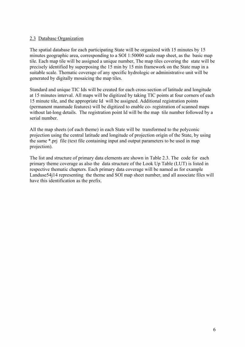
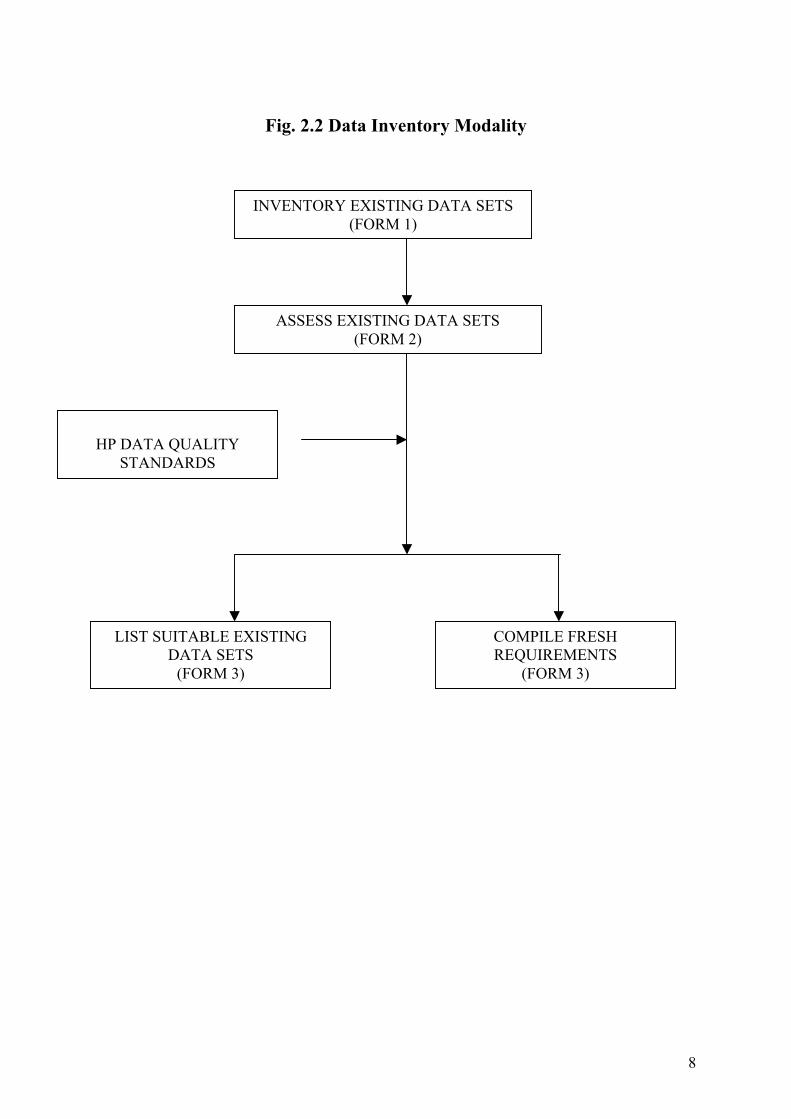
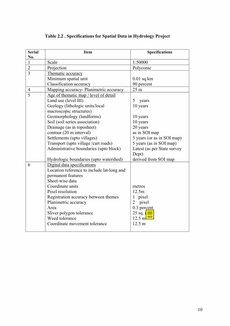
The extent of fresh data generation requirements will be assessed based on the inventory ofexisting data sets in map and digital format, generated under national and State programmes(Fig. 2.2). The existing data sets will be reviewed under a set of standard criteria (level ofthematic classification, mapping and thematic accuracy, age of data, and availability –Table2.2) for acceptance in HP. Additional generation of data sets (thematic mapping anddigitization, digitization of existing maps and format conversion of existing digital data sets)will be defined for each state. The preparation of these data sets will be as per the standardmethodology proposed by HP, to ensure consistency and uniformity amongst theparticipating States.

Inventory of existing data for possible use in HP will be assisted by technical committees atcentral and State level. The High Level Technical Group (HLTG) will approve selection ofprimary themes and classification schemes, methodology manual, bidding procedure anddocument, and integration of GIS data sets into National and State Data Centres. The Statelevel committee may have representatives from State Ground Water department, SurfaceWater agency, Central Water Commission, CGWB, Survey of India, GSI and State RemoteSensing Centre. The committee will support the State GWD in conducting inventory ofexisting GIS data sets, defining fresh data generation requirements, external quality audit ofdata products, and integration of GIS data sets into the State Data Centre.

6

2.3 Database Organization

The spatial database for each participating State will be organized with 15 minutes by 15minutes geographic area, corresponding to a SOI 1:50000 scale map sheet, as the basic maptile. Each map tile will be assigned a unique number, The map tiles covering the state will beprecisely identified by superposing the 15 min by 15 min framework on the State map in asuitable scale. Thematic coverage of any specific hydrologic or administrative unit will begenerated by digitally mosaicing the map tiles.

Standard and unique TIC Ids will be created for each cross-section of latitude and longitudeat 15 minutes interval. All maps will be digitized by taking TIC points at four corners of each15 minute tile, and the appropriate Id will be assigned. Additional registration points(permanent manmade features) will be digitized to enable co- registration of scanned mapswithout lat-long details. The registration point Id will be the map tile number followed by aserial number.

All the map sheets (of each theme) in each State will be transformed to the polyconicprojection using the central latitude and longitude of projection origin of the State, by usingthe same *.prj file (text file containing input and output parameters to be used in mapprojection).

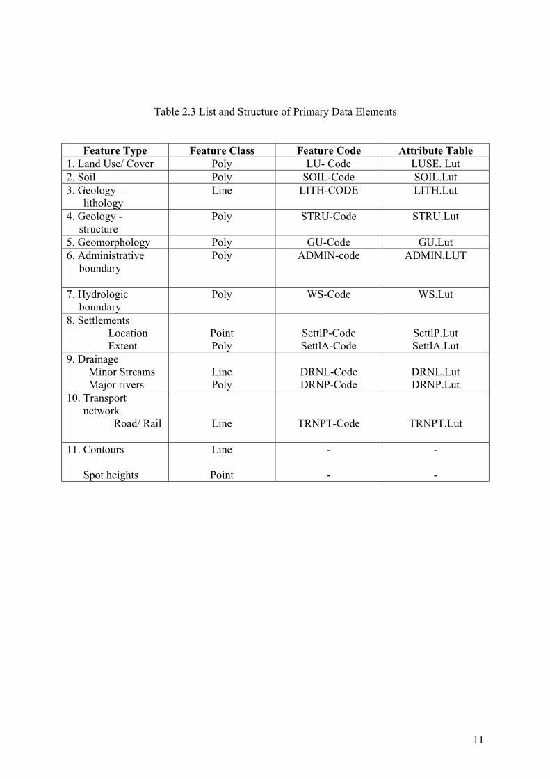
The list and structure of primary data elements are shown in Table 2.3. The code for eachprimary theme coverage as also the data structure of the Look Up Table (LUT) is listed inrespective thematic chapters. Each primary data coverage will be named as for exampleLanduse54j14 representing the theme and SOI map sheet number, and all associate files willhave this identification as the prefix.

7

Fig. 2. 1 Primary Data Layers

Land Use/Cover

Geomorphology (andlandforms)

Administrative boundaryupto block

Geology - structure

Geology – lithology / rocktype

Soil

Hydrologic boundary uptowatershed

Drainage

Transport network

Settlements up to village

Elevation contours and spotheights

8

Fig. 2.2 Data Inventory Modality

INVENTORY EXISTING DATA SETS(FORM 1)

ASSESS EXISTING DATA SETS(FORM 2)

COMPILE FRESHREQUIREMENTS

(FORM 3)

LIST SUITABLE EXISTINGDATA SETS

(FORM 3)

HP DATA QUALITYSTANDARDS

9

Table 2. 1. Spatial Data Directory

Primary Data Source of Data Fresh GenerationProcess

Output data

1. Land Use/ Cover IRS SatelliteLISS III Sensor

Visual interpretationand digitization

Digital file of spatial dataand attribute data uptoLevel III categories,

2. Soil IRS SatelliteLISS III Sensor


Digital file of spatial dataand attribute data of soilcategories upto soil seriesassociation

3. Geology –lithology

IRS SatelliteLISS III Sensor


Digital file of spatial dataand attribute data uptolithologic units and localmacroscopic features

4. Geology -structure

IRS SatelliteLISS III Sensor


Digital file of spatial dataand attribute data as perclassification

5. Geomorphology IRS SatelliteLISS III Sensor


Digital file of spatial dataand attribute data as perclassification

6. Administrativeboundary

SOI and Statesurvey map

Digitization Digital file of spatial dataand attribute data uptoblock boundary

7. Hydrologicboundary

Watershed Atlas ofIndia of AISLUS;SOI map in 1:50000scale

Digitization Digital file of spatial dataand attribute data uptowatershed boundary

8. Settlements SOI 1:50000 scalemap

Digitization Digital file of spatial dataand attribute data uptovillage

9. Drainage SOI 1:50000 scalemap

Digitization Digital file of spatial dataand attribute data of alldrainage in SOI map

10. Transportnetwork

SOI 1:50000 scalemap

Digitization Digital file of spatial dataand attribute data of allrailroad and upto trackroad

11. Contours andspot heights

1:50000 scale SOImap

Digitization Digital file of spatial dataand attribute data of all 20m contours and spotheights in SOI map

10

Table 2.2 . Specifications for Spatial Data in Hydrology Project

SerialNo.

Item Specifications

1 Scale 1:500002 Projection Polyconic3 Thematic accuracy

Minimum spatial unitClassification accuracy

0.01 sq.km90 percent

4 Mapping accuracy- Planimetric accuracy 25 m5 Age of thematic map / level of detail

Land use (level III)Geology (lithologic units/localmacroscopic structures)Geomorphology (landforms)Soil (soil series association)Drainage (as in toposheet)contour (20 m interval)Settlements (upto villages)Transport (upto village /cart roads)Administrative boundaries (upto block)

Hydrologic boundaries (upto watershed)

5 years10 years

10 years10 years20 yearsas in SOI map5 years (or as in SOI map)5 years (as in SOI map)Latest (as per State surveyDept)derived from SOI map

6 Digital data specificationsLocation reference to include lat-long andpermanent featuresSheet-wise dataCoordinate unitsPixel resolutionRegistration accuracy between themesPlanimetric accuracyAreaSliver polygon toleranceWeed toleranceCoordinate movement tolerance

metres12.5 m1 pixel2 pixel0.3 percent25 sq. m.12.5 m12.5 m

S.T.CHARI

check?

11

Table 2.3 List and Structure of Primary Data Elements

Feature Type Feature Class Feature Code Attribute Table1. Land Use/ Cover Poly LU- Code LUSE. Lut2. Soil Poly SOIL-Code SOIL.Lut3. Geology –

lithologyLine LITH-CODE LITH.Lut

4. Geology -structure

Poly STRU-Code STRU.Lut

5. Geomorphology Poly GU-Code GU.Lut6. Administrative

boundaryPoly ADMIN-code ADMIN.LUT

7. Hydrologicboundary

Poly WS-Code WS.Lut

8. Settlements Location Extent

PointPoly

SettlP-CodeSettlA-Code

SettlP.LutSettlA.Lut

9. Drainage Minor Streams Major rivers

LinePoly

DRNL-CodeDRNP-Code

DRNL.LutDRNP.Lut

10. Transportnetwork

Road/ Rail Line TRNPT-Code TRNPT.Lut

11. Contours

Spot heights

Line

Point

-

-

-

-

12

3. LAND USE / COVER

3.1 Classification System

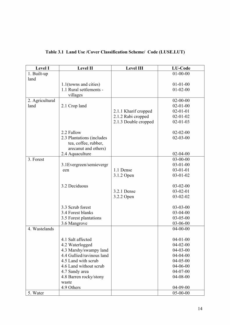
The land use / cover map will be prepared as per the classification scheme in Table 3.1. Anycategory unique to a geographic area and not included in the scheme will be labeled as‘others – Specific category”.

3.2 Input Data

- IRS LISS III geocoded False Colour Imagery (FCC) in 1:50000 scale of two timeperiods ( Kharif and Rabi season)

- SOI map in 1:50000 scale- Collateral data in the form of maps, area statistics, and reports

3.3 Methodology

The land use/cover categories will be visually interpreted (based on interpretation keydeveloped for the area) into line maps; the mapped categories may vary from map sheet tomap sheet depending on ground conditions. The interpretation process will involve referenceto collateral data to enable incorporation of features (such as forest boundaries from SOImap and from State Forest department records) and establish consistency with existing mapsand statistics ( such as existing maps on land use, wastelands and salinity affected lands and7 fold land classification statistics of State Revenue department). Delineation of Kharif andRabi crop lands and discrimination of level II and III categories will require interpretation oftwo season satellite data. All surface waterbodies (reservoirs, lakes, and tanks) will bemapped from SOI map, and updated for recent constructions with reference to recent satellitedata. The extent of waterspread will be as in SOI map, and satellite data for newconstructions. The classified map will have standard feature codes ( Table 3.1).

Field visits will be organized both for collection of ‘ground truth’ to aid and finalizeinterpretation, and to estimate the classification accuracy. The interpretation process will becontinued till the classification conforms to output data accuracy specifications (Table 2.2).

The overall classification accuracy will be estimated through ‘Kappa Coefficient’, which is ameasure of agreement between the classified map and ground conditions at a specifiednumber of sample sites (Annexure 1).

The classified map will be scanned and digitized using an appropriate scanner followingstandard procedure (Annexure 2). The Arc/Info coverage will be created and edited toremove digitization errors, and the topology will be built. The features will be labeled andcoded as defined in the LUSE.Lut (Table 3.1 and 3.2). The coverage will then betransformed into polyconic projection and coordinate system in meters. The transformationprocess will involve geometric rectification through Ground Control Points (GCPs) identifiedon the input coverage and corresponding SOI map. The HP data specification standards inTable 2.2 need to be conformed. The resulting GIS coverage will be backed up in CD andlabeled with corresponding SOI map sheet number, theme, generating agency, and generationdate.

13

Internal quality control and external quality audit will be at different critical stages ofmapping and digitization process (Annexure 3).

3.4 Output Products

Five copies of GIS coverage with appropriate file names and format (Annexure 4) in CD andtwo B/W hardcopies of thematic map will be delivered by the vendor, alongwith a report(Annexure 5) on input data used, interpretation and digitization process, internal QCstatement, and contact address for clarifications.

14

Table 3.1 Land Use /Cover Classification Scheme/ Code (LUSE.LUT)

Level I Level II Level III LU-Code1. Built-upland

1.1(towns and cities)1.1 Rural settlements -

villages

01-00-00

01-01-0001-02-00

2. Agriculturalland 2.1 Crop land

2.2 Fallow2.3 Plantations (includes

tea, coffee, rubber,arecanut and others)

2.4 Aquaculture

2.1.1 Kharif cropped2.1.2 Rabi cropped2.1.3 Double cropped

02-00-0002-01-0002-01-0102-01-0202-01-03

02-02-0002-03-00

02-04-003. Forest

3.1Evergreen/semievergreen

3.2 Deciduous

3.3 Scrub forest3.4 Forest blanks3.5 Forest plantations3.6 Mangrove

1.1 Dense3.1.2 Open

3.2.1 Dense3.2.2 Open

03-00-0003-01-0003-01-0103-01-02

03-02-0003-02-0103-02-02

03-03-0003-04-0003-05-0003-06-00

4. Wastelands

4.1 Salt affected4.2 Waterlogged4.3 Marshy/swampy land4.4 Gullied/ravinous land4.5 Land with scrub4.6 Land without scrub4.7 Sandy area4.8 Barren rocky/stonywaste4.9 Others

04-00-00

04-01-0004-02-0004-03-0004-04-0004-05-0004-06-0004-07-0004-08-00

04-09-005. Water 05-00-00

15

5.1 River/stream5.2 Reservoir/lake/tank5.3 Canal

05-01-0005-02-0005-03-00

6. Others

6.1 Inland wetlands6.2 Coastal wetlands6.3 Grass land/grazingland6.4 Salt pans

06-00-00

06-01-0006-02-0006-03-00

06-04-00

Table 3.2 Data Structure

Field Name Field Type Field Width KeyLU- Code I 8 YLev 1 C 30 NLev 2 C 30 NLev 3 C 30 N

16

4. SOILS

4.1 Classification Scheme

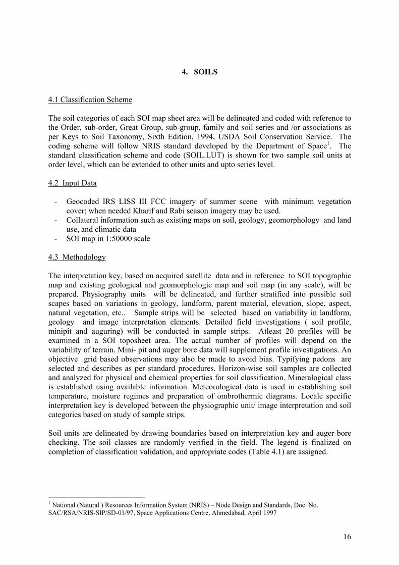
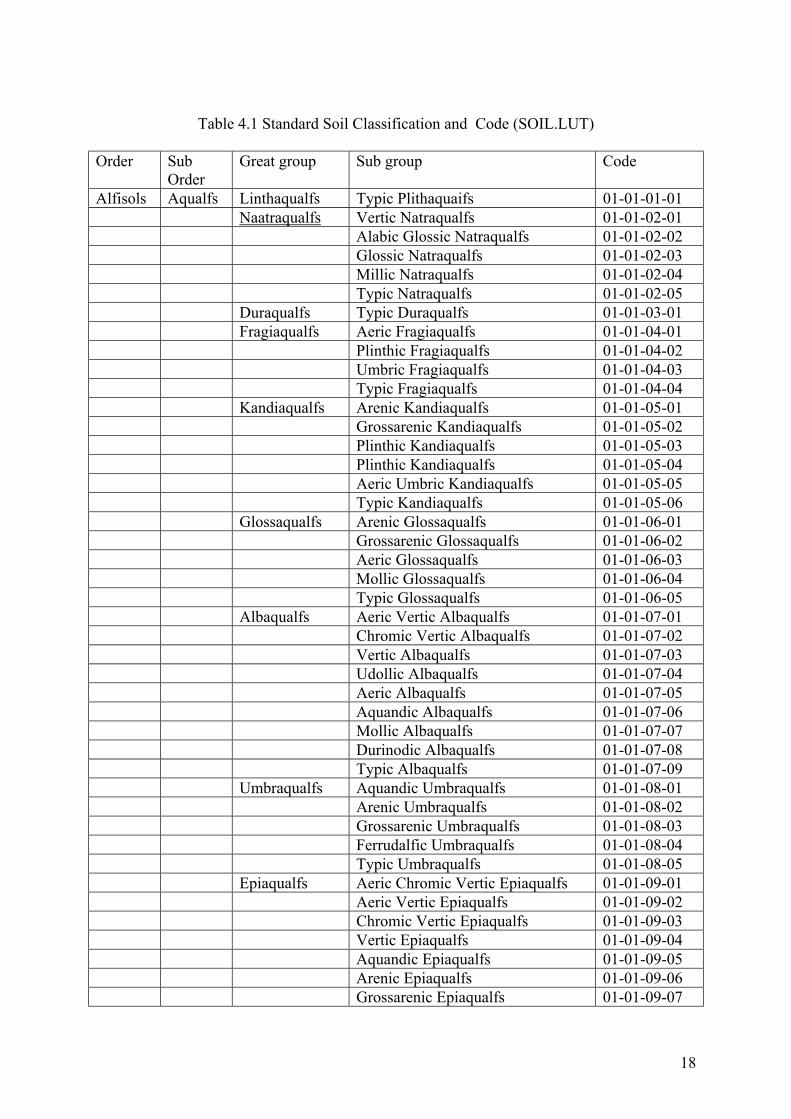
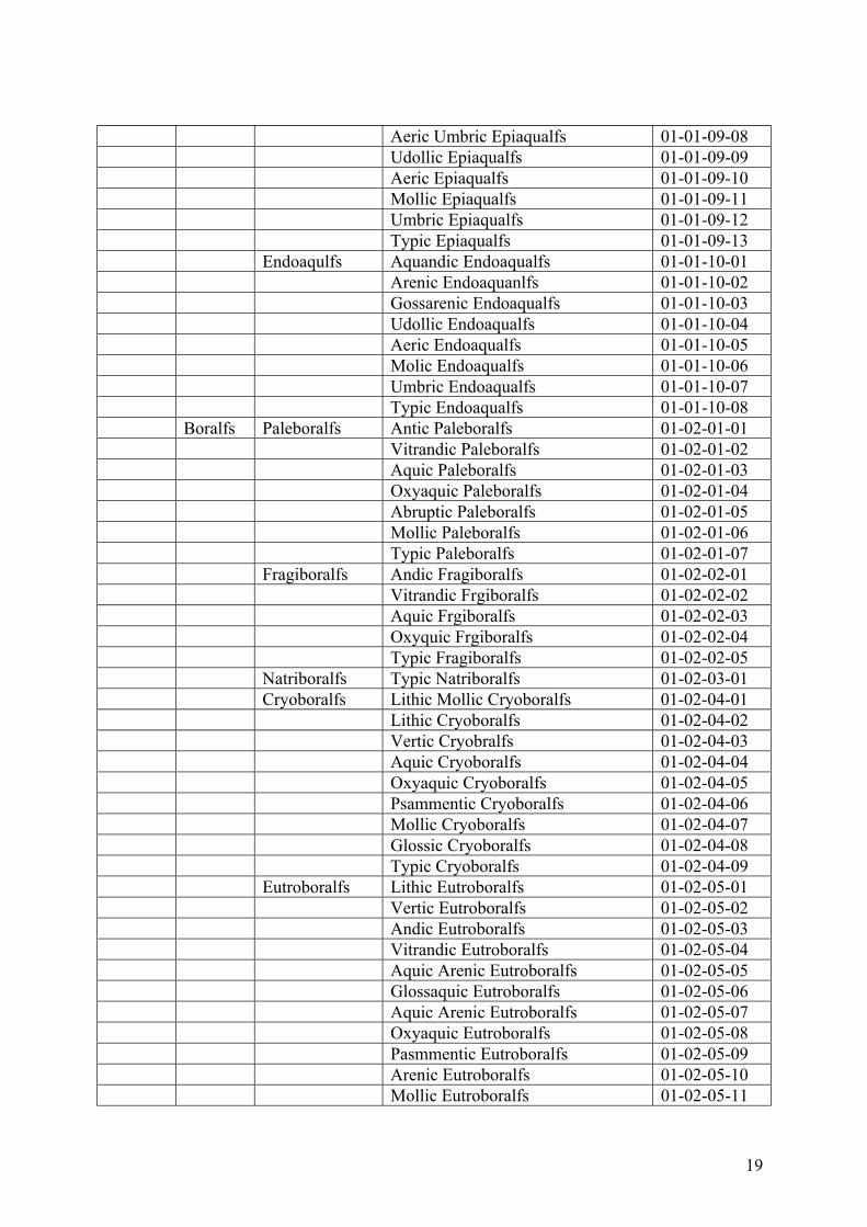
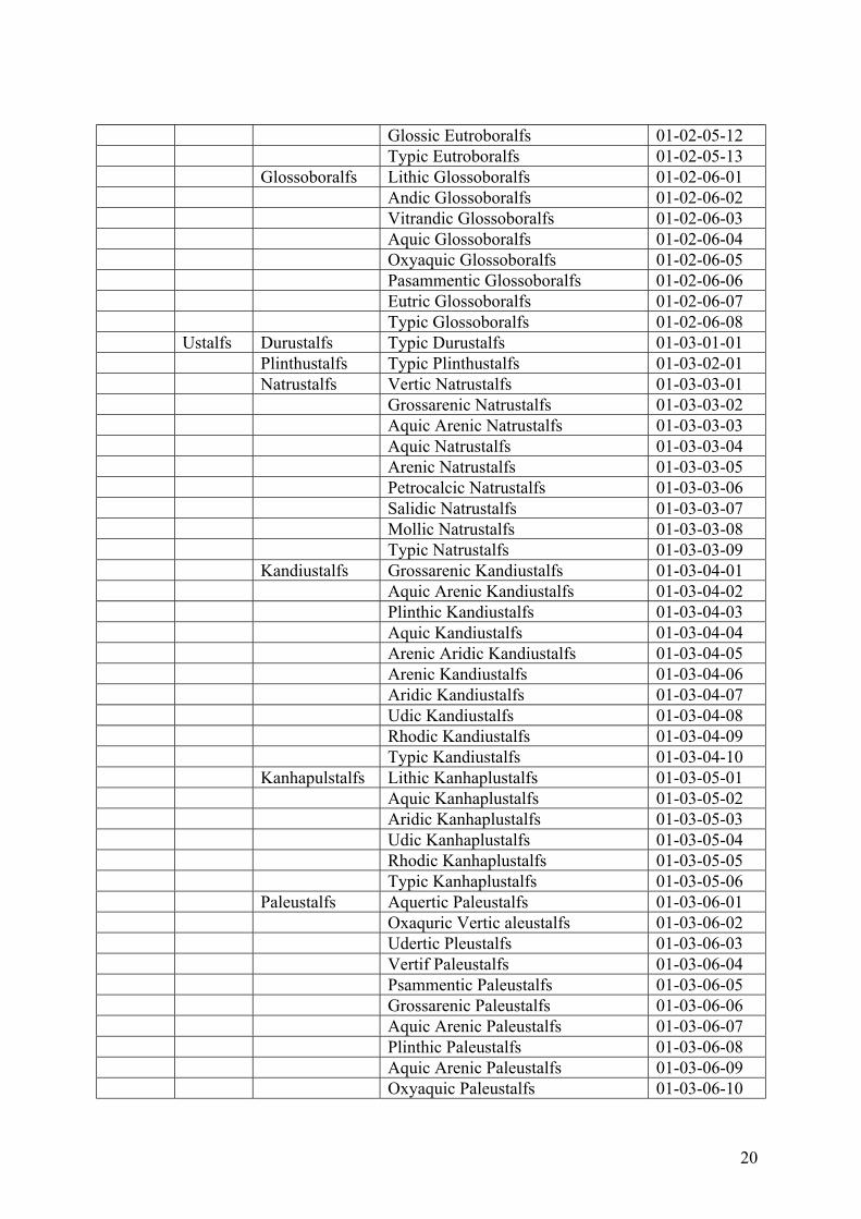
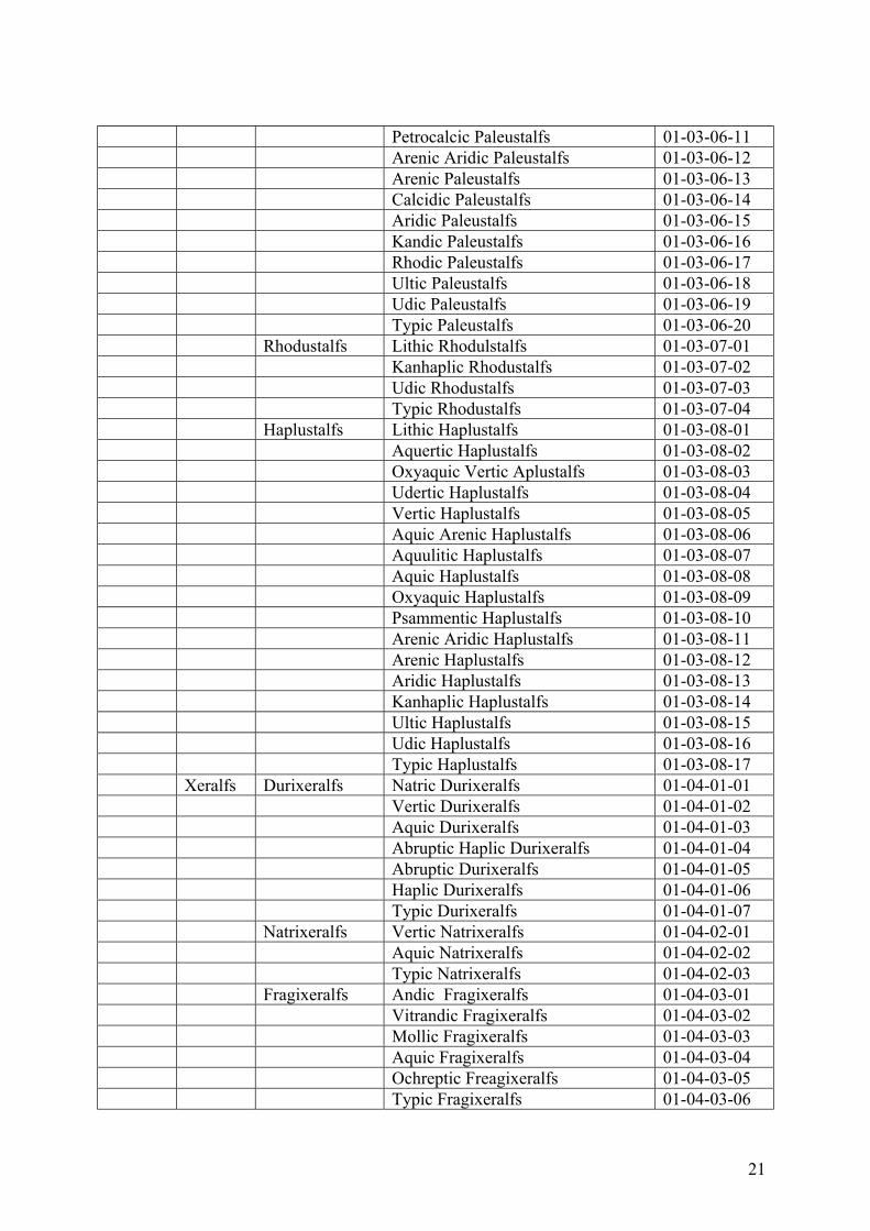
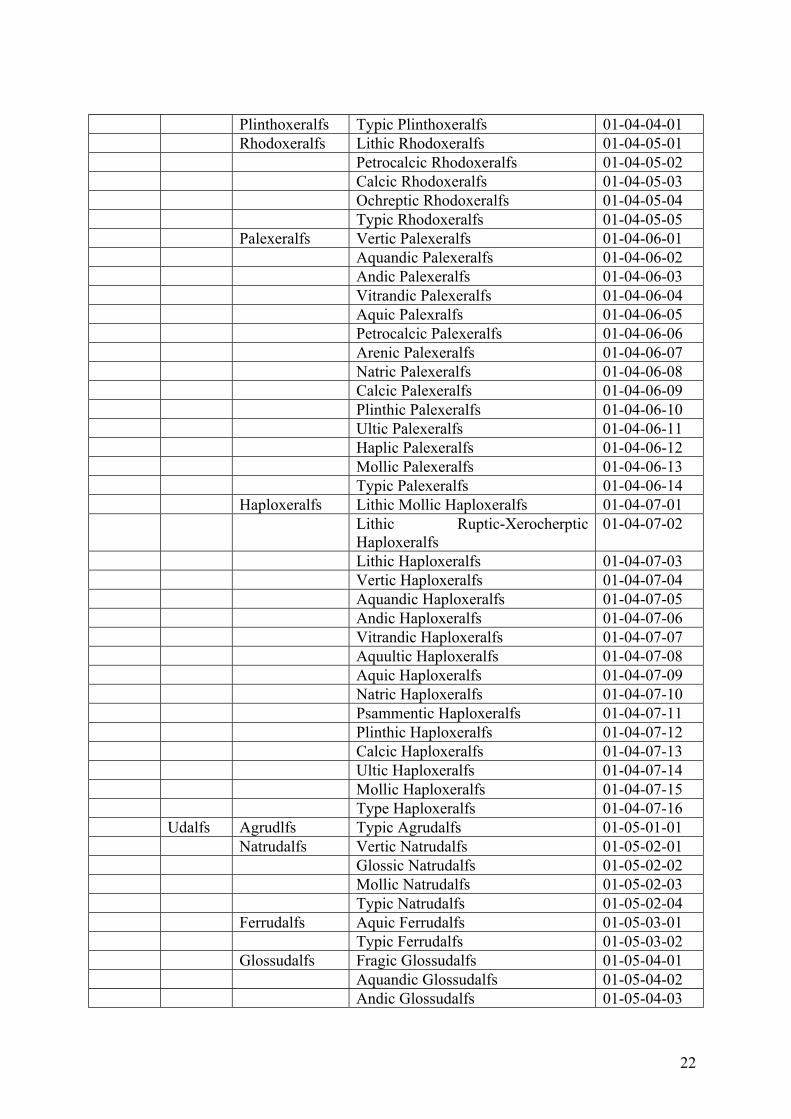
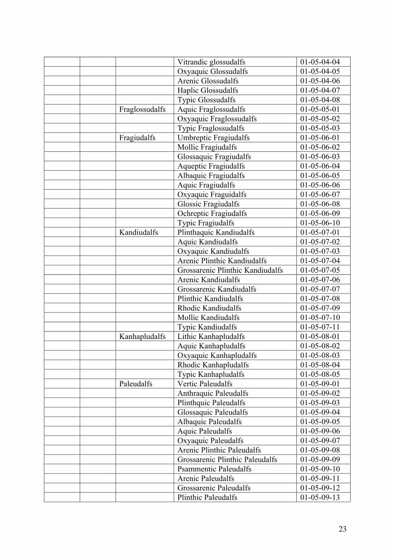
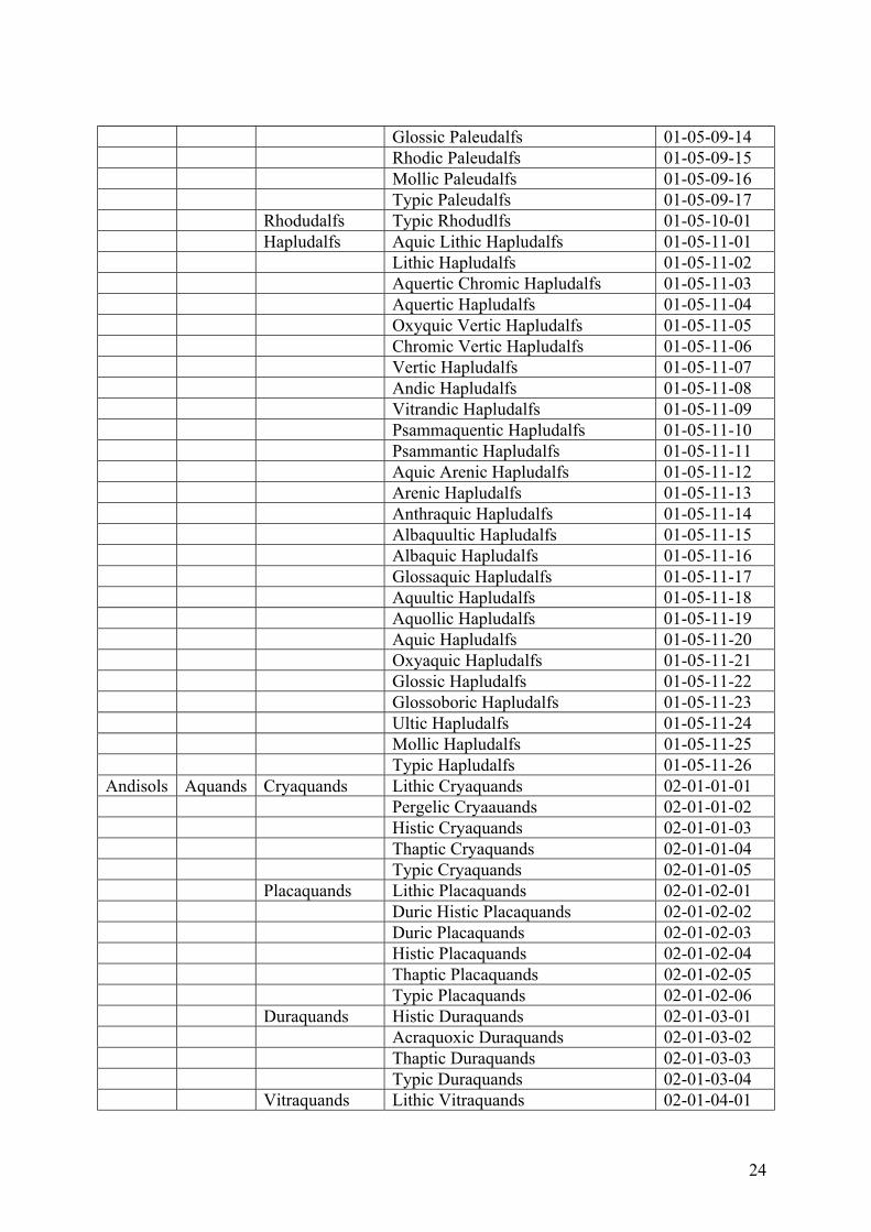
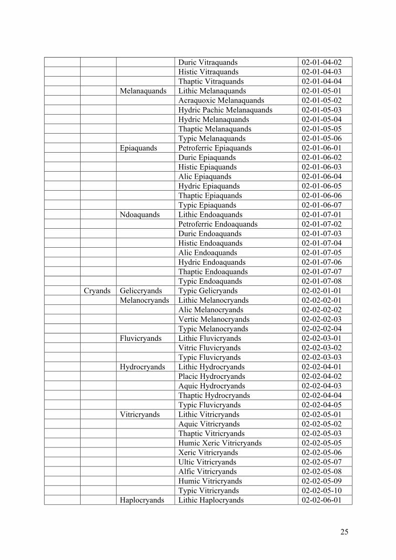
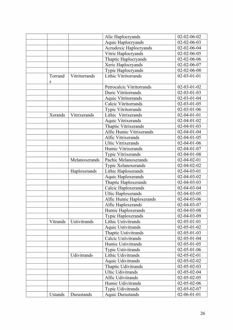
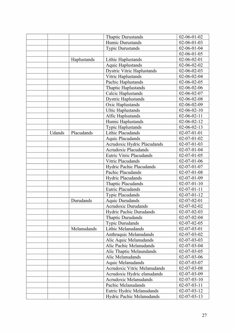
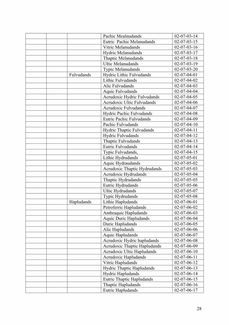
The soil categories of each SOI map sheet area will be delineated and coded with reference tothe Order, sub-order, Great Group, sub-group, family and soil series and /or associations asper Keys to Soil Taxonomy, Sixth Edition, 1994, USDA Soil Conservation Service. Thecoding scheme will follow NRIS standard developed by the Department of Space1. Thestandard classification scheme and code (SOIL.LUT) is shown for two sample soil units atorder level, which can be extended to other units and upto series level.

4.2 Input Data

- Geocoded IRS LISS III FCC imagery of summer scene with minimum vegetationcover; when needed Kharif and Rabi season imagery may be used.

- Collateral information such as existing maps on soil, geology, geomorphology and landuse, and climatic data

- SOI map in 1:50000 scale

4.3 Methodology

The interpretation key, based on acquired satellite data and in reference to SOI topographicmap and existing geological and geomorphologic map and soil map (in any scale), will beprepared. Physiography units will be delineated, and further stratified into possible soilscapes based on variations in geology, landform, parent material, elevation, slope, aspect,natural vegetation, etc.. Sample strips will be selected based on variability in landform,geology and image interpretation elements. Detailed field investigations ( soil profile,minipit and auguring) will be conducted in sample strips. Atleast 20 profiles will beexamined in a SOI toposheet area. The actual number of profiles will depend on thevariability of terrain. Mini- pit and auger bore data will supplement profile investigations. Anobjective grid based observations may also be made to avoid bias. Typifying pedons areselected and describes as per standard procedures. Horizon-wise soil samples are collectedand analyzed for physical and chemical properties for soil classification. Mineralogical classis established using available information. Meteorological data is used in establishing soiltemperature, moisture regimes and preparation of ombrothermic diagrams. Locale specificinterpretation key is developed between the physiographic unit/ image interpretation and soilcategories based on study of sample strips.

Soil units are delineated by drawing boundaries based on interpretation key and auger borechecking. The soil classes are randomly verified in the field. The legend is finalized oncompletion of classification validation, and appropriate codes (Table 4.1) are assigned.

1 National (Natural ) Resources Information System (NRIS) – Node Design and Standards, Doc. No.SAC/RSA/NRIS-SIP/SD-01/97, Space Applications Centre, Ahmedabad, April 1997

17


The classified map will be scanned and digitized using an appropriate scanner(Annexure 2).The Arc/Info coverage will be created and edited to remove digitization errors, and thetopology will be built. The features will be labeled as per codes/symbols defined in Table 4.1and 4.2.. The coverage will then be projected and transformed into polyconic projection andcoordinate system in meters. The transformation process will involve geometric rectificationthrough Ground Control Points (GCPs) identified on the input coverage and correspondingSOI map. The HP data specification standards in Table 2.2 need to be conformed. Theresulting GIS coverage will be backed up in CD and labeled with corresponding SOI mapsheet number, theme, generating agency, and generation date.

Internal quality control and external quality audit will be at different critical stages ofmapping and digitization process (Annexure 3). Additional quality assurance will includeensuring delineation of all physiographic units at the pre-field stage, study of atleast oneprofile for each prominent soil series, and post-classification validation over atleast 10percent of the area using auger bore data and road-cuts.

4.4 Output Products


18

Table 4.1 Standard Soil Classification and Code (SOIL.LUT)

Order SubOrder

Great group Sub group Code

Alfisols Aqualfs Linthaqualfs Typic Plithaquaifs 01-01-01-01Naatraqualfs Vertic Natraqualfs 01-01-02-01

Alabic Glossic Natraqualfs 01-01-02-02Glossic Natraqualfs 01-01-02-03Millic Natraqualfs 01-01-02-04Typic Natraqualfs 01-01-02-05

Duraqualfs Typic Duraqualfs 01-01-03-01Fragiaqualfs Aeric Fragiaqualfs 01-01-04-01

Plinthic Fragiaqualfs 01-01-04-02Umbric Fragiaqualfs 01-01-04-03Typic Fragiaqualfs 01-01-04-04

Kandiaqualfs Arenic Kandiaqualfs 01-01-05-01Grossarenic Kandiaqualfs 01-01-05-02Plinthic Kandiaqualfs 01-01-05-03Plinthic Kandiaqualfs 01-01-05-04Aeric Umbric Kandiaqualfs 01-01-05-05Typic Kandiaqualfs 01-01-05-06

Glossaqualfs Arenic Glossaqualfs 01-01-06-01Grossarenic Glossaqualfs 01-01-06-02Aeric Glossaqualfs 01-01-06-03Mollic Glossaqualfs 01-01-06-04Typic Glossaqualfs 01-01-06-05

Albaqualfs Aeric Vertic Albaqualfs 01-01-07-01Chromic Vertic Albaqualfs 01-01-07-02Vertic Albaqualfs 01-01-07-03Udollic Albaqualfs 01-01-07-04Aeric Albaqualfs 01-01-07-05Aquandic Albaqualfs 01-01-07-06Mollic Albaqualfs 01-01-07-07Durinodic Albaqualfs 01-01-07-08Typic Albaqualfs 01-01-07-09

Umbraqualfs Aquandic Umbraqualfs 01-01-08-01Arenic Umbraqualfs 01-01-08-02Grossarenic Umbraqualfs 01-01-08-03Ferrudalfic Umbraqualfs 01-01-08-04Typic Umbraqualfs 01-01-08-05

Epiaqualfs Aeric Chromic Vertic Epiaqualfs 01-01-09-01Aeric Vertic Epiaqualfs 01-01-09-02Chromic Vertic Epiaqualfs 01-01-09-03Vertic Epiaqualfs 01-01-09-04Aquandic Epiaqualfs 01-01-09-05Arenic Epiaqualfs 01-01-09-06Grossarenic Epiaqualfs 01-01-09-07

19

Aeric Umbric Epiaqualfs 01-01-09-08Udollic Epiaqualfs 01-01-09-09Aeric Epiaqualfs 01-01-09-10Mollic Epiaqualfs 01-01-09-11Umbric Epiaqualfs 01-01-09-12Typic Epiaqualfs 01-01-09-13

Endoaqulfs Aquandic Endoaqualfs 01-01-10-01Arenic Endoaquanlfs 01-01-10-02Gossarenic Endoaqualfs 01-01-10-03Udollic Endoaqualfs 01-01-10-04Aeric Endoaqualfs 01-01-10-05Molic Endoaqualfs 01-01-10-06Umbric Endoaqualfs 01-01-10-07Typic Endoaqualfs 01-01-10-08

Boralfs Paleboralfs Antic Paleboralfs 01-02-01-01Vitrandic Paleboralfs 01-02-01-02Aquic Paleboralfs 01-02-01-03Oxyaquic Paleboralfs 01-02-01-04Abruptic Paleboralfs 01-02-01-05Mollic Paleboralfs 01-02-01-06Typic Paleboralfs 01-02-01-07

Fragiboralfs Andic Fragiboralfs 01-02-02-01Vitrandic Frgiboralfs 01-02-02-02Aquic Frgiboralfs 01-02-02-03Oxyquic Frgiboralfs 01-02-02-04Typic Fragiboralfs 01-02-02-05

Natriboralfs Typic Natriboralfs 01-02-03-01Cryoboralfs Lithic Mollic Cryoboralfs 01-02-04-01

Lithic Cryoboralfs 01-02-04-02Vertic Cryobralfs 01-02-04-03Aquic Cryoboralfs 01-02-04-04Oxyaquic Cryoboralfs 01-02-04-05Psammentic Cryoboralfs 01-02-04-06Mollic Cryoboralfs 01-02-04-07Glossic Cryoboralfs 01-02-04-08Typic Cryoboralfs 01-02-04-09

Eutroboralfs Lithic Eutroboralfs 01-02-05-01Vertic Eutroboralfs 01-02-05-02Andic Eutroboralfs 01-02-05-03Vitrandic Eutroboralfs 01-02-05-04Aquic Arenic Eutroboralfs 01-02-05-05Glossaquic Eutroboralfs 01-02-05-06Aquic Arenic Eutroboralfs 01-02-05-07Oxyaquic Eutroboralfs 01-02-05-08Pasmmentic Eutroboralfs 01-02-05-09Arenic Eutroboralfs 01-02-05-10Mollic Eutroboralfs 01-02-05-11

20

Glossic Eutroboralfs 01-02-05-12Typic Eutroboralfs 01-02-05-13

Glossoboralfs Lithic Glossoboralfs 01-02-06-01Andic Glossoboralfs 01-02-06-02Vitrandic Glossoboralfs 01-02-06-03Aquic Glossoboralfs 01-02-06-04Oxyaquic Glossoboralfs 01-02-06-05Pasammentic Glossoboralfs 01-02-06-06Eutric Glossoboralfs 01-02-06-07Typic Glossoboralfs 01-02-06-08

Ustalfs Durustalfs Typic Durustalfs 01-03-01-01Plinthustalfs Typic Plinthustalfs 01-03-02-01Natrustalfs Vertic Natrustalfs 01-03-03-01

Grossarenic Natrustalfs 01-03-03-02Aquic Arenic Natrustalfs 01-03-03-03Aquic Natrustalfs 01-03-03-04Arenic Natrustalfs 01-03-03-05Petrocalcic Natrustalfs 01-03-03-06Salidic Natrustalfs 01-03-03-07Mollic Natrustalfs 01-03-03-08Typic Natrustalfs 01-03-03-09

Kandiustalfs Grossarenic Kandiustalfs 01-03-04-01Aquic Arenic Kandiustalfs 01-03-04-02Plinthic Kandiustalfs 01-03-04-03Aquic Kandiustalfs 01-03-04-04Arenic Aridic Kandiustalfs 01-03-04-05Arenic Kandiustalfs 01-03-04-06Aridic Kandiustalfs 01-03-04-07Udic Kandiustalfs 01-03-04-08Rhodic Kandiustalfs 01-03-04-09Typic Kandiustalfs 01-03-04-10

Kanhapulstalfs Lithic Kanhaplustalfs 01-03-05-01Aquic Kanhaplustalfs 01-03-05-02Aridic Kanhaplustalfs 01-03-05-03Udic Kanhaplustalfs 01-03-05-04Rhodic Kanhaplustalfs 01-03-05-05Typic Kanhaplustalfs 01-03-05-06

Paleustalfs Aquertic Paleustalfs 01-03-06-01Oxaquric Vertic aleustalfs 01-03-06-02Udertic Pleustalfs 01-03-06-03Vertif Paleustalfs 01-03-06-04Psammentic Paleustalfs 01-03-06-05Grossarenic Paleustalfs 01-03-06-06Aquic Arenic Paleustalfs 01-03-06-07Plinthic Paleustalfs 01-03-06-08Aquic Arenic Paleustalfs 01-03-06-09Oxyaquic Paleustalfs 01-03-06-10

21

Petrocalcic Paleustalfs 01-03-06-11Arenic Aridic Paleustalfs 01-03-06-12Arenic Paleustalfs 01-03-06-13Calcidic Paleustalfs 01-03-06-14Aridic Paleustalfs 01-03-06-15Kandic Paleustalfs 01-03-06-16Rhodic Paleustalfs 01-03-06-17Ultic Paleustalfs 01-03-06-18Udic Paleustalfs 01-03-06-19Typic Paleustalfs 01-03-06-20

Rhodustalfs Lithic Rhodulstalfs 01-03-07-01Kanhaplic Rhodustalfs 01-03-07-02Udic Rhodustalfs 01-03-07-03Typic Rhodustalfs 01-03-07-04

Haplustalfs Lithic Haplustalfs 01-03-08-01Aquertic Haplustalfs 01-03-08-02Oxyaquic Vertic Aplustalfs 01-03-08-03Udertic Haplustalfs 01-03-08-04Vertic Haplustalfs 01-03-08-05Aquic Arenic Haplustalfs 01-03-08-06Aquulitic Haplustalfs 01-03-08-07Aquic Haplustalfs 01-03-08-08Oxyaquic Haplustalfs 01-03-08-09Psammentic Haplustalfs 01-03-08-10Arenic Aridic Haplustalfs 01-03-08-11Arenic Haplustalfs 01-03-08-12Aridic Haplustalfs 01-03-08-13Kanhaplic Haplustalfs 01-03-08-14Ultic Haplustalfs 01-03-08-15Udic Haplustalfs 01-03-08-16Typic Haplustalfs 01-03-08-17

Xeralfs Durixeralfs Natric Durixeralfs 01-04-01-01Vertic Durixeralfs 01-04-01-02Aquic Durixeralfs 01-04-01-03Abruptic Haplic Durixeralfs 01-04-01-04Abruptic Durixeralfs 01-04-01-05Haplic Durixeralfs 01-04-01-06Typic Durixeralfs 01-04-01-07

Natrixeralfs Vertic Natrixeralfs 01-04-02-01Aquic Natrixeralfs 01-04-02-02Typic Natrixeralfs 01-04-02-03

Fragixeralfs Andic Fragixeralfs 01-04-03-01Vitrandic Fragixeralfs 01-04-03-02Mollic Fragixeralfs 01-04-03-03Aquic Fragixeralfs 01-04-03-04Ochreptic Freagixeralfs 01-04-03-05Typic Fragixeralfs 01-04-03-06

22

Plinthoxeralfs Typic Plinthoxeralfs 01-04-04-01Rhodoxeralfs Lithic Rhodoxeralfs 01-04-05-01

Petrocalcic Rhodoxeralfs 01-04-05-02Calcic Rhodoxeralfs 01-04-05-03Ochreptic Rhodoxeralfs 01-04-05-04Typic Rhodoxeralfs 01-04-05-05

Palexeralfs Vertic Palexeralfs 01-04-06-01Aquandic Palexeralfs 01-04-06-02Andic Palexeralfs 01-04-06-03Vitrandic Palexeralfs 01-04-06-04Aquic Palexralfs 01-04-06-05Petrocalcic Palexeralfs 01-04-06-06Arenic Palexeralfs 01-04-06-07Natric Palexeralfs 01-04-06-08Calcic Palexeralfs 01-04-06-09Plinthic Palexeralfs 01-04-06-10Ultic Palexeralfs 01-04-06-11Haplic Palexeralfs 01-04-06-12Mollic Palexeralfs 01-04-06-13Typic Palexeralfs 01-04-06-14

Haploxeralfs Lithic Mollic Haploxeralfs 01-04-07-01Lithic Ruptic-XerocherpticHaploxeralfs

01-04-07-02

Lithic Haploxeralfs 01-04-07-03Vertic Haploxeralfs 01-04-07-04Aquandic Haploxeralfs 01-04-07-05Andic Haploxeralfs 01-04-07-06Vitrandic Haploxeralfs 01-04-07-07Aquultic Haploxeralfs 01-04-07-08Aquic Haploxeralfs 01-04-07-09Natric Haploxeralfs 01-04-07-10Psammentic Haploxeralfs 01-04-07-11Plinthic Haploxeralfs 01-04-07-12Calcic Haploxeralfs 01-04-07-13Ultic Haploxeralfs 01-04-07-14Mollic Haploxeralfs 01-04-07-15Type Haploxeralfs 01-04-07-16

Udalfs Agrudlfs Typic Agrudalfs 01-05-01-01Natrudalfs Vertic Natrudalfs 01-05-02-01

Glossic Natrudalfs 01-05-02-02Mollic Natrudalfs 01-05-02-03Typic Natrudalfs 01-05-02-04

Ferrudalfs Aquic Ferrudalfs 01-05-03-01Typic Ferrudalfs 01-05-03-02

Glossudalfs Fragic Glossudalfs 01-05-04-01Aquandic Glossudalfs 01-05-04-02Andic Glossudalfs 01-05-04-03

23

Vitrandic glossudalfs 01-05-04-04Oxyaquic Glossudalfs 01-05-04-05Arenic Glossudalfs 01-05-04-06Haplic Glossudalfs 01-05-04-07Typic Glossudalfs 01-05-04-08

Fraglossudalfs Aquic Fraglossudalfs 01-05-05-01Oxyaquic Fraglossudalfs 01-05-05-02Typic Fraglossudalfs 01-05-05-03

Fragiudalfs Umbreptic Fragiudalfs 01-05-06-01Mollic Fragiudalfs 01-05-06-02Glossaquic Fragiudalfs 01-05-06-03Aqueptic Fragiudalfs 01-05-06-04Albaquic Fragiudalfs 01-05-06-05Aquic Fragiudalfs 01-05-06-06Oxyaquic Fraguidalfs 01-05-06-07Glossic Fragiudalfs 01-05-06-08Ochreptic Fragiudalfs 01-05-06-09Typic Fragiudalfs 01-05-06-10

Kandiudalfs Plinthaquic Kandiudalfs 01-05-07-01Aquic Kandiudalfs 01-05-07-02Oxyaquic Kandiudalfs 01-05-07-03Arenic Plinthic Kandiudalfs 01-05-07-04Grossarenic Plinthic Kandiudalfs 01-05-07-05Arenic Kandiudalfs 01-05-07-06Grossarenic Kandiudalfs 01-05-07-07Plinthic Kandiudalfs 01-05-07-08Rhodic Kandiudalfs 01-05-07-09Mollic Kandiudalfs 01-05-07-10Typic Kandiudalfs 01-05-07-11

Kanhapludalfs Lithic Kanhapludalfs 01-05-08-01Aquic Kanhapludalfs 01-05-08-02Oxyaquic Kanhapludalfs 01-05-08-03Rhodic Kanhapludalfs 01-05-08-04Typic Kanhapludalfs 01-05-08-05

Paleudalfs Vertic Paleudalfs 01-05-09-01Anthraquic Paleudalfs 01-05-09-02Plinthquic Paleudalfs 01-05-09-03Glossaquic Paleudalfs 01-05-09-04Albaquic Paleudalfs 01-05-09-05Aquic Paleudalfs 01-05-09-06Oxyaquic Paleudalfs 01-05-09-07Arenic Plinthic Paleudalfs 01-05-09-08Grossarenic Plinthic Paleudalfs 01-05-09-09Psammentic Paleudalfs 01-05-09-10Arenic Paleudalfs 01-05-09-11Grossarenic Paleudalfs 01-05-09-12Plinthic Paleudalfs 01-05-09-13

24

Glossic Paleudalfs 01-05-09-14Rhodic Paleudalfs 01-05-09-15Mollic Paleudalfs 01-05-09-16Typic Paleudalfs 01-05-09-17

Rhodudalfs Typic Rhodudlfs 01-05-10-01Hapludalfs Aquic Lithic Hapludalfs 01-05-11-01

Lithic Hapludalfs 01-05-11-02Aquertic Chromic Hapludalfs 01-05-11-03Aquertic Hapludalfs 01-05-11-04Oxyquic Vertic Hapludalfs 01-05-11-05Chromic Vertic Hapludalfs 01-05-11-06Vertic Hapludalfs 01-05-11-07Andic Hapludalfs 01-05-11-08Vitrandic Hapludalfs 01-05-11-09Psammaquentic Hapludalfs 01-05-11-10Psammantic Hapludalfs 01-05-11-11Aquic Arenic Hapludalfs 01-05-11-12Arenic Hapludalfs 01-05-11-13Anthraquic Hapludalfs 01-05-11-14Albaquultic Hapludalfs 01-05-11-15Albaquic Hapludalfs 01-05-11-16Glossaquic Hapludalfs 01-05-11-17Aquultic Hapludalfs 01-05-11-18Aquollic Hapludalfs 01-05-11-19Aquic Hapludalfs 01-05-11-20Oxyaquic Hapludalfs 01-05-11-21Glossic Hapludalfs 01-05-11-22Glossoboric Hapludalfs 01-05-11-23Ultic Hapludalfs 01-05-11-24Mollic Hapludalfs 01-05-11-25Typic Hapludalfs 01-05-11-26

Andisols Aquands Cryaquands Lithic Cryaquands 02-01-01-01Pergelic Cryaauands 02-01-01-02Histic Cryaquands 02-01-01-03Thaptic Cryaquands 02-01-01-04Typic Cryaquands 02-01-01-05

Placaquands Lithic Placaquands 02-01-02-01Duric Histic Placaquands 02-01-02-02Duric Placaquands 02-01-02-03Histic Placaquands 02-01-02-04Thaptic Placaquands 02-01-02-05Typic Placaquands 02-01-02-06

Duraquands Histic Duraquands 02-01-03-01Acraquoxic Duraquands 02-01-03-02Thaptic Duraquands 02-01-03-03Typic Duraquands 02-01-03-04

Vitraquands Lithic Vitraquands 02-01-04-01

25

Duric Vitraquands 02-01-04-02Histic Vitraquands 02-01-04-03Thaptic Vitraquands 02-01-04-04

Melanaquands Lithic Melanaquands 02-01-05-01Acraquoxic Melanaquands 02-01-05-02Hydric Pachic Melanaquands 02-01-05-03Hydric Melanaquands 02-01-05-04Thaptic Melanaquands 02-01-05-05Typic Melanaquands 02-01-05-06

Epiaquands Petroferric Epiaquands 02-01-06-01Duric Epiaquands 02-01-06-02Histic Epiaquands 02-01-06-03Alic Epiaquands 02-01-06-04Hydric Epiaquands 02-01-06-05Thaptic Epiaquands 02-01-06-06Typic Epiaquands 02-01-06-07

Ndoaquands Lithic Endoaquands 02-01-07-01Petroferric Endoaquands 02-01-07-02Duric Endoaquands 02-01-07-03Histic Endoaquands 02-01-07-04Alic Endoaquands 02-01-07-05Hydric Endoaquands 02-01-07-06Thaptic Endoaquands 02-01-07-07Typic Endoaquands 02-01-07-08

Cryands Geliccryands Typic Gelicryands 02-02-01-01Melanocryands Lithic Melanocryands 02-02-02-01

Alic Melanocryands 02-02-02-02Vertic Melanocryands 02-02-02-03Typic Melanocryands 02-02-02-04

Fluvicryands Lithic Fluvicryands 02-02-03-01Vitric Fluvicryands 02-02-03-02Typic Fluvicryands 02-02-03-03

Hydrocryands Lithic Hydrocryands 02-02-04-01Placic Hydrocryands 02-02-04-02Aquic Hydrocryands 02-02-04-03Thaptic Hydrocryands 02-02-04-04Typic Fluvicryands 02-02-04-05

Vitricryands Lithic Vitricryands 02-02-05-01Aquic Vitricryands 02-02-05-02Thaptic Vitricryands 02-02-05-03Humic Xeric Vitricryands 02-02-05-05Xeric Vitricryands 02-02-05-06Ultic Vitricryands 02-02-05-07Alfic Vitricryands 02-02-05-08Humic Vitricryands 02-02-05-09Typic Vitricryands 02-02-05-10

Haplocryands Lithic Haplocryands 02-02-06-01

26

Alic Haplocryands 02-02-06-02Aquic Haplocryands 02-02-06-03Acrudoxic Haplocryands 02-02-06-04Vitric Haplocryands 02-02-06-05Thaptic Haplocryands 02-02-06-06Xeric Haplocryands 02-02-06-07Typic Haplocryands 02-02-06-08

Torrands

Vitritorrands Lithic Vitritorrands 02-03-01-01

Petrocalcic Vitritorrands 02-03-01-02Duric Vitritorrands 02-03-01-03Aquic Vitritorrands 02-03-01-04Calcic Vitritorrands 02-03-01-05Typic Vitritorrands 02-03-01-06

Xerands Vitrixerands Lithic Vitrixerands 02-04-01-01Aquic Vitrixerands 02-04-01-02Thaptic Vitrixerands 02-04-01-03Alfic Humic Vitrixerands 02-04-01-04Alfic Vitrixerands 02-04-01-05Ultic Vitrixerands 02-04-01-06Humic Vitrixerands 02-04-01-07Typic Vitrixerands 02-04-01-08

Melanoxerands Pachic Melanoxerands 02-04-02-01Typic Xelanoxerands 02-04-02-02

Haploxerands Lithic Haploxerands 02-04-03-01Aquic Haploxerands 02-04-03-02Thaptic Haploxerands 02-04-03-03Calcic Haploxerands 02-04-03-04Ultic Haploxerands 02-04-03-05Alfic Humic Haploxerands 02-04-03-06Alfic Haploxerands 02-04-03-07Humic Haploxerands 02-04-03-08Typic Haploxerands 02-04-03-09

Vitrands Ustivitrands Lithic Ustivitrands 02-05-01-01Aquic Ustivitrands 02-05-01-02Thaptic Ustivitrands 02-05-01-03Calcic Ustivitrands 02-05-01-04Humic Ustivitrands 02-05-01-05Typic Ustivitrands 02-05-01-06

Udivitrands Lithic Udivitrands 02-05-02-01Aquic Udivitrands 02-05-02-02Thaptic Udivitrands 02-05-02-03Ultic Udivitrands 02-05-02-04Alfic Udivitrands 02-05-02-05Humic Udivitrands 02-05-02-06Typic Udivitrands 02-05-02-07

Ustands Durustands Aquic Durustands 02-06-01-01

27

Thaptic Durustands 02-06-01-02Humic Durustands 02-06-01-03Typic Durustands 02-06-01-04

02-06-01-05Haplustands Lithic Haplustands 02-06-02-01

Aquic Haplustands 02-06-02-02Dystric Vitric Haplustands 02-06-02-03Vitric Haplustands 02-06-02-04Pachic Haplustands 02-06-02-05Thaptic Haplustands 02-06-02-06Calcic Haplustands 02-06-02-07Dystric Haplustands 02-06-02-08Oxic Haplustands 02-06-02-09Ultic Haplustands 02-06-02-10Alfic Haplsutands 02-06-02-11Humic Haplustands 02-06-02-12Typic Haplustands 02-06-02-13

Udands Placudands Lithic Placudands 02-07-01-01Aquic Placudands 02-07-01-02Acrudoxic Hydric Placudands 02-07-01-03Acrudoxic Placudands 02-07-01-04Eutric Vitric Placudands 02-07-01-05Vitric Placudands 02-07-01-06Hydric Pachic Placudands 02-07-01-07Pachic Placudands 02-07-01-08Hydric Placudands 02-07-01-09Thaptic Placudands 02-07-01-10Eutric Placudands 02-07-01-11Typic Placudands 02-07-01-12

Durudands Aquic Durudands 02-07-02-01Acrudoxic Durudands 02-07-02-02Hydric Pachic Durudands 02-07-02-03Thaptic Durudands 02-07-02-04Typic Durudands 02-07-02-05

Melanudands Lithic Melanudands 02-07-03-01Anthraquic Melanudands 02-07-03-02Alic Aquic Melanudands 02-07-03-03Alic Pachic Melanudands 02-07-03-04Alic Thaptic Melaundands 02-07-03-05Alic Melanudands 02-07-03-06Aquic Melanudands 02-07-03-07Acrudoxic Vitric Melanudands 02-07-03-08Acrudoxic Hydric elanudands 02-07-03-09Acrudoxic Melanudands 02-07-03-10Pachic Melanudands 02-07-03-11Eutric Hydric Melanudands 02-07-03-12Hydric Pachic Melanudands 02-07-03-13

28

Pachic Mealnudands 02-07-03-14Eutric Pachic Melanudands 02-07-03-15Vitric Melanudands 02-07-03-16Hydric Melanudands 02-07-03-17Thaptic Melanudands 02-07-03-18Ultic Melanudands 02-07-03-19Typic Melanudands 02-07-03-20

Fulvudands Hydric Lithic Fulvudands 02-07-04-01Lithic Fulvudands 02-07-04-02Alic Fulvudands 02-07-04-03Aquic Fulvudands 02-07-04-04Acrudoxic Hydric Fulvudands 02-07-04-05Acrudoxic Ultic Fulvudands 02-07-04-06Acrudoxic Fulvudands 02-07-04-07Hydric Pachic Fulvudands 02-07-04-08Eutric Pachic Fulvudands 02-07-04-09Pachic Fulvudands 02-07-04-10Hydric Thaptic Fulvudands 02-07-04-11Hydric Fulvudands 02-07-04-12Thaptic Fulvudands 02-07-04-13Eutric Fulvudands 02-07-04-14Typic Fulvudands, 02-07-04-15Lithic Hydrudands 02-07-05-01Aquic Hydraudands 02-07-05-02Acrudoxic Thaptic Hydrudands 02-07-05-03Acrudoxic Hydrudands 02-07-05-04Thaptic Hydrudands 02-07-05-05Eutric Hydrudands 02-07-05-06Ultic Hydrudands 02-07-05-07Typic Hydrudands 02-07-05-08

Hapludands Lithic Hapludands 02-07-06-01Petroferric Hapludands 02-07-06-02Anthraquic Hapludands 02-07-06-03Aquic Duric Hapludands 02-07-06-04Duric Hapludands 02-07-06-05Alic Hapludands 02-07-06-06Aquic Hapludands 02-07-06-07Acrudoxic Hydric hapludands 02-07-06-08Acrudoxic Thaptic Hapludands 02-07-06-09Acrudoxic Ultic Hapludands 02-07-06-10Acrudoxic Hapludands 02-07-06-11Vitric Hapludands 02-07-06-12Hydric Thaptic Hapludands 02-07-06-13Hydric Hapludands 02-07-06-14Eutric Thaptic Hapludands 02-07-06-15Thaptic Hapludands 02-07-06-16Eutric Hapludands 02-07-06-17

29

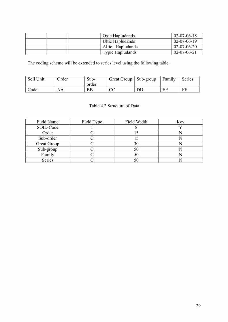
Oxic Hapludands 02-07-06-18Ultic Hapludands 02-07-06-19Alfic Hapludands 02-07-06-20Typic Hapludands 02-07-06-21

The coding scheme will be extended to series level using the following table.

Soil Unit Order Sub-order

Great Group Sub-group Family Series

Code AA BB CC DD EE FF

Table 4.2 Structure of Data

Field Name Field Type Field Width KeySOIL-Code I 8 Y

Order C 15 NSub-order C 15 N

Great Group C 30 NSub-group C 50 N

Family C 50 NSeries C 50 N

30

5. GEOLOGY - LITHOLOGY


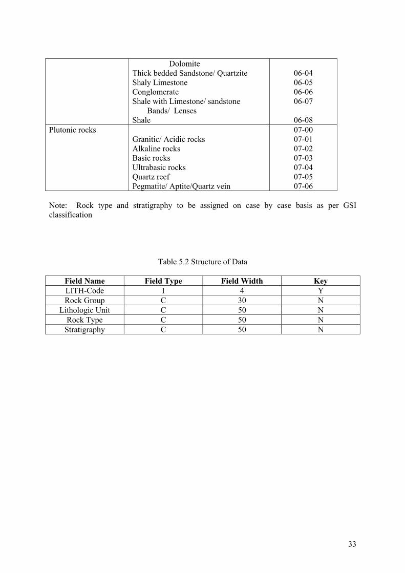
The standard classification scheme for lithology unit and rock type ( and code) is shown inTable 5.1 while the structure of data is described in Table 5.2. Only those units present in themap area will be classified, and any other unit present in the area and not covered by thescheme will be mapped and provided appropriate code.

5.2 Input Data

- Geocoded IRS LISS III FCC imagery in 1:50000 scale of summer season (withminimum vegetation cover); where necessary Kharif or Rabi season data will beadditionally used

- Existing geological and hydrogeological maps and literature

5.3 Methodology

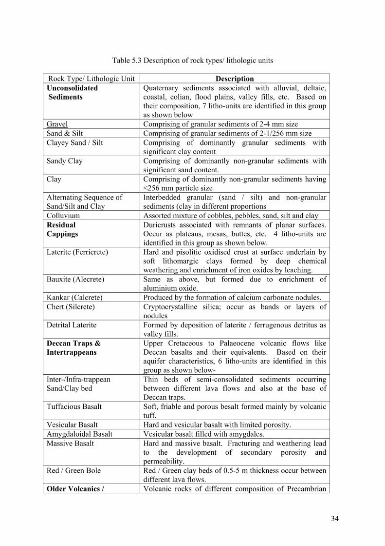
Classification and mapping of lithologic units/rock types is performed through visualinterpretation of image characteristics and terrain information, supported by the a prioriknowledge of general geologic setting of the area. The description of rock types / lithologicunits is provided in Table 5.3.

The tone (colour) and landform characteristics, and relative erodibility, drainage, soil type,land use/cover and other contextual information are used in classification. Acidic andarenaceous rocks are lighter in tone compared to basic/ argillaceous rocks. Coarse grainedrocks with higher porosity and permeability appear brighter as compared to fine grainedrocks with higher moisture retaining capacity. Highly resistant rock formations occur asdifferent hill types depending on their texture and internal structure, while the easily erodiblerocks occur as different types of plains and valleys. Dentritic drainage indicateshomogeneous rocks, while trellis, rectangular and parallel drainage patterns indicatestructural and lithologic controls. Coarse drainage texture indicates highly porous andpermeable rock formations, while fine drainage texture is present in less pervious formations.Coarse textured and light coloured soils indicate acidic/ arenaceous rocks rich in quartz andfeldspars, while fine textured and dark coloured soils indicate basic/ argillaceous rocks.Convergence of evidence from different interpretation elements will be followed for reliableclassification. The contacts of identified rock types will be extended over large areas basedon tonal contrast or landform on satellite imagery. Inferred boundaries (where the contrast isnot adequate) is marked by different symbol. The rock types are mapped and labeled as perclassification scheme (Table 5.1).

After preliminary interpretation field visit is conducted for proper identification andclassification of rock types.


31

The classified map will be scanned and digitized using an appropriate scanner (Annexure 2).The Arc/Info coverage will be created and edited to remove digitization errors, and thetopology will be built. The features will be labeled as per codes/symbols defined in Table 5.1and 5.2.. The coverage will then be projected and transformed into polyconic projection andcoordinate system in meters. The transformation process will involve geometric rectificationthrough Ground Control Points (GCPs) identified on the input coverage and correspondingSOI map. The HP data specification standards in Table 2.2 need to be conformed. Theresulting GIS coverage will be backed up in CD and labeled with corresponding SOI mapsheet number, theme, generating agency, and generation date.


5.4 Output Products


32

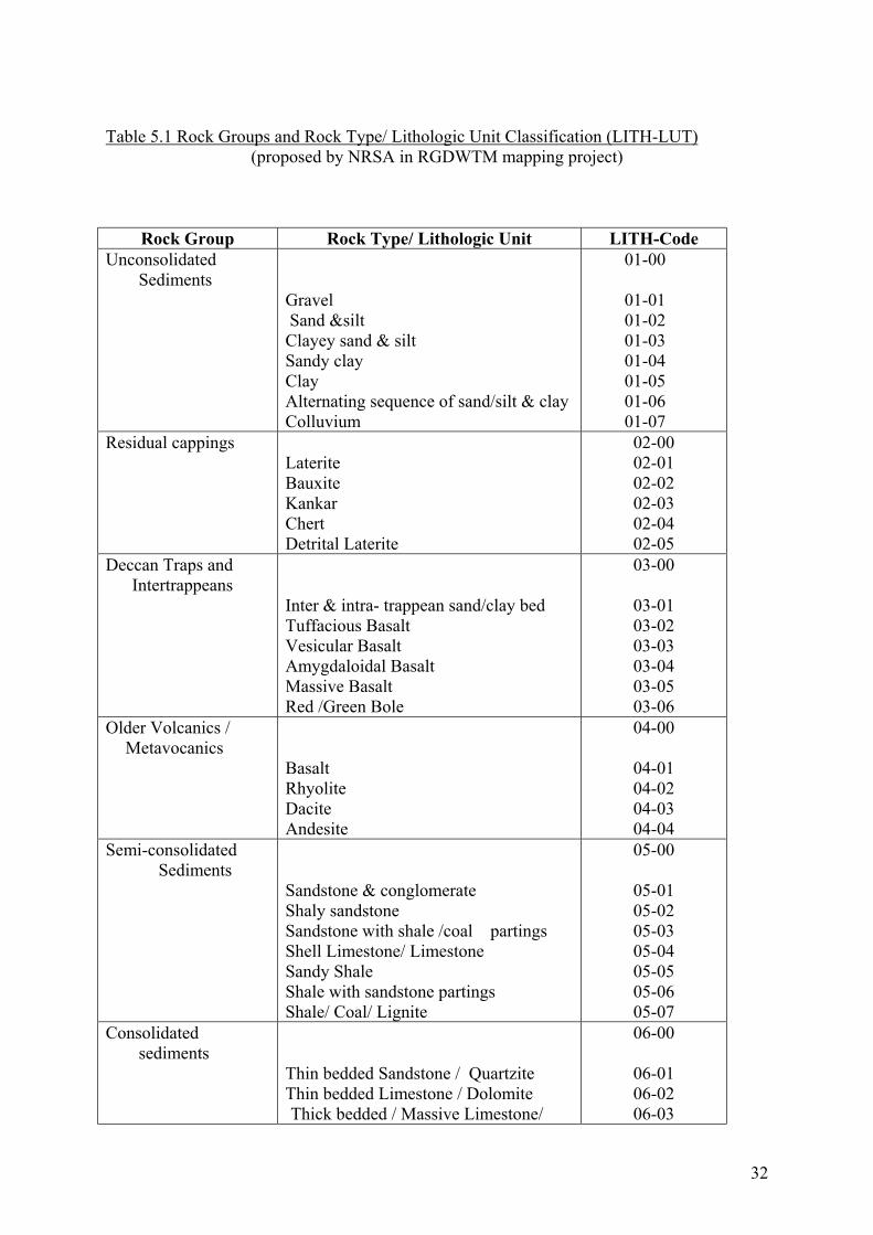
Table 5.1 Rock Groups and Rock Type/ Lithologic Unit Classification (LITH-LUT)(proposed by NRSA in RGDWTM mapping project)

Rock Group Rock Type/ Lithologic Unit LITH-CodeUnconsolidated

SedimentsGravel Sand &siltClayey sand & siltSandy clayClayAlternating sequence of sand/silt & clayColluvium

01-00

01-01 01-02 01-03 01-04 01-05 01-06 01-07

Residual cappingsLateriteBauxiteKankarChertDetrital Laterite

02-0002-0102-0202-0302-0402-05

Deccan Traps andIntertrappeans

Inter & intra- trappean sand/clay bedTuffacious BasaltVesicular BasaltAmygdaloidal BasaltMassive BasaltRed /Green Bole

03-00

03-0103-0203-0303-0403-0503-06

Older Volcanics /Metavocanics

BasaltRhyoliteDaciteAndesite

04-00

04-0104-0204-0304-04

Semi-consolidatedSediments

Sandstone & conglomerateShaly sandstoneSandstone with shale /coal partingsShell Limestone/ LimestoneSandy ShaleShale with sandstone partingsShale/ Coal/ Lignite

05-00

05-0105-0205-0305-0405-0505-0605-07

Consolidatedsediments

Thin bedded Sandstone / QuartziteThin bedded Limestone / DolomiteThick bedded / Massive Limestone/

06-00

06-0106-0206-03

33

DolomiteThick bedded Sandstone/ QuartziteShaly LimestoneConglomerateShale with Limestone/ sandstone

Bands/ LensesShale

06-0406-0506-0606-07

06-08Plutonic rocks

Granitic/ Acidic rocksAlkaline rocksBasic rocksUltrabasic rocksQuartz reefPegmatite/ Aptite/Quartz vein

07-0007-0107-0207-0307-0407-0507-06

Note: Rock type and stratigraphy to be assigned on case by case basis as per GSIclassification


Field Name Field Type Field Width KeyLITH-Code I 4 YRock Group C 30 N

Lithologic Unit C 50 NRock Type C 50 N

Stratigraphy C 50 N

34

Table 5.3 Description of rock types/ lithologic units

Rock Type/ Lithologic Unit DescriptionUnconsolidated Sediments

Quaternary sediments associated with alluvial, deltaic,coastal, eolian, flood plains, valley fills, etc. Based ontheir composition, 7 litho-units are identified in this groupas shown below

Gravel Comprising of granular sediments of 2-4 mm sizeSand & Silt Comprising of granular sediments of 2-1/256 mm sizeClayey Sand / Silt Comprising of dominantly granular sediments with

significant clay contentSandy Clay Comprising of dominantly non-granular sediments with

significant sand content.Clay Comprising of dominantly non-granular sediments having

<256 mm particle sizeAlternating Sequence ofSand/Silt and Clay

Interbedded granular (sand / silt) and non-granularsediments (clay in different proportions

Colluvium Assorted mixture of cobbles, pebbles, sand, silt and clayResidualCappings

Duricrusts associated with remnants of planar surfaces.Occur as plateaus, mesas, buttes, etc. 4 litho-units areidentified in this group as shown below.

Laterite (Ferricrete) Hard and pisolitic oxidised crust at surface underlain bysoft lithomargic clays formed by deep chemicalweathering and enrichment of iron oxides by leaching.

Bauxite (Alecrete) Same as above, but formed due to enrichment ofaluminium oxide.

Kankar (Calcrete) Produced by the formation of calcium carbonate nodules.Chert (Silcrete) Cryptocrystalline silica; occur as bands or layers of

nodulesDetrital Laterite Formed by deposition of laterite / ferrugenous detritus as

valley fills.Deccan Traps &Intertrappeans

Upper Cretaceous to Palaeocene volcanic flows likeDeccan basalts and their equivalents. Based on theiraquifer characteristics, 6 litho-units are identified in thisgroup as shown below-

Inter-/Infra-trappeanSand/Clay bed

Thin beds of semi-consolidated sediments occurringbetween different lava flows and also at the base ofDeccan traps.

Tuffacious Basalt Soft, friable and porous besalt formed mainly by volcanictuff.

Vesicular Basalt Hard and vesicular basalt with limited porosity.Amygdaloidal Basalt Vesicular basalt filled with amygdales.Massive Basalt Hard and massive basalt. Fracturing and weathering lead

to the development of secondary porosity andpermeability.

Red / Green Bole Red / Green clay beds of 0.5-5 m thickness occur betweendifferent lava flows.

Older Volcanics / Volcanic rocks of different composition of Precambrian

35

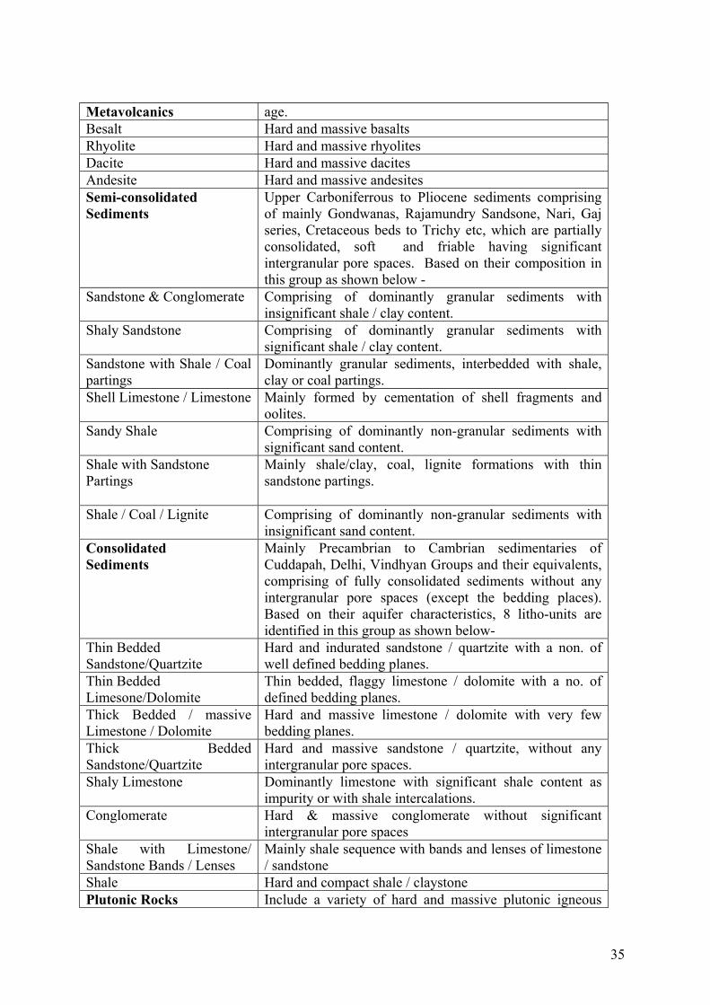
Metavolcanics age.Besalt Hard and massive basaltsRhyolite Hard and massive rhyolitesDacite Hard and massive dacitesAndesite Hard and massive andesitesSemi-consolidatedSediments

Upper Carboniferrous to Pliocene sediments comprisingof mainly Gondwanas, Rajamundry Sandsone, Nari, Gajseries, Cretaceous beds to Trichy etc, which are partiallyconsolidated, soft and friable having significantintergranular pore spaces. Based on their composition inthis group as shown below -

Sandstone & Conglomerate Comprising of dominantly granular sediments withinsignificant shale / clay content.

Shaly Sandstone Comprising of dominantly granular sediments withsignificant shale / clay content.

Sandstone with Shale / Coalpartings

Dominantly granular sediments, interbedded with shale,clay or coal partings.

Shell Limestone / Limestone Mainly formed by cementation of shell fragments andoolites.

Sandy Shale Comprising of dominantly non-granular sediments withsignificant sand content.

Shale with SandstonePartings

Mainly shale/clay, coal, lignite formations with thinsandstone partings.

Shale / Coal / Lignite Comprising of dominantly non-granular sediments withinsignificant sand content.

ConsolidatedSediments

Mainly Precambrian to Cambrian sedimentaries ofCuddapah, Delhi, Vindhyan Groups and their equivalents,comprising of fully consolidated sediments without anyintergranular pore spaces (except the bedding places).Based on their aquifer characteristics, 8 litho-units areidentified in this group as shown below-

Thin BeddedSandstone/Quartzite

Hard and indurated sandstone / quartzite with a non. ofwell defined bedding planes.

Thin BeddedLimesone/Dolomite

Thin bedded, flaggy limestone / dolomite with a no. ofdefined bedding planes.

Thick Bedded / massiveLimestone / Dolomite

Hard and massive limestone / dolomite with very fewbedding planes.

Thick BeddedSandstone/Quartzite

Hard and massive sandstone / quartzite, without anyintergranular pore spaces.

Shaly Limestone Dominantly limestone with significant shale content asimpurity or with shale intercalations.

Conglomerate Hard & massive conglomerate without significantintergranular pore spaces

Shale with Limestone/Sandstone Bands / Lenses

Mainly shale sequence with bands and lenses of limestone/ sandstone

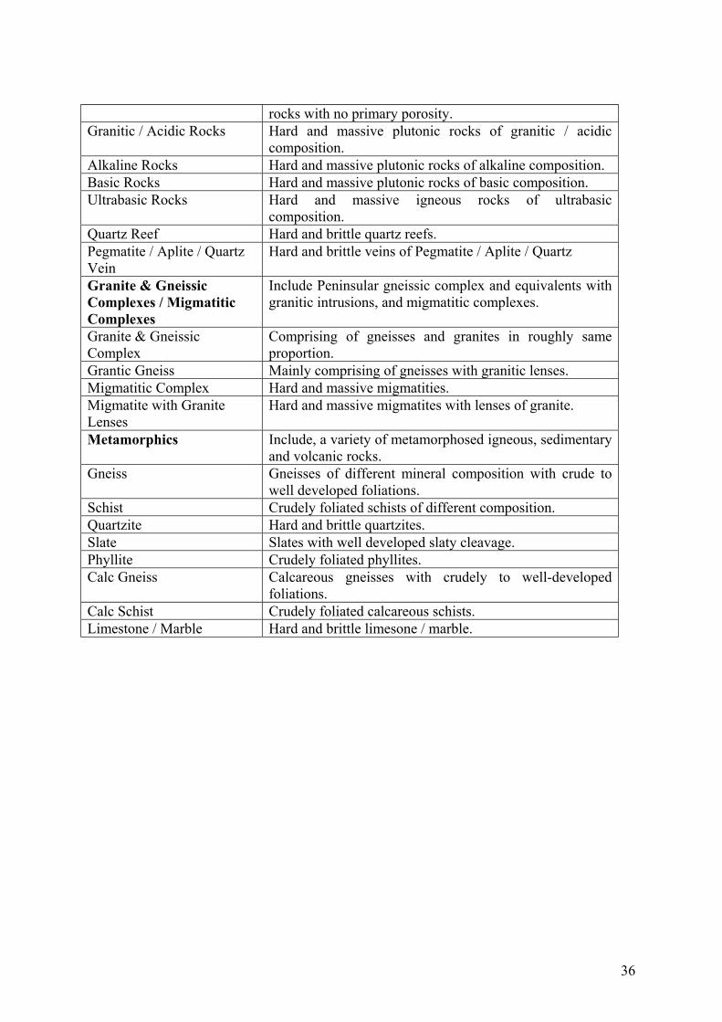
Shale Hard and compact shale / claystonePlutonic Rocks Include a variety of hard and massive plutonic igneous

36

rocks with no primary porosity.Granitic / Acidic Rocks Hard and massive plutonic rocks of granitic / acidic

composition.Alkaline Rocks Hard and massive plutonic rocks of alkaline composition.Basic Rocks Hard and massive plutonic rocks of basic composition.Ultrabasic Rocks Hard and massive igneous rocks of ultrabasic

composition.Quartz Reef Hard and brittle quartz reefs.Pegmatite / Aplite / QuartzVein

Hard and brittle veins of Pegmatite / Aplite / Quartz

Granite & GneissicComplexes / MigmatiticComplexes

Include Peninsular gneissic complex and equivalents withgranitic intrusions, and migmatitic complexes.

Granite & GneissicComplex

Comprising of gneisses and granites in roughly sameproportion.

Grantic Gneiss Mainly comprising of gneisses with granitic lenses.Migmatitic Complex Hard and massive migmatities.Migmatite with GraniteLenses

Hard and massive migmatites with lenses of granite.

Metamorphics Include, a variety of metamorphosed igneous, sedimentaryand volcanic rocks.

Gneiss Gneisses of different mineral composition with crude towell developed foliations.

Schist Crudely foliated schists of different composition.Quartzite Hard and brittle quartzites.Slate Slates with well developed slaty cleavage.Phyllite Crudely foliated phyllites.Calc Gneiss Calcareous gneisses with crudely to well-developed

foliations.Calc Schist Crudely foliated calcareous schists.Limestone / Marble Hard and brittle limesone / marble.

37

6. GEOLOGY – STRUCTURES


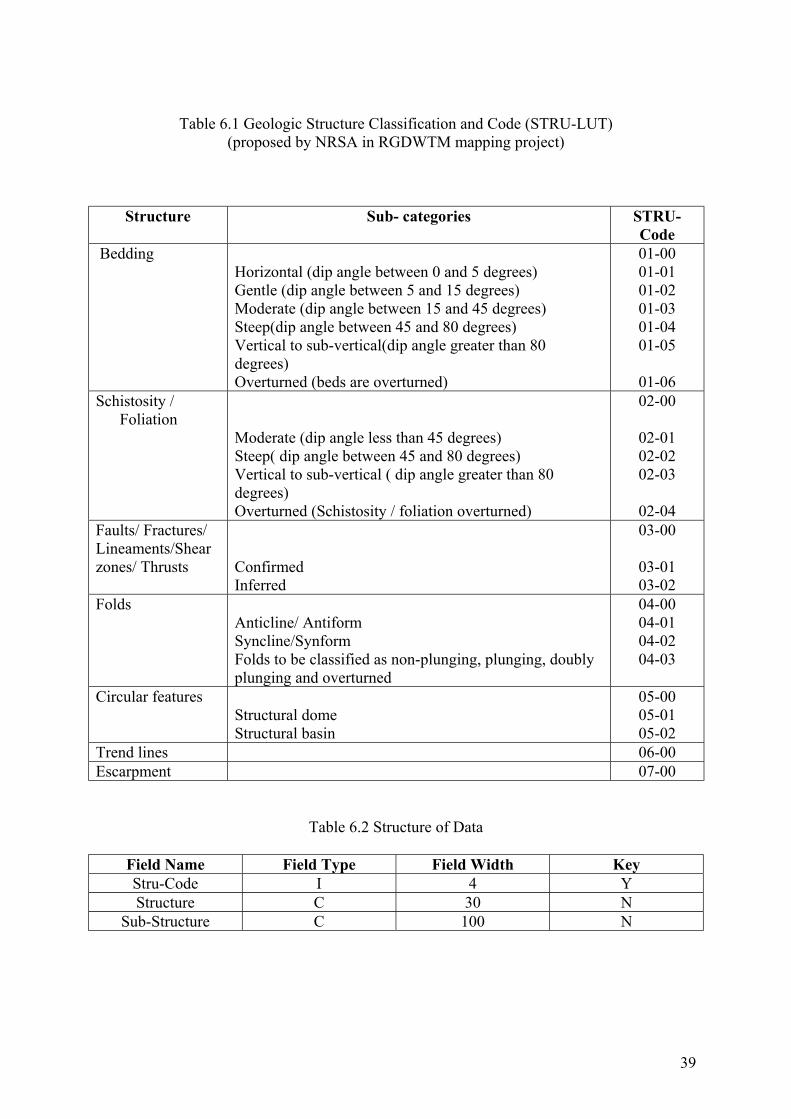
The geological structures will be mapped as per the classification scheme in Table 6.1. Onlythose units present in the map area will be classified, and any other unit present in the areaand not covered by the scheme will be mapped and provided appropriate code.

6.2 Input Data



6.3 Methodology

Different types of primary and secondary geological structures (attitude of beds, schisticity /foliation, folds, lineaments, circular features, etc..) can be visually interpreted by studying thelandforms, slope asymmetry, outcrop pattern, drainage pattern, and stream/ river courses.Lineaments (faults, fractures, shear zones, and thrusts.) appear as linear and curvilinear lineson the satellite imagery, and are often indicated by the presence of moisture, alignment ofvegetation, straight drainage courses, alignment of tanks / ponds,etc.. Lineaments are furthersub-divided based on image characteristics and geological evidence.

The attitude of beds (strike and dip) are estimated by studying the slope asymmetry,landform, drainage characteristics, etc.. For instance horizontal to sub-horizontal beds showmesa / butte type of landform, dentritic drainage pattern and tonal / colour banding parallel tothe contour lines; inclined beds show triangular dip facets, cuestas, homoclines and hogbacks.The Schistosity / foliation of the rocks are shown as numerous thin, wavy and discontinuoustrend lines. Non-plunging and plunging folds are mapped from the marker horizons. Non-plunging folds produce outcropping in parallel belts, and plunging folds produce V or Ushaped outcrop pattern. Doubly plunging folds are indicated by oval shaped outcrops.Further classification into anticline or syncline can be made on the basis of dip direction ofbeds. Circular features, representing structural domes/ basins, sub-surface igneous intrusions,salt domes, etc. show circular to quasi-circular outcrops and trend lines with radial/ annulardrainage pattern. Reference to existing literature can support confirmation of interpreteddetails. The geological structures will be mapped with standard symbols.

The pre-field structural map will be checked in the field and validated.


The classified map will be scanned and digitized using an appropriate scanner (Annexure 2).The Arc/Info coverage will be created and edited to remove digitization errors, and thetopology will be built. The features will be labeled as per codes/symbols defined in Table 6.1

38

and 6.2.. The coverage will then be projected and transformed into polyconic projection andcoordinate system in meters. The transformation process will involve geometric rectificationthrough Ground Control Points (GCPs) identified on the input coverage and correspondingSOI map. The HP data specification standards in Table 2.2 need to be conformed. Theresulting GIS coverage will be backed up in CD and labeled with corresponding SOI mapsheet number, theme, generating agency, and generation date.


6.4 Output Products


39

Table 6.1 Geologic Structure Classification and Code (STRU-LUT)(proposed by NRSA in RGDWTM mapping project)

Structure Sub- categories STRU-Code

BeddingHorizontal (dip angle between 0 and 5 degrees)Gentle (dip angle between 5 and 15 degrees)Moderate (dip angle between 15 and 45 degrees)Steep(dip angle between 45 and 80 degrees)Vertical to sub-vertical(dip angle greater than 80degrees)Overturned (beds are overturned)

01-0001-0101-0201-0301-0401-05

01-06Schistosity /

FoliationModerate (dip angle less than 45 degrees)Steep( dip angle between 45 and 80 degrees)Vertical to sub-vertical ( dip angle greater than 80degrees)Overturned (Schistosity / foliation overturned)

02-00

02-0102-0202-03

02-04Faults/ Fractures/Lineaments/Shearzones/ Thrusts Confirmed

Inferred

03-00

03-0103-02

FoldsAnticline/ AntiformSyncline/SynformFolds to be classified as non-plunging, plunging, doublyplunging and overturned

04-0004-0104-0204-03

Circular featuresStructural domeStructural basin

05-0005-0105-02

Trend lines 06-00Escarpment 07-00


Field Name Field Type Field Width KeyStru-Code I 4 YStructure C 30 N

Sub-Structure C 100 N

40

7. GEOMORPHOLOGY


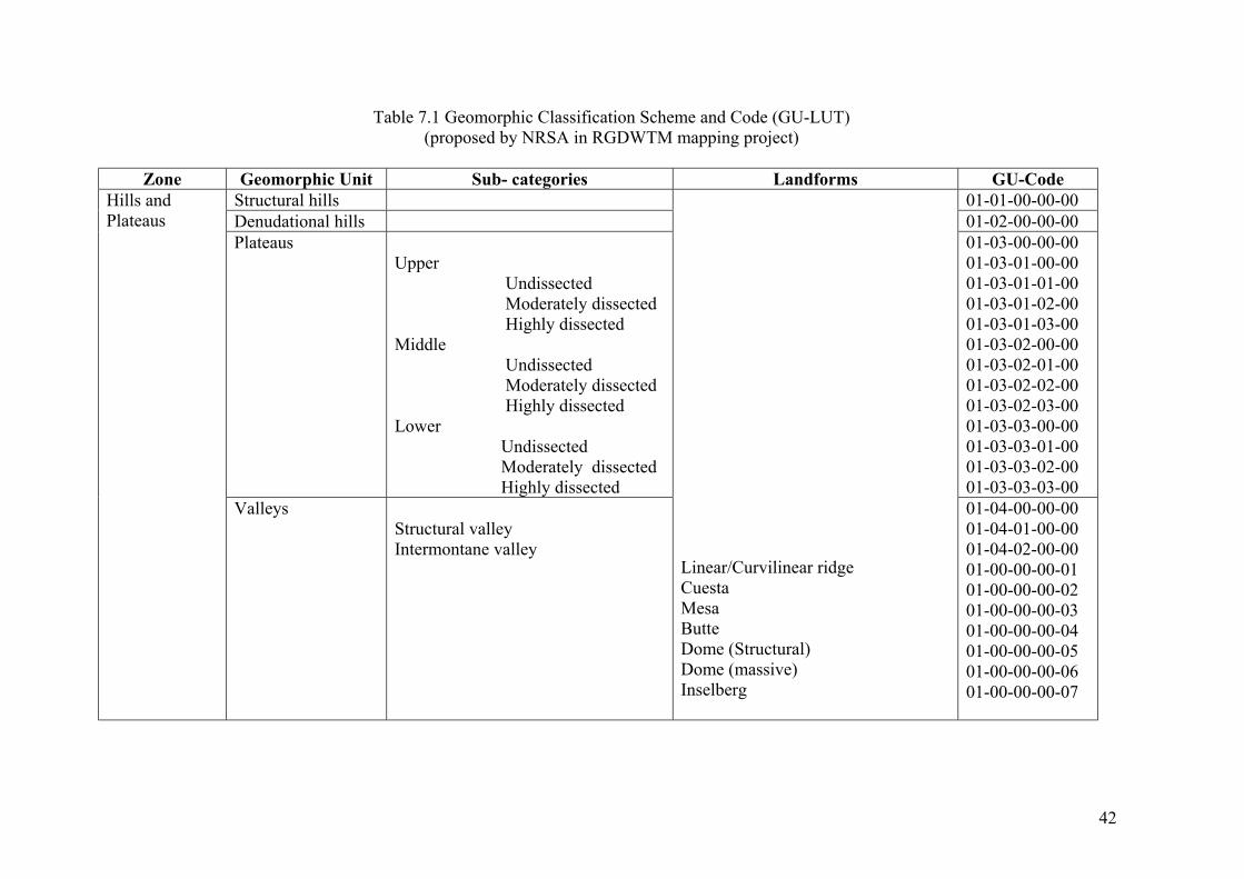
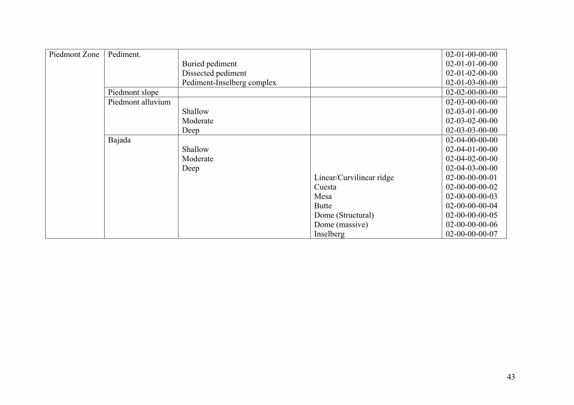
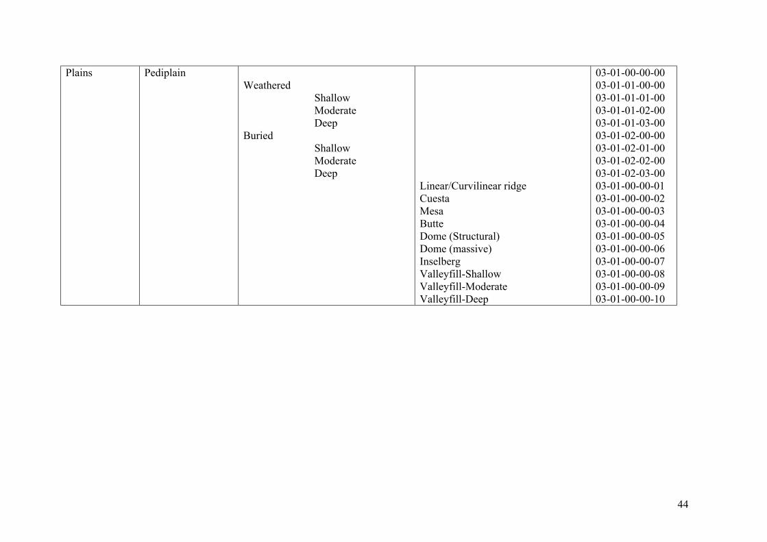
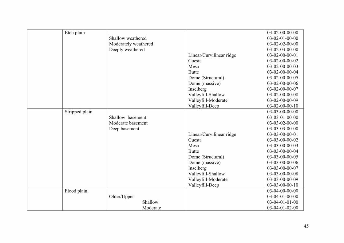
Geomorphic units/ different landforms will be mapped as per the classification scheme (andcode) in Table 7.1, and the structure of data is described in Table 7.2. While the scheme iscomprehensive only those units present in the area to be mapped will be classified, and anyother unit present in the area and not listed in Table 7.1 will be classified and appropriatecode/ symbol used.

7.2 Input Data



7.3 Methodology

The geomorphic units/ landforms in the classification scheme are described in Table 7.3. Thesatellite imagery will be visually interpreted into geomorphic units/ landforms based onimage elements such as tone, texture, shape, size, location and association, physiography,genesis of landforms, nature of rocks/ sediments, and associated geological structures. Thetopographic information in SOI topomaps aids in interpreting satellite imagery. Three majorgeomorphic units – hills and plateaus, piedmont zones, and plains- based on physiographyand relief. Within each zone different geomorphic units will be mapped based on landformcharacteristics, their areal extent, depth of weathering, thickness of deposition, etc.

The interpreted geomorphic units/landforms will be verified through field visits, in which thedepth of weathering, nature of weathered material, thickness of deposition, nature ofdeposited material, etc. are examined at nala and stream cuttings, existing wells, lithologs ofwells drilled, etc..


The classified map will be scanned and digitized using an appropriate scanner (Annexure 2).The Arc/Info coverage will be created and edited to remove digitization errors, and thetopology will be built. The features will be labeled as per codes/symbols defined in Table 7.1and 7.2. The coverage will then be projected and transformed into polyconic projection andcoordinate system in meters. The transformation process will involve geometric rectificationthrough Ground Control Points (GCPs) identified on the input coverage and correspondingSOI map. The HP data specification standards in Table 2.2 need to be conformed. Theresulting GIS coverage will be backed up in CD and labeled with corresponding SOI mapsheet number, theme, generating agency, and generation date.


41

6.4 Output Products


42

Table 7.1 Geomorphic Classification Scheme and Code (GU-LUT)(proposed by NRSA in RGDWTM mapping project)

Zone Geomorphic Unit Sub- categories Landforms GU-CodeStructural hills 01-01-00-00-00Denudational hills 01-02-00-00-00Plateaus

Upper Undissected Moderately dissected Highly dissectedMiddle Undissected Moderately dissected Highly dissectedLower Undissected Moderately dissected Highly dissected

01-03-00-00-0001-03-01-00-0001-03-01-01-0001-03-01-02-0001-03-01-03-0001-03-02-00-0001-03-02-01-0001-03-02-02-0001-03-02-03-0001-03-03-00-0001-03-03-01-0001-03-03-02-0001-03-03-03-00

Hills andPlateaus

ValleysStructural valleyIntermontane valley

Linear/Curvilinear ridgeCuestaMesaButteDome (Structural)Dome (massive)Inselberg

01-04-00-00-0001-04-01-00-0001-04-02-00-0001-00-00-00-0101-00-00-00-0201-00-00-00-0301-00-00-00-0401-00-00-00-0501-00-00-00-0601-00-00-00-07

43

Pediment.Buried pedimentDissected pedimentPediment-Inselberg complex

02-01-00-00-0002-01-01-00-0002-01-02-00-0002-01-03-00-00

Piedmont slope 02-02-00-00-00Piedmont alluvium

ShallowModerateDeep

02-03-00-00-0002-03-01-00-0002-03-02-00-0002-03-03-00-00

Piedmont Zone

BajadaShallowModerateDeep

Linear/Curvilinear ridgeCuestaMesaButteDome (Structural)Dome (massive)Inselberg

02-04-00-00-0002-04-01-00-0002-04-02-00-0002-04-03-00-0002-00-00-00-0102-00-00-00-0202-00-00-00-0302-00-00-00-0402-00-00-00-0502-00-00-00-0602-00-00-00-07

44

Plains PediplainWeathered Shallow Moderate DeepBuried Shallow Moderate Deep

Linear/Curvilinear ridgeCuestaMesaButteDome (Structural)Dome (massive)InselbergValleyfill-ShallowValleyfill-ModerateValleyfill-Deep

03-01-00-00-0003-01-01-00-0003-01-01-01-0003-01-01-02-0003-01-01-03-0003-01-02-00-0003-01-02-01-0003-01-02-02-0003-01-02-03-0003-01-00-00-0103-01-00-00-0203-01-00-00-0303-01-00-00-0403-01-00-00-0503-01-00-00-0603-01-00-00-0703-01-00-00-0803-01-00-00-0903-01-00-00-10

45

Etch plainShallow weatheredModerately weatheredDeeply weathered


03-02-00-00-0003-02-01-00-0003-02-02-00-0003-02-03-00-0003-02-00-00-0103-02-00-00-0203-02-00-00-0303-02-00-00-0403-02-00-00-0503-02-00-00-0603-02-00-00-0703-02-00-00-0803-02-00-00-0903-02-00-00-10

Stripped plainShallow basementModerate basementDeep basement


03-03-00-00-0003-03-01-00-0003-03-02-00-0003-03-03-00-0003-03-00-00-0103-03-00-00-0203-03-00-00-0303-03-00-00-0403-03-00-00-0503-03-00-00-0603-03-00-00-0703-03-00-00-0803-03-00-00-0903-03-00-00-10

Flood plainOlder/Upper Shallow Moderate

03-04-00-00-0003-04-01-00-0003-04-01-01-0003-04-01-02-00

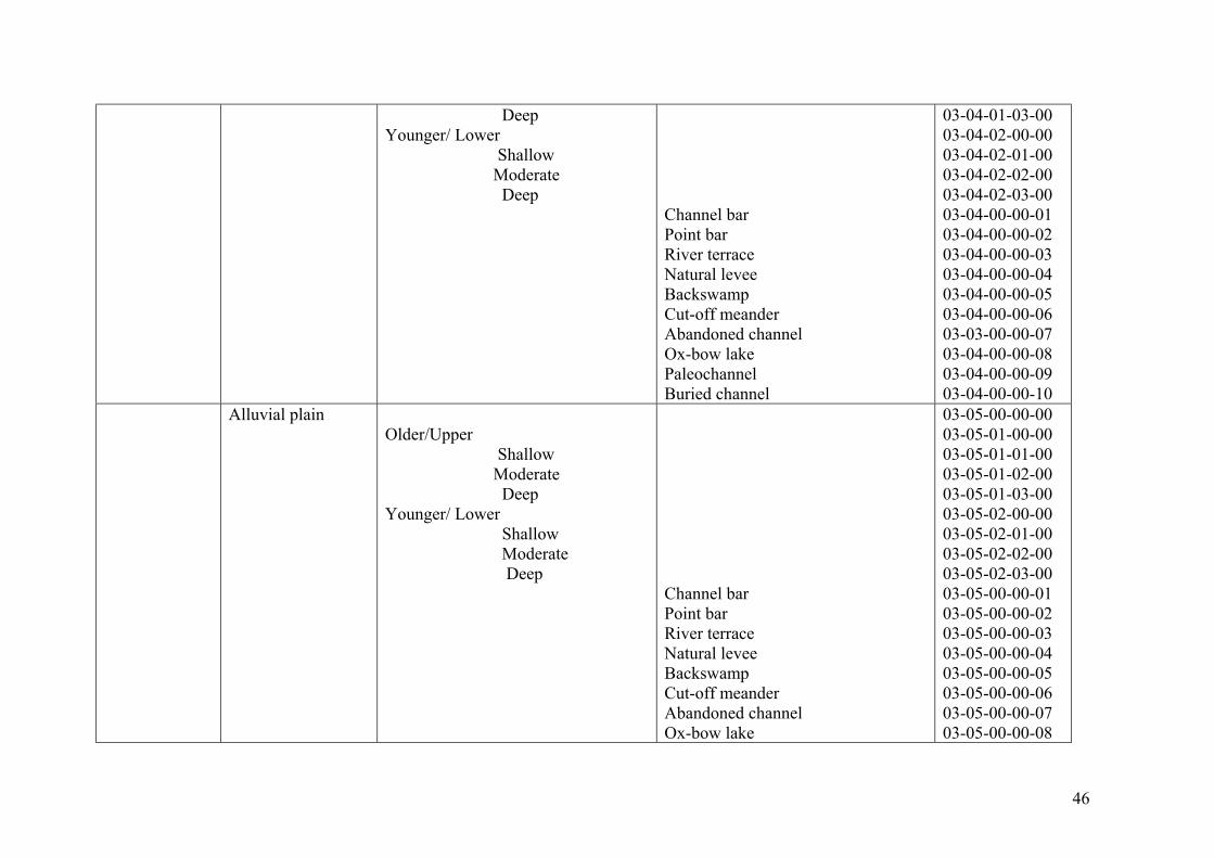
46

DeepYounger/ Lower Shallow Moderate Deep

Channel barPoint barRiver terraceNatural leveeBackswampCut-off meanderAbandoned channelOx-bow lakePaleochannelBuried channel

03-04-01-03-0003-04-02-00-0003-04-02-01-0003-04-02-02-0003-04-02-03-0003-04-00-00-0103-04-00-00-0203-04-00-00-0303-04-00-00-0403-04-00-00-0503-04-00-00-0603-03-00-00-0703-04-00-00-0803-04-00-00-0903-04-00-00-10

Alluvial plainOlder/Upper Shallow Moderate DeepYounger/ Lower Shallow Moderate Deep

Channel barPoint barRiver terraceNatural leveeBackswampCut-off meanderAbandoned channelOx-bow lake

03-05-00-00-0003-05-01-00-0003-05-01-01-0003-05-01-02-0003-05-01-03-0003-05-02-00-0003-05-02-01-0003-05-02-02-0003-05-02-03-0003-05-00-00-0103-05-00-00-0203-05-00-00-0303-05-00-00-0403-05-00-00-0503-05-00-00-0603-05-00-00-0703-05-00-00-08

47

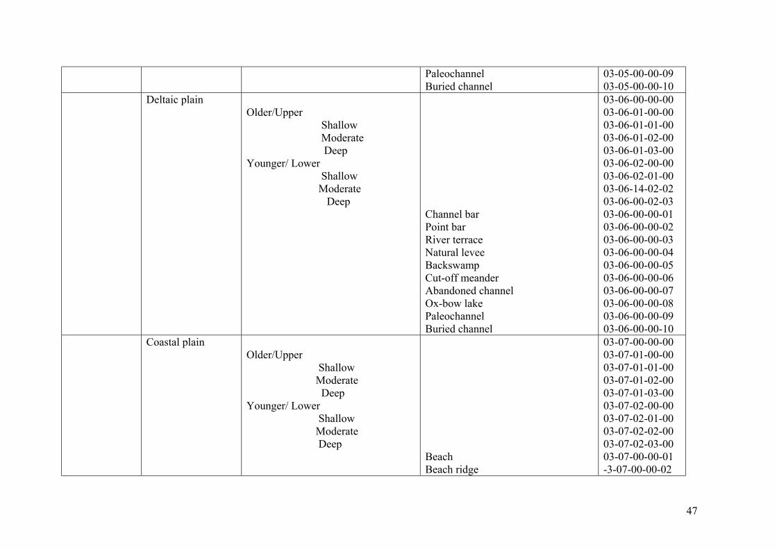
PaleochannelBuried channel

03-05-00-00-0903-05-00-00-10

Deltaic plainOlder/Upper Shallow Moderate DeepYounger/ Lower Shallow Moderate Deep

Channel barPoint barRiver terraceNatural leveeBackswampCut-off meanderAbandoned channelOx-bow lakePaleochannelBuried channel

03-06-00-00-0003-06-01-00-0003-06-01-01-0003-06-01-02-0003-06-01-03-0003-06-02-00-0003-06-02-01-0003-06-14-02-0203-06-00-02-0303-06-00-00-0103-06-00-00-0203-06-00-00-0303-06-00-00-0403-06-00-00-0503-06-00-00-0603-06-00-00-0703-06-00-00-0803-06-00-00-0903-06-00-00-10

Coastal plainOlder/Upper Shallow Moderate DeepYounger/ Lower Shallow Moderate Deep

BeachBeach ridge

03-07-00-00-0003-07-01-00-0003-07-01-01-0003-07-01-02-0003-07-01-03-0003-07-02-00-0003-07-02-01-0003-07-02-02-0003-07-02-03-0003-07-00-00-01-3-07-00-00-02

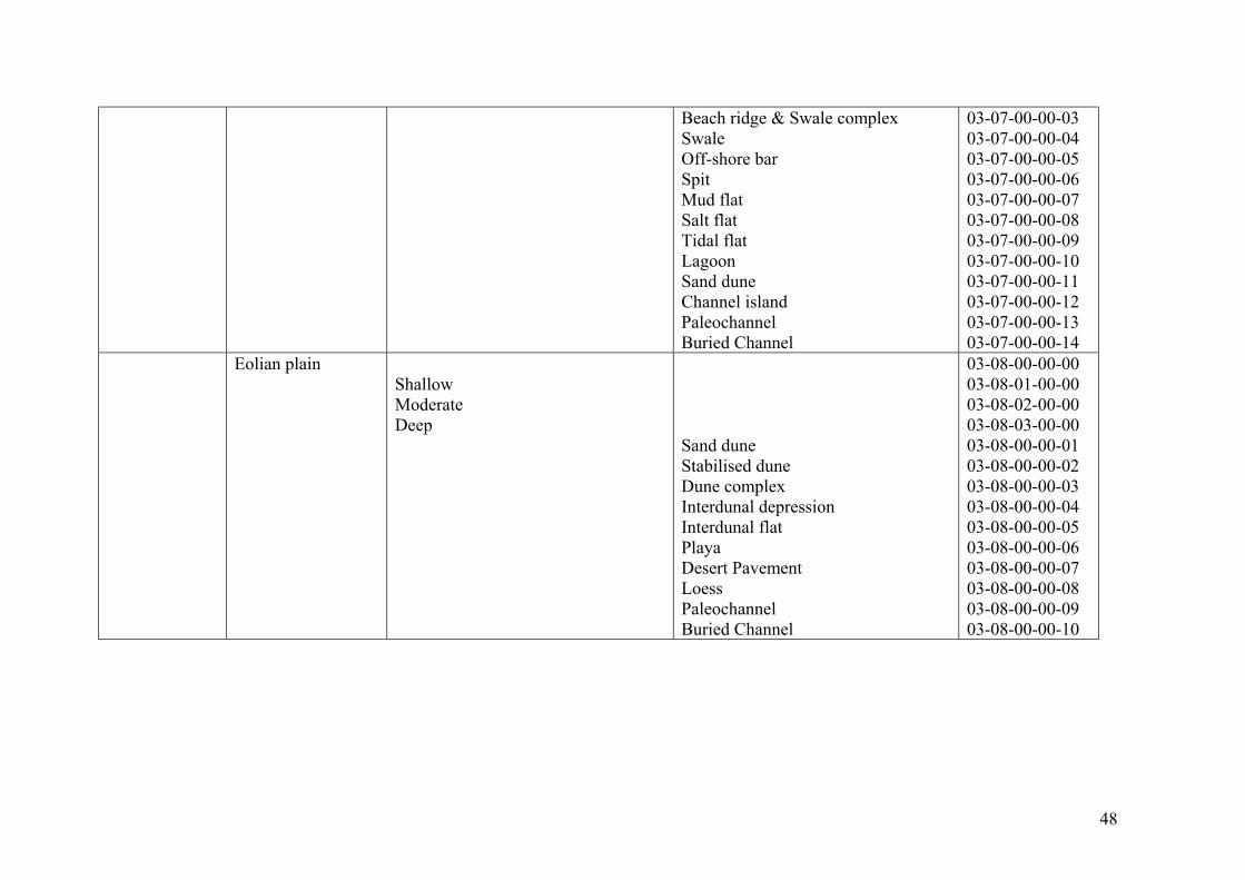
48

Beach ridge & Swale complexSwaleOff-shore barSpitMud flatSalt flatTidal flatLagoonSand duneChannel islandPaleochannelBuried Channel

03-07-00-00-0303-07-00-00-0403-07-00-00-0503-07-00-00-0603-07-00-00-0703-07-00-00-0803-07-00-00-0903-07-00-00-1003-07-00-00-1103-07-00-00-1203-07-00-00-1303-07-00-00-14

Eolian plainShallowModerateDeep

Sand duneStabilised duneDune complexInterdunal depressionInterdunal flatPlayaDesert PavementLoessPaleochannelBuried Channel

03-08-00-00-0003-08-01-00-0003-08-02-00-0003-08-03-00-0003-08-00-00-0103-08-00-00-0203-08-00-00-0303-08-00-00-0403-08-00-00-0503-08-00-00-0603-08-00-00-0703-08-00-00-0803-08-00-00-0903-08-00-00-10

49

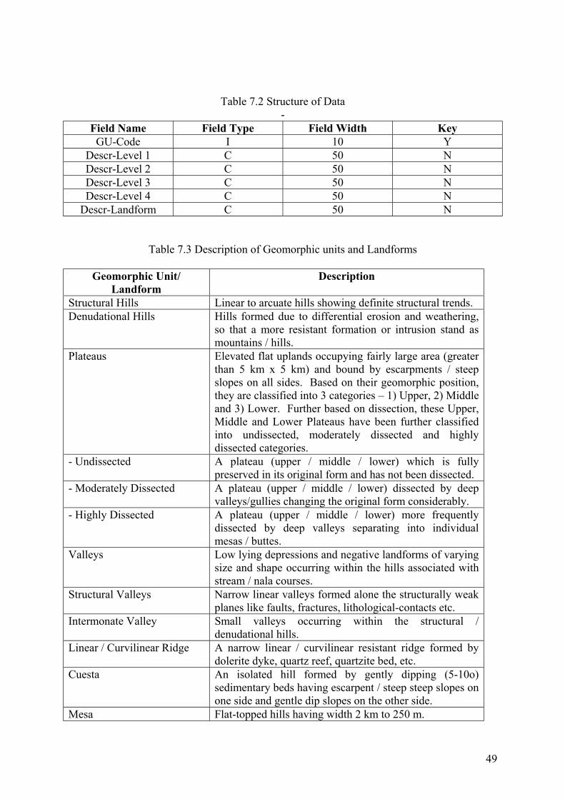
Table 7.2 Structure of Data-

Field Name Field Type Field Width KeyGU-Code I 10 Y

Descr-Level 1 C 50 NDescr-Level 2 C 50 NDescr-Level 3 C 50 NDescr-Level 4 C 50 N

Descr-Landform C 50 N

Table 7.3 Description of Geomorphic units and Landforms

Geomorphic Unit/Landform

Description

Structural Hills Linear to arcuate hills showing definite structural trends.Denudational Hills Hills formed due to differential erosion and weathering,

so that a more resistant formation or intrusion stand asmountains / hills.

Plateaus Elevated flat uplands occupying fairly large area (greaterthan 5 km x 5 km) and bound by escarpments / steepslopes on all sides. Based on their geomorphic position,they are classified into 3 categories – 1) Upper, 2) Middleand 3) Lower. Further based on dissection, these Upper,Middle and Lower Plateaus have been further classifiedinto undissected, moderately dissected and highlydissected categories.

- Undissected A plateau (upper / middle / lower) which is fullypreserved in its original form and has not been dissected.

- Moderately Dissected A plateau (upper / middle / lower) dissected by deepvalleys/gullies changing the original form considerably.

- Highly Dissected A plateau (upper / middle / lower) more frequentlydissected by deep valleys separating into individualmesas / buttes.

Valleys Low lying depressions and negative landforms of varyingsize and shape occurring within the hills associated withstream / nala courses.

Structural Valleys Narrow linear valleys formed alone the structurally weakplanes like faults, fractures, lithological-contacts etc.

Intermonate Valley Small valleys occurring within the structural /denudational hills.

Linear / Curvilinear Ridge A narrow linear / curvilinear resistant ridge formed bydolerite dyke, quartz reef, quartzite bed, etc.

Cuesta An isolated hill formed by gently dipping (5-10o)sedimentary beds having escarpent / steep steep slopes onone side and gentle dip slopes on the other side.

Mesa Flat-topped hills having width 2 km to 250 m.

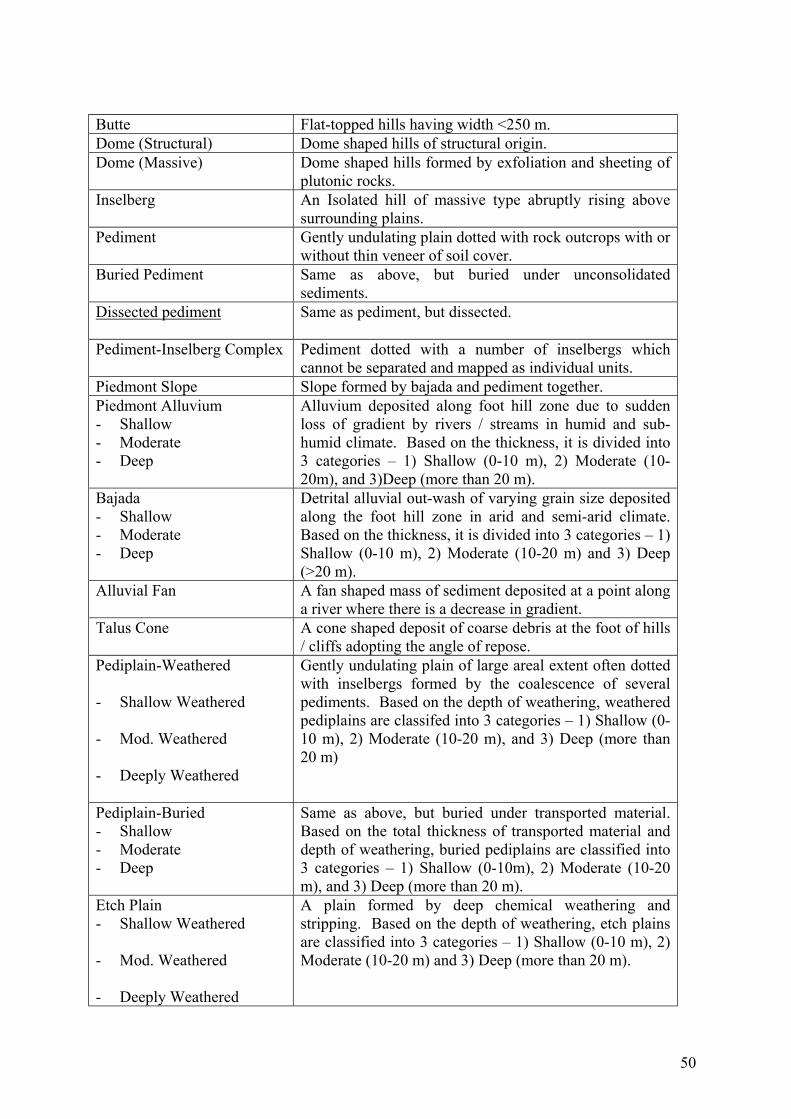
50

Butte Flat-topped hills having width <250 m.Dome (Structural) Dome shaped hills of structural origin.Dome (Massive) Dome shaped hills formed by exfoliation and sheeting of

plutonic rocks.Inselberg An Isolated hill of massive type abruptly rising above

surrounding plains.Pediment Gently undulating plain dotted with rock outcrops with or

without thin veneer of soil cover.Buried Pediment Same as above, but buried under unconsolidated

sediments.Dissected pediment Same as pediment, but dissected.

Pediment-Inselberg Complex Pediment dotted with a number of inselbergs whichcannot be separated and mapped as individual units.

Piedmont Slope Slope formed by bajada and pediment together.Piedmont Alluvium- Shallow- Moderate- Deep

Alluvium deposited along foot hill zone due to suddenloss of gradient by rivers / streams in humid and sub-humid climate. Based on the thickness, it is divided into3 categories – 1) Shallow (0-10 m), 2) Moderate (10-20m), and 3)Deep (more than 20 m).

Bajada- Shallow- Moderate- Deep

Detrital alluvial out-wash of varying grain size depositedalong the foot hill zone in arid and semi-arid climate.Based on the thickness, it is divided into 3 categories – 1)Shallow (0-10 m), 2) Moderate (10-20 m) and 3) Deep(>20 m).

Alluvial Fan A fan shaped mass of sediment deposited at a point alonga river where there is a decrease in gradient.

Talus Cone A cone shaped deposit of coarse debris at the foot of hills/ cliffs adopting the angle of repose.

Pediplain-Weathered

- Shallow Weathered

- Mod. Weathered

- Deeply Weathered

Gently undulating plain of large areal extent often dottedwith inselbergs formed by the coalescence of severalpediments. Based on the depth of weathering, weatheredpediplains are classifed into 3 categories – 1) Shallow (0-10 m), 2) Moderate (10-20 m), and 3) Deep (more than20 m)

Pediplain-Buried- Shallow- Moderate- Deep

Same as above, but buried under transported material.Based on the total thickness of transported material anddepth of weathering, buried pediplains are classified into3 categories – 1) Shallow (0-10m), 2) Moderate (10-20m), and 3) Deep (more than 20 m).

Etch Plain- Shallow Weathered

- Mod. Weathered

- Deeply Weathered

A plain formed by deep chemical weathering andstripping. Based on the depth of weathering, etch plainsare classified into 3 categories – 1) Shallow (0-10 m), 2)Moderate (10-20 m) and 3) Deep (more than 20 m).

51

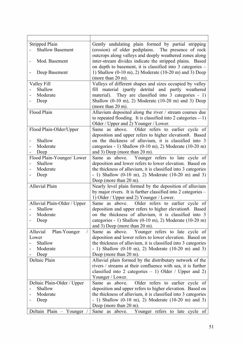
Stripped Plain- Shallow Basement

- Mod. Basement

- Deep Basement

Gently undulating plain formed by partial stripping(erosion) of older pediplains. The presence of rockoutcrops along valleys and deeply weathered zones alonginter-stream divides indicate the stripped plains. Basedon depth to basement, it is classified into 3 categories –1) Shallow (0-10 m), 2) Moderate (10-20 m) and 3) Deep(more than 20 m).

Valley Fill- Shallow- Moderate- Deep

Valleys of different shapes and sizes occupied by valleyfill material (partly detrital and partly weatheredmaterial). They are classified into 3 categories - 1)Shallow (0-10 m), 2) Moderate (10-20 m) and 3) Deep(more than 20 m).

Flood Plain Alluvium deposited along the river / stream courses dueto repeated flooding. It is classified into 2 categories -–1)Older / Upper and 2) Younger / Lower.

Flood Plain-Older/Upper

- Shallow- Moderate- Deep

Same as above. Older refers to earlier cycle ofdeposition and upper refers to higher elevation8. Basedon the thickness of alluvium, it is classified into 3categories - 1) Shallow (0-10 m), 2) Moderate (10-20 m)and 3) Deep (more than 20 m).

Flood Plain-Younger/ Lower- Shallow- Moderate- Deep

Same as above. Younger refers to late cycle ofdeposition and lower refers to lower elevation. Based onthe thickness of alluvium, it is classified into 3 categories- 1) Shallow (0-10 m), 2) Moderate (10-20 m) and 3)Deep (more than 20 m).

Alluvial Plain Nearly level plain formed by the deposition of alluviumby major rivers. It is further classified into 2 categories –1) Older / Upper and 2) Younger / Lower.

Alluvial Plain-Older / Upper- Shallow- Moderate- Deep

Same as above. Older refers to earlier cycle ofdeposition and upper refers to higher elevation8. Basedon the thickness of alluvium, it is classified into 3categories - 1) Shallow (0-10 m), 2) Moderate (10-20 m)and 3) Deep (more than 20 m).

Alluvial Plan-Younger /Lower- Shallow- Moderate- Deep


Deltaic Plain Alluvial plain formed by the distributary network of therivers / streams at their confluence with sea, it is furtherclassified into 2 categories – 1) Older / Upper and 2)Younger / Lower.

Deltaic Plain-Older / Upper- Shallow- Moderate- Deep

Same as above. Older refers to earlier cycle ofdeposition and upper refers to higher elevation. Based onthe thickness of alluvium, it is classified into 3 categories- 1) Shallow (0-10 m), 2) Moderate (10-20 m) and 3)Deep (more than 20 m).

Deltain Plain – Younger / Same as above. Younger refers to late cycle of

52

Lower- Shallow- Moderate- Deep

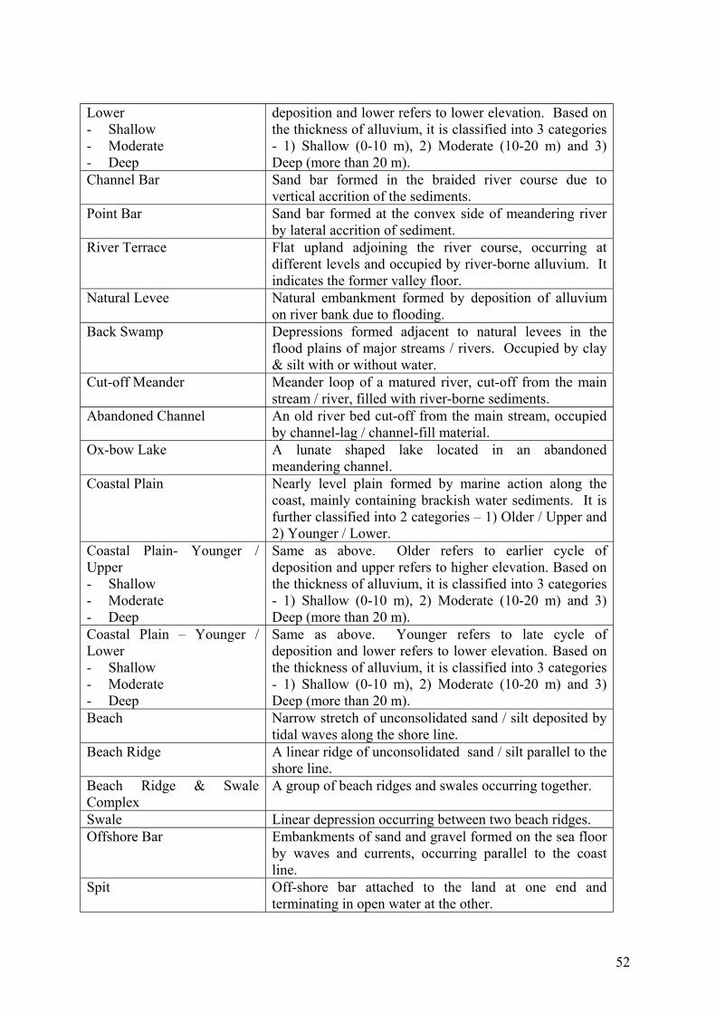
deposition and lower refers to lower elevation. Based onthe thickness of alluvium, it is classified into 3 categories- 1) Shallow (0-10 m), 2) Moderate (10-20 m) and 3)Deep (more than 20 m).

Channel Bar Sand bar formed in the braided river course due tovertical accrition of the sediments.

Point Bar Sand bar formed at the convex side of meandering riverby lateral accrition of sediment.

River Terrace Flat upland adjoining the river course, occurring atdifferent levels and occupied by river-borne alluvium. Itindicates the former valley floor.

Natural Levee Natural embankment formed by deposition of alluviumon river bank due to flooding.

Back Swamp Depressions formed adjacent to natural levees in theflood plains of major streams / rivers. Occupied by clay& silt with or without water.

Cut-off Meander Meander loop of a matured river, cut-off from the mainstream / river, filled with river-borne sediments.

Abandoned Channel An old river bed cut-off from the main stream, occupiedby channel-lag / channel-fill material.

Ox-bow Lake A lunate shaped lake located in an abandonedmeandering channel.

Coastal Plain Nearly level plain formed by marine action along thecoast, mainly containing brackish water sediments. It isfurther classified into 2 categories – 1) Older / Upper and2) Younger / Lower.

Coastal Plain- Younger /Upper- Shallow- Moderate- Deep

Same as above. Older refers to earlier cycle ofdeposition and upper refers to higher elevation. Based onthe thickness of alluvium, it is classified into 3 categories- 1) Shallow (0-10 m), 2) Moderate (10-20 m) and 3)Deep (more than 20 m).

Coastal Plain – Younger /Lower- Shallow- Moderate- Deep


Beach Narrow stretch of unconsolidated sand / silt deposited bytidal waves along the shore line.

Beach Ridge A linear ridge of unconsolidated sand / silt parallel to theshore line.

Beach Ridge & SwaleComplex

A group of beach ridges and swales occurring together.

Swale Linear depression occurring between two beach ridges.Offshore Bar Embankments of sand and gravel formed on the sea floor

by waves and currents, occurring parallel to the coastline.

Spit Off-shore bar attached to the land at one end andterminating in open water at the other.

53

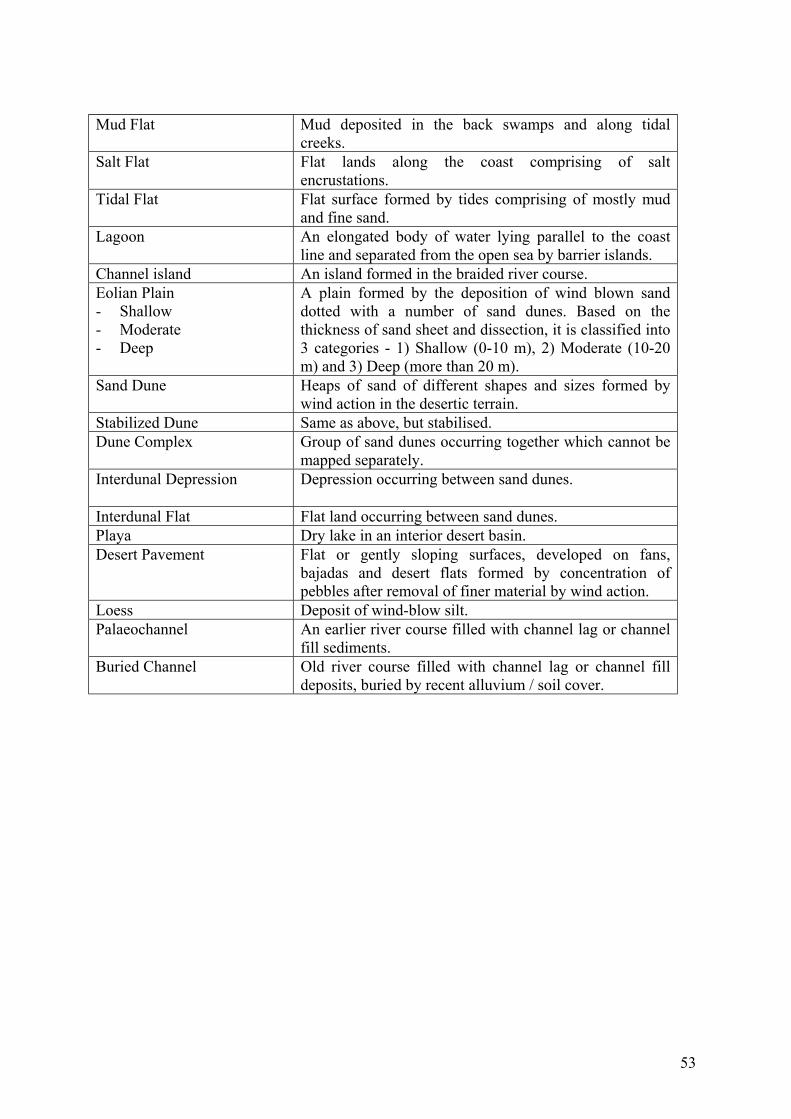
Mud Flat Mud deposited in the back swamps and along tidalcreeks.

Salt Flat Flat lands along the coast comprising of saltencrustations.

Tidal Flat Flat surface formed by tides comprising of mostly mudand fine sand.

Lagoon An elongated body of water lying parallel to the coastline and separated from the open sea by barrier islands.

Channel island An island formed in the braided river course.Eolian Plain- Shallow- Moderate- Deep

A plain formed by the deposition of wind blown sanddotted with a number of sand dunes. Based on thethickness of sand sheet and dissection, it is classified into3 categories - 1) Shallow (0-10 m), 2) Moderate (10-20m) and 3) Deep (more than 20 m).

Sand Dune Heaps of sand of different shapes and sizes formed bywind action in the desertic terrain.

Stabilized Dune Same as above, but stabilised.Dune Complex Group of sand dunes occurring together which cannot be

mapped separately.Interdunal Depression Depression occurring between sand dunes.

Interdunal Flat Flat land occurring between sand dunes.Playa Dry lake in an interior desert basin.Desert Pavement Flat or gently sloping surfaces, developed on fans,

bajadas and desert flats formed by concentration ofpebbles after removal of finer material by wind action.

Loess Deposit of wind-blow silt.Palaeochannel An earlier river course filled with channel lag or channel

fill sediments.Buried Channel Old river course filled with channel lag or channel fill

deposits, buried by recent alluvium / soil cover.

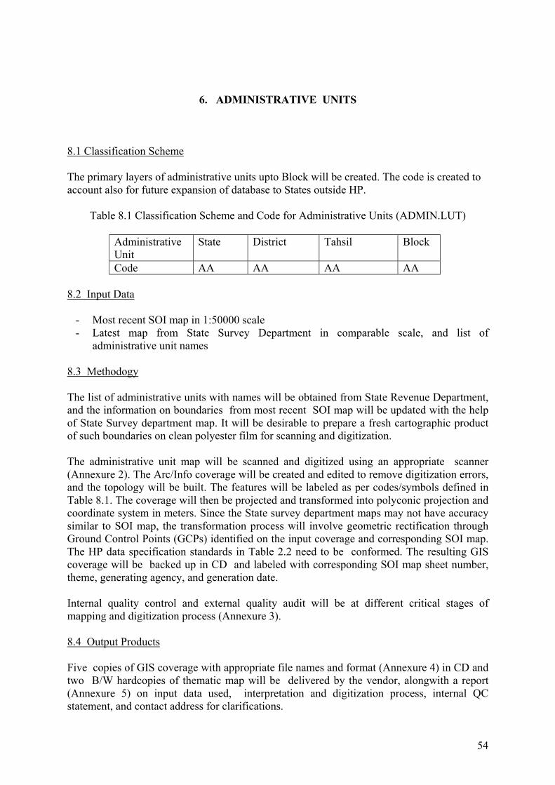
54

6. ADMINISTRATIVE UNITS


The primary layers of administrative units upto Block will be created. The code is created toaccount also for future expansion of database to States outside HP.

Table 8.1 Classification Scheme and Code for Administrative Units (ADMIN.LUT)

AdministrativeUnit

State District Tahsil Block

Code AA AA AA AA

8.2 Input Data

- Most recent SOI map in 1:50000 scale- Latest map from State Survey Department in comparable scale, and list of

administrative unit names

8.3 Methodogy

The list of administrative units with names will be obtained from State Revenue Department,and the information on boundaries from most recent SOI map will be updated with the helpof State Survey department map. It will be desirable to prepare a fresh cartographic productof such boundaries on clean polyester film for scanning and digitization.

The administrative unit map will be scanned and digitized using an appropriate scanner(Annexure 2). The Arc/Info coverage will be created and edited to remove digitization errors,and the topology will be built. The features will be labeled as per codes/symbols defined inTable 8.1. The coverage will then be projected and transformed into polyconic projection andcoordinate system in meters. Since the State survey department maps may not have accuracysimilar to SOI map, the transformation process will involve geometric rectification throughGround Control Points (GCPs) identified on the input coverage and corresponding SOI map.The HP data specification standards in Table 2.2 need to be conformed. The resulting GIScoverage will be backed up in CD and labeled with corresponding SOI map sheet number,theme, generating agency, and generation date.


8.4 Output Products


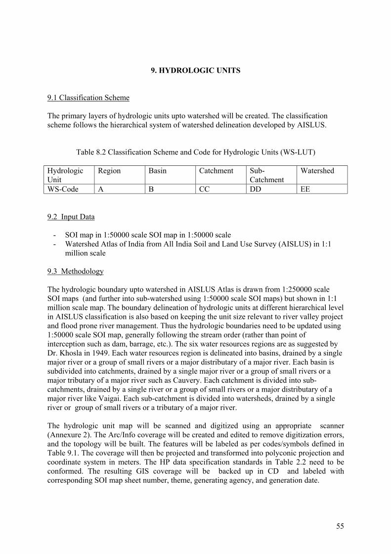
55

9. HYDROLOGIC UNITS


The primary layers of hydrologic units upto watershed will be created. The classificationscheme follows the hierarchical system of watershed delineation developed by AISLUS.

Table 8.2 Classification Scheme and Code for Hydrologic Units (WS-LUT)

HydrologicUnit

Region Basin Catchment Sub-Catchment

Watershed

WS-Code A B CC DD EE

9.2 Input Data

- SOI map in 1:50000 scale SOI map in 1:50000 scale- Watershed Atlas of India from All India Soil and Land Use Survey (AISLUS) in 1:1

million scale

9.3 Methodology

The hydrologic boundary upto watershed in AISLUS Atlas is drawn from 1:250000 scaleSOI maps (and further into sub-watershed using 1:50000 scale SOI maps) but shown in 1:1million scale map. The boundary delineation of hydrologic units at different hierarchical levelin AISLUS classification is also based on keeping the unit size relevant to river valley projectand flood prone river management. Thus the hydrologic boundaries need to be updated using1:50000 scale SOI map, generally following the stream order (rather than point ofinterception such as dam, barrage, etc.). The six water resources regions are as suggested byDr. Khosla in 1949. Each water resources region is delineated into basins, drained by a singlemajor river or a group of small rivers or a major distributary of a major river. Each basin issubdivided into catchments, drained by a single major river or a group of small rivers or amajor tributary of a major river such as Cauvery. Each catchment is divided into sub-catchments, drained by a single river or a group of small rivers or a major distributary of amajor river like Vaigai. Each sub-catchment is divided into watersheds, drained by a singleriver or group of small rivers or a tributary of a major river.

The hydrologic unit map will be scanned and digitized using an appropriate scanner(Annexure 2). The Arc/Info coverage will be created and edited to remove digitization errors,and the topology will be built. The features will be labeled as per codes/symbols defined inTable 9.1. The coverage will then be projected and transformed into polyconic projection andcoordinate system in meters. The HP data specification standards in Table 2.2 need to beconformed. The resulting GIS coverage will be backed up in CD and labeled withcorresponding SOI map sheet number, theme, generating agency, and generation date.

56


9.4 Output Products


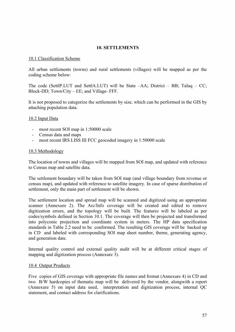
57

10. SETTLEMENTS


All urban settlements (towns) and rural settlements (villages) will be mapped as per thecoding scheme below:

The code (SettlP.LUT and SettlA.LUT) will be State –AA; District – BB; Taluq – CC;Block-DD; Town/City – EE; and Village- FFF.

It is not proposed to categorize the settlements by size, which can be performed in the GIS byattaching population data.

10.2 Input Data

- most recent SOI map in 1:50000 scale- Census data and maps- most recent IRS LISS III FCC geocoded imagery in 1:50000 scale

10.3 Methodology

The location of towns and villages will be mapped from SOI map, and updated with referenceto Census map and satellite data.

The settlement boundary will be taken from SOI map (and village boundary from revenue orcensus map), and updated with reference to satellite imagery. In case of sparse distribution ofsettlement, only the main part of settlement will be shown.

The settlement location and spread map will be scanned and digitized using an appropriatescanner (Annexure 2). The Arc/Info coverage will be created and edited to removedigitization errors, and the topology will be built. The features will be labeled as percodes/symbols defined in Section 10.1. The coverage will then be projected and transformedinto polyconic projection and coordinate system in meters. The HP data specificationstandards in Table 2.2 need to be conformed. The resulting GIS coverage will be backed upin CD and labeled with corresponding SOI map sheet number, theme, generating agency,and generation date.


10.4 Output Products


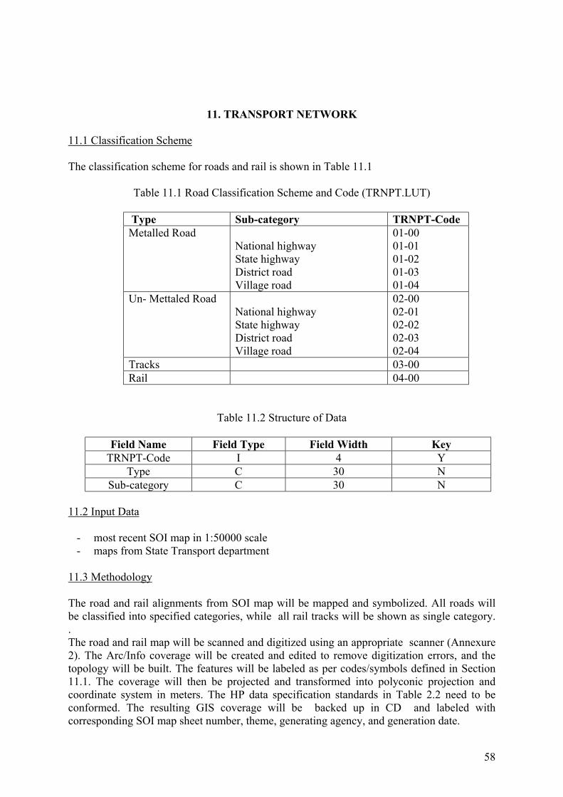
58

11. TRANSPORT NETWORK


The classification scheme for roads and rail is shown in Table 11.1

Table 11.1 Road Classification Scheme and Code (TRNPT.LUT)

Type Sub-category TRNPT-CodeMetalled Road

National highwayState highwayDistrict roadVillage road

01-0001-0101-0201-0301-04

Un- Mettaled RoadNational highwayState highwayDistrict roadVillage road

02-0002-0102-0202-0302-04

Tracks 03-00Rail 04-00


Field Name Field Type Field Width KeyTRNPT-Code I 4 Y

Type C 30 NSub-category C 30 N

11.2 Input Data

- most recent SOI map in 1:50000 scale- maps from State Transport department

11.3 Methodology

The road and rail alignments from SOI map will be mapped and symbolized. All roads willbe classified into specified categories, while all rail tracks will be shown as single category..The road and rail map will be scanned and digitized using an appropriate scanner (Annexure2). The Arc/Info coverage will be created and edited to remove digitization errors, and thetopology will be built. The features will be labeled as per codes/symbols defined in Section11.1. The coverage will then be projected and transformed into polyconic projection andcoordinate system in meters. The HP data specification standards in Table 2.2 need to beconformed. The resulting GIS coverage will be backed up in CD and labeled withcorresponding SOI map sheet number, theme, generating agency, and generation date.

59




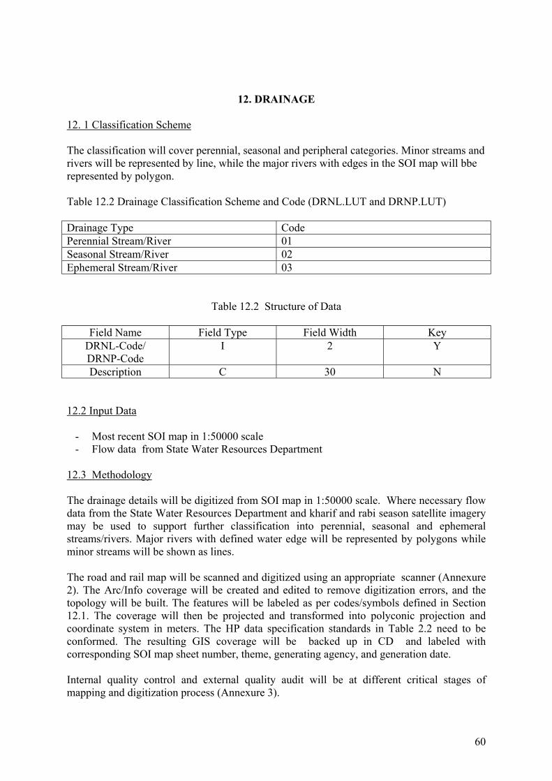
60

12. DRAINAGE

12. 1 Classification Scheme

The classification will cover perennial, seasonal and peripheral categories. Minor streams andrivers will be represented by line, while the major rivers with edges in the SOI map will bberepresented by polygon.

Table 12.2 Drainage Classification Scheme and Code (DRNL.LUT and DRNP.LUT)

Drainage Type CodePerennial Stream/River 01Seasonal Stream/River 02Ephemeral Stream/River 03


Field Name Field Type Field Width KeyDRNL-Code/DRNP-Code

I 2 Y

Description C 30 N

12.2 Input Data

- Most recent SOI map in 1:50000 scale- Flow data from State Water Resources Department

12.3 Methodology

The drainage details will be digitized from SOI map in 1:50000 scale. Where necessary flowdata from the State Water Resources Department and kharif and rabi season satellite imagerymay be used to support further classification into perennial, seasonal and ephemeralstreams/rivers. Major rivers with defined water edge will be represented by polygons whileminor streams will be shown as lines.

The road and rail map will be scanned and digitized using an appropriate scanner (Annexure2). The Arc/Info coverage will be created and edited to remove digitization errors, and thetopology will be built. The features will be labeled as per codes/symbols defined in Section12.1. The coverage will then be projected and transformed into polyconic projection andcoordinate system in meters. The HP data specification standards in Table 2.2 need to beconformed. The resulting GIS coverage will be backed up in CD and labeled withcorresponding SOI map sheet number, theme, generating agency, and generation date.


61



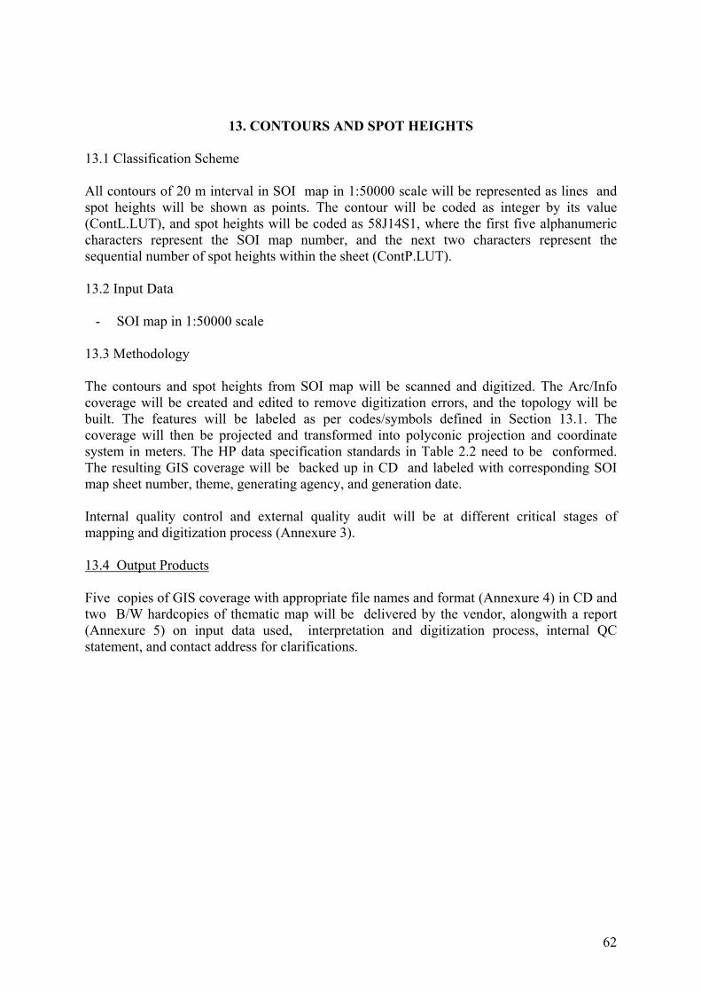
62

13. CONTOURS AND SPOT HEIGHTS


All contours of 20 m interval in SOI map in 1:50000 scale will be represented as lines andspot heights will be shown as points. The contour will be coded as integer by its value(ContL.LUT), and spot heights will be coded as 58J14S1, where the first five alphanumericcharacters represent the SOI map number, and the next two characters represent thesequential number of spot heights within the sheet (ContP.LUT).

13.2 Input Data

- SOI map in 1:50000 scale

13.3 Methodology

The contours and spot heights from SOI map will be scanned and digitized. The Arc/Infocoverage will be created and edited to remove digitization errors, and the topology will bebuilt. The features will be labeled as per codes/symbols defined in Section 13.1. Thecoverage will then be projected and transformed into polyconic projection and coordinatesystem in meters. The HP data specification standards in Table 2.2 need to be conformed.The resulting GIS coverage will be backed up in CD and labeled with corresponding SOImap sheet number, theme, generating agency, and generation date.




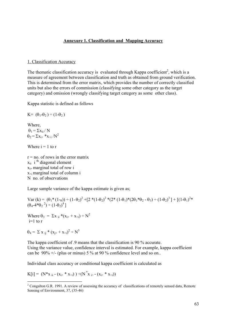
63

Annexure 1. Classification and Mapping Accuracy

1. Classification Accuracy

The thematic classification accuracy is evaluated through Kappa coefficient2, which is ameasure of agreement between classification and truth as obtained from ground verification.This is determined from the error matrix, which provides the number of correctly classifiedunits but also the errors of commission (classifying some other category as the targetcategory) and omission (wrongly classifying target category as some other class).

Kappa statistic is defined as follows

K= (θ1-θ2 ) ÷ (1-θ2 )

Where, θ1 = Σxii / Nθ2 = Σxi+ *x+i /N

2

Where i = 1 to r

r = no. of rows in the error matrixxii i

th diagonal elementxi+ marginal total of row ix+i marginal total of column iN no. of observations

Large sample variance of the kappa estimate is given as;

Var (k) = (θ1* (1-θ)) ÷ (1- θ2)2 +[2 *(1-θ2)

2 *(2* (1-θ1)*(2θ1*θ2 - θ3) ÷ (1-θ2)3 ] + [(1-θ1)

2*(θ4-4*θ2

2) ÷ (1-θ2)4 ]

Where θ3 = Σx ii *(xi+ + x+i) ÷ N2

i=1 to r

θ4 = Σ x ij * (xj+ + x+i)2 ÷ N3

The kappa coefficient of .9 means that the classification is 90 % accurate.Using the variance value, confidence interval is estimated. For example, kappa coefficientcan be 90% +/- (plus or minus) 5 % at 90 % confidence level and so on..

Individual class accuracy or conditional kappa coefficient is calculated as

K[i] = (N*x ii - (xi+ * x+i) ) ÷(N *x i+ - (xi+ * x+i))

2 Congalton G.R. 1991. A review of assessing the accuracy of classifications of remotely sensed data, RemoteSensing of Environment, 37, (35-46)

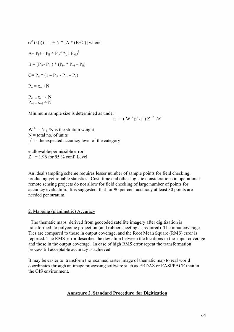
64

σ2 (k(i)) = 1 ÷ N * [A * (B+C)] where

A= Pi+ - Pii ÷ Pi+3 *(1-P+i)

3

B = (Pi+- Pii ) * (Pi+ * P+i – Pii)

C= Pii * (1 – Pi+ - P+i – Pii)

Pii = xii ÷N

Pi+ = xi+ ÷ NP+i = x+i ÷ N

Minimum sample size is determined as under n = ( W h ph qh ) Z�

2 /e2

W h = N h /N is the stratum weightN = total no. of unitsph is the expected accuracy level of the category

e allowable/permissible errorZ� = 1.96 for 95 % conf. Level

An ideal sampling scheme requires lesser number of sample points for field checking,producing yet reliable statistics. Cost, time and other logistic considerations in operationalremote sensing projects do not allow for field checking of large number of points foraccuracy evaluation. It is suggested that for 90 per cent accuracy at least 30 points areneeded per stratum.

2. Mapping (planimetric) Accuracy

The thematic maps derived from geocoded satellite imagery after digitization istransformed to polyconic projection (and rubber sheeting as required). The input coverageTics are compared to those in output coverage, and the Root Mean Square (RMS) error isreported. The RMS error describes the deviation between the locations in the input coverageand those in the output coverage. In case of high RMS error repeat the transformationprocess till acceptable accuracy is achieved.

It may be easier to transform the scanned raster image of thematic map to real worldcoordinates through an image processing software such as ERDAS or EASI/PACE than inthe GIS environment.

Annexure 2. Standard Procedure for Digitization

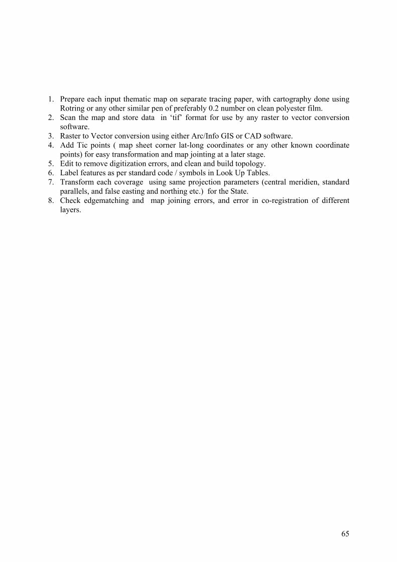
65

1. Prepare each input thematic map on separate tracing paper, with cartography done usingRotring or any other similar pen of preferably 0.2 number on clean polyester film.

2. Scan the map and store data in ‘tif’ format for use by any raster to vector conversionsoftware.

3. Raster to Vector conversion using either Arc/Info GIS or CAD software.4. Add Tic points ( map sheet corner lat-long coordinates or any other known coordinate

points) for easy transformation and map jointing at a later stage.5. Edit to remove digitization errors, and clean and build topology.6. Label features as per standard code / symbols in Look Up Tables.7. Transform each coverage using same projection parameters (central meridien, standard

parallels, and false easting and northing etc.) for the State.8. Check edgematching and map joining errors, and error in co-registration of different

layers.

66

Annexure 3 Internal Quality Assessment and External Quality Audit

Generation of standard and consistent data sets by multiple vendors in different locationsrequire that rigorous quality control is exercised internally and through independent externalaudit. Internal Quality Assurance procedures will cover different critical stages in data setgeneration, starting from appropriate satellite and other map input data selection, thematicinterpretation and validation, and final map validation. The stages in digitization process willcover scanning and digitization, labeling and attribute tables, and product labeling andreporting. Quality assessment will involve both visual inspection and measurements. Thevendor will develop a comprehensive QA procedure and report compliance. While internalQA will cover each data product, external QA will be on sampling basis.

A check list of parameters to be assessed at each stage will be prepared and completed andattached to the report accompanying the product. For example the data selection assessmentwill involve the parameters of year and seasons of satellite data, sensor, and area coveragecorresponding to specified SOI map.

The QC report will also be accessible to the external QA team during visit to the vendor site.

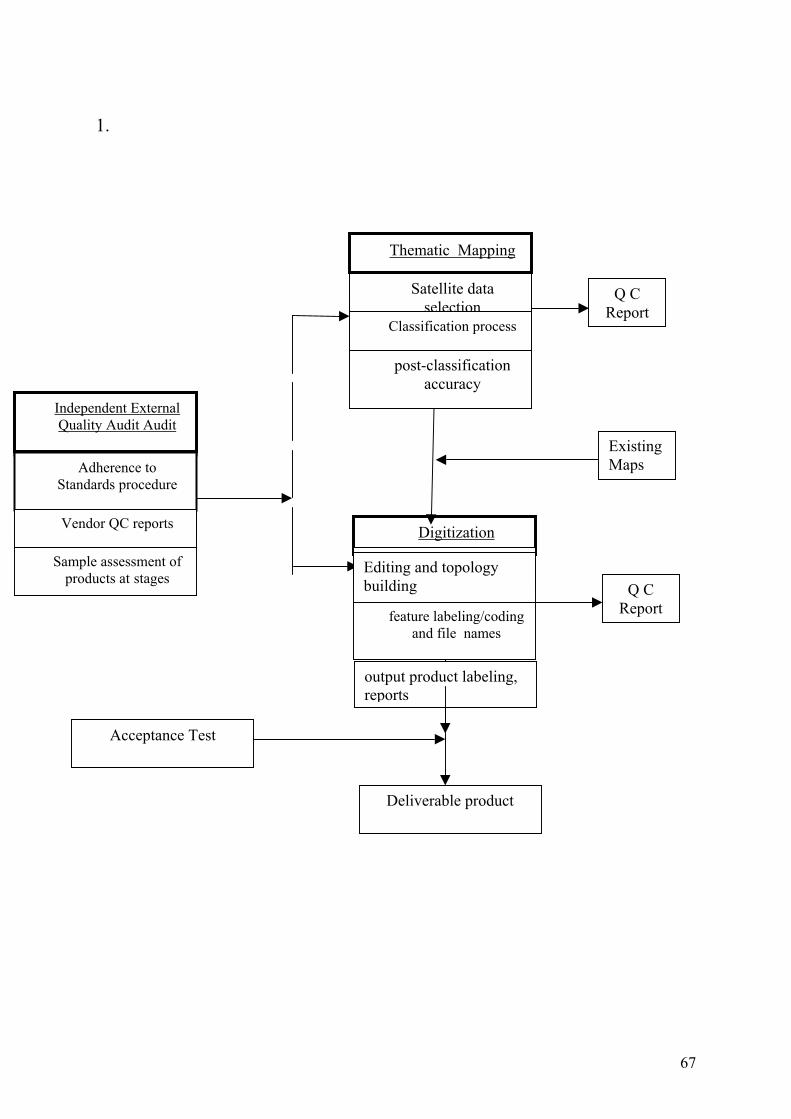
67

1.

Classification process

post-classificationaccuracy

Digitization

feature labeling/codingand file names

Adherence toStandards procedure

Vendor QC reports

Sample assessmentof products at major

Thematic Mapping

Satellite dataselection

Classification process

post-classificationaccuracy

Q CReport

Editing and topologybuilding

feature labeling/codingand file names

output product labeling,reports

Independent ExternalQuality Audit Audit

Adherence toStandards procedure

Vendor QC reports

Sample assessment ofproducts at stages

ExistingMaps

Q CReport

Deliverable product

Acceptance Test

Documents

Methodology Manual for Fresh Generation of Thematic Mapscwc.gov.in/main/HP/download/Spatial data sets Manual.pdf · 3 products. It is proposed to conduct orientation workshops for