Embed Size (px)
Citation preview
A P T I 4 3 5 : A T M O S P H E R I C S A M P L I N G C O U R S E
5-1
Methodologies and Instrumentation
for Particulate Matter Sampling
5.1 Introduction
In this chapter, the sampling principles discussed in Chapter 4 are applied to a discussion of the design and operation of PM samplers commonly used at monitoring sites, as well as PM samplers developed to accommodate other sampling needs. Specifically, Federal Reference Method (FRM) methods are discussed for TSP (today used primarily to monitor ambient lead and air toxics), PM10, PM2.5, and PM10-PM2.5. In addition to the FRM methods, continuous monitoring instruments, several of which are approved as FEMs for PM10 and PM2.5, are discussed in this chapter. The continuous instruments are increasingly being utilized at monitoring locations due to their ability to provide time-resolved PM mass concentration. This chapter also discusses filter-based PM2.5 speciation samplers, which are capable of providing elemental or compound- specific particulate mass concentration.
5.2 High-Volume Sampling for Suspended
Particulate Matter (SPM) and Air Toxics
When air pollution control agencies attempt to determine the nature and magnitude of air pollution in their communities and the effectiveness of their control programs, they collect samples of suspended, inhalable, and respirable particulate matter (PM). Suspended particulate matter (SPM) in air generally is a complex, multi-phase system of all airborne solid and low-vapor pressure liquid particles having aerodynamic particle sizes from below 0.01 μm to 100 μm and larger. Inhalable PM is the fraction of suspended particulate matter (SPM) that is capable of being respired into the human respiratory system in significant quantities, described as particles with an aerodynamic diameter of less than 10 µm (i.e., PM10). This size fraction is more commonly referred to as coarse particles or thoracic coarse particles. Another subset of SPM includes a size fraction of
Chapter
5
This chapter will take approximately 3.5 hours
to complete.
O B J E C T I V E S
Terminal Learning Objective
At the end of the chapter, the student will be able to describe the methods and
instruments used in particulate matter sampling.
Enabling Learning Objectives
5.1 Understand overview of chapter.
5.2 Describe high-volume sampling for suspended particulate matter (SPM) and air toxics.
5.3 Describe high-volume air sampling.
5.4 Describe the FRM for the determination of particulate matter as PM10.
5.5 Identify the FRM and FEM for the determination of fine particulate matter as PM2.5.
5.6 Identify the FRM and FEM for the determination of coarse particles (PM10-PM2.5).
5.7 Describe the procedures for PM2.5
speciation sampling. 5.8 Explain the procedures
for in situ monitoring for particulate matter.
5.9 Describe automated Federal Equivalent Monitors.
5.10 Describe additional automated PM methods.
A P T I 4 3 5 : A T M O S P H E R I C S A M P L I N G C O U R S E
5-2
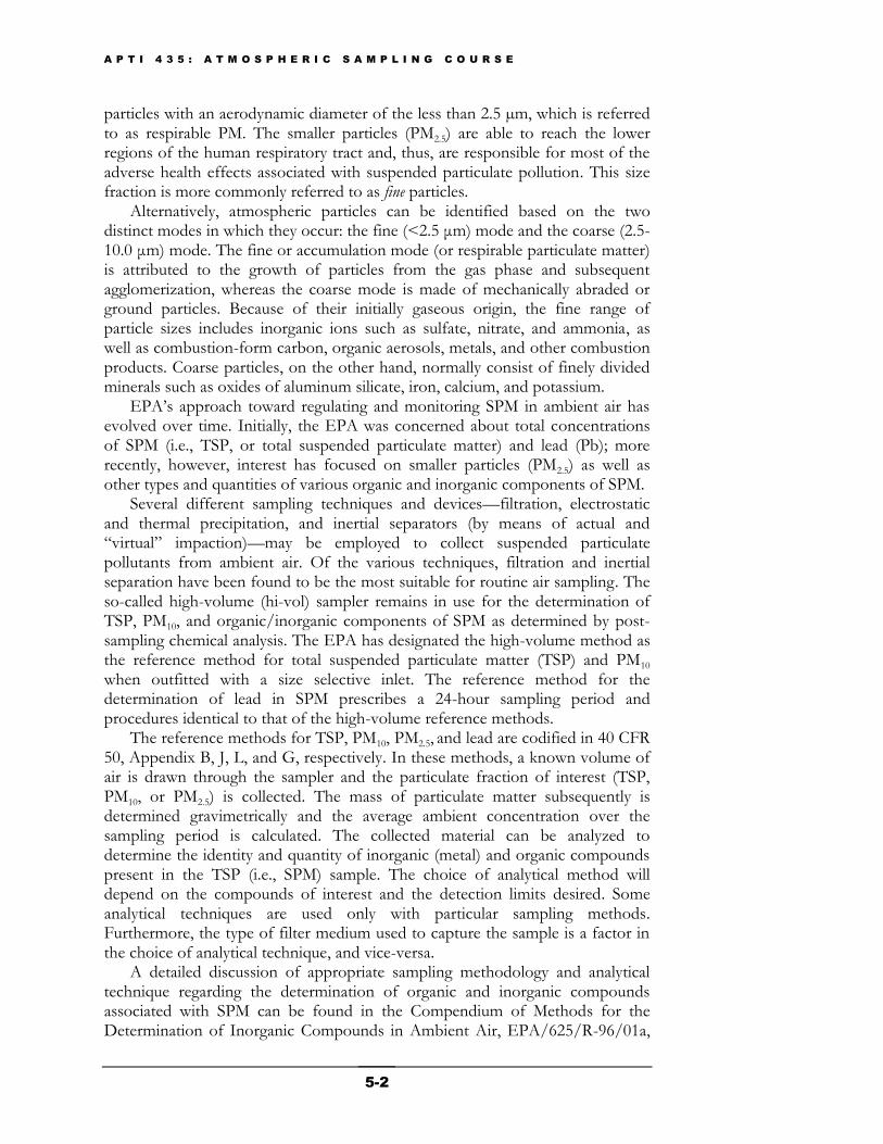
particles with an aerodynamic diameter of the less than 2.5 µm, which is referred to as respirable PM. The smaller particles (PM2.5) are able to reach the lower regions of the human respiratory tract and, thus, are responsible for most of the adverse health effects associated with suspended particulate pollution. This size fraction is more commonly referred to as fine particles.
Alternatively, atmospheric particles can be identified based on the two distinct modes in which they occur: the fine (<2.5 μm) mode and the coarse (2.5-10.0 μm) mode. The fine or accumulation mode (or respirable particulate matter) is attributed to the growth of particles from the gas phase and subsequent agglomerization, whereas the coarse mode is made of mechanically abraded or ground particles. Because of their initially gaseous origin, the fine range of particle sizes includes inorganic ions such as sulfate, nitrate, and ammonia, as well as combustion-form carbon, organic aerosols, metals, and other combustion products. Coarse particles, on the other hand, normally consist of finely divided minerals such as oxides of aluminum silicate, iron, calcium, and potassium.
EPA’s approach toward regulating and monitoring SPM in ambient air has evolved over time. Initially, the EPA was concerned about total concentrations of SPM (i.e., TSP, or total suspended particulate matter) and lead (Pb); more recently, however, interest has focused on smaller particles (PM2.5) as well as other types and quantities of various organic and inorganic components of SPM.
Several different sampling techniques and devices—filtration, electrostatic and thermal precipitation, and inertial separators (by means of actual and ―virtual‖ impaction)—may be employed to collect suspended particulate pollutants from ambient air. Of the various techniques, filtration and inertial separation have been found to be the most suitable for routine air sampling. The so-called high-volume (hi-vol) sampler remains in use for the determination of TSP, PM10, and organic/inorganic components of SPM as determined by post-sampling chemical analysis. The EPA has designated the high-volume method as the reference method for total suspended particulate matter (TSP) and PM10 when outfitted with a size selective inlet. The reference method for the determination of lead in SPM prescribes a 24-hour sampling period and procedures identical to that of the high-volume reference methods.
The reference methods for TSP, PM10, PM2.5, and lead are codified in 40 CFR 50, Appendix B, J, L, and G, respectively. In these methods, a known volume of air is drawn through the sampler and the particulate fraction of interest (TSP, PM10, or PM2.5) is collected. The mass of particulate matter subsequently is determined gravimetrically and the average ambient concentration over the sampling period is calculated. The collected material can be analyzed to determine the identity and quantity of inorganic (metal) and organic compounds present in the TSP (i.e., SPM) sample. The choice of analytical method will depend on the compounds of interest and the detection limits desired. Some analytical techniques are used only with particular sampling methods. Furthermore, the type of filter medium used to capture the sample is a factor in the choice of analytical technique, and vice-versa.
A detailed discussion of appropriate sampling methodology and analytical technique regarding the determination of organic and inorganic compounds associated with SPM can be found in the Compendium of Methods for the Determination of Inorganic Compounds in Ambient Air, EPA/625/R-96/01a,
A P T I 4 3 5 : A T M O S P H E R I C S A M P L I N G C O U R S E
5-3
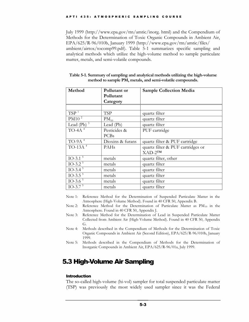
July 1999 (http://www.epa.gov/ttn/amtic/inorg. html) and the Compendium of Methods for the Determination of Toxic Organic Compounds in Ambient Air, EPA/625/R-96/010b, January 1999 (http://www.epa.gov/ttn/amtic/files/ ambient/airtox/tocomp99.pdf). Table 5-1 summarizes specific sampling and analytical methods which utilize the high-volume method to sample particulate matter, metals, and semi-volatile compounds.
Table 5-1. Summary of sampling and analytical methods utilizing the high-volume method to sample PM, metals, and semi-volatile compounds.
Method Pollutant or Pollutant Category
Sample Collection Media
TSP 1 TSP quartz filter
PM10 2 PM10 quartz filter
Lead (Pb) 3 Lead (Pb) quartz filter
TO-4A 4 Pesticides & PCBs
PUF cartridge
TO-9A 4 Dioxins & furans quartz filter & PUF cartridge
TO-13A 4 PAHs quartz filter & PUF cartridges or XAD-2™
IO-3.1 5 metals quartz filter, other
IO-3.2 5 metals quartz filter
IO-3.4 5 metals quartz filter
IO-3.5 5 metals quartz filter
IO-3.6 5 metals quartz filter
IO-3.7 5 metals quartz filter Note 1: Reference Method for the Determination of Suspended Particulate Matter in the
Atmosphere (High-Volume Method). Found in 40 CFR 50, Appendix B. Note 2: Reference Method for the Determination of Particulate Matter as PM10 in the
Atmosphere. Found in 40 CFR 50, Appendix J. Note 3: Reference Method for the Determination of Lead in Suspended Particulate Matter
Collected from Ambient Air (High-Volume Method). Found in 40 CFR 50, Appendix G.
Note 4: Methods described in the Compendium of Methods for the Determination of Toxic Organic Compounds in Ambient Air (Second Edition), EPA/625/R-96/010b, January 1999.
Note 5: Methods described in the Compendium of Methods for the Determination of Inorganic Compounds in Ambient Air, EPA/625/R-96/01a, July 1999.
5.3 High-Volume Air Sampling
Introduction
The so-called high-volume (hi-vol) sampler for total suspended particulate matter (TSP) was previously the most widely used sampler since it was the Federal
A P T I 4 3 5 : A T M O S P H E R I C S A M P L I N G C O U R S E
5-4
Reference Method (FRM) for measuring compliance with the TSP particulate matter standard. Approximately 20,000 hi-vols were operating at federal, state, and local air pollution control agencies, industries, and research organizations for either routine or intermittent use in the 1970’s. As TSP levels decreased, the number of TSP samplers in operation greatly diminished. With the promulgation of the PM10 standard in 1987, the number of TSP samplers operated by state and local agencies was down to approximately 2800 and the number of PM10 samplers was 636. By 1997 the number of TSP samplers operated by state and local control agencies was reduced to approximately 450. Although there is no TSP standard, the TSP FRM remains as the official sampling method for obtaining samples to determine compliance with the national ambient air quality standard for lead.
Development of the High-Volume Sampler
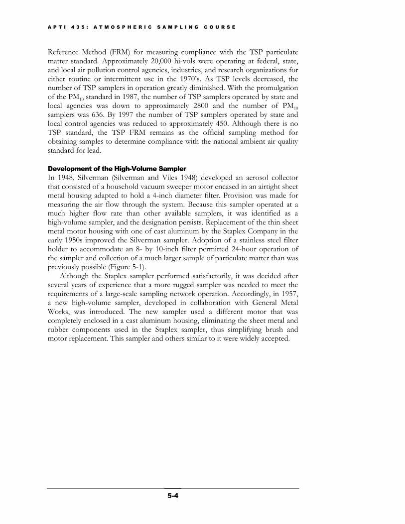
In 1948, Silverman (Silverman and Viles 1948) developed an aerosol collector that consisted of a household vacuum sweeper motor encased in an airtight sheet metal housing adapted to hold a 4-inch diameter filter. Provision was made for measuring the air flow through the system. Because this sampler operated at a much higher flow rate than other available samplers, it was identified as a high-volume sampler, and the designation persists. Replacement of the thin sheet metal motor housing with one of cast aluminum by the Staplex Company in the early 1950s improved the Silverman sampler. Adoption of a stainless steel filter holder to accommodate an 8- by 10-inch filter permitted 24-hour operation of the sampler and collection of a much larger sample of particulate matter than was previously possible (Figure 5-1).
Although the Staplex sampler performed satisfactorily, it was decided after several years of experience that a more rugged sampler was needed to meet the requirements of a large-scale sampling network operation. Accordingly, in 1957, a new high-volume sampler, developed in collaboration with General Metal Works, was introduced. The new sampler used a different motor that was completely enclosed in a cast aluminum housing, eliminating the sheet metal and rubber components used in the Staplex sampler, thus simplifying brush and motor replacement. This sampler and others similar to it were widely accepted.
A P T I 4 3 5 : A T M O S P H E R I C S A M P L I N G C O U R S E
5-5
Figure 5-1. Hi-vol sampler components (motor, filter, housing).
Sampler-Shelter Combination
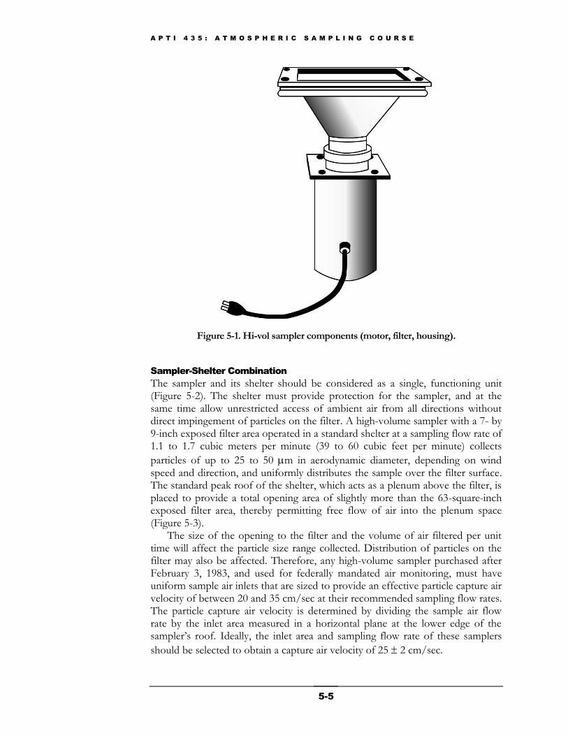
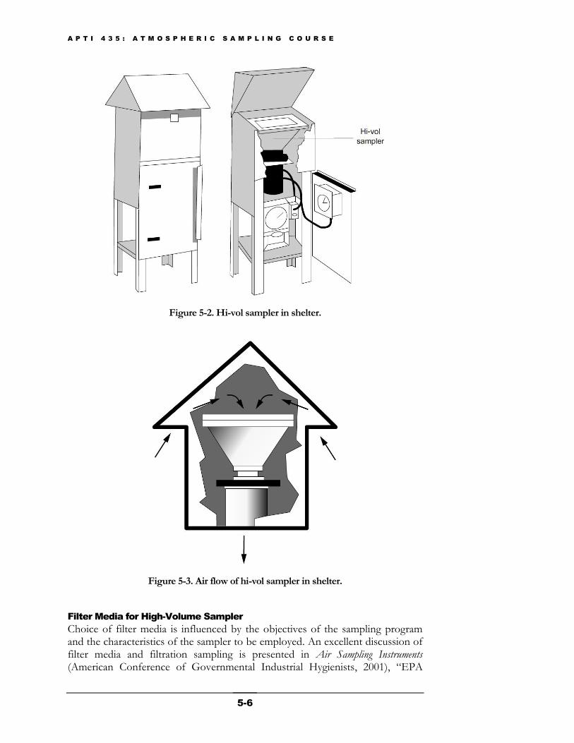
The sampler and its shelter should be considered as a single, functioning unit (Figure 5-2). The shelter must provide protection for the sampler, and at the same time allow unrestricted access of ambient air from all directions without direct impingement of particles on the filter. A high-volume sampler with a 7- by 9-inch exposed filter area operated in a standard shelter at a sampling flow rate of 1.1 to 1.7 cubic meters per minute (39 to 60 cubic feet per minute) collects
particles of up to 25 to 50 m in aerodynamic diameter, depending on wind speed and direction, and uniformly distributes the sample over the filter surface. The standard peak roof of the shelter, which acts as a plenum above the filter, is placed to provide a total opening area of slightly more than the 63-square-inch exposed filter area, thereby permitting free flow of air into the plenum space (Figure 5-3).
The size of the opening to the filter and the volume of air filtered per unit time will affect the particle size range collected. Distribution of particles on the filter may also be affected. Therefore, any high-volume sampler purchased after February 3, 1983, and used for federally mandated air monitoring, must have uniform sample air inlets that are sized to provide an effective particle capture air velocity of between 20 and 35 cm/sec at their recommended sampling flow rates. The particle capture air velocity is determined by dividing the sample air flow rate by the inlet area measured in a horizontal plane at the lower edge of the sampler’s roof. Ideally, the inlet area and sampling flow rate of these samplers
should be selected to obtain a capture air velocity of 25 2 cm/sec.
A P T I 4 3 5 : A T M O S P H E R I C S A M P L I N G C O U R S E
5-6
Figure 5-2. Hi-vol sampler in shelter.
Figure 5-3. Air flow of hi-vol sampler in shelter.
Filter Media for High-Volume Sampler
Choice of filter media is influenced by the objectives of the sampling program and the characteristics of the sampler to be employed. An excellent discussion of filter media and filtration sampling is presented in Air Sampling Instruments (American Conference of Governmental Industrial Hygienists, 2001), ―EPA
A P T I 4 3 5 : A T M O S P H E R I C S A M P L I N G C O U R S E
5-7
Guideline on Speciated Particulate Monitoring‖ (1998, Draft), and Chapter 4 of this Student Manual.
Glass fiber filters have been extensively used for total suspended particulate matter sampling. Such filters have a collection efficiency of at least 99% for
particles having aerodynamic diameters of 0.3 m and larger, low resistance to air flow, and low affinity for moisture, all of which are distinct advantages during sampling. However, in order to eliminate possible weight errors due to small amounts of moisture, both unexposed and exposed filters should be equilibrated
between 15°C and 30°C with less than 3°C variation, at a relative humidity
below 50% with less than 5% variation, for 24 hours before weighing. Samples collected on glass fiber filters are suitable for the analysis of a variety
of organic pollutants and a large number of inorganic contaminants, including trace metals and several nonmetallic substances. Also, glass fiber filters are excellent for monitoring gross radioactivity. However, satisfactory analyses for materials already present in substantial amounts in the filter are not possible. A random, but statistically significant, sample of new filters should be analyzed to determine whether the filter blank concentration is high enough to interfere with a particular analysis. It is wise to obtain this information before purchasing large numbers of filters to avoid potential problems caused by high filter blanks.
While glass fiber filter material has been dominant in the measurement of total suspended particulate matter, numerous applications have been found for cellulose filters. Cellulose filters have relatively low metal content, making them a good choice for metals analysis by neutron activation, atomic absorption, emission spectroscopy, etc. Conventional high-volume samplers usually have to be modified to use cellulose filters because the filters clog rapidly, causing flow to sometimes decrease by as much as a factor of two during a one-day sampling interval. Other disadvantages of cellulose are its absorption of water and enhanced artifact formation of nitrates and sulfates. These disadvantages can usually be overcome by using a control blank filter. Spectro-quality grade glass fiber filters have sufficiently low background metal content to make them acceptable for metal analysis, if cellulose cannot be used.
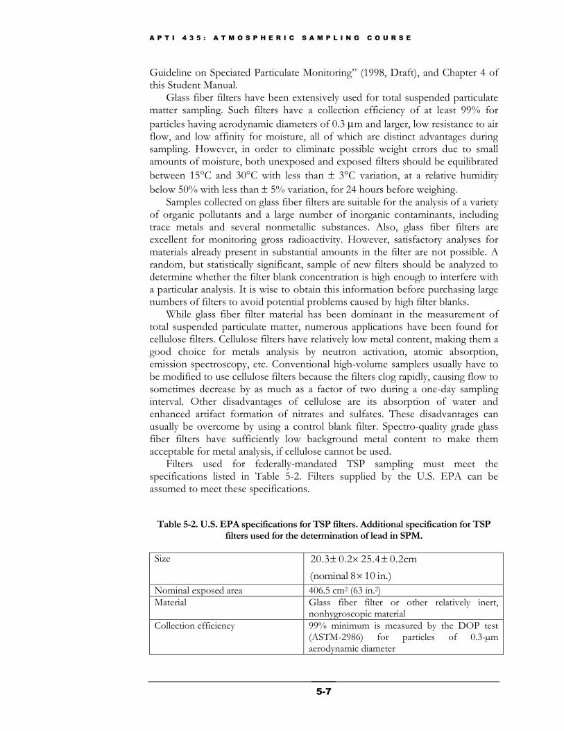
Filters used for federally-mandated TSP sampling must meet the specifications listed in Table 5-2. Filters supplied by the U.S. EPA can be assumed to meet these specifications.
Table 5-2. U.S. EPA specifications for TSP filters. Additional specification for TSP filters used for the determination of lead in SPM.
Size
in.)10 8(nominal
0.2cm25.40.220.3
Nominal exposed area 406.5 cm2 (63 in.2)
Material Glass fiber filter or other relatively inert, nonhygroscopic material
Collection efficiency 99% minimum is measured by the DOP test (ASTM-2986) for particles of 0.3-µm aerodynamic diameter
A P T I 4 3 5 : A T M O S P H E R I C S A M P L I N G C O U R S E
5-8
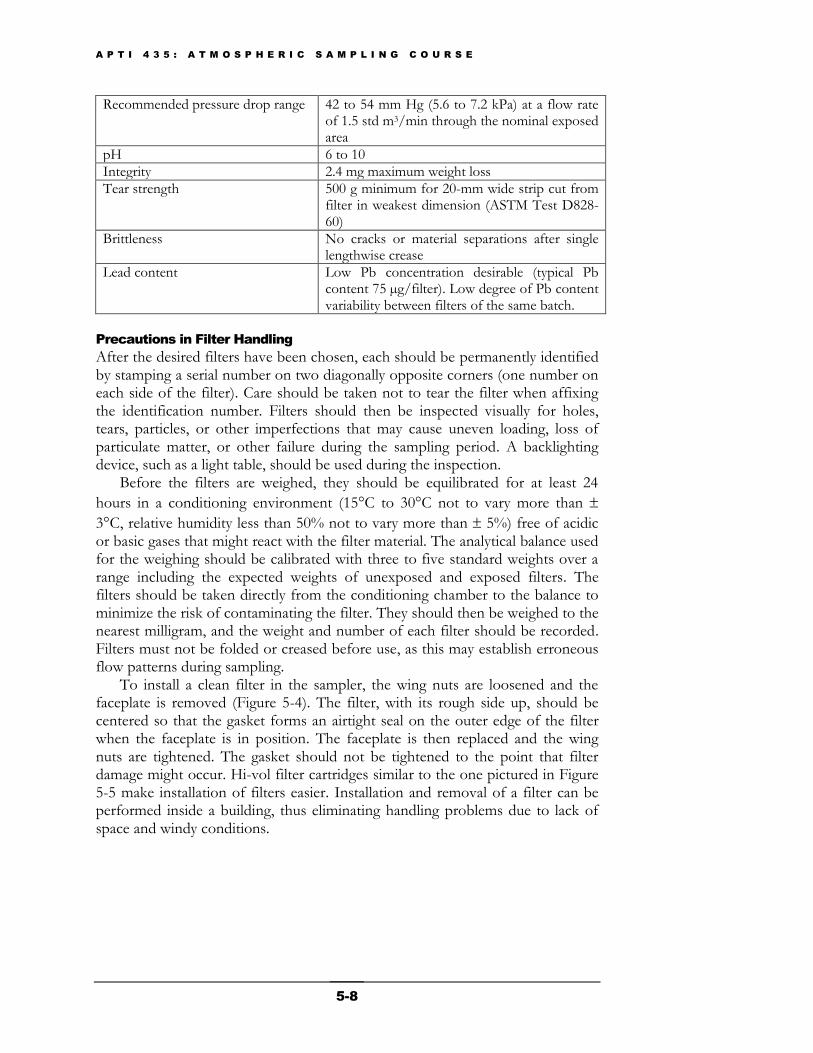
Recommended pressure drop range 42 to 54 mm Hg (5.6 to 7.2 kPa) at a flow rate of 1.5 std m3/min through the nominal exposed area
pH 6 to 10
Integrity 2.4 mg maximum weight loss
Tear strength 500 g minimum for 20-mm wide strip cut from filter in weakest dimension (ASTM Test D828-60)
Brittleness No cracks or material separations after single lengthwise crease
Lead content Low Pb concentration desirable (typical Pb content 75 µg/filter). Low degree of Pb content variability between filters of the same batch.
Precautions in Filter Handling
After the desired filters have been chosen, each should be permanently identified by stamping a serial number on two diagonally opposite corners (one number on each side of the filter). Care should be taken not to tear the filter when affixing the identification number. Filters should then be inspected visually for holes, tears, particles, or other imperfections that may cause uneven loading, loss of particulate matter, or other failure during the sampling period. A backlighting device, such as a light table, should be used during the inspection.
Before the filters are weighed, they should be equilibrated for at least 24
hours in a conditioning environment (15°C to 30°C not to vary more than
3°C, relative humidity less than 50% not to vary more than 5%) free of acidic or basic gases that might react with the filter material. The analytical balance used for the weighing should be calibrated with three to five standard weights over a range including the expected weights of unexposed and exposed filters. The filters should be taken directly from the conditioning chamber to the balance to minimize the risk of contaminating the filter. They should then be weighed to the nearest milligram, and the weight and number of each filter should be recorded. Filters must not be folded or creased before use, as this may establish erroneous flow patterns during sampling.
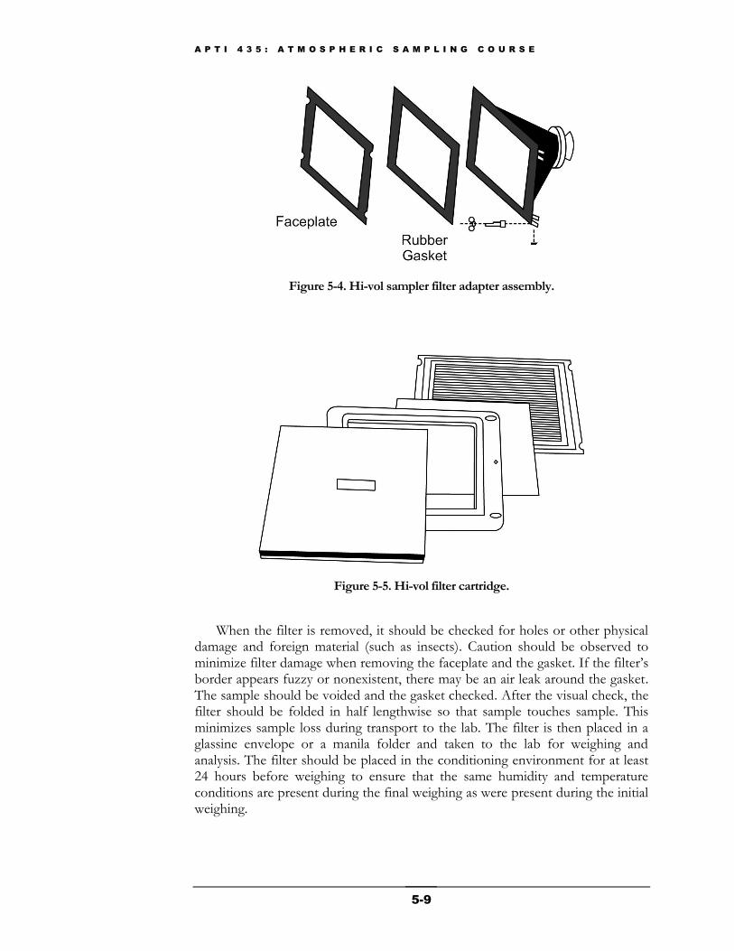
To install a clean filter in the sampler, the wing nuts are loosened and the faceplate is removed (Figure 5-4). The filter, with its rough side up, should be centered so that the gasket forms an airtight seal on the outer edge of the filter when the faceplate is in position. The faceplate is then replaced and the wing nuts are tightened. The gasket should not be tightened to the point that filter damage might occur. Hi-vol filter cartridges similar to the one pictured in Figure 5-5 make installation of filters easier. Installation and removal of a filter can be performed inside a building, thus eliminating handling problems due to lack of space and windy conditions.
A P T I 4 3 5 : A T M O S P H E R I C S A M P L I N G C O U R S E
5-9
Figure 5-4. Hi-vol sampler filter adapter assembly.
Figure 5-5. Hi-vol filter cartridge.
When the filter is removed, it should be checked for holes or other physical damage and foreign material (such as insects). Caution should be observed to minimize filter damage when removing the faceplate and the gasket. If the filter’s border appears fuzzy or nonexistent, there may be an air leak around the gasket. The sample should be voided and the gasket checked. After the visual check, the filter should be folded in half lengthwise so that sample touches sample. This minimizes sample loss during transport to the lab. The filter is then placed in a glassine envelope or a manila folder and taken to the lab for weighing and analysis. The filter should be placed in the conditioning environment for at least 24 hours before weighing to ensure that the same humidity and temperature conditions are present during the final weighing as were present during the initial weighing.
A P T I 4 3 5 : A T M O S P H E R I C S A M P L I N G C O U R S E
5-10
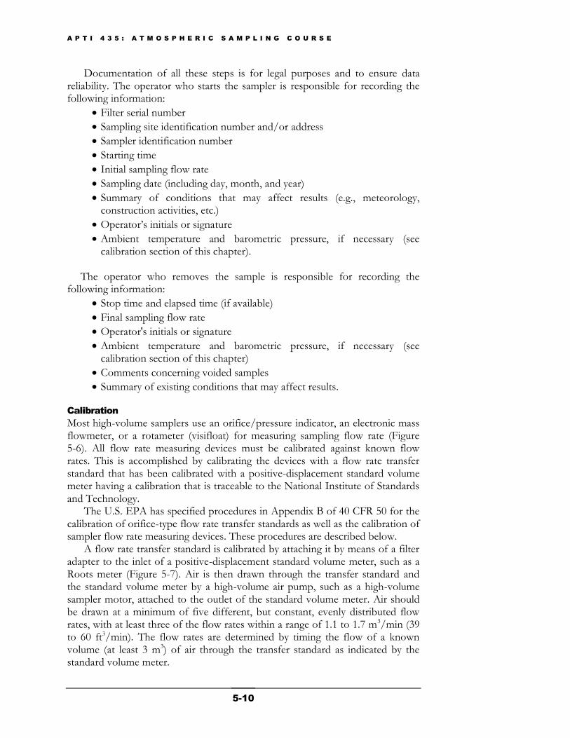
Documentation of all these steps is for legal purposes and to ensure data reliability. The operator who starts the sampler is responsible for recording the following information:
Filter serial number
Sampling site identification number and/or address
Sampler identification number
Starting time
Initial sampling flow rate
Sampling date (including day, month, and year)
Summary of conditions that may affect results (e.g., meteorology, construction activities, etc.)
Operator’s initials or signature
Ambient temperature and barometric pressure, if necessary (see calibration section of this chapter).
The operator who removes the sample is responsible for recording the following information:
Stop time and elapsed time (if available)
Final sampling flow rate
Operator's initials or signature
Ambient temperature and barometric pressure, if necessary (see calibration section of this chapter)
Comments concerning voided samples
Summary of existing conditions that may affect results.
Calibration
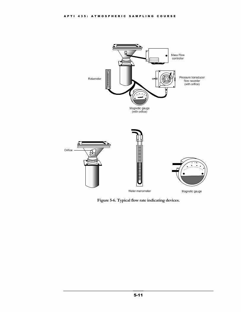
Most high-volume samplers use an orifice/pressure indicator, an electronic mass flowmeter, or a rotameter (visifloat) for measuring sampling flow rate (Figure 5-6). All flow rate measuring devices must be calibrated against known flow rates. This is accomplished by calibrating the devices with a flow rate transfer standard that has been calibrated with a positive-displacement standard volume meter having a calibration that is traceable to the National Institute of Standards and Technology.
The U.S. EPA has specified procedures in Appendix B of 40 CFR 50 for the calibration of orifice-type flow rate transfer standards as well as the calibration of sampler flow rate measuring devices. These procedures are described below.
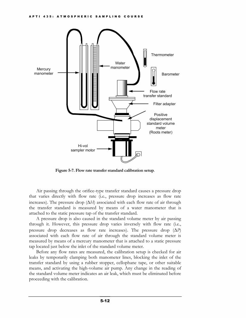
A flow rate transfer standard is calibrated by attaching it by means of a filter adapter to the inlet of a positive-displacement standard volume meter, such as a Roots meter (Figure 5-7). Air is then drawn through the transfer standard and the standard volume meter by a high-volume air pump, such as a high-volume sampler motor, attached to the outlet of the standard volume meter. Air should be drawn at a minimum of five different, but constant, evenly distributed flow rates, with at least three of the flow rates within a range of 1.1 to 1.7 m3/min (39 to 60 ft3/min). The flow rates are determined by timing the flow of a known volume (at least 3 m3) of air through the transfer standard as indicated by the standard volume meter.
A P T I 4 3 5 : A T M O S P H E R I C S A M P L I N G C O U R S E
5-11
Figure 5-6. Typical flow rate indicating devices.
A P T I 4 3 5 : A T M O S P H E R I C S A M P L I N G C O U R S E
5-12
Figure 5-7. Flow rate transfer standard calibration setup.
Air passing through the orifice-type transfer standard causes a pressure drop
that varies directly with flow rate (i.e., pressure drop increases as flow rate
increases). The pressure drop (H) associated with each flow rate of air through the transfer standard is measured by means of a water manometer that is attached to the static pressure tap of the transfer standard.
A pressure drop is also caused in the standard volume meter by air passing through it. However, this pressure drop varies inversely with flow rate (i.e.,
pressure drop decreases as flow rate increases). The pressure drop (P) associated with each flow rate of air through the standard volume meter is measured by means of a mercury manometer that is attached to a static pressure tap located just below the inlet of the standard volume meter.
Before any flow rates are measured, the calibration setup is checked for air leaks by temporarily clamping both manometer lines, blocking the inlet of the transfer standard by using a rubber stopper, cellophane tape, or other suitable means, and activating the high-volume air pump. Any change in the reading of the standard volume meter indicates an air leak, which must be eliminated before proceeding with the calibration.
A P T I 4 3 5 : A T M O S P H E R I C S A M P L I N G C O U R S E
5-13
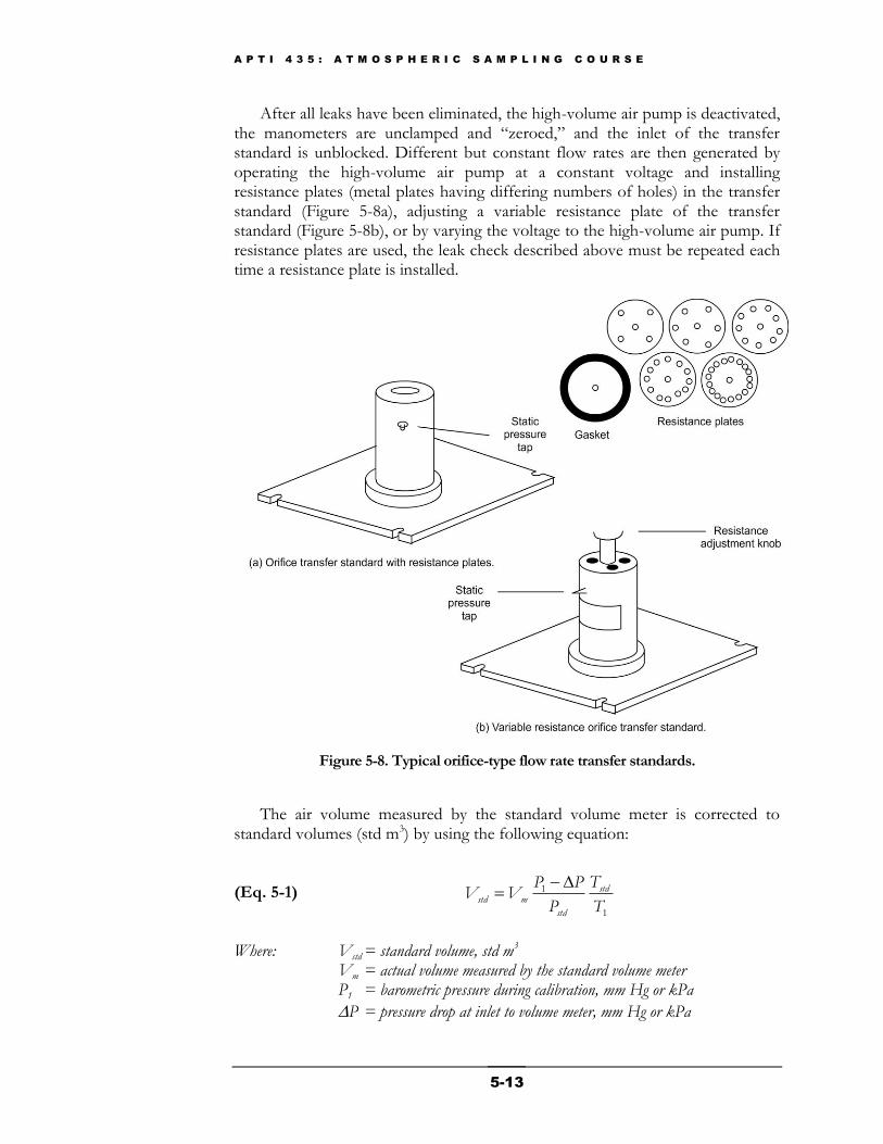
After all leaks have been eliminated, the high-volume air pump is deactivated, the manometers are unclamped and ―zeroed,‖ and the inlet of the transfer standard is unblocked. Different but constant flow rates are then generated by operating the high-volume air pump at a constant voltage and installing resistance plates (metal plates having differing numbers of holes) in the transfer standard (Figure 5-8a), adjusting a variable resistance plate of the transfer standard (Figure 5-8b), or by varying the voltage to the high-volume air pump. If resistance plates are used, the leak check described above must be repeated each time a resistance plate is installed.
Figure 5-8. Typical orifice-type flow rate transfer standards.
The air volume measured by the standard volume meter is corrected to standard volumes (std m3) by using the following equation:
(Eq. 5-1) Where: Vstd = standard volume, std m3 Vm = actual volume measured by the standard volume meter P1 = barometric pressure during calibration, mm Hg or kPa
P = pressure drop at inlet to volume meter, mm Hg or kPa
1
1
T
T
P
PPVV std
std
mstd
A P T I 4 3 5 : A T M O S P H E R I C S A M P L I N G C O U R S E
5-14
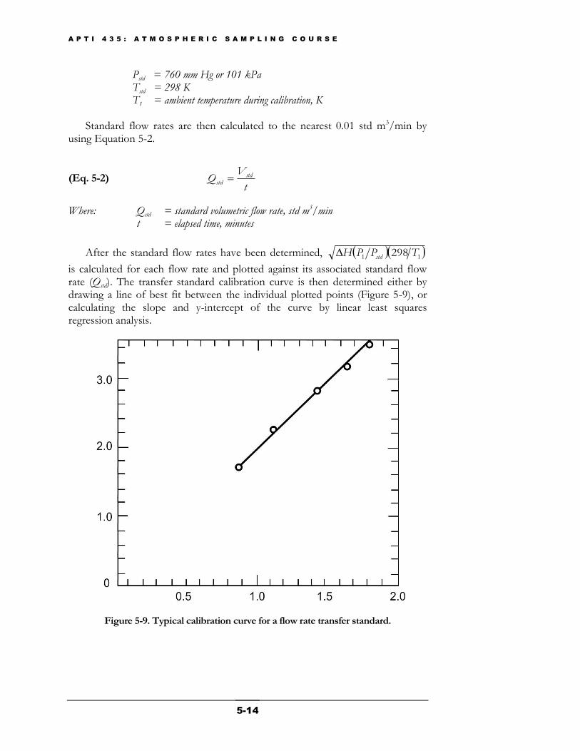
Pstd = 760 mm Hg or 101 kPa Tstd = 298 K T1 = ambient temperature during calibration, K
Standard flow rates are then calculated to the nearest 0.01 std m3/min by using Equation 5-2.
(Eq. 5-2) t
VQ std
std
Where: Qstd = standard volumetric flow rate, std m3/min t = elapsed time, minutes
After the standard flow rates have been determined, 11 298 TPPH std
is calculated for each flow rate and plotted against its associated standard flow rate (Qstd). The transfer standard calibration curve is then determined either by drawing a line of best fit between the individual plotted points (Figure 5-9), or calculating the slope and y-intercept of the curve by linear least squares regression analysis.
Figure 5-9. Typical calibration curve for a flow rate transfer standard.
A P T I 4 3 5 : A T M O S P H E R I C S A M P L I N G C O U R S E
5-15
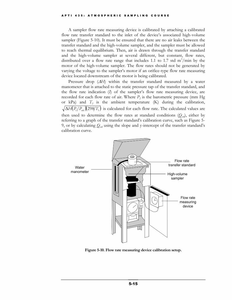
A sampler flow rate measuring device is calibrated by attaching a calibrated flow rate transfer standard to the inlet of the device’s associated high-volume sampler (Figure 5-10). It must be ensured that there are no air leaks between the transfer standard and the high-volume sampler, and the sampler must be allowed to reach thermal equilibrium. Then, air is drawn through the transfer standard and the high-volume sampler at several different, but constant, flow rates, distributed over a flow rate range that includes 1.1 to 1.7 std m3/min by the motor of the high-volume sampler. The flow rates should not be generated by varying the voltage to the sampler’s motor if an orifice-type flow rate measuring device located downstream of the motor is being calibrated.
Pressure drop (H) within the transfer standard measured by a water manometer that is attached to the static pressure tap of the transfer standard, and the flow rate indication (I) of the sampler’s flow rate measuring device, are recorded for each flow rate of air. Where P2 is the barometric pressure (mm Hg or kPa) and T2 is the ambient temperature (K) during the calibration,
11 298 TPPH std is calculated for each flow rate. The calculated values are
then used to determine the flow rates at standard conditions (Qstd), either by referring to a graph of the transfer standard’s calibration curve, such as Figure 5-9, or by calculating Qstd using the slope and y-intercept of the transfer standard’s calibration curve.
Figure 5-10. Flow rate measuring device calibration setup.
A P T I 4 3 5 : A T M O S P H E R I C S A M P L I N G C O U R S E
5-16
Flow rates indicated (I) by a sampler’s flow rate measuring device are then expressed, with regard to the type of flow rate measuring device used and the method of correcting sample air volumes for ambient temperature and barometric pressure, by using the formulas of Table 5-3. The formulas for geographic average barometric pressure (Pa) and seasonal average temperature (Ta) may be used to approximate actual pressure and temperature conditions during sampling for a seasonal period, if the actual barometric pressure and
temperature at the sampling site do not vary by more than 60 mm Hg from Pa
or 15°C from Ta , respectively. Furthermore, Pa may be estimated from an altitude-pressure table or by making an approximate elevation correction of -26 mm Hg (-3.46 kPa) for each 305 m (1000 ft) that the sampler is above sea level (760 mm Hg or 101 kPa), and Ta may be estimated from weather station or other records.
Table 5-3. Formulas for expressing indicated flow rates of sampler flow rate measuring device calibration.
Type of sampler flow rate measuring device
Expression
For actual pressure (P2) and temperature
(T2) corrections
For incorporation of geographic average
barometric pressure (Pa) and seasonal average
temperature (Ta)
Mass flowmeter I I
Orifice and pressure indicator
2std
2
T
298
P
PI
2
a
a
2
T
T
P
PI
Rotameter, or orifice and pressure recorder having a square root scale*
2std
2
T
298
P
PI
2
a
a
2
T
T
P
PI
* This scale is recognizable by its non-uniform divisions and is the most commonly available for
high-volume samplers.
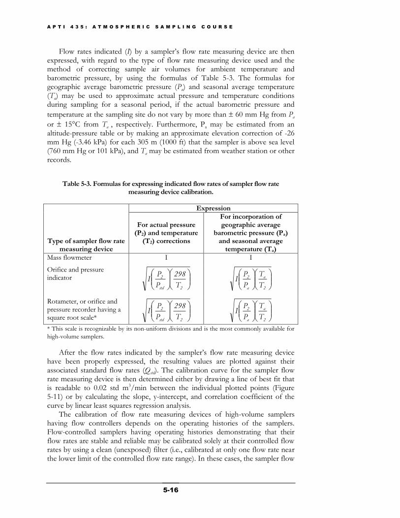
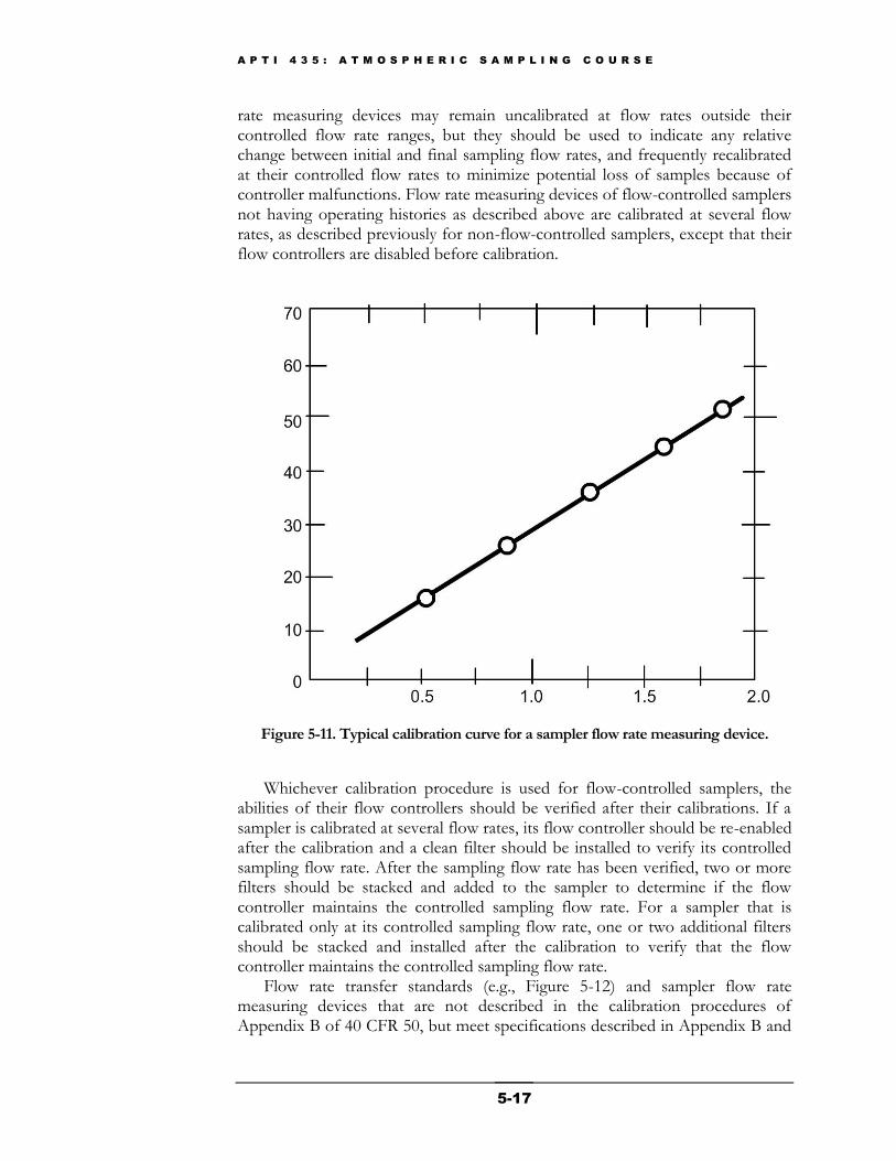
After the flow rates indicated by the sampler’s flow rate measuring device have been properly expressed, the resulting values are plotted against their associated standard flow rates (Qstd). The calibration curve for the sampler flow rate measuring device is then determined either by drawing a line of best fit that is readable to 0.02 std m3/min between the individual plotted points (Figure 5-11) or by calculating the slope, y-intercept, and correlation coefficient of the curve by linear least squares regression analysis.
The calibration of flow rate measuring devices of high-volume samplers having flow controllers depends on the operating histories of the samplers. Flow-controlled samplers having operating histories demonstrating that their flow rates are stable and reliable may be calibrated solely at their controlled flow rates by using a clean (unexposed) filter (i.e., calibrated at only one flow rate near the lower limit of the controlled flow rate range). In these cases, the sampler flow
A P T I 4 3 5 : A T M O S P H E R I C S A M P L I N G C O U R S E
5-17
rate measuring devices may remain uncalibrated at flow rates outside their controlled flow rate ranges, but they should be used to indicate any relative change between initial and final sampling flow rates, and frequently recalibrated at their controlled flow rates to minimize potential loss of samples because of controller malfunctions. Flow rate measuring devices of flow-controlled samplers not having operating histories as described above are calibrated at several flow rates, as described previously for non-flow-controlled samplers, except that their flow controllers are disabled before calibration.
Figure 5-11. Typical calibration curve for a sampler flow rate measuring device.
Whichever calibration procedure is used for flow-controlled samplers, the abilities of their flow controllers should be verified after their calibrations. If a sampler is calibrated at several flow rates, its flow controller should be re-enabled after the calibration and a clean filter should be installed to verify its controlled sampling flow rate. After the sampling flow rate has been verified, two or more filters should be stacked and added to the sampler to determine if the flow controller maintains the controlled sampling flow rate. For a sampler that is calibrated only at its controlled sampling flow rate, one or two additional filters should be stacked and installed after the calibration to verify that the flow controller maintains the controlled sampling flow rate.
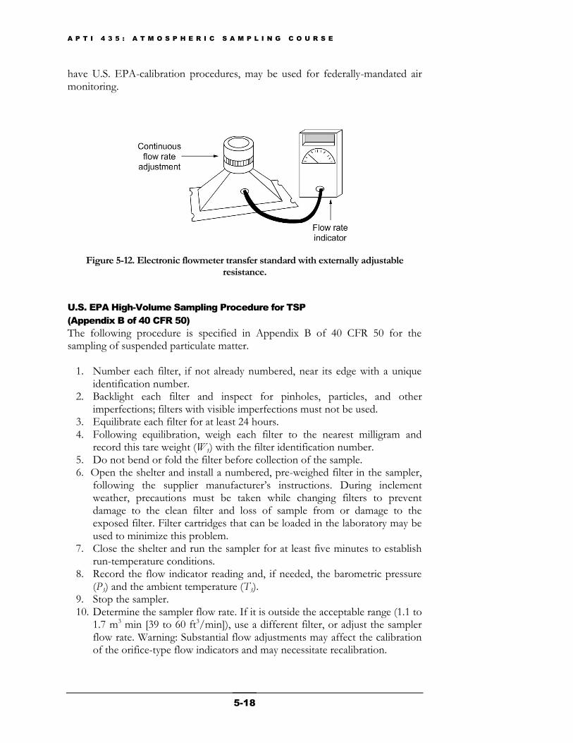
Flow rate transfer standards (e.g., Figure 5-12) and sampler flow rate measuring devices that are not described in the calibration procedures of Appendix B of 40 CFR 50, but meet specifications described in Appendix B and
A P T I 4 3 5 : A T M O S P H E R I C S A M P L I N G C O U R S E
5-18
have U.S. EPA-calibration procedures, may be used for federally-mandated air monitoring.
Figure 5-12. Electronic flowmeter transfer standard with externally adjustable resistance.
U.S. EPA High-Volume Sampling Procedure for TSP
(Appendix B of 40 CFR 50)
The following procedure is specified in Appendix B of 40 CFR 50 for the sampling of suspended particulate matter.
1. Number each filter, if not already numbered, near its edge with a unique identification number.
2. Backlight each filter and inspect for pinholes, particles, and other imperfections; filters with visible imperfections must not be used.
3. Equilibrate each filter for at least 24 hours. 4. Following equilibration, weigh each filter to the nearest milligram and
record this tare weight (W1) with the filter identification number. 5. Do not bend or fold the filter before collection of the sample. 6. Open the shelter and install a numbered, pre-weighed filter in the sampler,
following the supplier manufacturer’s instructions. During inclement weather, precautions must be taken while changing filters to prevent damage to the clean filter and loss of sample from or damage to the exposed filter. Filter cartridges that can be loaded in the laboratory may be used to minimize this problem.
7. Close the shelter and run the sampler for at least five minutes to establish run-temperature conditions.
8. Record the flow indicator reading and, if needed, the barometric pressure (P3) and the ambient temperature (T3).
9. Stop the sampler. 10. Determine the sampler flow rate. If it is outside the acceptable range (1.1 to
1.7 m3 min [39 to 60 ft3/min]), use a different filter, or adjust the sampler flow rate. Warning: Substantial flow adjustments may affect the calibration of the orifice-type flow indicators and may necessitate recalibration.
A P T I 4 3 5 : A T M O S P H E R I C S A M P L I N G C O U R S E
5-19
11. Record the sampler identification information (filter number, site location or identification number, sample date, and starting time).
12. Set the timer to start and stop the sampler so that the sampler runs 24 hours, from midnight to midnight (local time).
13. As soon as practical following the sampling period, run the sampler for at least five minutes to again establish run-temperature conditions.
14. Record the flow indicator reading and, if needed, the barometric pressure (P3) and the ambient temperature (T3).
Note: No onsite pressure or temperature measurements are necessary if the sampler flow indicator does not require pressure or temperature corrections (e.g., a mass flowmeter) or if average barometric pressure and seasonal average temperature for the site are incorporated into the sampler calibration. For individual pressure and temperature corrections, the ambient pressure and temperature can be obtained by onsite measurements or from a nearby weather station. Barometric pressure readings obtained from airports must be station pressure, not corrected to sea level, and may need to be corrected for differences in elevation between the sampler site and the airport. For a sampler having flow recorders but not constant flow controllers, the average temperature and pressure at the site during the sampling period should be estimated from weather bureau or other available data.
15. Stop the sampler and carefully remove the filter, following the sampler manufacturer's instructions. Touch only the outer edges of the filter.
16. Fold the filter in half lengthwise so that only surfaces with collected particulate matter are in contact and place it in the filter holder (glassine envelope or manila folder).
17. Record the ending time or elapsed time on the filter information record, either from the stop set point time, from an elapsed time indicator, or from
a continuous flow record. The sample period must be 1440 60 min for a valid sample.
18. Record on the filter information record any other factors, such as meteorological conditions, construction activity, fires or dust storms, etc., that might be pertinent to the measurement. If the sample is known to be defective, void it at this time.
19. Equilibrate the exposed filter for at least 24 hours. 20. Immediately after equilibration, reweigh the filter to the nearest milligram
and record the gross weight with the filter identification number. 21. Determine the average sampling standard flow rate (Qstd) during the
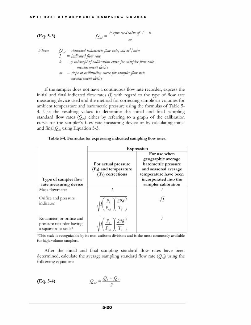
sampling period. If the sampler has a continuous flow rate recorder, determine the average indicated flow rate (I) for the sampling period from the recorder trace. Express I with regard to the type of flow rate measuring device used and the method of correcting sample air volumes for ambient temperature and barometric pressure by using the formulas of Table 5-3. Use the resulting value to determine Qstd, either by referring to a graph of the calibration curve for the sampler flow rate measuring device or by calculating Qstd using the following equation:
A P T I 4 3 5 : A T M O S P H E R I C S A M P L I N G C O U R S E
5-20
(Eq. 5-3) m
bI of value ExpressedQstd
Where: Qstd = standard volumetric flow rate, std m3/min I = indicated flow rate b = y-intercept of calibration curve for sampler flow rate measurement device m = slope of calibration curve for sampler flow rate measurement device
If the sampler does not have a continuous flow rate recorder, express the
initial and final indicated flow rates (I) with regard to the type of flow rate measuring device used and the method for correcting sample air volumes for ambient temperature and barometric pressure using the formulas of Table 5-4. Use the resulting values to determine the initial and final sampling standard flow rates (Qstd) either by referring to a graph of the calibration curve for the sampler’s flow rate measuring device or by calculating initial and final Qstd using Equation 5-3.
Table 5-4. Formulas for expressing indicated sampling flow rates.
Type of sampler flow rate measuring device
Expression
For actual pressure (P3) and temperature
(T3) corrections
For use when geographic average barometric pressure and seasonal average
temperature have been incorporated into the sampler calibration
Mass flowmeter I I
Orifice and pressure indicator
3std
3
T
298
P
PI
I
Rotameter, or orifice and pressure recorder having a square root scale*
3std
3
T
298
P
PI
I
*This scale is recognizable by its non-uniform divisions and is the most commonly available
for high-volume samplers.
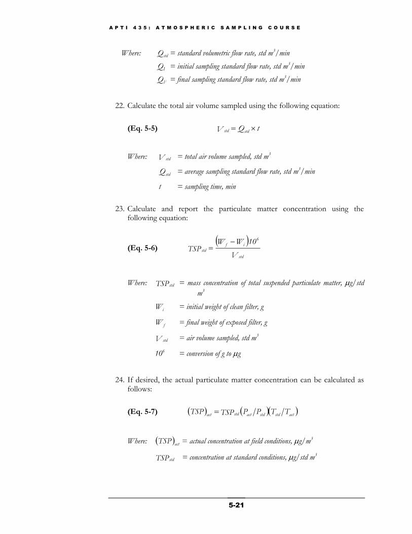
After the initial and final sampling standard flow rates have been determined, calculate the average sampling standard flow rate (Qstd) using the following equation:
(Eq. 5-4) 2
QQQ FI
std
A P T I 4 3 5 : A T M O S P H E R I C S A M P L I N G C O U R S E
5-21
Where: Qstd = standard volumetric flow rate, std m3/min
QI = initial sampling standard flow rate, std m3/min
QF = final sampling standard flow rate, std m3/min
22. Calculate the total air volume sampled using the following equation:
(Eq. 5-5) tQV stdstd
Where: V std = total air volume sampled, std m3
stdQ = average sampling standard flow rate, std m3/min
t = sampling time, min
23. Calculate and report the particulate matter concentration using the
following equation:
(Eq. 5-6)
V
10 WWTSP
std
6
if
std
Where: TSP std = mass concentration of total suspended particulate matter, g/std
m3
iW = initial weight of clean filter, g
fW = final weight of exposed filter, g
V std = air volume sampled, std m3
106 = conversion of g to g
24. If desired, the actual particulate matter concentration can be calculated as follows:
(Eq. 5-7) actstdstdactstdact TTPPTSPTSP
Where: actTSP = actual concentration at field conditions, g/m3
TSP std = concentration at standard conditions, g/std m3
A P T I 4 3 5 : A T M O S P H E R I C S A M P L I N G C O U R S E
5-22
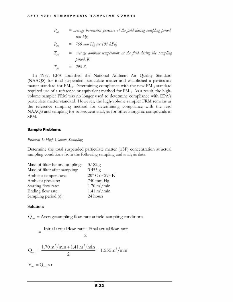
actP = average barometric pressure at the field during sampling period,
mm Hg
stdP = 760 mm Hg (or 101 kPa)
actT = average ambient temperature at the field during the sampling
period, K
stdT = 298 K
In 1987, EPA abolished the National Ambient Air Quality Standard (NAAQS) for total suspended particulate matter and established a particulate matter standard for PM10. Determining compliance with the new PM10 standard required use of a reference or equivalent method for PM10. As a result, the high-volume sampler FRM was no longer used to determine compliance with EPA’s particulate matter standard. However, the high-volume sampler FRM remains as the reference sampling method for determining compliance with the lead NAAQS and sampling for subsequent analysis for other inorganic compounds in SPM.
Sample Problems
Problem 1: High-Volume Sampling
Determine the total suspended particulate matter (TSP) concentration at actual sampling conditions from the following sampling and analysis data. Mass of filter before sampling: 3.182 g Mass of filter after sampling: 3.455 g
Ambient temperature: 20 C or 293 K Ambient pressure: 740 mm Hg Starting flow rate: 1.70 m3/min Ending flow rate: 1.41 m3/min Sampling period (t): 24 hours Solution:
conditionssampling fieldat flow ratesampling AverageQact
= 2
flow rateactual Final flow rateactual Initial
minm 1.5552
minm 41.1minm 70.1Q 3
33
act
tQV actact
A P T I 4 3 5 : A T M O S P H E R I C S A M P L I N G C O U R S E
5-23
33
act m 2.2239hrmin 6024hrminm 1.555V
μg000,273gμg10 g 0.273 g3.182- g3.455collected TSPof Mass 6
TSPact concentration = Mass of TSP/Vact
3
act m 2239.2μg 273,000TSP
3mμg 122ionconcentrat TSP
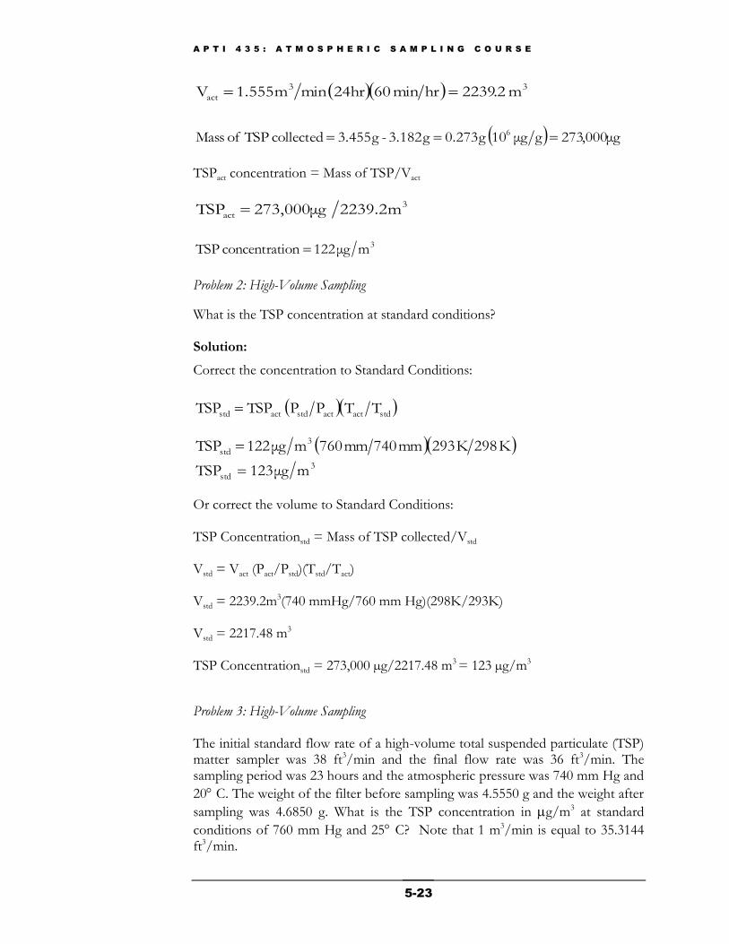
Problem 2: High-Volume Sampling
What is the TSP concentration at standard conditions? Solution:
Correct the concentration to Standard Conditions:
stdactactstdactstd TTPP TSPTSP
K 298K 293mm 740mm 760mμg 122TSP 3
std
3
std mμg 123TSP
Or correct the volume to Standard Conditions: TSP Concentrationstd = Mass of TSP collected/Vstd Vstd = Vact (Pact/Pstd)(Tstd/Tact) Vstd = 2239.2m3(740 mmHg/760 mm Hg)(298K/293K) Vstd = 2217.48 m3
TSP Concentrationstd = 273,000 µg/2217.48 m3 = 123 µg/m3
Problem 3: High-Volume Sampling The initial standard flow rate of a high-volume total suspended particulate (TSP) matter sampler was 38 ft3/min and the final flow rate was 36 ft3/min. The sampling period was 23 hours and the atmospheric pressure was 740 mm Hg and
20 C. The weight of the filter before sampling was 4.5550 g and the weight after
sampling was 4.6850 g. What is the TSP concentration in g/m3 at standard
conditions of 760 mm Hg and 25 C? Note that 1 m3/min is equal to 35.3144 ft3/min.
A P T I 4 3 5 : A T M O S P H E R I C S A M P L I N G C O U R S E
5-24
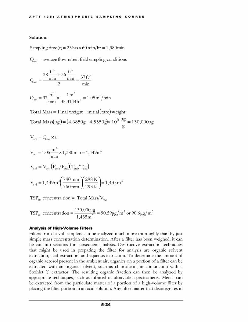
Solution:
min 1,380hrmin 60 hrs 23(t) timeSampling
conditionssampling fieldat flow rate averageQact
min
ft 37
2
min
ft36
min
ft38
Q3
33
act
minm 1.05ft35.3144
m 1
min
ft37Q 3
3
33
act
weight tareinitial weightFinal Total Mass
μg 130,000g
μg6104.5550g4.6850gμgTotal Mass
tQV actact
33
act 1,449mmin 1,380min
m1.05V
actstdstdactactstd TTPP VV
33
std m 1,435K 293
K 298
mm 760
mm 740m 1,449V
stdstd Vs Total Mastionconcentra TSP
33
3std mμg 90.6or mμg 90.59m 1,435
μg 130,000ionconcentrat TSP
Analysis of High-Volume Filters
Filters from hi-vol samplers can be analyzed much more thoroughly than by just simple mass concentration determination. After a filter has been weighed, it can be cut into sections for subsequent analysis. Destructive extraction techniques that might be used in preparing the filter for analysis are organic solvent extraction, acid extraction, and aqueous extraction. To determine the amount of organic aerosol present in the ambient air, organics on a portion of a filter can be extracted with an organic solvent, such as chloroform, in conjunction with a Soxhlet ® extractor. The resulting organic fraction can then be analyzed by appropriate techniques, such as infrared or ultraviolet spectrometry. Metals can be extracted from the particulate matter of a portion of a high-volume filter by placing the filter portion in an acid solution. Any filter matter that disintegrates in
A P T I 4 3 5 : A T M O S P H E R I C S A M P L I N G C O U R S E
5-25
the acid can be removed by centrifugation. After extraction, the resulting soluble metal solution can be analyzed by a number of methods, including atomic absorption spectrophotometry, atomic emission spectroscopy, polarography, and inductively coupled plasma emission spectroscopy. Water-soluble species (such as sulfates and nitrates) of the particulate matter of a high-volume filter can be extracted using deionized, distilled water. The resulting solution can then be analyzed using methods such as ultraviolet or visible spectrometry.
Sometimes it is necessary that the filter remain intact after analysis. Nondestructive analytical techniques, such as neutron activation x-ray fluorescence, and electron or optical microscopy, can be used in these cases.
The above-mentioned analyses are not required for all filters. Therefore, it must be carefully decided what analyses should be performed on individual filters.
Sampling Accuracy and Precision
The limits of accuracy and precision of any sampling method must be understood for proper interpretation of data obtained using that method. Factors influencing the accuracy and precision of high-volume sampling include sampler operating characteristics, accuracy of calibration, filter characteristics, location of sampler, nature and concentration of particulate matter and gases in the air being sampled, and the humidity of the air.
Accuracy
As defined in Section 3 of Appendix A of 40 CFR Part 58, accuracy is the degree of agreement between an observed value and an accepted reference value. It includes a combination of random error (precision) and systematic error (bias) components which are due to sampling and analytical operations. The accuracy of the particulate measurements can be affected by several known inherent sources of error in the sampling of particulate matter. These include airflow variation, air volume measurement, loss of volatiles, artifacts, humidity, filter handling, and non-sampled particulate matter. Airflow Variation The weight of material collected on the filter represents the integrated sum of the product of the instantaneous flow rate times the instantaneous particle concentration. Therefore, dividing this weight by the average flow rate over the sampling period yields the true particulate matter concentration only when the flow rate is constant over the period. The error resulting from a non-constant flow rate depends on the magnitude of the instantaneous changes in the flow rate and in the particulate matter concentration. Normally, such errors are not large, but they can be greatly reduced by equipping the sampler with an automatic flow controlling mechanism that maintains constant flow during the sampling period.
The most popular method of constant flow rate regulation uses a constant temperature thermal anemometer sensor to measure mass flow in the throat of the high-volume sampler’s filter adapter (sampling head). Electronic feedback circuitry adjusts the sampler’s motor speed to maintain a constant mass flow. Since mass flow is controlled, the volumetric flow rate can be maintained at
A P T I 4 3 5 : A T M O S P H E R I C S A M P L I N G C O U R S E
5-26
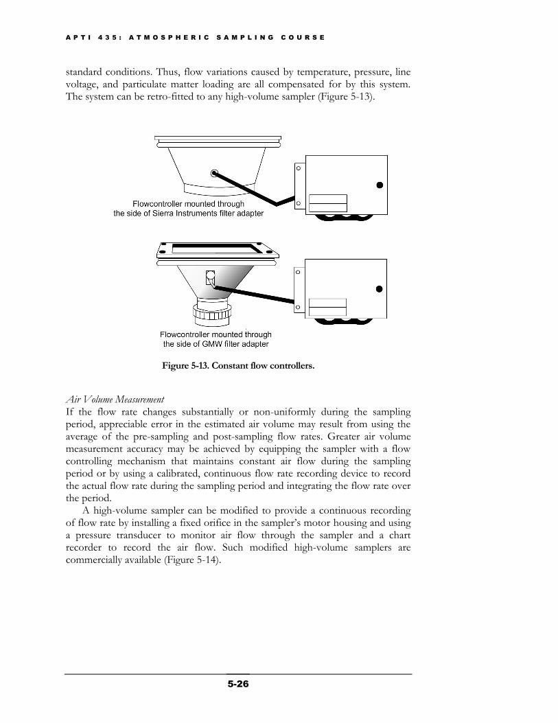
standard conditions. Thus, flow variations caused by temperature, pressure, line voltage, and particulate matter loading are all compensated for by this system. The system can be retro-fitted to any high-volume sampler (Figure 5-13).
Figure 5-13. Constant flow controllers.
Air Volume Measurement If the flow rate changes substantially or non-uniformly during the sampling period, appreciable error in the estimated air volume may result from using the average of the pre-sampling and post-sampling flow rates. Greater air volume measurement accuracy may be achieved by equipping the sampler with a flow controlling mechanism that maintains constant air flow during the sampling period or by using a calibrated, continuous flow rate recording device to record the actual flow rate during the sampling period and integrating the flow rate over the period.
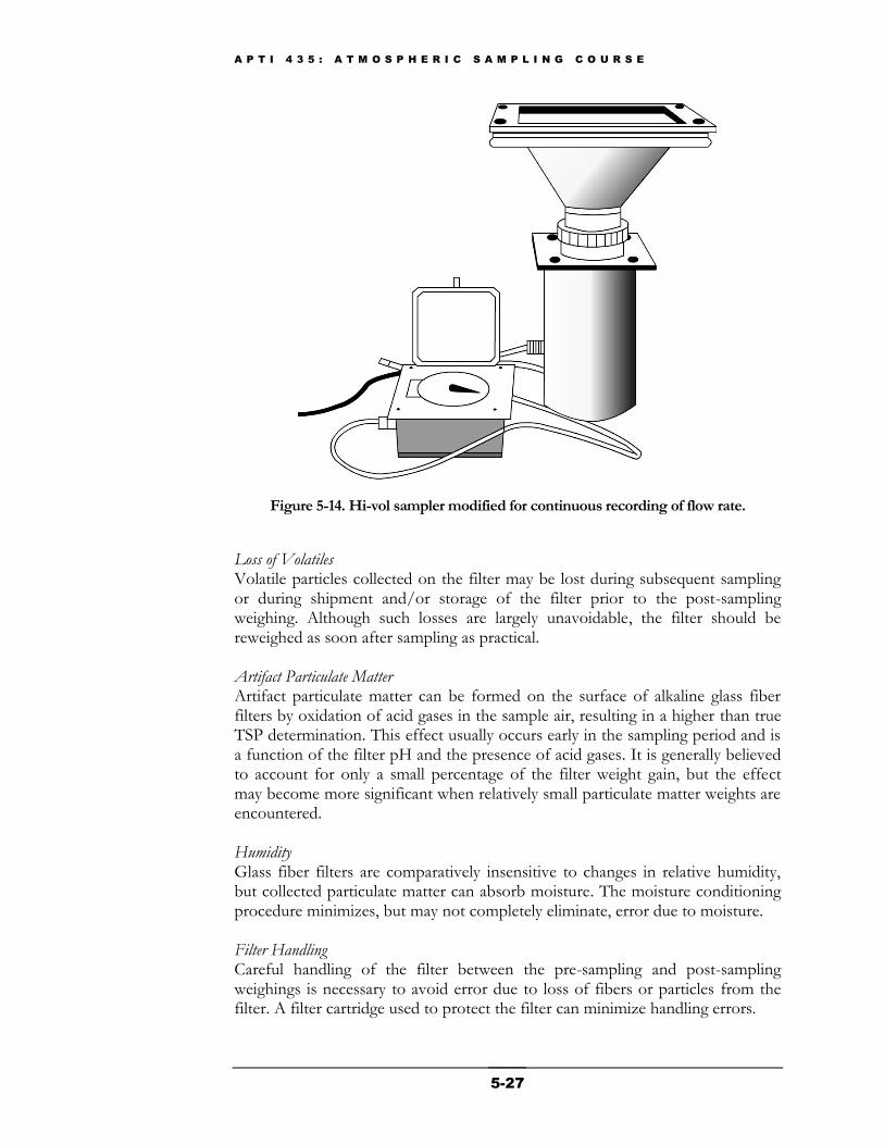
A high-volume sampler can be modified to provide a continuous recording of flow rate by installing a fixed orifice in the sampler’s motor housing and using a pressure transducer to monitor air flow through the sampler and a chart recorder to record the air flow. Such modified high-volume samplers are commercially available (Figure 5-14).
A P T I 4 3 5 : A T M O S P H E R I C S A M P L I N G C O U R S E
5-27
Figure 5-14. Hi-vol sampler modified for continuous recording of flow rate.
Loss of Volatiles Volatile particles collected on the filter may be lost during subsequent sampling or during shipment and/or storage of the filter prior to the post-sampling weighing. Although such losses are largely unavoidable, the filter should be reweighed as soon after sampling as practical. Artifact Particulate Matter Artifact particulate matter can be formed on the surface of alkaline glass fiber filters by oxidation of acid gases in the sample air, resulting in a higher than true TSP determination. This effect usually occurs early in the sampling period and is a function of the filter pH and the presence of acid gases. It is generally believed to account for only a small percentage of the filter weight gain, but the effect may become more significant when relatively small particulate matter weights are encountered. Humidity Glass fiber filters are comparatively insensitive to changes in relative humidity, but collected particulate matter can absorb moisture. The moisture conditioning procedure minimizes, but may not completely eliminate, error due to moisture. Filter Handling Careful handling of the filter between the pre-sampling and post-sampling weighings is necessary to avoid error due to loss of fibers or particles from the filter. A filter cartridge used to protect the filter can minimize handling errors.
A P T I 4 3 5 : A T M O S P H E R I C S A M P L I N G C O U R S E
5-28
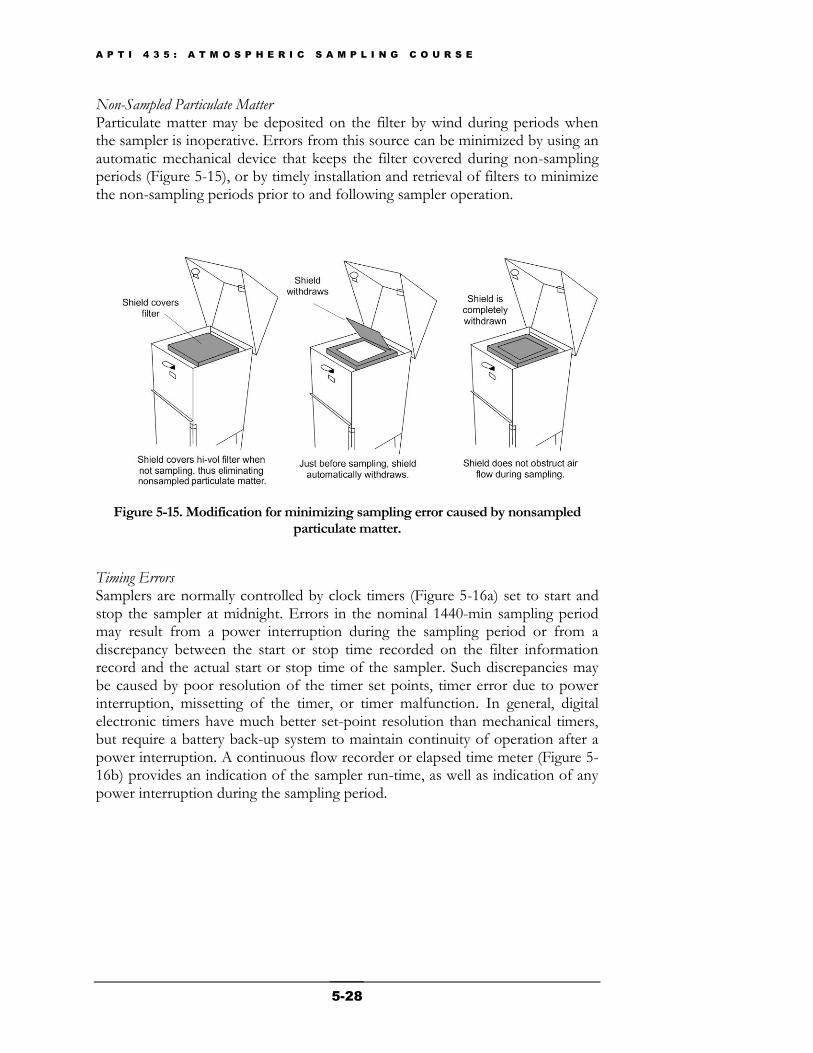
Non-Sampled Particulate Matter Particulate matter may be deposited on the filter by wind during periods when the sampler is inoperative. Errors from this source can be minimized by using an automatic mechanical device that keeps the filter covered during non-sampling periods (Figure 5-15), or by timely installation and retrieval of filters to minimize the non-sampling periods prior to and following sampler operation.
Figure 5-15. Modification for minimizing sampling error caused by nonsampled particulate matter.
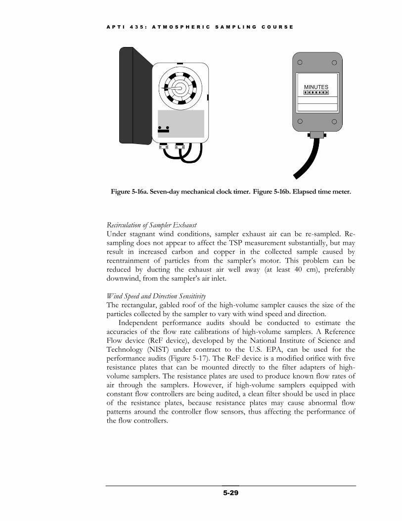
Timing Errors Samplers are normally controlled by clock timers (Figure 5-16a) set to start and stop the sampler at midnight. Errors in the nominal 1440-min sampling period may result from a power interruption during the sampling period or from a discrepancy between the start or stop time recorded on the filter information record and the actual start or stop time of the sampler. Such discrepancies may be caused by poor resolution of the timer set points, timer error due to power interruption, missetting of the timer, or timer malfunction. In general, digital electronic timers have much better set-point resolution than mechanical timers, but require a battery back-up system to maintain continuity of operation after a power interruption. A continuous flow recorder or elapsed time meter (Figure 5-16b) provides an indication of the sampler run-time, as well as indication of any power interruption during the sampling period.
A P T I 4 3 5 : A T M O S P H E R I C S A M P L I N G C O U R S E
5-29
Figure 5-16a. Seven-day mechanical clock timer. Figure 5-16b. Elapsed time meter.
Recirculation of Sampler Exhaust Under stagnant wind conditions, sampler exhaust air can be re-sampled. Re-sampling does not appear to affect the TSP measurement substantially, but may result in increased carbon and copper in the collected sample caused by reentrainment of particles from the sampler’s motor. This problem can be reduced by ducting the exhaust air well away (at least 40 cm), preferably downwind, from the sampler’s air inlet.
Wind Speed and Direction Sensitivity The rectangular, gabled roof of the high-volume sampler causes the size of the particles collected by the sampler to vary with wind speed and direction.
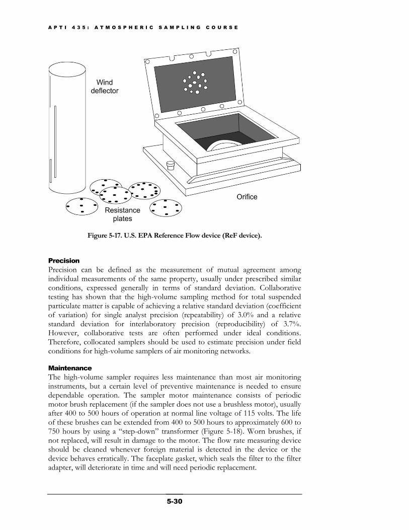
Independent performance audits should be conducted to estimate the accuracies of the flow rate calibrations of high-volume samplers. A Reference Flow device (ReF device), developed by the National Institute of Science and Technology (NIST) under contract to the U.S. EPA, can be used for the performance audits (Figure 5-17). The ReF device is a modified orifice with five resistance plates that can be mounted directly to the filter adapters of high-volume samplers. The resistance plates are used to produce known flow rates of air through the samplers. However, if high-volume samplers equipped with constant flow controllers are being audited, a clean filter should be used in place of the resistance plates, because resistance plates may cause abnormal flow patterns around the controller flow sensors, thus affecting the performance of the flow controllers.
A P T I 4 3 5 : A T M O S P H E R I C S A M P L I N G C O U R S E
5-30
Figure 5-17. U.S. EPA Reference Flow device (ReF device).
Precision
Precision can be defined as the measurement of mutual agreement among individual measurements of the same property, usually under prescribed similar conditions, expressed generally in terms of standard deviation. Collaborative testing has shown that the high-volume sampling method for total suspended particulate matter is capable of achieving a relative standard deviation (coefficient of variation) for single analyst precision (repeatability) of 3.0% and a relative standard deviation for interlaboratory precision (reproducibility) of 3.7%. However, collaborative tests are often performed under ideal conditions. Therefore, collocated samplers should be used to estimate precision under field conditions for high-volume samplers of air monitoring networks.
Maintenance
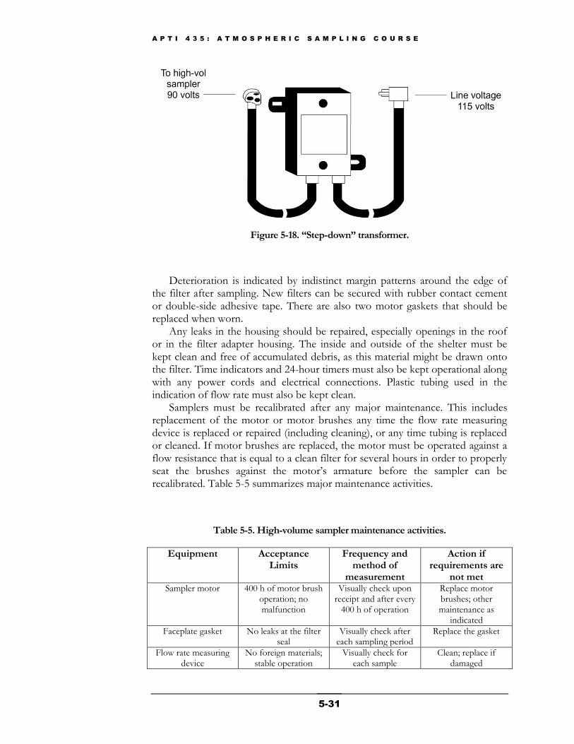
The high-volume sampler requires less maintenance than most air monitoring instruments, but a certain level of preventive maintenance is needed to ensure dependable operation. The sampler motor maintenance consists of periodic motor brush replacement (if the sampler does not use a brushless motor), usually after 400 to 500 hours of operation at normal line voltage of 115 volts. The life of these brushes can be extended from 400 to 500 hours to approximately 600 to 750 hours by using a ―step-down‖ transformer (Figure 5-18). Worn brushes, if not replaced, will result in damage to the motor. The flow rate measuring device should be cleaned whenever foreign material is detected in the device or the device behaves erratically. The faceplate gasket, which seals the filter to the filter adapter, will deteriorate in time and will need periodic replacement.
A P T I 4 3 5 : A T M O S P H E R I C S A M P L I N G C O U R S E
5-31
Figure 5-18. “Step-down” transformer.
Deterioration is indicated by indistinct margin patterns around the edge of the filter after sampling. New filters can be secured with rubber contact cement or double-side adhesive tape. There are also two motor gaskets that should be replaced when worn.
Any leaks in the housing should be repaired, especially openings in the roof or in the filter adapter housing. The inside and outside of the shelter must be kept clean and free of accumulated debris, as this material might be drawn onto the filter. Time indicators and 24-hour timers must also be kept operational along with any power cords and electrical connections. Plastic tubing used in the indication of flow rate must also be kept clean.
Samplers must be recalibrated after any major maintenance. This includes replacement of the motor or motor brushes any time the flow rate measuring device is replaced or repaired (including cleaning), or any time tubing is replaced or cleaned. If motor brushes are replaced, the motor must be operated against a flow resistance that is equal to a clean filter for several hours in order to properly seat the brushes against the motor’s armature before the sampler can be recalibrated. Table 5-5 summarizes major maintenance activities.
Table 5-5. High-volume sampler maintenance activities.
Equipment Acceptance Limits
Frequency and method of
measurement
Action if requirements are
not met Sampler motor 400 h of motor brush
operation; no malfunction
Visually check upon receipt and after every
400 h of operation
Replace motor brushes; other maintenance as
indicated
Faceplate gasket No leaks at the filter seal
Visually check after each sampling period
Replace the gasket
Flow rate measuring device
No foreign materials; stable operation
Visually check for each sample
Clean; replace if damaged
A P T I 4 3 5 : A T M O S P H E R I C S A M P L I N G C O U R S E
5-32
Motor gaskets Leak-free fit Visually check after each 400 h of
operation
Replace gaskets
Filter adapter (sampling head)
No leaks Visually check after each 200 h of
operation
Replace filter adapter
Summary
Although the high-volume method rarely serves the purpose for which it was originally designed (i.e., determining TSP concentration), it continues to be the method of choice for the determination of lead in SPM. Additionally, the high-volume method is increasingly being used to collect a sample for later analysis for metals (i.e. inorganic particles) as interest in assessing air toxics continues to increase.
5.4 FRM for the Determination of Particulate
Matter as PM10
Applicability
The Federal Reference Method (FRM) for PM10 described here is provided from Appendices J and M of 40 CFR Part 50. This method provides for the measurement of the mass concentration of particulate matter with an
aerodynamic diameter less than or equal to a nominal 10 m (PM10) in ambient air over a 24-hour period for purposes of determining attainment and maintenance of the primary and secondary national ambient air quality standards for particulate matter. The measurement process is nondestructive, and the PM10 sample can be subjected to subsequent physical or chemical analyses. Quality assurance procedures and guidance are provided in 40 CFR Part 58, Appendices A and B, and in Volume II of the QA Handbook. Although this section discusses the Federal Reference Method (FRM) for PM10, Class III (continuous monitors) Federal Equivalent Methods (FEM) have been approved by EPA for time-resolved and 24-hour integrated mass concentrations of PM10. These FEM monitors (Beta Gauge and TEOM®) are discussed in the ―Continuous Monitoring for Particulate Matter‖ section of this chapter.
Principle
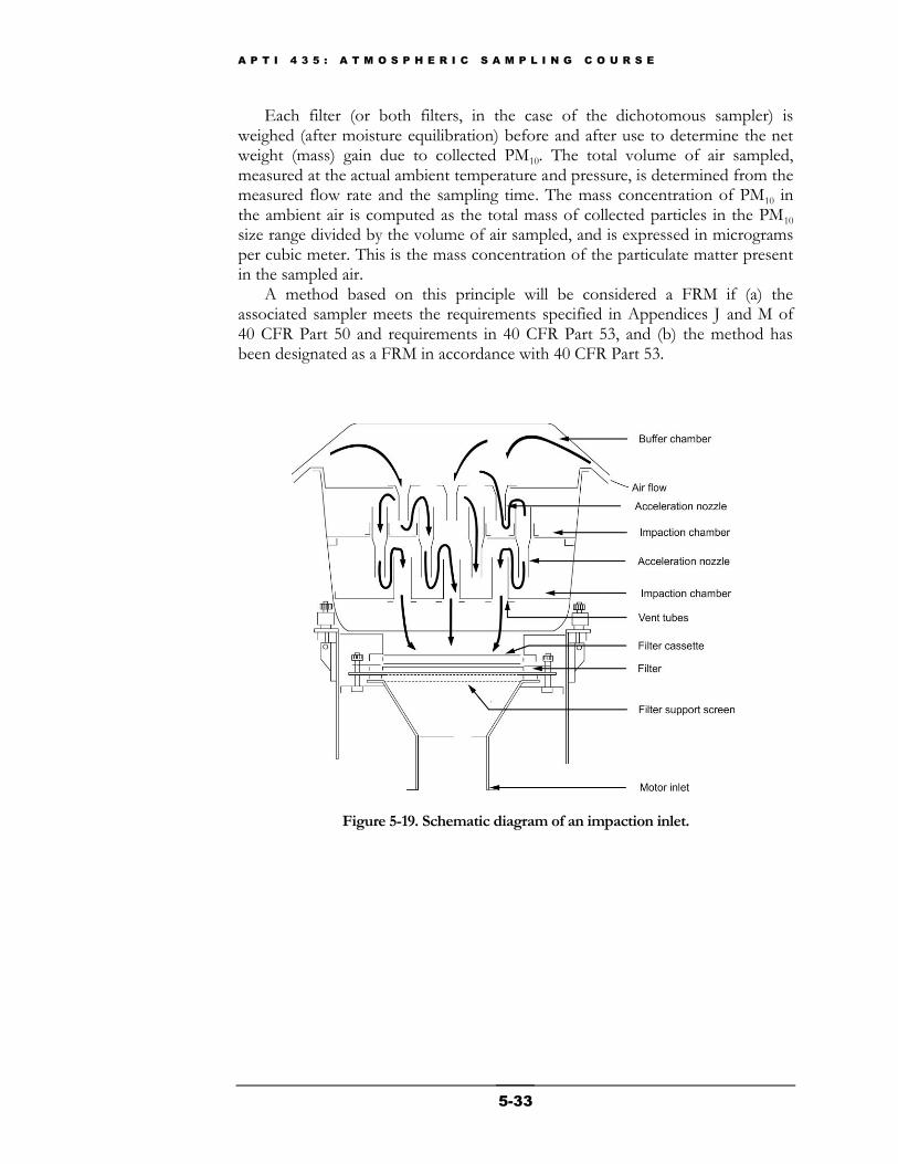
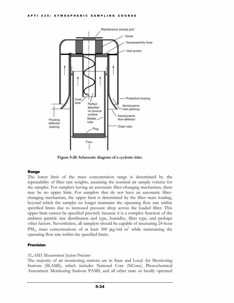
In the FRM for PM10, an air sampler draws ambient air at a constant flow rate into a specially shaped inlet where the suspended particulate matter is inertially separated into one or more size fractions within the PM10 size range (Figures 5-19 and 5-20). Each size fraction in the PM10 size range is then collected on a separate filter over the specified sampling period. The particle size discrimination characteristics (sampling effectiveness and 50% cutpoint) of the sampler inlet are prescribed as performance specifications in 40 CFR Part 53. Two types of samplers that meet EPA FRM designation for PM10 requirements are the high-volume (1000 L/min) PM10 sampler and the dichotomous sampler (16.7 L/min).
A P T I 4 3 5 : A T M O S P H E R I C S A M P L I N G C O U R S E
5-33
Each filter (or both filters, in the case of the dichotomous sampler) is weighed (after moisture equilibration) before and after use to determine the net weight (mass) gain due to collected PM10. The total volume of air sampled, measured at the actual ambient temperature and pressure, is determined from the measured flow rate and the sampling time. The mass concentration of PM10 in the ambient air is computed as the total mass of collected particles in the PM10 size range divided by the volume of air sampled, and is expressed in micrograms per cubic meter. This is the mass concentration of the particulate matter present in the sampled air.
A method based on this principle will be considered a FRM if (a) the associated sampler meets the requirements specified in Appendices J and M of 40 CFR Part 50 and requirements in 40 CFR Part 53, and (b) the method has been designated as a FRM in accordance with 40 CFR Part 53.
Figure 5-19. Schematic diagram of an impaction inlet.
A P T I 4 3 5 : A T M O S P H E R I C S A M P L I N G C O U R S E
5-34
Figure 5-20. Schematic diagram of a cyclonic inlet.
Range
The lower limit of the mass concentration range is determined by the repeatability of filter tare weights, assuming the nominal air sample volume for the sampler. For samplers having an automatic filter-changing mechanism, there may be no upper limit. For samplers that do not have an automatic filter-changing mechanism, the upper limit is determined by the filter mass loading, beyond which the sampler no longer maintains the operating flow rate within specified limits due to increased pressure drop across the loaded filter. This upper limit cannot be specified precisely because it is a complex function of the ambient particle size distribution and type, humidity, filter type, and perhaps other factors. Nevertheless, all samplers should be capable of measuring 24-hour
PM10 mass concentrations of at least 300 g/std m3 while maintaining the operating flow rate within the specified limits.
Precision
SLAMS Measurement System Precision The majority of air monitoring stations are in State and Local Air Monitoring Stations (SLAMS), which includes National Core (NCore), Photochemical Assessment Monitoring Stations PAMS, and all other state or locally operated
A P T I 4 3 5 : A T M O S P H E R I C S A M P L I N G C O U R S E
5-35
stations that have not been designated as Special Purpose Monitoring (SPM) or Prevention of Significant Deterioration (PSD) sites. Appendix A of 40 CFR Part 58 addresses the QA/QC requirements applicable to SLAMS, SPM, and PSD sites.
Appendix A of 40 CFR Part 58 states that all ambient monitoring methods or analyzers used in SLAMS shall be tested periodically to quantitatively assess the quality of the SLAMS data. The terminology used to define the quality or uncertainty of the SLAMS measurements includes precision, accuracy, and bias. Precision is defined as the measurement of mutual agreement among individual measurements of the same property, usually under prescribed similar conditions, expressed generally in terms of the standard deviation. The SLAMS precision
goal for PM10 is 15% (QA Handbook, Volume II, Section 2.011). Estimates of the precision of SLAMS automated methods for PM10 are made
based on checks of the operational flow rate of each analyzer using a flow rate transfer standard. These checks must be conducted at least once every 2 weeks. For networks using manual methods for PM10, precision is determined using collocated samplers at selected sites. One of the samplers is designated as the primary sampler whose data will be used to report air quality for the site, and the other sampler is designated as the duplicate sampler. Estimates of the precision are calculated according to the procedures specified in Section 4 of Appendix A of Part 58. Initial Operational Precision of a FRM Sampler In addition to the Part 58 precision requirements associated with SLAMS PM10 measurements, there are specifications in Appendix J of 40 CFR Part 50 which address the initial operational precision of a candidate FRM sampler. These
specifications state that the precision of PM10 samplers must be 5 g/m3 for
PM10 concentrations below 80 g/m3, and 7% for PM10 concentrations above 80
g/m3. The detailed and lengthy tests to determine whether or not a candidate sampler complies with the precision specifications are included in 40 CFR Part 53, as are the provisions for EPA designation of reference (FRM) and equivalent (FEM) methods for candidate PM10 monitors.
Accuracy
SLAMS Measurement System Accuracy Appendix A of Part 58 defines accuracy as the degree of agreement between an observed value and an acceptable reference value. Accuracy includes a combination of random error (precision) and systematic error (bias) components which are due to sampling and analytical operations. The accuracy goal for
SLAMS PM10 measurements is 20% (QA Handbook, Volume II, Section 3.01). The accuracy of automated PM10 analyzers is determined by conducting quarterly audits of at least 25% of the SLAMS analyzers so that each analyzer is audited at least once per year. The audit is performed by measuring the analyzer’s normal operating flow rate, using a certified flow rate transfer standard. The percent difference between the sampler’s indicated flow rate and the transfer standard
A P T I 4 3 5 : A T M O S P H E R I C S A M P L I N G C O U R S E
5-36
flow rate is used to calculate accuracy. The procedures are specified in Appendix A of Part 58. Initial Operational Accuracy of a FRM Sampler It is difficult to define the absolute accuracy of PM10 samplers because of the variation in the size of atmospheric particles and the variation in concentration with particle size. Therefore, 40 CFR Part 53 includes the specification for the sampling effectiveness of PM10 samplers that are candidates for reference (FRM) or equivalent method (FEM) designation. This specification requires that the expected mass concentration calculated for a candidate PM10 sampler, when
sampling a specified particle size distribution, be within 10% of that calculated for an ideal sampler whose sampling effectiveness is explicitly specified. In
addition, the particle size for 50% sampling effectiveness is required to be 10
0.5 m. Other accuracy specifications prescribed for reference (FRM) or equivalent method (FEM) designation are related to flow measurement and calibration, filter media, analytical weighing procedures, and artifacts.
Potential Sources of Error
There are a number of possible sources of error in measuring PM10 concentration levels in ambient air, including volatile particles, artifacts, humidity, filter handling, flow rate variation, and air volume determination. The FRM also addresses the configuration of the sampler, filter calibration, operational procedure, and concentration calculation. Volatile Particles Volatile particles collected on filters are often lost during shipment and/or storage of the filters prior to the postsampling weighing. Although shipment or storage of loaded filters is sometimes unavoidable, filters should be reweighed as soon as practical to minimize these losses. Filters are usually stored and shipped cold in order to prevent volatile losses. Artifacts Positive artifacts in PM10 concentration measurements can result from absorption or adsorption on filters and collected PM. Common positive artifacts are sulfur dioxide, nitric acid, and organic carbon species. Positive artifacts not only overestimate true PM mass, but they can also change the filter alkalinity. For example, retention of sulfur dioxide on filters, followed by oxidation to sulfate (sulfate formation), is a phenomenon that increases with increasing filter alkalinity. Little or no artifact sulfate formation should occur using filters that meet the alkalinity specification in the FRM in Appendix M of 40 CFR Part 50. Artifact nitrate formation, resulting primarily from retention of nitric acid, occurs to varying degrees on many filter types, including glass fiber, cellulose ester, and many quartz fiber filters. Loss of true atmospheric particulate nitrate during or following sampling may also occur due to dissociation or chemical reaction. This
phenomenon has been observed on Teflon
filters and inferred for quartz fiber filters. The magnitude of nitrate artifact errors in PM10 mass concentration measurements will vary with location and ambient temperature; however, for
A P T I 4 3 5 : A T M O S P H E R I C S A M P L I N G C O U R S E
5-37
most sampling locations, these errors are expected to be small. Glass and quartz fiber filters are especially prone to the adsorption of organic carbonaceous species in the air. Denuders can be used to selectively remove gaseous components of ambient air drawn into the sampler so that only particles are collected on the filter.
A negative artifact occurs when chemical components of PM are lost. Changes in ambient concentrations of gas and particle phase organic components, and in temperature, can alter volatile and semi-volatile species adsorbed onto collected particles. Volatile and semi-volatile components of PM can be lost during temperature increases during sampling and transport, and when sampling at high face velocities. For this reason, PM10 filters should be transported cold. The negative artifact associated with filter velocity is considered negligible under typical PM10 and PM2.5 flow rates. The negative bias related to negative artifacts is typically much less than the bias of positive artifacts for typical ambient conditions, sampling face velocities, and collection times. Humidity The effects of ambient humidity on the sample are unavoidable. The filter equilibration procedure in the FRM is designed to minimize the effects of moisture on the filter medium. For this reason, Teflon filters are pre-weighed and post-weighed at controlled temperature and humidity. Filter Handling Careful handling of filters between presampling and postsampling weighings is necessary to avoid errors due to damaged filters or loss of collected particles from the filters. Use of a filter cartridge or cassette may reduce the magnitude of these errors. Flow Rate Variation Variations in the sampler’s operating flow rate may alter the particle size discrimination characteristics of the sampler inlet. The magnitude of this error will depend on the sensitivity of the inlet to variations in flow rate and on the particle distribution in the atmosphere during the sampling period. The use of a flow control device is required to minimize this error. Air Volume Determination Errors in the air volume determination may result from errors in the flow rate and/or sampling time measurements. The flow control device serves to minimize errors in the flow rate determination, and an elapsed time meter is required to minimize the error in the sampling time measurement.
PM10
Sampler Apparatus
The sampler is designed to:
draw the air sample into the sampler inlet and through the particle collection filter at a uniform face velocity,
hold and seal the filter in a horizontal position so that sample air is drawn downward through the filter,
A P T I 4 3 5 : A T M O S P H E R I C S A M P L I N G C O U R S E
5-38
allow the filter to be installed and removed conveniently,
protect the filter and sampler from precipitation and prevent insects and other debris from being sampled,
minimize air leaks that would cause error in the measurement of the air volume passing through the filter,
discharge exhaust air at a sufficient distance from the sampler inlet to minimize the sampling of exhaust air, and
minimize the collection of dust from the supporting surface.
Filter Media
No commercially available filter medium is ideal in all respects for all PM10 samplers. In addition to the user's goal of determining concentration, other factors such as cost, ease of handling, and physical and chemical characteristics all contribute to the specific filter chosen for sampling. In addition to those factors, certain types of filters may not be suitable for use with some samplers, particularly under heavy loading conditions (high mass concentrations), because of high or rapid increase in the filter flow resistance that would exceed the capability of the sampler’s flow control device. However, samplers equipped with automatic filter-changing mechanisms may allow the use of these types of filters.
Filter specifications are provided in the FRM and address collection efficiency, integrity, and alkalinity. The filter medium collection efficiency must be greater than 99% as measured by the dioctyl phthalate (DOP) test, American Society of Testing Materials (ASTM) 2986.
The filter conditioning environment must control the temperature to 3C
and the relative humidity to 5%. Other topics covered in the FRM include the analytical balance calibration procedure, sampler operational procedure, and sample maintenance.
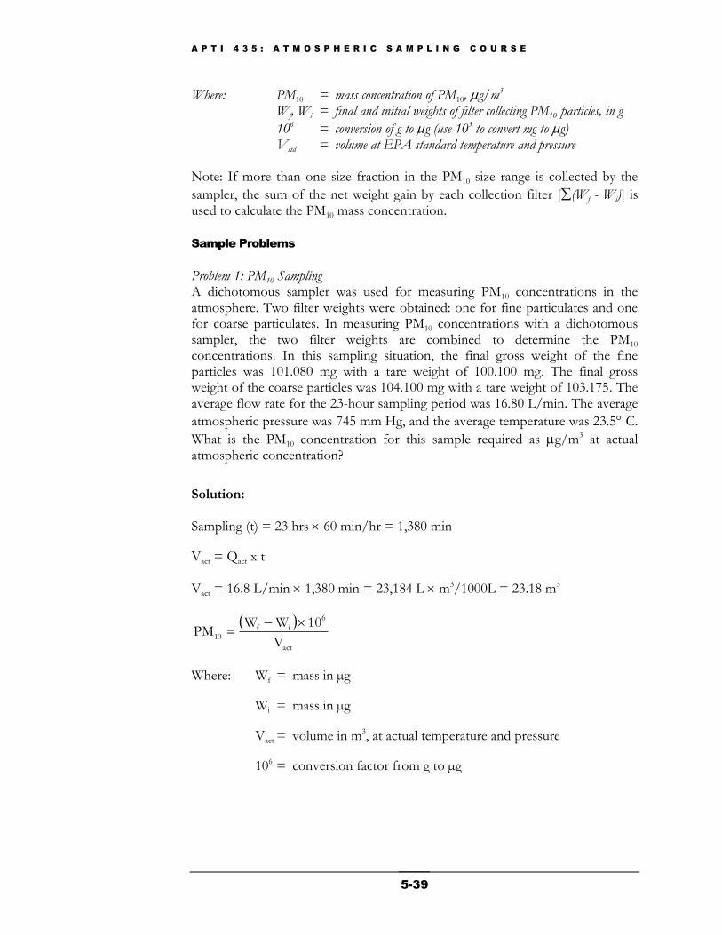
Calculations
Calculate the total volume of air sampled as: (Eq. 5-8) Vact = Qat Where: Vact = total air sampled at ambient temperature and pressure, m3
Qa = average sample flow rate at ambient temperature and pressure, m3/min
t = sampling time, min
Calculate the PM10 concentration as:
(Eq. 5-9)
std
6
if
10V
x10WWPM
A P T I 4 3 5 : A T M O S P H E R I C S A M P L I N G C O U R S E
5-39
Where: PM10 = mass concentration of PM10, g/m3 Wf, Wi = final and initial weights of filter collecting PM10
particles, in g
106 = conversion of g to g (use 103 to convert mg to g) Vstd = volume at EPA standard temperature and pressure Note: If more than one size fraction in the PM10 size range is collected by the
sampler, the sum of the net weight gain by each collection filter [(Wf - Wi)] is used to calculate the PM10 mass concentration.
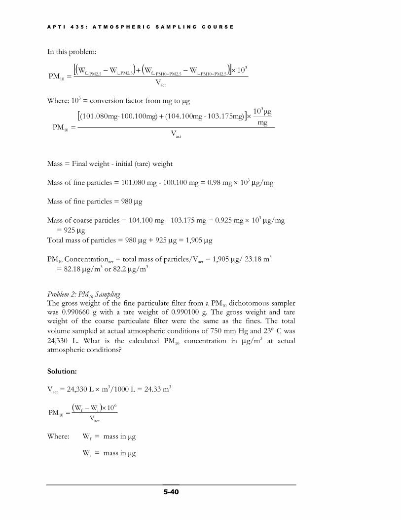
Sample Problems
Problem 1: PM10 Sampling A dichotomous sampler was used for measuring PM10 concentrations in the atmosphere. Two filter weights were obtained: one for fine particulates and one for coarse particulates. In measuring PM10 concentrations with a dichotomous sampler, the two filter weights are combined to determine the PM10 concentrations. In this sampling situation, the final gross weight of the fine particles was 101.080 mg with a tare weight of 100.100 mg. The final gross weight of the coarse particles was 104.100 mg with a tare weight of 103.175. The average flow rate for the 23-hour sampling period was 16.80 L/min. The average
atmospheric pressure was 745 mm Hg, and the average temperature was 23.5 C.
What is the PM10 concentration for this sample required as g/m3 at actual atmospheric concentration?
Solution:
Sampling (t) = 23 hrs 60 min/hr = 1,380 min
Vact = Qact x t
Vact = 16.8 L/min 1,380 min = 23,184 L m3/1000L = 23.18 m3
act
6
if10
V
10WWPM
Where: Wf = mass in µg
Wi = mass in µg
Vact = volume in m3, at actual temperature and pressure
106 = conversion factor from g to µg
A P T I 4 3 5 : A T M O S P H E R I C S A M P L I N G C O U R S E
5-40
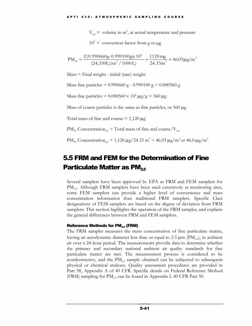
In this problem:
act
3
PM2.5PM10i_PM2.5PM10f_i_PM2.5PM2.5f_
10V
10WWWWPM
Where: 103 = conversion factor from mg to µg
Mass = Final weight - initial (tare) weight
Mass of fine particles = 101.080 mg - 100.100 mg = 0.98 mg 103 g/mg
Mass of fine particles = 980 g
Mass of coarse particles = 104.100 mg - 103.175 mg = 0.925 mg 103 g/mg
= 925 g
Total mass of particles = 980 g + 925 g = 1,905 g
PM10 Concentrationact = total mass of particles/Vact = 1,905 g/ 23.18 m3
= 82.18 g/m3 or 82.2 g/m3
Problem 2: PM10 Sampling The gross weight of the fine particulate filter from a PM10 dichotomous sampler was 0.990660 g with a tare weight of 0.990100 g. The gross weight and tare weight of the coarse particulate filter were the same as the fines. The total
volume sampled at actual atmospheric conditions of 750 mm Hg and 23 C was
24,330 L. What is the calculated PM10 concentration in g/m3 at actual atmospheric conditions?
Solution:
Vact = 24,330 L m3/1000 L = 24.33 m3
act
6if
10V
10WWPM
Where: Wf = mass in µg
Wi = mass in µg
act
3
10V
mg
μg10 mg) 103.175 -mg (104.100 mg) 100.100-(101.080mg
PM
A P T I 4 3 5 : A T M O S P H E R I C S A M P L I N G C O U R S E
5-41
Vact = volume in m3, at actual temperature and pressure
106 = conversion factor from g to µg
Mass = Final weight - initial (tare) weight
Mass fine particles = 0.990660 g - 0.990100 g = 0.000560 g
Mass fine particles = 0.000560 106 g/g = 560 g
Mass of coarse particles is the same as fine particles, or 560 g
Total mass of fine and coarse = 1,120 g
PM10 Concentrationact = Total mass of fine and coarse/Vact
PM10 Concentrationact = 1,120 g/24.33 m3 = 46.03 g/m3 or 46.0 g/m3
5.5 FRM and FEM for the Determination of Fine
Particulate Matter as PM2.5
Several samplers have been approved by EPA as FRM and FEM samplers for PM2.5. Although FRM samplers have been used extensively at monitoring sites, some FEM samplers can provide a higher level of convenience and mass concentration information than traditional FRM samplers. Specific Class designations of FEM samplers are based on the degree of deviation from FRM samplers. This section highlights the operation of the FRM sampler, and explains the general differences between FRM and FEM samplers.
Reference Methods for PM2.5
(FRM)
The FRM sampler measures the mass concentration of fine particulate matter,
having an aerodynamic diameter less than or equal to 2.5 m (PM2.5), in ambient air over a 24-hour period. The measurements provide data to determine whether the primary and secondary national ambient air quality standards for fine particulate matter are met. The measurement process is considered to be nondestructive, and the PM2.5 sample obtained can be subjected to subsequent physical or chemical analyses. Quality assessment procedures are provided in Part 58, Appendix A of 40 CFR. Specific details on Federal Reference Method (FRM) sampling for PM2.5 can be found in Appendix L 40 CFR Part 50.
3
33
6
10 g/m 03.46m 24.33
mg 1120
L) 1000 / L)(m (24,330
10 x 0.990100g) - (0.990660g 2PM
A P T I 4 3 5 : A T M O S P H E R I C S A M P L I N G C O U R S E
5-42
Principle An electrically powered air sampler draws a 24-hour ambient air sample at a constant volumetric flow rate into a specially shaped inlet (Figure 5-21) and through an inertial particle size separator (WINS Impactor or Very Sharp Cut Cyclone). The suspended particulate matter in the PM2.5 size range is separated from the larger particles (Figure 5-22) and then collected on a polytetrafluoroethylene (PTFE) filter. Each filter is weighed (after moisture and temperature conditioning) before and after sample collection to determine the net gain in weight of PM2.5. The total volume of air sampled at actual temperature and pressure conditions is calculated from the measured flow rate and sampling time. The mass concentration of PM2.5 collected, in micrograms per
cubic meter (g/m3), is calculated by dividing the net gain in weight by the total volume of air sampled. Measurement Range Lower Concentration Limit. The lower detection limit of the mass concentration
measurement range is estimated to be approximately 2 g/m3, based on noted mass changes in field blanks in conjunction with the 24 m3 nominal total air sample volume specified for the 24-hour sample.
Upper Concentration Limit. The upper limit of the mass concentration range is determined by the filter mass loading, beyond which the sampler can no longer maintain the operating flow rate within specified limits (10% of 16.67 L) due to increased pressure drop across the loaded filter. This upper limit cannot be specified precisely because it is a complex function of the ambient particle size distribution and type, humidity, the individual filter used, the capacity of the sampler flow rate control system, and perhaps other factors. Nevertheless, all samplers are estimated to be
capable of measuring 24-hour PM2.5 mass concentrations of at least 200 g/m3 while maintaining the operating flow rate within the specified limits. Sample Period. The required sample period for PM2.5 concentration measurements by this method is 1380 to 1500 minutes (23 to 25 hours). Precision SLAMS Measurement System Precision. As stated in Appendix A of 40 CFR 58, precision is defined as the measurement of mutual agreement among individual measurements of the same property, usually under prescribed similar conditions, expressed generally in terms of the standard deviation. A data quality objective of 10% coefficient of variation (CV) or better has been established for the SLAMS operational precision of PM2.5 monitoring data. Precision Measurements Using Collocated Procedures for Automated and Manual Methods of PM2.5. Appendix A of 40 CFR 58 describes the requirements for measuring the precision of automated and manual methods for PM2.5 using collocated samplers. The requirements include: (1) SLAMS operators
A P T I 4 3 5 : A T M O S P H E R I C S A M P L I N G C O U R S E
5-43
must report the number or percent of collocated samplers per reporting organization, (2) an EPA FRM must be collocated with a monitor having the same EPA FRM designation, (3) for monitors designated as an EPA FEM, 50% of the designated monitors shall be collocated with a monitor having the same designation and 50% shall be collocated with an FRM monitor, and (4) during the initial deployment of the SLAMS network, collocated sites should be in areas likely to be in violation of the NAAQS.
For each pair of collocated samplers at the selected sites, one of the samplers is designated as the primary sampler for the site, and the other sampler is designated as the duplicate sampler. The duplicate sampler must be operated concurrently with the primary sampler and on a one-in-six day sampling schedule. Estimates of the precision are calculated using the procedures specified in Appendix A of Part 58.
Initial Operational Precision of a FRM Sampler. In addition to the requirements associated with SLAMS PM2.5 precision measurements, there are tests in Section 53.58 of 40 CFR Part 53 which are intended to determine the operational precision of candidate PM2.5 samplers during a minimum of 10 days of field operation using three collocated test samplers. In this section, precision is defined as the standard deviation or relative standard deviation of a set of PM2.5
measurements obtained concurrently with three or more collocated samplers in actual ambient air field operation. Calculations to determine whether or not the candidate method passes the precision test are specified. Accuracy and Bias SLAMS Measurement System Accuracy and Bias. Appendix A of Part 58 defines accuracy as the degree of agreement between an observed value and an acceptable reference value. Accuracy includes a combination of random error (precision) and systematic error (bias) components that are due to sampling and analytical operations. An accuracy goal for the PM2.5 sampler’s flow rate has been specified in Section 2.12 of the QA Handbook, Vol. II, Part II. The goal for
accuracy of the sampler flow rate is to be within 2% of the value indicated by
the audit device (during multipoint verification/calibration), or 4% (during
one-point verification checks and audits), and to be within 2% of the sampler’s design flow rate of 16.67 L/min (40 CFR Part 50, Appendix L). Automated Flow Check Accuracy. Flow rate accuracy in SLAMS automated methods (FEM) for PM2.5 is based on checks of the operational flow rate of each analyzer using a certified flow rate transfer standard. These checks must be conducted at least once every 2 weeks, and a randomization with respect to time of day, day of week, and routine service and adjustments is encouraged. An alternative procedure that does not use an external flow rate transfer standard is permissible to obtain the flow rate data from the analyzer’s internal flow meter. This alternative procedure is allowed if several conditions are met, one of which requires the flow meter to be audited with an external flow rate transfer standard at least every six months. Details on both procedures can be found in Appendix
A P T I 4 3 5 : A T M O S P H E R I C S A M P L I N G C O U R S E
5-44
A of 40 CFR Part 58. For either procedure, the difference between the flow rate transfer standard and the indicated flow rate of the sampler is used to assess the accuracy of the flow rate using the calculation procedures contained in 40 CFR Part 58, Appendix A. Manual Flow Check Accuracy. For networks using manual sampling methods for PM2.5, the accuracy of the sampler’s flow rate is determined by auditing the flow rate of each SLAMS sampler each calendar quarter. A certified flow rate transfer standard is used for the audit. The audit flow rate and the indicated flow rate of the sampler are reported and the difference between the two is used to calculate the flow rate accuracy. Like automated methods, a flow rate audit must be performed every six months by a trained experienced technician other than the routine site operator. Additional information on flow check requirements of manual FRM methods can be found in 40 CFR Part 58, Appendix A. Initial Operational Accuracy of a FRM Sampler. It is difficult to define the absolute accuracy of PM2.5 samplers because of the variation in the size of atmospheric particles and the variation in concentration with particle size. Therefore, 40 CFR Part 53 includes the specification for the sampling effectiveness of PM2.5 samplers that are candidates for reference or equivalent method designation. Other specifications for reference or equivalent method designation related to accuracy apply to flow measurement and calibration, filter media, analytical weighing procedures, and artifacts. Measurement System Bias. Bias is defined as the systematic or persistent distortion of a measurement process that causes errors in one direction. The
measurement system bias goal is to be within 10% of the measurement obtained by an independent sampler audit. The sampler bias is assessed from the results of an independent FRM performance evaluation to be administered through the EPA Regional Offices. More details on these requirements are contained in the QA Handbook, Vol. II, Part II, Section 2.12, Subsection 13.3. Filter for PM2.5 Sample Collection
The filters specified in the FRM for PM2.5 are 46.2 mm diameter filters of
polytetrafluoroethylene (PTFE Teflon
), with an integral support ring made of polymethylpentene (PMP) or equivalent inert material. In addition to the type of filter material and support ring, the method includes other filter specifications such as pore size, filter thickness, maximum pressure drop, and filter weight stability.
Although not required for determination of PM2.5 mass concentration under this FRM, additional specifications for the filter must be developed by users who intend to subject PM2.5 filter samples to subsequent chemical analysis. These supplemental specifications include background chemical contamination of the filter and any other filter parameters that may be required by the method of chemical analysis. All such supplemental filter specifications must be compatible with and secondary to the primary filter specifications.
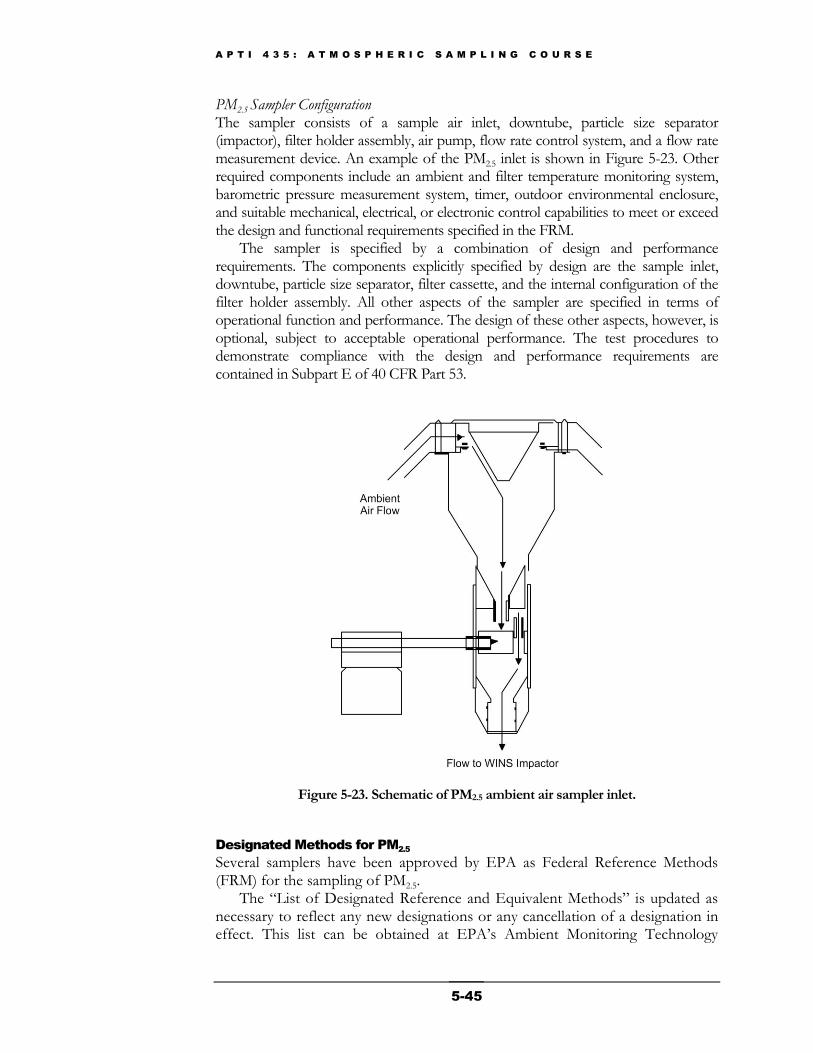
A P T I 4 3 5 : A T M O S P H E R I C S A M P L I N G C O U R S E
5-45
PM2.5 Sampler Configuration
The sampler consists of a sample air inlet, downtube, particle size separator (impactor), filter holder assembly, air pump, flow rate control system, and a flow rate measurement device. An example of the PM2.5 inlet is shown in Figure 5-23. Other required components include an ambient and filter temperature monitoring system, barometric pressure measurement system, timer, outdoor environmental enclosure, and suitable mechanical, electrical, or electronic control capabilities to meet or exceed the design and functional requirements specified in the FRM.
The sampler is specified by a combination of design and performance requirements. The components explicitly specified by design are the sample inlet, downtube, particle size separator, filter cassette, and the internal configuration of the filter holder assembly. All other aspects of the sampler are specified in terms of operational function and performance. The design of these other aspects, however, is optional, subject to acceptable operational performance. The test procedures to demonstrate compliance with the design and performance requirements are contained in Subpart E of 40 CFR Part 53.
Figure 5-23. Schematic of PM2.5 ambient air sampler inlet.
Designated Methods for PM2.5
Several samplers have been approved by EPA as Federal Reference Methods (FRM) for the sampling of PM2.5.
The ―List of Designated Reference and Equivalent Methods‖ is updated as necessary to reflect any new designations or any cancellation of a designation in effect. This list can be obtained at EPA’s Ambient Monitoring Technology
A P T I 4 3 5 : A T M O S P H E R I C S A M P L I N G C O U R S E
5-46
Information (AMTIC) webpage (http://www.epa.gov/ttn/amtic) or at http://www.epa.gov/ttn/amtic/files/ambient/criteria/reference-equivalent-methods-list.pdf.
Equivalent Methods for PM2.5
(FEM)
Equivalent methods for PM2.5 have a much wider latitude in their design, configuration, and operating principle than FRMs. These methods are not required to be based on filter collection of PM2.5; therefore, continuous or semicontinuous analyzers and new types of PM2.5 measurement technologies are not precluded as possible equivalent methods. Equivalent methods are not necessarily required to meet all the requirements specified for FRMs, but they must demonstrate both comparability to FRM measurements and similar PM2.5 measurement precision.
The requirements that some (but not all) candidate methods must meet for designation as equivalent methods by EPA are specified in 40 CFR Part 53. Three classes of equivalent methods have been established in the 40 CFR Part 53 regulations, based on the degree to which a candidate method deviates from the FRM requirements. All three classes of equivalent methods are acceptable for SLAMS or SLAMS-related PM2.5 monitoring. However, not all types of equivalent methods may be equally suited to specific PM2.5 monitoring requirements or applications.
A Class I equivalent method means an equivalent method for PM2.5 or PM10−2.5 which is based on a sampler that is very similar to the sampler specified for reference methods in Appendix L or Appendix O (as applicable) of 40 CFR Part 50, with only minor deviations or modifications, as determined by EPA. For PM2.5, Class I equivalent methods are based on samplers that have minor deviations from the specifications for FRM samplers. However, they must meet the 40 CFR Part 53 tests and other requirements that are applicable to FRM samplers. Also, they must be tested to make sure that the modifications of the candidate Class I equivalent method sampler do not significantly compromise sampler performance. Finally, they must be tested for possible loss of PM2.5 in any new or modified components in the sampler inlet upstream of the sampler filter.
A Class II equivalent method means an equivalent method for PM2.5 or PM10−2.5 that utilizes a PM2.5 sampler or PM10−2.5 sampler in which integrated PM2.5 samples or PM10−2.5 samples are obtained from the atmosphere by filtration and subjected to a subsequent filter conditioning process followed by a gravimetric mass determination. However, this method is not a Class I equivalent method because of substantial deviations from the design specifications of the sampler specified for reference methods in Appendix L or Appendix O (as applicable) of 40 CFR Part 50. Basically, Class II equivalent method samplers are filter-collection based methods that will generally have one or more substantial deviations from the design or performance specification of the FRM. For example, they might have a different inlet, particle size separator, volumetric flow rate, filter, or filter face velocity than a FRM sampler. Consequently, more extensive performance testing is required for designation of Class II equivalent methods. For PM2.5 and PM10-2.5, the procedures for testing physical (design) and performance characteristics of reference methods and Class I and Class II
A P T I 4 3 5 : A T M O S P H E R I C S A M P L I N G C O U R S E
5-47
equivalent methods can be found in Subpart E of 40 CFR Part 53. Additional procedures for testing performance characteristics of Class II equivalent methods for PM2.5 can be found in Subpart F of 40 CFR Part 53.
A Class III equivalent method means an equivalent method for PM2.5 or PM10−2.5 that is an analyzer capable of providing PM2.5 or PM10−2.5 ambient air measurements representative of one-hour or less integrated PM2.5 or PM10−2.5 concentrations as well as 24-hour measurements determined as, or equivalent to, the mean of 24 one-hour consecutive measurements. Regarding PM2.5, Class III equivalent methods essentially cover any PM2.5 equivalent method sampler that cannot qualify as reference or Class I or II equivalent methods because of more profound differences from the FRM requirements. This class encompasses PM2.5 methods such as continuous or semicontinuous PM2.5 analyzers and potential new PM2.5 measurement technologies. The requirements for designation as Class III methods are the most extensive, and, because of the wide variety of PM2.5 measurement principles that could be employed for candidate Class III equivalent methods, the designation requirements are not explicitly provided in 40 CFR Part 53. For similar reasons, much of the information and guidance in this document may not be applicable to the operation of Class III equivalent methods.
Limitations of PM2.5
Reference and Class I Equivalent Methods
There are several conditions or effects that limit the degree to which a PM2.5 reference or Class I equivalent method can precisely determine the mass concentration of particulate matter in the atmosphere. One limitation is maintaining the specified ambient air flow rate through the sampling inlet and filter assembly. The flow rate determines the size of the particles that will be collected. The effects of this limitation are minimized by following sampler construction requirements and by employing procedures and checks to ensure the proper flow rate is maintained within close tolerances. Refer to Section 6.0, ―Calibration Procedures,‖ and to Section 8.0, ―Field Operation,‖ of EPA’s QA Handbook Vol. II, Part II, Section 2.12, for guidance.
Another important limitation involves changes in the weight of a collected sample due to mishandling, chemical reactions, and volatilization. Handling procedures, choice of filter media, humidity and temperature control of the filter and sample during collection and subsequent processing, and promptness in weighing the sample following collection all help control filter artifacts. The chemical makeup of the PM2.5 particulate matter will vary with sampling location and source. Thus, the magnitude of PM2.5 weight changes due to chemical and physical processes will also vary with site location.
Weight loss due to mechanical removal of particles from the filter is minimized by carefully removing the filter, in its cassette, from the sampler, storing the filter/cassette in a protective container during transit to the weighing laboratory, and carefully removing the filter from the cassette, conditioning the filter, and neutralizing the static charge on the filter before weighing. Refer to Section 7.0, ―Filter Preparation and Analysis,‖ of EPA’s QA Handbook Vol. II, Part II, Section 2.12, for guidance. As previously discussed, the choice of an
essentially neutral Teflon
media filter as the collecting surface minimizes weight
A P T I 4 3 5 : A T M O S P H E R I C S A M P L I N G C O U R S E
5-48
gain which may result from chemical reactions that form particles on the filter surface (positive artifacts) or weight loss that can occur due to the thermal or chemical decomposition or evaporation of volatile or semi-volatile compounds (negative artifacts).
Errors in the gravimetric analysis of samples can also result from the buildup of electrostatic charge on filters during their manufacture or during sampling. This static buildup will interfere with the microbalance weighing, but it can be reduced or eliminated by the use of Poloniom-210 antistatic strips before the weighing process begins.
Approved Regional Methods (ARMs)
Approved Regional Methods (ARMs) are automated, continuous PM2.5 instruments approved for use within a state, local, or tribal agency used to meet multiple monitoring objectives such as National Ambient Air Quality Standards (NAAQS) and Air Quality Index (AQI). ARMs are similar to Class III (continuous) FEMs, and allow agencies to optimize their PM2.5 network with well-performing continuous methods in FEM Class III testing regions where Class III FEMs may not perform well. Candidate ARM samplers must demonstrate statistical comparability with FRM samplers through field testing at a subset of test sites where the ARM is intended to be used.
Calculations
The PM2.5 concentration is calculated as:
(Eq. 5-10) actif VWWPM 5.2
Where: PM2.5 = mass concentration of PM2.5, g/m3
Wf, Wi = final and initial weights, respectively of the filter used to collect the
PM2.5 particle sample in g Vact = total air volume sample at actual ambient air conditions as
provided by the sampler, m3
Sample Problems
Problem 1: PM2.5 Sampling A PM2.5 filter weighed 150.200 mg before sampling and 150.900 mg after
sampling. The flow rate at atmospheric conditions of 740 mm Hg and 20 C was 16.5 L/min. The sampling period was 24 hours. What is the PM2.5 concentration
in g/m3 at standard conditions of 760 mm Hg and 25 C? Solution:
Mass = Final weight - initial (tare) weight
Mass (g) = 150.900 mg – 150.200 mg = 0.700 mg 103 g/mg = 700 g
Sampling time (t) = 24 hrs 60 min/hr = 1,440 min
A P T I 4 3 5 : A T M O S P H E R I C S A M P L I N G C O U R S E
5-49
Vact = Qact t
= 16.5 L/min 1,440 min = 23,760 L m3/1,000L = 23.76 m3
PM2.5 concentrationact = 700 g/ 23.76 m3 = 29.46 g/m3 or 29.5 g/m3
Correct the volume to Standard Conditions:
Vstd = Vact (Pact/Pstd)(Tstd/Tact)
= 23.76 m3 (740 mm Hg/760 mm Hg) (298 K/293 K) = 23.53 m3
PM2.5 concentrationstd = Total PM2.5 Mass/Vstd
= 700 g/23.53 m3 = 29.75 g/m3 or 29.8 g/m3
Or correct the concentration for Standard Conditions:
PM2.5 concentrationstd = PM2.5 concentrationact (Pstd/Pact)(Tact/Tstd)
= 29.5 g/m3 (760 mm Hg/ 740 mm Hg) (293 K/298 K)
= 29.79 g/m3 or 29.8 g/m3
Problem 2: PM2.5 Sampling A PM2.5 filter weighed 143.300 mg before sampling and 143.700 mg after
sampling. The flow rate at atmospheric conditions of 745 mm Hg and 23 C was 16.7 L/min. The sampling period was 24 hours. What is the PM2.5 concentration
in g/m3 at actual atmospheric conditions?
Solution:
Mass = Final weight - initial (tare) weight
Mass = 143.700 mg – 143.300 mg = 0.400 mg 1,000 g/mg = 400 g
Sampling time (t) = 24.0 hrs 60 min/hr = 1,440 min
Vact = Qact t
Vact = 16.7 L/min 1,440 min = 24,048 L m3/1,000L = 24.05 m3
PM2.5 concentrationact = Total PM2.5 Mass/Vact
PM2.5 concentrationact = 400 g/24.05 m3 = 16.63 g/m3 or 16.6 g/m3
A P T I 4 3 5 : A T M O S P H E R I C S A M P L I N G C O U R S E
5-50
5.6 FRM and FEM for the Determination of Coarse
Particles (PM10-PM
2.5)
Coarse particles consist of PM10 subtracted by PM2.5 (PM10-PM2.5). Several sites, mostly SLAMS sites in the National Core (NCore) network, require the measurement of coarse particles. Additionally, the characterization of coarse particles is important in case a PM10-PM2.5 mass concentration standard is developed in the future.
Coarse particles are sampled by FRM and/or FEM methods. Three classes of FEMs exist, ranging from methods with minor deviations from the FRM as Class I, to continuous methods as Class III. Instruments such as the dichotomous sampler are considered as Class II. FRM and FEM Class I samplers consist of two collocated samplers, where one sampler is operated with a PM10 size selector while the other is operated with a PM2.5 size selector (i.e. WINS impactor or Very Sharp Cut Cyclone). FRM and FEM designations are discussed below.
For FRM determination of PM10-PM2.5, the PM2.5 sampler of the PM10−2.5 sampler pair must be verified to be either currently designated under 40 CFR Part 53 as a FRM for PM2.5, or be shown to meet all requirements for designation as a FRM for PM2.5, in accordance with requirements in 40 CFR Part 53. The PM10 sampler of the PM10−2.5 sampler pair must be verified to be of like manufacturer, design, configuration, and fabrication to the PM2.5 sampler of the PM10−2.5 sampler pair, except for replacement of the particle size separator specified in Appendix L to CFR Part 50 with the downtube extension as specified in Figure O–1 of Appendix O, CFR Part 50. Essentially, sampling for the FRM method for PM10-PM2.5 consists of two identical FRM samplers, collocated and run concurrently, with one measuring PM10 and the other PM2.5.
For FEM Class I determination of PM10-PM2.5, the PM2.5 sampler of the PM10−2.5 sampler pair shall be verified to be either currently designated in 40 CFR Part 53 as a FRM or Class I FEM for PM2.5, or be shown to meet all requirements for designation as a FRM or Class I FEM for PM2.5, in accordance with 40 CFR Part 53. The PM10 sampler of the PM10−2.5 sampler pair must be verified to be of similar design to the PM10−2.5 sampler and meet all requirements for designation as a FRM or Class I FRM for PM2.5, as outlined in 40 CFR Part 53, except for replacement of the particle size separator specified in Appendix L of 40 CFR Part 50 with the downtube extension as specified in Figure O–1 of Appendix O of 40 CFR Part 50. In both the FRM and FEM Class I configurations, mass concentration from the PM10 sampler is subtracted by that of the PM2.5 sampler in order to determine the coarse particle (PM10-PM2.5) mass concentration.
FEM Class II (i.e. dichotomous) and Class III (automated, continuous methods) requirements are currently being developed by EPA by collocating candidate Class II and Class III samplers with FRMs at several locations across the country. Class III analyzers must be capable of providing ambient air measurements representative of one-hour or less integrated PM2.5 or PM10-2.5
A P T I 4 3 5 : A T M O S P H E R I C S A M P L I N G C O U R S E
5-51
concentrations as well as 24-hour measurements determined as, or equivalent to, the mean of 24 one-hour consecutive measurements.
5.7 PM2.5
Speciation Sampling
The EPA’s Speciation Trends Network (STN), State and Local Air Monitoring Stations Network (SLAMS), and the National Parks Service’s Interagency Monitoring of Protected Visual Environments (IMPROVE) network provide speciated PM2.5 measurements for approximately 200 urban and 170 rural locations across the United States. The purpose of speciation sampling is to better understand the chemical composition of PM2.5, since the ―single channel‖ Federal Reference Method is not capable of completely supporting a comprehensive set of analyses required to characterize the components of a PM2.5 sample. Results from speciation sampling show that sulfate, nitrate, and organic carbon are the major components of PM2.5 in ambient air.
The PM2.5 target analytes in STN/SLAMS are similar to those within the Interagency Monitoring of Protected Visual Environments (IMPROVE) program and consist of an array of cations, anions, carbon species, and trace elements. Each series of analytes requires sample collection on the appropriate filter medium to allow chemical analysis with methods of adequate sensitivity. The methods used for analyses of these filter media include gravimetry (electro-microbalance) for total mass; energy dispersive X-ray fluorescence (EDXRF) for trace elements; ion chromatography (IC) for anions and cations; and controlled-combustion thermal optical reflectance (TOR) analysis for carbon.
The 40 CFR Part 53 requirements for designation of reference and equivalent methods for PM2.5 do not require designations for speciation monitors. Rather, it was decided that the selection of sampling devices for the speciation network be based on performance-based criteria while allowing flexibility to employ more than one sampling technique, and to encourage further development of new sampling technologies. Consequently, several types of speciation samplers have been developed (Figures 5-24 to 5-27). The performance-based criteria are based on the following design considerations: Particle Size Inlets The inlet cut-point and separation profile must be comparable to the FRM and be capable of removing particles which exceed the aerodynamic particle diameter of fine particulate matter. Size selective inlets typically use a variety of means to remove particles larger than the specified aerodynamic size, and the size cutoff is based on sample flow rate. The IMPROVE, RAAS™, and SASS™ use a cyclone; the MASS uses a PM2.5 FRM WINS assembly. Denuder Denuders are used immediately behind the size-selective inlet to remove gases that interfere with the aerosol measurements, or to quantify the concentrations of gases that are precursors to secondary aerosols. Denuders take advantage of the fact that gas molecules diffuse through air much more rapidly than small
A P T I 4 3 5 : A T M O S P H E R I C S A M P L I N G C O U R S E
5-52
particles. In speciation samplers, denuders are part of the sampler design primarily for the collection of gaseous-nitrate on the nylon filter. Denuders have specific efficiencies and capacities depending on the design and coating materials used. Filter Types Each series of target species requires sample collection on the appropriate filter medium and chemical analysis by methods of adequate selectivity, sensitivity, and reliability. The filter substrates used to collect particulate matter are chosen for compatibility with the species collected and the particular chemical analyses. Filter media include polytetrafluoroethylene (PTFE, also known as Teflon®), quartz, and nylon. PTFE filters are employed to obtain atmospheric particulate matter samples for mass concentration determination and for subsequent measurement of a wide variety of trace elements. Pre-fired quartz fiber filters are used to collect samples for determination of atmospheric carbonaceous aerosol concentrations. The nylon filter is used to capture nitrate species and water-soluble anions and cations. Flow Rate Measurement Flow measurement and control for the speciation network are expected to be similar to the PM2.5 FRM requirements. The sampling system shall have a sample air flow rate control capable of providing a sample air volumetric flow rate, measured over intervals of not more than 5 minutes over a 24-hour period, which should not vary more than ± 5 percent from the manufacturer’s specified flow rate over the entire sampling period. Having tight control of sampler flow rate is a critical component of the speciation program, since calculations of ambient air concentrations require knowing the volumetric flow rate through the sampler. Filter Temperature Measurement Filter temperature measurement and control is an important element of the PM2.5 chemical speciation network. This is due to the characteristics of the aerosols that are being captured. If sampler performance resulted in significantly higher temperature at the sample media compared to the ambient temperature, then volatile chemical species may be underestimated. If filter media were colder than ambient temperature, as may be the case during a rapid temperature rise in the morning under conditions of a very low dew point, then more volatile chemical species may be trapped in the sample media than otherwise would occur under normal conditions. Consequently, it is necessary for the sampler to provide a means to limit the temperature fluctuations and to monitor both ambient and filter media temperatures. The temperature should not differ from the transfer or independent temperature standard by more than ±2 °C. Barometric Pressure Measurement The sampler must have the capability to measure barometric pressure and record the maximum, minimum, and mean measurements over the sampling period. The barometric pressure measurement is used for the purpose of computing the
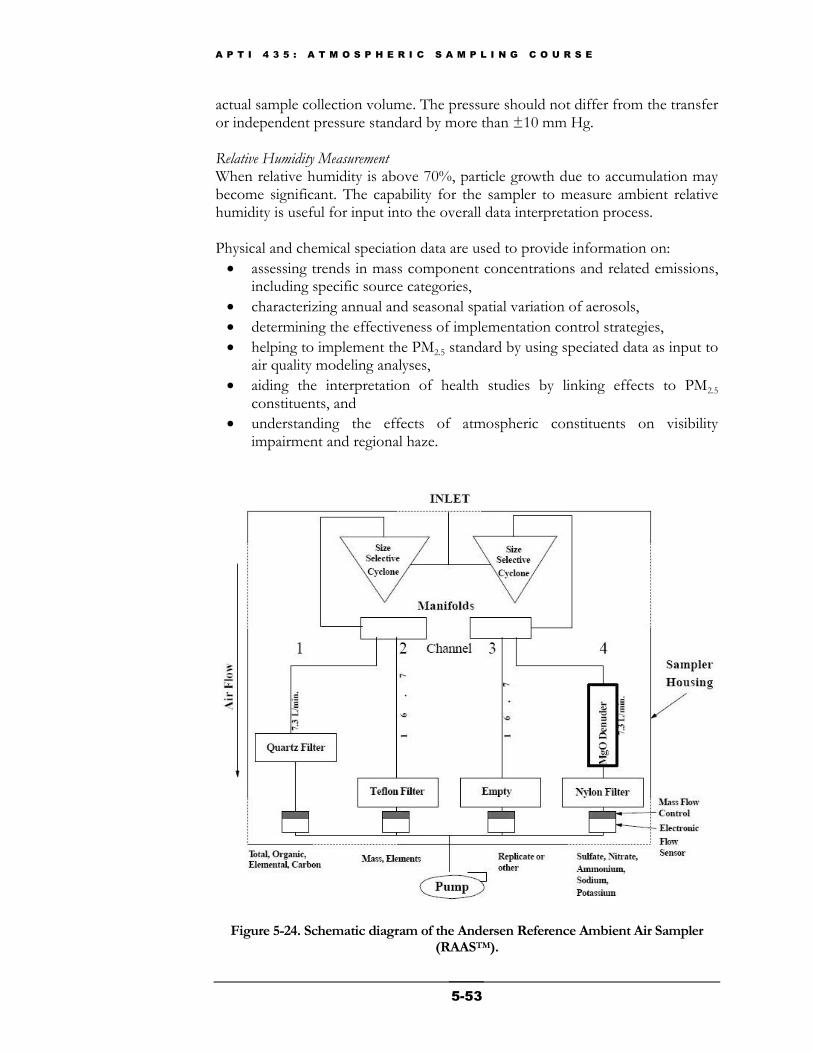
A P T I 4 3 5 : A T M O S P H E R I C S A M P L I N G C O U R S E
5-53
actual sample collection volume. The pressure should not differ from the transfer or independent pressure standard by more than ±10 mm Hg. Relative Humidity Measurement When relative humidity is above 70%, particle growth due to accumulation may become significant. The capability for the sampler to measure ambient relative humidity is useful for input into the overall data interpretation process. Physical and chemical speciation data are used to provide information on:
assessing trends in mass component concentrations and related emissions, including specific source categories,
characterizing annual and seasonal spatial variation of aerosols,
determining the effectiveness of implementation control strategies,
helping to implement the PM2.5 standard by using speciated data as input to air quality modeling analyses,
aiding the interpretation of health studies by linking effects to PM2.5 constituents, and
understanding the effects of atmospheric constituents on visibility impairment and regional haze.
Figure 5-24. Schematic diagram of the Andersen Reference Ambient Air Sampler (RAASTM).
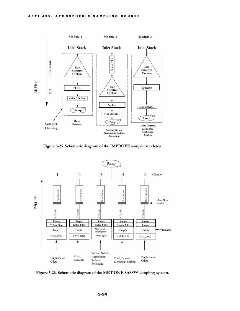
A P T I 4 3 5 : A T M O S P H E R I C S A M P L I N G C O U R S E
5-54
Figure 5-25. Schematic diagram of the IMPROVE sampler modules.
Figure 5-26. Schematic diagram of the MET ONE SASSTM sampling system.
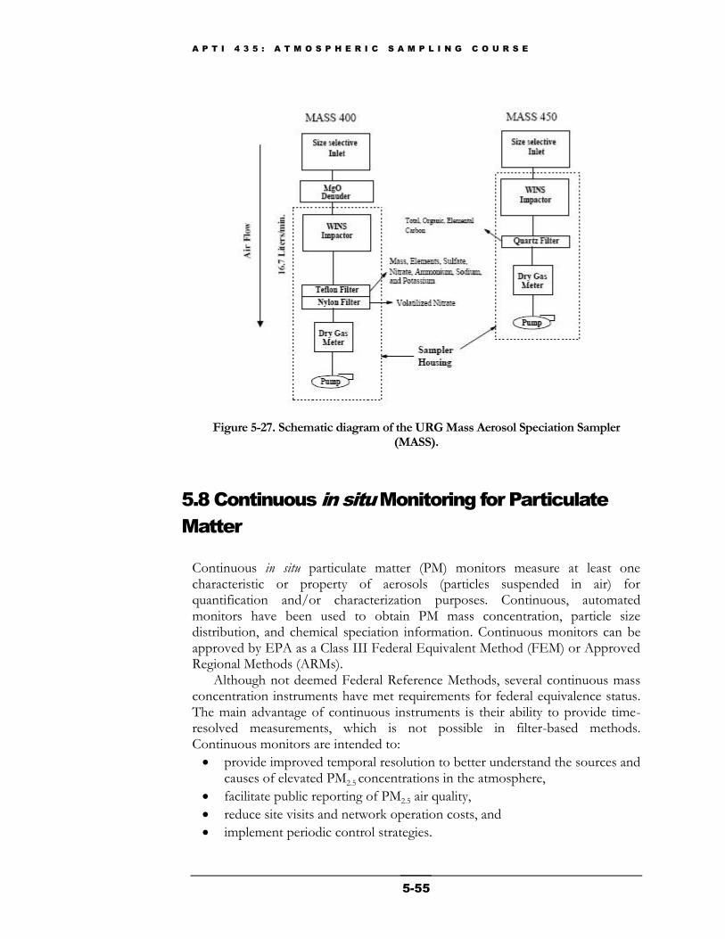
A P T I 4 3 5 : A T M O S P H E R I C S A M P L I N G C O U R S E
5-55
Figure 5-27. Schematic diagram of the URG Mass Aerosol Speciation Sampler (MASS).
5.8 Continuous in situ Monitoring for Particulate
Matter
Continuous in situ particulate matter (PM) monitors measure at least one characteristic or property of aerosols (particles suspended in air) for quantification and/or characterization purposes. Continuous, automated monitors have been used to obtain PM mass concentration, particle size distribution, and chemical speciation information. Continuous monitors can be approved by EPA as a Class III Federal Equivalent Method (FEM) or Approved Regional Methods (ARMs).
Although not deemed Federal Reference Methods, several continuous mass concentration instruments have met requirements for federal equivalence status. The main advantage of continuous instruments is their ability to provide time-resolved measurements, which is not possible in filter-based methods. Continuous monitors are intended to:
provide improved temporal resolution to better understand the sources and causes of elevated PM2.5 concentrations in the atmosphere,
facilitate public reporting of PM2.5 air quality,
reduce site visits and network operation costs, and
implement periodic control strategies.
A P T I 4 3 5 : A T M O S P H E R I C S A M P L I N G C O U R S E
5-56
Continuous PM measurements have a large role in NCore (National Core) and SLAMS (State and Local Air Monitoring Stations) air quality networks. Although the SLAMS network includes NCore, PAMS, and all other state or locally operated stations not designated as special purpose monitor (SPM) stations, not all SLAMS sites are NCore sites. For this reason, requirements for continuous monitoring instruments are discussed separately for NCore and SLAMS below.
National Core (NCore)
There is at least one NCore site in each state, and each NCore site, at a minimum, must be able to provide the following PM information: 1) PM2.5
particle mass using continuous and integrated/filter-based samplers, 2) speciated PM2.5, 3) PM10–2.5 particle mass, and 4) speciated PM10–2.5. Several sites are capable of continuous PM10-2.5 mass concentration. These sites are expected to complement the PM2.5 data collection that takes place at non-NCore/SLAMS sites, and both types of sites can be used to meet the minimum PM2.5 network requirements of NCore and/or SLAMS. Details on NCore can be found in 40 CFR Part 58 Appendix D and http://www.epa.gov/ttn/amtic/ncore/ index.html.
State and Local Air Monitoring Stations (SLAMS)
PM10-2.5 measurements are only required at SLAMS sites that additionally serve as NCore sites (PM10-2.5 is required at NCore sites). Consequently, SLAMS-only sites do not require continuous PM10 measurements, although continuous PM2.5 measurements are required. The minimum number of continuous PM2.5 monitors at SLAMS sites depends on the site’s Metropolitan Statistical Area classification (40 CFR Part 58 Appendix D, Table D-5). At least half of the PM2.5 samplers at each site must be a continuously monitoring instrument. Additionally, at least one required continuous analyzer in each Metropolitan Statistical Area must be collocated with an FRM/FEM/ARM monitor, unless the continuous instrument has already been deemed a FEM or ARM monitor. In such cases, no collocation with an additional FRM, FEM, or ARM sampler is required. A current list of USEPA reference and equivalent methods can be found at http://www.epa.gov/ttn/amtic/criteria.html.
5.9 Automated Federal Equivalent Monitors
Instruments using two different measurement principles have received EPA’s approval as equivalent methods (FEM) for PM10. The first uses beta-radiation; the second uses an oscillating pendulum. Although these instruments can provide high-quality, time-resolved PM2.5 data, automated equivalent methods have only recently been approved for PM2.5. These two measurement principles, now featured by several vendors, are briefly discussed below.
A P T I 4 3 5 : A T M O S P H E R I C S A M P L I N G C O U R S E
5-57
Beta Attenuation Monitor (BAM)
The beta attenuation monitor samples at ambient conditions of temperature, relative humidity, and gas concentration to minimize particle volatilization biases. These monitors operate at a manufacturer-specified flow rate using an inlet hat, impactor, or cyclone to determine the 50% cut-point for the desired particle size to be measured. For beta attenuation monitors, low-energy, electron-emitting beta rays from a radioactive source are focused on sample deposits on a filter tape and detected on the opposite side. The beta intensity is described, to a good approximation, by the Beer-Lambert relationship. Common radioactive beta sources are Carbon-14 (C-14) and Krypton-85 (Kr-85), although Carbon-14 is more commonly used.
A continuous filter, commonly composed of glass fiber, is used in beta attenuation monitors. Typically, the attenuation through an unexposed portion of the filter tape is measured, and the tape is then exposed to the ambient sample flow where a deposit is accumulated. The beta attenuation is repeated, and the difference in attenuation between the blank filter and the deposit is a measure of the accumulated concentration.
A continuous measurement of aerosol mass concentration becomes possible when the beta attenuation coefficient per aerosol mass deposited on the filter is known. For example, the attenuation coefficient is ~0.26 cm2/mg for typical atmospheric aerosol using a Carbon 14 source. In continuous monitoring, movement of the filter tape is needed when the aerosol loading on the deposition spot attenuates the beta intensity at the detector to near background levels. Blank-corrected attenuation readings can be converted to mass concentrations for averaging times as short as 30 minutes. While these monitors are capable of producing half-hourly average mass concentrations, a 24-hour averaging period is required for typical ambient concentrations to obtain sufficient particulate deposition for accurate determination.
BAMs are typically operated at ambient temperatures and relative humidity. While these conditions preserve the integrity of volatile nitrates and organic compounds, they also favor the sampling of liquid water associated with soluble species at high humidities. Under these conditions BAM concentrations are often larger than those of collocated filter samplers for which samples have been equilibrated at lower laboratory relative humidities prior to gravimetric analysis. Sampled air can be preceded by a diffusion dryer to remove water vapor, thereby encouraging the evaporation of liquid water associated with soluble components of suspended particles.
A schematic of the beta attenuation measurement principle is shown in Figure 5-28:
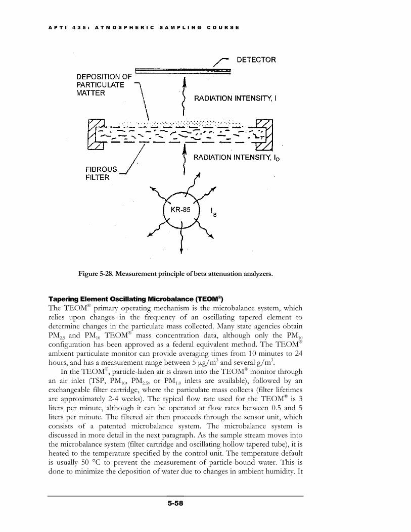
A P T I 4 3 5 : A T M O S P H E R I C S A M P L I N G C O U R S E
5-58
Figure 5-28. Measurement principle of beta attenuation analyzers.
Tapering Element Oscillating Microbalance (TEOM®
)
The TEOM® primary operating mechanism is the microbalance system, which relies upon changes in the frequency of an oscillating tapered element to determine changes in the particulate mass collected. Many state agencies obtain PM2.5 and PM10 TEOM® mass concentration data, although only the PM10 configuration has been approved as a federal equivalent method. The TEOM® ambient particulate monitor can provide averaging times from 10 minutes to 24 hours, and has a measurement range between 5 μg/m3 and several g/m3.
In the TEOM®, particle-laden air is drawn into the TEOM® monitor through an air inlet (TSP, PM10, PM2.5, or PM1.0 inlets are available), followed by an exchangeable filter cartridge, where the particulate mass collects (filter lifetimes are approximately 2-4 weeks). The typical flow rate used for the TEOM® is 3 liters per minute, although it can be operated at flow rates between 0.5 and 5 liters per minute. The filtered air then proceeds through the sensor unit, which consists of a patented microbalance system. The microbalance system is discussed in more detail in the next paragraph. As the sample stream moves into the microbalance system (filter cartridge and oscillating hollow tapered tube), it is heated to the temperature specified by the control unit. The temperature default is usually 50 °C to prevent the measurement of particle-bound water. This is done to minimize the deposition of water due to changes in ambient humidity. It
A P T I 4 3 5 : A T M O S P H E R I C S A M P L I N G C O U R S E
5-59
should be noted, however, that a default temperature of 50 °C can volatilize most of the ammonium nitrate and some of the volatile organic compounds in atmospheric particles. Consequently, monitored sites and seasons having high levels of ammonium nitrate and/or organic particulate mass do not always yield a reasonable correspondence between time-integrated TEOM® and collocated filter measurements.
The TEOM® microbalance system is quite unique. The TEOM® draws air through a hollow tapered tube, with the wide end of the tube fixed, while the narrow end oscillates in response to an applied electric field. The narrow end of the tube carries the filter cartridge. The sampled air stream passes from the sampling inlet, through the filter and tube, to a flow controller. The tube-filter unit acts as a simple harmonic oscillator described by the following equation:
(Eq. 5-6)
0.5
m
kω
Where: ω = the angular frequency, k = the restoring force constant, and m = the oscillating mass
As particles are collected on the filter, the oscillating mass changes and results in a change of the oscillating frequency. An electronic control system maintains the tapered tube in oscillation and continuously measures this oscillating frequency. Basically, changes in PM mass are correlated to changes of the TEOM® oscillating frequency. To calibrate the system, the restoring force constant (k) is determined by placing a gravimetrically determined calibration mass on the filter and recording the frequency change due to this mass.
Details regarding the operation, calibration, and maintenance of several EPA-approved continuous and filter-based instruments can be found at the following website: http://www.epa.gov/ttn/amtic/inorg.html.
5.10 Other Automated PM Methods
Several other automated methods have been developed and used by researchers and air pollution professionals in order to better characterize particulate matter. These methods, described below, have been used for a variety of purposes, including outdoor and indoor air monitoring, industrial hygiene, and personal exposure assessment. Although many of the following methods are not commonly used by federal, state, local, and tribal agencies, they can be quite useful in obtaining time-resolved or semi-continuous information on mass concentration, total number of particles in specific size ranges, and elemental composition of particulate matter. In fact, continuous instruments measuring mass concentration may receive future approval as Class III FEMs, and can possibly be used as ARMs by state, local, and tribal agencies.
A P T I 4 3 5 : A T M O S P H E R I C S A M P L I N G C O U R S E
5-60
All continuous monitoring methods not previously discussed are discussed below by measurement principle. Much of the information presented below is based on the following EPA document: Guidance for Using Continuous Monitors in PM2.5 Monitoring Networks (March 3, 1998). This document can be found at the following URL: http://www.epa.gov/ttnamti1/files/ambient/pm25/r-98-012.pdf. Detailed information regarding each instrument can be found via sources cited within the text of the Guidance document.
Mass and Mass Equivalent
In mass and mass equivalent instruments, particle mass is determined by its inertia, electron attenuation properties, or by the decrease in pressure across small pores in a filter. In addition to the Beta Attenuation Monitor (BAM) and Tapering Element Oscillating Microbalance® (TEOM®) discussed in the previous section, two commonly used mass and mass equivalent instruments are discussed below. Piezoelectric Microbalance Piezoelectric crystals have mechanical resonances that can be excited by applying an alternating electrical voltage to the crystal. As the resonance frequencies are very well defined, such crystals (quartz in particular) have found applications as secondary time and frequency standards in clocks and watches. As for all mechanical resonators, the resonance frequency is a function of mass. Therefore, by monitoring the resonance frequency in comparison with a second crystal, one can continuously measure the mass deposited on the crystal. Comparison with a second crystal largely compensates for the effect of temperature changes on the resonance frequency.
The piezoelectric principle has been used to measure particle mass by depositing the particles on the crystal surface either by electrostatic precipitation or by impaction. The collection efficiency of either mechanism has to be determined as a function of particle size to achieve quantitative measurements. In addition, the mechanical coupling of large particles to the crystal is uncertain. Both single and multi-stage impactors have been used to collect particles by size range. Quartz crystals have sensitivities of several hundred hertz per microgram. This sensitivity results in the ability to measure the mass concentration of a typical 100 µg/m3 aerosol to within a few percent in less than one minute. Pressure Drop Tape Sampler (CAMMS) A continuous particle mass monitoring system, CAMMS (continuous ambient mass monitor system), is based on measuring the pressure drop across a porous Fluoropore membrane filter. This pressure drop is linearly correlated to the particle mass deposited on the filter. The filter face velocity is chosen such that pore obstruction by interception is the dominant cause of particle-related pressure drop change over time. The monitor consists of: 1) a Fluoropore filter tape to collect particles; 2) a filter tape transportation system to allow for several weeks of unattended particle sampling; 3) a system to measure the pressure drop across the filter; 4) a diffusion dryer to remove particle-bound water; and 5) an air sampling pump. The monitor exposes a new segment of filter tape every 20 to
A P T I 4 3 5 : A T M O S P H E R I C S A M P L I N G C O U R S E
5-61
60 minutes for particle collection. During this period, particles collected on the filter should remain in equilibrium with the sample air, since the composition of ambient air does not usually vary substantially over this short time period. Volatilization and adsorption artifacts are minimized because measurements are made at ambient temperature for short time periods and at a low face velocity. A diffusion dryer that removes water vapor could also be used to condition air, thereby encouraging the evaporation of liquid water associated with soluble components of suspended particles. The CAMMS can detect concentrations as low as 2 μg/m3 for hourly averaged measurements.
Visible Light Scattering
Particle light scattering (bsp) is determined by illuminating particles, individually or as a group, and measuring the scattered intensity at different orientations from the incident light source. The intensity of scattered light is related to mass concentration by electromagnetic theory or by comparison with a collocated filter measurement. Particle light scattering measurements from five different types of instruments are discussed in the following subsections. Nephelometer Nephelometers, as a whole, are highly versatile instruments that quantify particle light scattering. Integrating nephelometers quantify particle light scattering integrated over all directions. For visibility applications, scattering extinction serves as a surrogate for total light extinction which is related to visibility.
Other applications of the integrating nephelometer include: 1) measurements of Rayleigh scattering coefficients, 2) determination of aerosol size distributions and refractive indices, 3) detection of sulfuric acid - ammonium sulfate aerosol; and 4) estimation of particle mass concentrations. Nephelometer sampling procedures depend on the intended uses of the data. To determine visibility reduction, total light scattering is desired, including light scattering caused by 1) liquid water associated with soluble particles and 2) molecules in clean air.
Mass concentration measurements from nephelometers are typically overestimated once relative humidity is above 80%. This is due to the fact that small particles grow to sizes that scatter light more efficiently as they acquire liquid water at approximately 80% relative humidity. To compensate for this, the air stream can be heated, similar to TEOM® air conditioning, to remove liquid water when an indicator of particle mass is desired. Some systems are able to control both temperature and humidity to characterize the hygroscopic properties of suspended particles. Such heating mechanisms, however, can increase the volatilization of ammonium nitrate and volatile organic compounds from particles. Although light scattering is often highly correlated with mass concentrations, this relationship depends on several variables and may be different from location to location and for different seasons of the year.
Particle scattering measured by integrating nephelometers includes systematic errors owing to: 1) non-monochromatic light sources; 2) limits of the integration angle; and 3) and non-Lambertian light sources. Further modification of the
A P T I 4 3 5 : A T M O S P H E R I C S A M P L I N G C O U R S E
5-62
nephelometer response can also be achieved by adding a size-selective inlet to the nephelometer air intake. Optical Particle Counter (OPC) Optical Particle Counters (OPC) use light scattering to detect the size and number of individual particles. OPCs have long been used in aerosol research, thereby attaining a degree of reliability and ease of operation that allow them to be deployed in long-term monitoring networks. Some instruments analyze the spatial distribution of the scattered light to derive a shape parameter that can be used to determine deviations from sphericity.
In an OPC, a narrow air stream is directed through a small sensing zone, where it is illuminated by an intensive light beam, commonly a visible laser beam. Light scattered by an individual particle is sensed by a fast and sensitive detector, resulting in an electrical pulse. Particle size is determined from the pulse amplitude, and particle number is determined from the number of pulses. The size of particles that can be detected with OPCs ranges from about 0.05 to 50 µ, but it is more typically 0.2 to 30 µm.
Particle sizes and numbers are translated to mass concentration by assuming a spherical particle shape and a particle density. The sum over all particle size bins can be further related to mass loadings by comparison with a collocated filter sample. Some particle counters allow a 47-mm filter to be placed in the exhaust stream so that the sensed particles can be collected for laboratory weighing and possible chemical characterization.
A purge filter is typically used to pre-zero the OPC before each set of measurements is taken. Once a year, the OPC is typically sent to the manufacturer for calibration with a National Institute of Standards and Technology (NIST)-traceable, monodisperse distribution of polystyrene latex spheres. While size measurements with OPCs can be very precise, their accuracy depends on particle composition and shape. These issues have been explored for atmospheric aerosols. Accuracy can be improved by simultaneous use of an integrating nephelometer with optical particle counters. Condensation Nuclei Counter (CNC) Continuous-flow Condensation Nuclei Counters (CNC) sense ultrafine particles by causing them to grow to a size that is efficiently detected by light scattering. Particles in a sampled air stream enter a saturator where alcohol vapors at a temperature typically above ambient (e.g., 35 °C) create a saturated atmosphere. Particles then pass into a condenser tube at a temperature sufficiently below that of the saturator (e.g., 10 °C). Alcohol vapor condenses on the particles causing them to grow, and they are detected and classified by an OPC. CNCs detect particles with 0.003 to 1 μm diameters. For low particle concentrations, the instrument operates in a counting mode, registering individual light pulses. For concentrations above 1,000 particles/cm3, the simultaneous presence of more than one particle in the viewing volume becomes frequent, and individual particles can no longer be counted. At this point, the CNC switches to the photometric mode where the power of the light scattered by all particles present in the viewing volume is measured. In the counting mode, a CNC can be very precise, but the counting efficiency for ultrafine particles depends substantially
A P T I 4 3 5 : A T M O S P H E R I C S A M P L I N G C O U R S E
5-63
on the instrument design. In the photometric mode, the CNC must be calibrated with an aerosol of known concentration (for example, by using an electrostatic classifier). Response curves as a function of particle size, concentration, and different environmental conditions have been determined for several different CNCs.
CNCs are the most practical instruments for determining ultrafine particle concentrations, but they are not as accurate as other continuous methods for determining PM2.5 or larger size fractions owing to the low upper limit of their size range. Aerodynamic Particle Sizer (APS) The Aerodynamic Particle Sizer (APS) measures light scattering as well as the time-of-flight of sampled particles. The measured aerodynamic diameter can be converted to volume-equivalent diameter or mobility-equivalent diameter. The APS accelerates the air stream in a converging nozzle. Particles have a larger inertia than the gaseous component, and therefore lag in acceleration and speed behind the air stream. Particles with higher mass (as a result of higher density or larger size) achieve lower velocities than those with lower mass. Each particle is detected by laser scattering at the beginning and end of a fixed path length to determine the time taken to traverse this path (the ―time-of-flight‖). The flight times are related to particle mass. The APS measures particles with diameters of 0.5 to 30 μm.
The APS aerodynamic diameter differs from the standard definition of aerodynamic diameter (the diameter of the unit density sphere that has the same settling velocity in still air). The APS aerodynamic diameter is adjusted for particle density, ambient gas density, and ambient air viscosity. During the acceleration process, calibration and ambient particles can deform in different ways (i.e., flatten) depending on their viscosity. Nonspherical particles behave differently from spherical particles, necessitating additional adjustments. Phantom particle counts may result from the time-of-flight laser detection system. Light Detection and Ranging (LIDAR) Light Detection and Ranging (LIDAR) measures light scattered in the direction of the light source (―backscattering‖) along a sight path. Aerosol LIDAR determines aerosol distributions while Differential Absorption LIDAR (DIAL) can measure concentrations of several gases.
Several types of LIDAR are currently in-use. Basic single-wavelength aerosol LIDAR yields a semi-quantitative measurement of the backscatter coefficient. High-spectral-resolution and Raman LIDAR provide quantitative backscatter coefficients; these systems are very complex and currently not commercially available. The connection between backscatter coefficient and PM concentration is indirect and depends on particle size distribution and refractive index of the aerosol particles, similar to nephelometers. Aerosol LIDAR are more suitable for determining the spatial distribution of aerosol concentrations and its temporal development, than for quantifying mass concentrations.
A basic aerosol LIDAR system consists of a transmitter and a receiver located next to each other. The transmitter, typically a pulsed laser, sends a short
A P T I 4 3 5 : A T M O S P H E R I C S A M P L I N G C O U R S E
5-64
pulse of collimated light into the atmosphere. A small part of this light pulse is scattered back into the receiver by suspended particles and gas molecules. The absolute system calibration is generally unknown. The LIDAR equation is, therefore, under-determined and cannot be solved without additional assumptions or data.
DIAL measurements are made at two different wavelengths with substantially different absorption coefficients for the gas of interest. DIAL LIDAR is a useful tool for continuous measurements of aerosol precursor gases. The range-resolved gas concentration is calculated from the ratio of the LIDAR signals at the two wavelengths. The laser line wavelength with the larger absorption coefficient is referred to as ―on-line.‖ The laser line with the smaller absorption coefficient is referred to as ―off-line.‖
DIAL has been used for the measurement of a number of relevant tropospheric trace gases including ozone (O3), sulfur dioxide (SO2), nitric oxide (NO), nitrogen dioxide (NO2), ammonia, and aromatic hydrocarbons. Though commercially available, LIDAR systems are expensive and must be individually designed or modified for each specific application.
Visible Light Absorption
Black carbon (BC) (sometimes termed ―elemental carbon,‖ ―light-absorbing carbon,‖ or ―soot‖) is the dominant visible light-absorbing particulate species in the troposphere and mostly results from anthropogenic combustion sources. It is usually found in the nucleation or accumulation mode for particles well under 1 μm in equivalent dimensions (i.e., if chain aggregates were consolidated into a single sphere). Mass loadings range from a few ng/m3 in remote pristine regions or over oceans distant from land, to a fraction of 1 μg/m3 in rural regions of the continents, and exceed 1 μg/m3 in many cities.
Continuous methods that monitor particle light absorption (bap) can also be used to measure the PM2.5 component consisting of light-absorbing particles. Attenuation of light through a filter and photoacoustic oscillation are detection principles used to quantify particle absorption as a surrogate for black carbon. Particle light absorption measurements from three different instruments are discussed in the following subsections. Aethalometer and Particle Soot/Absorption Photometers Light-absorbing aerosol (e.g., BC) deposited on a filter can be quantified through the measurement of light transmission or reflection. For example, initial methods, such as the British Smoke method in the early 1950s, were first used to visually characterize the reflectance of a filter sample. In their more advanced configurations, a clean portion of a filter tape was periodically moved into the sampling position, thereby allowing diurnal variations (typically hourly averages) in particle concentrations to be recorded. In these methods, the optical density of the particle deposit is determined from the logarithm of the ratio of intensities measured on the filter with and without the deposit.
A more quantitative method, the integrating sphere method, measures aerosol light absorption by placing the loaded filter in an integrating sphere and illuminating it. Light, both transmitted and scattered by the loaded filter, first
A P T I 4 3 5 : A T M O S P H E R I C S A M P L I N G C O U R S E
5-65
reaches the diffusely reflecting surface of the sphere where it is homogenized, and then the light is detected by the photodetector. The difference between a clean filter and one loaded with particles gives the amount of light absorbed by the particles. Simplifications of the integrating sphere method, such as the integrating plate or sandwich methods, are most often used for routine measurements.
A real-time version of the integrating plate method, the aethalometer, continuously collects aerosol on a quartz-fiber filter tape. During the deposition process, the light attenuation through the aerosol collection spot and an unloaded reference spot are monitored. Their difference yields the absorption due to the integral of all light-absorbing materials collected on a particular spot. The time derivative of this quantity is a measure of the current aerosol light absorption. When the optical density of the aerosol spot reaches a certain value, the filter tape advances automatically. Time resolution available with the aethalometer varies from seconds or minutes in urban areas to ten minutes in rural locations and longer in very remote locations. One filter tape is sufficient for approximately 700 aerosol collection spots corresponding to one or more months of operation in urban areas, or a year or more in rural areas.
The aethalometer converts the result of its filter attenuation measurement into BC mass concentration by a conversion factor of 19.2 m2/g. Aethalometer BC generally agrees well with collocated filter samples analyzed for elemental carbon by thermal optical methods. Applications of the aethalometer include air quality monitoring in urban and more remote locations, transport studies, and source characterization.
The Particle Soot/Absorption Photometer (PSAP) gives a filter-based, real-time measurement of aerosol light absorption. The PSAP produces a continuous measurement of absorption by monitoring the change in transmittance across a filter for two areas on the filter, a particle deposition area and a reference area. A light emitting diode (LED) operating at 550 nm, followed by an Opal glass, serves as light source. The absorption reported by the PSAP is calculated with a nonlinear equation correcting for the magnification of absorption by the filter medium and for response nonlinearities as the filter is loaded. Measurement time resolution can be as short as a few seconds to five minutes, depending on ambient aerosol light absorption. Applications of the PSAP include its use in ground-based monitoring by NOAA’s Climate Monitoring and Diagnostics Laboratory (CMDL) and in field campaigns such as the Aerosol Characterization Experiment (ACE) of the International Global Atmospheric Chemistry (IGAC) program. Photoacoustic Spectroscopy At atmospheric pressures, electromagnetic energy absorbed by particles changes to thermal energy, thereby heating the particles and the surrounding gases. Increased gas temperatures surrounding light-absorbing particles cause thermal expansion of the gas. When the light source power is modulated, the periodic expansion of the gas results in a sound wave at the modulation frequency, which may be detected with a microphone. This ―photoacoustic‖ detection of particle light absorption can be related to the black carbon concentration.
A P T I 4 3 5 : A T M O S P H E R I C S A M P L I N G C O U R S E
5-66
Sensitive photoacoustic techniques use a power-modulated laser as light source. By placing the aerosol-laden air into an acoustic resonator, and modulating the laser power at its resonance frequency, the varying pressure disturbance (acoustic signal) is amplified by the buildup of a standing acoustic wave in the resonator.
Electrical Mobility
Electrical mobility analyzers are applicable to particles smaller than 1 μm. They are the only practical alternative to the Condensation Nuclei Counter (CNC) instrument for quantifying the ultrafine fraction of the particle size distribution. The resulting particle size is known as mobility equivalent diameter, which can be converted to volume equivalent diameter or aerodynamic diameter.
A basic electrical mobility analyzer consists of: 1) a charger to impart an electric charge to the particles (a diffusion charger that exposes particles to unipolar positive ions is commonly used); 2) a classifier that separates the particles by acting on their electrical charge and mass; and 3) a detector to monitor the separated particles.
Electrical mobility analyzers are often used together with aerodynamic particle sizers, with the electrical mobility analyzer capturing particles below 1 μm and the aerodynamic particle sizers measuring the larger particles. Particle number measurements with two different instruments are discussed in the following subsections. Electrical Aerosol Analyzer (EAA) The Electrical Aerosol Analyzer (EAA) has been widely applied and characterized in aerosol studies. EAAs are typically operated with about ten size channels covering the range from 0.01 to 1.0 μm with a measurement time on the order of a few minutes.
A positively charged aerosol enters a mobility tube consisting of two coaxial cylinders. The outer tube is grounded and a negative potential is applied to the inner tube. As the aerosol flows down the mobility tube, its mobile fraction is precipitated on the inner tube by electrical forces. The remaining aerosol is detected, commonly by an electrometer that measures the electrical current of the remaining aerosol. The potential (voltage) of the inner cylinder is changed in steps. For each potential, a different fraction of the aerosol is precipitated. The resulting current-versus-voltage curve for an aerosol can be converted into a current-versus-size curve once the EAA has been calibrated with monodisperse aerosol of known size. Calibration of the current sensitivity is done by grounding the inner cylinder and measuring the aerosol current without precipitation losses. Differential Mobility Particle Sizer (DMPS) The Differential Mobility Particle Sizer (DMPS) improves on the EAA by making measurements with much greater size resolution (e.g., 100 channels).
The DMPS is essentially a modification of the EAA. The basic difference is that the DMPS produces a flow of aerosol consisting of particles with an electrical mobility between two closely spaced values (i.e., differential), while the EAA produces a flow consisting of particles with an electrical mobility above
A P T I 4 3 5 : A T M O S P H E R I C S A M P L I N G C O U R S E
5-67
some value (i.e., integral). Instead of measuring the flow of particles missing the inner tube as in the EAA, a sample flow of aerosol is extracted through a slot in the inner tube. Only particles with mobilities within a limited range enter the sample stream for detection. As in the EAA, the voltage of the inner tube is stepped through a number of values and the DMPS directly yields the electrical mobility distribution without further differentiation.
Measurement times for DMPS with electrometers as detectors can be on the order of one hour. Operation with a CNC as a detector can reduce the measurement time by an order of magnitude. A further order of magnitude reduction in averaging time can be achieved by scanning the inner tube voltage. This modification is referred to as a Scanning Mobility Particle Analyzer (SMPA).
The conventional DMPS utilizing a cylindrical geometry is limited for ultrafine particles (< 0.020 μm) as its transmission efficiency drops dramatically below 0.02 μm due to diffusion losses. The accessible size range can be extended down to 0.001 μm by either modifying the cylindrical DMPS or by changing to a radial geometry.
Chemical Components
If the carbonaceous, nitrate, sulfate, ammonium, and geological components of suspended particles could be determined continuously and in situ, a reliable speciated estimate of PM2.5 or PM10 mass concentration could be derived. While most of these chemical-specific particle monitors are currently experimental, rapid technology advances will make them more available and more widely used within coming years. The following subsections introduce various versions of single particle mass spectrometers that measure particle size and chemical composition, along with single compound instruments to measure carbon, sulfur, and nitrate. Single Particle Mass Spectrometers Continuous versions of the Laser Microprobe Mass Spectrometer (LAMMS) have been developed as the Rapid Single particle Mass Spectrometer (RSMS), Particle Analysis by Laser Mass Spectrometry (PALMS), and Aerosol Time Of Flight Mass Spectrometry (ATOFMS). These devices measure the size and chemical composition of individual particles. More recently, instruments have been developed for ground-based monitoring and monitoring in the troposphere and lower stratosphere.
In SPMS analyzers, particles are introduced into a vacuum by a nozzle. The presence of particles is detected through light scattered from a visible laser beam. This scattering process is also used as an Optical Particle Counter (OPC) or Aerodynamic Particle Sizer (APS) to determine the size and number of particles passing through the instrument. The presence of a particle triggers a high-energy pulsed laser which, with a single pulse, vaporizes particle material and ionizes part of it. The ions are detected and analyzed by a time-of-flight mass spectrometer. The time particles spend in the vacuum is on the order of microseconds, minimizing condensation, evaporation, and reactions.
The analysis rate is limited by the repetition rate of the pulsed laser. The presence of the OPC makes it possible to analyze a size-selected fraction of the
A P T I 4 3 5 : A T M O S P H E R I C S A M P L I N G C O U R S E
5-68
particles; however, it also imposes a lower limit on the particle size being analyzed, as very small particles are not detected by the OPC. Running a pulsed laser without triggering can acquire smaller particles, but at the expense of a lower duty cycle and no size selection. Because of the complicated ionization process, the technique is currently used more commonly to survey the chemical composition of particles than to yield quantitative mass concentrations of particle components.
Applications of this technique have included characterizing aerosol composition, examining the purity of laboratory-generated sulfuric acid droplets, determining halogens, speciating sulfur, studying matrix-assisted laser desorption/ionization, monitoring pyrotechnically-derived aerosol in the troposphere, characterizing automotive emissions, measuring marine aerosols and their radiative properties, and observing heterogeneous chemistry. Carbon Analyzer Various analyzers have been developed to determine ambient organic carbon (OC) and elemental carbon (EC). As previously mentioned, elemental carbon (EC), also known as black carbon (BC), can be measured by aethalometers. A recently available device, the multi-angle absorption photometer, has been designed to carry out continuous emission measurements of EC. This instrument measures atmospheric loading using a radiative transfer scheme to particle-loaded glass fiber filters. The EC content of collected particles on the filter tape is continuously determined at several angles by simultaneously measuring optical absorption and scattering of light. Detection limits for the multi-angle absorption photometer are as low as 100 ng/m3 for a 2-minute sample and 20 ng/m3 for a 30-minute sample. Various inlets (TSP, PM10, PM2.5, PM1.0) are available for the multi-angle absorption photometer and other carbon analyzers.
A thermal method has been used in the past to determine hourly-averaged, continuous particulate OC and EC concentrations. Specifically, the Ambient Carbon Monitor Series 5400 by Rupprecht and Patashnick, Co., now discontinued, differentiated between OC and EC by dividing the measured amount of carbon released from an intermediate burn (default 250 °C) and a final burn (default 750°C), respectively, by the air volume that passed through the instrument during sample collection. Volatilized carbon in this instrument was detected by a NDIR CO2 sensor. These instruments provide hourly, continuous measurements by collecting particles on one impaction collector (collection mode) while the other impaction collector is in analysis mode.
Thermal/optical methods have been typically used for semi-continuous measurements of both OC and EC. These instruments are considered semi-continuous since sample collection and the internal analysis of the collected sample cannot simultaneously occur. Typically, all carbon in the sample is converted to methane (CH4) for quantification by a Flame Ionization Detector (FID). For a 30-minute sample, the minimum quantifiable levels are 0.5 µg/m3 for OC and EC, respectively. Sulfur Analyzer Continuous methods for the quantification of particulate sulfur compounds first remove gaseous sulfur (e.g., SO2, H2S) from the sample stream by a diffusion
A P T I 4 3 5 : A T M O S P H E R I C S A M P L I N G C O U R S E
5-69
tube denuder, followed by the analysis of particulate sulfur. Another approach is to measure total sulfur and gaseous sulfur separately by alternately removing particles from the sample stream, and aerosol sulfur is obtained as the difference between the total and gaseous sulfur. The total sulfur content is measured by a flame photometric detector (FPD) by introducing the sampling stream into a fuel-rich hydrogen-air flame that reduces sulfur compounds and measures the intensity of the S2* chemiluminescence.
Because the formation of S2* requires two sulfur atoms, the intensity of the chemiluminescence is theoretically proportional to the square of the concentration of molecules that contain a single sulfur atom. In practice, the relationship is between linear and square and depends on the sulfur compound being analyzed. Calibrations are performed using both particles and gases as standards. The FPD can also be replaced by a chemiluminescent reaction with ozone that minimizes the potential for interference with a faster time response.
Capabilities added to the basic system include in situ thermal analysis and sulfuric acid (H2SO4) speciation. Sensitivities for sulfur aerosols as low as 0.1 μg/m3 with time resolution ranging from 1 to 30 minutes have been reported. Continuous measurements of aerosol sulfur content have also been obtained by on-line x-ray fluorescence analysis with a time resolution of 30 minutes or less. Nitrate Analyzer The Automated Particle Nitrate Monitor (APNM) provides a high-time-resolution measurement of particle nitrate concentration. It uses an integrated collection and vaporization cell whereby particles are collected by a humidified impaction process, and analyzed in place by flash vaporization in a nitrogen carrier gas. In the vaporization process, the evolved gases from particulate origin are quantified by a chemiluminescent analyzer operated in the NOx mode. Time resolution of the instrument is on the order of 12 minutes, corresponding to a ten-minute collection followed by an analysis step of less than two minutes.
The humidifier plus flash vaporization approach is, in fact, similar to some manual methods for measuring the size distribution of sulfate aerosols. The difference, however, is that the particle collection and analysis has been combined into a single cell, thus allowing the system to be automated. Although the APNM method is specific to nitrate, the same technology could be applied for continuous sulfate measurements by using a sulfur detector instead of a nitric oxide detector.
Multi-Elemental Analyzer
Both streaker (PIXE International, Tallahassee, FL) and DRUM (Davis Rotating-drum Universal-size-cut Monitoring impactor) (University of California, Davis, CA) samplers provide continuous particle collection on filter substrates followed by laboratory elemental analysis with Particle-Induced X-Ray Emission (PIXE). This is a continuous but not an in situ real-time monitoring method, due to the lag time between sample collection and chemical analysis in a laboratory. These samplers have a time resolution of approximately one hour, and can supply high-time-resolution elemental concentrations.
A P T I 4 3 5 : A T M O S P H E R I C S A M P L I N G C O U R S E
5-70
Streaker Ambient particles in the streaker sampler are collected on two impaction stages and an after-filter. The first impaction stage has a 10-μm cutpoint and collects particles on an oiled frit that does not move. The particles collected on this stage are discarded. The second impaction stage has a 2.5-μm cutpoint and collects coarse particles (PM10 minus PM2.5) on a rotating Kapton substrate that is coated with Vaseline to minimize particle bounce. The second impaction stage is followed by a 0.4-μm-pore-size Nuclepore polycarbonate-membrane filter that has an 8-mm-long negative pressure orifice behind it to collect fine particles (nominally PM2.5). The air flow rate through the streaker sampler is primarily controlled by the porosity of the filter and the area of the negative pressure orifice. A 1-mm-wide orifice can be set up to result in a flow rate of approximately 1 liter per minute and produce an annular deposit of 8 mm in width, with any point on the deposit collected during a one-hour time period.
The body of the streaker sampler has a cylindrical form with a diameter of approximately 10 cm and a length of about 20 cm. It contains a clock motor that advances two particle collection substrates mounted within the streaker. The streaker is mounted in the open air with the sample air inlet at the bottom to keep out very large particles (e.g., rain and drizzle). Sample air flow rates can be verified by a flow meter, temporarily attached to the inlet of the streaker sampler at the beginning and end of sampling on each substrate, or at times in between. Substrates of 168 mm in length have the capacity to accommodate a seven-day sampling period. DRUM The Davis Rotating-drum Universal-size-cut Monitoring Impactor (DRUM) is an eight-stage cascade impactor. It collects particles on grease-coated mylar substrates that cover the outside circular surface of eight clock-driven slowly rotating cylinders or drums (one for each stage). The advantages of the DRUM sampler are its capability to operate for up to thirty days unattended and its use of the location of particle deposits along the drum substrate as a means to determine the time of their collection. The DRUM collects aerosol from 0.07 μm to 15 μm in diameter for eight size ranges (0.07 to 0.24, 0.24 to 0.34, 0.34 to 0.56, 0.56 to 1.15, 1.15 to 2.5, 2.5 to 5.5, 5.5 to 10, and 10 to 15 μm), followed by focused-beam PIXE analysis. DRUM samplers have been used in several visibility field studies to confirm assumptions about mass scattering efficiency dependence on sulfur size distributions (e.g., Pitchford and Green, 1997).
The DRUM sampler, and other Lundgren-type rotating drum impactors, are unique among size-segregating samplers in that they generate a continuous time history of aerosol component size distributions with short time resolution (e.g., hourly). Unlike the conventional aerosol size distribution data sets with at most a few dozen distributions that can be individually scrutinized, the DRUM produces hundreds of distributions. In addition, time series analysis, summary statistics, and multivariate analysis can be applied to concentrations measured on any or all stages of the DRUM sampler.
A P T I 4 3 5 : A T M O S P H E R I C S A M P L I N G C O U R S E
5-71
References
American Conference of Governmental Industrial Hygienists. 1985. Air sampling instruments. 8th edition. Cincinnati (OH): American Conference of Governmental Industrial Hygienists.
Appendix B to 40 CFR Part 50. 2008. Reference method for the determination of suspended particulate matter in the atmosphere (high-volume method), final rule. 40 CFR Part 50, Federal Register, Friday, April 17, 2008.
Appendix G to 40 CFR Part 50. 2008. Reference method for the determination of lead in suspended particulate matter collected from ambient air, final rule. 40 CFR Part 50, Federal Register, Friday, April 17, 2008.
Appendix J to 40 CFR Part 50. 2008. Reference method for the determination of particulate matter as PM10 in the atmosphere, final rule. 40 CFR Part 50, Federal Register, Friday, April 17, 2008.
Appendix L to 40 CFR Part 50. 2008. FRM for the determination of fine particulate matter as PM2.5 in the atmosphere, final rule. 40 CFR Part 50, Federal Register, Friday, April 17, 2008.
Appendix M to 40 CFR Part 50. 2008. FRM for the determination of particulate matter as PM10 in the atmosphere, final rule. 40 CFR Part 50, Federal Register, Friday, April 17, 2008.
Appendix O to 40 CFR Part 50. 2008. Reference method for the determination of coarse particulate matter as PM in the atmosphere, final rule. 40 CFR Part 50, Federal Register, Friday, April 17, 2008.
Appendix A to 40 CFR Part 58. 2008. Quality assurance requirements for SLAMS, SPMs and PSD air monitoring, final rule. 40 CFR Part 58, Federal Register, Friday, April 17, 2008.
Appendix C to 40 CFR Part 58. 2008. Ambient air quality monitoring methodology, final rule. 40 CFR Part 58, Federal Register, Friday, April 17, 2008.
Appendix D to 40 CFR Part 58. 2008. Network design criteria for ambient air quality monitoring, final rule. 40 CFR Part 58, Federal Register, Friday, April 17, 2008.
Bruckman L, Rubino. 1976. High-volume sampling: errors incurred during passive sample exposure periods. J Air Pollut Control Assoc 26:881.
Burton RM, Howard JN, Penley RL, Ramsay PA, Clark TA. 1972. Field evaluation of the high-volume particle fractionating cascade impactor - a technique for respirable sampling. Paper #72-30, presented at the 65th Annual Meeting of the Air Pollution Control Association, 18-22 June 1972.
A P T I 4 3 5 : A T M O S P H E R I C S A M P L I N G C O U R S E
5-72
Chahal HS, Romano DJ. 1976. High-volume sampling: effect of wind-borne particulate matter deposited during idle periods. J Air Pollut Control Assoc 26:885.
Chambers L. 1954. Filter media for air sampling. Industrial Hygiene Quarterly 15:290.
Chow JC. 1995. Critical review: measurement methods to determine compliance with ambient air quality standards for suspended particulate. JAWMA.
Chow JC, Watson JG. November 6, 1997. Guideline on speciated particulate monitoring. Special report prepared for U.S. Environmental Protection Agency, Research Triangle Park, NC 27711.
Cohen AL. 1973. Dependence of hi-vol measurements on airflow race. Environ Sci Tech 7:60-61.
Compendium of methods for the determination of inorganic compounds in ambient air. 1999. EPA/625/R-96/01a, July 1999. Available from: http://www.epa.gov/ttn/ amtic/inorg.html
Compendium of methods for the determination of toxic organic compounds in ambient air. 1999. EPA/625/R-96/010b, January 1999. Available from: http://www.epa.gov/ttn/amtic/files/ambient/airtox/tocomp99.pdf
Dams R, Heindrychx K. 1973. A high-volume sampling system for use with cellulose fibers. Atmos Environ 7:319.
Darns R, Rahn KA, Winchester JW. 1972. Evaluation of filter materials and impaction surfaces for nondestructive neutron activation analysis of aerosols. Environ Sci Tech 6:441.
Dzubay TG, Stevens RK. 1978. Dichotomous sampler - a practical approach to aerosol fractionation and collection. EPA 600/2-78-112.
Eastern Research Group, Inc. 2007 Feb. Technical assistance document for the National Ambient Air Toxics Trends and Assessment Program. Prepared for Michael N. Jones, U.S. Environmental Protection Agency, Office of Air Quality Planning and Standards (C304-06).
Kretzschmar JG. 1975. Comparison between three different methods for the estimation of the total suspended matter in urban air. Atmos Environ 9:931.
Lattore P, Silverman L. 1955. Collection efficiencies of filter papers for sampling lead fume. AMA Arch of Indust Health 11:243.
Lee KW, Ramamurthi M. 1993. Filter collection. In: Aerosol measurement: principles, techniques and applications. K. Willeke, P.A. Baron, editors. New York: Van Nostrand, Reinhold, pp. 179-205.
Lee RE, Goranson S. 1972. National air surveillance cascade impactor network, I. Size distribution measurements of suspended particulate matter in air. Environ Sci Tech 6:1019.
A P T I 4 3 5 : A T M O S P H E R I C S A M P L I N G C O U R S E
5-73
- - - 1972. Filter media and filter holders for air sampling. Air sampling instruments for evaluation of atmospheric contaminants. Cincinnati (OH): American Conference of Governmental Industrial Hygienists.
- - - 1995. Filters and filter holders. In: Air sampling instruments for evaluation of atmospheric contaminants. 8th ed. B. Cohen, S.V. Hering, editors. Cincinnati (OH): American Conference of Governmental Industrial Hygienists.
Lockhart LB Jr., Patterson RL Jr., Anderson WL. 1964. Characteristics of air filter media used for monitoring radioactivity. NRL Report 6054. Washington DC: U.S. Naval Research Laboratory.
Loo BW, Jaklevic JM, Goulding FS. 1976. Dichotomous virtual impactors for large scale monitoring of airborne particulate matter. In: Fine particles, B. Y. H. Liu, editor. pp. 311-350. New York: Academic Press.
Lundgren DA. 1967. An aerosol sampler for determination of particle concentration as a function of size and time. J Air Poll Control Assoc 17:225.
Magill PL, Holden FR, Ackely C, eds. 1956. Air pollution handbook. McGraw-Hill.
McKee HC, et al. 1972. Collaborative testing of methods to measure air pollutants, I. The high-volume method for suspended particulate matter. J Air Pollut Control Assoc 22:342.
MetOne Instruments, Inc. Beta attenuation monitor (BAM1020). February 24, 2000.
Mueller PK, Twiss S, Sanders G. 1972. Selection of filter media: an annotated outline. Presented at the 13th Conference on Methods in Air Pollution and Industrial Hygiene Studies, 30-31 October 1972.
Neustadter HE, et al. 1975. The use of Whatman-41 filters for high-volume air sampling. Atmos Environ 9:101.
Olin JG, Kurz JL. 1975. High-volume air sampling. Pollut Eng January 1975:30.
Paciga JJ, Jervis RE. 1976. Multielement size characterization of urban aerosols. Environ Sci Tech 10:1124.
Pate JB, Tabor EC. 1962. Analytical aspects of the use of glass fiber filters for the collection and analysis of atmospheric particulate matter. Am Ind Hyg Assoc J 23:144-145.
Peterson CM. 1972. Aerosol sampling and the importance of particle size. Air sampling instruments for evaluation of atmospheric contaminants. American Conference of Governmental Industrial Hygienists.
Picknett RG. 1972. A new method of determining aerosol size distributions from sampler data. Journal of Aerosol Science 3:189.
Ramskill E, Anderson W. 1951. The inertial mechanism in the mechanical filtration of aerosols. Journal of Colloid Science 6:416.
A P T I 4 3 5 : A T M O S P H E R I C S A M P L I N G C O U R S E
5-74
Robson CD, Foster KE. 1962. Evaluation of air particulate sampling equipment. Am Ind Hyg Assoc J 24:404.
Rupprecht and Patashnick Co., Inc. Series 5400 Ambient Carbon Particulate Monitor.
Setter LR, Zimmer CE, Licking DS, Tabor EC. 1961. Airborne particulate beta radioactivity measurements of the national air sampling network, 1953-1959. Am Ind Hyg Assoc J 22:19200.
Silverman L, Viles FG. 1948. A high-volume air sampling and filter weighing method for certain aerosols. J Indust Hyg and Toxicol 30:124.
Smith F, Nelson AC. June 1973. Guidelines for development of a quality assurance program-FRM for the determination of suspended particulates in the atmosphere (high-volume method). Prepared for Research Triangle Institute under Contract 68-02-0598.
Smith J, Surprenant N. Properties of various filtering media for atmospheric dust sampling. Proceedings of the American Society of Testing Materials 53:1122.
Stevens RK, Dzubay JG. 1978. Dichotomous sampler - a practical approach to aerosol fractionation and collection. EPA 600/2-78-112.
Tabor EC, Hauser TR, Lodge JP, Burtschell RH. 1958. Characteristics of the organic particulate matter in the atmosphere of certain American cities. AMA Arch Indust Health 17:58.
Thermo Electron Corporation. Multi Angle Absorption Photometer Model 5012, 2002.
U.S. Environmental Protection Agency, National Exposure Research Laboratory. List of designated reference and equivalent methods. April 17, 2008.
U.S. Environmental Protection Agency, Office of Air Quality Planning and Standards. 1998 May. Guidance for using continuous monitors in PM2.5
monitoring networks.
U.S. Environmental Protection Agency, Office of Air Quality Planning and Standards. 1999 Oct. Particulate matter (PM2.5) speciation guidance. Final draft, edition 1.
U.S. Environmental Protection Agency, Office of Air Quality Planning and Standards. 2007. Revisions to the ambient monitoring regulations: relevancy for the AIRNOW community. PowerPoint Presentation, National Air Quality Conferences.
U.S. Environmental Protection Agency, Office of Air Quality Planning and Standards. 2006 Oct. September 2006 final amendments to the national air quality monitoring requirements.
U.S. Environmental Protection Agency, Office of Research and Development. 1999 June. Compendium method IO-1: continuous measurement of PM10
A P T I 4 3 5 : A T M O S P H E R I C S A M P L I N G C O U R S E
5-75
suspended particulate matter (SPM) in ambient air. Compendium of methods for the determination of inorganic compounds in ambient air.
U.S. Environmental Protection Agency, Office of Research and Development. 1999 June. Compendium method IO-1.1: determination of PM10 in ambient air using the Andersen continuous beta attenuation monitor. In: Compendium of methods for the determination of inorganic compounds in ambient air.
U.S. Environmental Protection Agency, Office of Research and Development. 1999 June. Compendium method IO-1.2: determination of PM10 in ambient air using the Thermo Environmental Instruments (formerly Wedding and Associates) continuous beta attenuation monitor. Compendium of methods for the determination of inorganic compounds in ambient air.
U.S. Environmental Protection Agency, Office of Research and Development. 1999 June. Compendium method IO-1.3: determination of PM10 in ambient air using a continuous Rupprecht and Patashnick (R&P) TEOM® particle monitor. Compendium of methods for the determination of inorganic compounds in ambient air.
U.S. Public Health Service. Air pollution on measurements of the national air sampling network—analysis of suspended particulates, 1957-1961. Public Health Service Publication No. 978. Washington DC.
Watson JG, et al. March 6, 1998 draft. Guidance for using continuous monitors in PM2.5 monitoring networks. Prepared for U.S. Environmental Protection Agency, Research Triangle Park, NC 27711.
Weinstock L. Monitoring rule implementation and updates. U.S. Environmental Protection Agency, Office of Air Quality Planning and Standards. MARAMA Monitoring Committee Meeting.