242

INAFOR 11D-029

INTERNATIONAL CONFERENCE OF INDONESIAN FORESTRY RESEARCHERS (INAFOR)

Section D Forest Assessment and Modelling

Method for Detecting of Forest Degradation Method Using Landsat Satellite Images To Support MRV REDD in Halimun Salak National Park

Sigit Nugroho

Paper prepared for The First International Conference of Indonesian Forestry Researchers (INAFOR)

Bogor, 5 – 7 December 2011

INAFOR SECRETARIAT Sub Division of Dissemination, Publication and Library

FORESTRY RESEARCH AND DEVELOPMENT AGENCY Jl. Gunung Batu 5, Bogor 16610

243

Method for Detecting of Forest Degradation Method Using Landsat Satellite Images To Support MRV REDD in Halimun Salak National Park

Sigit Nugroho

ABSTRACT

Detection of degraded forest using remote sensing data has more technical challenges. For Monitoring Reporting and Verification (MRV) on REDD mechanism in regional scale, detection method of forest degradation is required. The objective of this research is to develop an approptiate method to detect forest degradation in forest conservation area of Halimun Salak National Park (HSNP). Forest Canopy Density (FCD), maximum likelihood, fuzzy and belief dempster shafer classification method were used to classify forest density and to detect forest degradation. Accuracy evaluation of classification and detection were based on overall accuracy which obtained from ground sample plot. Canopy density, LAI, crown indicator, stand density and basal area (lbds) were used as field indicators. Accuracy classification among stand density with four classification methods was FCD 61%, maximum likelihood 57%, fuzzy 51% and belief dempster shafer 49%. Based on evaluation of overall accuracy classification among canopy density and four classification method were FCD 86%, maximum likelihood 82%, fuzzy 73 % and belief dempster shafer 65%. Based on temporal detection accuracy from 2003 until 2008, FCD had overall accuracy 68 %. The result indicates that FCD is the best method to detect of forest degradation. Keywords: Detection method, forest degradation, Landsat, MRV REDD

1. INTRODUCTION

Indonesia is one of the biggest countries in the world with large tropical rain forest. However, the deforestation rate in Indonesia from 2003-2006 was reported 1.1 billion ha/year (DEPHUT, 2008). The Food and Agriculture Organization, the degradation rate was reported 1,9 billion ha/year (FAO, 2005). Deforestation and forest degradation issues obtain attention seriously by international society. Intergovernmental Panel on Climate Change (IPCC) mentioned that deforestation and forest degradation contributed to 40% emission (IPCC, 2007).

Conference Of Party United Nations Framework Convention of Climate Change (COP UNFCC) 13 accommodated the issue to decrease emission through reducing emissions from deforestation and forest degradation/REDD (Murdiarso et al., 2008). Forest degradation is difficult to interprate because it include s canopy decreasing process and vertical canopy of forest for long time period (Panta et al., 2008). According Penman et al. (2003), problem still exits to obtain operational procedure for monitoring, reporting and verification (MRV) on forest degradation. Detection of degradation using remote sensing data has more technical challenges (Defries et al., 2007). Detection method using remote sensing data was conducted to assess canopy density as forest degradation indicator (Hadi et al., 2004; Joshi et al., 2006). By using a percentage of canopy density by Landsat image to detect of the degradation acquire high accuracy (Panta et al., 2008; Hwan and Merlinda, 2008).

Data requirement of forest degradation is very crucial to define policy of MRV REDD. Detection using remote sensing data is able to be applicated accuratly (Jaya, 2009; Kanninen et al., 2009). Conservation area also require method of degradation detection. The method should also be able to be applied to conservation area. About 25 thousand ha of the area has been deforested, with average deforestation rate is about 1.3%/year from 1989 – 2004.

244

Suitable of degradation detection using remote sensing for MRV REDD need good method to be applied on many level (Murdiarso et al., 2008; Bahamondez et al., 2009). Currently, digital image proccesing to detect degradation is change detection method. Land cover classification method using image proccesing are forest canopy density, maximum likelihood, fuzzy and belief –dempster shafer. The methods were required to apply in Halimun Salak National Park which have specific characteristic. Due to high deforestation in Halimun Salak National Park and threre is no applicative method to detect forest degradation for MRV REDD on regional scale, this research is very important to be implemented.

The main objective of this research is to develop method that could be applied to detecting forest degradation in Halimun Salak National Park. Specifically, the objectives are to identify variable indicating forest degradation and to identify the accuracy of FCD, maximum likelihood, fuzzy and belief-dempster shafer classification and also to identify the accuracy of temporal forest degradation detection .

2. MATERIAL AND METHOD

2.1 Location, Time Period and Data

Location of research is Gunung Surandil forest and Gunung Pangkulahan forest in Gunung Halimun Salak national park (Figure 1). The research begin in July 2010 - December 2010. Landsat TM 2003, 2007, 2008 and Quickbird 2006 was used for image classification.

Figure 1: Research location

2.2 Research Method

Procedures included image processing and field sampling.

2.2.1 Image processing

Image processing using landsat images of 2003, 2007 and 2008 applied four classification methods:

FCD Classification

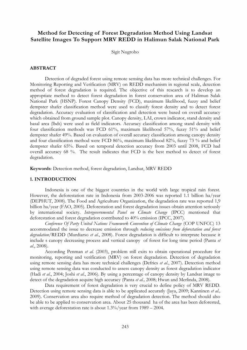
FCD classification was conducted by using FCD-Mapper Ver. 2 software. The detail of classification process can be seen in Figure 2.

245

Figure 2: Forest Canopy Density Classification (Rikimaru, 2003)

Maximum Likelihood Classification

Maximum likelihood classification used training area. The training area was designed by sample which obtain from high resolution image (Qiuckbird image).

Fuzzy Classification

Fuzzy classification consider mixed make-up pixel which can not be defined exactly in one land cover class. This classification require membership function. It is to define what one pixel include some land cover class or another land cover class. Membership function have value from 0 - 1. The value of membership obtained from high resolution image (Qiuckbird image).

Belief Dempster Shafer Classification

Belief classification is classification process to create decision based on degree of belief. The value of degree belief was obtained from confusion matrix among training area and field data. The range of degree belief value is from 0 to 1.

2.2.2 Field Sampling

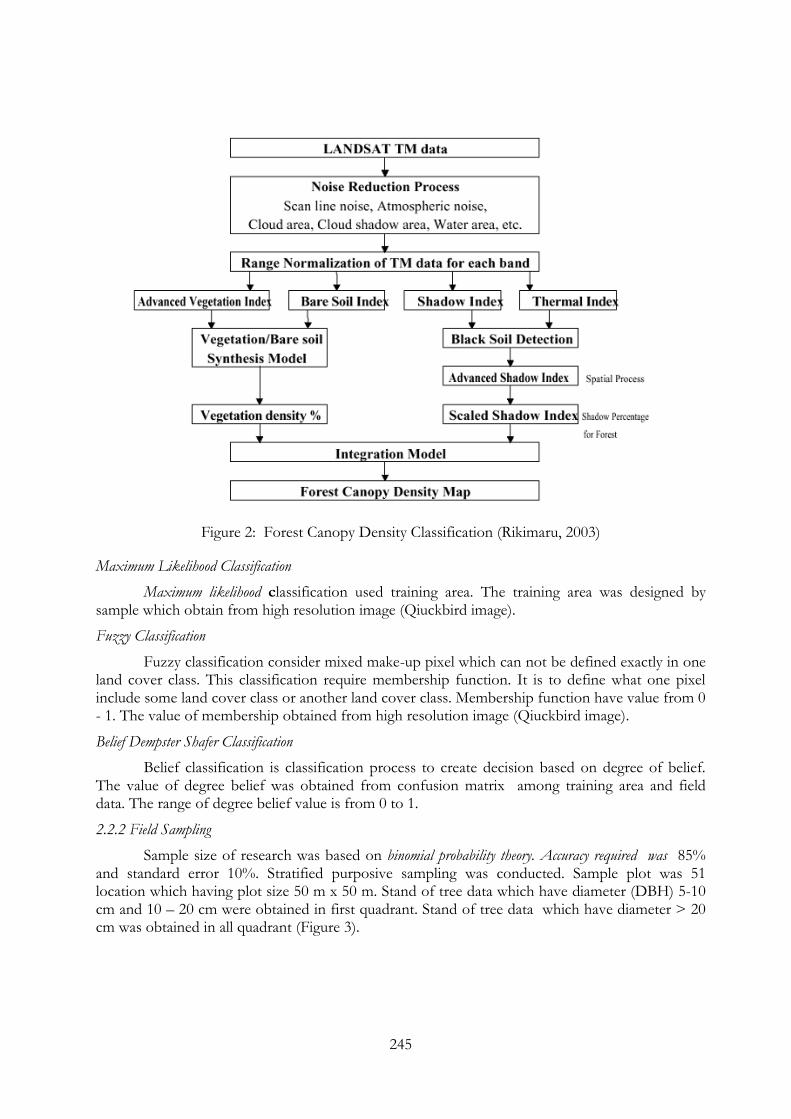
Sample size of research was based on binomial probability theory. Accuracy required was 85% and standard error 10%. Stratified purposive sampling was conducted. Sample plot was 51 location which having plot size 50 m x 50 m. Stand of tree data which have diameter (DBH) 5-10 cm and 10 – 20 cm were obtained in first quadrant. Stand of tree data which have diameter > 20 cm was obtained in all quadrant (Figure 3).

246

Figure 3: Design of sampling plot

2.2.3 Identification of degradation

Criteria to identify degraded forest in the field are decreasing of stand density, basal area, volume, crown indicator dan Leaf Area Index/LAI (Sprintsin et al., 2009; SEAMEO BIOTROP 2001; IPCC, 2009). Leaf Area Index (LAI) is indicator which was used by Global Circulations Models for Predicting Global Warming (Kusakabe et al., 2000).

Regression analysis were conducted to identify degraded forest by each variable. Dependent variables (Y) are stand density (Kt), basal area (lbds) and volume (V). Independent variable (X) are canopy density (Kr), LAI, Crown Size Index (CSI), Crown Damage Index (CDI) dan Visual Crown Rating (VCR).

2.2.4 Evaluation of Accuracy

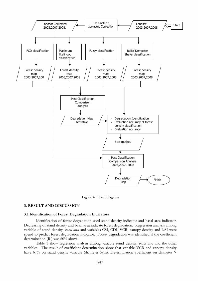
The result of forest density classification was evaluated with canopy density, stand density, crown indicator, LAI and basal area. Evaluation of accuracy use user’s accuracy, producer’s accuracy and overall accuracy and Kappa analysis. Flow diagram of research can be seen in Figure 4. The main step are image processing, data analysis, and reporting the research result. The first step is radiometric and geometric image correction. The second is classifying image using four methods to obtain forest density. The third step is evaluation of accuracy to get the most appropriate method. The last step is analyzing temporal degradation from 2003- 2008 using a post classification comparison method.

10 x10 m

50 m

5 x 5 m

25 x 25 m

50 m

Diameter > 5 – 10 cm

Diameter > 10 - 20 cm

Diameter > 20 cm

Center Plot

I II

III IV

247

Figure 4: Flow Diagram

3. RESULT AND DISCUSSION

3.1 Identification of Forest Degradation Indicators

Identification of forest degradation used stand density indicator and basal area indicator. Decreasing of stand density and basal area indicate forest degradation. Regression analysis among variable of stand density, basal area and variables CSI, CDI, VCR, canopy density and LAI were spend to predict forest degradation indicator. Forest degradation was identified if the coefficient determination (R2) was 60% above.

Table 1 show regression analysis among variable stand density, basal area and the other variables. The result of coefficient determination show that variable VCR and canopy density have 67% on stand density variable (diameter 5cm). Determination coefficient on diameter >

- Degradation Identification - Evaluation accuracy of forest

density classification - Evaluation accuracy

Forest density map

2003,2007,2008

Forest density map

2003,2007,2008

Forest density map

2003,2007,2008

Forest density map

2003,2007,2008

Best method

Post Classification Comparison

Analysis Map 2003,2007, 2008

Degradation Map

Finish

Degradation Map Tentative

Post Classification Comparison Analysis

2003,2007, 2008

Start Landsat Corrected

2003,2007,2008,

Landsat

2003,2007,2008.

Radiometric &

Geometric Correction

Maximum likelihood classification

FCD classification

Fuzzy classification

Belief Dempster

Shafer classification

248

10cm is 62% on variable VCR. Determination coefficient on diameter > 20cm is the highest (80%) on VCR variable.

Table 1. Regression analysis among stand density, basal area and LAI, CSI, CDI, VCR, canopy density.

Coefficient determination (r2)

No Variable Stand density Basal area

Diameter > 5cm

Diameter > 10cm

Diameter > 20cm

Diameter > 5cm

Diameter > 10cm

Diameter > 20cm

1 LAI 0.51 0.38 0.37 0.45 0.41 0.36

2 CSI 0.58 0.58 0.79 0.55 0.53 0.45

3 CDI 0.58 0.57 0.66 0.43 0.39 0.31

4 VCR 0.63 0.62 0.80 0.54 0.51 0.42

5 Canopy Density

0.67 0.49 0.59 0.52 0.46 0.57

Based on regression analysis, the best indicator to predict forest degradation is stand density (diameter 20cm above) using variable canopy density and VCR. The results of regression analysis were used to classify each variable used to examine images classification accuracy. Table 2 show classification of each variable which indicate forest density.

Table 2. Classification of forest density based on stand density, basal area, canopy density, crown indicator and LAI

No Classification

Basal Area m2/Ha

Stand density (N/Ha)

Canopy Density (%)

LAI Crown Indicators /Ha

CSI CDI VCR

1 NH 0 - 2 0-64 0-10 0-0.57 0-1203 0-701 0-1014

2 H1 3- 14 64- 351 11-30 0.59-1.6

1203 -2907

701- 1899

1014-2678

3 H2 15- 25 352-774 31-50 1.7-2.7

2908-4613

1900-3098

2679-4343

4 H3 26-37 775-1304

51-70 2.8-3.7

4614-6317

3099-4296

4344-6007

5 H4 >38 >1305 >71 > 3.8 >6318 >4297 >6008 Note: H4= very high forest density, H3= high forest density, H2= middle forest density, H1= low forest density, NH = Non Forest.

3.2 Identification Rate of Forest Degradation

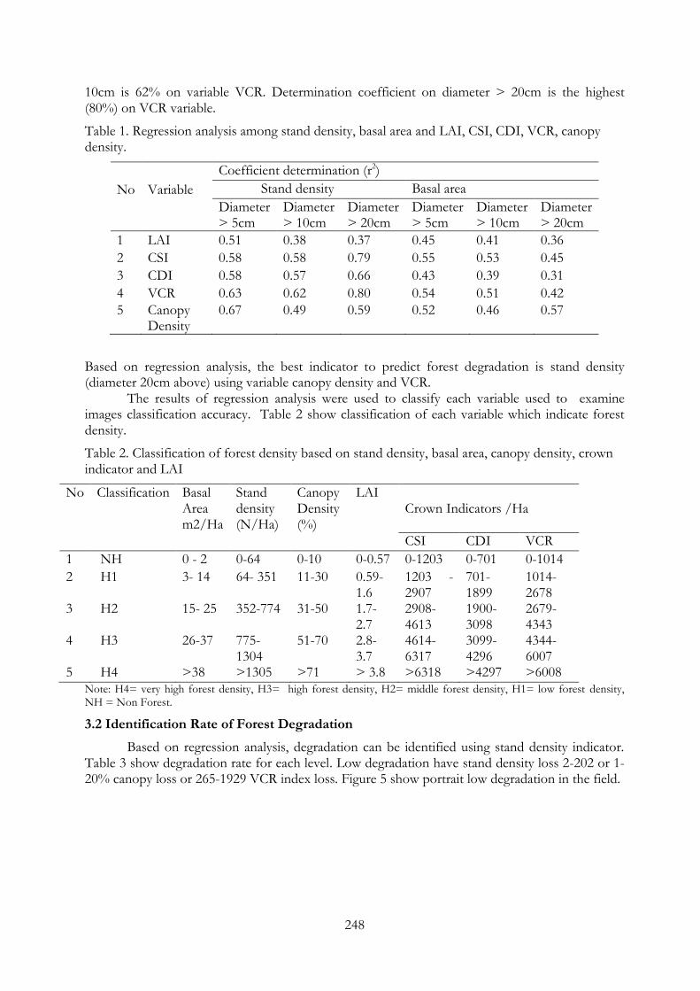
Based on regression analysis, degradation can be identified using stand density indicator. Table 3 show degradation rate for each level. Low degradation have stand density loss 2-202 or 1-20% canopy loss or 265-1929 VCR index loss. Figure 5 show portrait low degradation in the field.

249

Table 3. Classification of forest degradation rate

No degradation rate

Loss

Stand density (N/Ha) > 5cm

Canopy density (%)

VCR /Ha

1 Low 2-201 1-20 265-1929

2 Middle 202-568 21-40 1930-3594

3 High 569-1053 41-60 3595-5258

4 Deforested >1054 >60 >5259

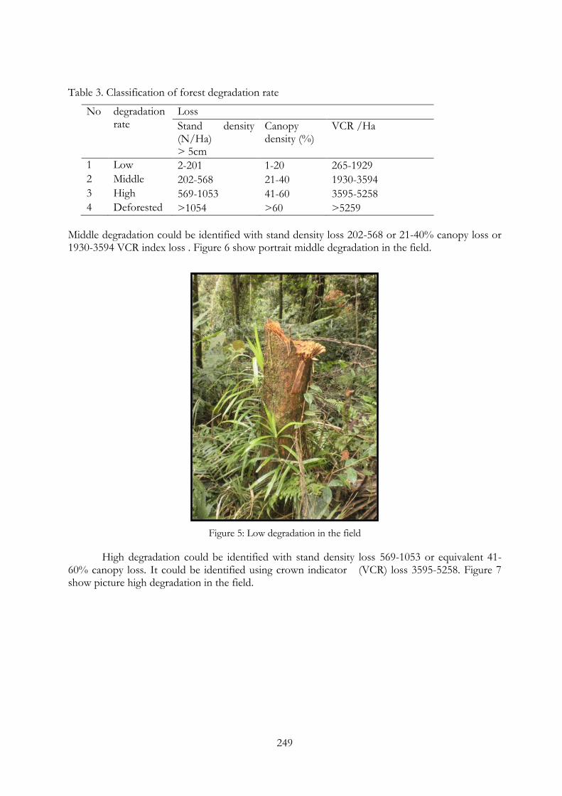
Middle degradation could be identified with stand density loss 202-568 or 21-40% canopy loss or 1930-3594 VCR index loss . Figure 6 show portrait middle degradation in the field.

Figure 5: Low degradation in the field

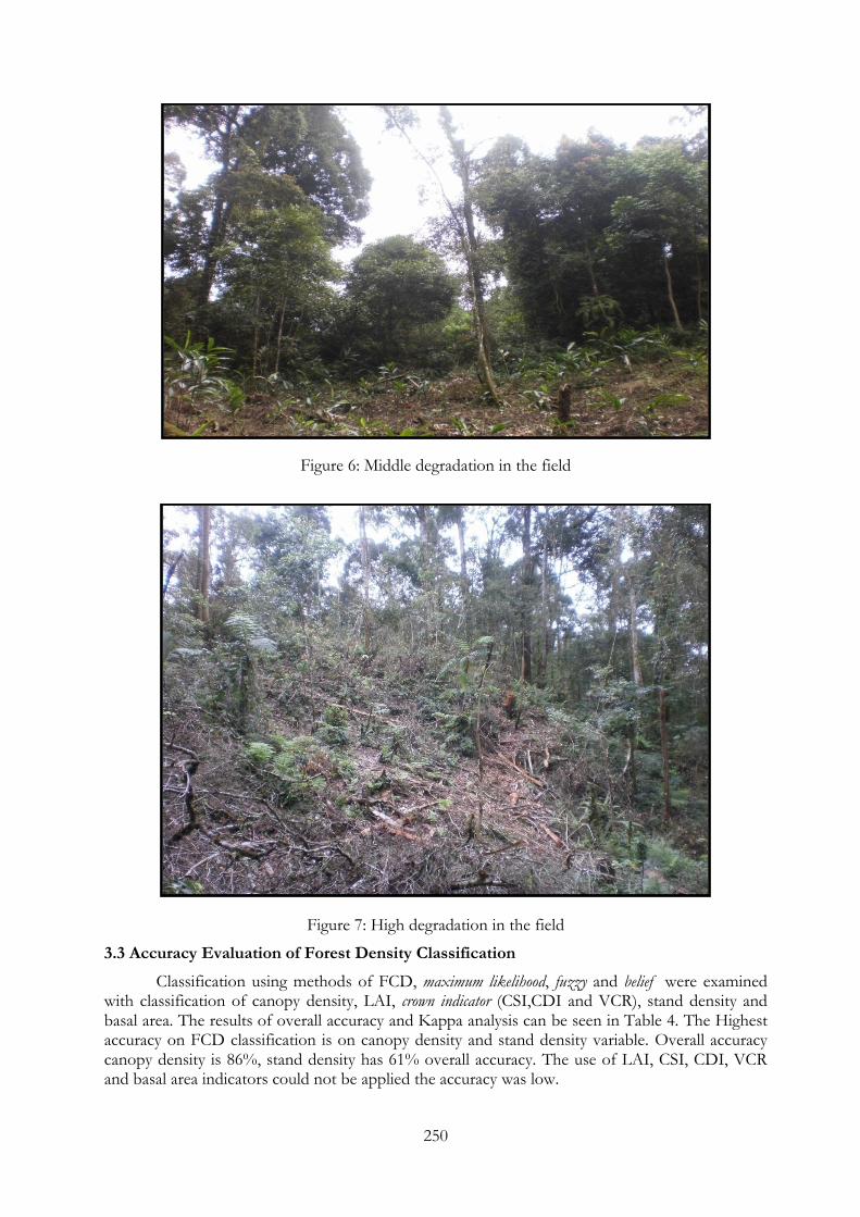
High degradation could be identified with stand density loss 569-1053 or equivalent 41-60% canopy loss. It could be identified using crown indicator (VCR) loss 3595-5258. Figure 7 show picture high degradation in the field.

250

Figure 6: Middle degradation in the field

Figure 7: High degradation in the field

3.3 Accuracy Evaluation of Forest Density Classification

Classification using methods of FCD, maximum likelihood, fuzzy and belief were examined with classification of canopy density, LAI, crown indicator (CSI,CDI and VCR), stand density and basal area. The results of overall accuracy and Kappa analysis can be seen in Table 4. The Highest accuracy on FCD classification is on canopy density and stand density variable. Overall accuracy canopy density is 86%, stand density has 61% overall accuracy. The use of LAI, CSI, CDI, VCR and basal area indicators could not be applied the accuracy was low.

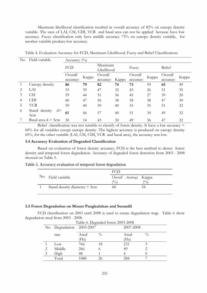
251

Maximum likelihood classification resulted in overall accuracy of 82% on canopy density variable. The uses of LAI, CSI, CDI, VCR and basal area can not be applied because have low accuracy. Fuzzy classification only have middle accuracy 73% on canopy density variable, for another variable produce low accuracy.

Table 4. Evaluation Accuracy for FCD, Maximum Likelihood, Fuzzy and Belief Classifications

No Field variable Accuracy (%)

FCD Maximum Likelihood

Fuzzy Belief

Overall accuracy

Kappa Overall accuracy

Kappa

Overall accuracy

Kappa Overall accuracy

Kappa

1 Canopy density 86 79 82 74 73 59 65 49

2 LAI 53 39 47 32 43 26 51 35

3 CSI 59 44 51 36 45 27 39 20

4 CDI 60 47 56 38 58 38 47 30

5 VCR 59 40 59 40 55 35 51 32

6 Stand density d> 5cm

61 46 57 40 51 34 49 32

7 Basal area d > 5cm 30 14 43 30 49 36 47 32

Belief classification was not suitable to classify of forest density. It have a low accuracy < 60% for all variables except canopy density. The highest accuracy is produced on canopy density 65%, for the other variable (LAI, CSI, CDI, VCR and basal area), the accuracy was low.

3.4 Accuracy Evaluation of Degraded Classification

Based on evaluation of forest density accuracy, FCD is the best method to detect forest density and temporal forest degradation. Accuracy of degraded forest detection from 2003 - 2008 showed on Table 5.

Table 5. Accuracy evaluation of temporal forest degradation

No Field variable

FCD

Overall Accuracy (%)

Kappa (%)

1 Stand density diameter > 5cm

68 54

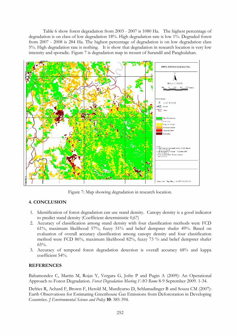
3.5 Forest Degradation on Mount Pangkulahan and Surandil

FCD classification on 2003 until 2008 is used to create degradation map. Table 6 show degradation areal from 2003 - 2008.

Table 6. Degraded forest 2003-2008

No Degradation 2003-2007 2007-2008

rate Areal (Ha)

% Areal (Ha)

%

1 Low 766 18 231 5 2 Middle 266 6 49 2 3 High 48 1 4 0

Total 1080 26 284 7

252

Table 6 show forest degradation from 2003 - 2007 is 1080 Ha. The highest percentage of degradation is on class of low degradation 18%. High degradation rate is low 1%. Degraded forest from 2007 - 2008 is 284 Ha. The highest percentage of degradation is on low degradation class 5%. High degradation rate is nothing. It is show that degradation in research location is very low intensity and sporadic. Figure 7 is degradation map in mount of Surandil and Pangkulahan.

Figure 7: Map showing degradation in research location.

4. CONCLUSION

1. Identification of forest degradation can use stand density. Canopy density is a good indicator to predict stand density (Coefficient deterministic 0,67)

2. Accuracy of classification among stand density with four classification methods were FCD 61%, maximum likelihood 57%, fuzzy 51% and belief dempster shafer 49%. Based on evaluation of overall accuracy classification among canopy density and four classification method were FCD 86%, maximum likelihood 82%, fuzzy 73 % and belief dempster shafer 65%.

3. Accuracy of temporal forest degradation detection is overall accuracy 68% and kappa coefficient 54%.

REFERENCES

Bahamondez C, Martin M, Rojas Y, Vergara G, Jofre P and Pugin A (2009): An Operational Approach to Forest Degradation. Forest Degradation Meeting FAO Rome 8-9 September 2009. 1-34.

Defries R, Achard F, Brown F, Herold M, Murdiyarso D, Schlamadinger B and Souza CM (2007): Earth Observations for Estimating Greenhouse Gas Emissions from Deforestation in Developing Countries. J Environmental Science and Policy 10: 385-394.

253

[DEPHUT] Departemen Kehutanan (2008): Perhitungan Deforestasi Indonesia Tahun 2008. Jakarta: Departemen Kehutanan Republik Indonesia.

[FAO] Food & Agriculture Organization's (2005): Forest Resources Assessment 2005 Update 2005. Terms and Definition. Rome: FRA Programe

Hadi F, Wikantika K and Sumarto I (2004): Implementation of Forest Canopy Density Model to Monitor Forest Fragmentation in Mt. Simpang and Mt. Tilu Nature Reserves, West Java, Indonesia. Indonesian FIG Regional Conference 3-7 Oktober 2004.

Hwan OM and Merlinda R M (2008): Forest Canopy Density Mapping For Forest Climate Change Mitigation/REDD Activities. Japan-Asia REDD Seminar [24-25 March] IPCC] Intergovermental Panel On Climate Change (2007): Fourth Assesment Report:Climate Change. http://www.ipcc-nggip.iges.or.jp/public/2006gl.vol4.html [April 2008].

Jaya I N S (2009): Analisis Citra Digital. Bogor: Fakultas Kehutanan Institut Pertanian Bogor.

Jensen J R (2005): Introductory Digital Image Processing. Third Edition. South California: Pearson Prentice Hall.

Joshi C, Leeuw JD, Skidmorr AK, Duren IC and Oosten H (2006): Remotely Sensed Estimation of Forest Canopy Density: a Comparison of the Performance of Four Methods. Int. J. Applied Earth Observation and Geoinformation 8:84-94.

Kanninen M, Murdiyarso D, Seymour F, Angelsen A, Wunder S and German L (2009): Apakah Hutan dapat Tumbuh di atas Uang. Implikasi penelitian Deforestasi bagi Kebijakan yang Mendukung REDD. Perspektif Kehutanan 4:1-55. Bogor: CIFOR.

Kusakabe T, Tsuzuki H, Hughes G and Sweda T (2000): Extensive Forest Leaf Area Survey Aiming at Detection of Vegetation Change in Subartic-boreal Zone. J Polar Biosci 13:133-146.

Murdiarso D (2008): Measuring and monitoring Forest Degradation for REDD, Implications of Country Circumstances. Bogor. Info Brief Cifor 16.

Panta M, Kim K and Joshi C (2008): Temporal Mapping of Deforestation and Forest Degradation in Nepal: Applications to Forest Conservation. J. Forest Ecology and Management 256:1587-1595.

Penman J, Gytarsky M, Hiraishi T, Krug T, Kruger D, Pipatti R, Buendia L, Miwa K, Ngara T, Tanabe K and Wagner F (2003): Good Practice Guidance for Land Use, Land-Use Change and Forestry. IPCC National Greenhouse Gas Inventories Programme and Institute for Global Environmental Strategies (IGES), Kanagawa, Japan. Intergovernmental Panel on Climate Change. http://www.ipcc-nggip.iges.or.jp/ public/gpglulucf/gpglulucf_contents.htm. [ 3 Maret 2010].

Rikimaru A (2003): Concept of FCD Mapping Model and Semi-Expert System. Japan: Overseas Forestry Consultants Association.

Roy P S (2003): Space Remote Sensing for Forest Management. Dehradun: Indian Institute of Remote Sensing

[SEAMEO BIOTROP] South Asian Regional Center for Tropical Biology (2001): Forest Health Monitoring to he Suistainability of Indonesia Tropical Rain Forest. Bogor: ITTO- SEAMEO BIOTROP.

Sprintsin M, Karnieli A, Sprintsin S, Cohen S and Berliner P (2009): Relationships Between Stand Density and Canopy Structure in a Dryland Forest as Estimated by Ground-based Measurements and Multi-spectral Spaceborne Images. Journal of Arid Environments 73:955–962.

[TNHS] Taman Nasional Halimun Salak 2007. Management Plan Taman Nasional Halimun Salak 2007-2026. Sukabumi: Taman Nasional Halimun Salak.

254

INAFOR 11D-030

INTERNATIONAL CONFERENCE OF INDONESIAN FORESTRY RESEARCHERS (INAFOR)

Section D Forest Assessment and Modelling

Teak Model: A Process-Based Model of Fast Growing Teak Growth and Production

Eliyani

Information Technology, Mercu Buana University Jl. Meruya Selatan no. 1, Jakarta 11650, INDONESIA

Paper prepared for The First International Conference of Indonesian Forestry Researchers (INAFOR)

Bogor, 5 – 7 December 2011

INAFOR SECRETARIAT Sub Division of Dissemination, Publication and Library

FORESTRY RESEARCH AND DEVELOPMENT AGENCY Jl. Gunung Batu 5, Bogor 16610

255

Teak Model: A Process-Based Model of Fast Growing Teak Growth and Production

Eliyani

Information Technology, Mercu Buana University Jl. Meruya Selatan no. 1, Jakarta 11650, INDONESIA

ABSTRACT

Information on growth response of fast growing teak to environment is very limited while the interest to grow this kind of teak is high. Conducting some field experiments to get some information about the response of fast growing teak growth to some environmental variability needs much energy, time and money. Teak model is a software of process-based model that can describe the relationship between fast growing teak growth and soil water availability, therefore, it can simulate the teak growth in some water regimes. The model consists of three sub-models, i.e.: phenology, growth, and soil water balance. The phenology sub model is used to simulate the occurance of new leaves and the associated shoots based on thermal unit concept, while the stage of development determines the biomass to different organs. Tree growth is simulated from biomass production using the approach of light use efficiency, respiration and water availability factor. Water balance sub model, to derive the water availability factor, that consists of input (rainfall and irrigation) and the water loss comprising canopy interception, drainage, soil evaporation and transpiration. Water availability factor is calculated from the computed soil moisture. Some of model parameters were obtained from field experiment. To mimic the response of teak growth in some water regimes, the field experiment was conducted in three levels of irrigation, i.e.: without irrigation, irrigation with 7 mm day-1 and irrigation with 14 mm day-1. Resolution of the model is daily time step which can be run to many years assuming the same weather each year. The model calculates the development and growth of individual tree stand. The results show that the calibrated model describes the dynamics of stem height and diameter.

Keywords: Fast growing teak, process-based model, software

1. INTRODUCTION

In some recent years, teak has been planted in many areas of Indonesia including the areas that would have been considered marginal for teak growing two decades ago. Although teak management has been established through experiences of nearly two centuries, but those experiences are derived from a limited area, especially Java, which has been known as a suitable land for many agricultural systems. The models or allometric equations, which have been built possibly, could not be applied to other regions due to its empirical characteristics.

Process-based models with a high generality can be used to select new plantation sites or assess the risks associated with particular plantation locations or forest management options. The other potential uses of forest growth models as management tools for plantation might include: (1) the prediction of growth and yield from established plantations; (2) selection of species for particular sites; (3) identification of site limitations to productivity; (4) questions for which ‗real-time‘ experiments are not feasible, e.g., long term impact of practices on sustainability or the effects of climate change on forest succession (Battaglia and Sands, 1998).

Teak model is a process-based model which was built to describe the effect of water availability to the growth of fast growing teak, therefore it can simulate the teak growth and production in some water regimes. Water is a limiting factor for the growth of many plants in Indonesia.

256

2. METHODS

There were two separated works in constructing this Teak Model: the field experiment to get some growth paramaters and the model construction.

2.1 Field Experiment

The field experiment was conducted over two years by planting four months old ‗Golden teak‘ seedlings derived from tissue culture. The experimental design was completely randomized block design with three treatments and three replications. The treatments were three levels of irrigation, i.e.: without irrigation, irrigation with 7 mm day-1 and irrigation with 14 mm day-1. The treatments were applied for ten months since one week after planting. The growth parameters obtained by non destructive and destructive method from this field experiment were: Light Use Efficiency, Specific Leaf Area, Wood Density, Extinction Coefficient, Coefficient of maintenance respiration , and Thermal Unit of Leaf emergence and drop.

2.2 Model Construction

The model predicts individual fast growing teak growth on a daily time step. It consists of three sub-models: development, growth, and water balance.

2.2.1 Development Sub-Model

Plant development is described by the occurance of new leaves based on thermal unit concept while the development stage determines the partition of biomass to leaf, stem and root.

2.2.2 Growth Sub-model

Plant growth is derived from biomass production using the approach of light use efficiency, respiration and soil water availability. Dry matter production is proportional to the amount of short wave radiation intercepted by plant canopy (Horie et al., 1995). That relationship applies to tree crops (Sands, 1996). Light use efficiency as a proportionality coefficient has been proved as a convenient basis for empirical production functions in simple model of tree growth. It is customarily defined as increase ε in dry matter production per each unit increase in intercepted radiation (Sands, 1996). The value of ε used in this model was derived from field experiment.

The intercepted radiation by the canopy is calculated using Beer‘s Law (Rosenberg, 1974). The extinction coefficient is assumed to be constant. Its value and the initial value of LAI are derived from field experiment. Specific leaf area is assumed to be constant and the value is also derived from field experiment. The actual production of biomass (B

a) is calculated as a function of

water availability factor (Fw) and potential production of biomass: B

a=FwBb (1)

In this model, we assume that water availability is the only factor limiting the production of biomass. Water factor is a function of relative transpiration (Ta/Tm) (Handoko, 1992). The actual biomass production is partitioned into leaf, stem, and root. The proportion of biomass allocated to organ x is derived from field experiment. A part of the biomass is lost due to maintenance respiration.

As the developmental phase is determined by the occurrence of new leaves with the associated shoot, the partition of biomass into stem and leaf is calculated per internode.

The stem volume of internode i (VS(i)

, m3

) is calculated using:

VS = TW

S/WD (2)

where VS

is stem volume, WS is stem weight and WD is wood density of teak which its value is

derived from field experiment and is assumed to be constant from the bottom to the top.

257

Stem height (H, m) is calculated as:

H = ΣH(i)

(3)

where H(i)

is the height of internode i. The stem diameter (D(i), cm) is calculated using the volume

equation of a cylinder:

2.2.3. The Water Balance Sub-Model

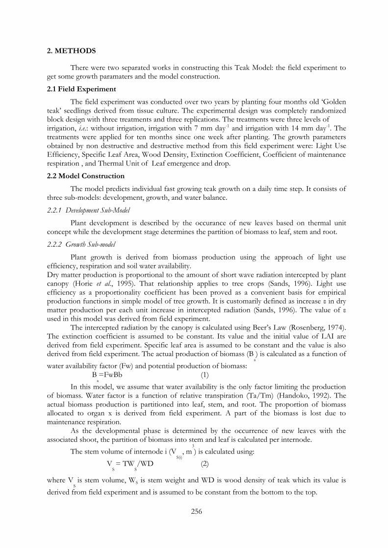
The water balance sub-model is to derive a water availability factor, which is calculated from computed soil moisture. Soil moisture is affected by inputs (rainfall and irrigation) and water loss comprising canopy interception, run-off, drainage, evaporation and transpiration. Figure 1 shows the algorithm of water balance sub model. The tree crown intercepts a part of the rainfall and all of this interception (I

c) will be evaporated. The values of I

c were determined by

Zinke (1967) as a function of leaf area index (LAI) and rainfall (P).

Figure 1: Water balance sub-model

The rest of the rainfall will reach the soil surface as stem flow and throughfall (Sftf). When evaporation = 0 and if soil water content in the first layer (θ1) is more than field capacity of that layer (Fc(1)) or if Sftf is more than extractable water (EW), i.e. available water between wilting point (θwp(1)) and field capacity, run-off (Ro) will take place. The rest of Sftf and irrigation (Ir) is absorbed as infiltration (I

s).

In the model, we assumed that soil is divided into two layers. Percolation (Pc) will take place from each soil layer when soil water content of the layer m (θm) is higher than the field capacity (Fcm). The soil water percolation from the lowest layer is lost as drainage. The other losses of water are

ETm

Tm Em

Qn RH/VPD T u [Lai]

Sf+Tf

[Pwp1] Tr1

Ro

Ic

1

[Fc1]

[Fc2]

Pc1

P

SfTf

Ea Ea Ta

Tr2 [Pwp2]

2

Pc2

Remarks: Lai=leaf area index, ETm=maximum evapotranspiration, Qs=solar radiation, RH=relative humidity, VPD=vapor pressure deficit, Em=maximum evaporation, Tm=maximum transpiration, Ea=actual evaporation,

Ta=actual transpiration, P=precipitation, SfTf=stem flow through fall, 1,2=soil water content in layer 1 and 2, Pc1,2= percolation from layer 1 and 2, Fc1,2=field capacity of layer 1 and 2, Pwp1,2=permanent wilting point of layer 1 and 2, Tr1,2=root transpiration from layer 1 and 2, Ic=canopy interception, Ro=run off.

258

from evapotranspiration. The maximum evapotranspiration (ETm) was assumed to be 80% of the potential evapotranspiration (ETp), which is calculated using the equation from Penman (1948). The maximum soil evaporation and the maximum transpiration are approximated from maximum evapotranspiration assuming that proportion of radiation intercepted by crop canopy equals Tm/ETm (Stapper, 1984; Rimmington and Connor, 1987) in (Handoko, 1992). The actual evaporation (Ea) is calculated using the two-stage soil evaporation of (Ritchie, 1972). To calculate the actual transpiration, it is assumed that roots will absorb the water firstly from the most upper layer, then the next layer until Ta = Tm or until the root depth limit has been reached (Handoko, 1992).

The model assumes that plants are free of pests and diseases, and the water stress does not kill plants. Furthermore, the rate of plant growth is assumed to be uniform so that production per hectare can be predicted from the individual plant production multiplied by plant density. The model can be run for several years. Model inputs are weather variables (radiation, temperature, relative humidity, wind speed and rainfall), soil properties (texture, field capacity, and permanent wilting point) and management (projected area, population per hectare, planting date, and irrigation). Model outputs can be various variables from each sub-model such as biomass, stem height and diameter, stem volume, leaf area index, and carbon content. The program was written using Visual Basic version 6.0.

3. RESULT AND DISCUSSION

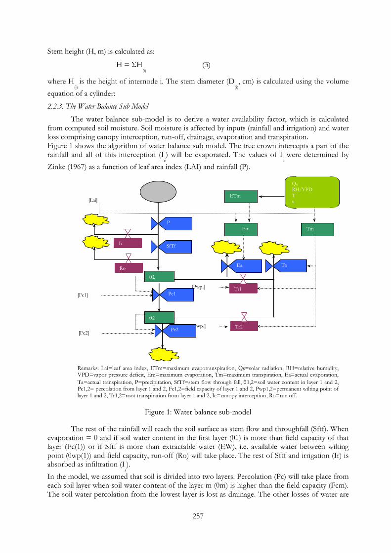
3.1 User Interface

Teak Model consists of four user interfaces : Opening Page, Model Description, Model Input and Model Output. The Opening Page is presented in Figure 2, the interface of Model Description in Figure 3, the Model Input in Figure 4, and the Model Output in Figure 5. To run this software, the user does not need to log in.

Figure 2: The user interface of Opening Page

259

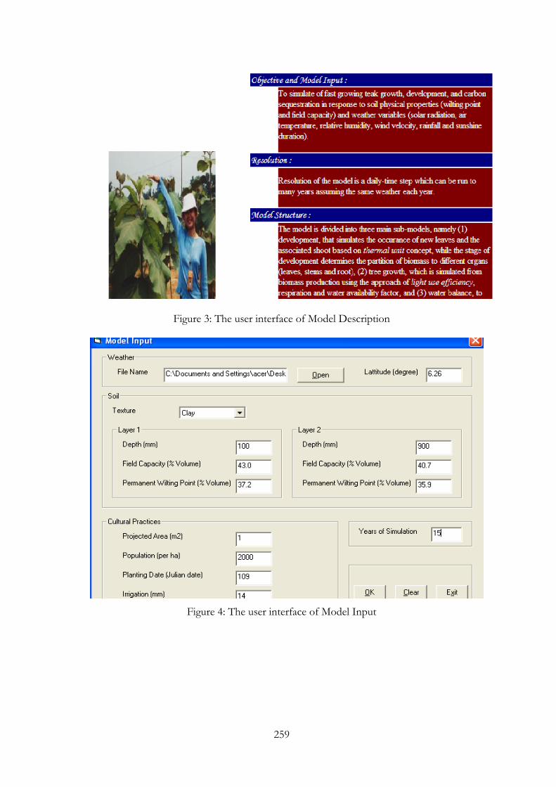
Figure 3: The user interface of Model Description

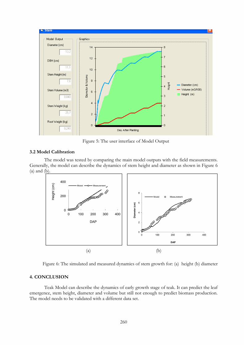
Figure 4: The user interface of Model Input

260

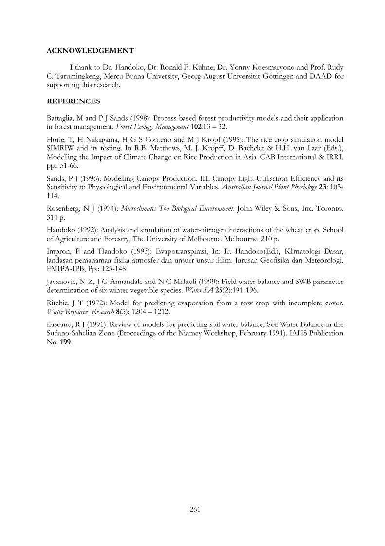
Figure 5: The user interface of Model Output

3.2 Model Calibration

The model was tested by comparing the main model outputs with the field measurements. Generally, the model can describe the dynamics of stem height and diameter as shown in Figure 6 (a) and (b).

(a) (b)

Figure 6: The simulated and measured dynamics of stem growth for: (a) height (b) diameter

4. CONCLUSION

Teak Model can describe the dynamics of early growth stage of teak. It can predict the leaf emergence, stem height, diameter and volume but still not enough to predict biomass production. The model needs to be validated with a different data set.

261

ACKNOWLEDGEMENT

I thank to Dr. Handoko, Dr. Ronald F. Kühne, Dr. Yonny Koesmaryono and Prof. Rudy C. Tarumingkeng, Mercu Buana University, Georg-August Universität Göttingen and DAAD for supporting this research.

REFERENCES

Battaglia, M and P J Sands (1998): Process-based forest productivity models and their application in forest management. Forest Ecology Management 102:13 – 32.

Horie, T, H Nakagama, H G S Conteno and M J Kropf (1995): The rice crop simulation model SIMRIW and its testing. In R.B. Matthews, M. J. Kropff, D. Bachelet & H.H. van Laar (Eds.), Modelling the Impact of Climate Change on Rice Production in Asia. CAB International & IRRI. pp.: 51-66.

Sands, P J (1996): Modelling Canopy Production, III. Canopy Light-Utilisation Efficiency and its Sensitivity to Physiological and Environmental Variables. Australian Journal Plant Physiology 23: 103-114.

Rosenberg, N J (1974): Microclimate: The Biological Environment. John Wiley & Sons, Inc. Toronto. 314 p.

Handoko (1992): Analysis and simulation of water-nitrogen interactions of the wheat crop. School of Agriculture and Forestry, The University of Melbourne. Melbourne. 210 p.

Impron, P and Handoko (1993): Evapotranspirasi, In: Ir. Handoko(Ed.), Klimatologi Dasar, landasan pemahaman fisika atmosfer dan unsurr-unsur iklim. Jurusan Geofisika dan Meteorologi, FMIPA-IPB, Pp.: 123-148

Javanovic, N Z, J G Annandale and N C Mhlauli (1999): Field water balance and SWB parameter determination of six winter vegetable species. Water SA 25(2):191-196.

Ritchie, J T (1972): Model for predicting evaporation from a row crop with incomplete cover. Water Resources Research 8(5): 1204 – 1212.

Lascano, R J (1991): Review of models for predicting soil water balance, Soil Water Balance in the Sudano-Sahelian Zone (Proceedings of the Niamey Workshop, February 1991). IAHS Publication No. 199.

262

INAFOR 11D-031

INTERNATIONAL CONFERENCE OF INDONESIAN FORESTRY RESEARCHERS (INAFOR)

Section D Forest Assessment and Modelling

Expansion Factors for Estimating Biomass of Logged Over Tropical Rain Forest in Central Kalimantan

Baroroh Wista Anggraeni1, Ris Hadi Purwanto2 and Ronggo Sadono2

1Faculty of Forestry, Muhammadiyah University Jl. Pasir Kandang No.4 Padang, West Sumatera, INDONESIA

Corresponding email: bw.anggraeni@yahoo.com

2,3

Faculty of Forestry, Gadjah Mada University

Jl. Agro-Bulaksumur, Yogyakarta 55281, INDONESIA

Paper prepared for The First International Conference of Indonesian Forestry Researchers (INAFOR)

Bogor, 5 – 7 December 2011

INAFOR SECRETARIAT Sub Division of Dissemination, Publication and Library

FORESTRY RESEARCH AND DEVELOPMENT AGENCY Jl. Gunung Batu 5, Bogor 16610

263

Expansion Factors for Estimating Biomass of Logged Over Tropical Rain Forest in Central Kalimantan

Baroroh Wista Anggraeni1, Ris Hadi Purwanto2 and Ronggo Sadono2

1Faculty of Forestry, Muhammadiyah University Jl. Pasir Kandang No.4 Padang, West Sumatera, INDONESIA

Corresponding email: bw.anggraeni@yahoo.com

2,3Faculty of Forestry, Gadjah Mada University

Jl. Agro-Bulaksumur, Yogyakarta 55281, INDONESIA

ABSTRACT

Stem and merchantable wood volume are common variables in forestry. Furthermore, The information of total biomass in tropical rainforests is an important variable for ecologists, biogeochemists, foresters and policymakers. To make better inferences on long-term changes in total biomass, it is essential to know the model associated with total biomass estimation. In this research, we develop model for predicting total biomass of forests in PT Sari Bumi Kusuma (PT SBK), Central Kalimantan, called scaling factors. Scaling factors consist of Brushwood Factor (Ebr), Leaf Factor (El), and Root Factor (Er) that are values of thumb for converting wood volume to wood biomass and total tree biomass. Destructive sampling was used to collect the samples. In total 40 trees with dbhs ranging from 1.1 to 115 cm. Tree samples were 23 and 17, originally classified as forest with line planting system and TPTI system, respectively. Scaling factors for Ebr, El, and Er are 1.46; 1.21; 1.25 for forest with line planting. The Ebr, El, and Er for forest with TPTI system are 1.27; 1.11; 1.16, respectively. The factors provide a rough estimate of standing total biomass in relation to standing merchantable volume. Scaling factors are used in the step-by-step conversion of merchantable volume to aboveground and belowground. The factors Ebr, El and Er are used to determine the proportion of branch wood, the foliage mass and the root biomass respectively. The research findings are new for alternative model to facilitate the approximate conversion of known forestry parameters to total biomass in Indonesia.

Keywords: Conversion models, merchantable wood volume, total biomass.

1. INTRODUCTION

Tropical rainforests are recognised worldwide for their high biodiversity and also for the role they play in flood amelioration, soil conservation, carbon storage, and for their influence on climate (Laurance, 1999). Tropical forests are, on average, the most productive of all natural ecosystems and cycle the largest amounts of nutrients (Abe, 2007). The coverage of natural forest is decreasing very rapidly, however, due to poor concession management, illegal logging, forest fires and land use conversion (Kangas et al., 2006).

The forest ecosystem is an important carbon sink and source containing majority of the above ground terrestrial organic carbon, yet uncertainty remains regarding their quantitative contribution to the global carbon cycle. On the oter hand, forest degradation and deforestation caused decrease the carrying capacity of tropical forests in maintaining ecological systems. The ecological systems of tropical forest are dynamic, so the ability of forests to absorb carbon is increasingly limited because forest ecosystem plays very important role in the global carbon cycle and they have the potential to assimilate and store relatively large fractions of carbon. Nevertheless, tropical deforestation in many parts of the world continues at an alarming rate. Tropical forests are a particular concern because they are undergoing significant change, and there are few reliable biomass estimates for these forests (Brown, 1997).

264

The estimation of aboveground biomass is an essential tool for evaluating the productivity and nutrient cycling of forests. To assess the role of forests as carbon sinks and sources, an accurate means of estimating forest biomass must be developed. The biomass dynamics of secondary forests are of special interest, because such forests are spreading rapidly as a result of forest degradation in the tropics. For these reasons, we need an efficient and accurate means of biomass estimation. With biomass estimations the magnitude of the sources and sinks in these forests can be evaluated and the role of secondary tropical forests in the global carbon cycle will be better understood.

Aboveground biomass can be measured with two common methods. Weighing tree biomass in the field is the most accurate approach, but is destructive and laborious, and is thus generally limited to small areas. In contrast, a method using model for estimation of biomass is more cost-effective. Moreover, well developed model can estimate forest biomass of other stands easily and non-destructively. Therefore, accurate methods for estimating aboveground biomass in logged-over tropical rainforest are needed to estimate the effects of carbon sequestration after logging and to evaluate the baseline for nations carbon storage on the REDD scheme (Gibbs et al., 2007).

Tropical rain forests of South-East Asia have potentially larger biomasses than other tropical forest ecosystems (Brown et al.,1989). Biomass estimation of tropical rain forests in South East Asia has been carried out intensively in Malaysia and Indonesia (Yamakura et al.,1986; Ketterings et al., 2001; Hashimoto et al., 2004; Basuki et al., 2009; Kenzo et al., 2009a). However, most of these previous studies assessed only above-ground biomass. Few exceptions (Kenzo et al., 2009b; Niiyama et al.,2010) have rarely examined root mass at the individual tree level. The lack of knowledge concerning belowground total biomass remains common to tropical rain forests worldwide (Chave et al., 2005) especially for larger trees. Thus, there is a need for a reliable method for estimating root biomass to quantify carbon balances in tropical rain-forest ecosystems.

One of forest concession area in Central Kalimantan is PT. Sari Bumi Kusuma (PT SBK). PT. SBK is located in south west of the National Park (TN) Bukit Baka-Bukit Raya, so the forest types were similar in forest biodiversity, especially trees (Soekotjo, 2009). Estimation of biomass is an important aspect of studies of forest productivity at PT SBK. Knowledge of the biomass and carbon in these forests is critical to establishing sustainable forest management strategies, both in order for assest the impact of logging and the global carbon cycle. Chave et al. (2004) explained that one of the large sources of uncertainty in all estimates of carbon stocks in tropical forests is the lack of standard models for converting tree measurements to aboveground biomass. Therefore, it is important to develop models for estimating biomass in the tropical forests area. Here, we were to develop model for estimating biomass of the forest in PT SBK, called scaling factor.

2. EXPERIMENTAL METHODS

2.1 Research Site

The study area is located within the forest concession area of PT SBK and it was conducted from July till August 2010. While laboratory analysis conducted in November 2010 to June 2011.

2.2 Data Collecting Method

Forest biomass estimation involved two phases. In the first is the destructive harvesting of trees and the second is analyzing in the laboratory. The study sites were originally classified as forest with the line planting system and forest with TPTI system that have been selectively logged. The tree sizes selected were based on an even distribution in the DBH, starting from DBH=1.1 cm up to DBH of 115 cm. A number of sample trees smaller than 10 cm DBH were also included to fine tune the trend line at smaller DBH.

265

Initially, during fieldwork, forty trees were destructively measured. They were divided in to 23 trees that representing forest with the line planting system and 17 trees were representing forest with TPTI system. They were harvested and measured for aboveground parts just before root excavation at the sites. Root excavation was carried out for all trees. After harvesting, trees were divided into leaves, branches and main stems in the field (BS). Total fresh weight of each tree part was measured in the field (BBS).

The destructive method is done by felling the sample tree and then weighing it. Direct weighing can only be done for small trees, but for larger trees, partitioning is necessary so that the partitions can fit into the weighing scale. In cases where the tree is large, volume of the stem is measured. Sub-samples are collected, and its fresh weight, dry weight, and volume are measured. The dry weight of the tree (biomass) is calculated based from the ratio of fresh weight (or volume) to the dry weight.

In the second stage, conducted in the laboratory, representative samples were dried in the laboratory to determine moisture content. For volume determination, wood samples were saturated with water, and then the volume was measured by water displacement (Chave, 2005). The wood and leaf samples were also oven-dried at 103 ± 2˚C until constant weight (BK).

2.3 Data Analysis Method

2.3.1 Biomass of Trees

The content of the biomass of each organ of trees, stem, branches and twigs, leaves, and roots according to Jarayaman (1999) in Samalca (2007) are:

BBSBS

BKB

Total biomass / total weight (Wt) is

Wt = total biomass Ws = stem biomass Wb = branch biomass Wl = leaves biomass Wr = root biomass

2.3.2 Developing Models

In addition to stem wood, the aboveground wood volume also includes brushwood (Pretzsch, 2009). Therefore the factor of brushwood (non merchantable wood, including the branches and wigs) can be used to calculate the difference between total aboveground biomass and the merchantable biomass. Expansion factors branches or twigs (Ebr) that presented by Pretzsch (2009) are:

Wwag

Ebr =

Wm

Wwag is the total aboveground woody biomass and Wm is the merchantable biomass. Pretzsch (2009) describes the brushwood is wood of branches and twigs. On the other hand, the mean of merchantable wood in Indonesia is different from Pretzsch (2009), here, we define brushwood is non merchantable wood including stem, branch, and twig, that become waste in

Wt = Ws + Wb + WL + Wr

(1)

(2)

(3)

266

harvesting process in tropical forests. While the biomass of merchantable wood is limited to trunk that free from branches, we called Tbbc. Pretzsch (2009) describe that leaf biomass is modelled as a function of aboveground woody biomass. While leaf factor (El) are :

Wag

El =

Wwag Wag is the total aboveground biomass and Wwag are aboveground wood biomass. Wag is the sum of stem, branch / twig, and leaf biomass. Wwag is the sum of stem and branches / twigs biomass without leaf. Santantonio et al. (1977) in Pretzsch (2009) found that the percentage of roots in the total tree biomass range from 10–45% approximately depending on the growth conditions, corresponding to a root factor Er of total biomass. Therefore, Pretzsch (2009) propose the root factor (Er) :

Wt

Er =

Wag Wt is the total biomass is the sum of stem, branch, leaf, and root biomass. Wag is the total aboveground biomass that is the sum of stem, branch, and leaf biomass. The expansion factor of Ebr, El, and Er is used gradually to convert the merchantable volume into above and belowgrond biomass into total biomass. These factors are also used to determine the proportion of branch, leaf, and root biomass to total tree biomass. These factor of branch, leaf, and root (Ebr, El, and Er) by Pretzsch (2009) called the scaling factor are used for the direct conversion of merchantable wood volume or biomass to total tree biomass. Its steps are:

1. Merchantable biomass is multiplied by the brushwood factor (Ebr) to obtain aboveground total woody biomass (stem and branch) respectively.

2. Aboveground total woody biomass is multiplied by the leaf factor (El) to obtain aboveground total biomass.

3. Aboveground total biomass is multiplied by the Er to obtain total tree biomass.

3. RESULT AND DISCUSSION

Forests are open systems. They exchange matter, energy, and genetic information with their environment. Therefore, to understand the system and to model and predict its responses, one must consider the external determinants of growth (precipitation, temperature, radiation, CO2 concentrations, atmospheric deposition etc.) (Pretzsch, 2009). In fact, forest is sink and store carbon in stand biomass. Measurement of carbon stored can be estimated through the forest biomass. Forest biomass can be estimated through direct measurements by destructive methods or based on model that predicts biomass estimated.

Ideally, each species should have its own biomass model, based on a large sample size. But, this was unrealistic for tropical rain forests. It required a method for measuring forest to develop models for estimating biomass. The expected results can be compared between the land and sites that have similar ecosystem in a wider regional scale. Prediction models are important for the sustainability of forest management because Indonesia has a wide range of land uses. It is necessary for validation of model accuracy by comparing model predictions with the reality condition of the stand. Existing models for estimation of biomass is on allometric and biomass expansion factors.

(4)

(5)

267

Models for biomass estimation in tropical forest are constructed from limited samples (Chave et al., 2004). To prepare data for developing model from limited samples, we selected trees from two management systems that representing conditions of the forest ecosystem in PT. SBK. It classified to 23 trees from the forest in line planting with TPTII system and 17 trees from the forest with TPTI system that have been selectively logged.

Beside allometric model and the model biomass expansion factor (BEF) (Brown et al., 1989), scaling factor (Pretzsch, 2009) also proposed as a model to estimate total biomass. In developing the expansion factor of brushwood, leaf, and root obtained Ebr, El, and Er values were 1.27, 1.11, and 1.16 for forest that have been selectively logged, respectively. On the line planting forest Ebr, El, and Er values were, 1.46, 1.21, 1.25, respectively. The orientation value of Ebr, El, and Er serve as a good estimation for broadleaves stand in Europe are described in Pretzsch (2009) 1.5, 1.05, and 1.25, respectively. Ebr factors, ranging from 2 up to 1.2 for young trees to old growth trees. In young stands Ebr is greater because the proportion of merchantable timber on aboveground woody organs is smaller than the old growth stand. The results of this study also showed a similar trend, it was 1.27 for forest that have been selectively logged and 1.46 on the line planting forest.

Leaves factors, El, decreases slightly in line with increases age of the stand slightly. The opinions by Pretzsch (2009) the first approach, leaf biomass is modelled as a function of aboveground woody biomass. In a second approach, the estimate of leaf biomass is independent of wood biomass. Assuming a constant assimilation surface and weight of the leaves in old and uneven-aged stands, the leaf biomass can be estimated from the annual litter fall and the average length of leaf life. The results of this study showed the value of El were 1.1 and 1.21 for forest that have been selectively logged and the line planting forest, respectively. In contrast to the estimated El by Pretzsch (2009) in Europe, for broad-leaved forest in early to mature stands is 1.05.

Santantonio et al., (1977) in Pretzsch (2009) explains that the percentage of roots in the total tree biomass ranges from 10–45% approximately depending on the growth conditions. By Pretzsch (2009) this percentage is called the root factor Er ranged between 1.11 - 1.81. It increases El slightly and the percentage of root to total tree biomass also increases. The Er obtained on this study was 1.16 and 1.25 for forest that have been selectively logged and the line planting forest, respectively. The values are still within the expected range on Pretzsch (2009). The expansion factor Ebr, El, and Er that called a scaling factor, they are used gradually to convert the merchantable volume into total treebiomass. The steps are :

1. Merchantable wood volume(m3) is multiplied by wood density (kg/m3) is converted to merchantable stem biomass (Wm in kg). Wm = V x ρ

2. Merchantable stem biomass (Wm) is multiplied by the brushwood factor (Ebr) to obtain aboveground total woody biomass (Wwag, stem and branch) respectively. Wwag = Wm x Ebr

3. Aboveground total woody biomass (Wwag) is multiplied by the leaf factor (El) to obtain aboveground total biomass(Wag). Wag = Wwag x El

4. Aboveground total biomass (Wag) is multiplied by the Er to obtain total tree biomass. Wt = Wag x Er It is clear if the available of data of Dbh and wood density, estimating total biomass can be

done through factors Ebr, El, and Er. Therefore, the data base in forest management is much needed for accuracy estimates of total biomass. There are some model for estimating total biomass, besides allometric equation and biomass expantion factor, in this study produces three types of models, called scaling factor. They have the same purpose, to make an assessment of total biomass without directly destructive measurements in the field. Choosing the use model depend on the user, which model more effectif is depending on the use of the model.

268

4. CONCLUSION AND RECOMMENDATION

4.1 Conclusion

The model of scaling factor Ebr, El, and Er are 1.27, 1.11, 1.16 for forest that have been selectively logged and forest in line planting 1.46, 1.21, and 1.25, respectively. The factors are used in the step-by-step conversion of merchantable volume to total biomass.

4.2 Recommendations

1. The number of sample trees for developing models may be not enough to represent the species present at the study areas, it is recommended to add sample to improve the results of this study, because the majority of samples had a diameter of less than 100 cm, there were only a tree with a diameter of more than 100 cm. Ideally, there should be several trees which have diameter more than 100 cm for developing mixed species model.

2. Therefore, when choosing biomass estimation model for assessment of the total biomass, it is important to carefully consider their suitability the use of practicality of the model based on the specific intended use of the model.

ACKNOWLEDGEMENT

We would like to express our appreciation to the anonymous reviewers for their

constructive comments on the manuscript. This work is supported by a grant from the Indonesia

Managing Higher Education for Relevance and Efficiency (IMHERE) Faculty of Forestry Universitas Gadjah Mada.

REFERENCES

Abe, H (2007): Forest Management Impacts on Growth, Diversity and Nutrient Cycling of Lowland Tropical Rainforest and plantations, Papua New Guinea. Thesis for the degree of doctor of philosophy of the University of Western Australia School of Plant Biology.

Basuki, T M, P E van Laake, A K Skidmore, Y A Hussin (2009): Allometric Equations for Estimating the Above-ground Biomass in Tropical Lowland Dipterocarp Forest. Forest Ecology and Management 257:1684-1694.

Chave, J, R Condit, S Aguilar, A Hernandez, S Lao and R Perez (2004): Error Propagation And Scaling For Tropical Forest Biomass Estimates. Royal Society 359:409-420.

Chave, J, C Andalo, S Brown, M A Cairns, J Q Chambers, D Eamus, F H Fölster, F Fromard, N Higuchi, J P Lescure, B W Nelson, H Ogawa, H Puig, B Riera and T Yamakura (2005): Tree allometry and improved estimation of carbon stocks and balance in tropical forests. Oecologia 145:87–99.

Kangas, A and M Maltamo (2006): Forest Inventory Methodology and Applications. Springer. Belanda.

Kenzo, T, R Furutani, D Hattori, J J Kendawang, S Tanaka, K Sakurai and I Ninomiya (2009a): Allometric equations for accurate of above-ground biomass in logged-over tropical rainforest in Sarawak, Malaysia, The Japanese Forest Society 14:365–372.

Kenzo, T, T Ichie, D Hattori, T Itioka, C Handa, T Ohkubo, J J Kendawang, M Nakamura, M Sakaguchi, N Takahashi, M Okamoto, A Tanaka Oda, K Sakurai and I Ninomiya (2009b): Development Of Allometric Relationships For Accurate Estimation Of Above- And Below-Ground Biomass In Tropical Secondary Forests In Sarawak, Malaysia. Journal of Tropical Ecology 25:371–386.

269

Laurance, W F (1999): Reflection on the Tropical Deforestation Crisis. Biological Conservation 91: 109-117.

Niiyama, K, T Kajimoto, Y Matsuura, T Yamashita, N Matsuo, Y Yashiro, A Ripin, A R Kassim and N S Noor (2010): Estimation Of Root Biomass Based On Excavation Of Individual Root Systems In A Primary Dipterocarp Forest In Pasoh Forest Reserve, Peninsular Malaysia. Journal of Tropical Ecology 26:271–284.

Pretzsch, H (2009): Forest Dynamics, Growth and Yield. Springer. Berlin.

Samalca, I (2007): Estimation of forest biomass and its error: A case in Kalimantan, Indonesia. MSc thesis, ITC, Enschede

Soekotjo (2009): Teknik Silvikultur Intensif. Gadjah Mada University Press. Yogyakarta

Yamakura, T, Hagihara, A, Sukardjo, S and Ogawa, H (1986): Aboveground Biomass of Tropical Rainforest Stands in Indonesian Borneo. Plant Ecology 68(2):71-82.