METAL ION COMPLEXING AND FLUORESCENCE ... Calculations – Fluoride Affinity 32 Molecular Mechanics Calculations-Chelate Ring Size 33 Molecular Mechanics Calculations-Ideal Ionic Radius

METAL ION COMPLEXING AND FLUORESCENCE PROPERTIES OF THE NOVEL HEMICYCLE, DIPYRIDOACRIDINE, WITH COMPUTATIONAL STUDIES

ON METAL ION SELECTIVITY

Jason Roland Whitehead

A Thesis Submitted to the University of North Carolina Wilmington in Partial Fulfillment

Of the Requirements for the Degree of Master of Science

Department of Chemistry

University of North Carolina Wilmington

2007

Approved by

Advisory Committee

_________________________________ _________________________________

_________________________________ Chair

Accepted by

_________________________________ Dean, Graduate School

TABLE OF CONTENTS

ABSTRACT.........................................................................................................................v

ACKNOWLEDGMENTS ................................................................................................. vi

DEDICATION.................................................................................................................. vii

LIST OF TABLES........................................................................................................... viii

LIST OF FIGURES ........................................................................................................... ix

INTRODUCTION ...............................................................................................................1

Ligands for Biomedical and Sensor Applications ..........................................................1

Ligand Design Rules.......................................................................................................4

Rule 1: Chelate Ring Size Theory .................................................................................4

Rule 2: Hard and Soft Acid-Base (HSAB) Theory........................................................9

Rule 3: Hemicycles and Preorganization Theory ........................................................12

Introduction to 3D Fluorescence...................................................................................15

EXPERIMENTAL METHODS.........................................................................................17

Cleaning of Glassware ..................................................................................................17

Equipment .....................................................................................................................17

Preparation of DPA Solutions.......................................................................................18

Preparation of Metal Solutions .....................................................................................22

UV/Vis Spectrophotometry ..........................................................................................23

Calculations for Titration Data .....................................................................................25

3D Fluorescence Method ..............................................................................................29

COMPUTATIONAL METHODS.....................................................................................31

DFT Calculations ..........................................................................................................31

ii

DFT Calculations – Fluoride Affinity...........................................................................32

Molecular Mechanics Calculations-Chelate Ring Size.................................................33

Molecular Mechanics Calculations-Ideal Ionic Radius and M-N Bond Length...........34

RESULTS AND DISCUSSION........................................................................................36

UV/Vis Spectrophotometry – pKa Determinations ......................................................36

UV/Vis Spectrophotometry – Formation Constant Determination ..............................38

Sodium ..........................................................................................................................40

Calcium.........................................................................................................................44

Mercury.........................................................................................................................47

Lanthanum ....................................................................................................................51

Manganese ....................................................................................................................55

Zinc ...............................................................................................................................59

Indium...........................................................................................................................63

Lutetium........................................................................................................................66

Gadolinium ...................................................................................................................70

Strontium.......................................................................................................................74

3D Fluorescence............................................................................................................78

COMPUTATIONAL RESULTS AND DISCUSSION ....................................................92

DFT Calculations - Fluoride Affinity ...........................................................................92

Molecular Mechanics Calculations – Chelate Ring Size..............................................96

Molecular Mechanics Calculations- Ideal Metal-N Bond Length................................98

Molecular Mechanics Calculations- Ideal Metal Ionic Radius...................................101

CONCLUSIONS..............................................................................................................103

iii

LITERATURE CITED ....................................................................................................108

iv

ABSTRACT

The novel hemicycle dipyridoacridine (DPA) was studied using UV/Vis

spectrophotometric and 3D-fluorometric methods. The UV/Vis spectrophotometric

methods resulted in a pKa2 for DPA of 4.52 + 0.06, and a pKa1 of 2.22 + 0.03.

Formation constants were also found for a series of ten metals, the highest of which were

Hg2+ and Sr2+, with log K values of 8.16 + 0.06 and 8.02 + 0.01, respectively. The

lanthanides analyzed included La3+, Gd3+, and Lu3+, which had log K values with DPA of

6.43 + 0.04, 6.49 + 0.06, and 6.33 + 0.02, respectively. Other metals analyzed include

In3+, Mn2+, and Zn2+, which had log K values with DPA of 7.55 + 0.03, 7.57 + 0.02, 7.69

+ 0.12, respectively. Formation constants were also found for Na+ and Ca 2+, which were

1.95 + 0.04 and 5.48 + 0.07, respectively. DPA was found to show enhanced

fluorescence with Ca 2+, Na+, and Cd2+, and was found to have quenched fluorescence in

the presence of mercury, lead, and zinc. MM+ studies yielded an ideal ionic radius for a

metal to complex to DPA of 1.12 Å, and an ideal M-N bond length for DPA complexes

of 2.38 Å. This ideal M-N bond length supports the chelate ring size theory prediction of

DPA preferring larger metal ions and having a geometrically preferred metal-nitrogen

bond length of 2.5. This ideal ionic radius of 1.12 Å partly explains the largest log K

values with DPA belonging to strontium and mercury, which have respective ionic radii

of 1.12 and 1.10. MM+ studies also revealed a linear relationship between ionic radius of

a complexed metal and the steric energy for the transfer of a metal ion from a 5-

membered ring to a 6-membered ring. Further computational studies using DFT revealed

a correlation between higher log K values for F- with more negative calculated Gibb’s

free energies for a theoretical reaction involving the transfer of an F- to a metal ion.

v

ACKNOWLEDGMENTS

I’d like to thank my parents, Faye and Roland Whitehead, as without them I

certainly would not have made it as far as I have in my education. Here’s to the

understanding, supportive nature of my friends and family. There are also special thanks

in order to my girlfriend Erin and my puppy Porkchop, who all-too-well understand my

hermit-like nature when it comes to thesis writing.

Finally, I’d like to thank Friedlieb Ferdinand Runge, who is shown below.

His isolation of caffeine, a crystalline white powder in 1819 helped put the pep in my

step, and kept my clock running a few more hours a day to write this paper. Without

caffeine, the wonder ingredient of my favorite bubbly beverages, I would have surely

fallen asleep only to find myself without a fully written thesis and the imprint of a

spacebar on my forehead.

vi

DEDICATION

This thesis is dedicated to my family, friends, and all of those who helped me to be the

person that I am today.

To my mom Faye, who was always there to appreciate the work I was doing, lend a

helpful ear, and convey the understanding and love that only a mother can.

To my girlfriend Erin, who was always there for me to bounce an idea off of, and lend a

helping hand. She had been through the UNCW M.S. home stretch marathon before, and

had many helpful pointers!

To my dad Roland, Tina, Kristen, and Katie, who are one of the best cheering sections

anyone could ever ask for.

To Dr. Hancock and Dr. Jones, the best advisors a student could possibly ask for.

They’re helped guide my curiosity and have helped mold me into a scientist.

Last but not least to my friends and labmates Greg Cockrell, Nolan Dean, Lindsay

Boone, and Marie Roth. We were all in this together guys, so I’m glad we were all there

for each other!

vii

LIST OF TABLES

Table Page 1. Effects of increasing the chelate ring size from n=2 to n=6 ....................................7 2. Common Lewis acids divided into HSAB classes.................................................10 3. The range of preorganization .................................................................................12 4. Composition of Stock Solutions ............................................................................22 5. Metal volumes added to reaction vessel. ...............................................................23 6. Preparation of metal and metal-ligand solutions for 3D fluorescence analyses ....29 7. pKa values for DPA...............................................................................................37 8. Log K values for metals with DPA in 0.09 M NaClO4 and 0.01 M HClO4 ..........38 9. Known formation constants for metals with fluoride ............................................92 10. MM+ Chelate Ring Size Computational Data .......................................................96 11. MM+ computational data for ideal M-N bond length ...........................................98 12. MM+ computational data for ideal ionic radius ..................................................101

viii

LIST OF FIGURES

Figure Page 1. A sampling of metals used for biomedical purposes. ..............................................1 2. Structure of Fura-2.4.................................................................................................2 3. 1,10-PHEN-Cd complex (left) and 1,8-diaminonaphthalene-Cu complexes. .........4 4. Δlog K vs. ionic radius of the bound metal for open chain ligands. ........................5

5. Δlog K ionic radius of the bound metal for macrocyclic ligands …………...........6 6. Comparison of ideal bond lengths for 5 vs. 6-membered rings...............................7 7. DPA with chelate ring sizes with labeled chelate ring sizes....................................8 8. Classification of bases according to Pearson ...........................................................9 9. Periodic table color-coded to show Pearson’s hard and soft acids. .........................9 10. Protein 1D4N from the protein database, modified to show binding site..............11 11. A highly preorganized hemicarcerand binding a nitrobenzene.14..........................13 12. Potassium bound by the cryptand[2.2.2].15 ............................................................13 13. DPA-metal complex showing three coordinated waters……………………...….14

14. Structures of fluorene and biphenyl……………………………………………...15 15. Basic fluorometer schematic..................................................................................16 16. UV/Vis spectrum from original DPA solution at pH = 1.95 .................................18 17. Sample taken from 1st attempt to recreate DPA solution at pH = 1.95..................19 18. Sample taken from the 1st attempt solution days later, pH = 1.94 .........................20 19. 5th attempt spectra with good correlation to original spectra at pH = 2.02...........21 20. Sample UV-Vis Microsoft Excel spreadsheet layout…………………................25 21. Reaction for Fluoride Affinity Study.....................................................................32

ix

22. Isodesmic reaction for chelate ring size computational study. ..............................33 23. The three bonds comprising the averaged M-N bond length (highlighted)...........34 24. The UV/Vis spectrum of DPA in NaClO4 titrated with NaOH. ............................32 25. (a-f) Theoretical and Actual Abs. vs. pH for DPA with Na at 213, 225, 239, 291,

311, and 319 nm.....................................................................................................40 26. Spectrum for DPA with 9*10-2 M Na between pH 2 to 6......................................43 27. (a-d) Theoretical and Actual Abs. vs. pH for DPA with Ca at 225, 239, 291, and

319 nm ..................................................................................................................44 28. Spectrum for DPA with 1*10-4 M Ca ....................................................................46 29. (a-f) Theoretical and Actual Abs. vs. pH for DPA with Hg at 213, 225, 239, 291,

311, and 319 nm.....................................................................................................47 30. Spectrum for DPA with 1*10-6 M Hg....................................................................50 31. (a-e) Theor. and Exp. Abs. vs. pH for DPA with La at at 213, 225, 239, 291, and

319 nm ...................................................................................................................51 32. Spectrum for DPA with 1*10-5 La .........................................................................54 33. (a-f) Theoretical and Actual Abs. vs. pH for DPA with Mn at 213, 225, 239, 291,

311, and 319 nm.....................................................................................................55 34. Spectrum for DPA with 1*10-6 Mn........................................................................58 35. (a-e) Theoretical and Actual Abs. vs. pH for DPA with Zn at 213, 225, 239, 291,

and 319 nm.............................................................................................................59 36. Spectrum for DPA with 1*10-6 Zn.........................................................................62 37. (a-d) Theoretical and Actual Abs. vs. pH for DPA with In at 225, 239, 291, and

319 nm ...................................................................................................................63 38. Spectrum for DPA with 1*10-6 In..........................................................................65 39. (a-f) Theoretical and Actual Abs. vs. pH for DPA with Lu at 213, 225, 239, 291,

311, and 319 nm.....................................................................................................66 40. Spectrum for DPA with 1*10-5 Lu.........................................................................69

x

41. Theoretical and Actual Abs. vs. pH for DPA with Gd at 213, 225, 239, 291, 311, and 319 nm.............................................................................................................70

42. Spectrum for DPA with 1*10-5 Gd ........................................................................73 43. (a-f) Theoretical and Actual Abs. vs. pH for DPA with Sr at 213, 225, 239, 291,

311, and 319 nm.....................................................................................................74 44. Spectrum for DPA with 1*10-3 Sr..........................................................................77 45. (a-b) 3D Fluorescence spectrum of DPA at pH 3.5./ Fluorescence spectrum of

DPA at pH 3.5........................................................................................................79 46. Fluorescence spectrum of DPA at pH 5.0..............................................................81 47. 3D Fluorescence spectrum of DPA with 1*10-2 M Ca at pH 3.5 ..........................82 48. (a-b) Fluorescence spectrum of DPA with 1*10-8 M Cd at pH 3.5./ Fluorescence

spectrum of DPA with 1*10-8 M Cd at pH 3.5 ......................................................83 49. (a-b) 3D Fluorescence spectrum of DPA with 1*10-8 M Pb at pH 3.5./

Fluorescence spectrum of DPA with 1*10-8 M Pb at pH 3.5.................................85 50. (a-b) 3D Fluorescence spectrum of DPA with 1*10-8 M Hg at pH 3.5./

Fluorescence spectrum of DPA with 1*10-8 M Hg at pH 3.5................................87 51. (a-b) 3D Fluorescence spectrum of DPA with 1*10-8 M Zn at pH 3.5./

Fluorescence spectrum of DPA with 1*10-8 M Zn at pH 3.5 ................................89 52. 3D Fluorescence spectrum of DPA with 1*10-1 M Na at pH 5.0 ..........................91 53. Theoretical reaction studied for fluoride affinity...................................................92 54. 1st-row transition metal results of correlation of formation constants with ΔG.....94 55. Lanthanide results for correlation of experimental log K values with ΔG ............94 56. Plot showing computational confirmation of chelate ring size theory. .................97 57. Plot for determination of ideal metal-nitrogen bond length for DPA....................99 58. Plot for determination of ideal metal ionic radius ...............................................102

xi

INTRODUCTION

Ligands and Metals in Biomedical and Sensory Applications

The development of ligands for use in biomedical and sensory applications has

played a vital role in the development of treatments for many diseases. A broad overview

of some applications of metals often used in conjunction with a specific ligand is shown

in Figure 1.

Figure 1. A sampling of metals used for biomedical purposes.

Ligands can provide toxicity masking properties and high specificity in the case of the

ligand DTPA in its complexation of gadolinium for MRI imaging.1 Ligands such as

Fura-2 provide a method of monitoring metal concentrations, movement, and behavior in

the body and cellular systems, .2,3,4,5 The ligand EDTA, while also used in Wonderbread

and beer, serves as a chelation therapy agent in the treatment of lead poisoning.6,7,8 In

short, ligands provide a plethora of roles in medical treatments, as well as for monitoring

and sensory applications.

Fura-2 is a central player in tracking calcium at both the cellular and molecular

levels. As calcium plays a vital role in the transmission of neural transmitters of

synapses, and in the development of Alzheimer’s plaques, Fura-2 is a useful tool in

monitoring calcium. It is highly fluorescent under UV light, and upon binding calcium,

the excitation λmax of Fura-2 shows a blue shift from 363 nm for free Fura-2 to 335 nm

for the calcium-Fura-2 complex.3,5 Fura-2 is shown in Figure 2,

Figure 2. Structure of Fura-2.4

The calcium ion is bound to the Fura-2 through the four carboxylic acid groups

(assuming R= H), which provide negatively charged oxygen donors.

Another ligand prevalent in biomedical applications is ethylenediamine tetraacetic

acid, EDTA, which is used in chelation therapy in order to remove heavy metals such as

lead from the body.6 Children are particularly vulnerable to lead poisoning, and while it

is a declining problem in the United States, worldwide it is still an issue.7 Common

sources for such poisoning range from contaminated soils and lead based paints to

2

groundwater. EDTA allows for the complexation of lead and excretion through the urine

of the dangerous heavy metal.6 However, it also binds iron strongly, and those who are

given the chelation treatment are often given a follow-up iron replacement series of

treatments.

EDTA is also currently used in the treatment of cardiovascular diseases, but its benefits

are not fully agreed upon. The FDA recognizes chelation therapy with EDTA as a viable

treatment option for heavy metal poisoning, but has not approved it for treatment of

cardiovascular disease. A review of available information available on trials and use of

chelation therapy with EDTA for cardiovascular disease was performed by Dugald et

al.6,8 According to the American Heart Association, there is a full clinical review

underway that is projected to be completed in 2010.6

3

Ligand Design Rules

In the design of new ligands for uses such as those given above, there are a few

guidelines to provide a systematic means of development. While there are many factors

that go into the design of a ligand in order for it to display metal ion specificity, the three

that will be centrally focused upon are: (1) chelate ring size theory, (2) HSAB theory, and

(3) preorganization theory.

Rule 1: Chelate Ring Size Theory

Chelate ring size refers to the ring formed between chelating donor atoms from a

ligand with its bound metal. Both 5-membered and 6-membered rings are shown in

Figure 3.

Figure 3. 1,10-PHEN-Cd complex (left) and 1,8-diaminonaphthalene-Cu complexes.

4

It was shown in previous work by Hancock et al that there is an effective rule for ligand

design for chelate ring size that states that larger metal ions experience more

destabilization than smaller metal ions as chelate ring size increases.9 In practice, this

would break down to 5-membered rings for larger metal ion selectivity and 6-membered

rings for smaller metal ions.

The two plots shown in Figures 4 and 5 are from previous work by Hancock9, in

which the quantitative effect of chelate ring size manipulation on the binding constants of

the given ligands with various metals can be seen. The plots in Figures 4 and 5 show the

change in formation constant for a given metal ion in going from a 5-membered ring

containing complex (i.e. EDTA, 2,2,2-TET) to one containing a 6-membered ring (i.e. ,

TMDTA, 2,3,2-TET). Both of the plots in Figures 4 and 5 correlate Δlog K with the

ionic radius of the bound metal, though Figure 4 deals with open chain ligands, while

Figure 5 deals with macrocyclic ligands.

Figure 4. Δlog K vs. ionic radius of the bound metal for open chain ligands.

5

Note that as one goes from all 5-membered ring ligands (i.e. 2,2,2-TET and EDTA) to

those which include a 6-membered ring (i.e. 2,3,2-TET and TMDTA), a clear drop is

seen in the formation constants for larger metal ions.

Figure 5. Δlog K ionic radius of the bound metal for macrocyclic ligands.

When comparing Figures 4 and 5, it can be seen that the latter shows chelate ring

size effects for a macrocyclic ligand. It seems completely intuitive that larger

macrocycles would bind larger metal ions better than smaller macrocycles. However, it

is shown that the chelate ring size rule holds for macrocycles as well, as the larger

macrocycle, 14-aneN4, shows 5 orders of magnitude lower stability in binding the large

metal ion lead compared to the binding constant with the smaller macrocycle 12-aneN4.9

6

Entropy becomes a large contributor to destabilization of complexation when

moving to chelate ring sizes larger than 6. As shown in Table 1, from previous work by

Hancock10, with an EDTA family backbone of

(-OOCCH2)2N(CH2)nN(CH2COO-)2, as one goes past a bridge length of three methlyene

groups, the stability of the complex drops significantly. A bridge length of 2

corresponds to a 5-membered ring, and a bridge length of 3 corresponds to a 6-membered

ring.

n, the number of bridging methylene groups 2 3 4 5 6 log K1 [Ni2+] 18.52 18.07 17.27 13.8 13.71 ΔH (kcal/mol) -7.6 -6.7 -7.0 -6.7 -8.5 ΔS (cal/deg*mol) 59 60 56 41 34

Table 1. Effects of increasing the chelate ring size from n=2 to n=6.

A bridge length of 2 corresponds to a 5-membered ring, and a bridge length of 3

corresponds to a 6-membered ring.

Chelate ring size theory can also be viewed from more of a geometrical

viewpoint. Figure 6 shows a comparison of ethylenediamine and 1,3-propanediamine.

Figure 6. Comparison of ideal bond lengths for 5 vs. 6-membered rings.

7

Ethylenediamine forms a 5-membered chelate ring upon binding the metal, M, and due to

its ring size, shows an N-M metal bond length of 2.5 Å. However, 1,3-propanediamine

forms a 6-membered chelate ring when binding M, and shows an N-M metal bond length

of only 1.6 Å. Keep in mind that these bond lengths are geometrically ideal angles and

lengths to minimize the structural strain. This reinforces the concept that the larger

chelate ring, 1,3-propanediamine, will bind smaller metal ions as it prefers smaller bond

lengths.10

Our ligand of interest, DPA, is shown in Figure 7. In having two rigid 5-

membered chelate rings, one would expect DPA to bind more strongly to large metal ions

such as cadmium and lead than to smaller metal ions.

Figure 7. DPA with chelate ring sizes with labeled chelate ring sizes.

8

Rule 2: HSAB Theory

Ralph Pearson introduced hard and soft acid base (HSAB) theory in 1963.11

While hard acids show low electronegativities, high oxidation states, low polarizabilities,

and tend to be small in size, the soft acids show the opposite trends. Hard bases contain

small donor atoms which show low polarizabilities and high electronegativities.

Conversely, soft bases show low electronegativities and high polarizabilities, and tend to

be large. The trend for hard and soft bases is shown below in Figure 8.

Figure 8. Classification of bases according to Pearson.

In Figure 9, the periodic table has been color-coded to give a visual representation of

Pearson’s classification of hard and soft acids.

Figure 9. Periodic table color-coded to show Pearson’s hard and soft acids.

9

When looking at the binding metals to ligands, the metals behave as acids, while

the ligands behave as bases. HSAB theory provides a way of predicting relative

favorability of a given metal for a given donor atom within a ligand. This provides a

qualitatively valuable toolkit for ligand design. Hard acids will tend to form more stable

complexes with hard bases, while soft acids will tend to form more stable complexes with

softer bases.9 Table 2 gives a listing of common Lewis acids divided into their classes as

defined by HSAB theory.

Classification of Lewis Acids Hard Soft Intermediate H+ Cu+ Fe2+ Li+ Ag+ Co2+ K+ Au+ Ni2+ Be2+ Tl+ Cu2+ Mg2+ Hg+ Zn2+ Sr2+ Pt2+ Fe3+ M0 (metal atoms) UO2

2+ HX (H-bonding molecules) Ga3+ Al3+ La3+

Table 2. Common Lewis acids divided into HSAB classes.11

Donor atoms are atoms within ligands that serve as points of contact with an

incoming metal ion. In ligand design, if looking to selectively bind a hard metal ion such

as sodium or calcium, then the selection of the proper ligand donor atom from HSAB

theory would lead you to a chalcogen such as oxygen or a halogen such as fluoride. If

trying to bind a softer metal ion such as gold is the goal, a softer base such as cyanide

would be desired.

10

In nature, catechols are the donor groups of choice to bind the hard iron metal ion.

One protein that capitalizes on the iron-affinity of the catecholate group is transferrin.

The protein crystal structure coded as 1D4N from the Research for Collaboratory

Structural Bioinformatics (RCSB) protein database is an example of human serum

transferring. The crystal structure of 1D4N was reported by A.H. Yang et al.12 Its

binding site has been extracted using Hyperchem molecular modeling software and is

shown in Figure 10.

Figure 10. Protein 1D4N from the protein database, modified to show binding site.

Note the use of a pair of catecholate (1 and 2) and glutamate (4) donor groups from

transferrin. These are all donor groups whose donor atom (point of contact) with iron is a

negatively charged oxygen atom, which is a very hard donor atom. The donor group

from (3) is the side chain of a histidine residue, which provides an intermediate N donor.

11

Transferrin is a prime example of a natural protein that exemplifies the principles of

HSAB theory.12

Rule 3: Hemicycles and Preorganization Theory

Preorganization corresponds to a ligand being closely constrained structurally as

the free ligand to be in the conformation needed to bind the desired metal ion.13 Table 3

gives an idea of where classes of ligands fall within the scope of preorganization.9

Table 3. The range of preorganization.

In 1987, Donald Cram received the Nobel prize for his ideas on preorganization.13

The preorganization aspect of ligand design is built around the idea that it isn’t bond

strength that controls the strength of complexation, but rather having complementary

shapes and fits between the ligand and target metal. In both biochemistry and biology,

Cram’s concept of preorganization is seen in molecular recognition of biological ligands

by receptors and enzymes.

12

Much work has been done on the development of highly preorganized ligands.

One such ligand is shown in Figure 11, which is a crystal structure of a hemicarcerand

that has a nitrobenzene bound within its cavity.

Figure 11. A highly preorganized hemicarcerand binding a nitrobenzene.13

Another such ligand can be seen in Figure 12, which is an example of a typical cryptand-

metal complex.

Figure 12. Potassium bound by the cryptand[2.2.2].14

13

http://en.wikipedia.org/wiki/Image:Hemicarcerand_ChemComm_1997_1303.jpg�

http://en.wikipedia.org/wiki/Image:Cryptand_JACS_2001_3135.jpg�

Dipyridoacridine, or DPA, is our ligand of interest and also a hemicycle, which is

a special class of highly preorganized ligands. Hemicycles are rigid and have a fixed

cavity radius. DPA is a hemicycle, and is shown in Figure 13 as a metal-ligand complex.

Figure 13. DPA-metal complex showing three coordinated waters.

While hemicycles remain structurally rigid and geometrically constrained as many

macrocycles are, the main difference lies with the terminal donor atoms contained in

hemicycles which render them acyclic. Hemicycles retain several advantages over their

macrocyclic counterparts such as cryptands and spherands. The binding cavity is more

accessible to incoming target metal ions, which possibly increases the kinetic rates that

allow for faster metallation and demetallation. Macrocyclic effects bolster the

thermodynamic stability of hemicycle complexes, mainly through enthalpic effects.16

When both monetary and time costs are considered, hemicycles are typically easier and

more practical to work with.

14

Introduction to 3D Fluorescence

At the molecular level, fluorescence is highly dependent upon the structure of the

chemical species in question. Rigidity and a high level of conjugation are a great boost to

fluorescence. For example, compare fluorene with biphenyl, the structures of which are

given in Figure 17.

Figure 14. Structures of fluorene and biphenyl.

Note the methylene group that now bridges the two rings. This added structural

stabilization will likely cut down on internal conversion and aids in explaining the

enhanced quantum yield of fluorene.17

The method of 3D fluorometry is used to scan a series of emission and excitation

wavelengths to obtain a three dimensional matrix of fluorescence intensity as a function

of both emission wavelengths and excitation wavelengths. The typical fluorometer is

shown in Figure 16. Note that the source beam and the detector are at 90o from one

another as to minimize the light from the source reaching the detector.

15

Figure 15. Basic fluorometer schematic.

16

EXPERIMENTAL METHODS

Cleaning of Glassware

All glassware was cleaned rigorously, as most work was done at the micromolar

or submicromolar level. Glassware was first cleaned with DI water and Citranox soap,

rinsing at least 10 times. The glassware was then rinsed no less than five times inside and

out with Milli-Q ultra pure water and stored capped and filled with Milli-Q.

Equipment

For all solutions, omitting the final DPA solution, masses were recorded on a

Mettler Toledo AB54-S. The final DPA solution used a Cahn-microgram balance to

weigh out the DPA, because sub-milligram precision was required. Digital

Finnipippettes were used for the accurate transfer of volumes in the preparation of

solutions and for UV/Vis and fluorescence analyses.

For UV/Vis analyses, a Cary Bio 100 Spectrophotometer was used. The flowcell

apparatus used in conjunction with the spectrophotometer was composed of 1/8”

chemically resistant nalgene tygon tubing, a chemglass 125 mL jacketed reaction vessel,

and a VWR quartz flowcell cuvette. The reaction vessel was temperature regulated by a

VWR model 1140A 120 V temperature regulator produced in conjunction with

Polyscience. The pH was monitored in the reaction vessel by an Accumet Basic AB15

pH meter.

A Jobin Yvon Horiba Fluoromax-3 3D fluorometer was used in the fluorescence

analyses. All data workup on the fluorescence work was provided by 3D Toolbox

software, v1.91, prepared by Wade Sheldon of the University of Georgia.

17

Preparation of DPA Solutions

The first solution was made by combining 2.81 mg DPA (293 g/mol) in 100 mL

of Milli-Q water with 1.102 g NaClO4 and 86 μL of 11.6 M HClO4. All chemicals used

were a minimum of analytical grade and purchased commercially, except for the DPA

itself, which was synthesized by Randolph Thummel of the University of Houston. After

not dissolving at this point, the solution was then rinsed into a 1L volumetric flask and an

additional 9.918 mg of NaClO4 and 776 μL of 11.6 M HClO4 were added to the same

volumetric flask to make a final solution of 9.59*10-6 M DPA in 0.01 M HClO4 and 0.09

M NaClO4. The solution was left on the bench for two weeks, sonicating for an hour

twice daily. At the end of two weeks, the solution appeared dissolved, was tested, and

provided a clean spectrum. The solution was spent on failed kinetics and standardization

experiments, as well as two pKa determinations. The following four attempts at

recreating the solution after the first solution was used up were unsuccessful for months.

Figure 16. UV/Vis spectrum from original DPA solution at pH = 1.95.

18

The first four attempts to recreate our DPA solution took slightly different

approaches to the same problem. The first attempt to recreate the original DPA solution

followed the exact same composition as the first solution made, but did not follow the

same order of addition. The second attempt to recreate the solution followed the initial

procedure except that it cut the amount of DPA added in half, but not the same order of

addition as the first successful solution. The third and fourth attempt used 1 mL of

CH2Cl2 and DMSO, respectively, to initially dissolve the DPA before adding the

perchloric acid, sodium perchlorate, and Milli-Q to volume. All four of these

unsuccessful attempts resulted in spectra like that shown in Figure 17.

Figure 17. Sample taken from the 1st attempt solution days later, pH = 1.94.

The fifth attempt followed the same composition as the second attempt at

recreating the original solution, but the order of addition focused on adding the perchloric

acid first. Hot water additions were made to bring the solutions up to volume, and

19

sodium perchlorate and perchloric acid were added to a final solution of 4.95x10-6 M

DPA in 0.01 M HClO4 and 0.09 M NaClO4. The resultant spectra is shown in Figure 18.

Figure 18. 5th attempt spectra with good correlation to original spectra at pH = 2.02.

The final solution prepared of DPA was made at the Center for Marine Science,

employing a 6-place balance. The 6-place balance used was a Cahn-Microgram Scale,

and was used to accurately weigh DPA to the microgram level. The scale was first

calibrated using a 200 mg solid metal standard. To prepare the DPA for the scale, a small

amount of DPA was dissolved in approximately 2 mL of acetone. This solvent was

chosen for its common use in conjunction with this scale, and it evaporated quickly.

Additions were made to the equivalent of a small metal dish, roughly the size of a

fingernail, which served to hold the dissolved DPA until the acetone evaporated. The

acetone was known to be fully evaporated when the mass reading ceased to drop.

Once the desired mass was reached, the metal dish was rinsed with minimal

acetone into a 50 mL beaker. It was allowed to sit under mild heat for a few moments to

20

assist in the vaporization of the acetone. Two such weighings and subsequent additions

to the 50 mL beaker were made of 0.505 mg and 0.487 mg, for a total mass of 0.992 mg.

The same successful procedure was followed as in the fourth attempt above, with adding

the concentrated acid to the DPA, followed by the hot DI water. However, this time, the

sodium perchlorate was left out, and instead 8.62 mL of perchloric acid were added to the

1 L flask, to have a total perchloric acid concentration of 0.1, and a resultant stock pH of

1. The final solution of DPA has a concentration of 3.51x10-6 M DPA and 0.1 M HClO4,

and the UV/Vis spectrum of this solution is given in Figure 19.

Figure 19. UV/Vis spectrum of the final DPA solution at pH 1.10.

21

Preparation of Metal Solutions

Metal stock solutions were all prepared as 0.1 M concentrations in 50 mL

volumetric flasks. The formulas, formula weights, and required mass to make my stock

solutions are found in Table 4.

Table 4. Composition of Stock Solutions.

All chemicals used were a minimum of analytical grade and purchased commercially.

22

UV/Vis Spectrophotometry

A 50 mL aliquot of the DPA solution was placed into the reaction vessel of the

flow cell. In all but the final LiOH titration, the concentration of the DPA solution was

unknown but assumed to be at the micromolar level, as discussed earlier. The amount of

metal added in a given titration is laid out in Table 5.

Table 5. Metal volumes added to reaction vessel.

As very small additions were made to the reaction vessel, on the order of microliters in

most cases, deviations from the total target volume of 50 mL was minimal. Accordingly,

the ionic strength was governed by the 0.09 M sodium perchlorate and 0.01 M

perchloric acid present in the ligand solution to yield an overall ionic strength of 0.1.

Once both the metal and ligand solutions were in the reaction vessel, the flowcell was

activated, allowing the two to both mix and come to thermal equilibrium via an external

temperature regulator that kept the reaction vessel at 25 ± 0.1 oC. The solution was given

15 minutes to equilibrate, and then an initial spectrum was taken. The pH and

23

absorbances at 213, 225, 239, 291, 311, and 319 nm were recorded of both the initial

spectrum and at each spectrum taken at every addition.

The metal-ligand solution was titrated with 0.1 M NaOH. A 1M NaOH solution

was used at low pH areas of the titration in order to limit dilution effects. Each addition

was sized to change the pH by approximately 0.10-0.20 pH units from the previous

addition. It took approximately 6-8 minutes per addition for the pH to equilibrate and

stabilize before a spectrum was taken and the next addition performed. Each metal

titration was run in the approximate pH range of 2-5.

The Varian Cary Bio 100 instrument used was run on an range of 200 nm to 400

nm at intervals of 5 nm. The average scan time was 0.1 s, the data interval was set to

1.00 nm, and the scan rate was set to 600 nm/min. The scans were corrected through a

zero/basline method.

24

Calculations for Titration Data

Shown below in Figure 20 is a sample UV-Vis Sheet for the typical workup of log

K UV-Vis data for a system with two protonation events.

Figure 20. Sample UV-Vis Microsoft Excel spreadsheet layout.

To make the following discussion more clear, column titles from Figure ? have

been bolded. The raw data in Figure 20 is seen in columns [NaOH], which is

concentration of base added; Vbase, which is the volume of base added; pH, which was

read at each addition; and finally Aexp, which is experimental absorbance at each

addition. The remainder of the columns were calculated using the raw data previously

discussed.

25

Now look at the following calculated columns. The Vtotal column is a running

total of the volume present in the flowcell at the close of each addition. The [H+] column

represents the hydrogen ion concentration in solution, given by Equation 1.

[H+] = 10-pH (1)

The Aadj column represents the absorbance of the flowcell solution corrected for

dilution, and is calculated from the Aexp by Equation 2.

Aadj = Aexp * ( Vtotal / Vinitial) (2)

This method of determining formation constants and pKa values depends upon

fitting theoretical absorbance, Atheor, curves to our experimental curves. The following

equations 3-7 are the background which yield Equation 17, which gives Atheor.

In equation 3, Ltotal is the total amount of ligand in the solution.

Ltotal = [L] + [LH] + [LH2] (3)

The quantity Ltotal is given as the sum of the free ligand, [L], and the mono- and

diprotonated ligand species [LH2] and [LH3], respectively. The first protonation constant,

K1, is given in Equation 4.

[L][H]

LH][1 =K (4)

Equation 5 represents the formation of the diprotonated ligand species [LH2].

2

221 [L][H]

]LH[=KK (5)

Solving Equation 4 for [LH], and Equation 5 for [LH2], and substituting into Equation 3,

yields Equation 6.

(6) 2211Total L][H][L][H][[L] L KKK ++=

26

Dividing both sides of Equation 6 by [L], gives Equation 7.

2+21

+1

Total ][H][H1[L]

L KKK ++= (7)

Theoretical absorbance is then found in equation 8, by making use of the pieces we have

composed thus far.

2+

21+

1

22+

21+

1

]H[]H[1)][Abs(LH]H[Abs(LH)]][[HAbs(L)][1Abs(theor)

KKKKKK

++++×

= (8)

In Equation 8, [Abs(L)], [Abs(LH)], and [Abs(LH2)] all represent the absorbance

contributions of the various species at equilibrium. Equation 8 is broken into functions

L1, L2, and L3 seen in Figure 20, and recombined into the Atheor column in order to

facilitate ease of use in Excel. Note that the only difference in doing such calculations in

a system with a single protonation event lies in eliminating terms in Equation 23 which

involve Ka2.

The diff cell in Figure 20 refers to the squared difference between the Atheor and

corresponding Aadj value. The average difference given in the lower right hand corner

of Figure 20 is the square root of the average of the diff values. The Solver package of

Microsoft Excel was used to minimize the average difference to zero, while using the

Absorbance and pKa parameters in the lower left of Figure 20 as fitting parameters. Plots

were then constructed of Aadj vs. pH at a given wavelength, and were overlayed with

the plot of Atheor vs. pH. This process was repeated for each wavelength at which pH

and absorbance values were recorded.

Once each wavelength was run through Solver, a global fit was performed to

minimize the average of the average difference cells for each individual wavelength

analysis to a lower bound of zero. Under such a global fit, each wavelength’s absorbance

27

fitting parameters were used in conjunction with a pair of global pKa fitting parameters.

Parameters were constrained as they were in the individual fits to non-negative values.

Formation constants, or log K values, were found by using the following formula

in Equation 9.

Log K = -log[M] + ( pKa1 - pKa1rxn) + (pKa2 - pKa2rxn) (9)

Here, [M] represents the concentration of metal used in any given titration, pKax

represents the protonation constants for the free ligand, and pKaxrxn is from the minimized

global fitting parameters from the titration calculations for a given metal.

28

3D Fluorescence Method

The Jobin Yvon Joriba Fluoromax-3 was used in conjunction with Datamax

software. Before each metal and DPA analysis, a series of three experiments was run.

The first experiment involved running an empty cuvette through a range of 250 to 600

nm, at 0.5 nm increments. This first run provided the xenon lamp profile. The second

run was a Milli-Q water Raman scan for emission sensitivity, and was run on a range of

365 nm to 415 nm, with a 0.5 nm increment. The last pre-sample run provided the m-

correction to adjust the plotting for the 3D-toolbox software, and was run with a Milli-Q

water cuvette on a range of 290 nm to 315 nm at 0.5 nm increments. All plots were

generated via a MatLab-based system called 3D toolbox, a software suite developed by

Wade Sheldon of the University of Georgia.

Before glassware was used for 3D fluorescence, it was soaped and rinsed with DI,

and rinsed 5 times with Milli-Q. The sample solutions were all prepared using Milli-Q

ultra purified water. The metal-ligand and free ligand solutions were prepared as shown

in Table 6 in volumetric glassware.

Table 6. Preparation of metal and metal-ligand solutions for 3D fluorescence analyses.

29

Runs for samples were set between the excitation wavelengths of 250 nm and 500

nm, and readings were taken at 5 nm intervals. There were a total of 51 scans taken per

sample. The 1st and 2nd order Rayleigh scattering was masked in all scans. The band

pass was set at 10 nm for all scans. The emission was reported graphically between 290

nm and 550 nm.

30

COMPUTATIONAL METHODS

Density Functional Theory Calculations

In the following computational study, the DMol3 density functional theory

package was employed. For this DFT study , the Becke Lee Yang Parr (BLYP)

functional was used, in conjunction with a double numerical polarization (DNP)

numerical basis set with a GGA gradient corrected method for all geometry

optimizations.

The input structures for DMol3 were geometry optimized with Hyperchem 7.5.

Molecular modeling using MM+ was used to provide roughed out input structures for

DMol3 to cut down on the computational cost of each structure. Calculations generally

took one day a piece, but went as long as three days per calculation.

Frequency calculations were completed with each geometry optimization

calculation, and global orbital cutoffs were set at 20 Å. The frequency calculation was

used as a test to see if a minimum had been reached, resulting in rejection of results

yielding a single negative frequency greater than -25 cm-1.

31

DFT Study-Fluoride Affinity Study

Density functional theory was used here to investigate the possible correlation

between calculated thermodynamics for the reaction in Figure 21 and the known

formation constants of a series of metals with fluoride. Known formation constants for

each complexed metal ion were found within the NIST Critically Selected Stability

Constants of Metal Complexes Std. Reference Database 46 v. 8.0. The central goal was to

provide the predictive capability of a linear free energy relationship (LFER).

Figure 21. Reaction for Fluoride Affinity Study

32

Molecular Mechanics Calculations-Chelate Ring Size

Molecular mechanics was used in this study to investigate the effects of chelate

ring size. The isodesmic reaction given in Figure 22 is representative of a metal going

from a six-membered chelate ring to a five-membered chelate ring. A series of metals

will be run through the isodesmic reaction, and the data will be analyzed for correlations

between steric energy changes for the reaction and ionic radius of the complexed metal.

Ionic radii for each complexed metal ion were found in the NIST Critically Selected

Stability Constants of Metal Complexes Std. Reference Database 46 v. 8.0.

Figure 22. Isodesmic reaction for chelate ring size computational study.

33

Molecular Mechanics Calculations-Ideal Ionic Radius and M-N Bond Length

The Hyperchem 7.5 MM+ molecular mechanics module was used in order to

investigate the effects of substituting a variety of metal ions into the binding cleft of DPA

with three water molecules attached. Having a pair of 5-membered chelate rings, DPA

would be expected to prefer larger metal ions, and correlations between strain energy,

average NDPA-Metal bond lengths, and metal ionic radius will be explored. The bonds

lengths in question are highlighted in Figure 21.

Figure 23. The three bonds comprising the averaged M-N bond length (highlighted).

There is no “theoretical reaction,” but rather a series of substitutions and

subsequent energy minimizations. The proposed correlation between both the average

NDPA-metal bond lengths and ionic radii are predicted to form a locally parabolic curve to

34

which a polynomial may be fit. Once the polynomial curve is fit to the data, the

derivative will be taken. The zero of the derivative of the polynomial fit will provide the

point at which the polynomial fits have reached their absolute minimum values. The

Solver statistics add-in for Microsoft Excel will then be used to provide the error

estimates in the fitting.

35

EXPERIMENTAL RESULTS AND DISCUSSION

UV/Vis Spectrophotometry – pKa Determination

The first attempt to determine pKa values for DPA used a stock solution with an

ionic strength of 0.1 M, which was governed by the sodium perchlorate in solution.

Unexpectedly, the data analysis showed that sodium was being bound to DPA with a

formation constant of 1.95 + 0.04. (This is the first ligand of its type having all nitrogen

donors to bind sodium to such a high extent) The well known ligand EDTA has a log K

with sodium that is one-tenth of a log unit less than DPA. The macrocycle 18-crown-6

binds sodium with a log K 1.15 log units lower than DPA.

The UV/Vis spectrum shown in Figure 24 shows the three main points that can be

drawn from the spectrum as numbered arrows. Position 1 indicates the curve at pH = 2

where the titration begins, position 2 indicates the position at which the complex with

sodium begins its formation, and position 3 indicates the end of the titration at

pH = 5.87.

Figure 24. The UV/Vis spectrum of DPA in NaClO4 titrated with NaOH.

36

Point (2) in Figure 24 is a common occurrence in the UV/Vis spectra, and is indicative of

the formation of a DPA-metal complex. This complexation peak was seen for all metals

but silver.

To find the true pKa values, the titration was repeated with a background salt

LiClO4, and titrated with LiOH rather than sodium hydroxide. The true pKa values were

predicted to lack the complications from sodium-binding, and are reported in Table 7.

Value Uncertainty

(±)

pKa2 4.52 0.06pKa1 2.22 0.03

Table 7. pKa values for DPA.

However, lithium appears to bind to DPA as well, but the complex appears to be much

weaker. The metal binding peak at 311 nm appears at a later pH than in the sodium

titration, and this is indicative of a much weaker complex. Further work with DPA will

focus upon the use of an organic base rather than a metallic base for titrations, and may

help eliminate these problems.

37

UV/Vis Formation Constant Determination

The log K values below in Table 8 had all been found with titrations with sodium

perchlorate as the background ion in the DPA stock solution, and sodium as the titrant.

The formation constants for the metals analyzed are shown in Table 8 as unaltered

values, taken directly from our calculations.

Table 8. Log K values for metals with DPA in 0.09 M NaClO4 and 0.01 M HClO4.

In all solutions of DPA with a metal other than silver present, when running the

pH from approximately 2 to 5, the peak at 319 dissipated as a peak at 311 nm began to

appear. This peak at 311 nm and resultant shift in the spectra is indicative of the binding

of a metal ion to DPA. The linear coordination preference of silver proved too

mismatched for effective binding to DPA. We believe this is why the metal

complexation peak was not observed in the spectrum for the silver analysis.

In all of the following fits for all metal ions analyzed, the analysis at 311 nm was

always not very well fit compared to the other wavelengths analyzed. The wavelengths

at 311 as seen in the spectra from each metal analyzed all display unique behavior as

compared to the other wavelengths. Other ligands in the hemicycle family such as DPP

show tendencies to have a third protonation event at higher pH ranges of 6-8. This third

38

protonation event is indicative of the loss of a proton from a water directly attached to a

DPA-complexed metal ion, and formation of a hydroxyl donor group. The addition of a

third set of fitting parameters for the theoretical absorbance curves for the analyses at 311

nm result in enormous cross-correlation, and this indicates that the titration range of pH

needs to be extended. As DPA cannot be measured by our current methods at pH values

much higher than 5.5, the future of DPA study may involve titration via fluorescence at

lower concentrations closer to 1x10-8 M. The lowering of concentration and hightened

sensitivity of the fluorescence method may overcome the issue with the ligand falling out

of solution at pH 5.5.

39

Sodium. In Figures 25a-f, the graphs of our experimental and theoretical absorbances

plotted against pH are shown for DPA with sodium at various wavelengths. The

wavelengths at which experimental absorbances were recorded at are 213 nm, 225 nm,

239 nm, 291 nm, 311 nm, and 319 nm. The coefficient of determination for the best-fit

curve fitting the theoretical absorbances to the corresponding dilution-adjusted

experimental experimental absorbances in their correlation with experimental pH was

0.9978. The standard error in the fitting of the plots in Figures 25a-f was 0.0016. The

resulting log K for DPA with sodium was 1.95 ± 0.04.

DPA with sodium at 213 nm

0.06

0.07

0.08

0.09

0.1

0.11

0.12

0.13

2 2.5 3 3.5 4 4.5 5

pH

Abs

orba

nce

ActualTheoretical

Figure 25a. Theoretical and Actual Abs. vs. pH for DPA with Na at 213 nm.

40

DPA with Sodium at 225 nm

0.08

0.085

0.09

0.095

0.1

0.105

0.11

0.115

0.12

0.125

2 2.5 3 3.5 4 4.5 5

pH

Abs

orba

nce

ActualTheoretical

Figure 25b. Theoretical and Actual Abs. vs. pH for DPA with Na at 225 nm.


0.04

0.05

0.06

0.07

0.08

0.09

0.1

0.11

0.12

0.13

2 2.5 3 3.5 4 4.5 5

pH

Abs

orba

nce

ActualTheoretical

Figure 25c. Theoretical and Actual Abs. vs. pH for DPA with Na at 239 nm.

41


0.025

0.035

0.045

0.055

0.065

0.075

0.085

0.095

2 2.5 3 3.5 4 4.5 5

pH

Abs

orba

nce

ActualTheoretical

Figure 25d. Theoretical and Actual Abs. vs. pH for DPA with Na at 291 nm.


0.04

0.05

0.06

0.07

0.08

0.09

0.1

0.11

0.12

2 2.5 3 3.5 4 4.5 5

pH

Abs

orba

nce

ActualTheoretical

Figure 25e. Theoretical and Actual Abs. vs. pH for DPA with Na at 311 nm.

42


0.02

0.04

0.06

0.08

0.1

0.12

0.14

0.16

2 2.5 3 3.5 4 4.5 5

pH

Abs

orba

nce

ActualTheoretical

Figure 25f. Theoretical and Actual Abs. vs. pH for DPA with Na at 319 nm.

Figure 26. Spectrum for DPA with 9*10-2 M Na between pH 2 to 6.

43

Calcium. In Figure 27a-d, the graphs of our experimental and theoretical absorbances

plotted against pH are shown for DPA with sodium at various wavelengths. The

experimental absorbance was recorded at 225 nm, 239 nm, 291 nm, and 319 nm. The

Excel best-fit curve given by the global fit yielded at coefficient of determination of

0.9902, and a standard error value of 0.0035. The calculated formation constant for

calcium with DPA was 5.48 ± 0.07.

DPA with Calcium at 225 nm

0.06

0.07

0.08

0.09

0.1

0.11

0.12

0.13

0.14

2 2.2 2.4 2.6 2.8 3 3.2 3.4 3.6 3.8 4pH

Abs

orba

nce

ActualTheoretical

Figure 27a. Theoretical and Actual Abs. vs. pH for DPA with Ca at 225 nm.

44


0.04

0.05

0.06

0.07

0.08

0.09

0.1

0.11

0.12

0.13

2 2.2 2.4 2.6 2.8 3 3.2 3.4 3.6 3.8 4pH

Abs

orba

nce

ActualTheoretical

Figure 27b. Theoretical and Actual Abs. vs. pH for DPA with Ca at 239 nm.


0.02

0.03

0.04

0.05

0.06

0.07

0.08

0.09

2 2.2 2.4 2.6 2.8 3 3.2 3.4 3.6 3.8 4pH

Abs

orba

nce

ActualTheoretical

Figure 27c. Theoretical and Actual Abs. vs. pH for DPA with Ca at 291 nm.

45


0

0.02

0.04

0.06

0.08

0.1

0.12

0.14

0.16

0.18

0.2

2 2.2 2.4 2.6 2.8 3 3.2 3.4 3.6 3.8 4pH

Abs

orba

nce

ActualTheoretical

Figure 27d. Theoretical and Actual Abs. vs. pH for DPA with Ca at 319 nm.

Figure 28. Spectrum for DPA with 1*10-4 M Ca.

46

Mercury. In Figures 29a-f, the graphs of our experimental and theoretical absorbances

plotted against pH are shown for DPA with mercury at various wavelengths. The






resulting log K for DPA with mercury was 8.16 ± 0.06.

DPA with Mercury at 213 nm

0.076

0.078

0.08

0.082

0.084

0.086

0.088

0.09

0.092

2 2.5 3 3.5 4 4.5 5

pH

Abs

orba

nce actual

theoretical

Figure 29a. Theoretical and Actual Abs. vs. pH for DPA with Hg at 213 nm.

47


0.055

0.06

0.065

0.07

0.075

0.08

0.085

2 2.5 3 3.5 4 4.5 5

pH

Abs

orba

nce

actualtheoretical

Figure 29b. Theoretical and Actual Abs. vs. pH for DPA with Hg at 225 nm.


0.04

0.045

0.05

0.055

0.06

0.065

0.07

0.075

0.08

2 2.5 3 3.5 4 4.5 5

pH

Abs

orba

nce actual

theoretical

Figure 29c. Theoretical and Actual Abs. vs. pH for DPA with Hg at 239 nm.

48


0.02

0.025

0.03

0.035

0.04

0.045

0.05

0.055

2 2.5 3 3.5 4 4.5 5

pH

Abs

orba

nce

actualtheoretical

Figure 29d. Theoretical and Actual Abs. vs. pH for DPA with Hg at 291 nm.

Absorbance vs. pH at 311 nm

0.03

0.035

0.04

0.045

0.05

0.055

0.06

0.065

0.07

2 2.5 3 3.5 4 4.5 5

pH

Abs

orba

nce actual

theoretical

Figure 29e. Theoretical and Actual Abs. vs. pH for DPA with Hg at 311 nm.

49

Absorbance vs. pH at 319 nm

0.015

0.03

0.045

0.06

0.075

0.09

2 2.5 3 3.5 4 4.5 5

pH

Abs

orba

nce

actualtheoretical

Figure 29f. Theoretical and Actual Abs. vs. pH for DPA with Hg at 319 nm.

Figure 30. Spectrum for DPA with 1*10-6 M Hg.

50

Lanthanum. In Figure 31a-e, the graphs of our experimental and theoretical

absorbances plotted against pH are shown for DPA with lanthanum at various

wavelengths. The experimental absorbance was recorded at 213 nm, 225 nm, 239 nm,

291 nm, and 319 nm. The Excel best-fit curve given by the global fit yielded at

coefficient of determination of 0.9922. The calculated formation constant for lanthanum

with DPA was 6.43 ± 0.04.

DPA with Lanthanum at 213 nm

0.06

0.07

0.08

0.09

0.1

0.11

0.12

2 2.5 3 3.5 4 4.5

pH

Abs

orba

nce

5

ActualTheoretical

Figure 31a. Theor. and Exp. Abs. vs. pH for DPA with La at 213 nm.

51


0.04

0.05

0.06

0.07

0.08

0.09

0.1

0.11

0.12

2 2.5 3 3.5 4 4.5 5pH

Abs

orba

nce

ActualTheoretical

Figure 31b. Theor. and Exp. Abs. vs. pH for DPA with La at 225 nm.


0.02

0.04

0.06

0.08

0.1

0.12

2 2.5 3 3.5 4 4.5

pH

Abs

orba

nce

5

ActualTheoretical

Figure 31c. Theoretical and Actual Abs. vs. pH for DPA with La at 239 nm.

52


0

0.01

0.02

0.03

0.04

0.05

0.06

0.07

0.08

0.09

2 2.5 3 3.5 4 4.5

pH

Abs

orba

nce

5

Figure 31d. Theoretical and Actual Abs. vs. pH for DPA with La at 291 nm.


0

0.02

0.04

0.06

0.08

0.1

0.12

0.14

0.16

2 2.5 3 3.5 4 4.5 5

pH

Abs

orba

nce

Figure 31e. Theoretical and Actual Abs. vs. pH for DPA with La at 319 nm.

53

While the original data traces for the lanthanum titration were lost, the absorbance

data was still retained, as is the initial trace before additions were made, which is found in

Figure 40.

Figure 32. Spectrum for DPA with 1*10-5 La.

54

Manganese. In Figures 33a-f, the graphs of our experimental and theoretical

absorbances plotted against pH are shown for DPA with manganese at various

wavelengths. The wavelengths at which experimental absorbances were recorded at are

213 nm, 225 nm, 239 nm, 291 nm, 311 nm, and 319 nm. The coefficient of

determination for the best-fit curve fitting the theoretical absorbances to the

corresponding dilution-adjusted experimental experimental absorbances in their

correlation with experimental pH was 0.9914. The standard error in the fitting of the

plots in Figure 33a-f was 0.0027. The resulting log K for DPA with manganese was

7.57 ± 0.02.

DPA with Manganese at 213 nm

0.075

0.08

0.085

0.09

0.095

0.1

0.105

0.11

0.115

0.12

0.125

2 2.5 3 3.5 4 4.5 5 5.5

pH

abso

rban

ce

ExperimentalTheoretical

Figure 33a. Theoretical and Actual Abs. vs. pH for DPA with Mn at 213 nm.

55


0.055

0.065

0.075

0.085

0.095

0.105

0.115

0.125

2 2.5 3 3.5 4 4.5 5 5.5

pH

abso

rban

ce


Figure 33b. Theoretical and Actual Abs. vs. pH for DPA with Mn at 225 nm.


0.055

0.065

0.075

0.085

0.095

0.105

0.115

0.125

2 2.5 3 3.5 4 4.5 5 5.5

pH

abso

rban

ce


Figure 33c. Theoretical and Actual Abs. vs. pH for DPA with Mn at 239 nm.

56


0.03

0.04

0.05

0.06

0.07

0.08

0.09

2 2.5 3 3.5 4 4.5 5 5.5

pH

abso

rban

ce


Figure 33d. Theoretical and Actual Abs. vs. pH for DPA with Mn at 291 nm.


0.045

0.055

0.065

0.075

0.085

0.095

0.105

0.115

0.125

2 2.5 3 3.5 4 4.5 5 5.5

pH

abso

rban

ce


Figure 33d. Theoretical and Actual Abs. vs. pH for DPA with Mn at 311 nm.

57


0.015

0.035

0.055

0.075

0.095

0.115

0.135

0.155

2 2.5 3 3.5 4 4.5 5 5.5

pH

abso

rban

ce


Figure 33f. Theoretical and Actual Abs. vs. pH for DPA with Mn at 319 nm.

Figure 34. Spectrum for DPA with 1*10-6 Mn.

58

Zinc. In Figures 35a-e, the graphs of our experimental and theoretical absorbances

plotted against pH are shown for DPA with zinc at various wavelengths. The

experimental absorbance was recorded at 213 nm, 225 nm, 239 nm, 291 nm, and 319 nm.

The Excel best-fit curve given by the global fit yielded at coefficient of determination of

0.9966, and a standard error value of 0.0022. The calculated formation constant for zinc

with DPA was 7.69 ± 0.12.

DPA with Zinc at 213 nm

0.085

0.09

0.095

0.1

0.105

0.11

0.115

0.12

0.125

2 2.5 3 3.5 4 4.5 5 5.5

pH

Abs

orba

nce

ActualTheoretical

Figure 35a. Theoretical and Actual Abs. vs. pH for DPA with Zn at 213 nm.

59


0.06

0.07

0.08

0.09

0.1

0.11

0.12

2 2.5 3 3.5 4 4.5 5 5.5

pH

Abs

orba

nce

ActualTheoretical

Figure 35b. Theoretical and Actual Abs. vs. pH for DPA with Zn at 225 nm.


0.04

0.05

0.06

0.07

0.08

0.09

0.1

0.11

2 2.5 3 3.5 4 4.5 5 5.5

pH

Abso

rban

ce

ActualTheoretical

Figure 35c. Theoretical and Actual Abs. vs. pH for DPA with Zn at 239 nm.

60


0

0.01

0.02

0.03

0.04

0.05

0.06

0.07

0.08

0.09

2 2.5 3 3.5 4 4.5 5 5.

pH

Abs

orba

nce

5

ActualTheoretical

Figure 35d. Theoretical and Actual Abs. vs. pH for DPA with Zn at 291 nm.


0

0.02

0.04

0.06

0.08

0.1

0.12

0.14

2 2.5 3 3.5 4 4.5 5 5.5

pH

Abs

orba

nce

ActualTheoretical

Figure 35e. Theoretical and Actual Abs. vs. pH for DPA with Zn at 319 nm.

61

Figure 36. Spectrum for DPA with 1*10-6 Zn.

62

Indium. In Figures 37a-d, the graphs of our experimental and theoretical absorbances

plotted against pH are shown for DPA with indium at various wavelengths. The


291 nm, and 319 nm. The coefficient of determination for the best-fit curve fitting the

theoretical absorbances to the corresponding dilution-adjusted experimental experimental

absorbances in their correlation with experimental pH was 0.9976. The standard error in

the fitting of the plots in Figures 37a-d was 0.0018. The resulting log K for DPA with

indium was 7.55 ± 0.03.

DPA with Indium at 225 nm

0.06

0.07

0.08

0.09

0.1

0.11

0.12

0.13

0.14

2 2.5 3 3.5 4 4.5 5 5.5

pH

Abs

orba

nce

ActualTheoretical

Figure 37a. Theoretical and Actual Abs. vs. pH for DPA with In at 225 nm.

63


0.04

0.05

0.06

0.07

0.08

0.09

0.1

0.11

0.12

0.13

0.14

2 2.5 3 3.5 4 4.5 5 5.5

pH

Abs

orba

nce

ActualTheoretical

Figure 37b. Theoretical and Actual Abs. vs. pH for DPA with In at 239 nm.


0.025

0.035

0.045

0.055

0.065

0.075

0.085

0.095

0.105

2 2.5 3 3.5 4 4.5 5 5.5

pH

Abs

orba

nce Actual

Theoretical

Figure 37c. Theoretical and Actual Abs. vs. pH for DPA with In at 291 nm.

64


0

0.02

0.04

0.06

0.08

0.1

0.12

0.14

0.16

0.18

2 2.5 3 3.5 4 4.5 5 5.5

pH

Abs

orba

nce

ActualTheoretical

Figure 37d. Theoretical and Actual Abs. vs. pH for DPA with In at 319 nm.

Figure 38. Spectrum for DPA with 1*10-6 In.

65

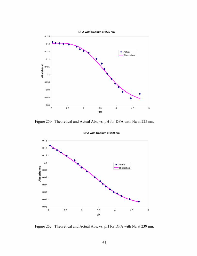
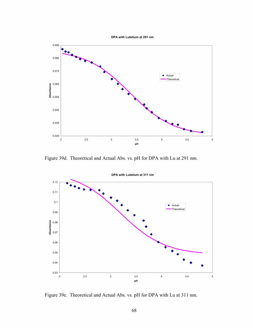
Lutetium. In Figures 39a-f, the graphs of our experimental and theoretical absorbances

plotted against pH are shown for DPA with lutetium at various wavelengths. The

experimental absorbance was recorded at 213 nm, 225 nm, 239 nm, 291 nm, 311 nm, and

319 nm. The Excel best-fit curve given by the global fit yielded at coefficient of

determination of 0.9865, and a standard error value of 0.0041. The calculated formation

constant for lutetium with DPA was 6.33 ± 0.02.

DPA with Lutetium at 213 nm

0.07

0.08

0.09

0.1

0.11

0.12

0.13

2 2.5 3 3.5 4 4.5

pH

Abs

orba

nce

5

ActualTheoretical

Figure 39a. Theoretical and Actual Abs. vs. pH for DPA with Lu at 213 nm.

66


0.055

0.065

0.075

0.085

0.095

0.105

0.115

0.125

0.135

2 2.5 3 3.5 4 4.5

pH

Abs

orba

nce

5

ActualTheoretical

Figure 39b. Theoretical and Actual Abs. vs. pH for DPA with Lu at 225 nm.


0.04

0.05

0.06

0.07

0.08

0.09

0.1

0.11

0.12

0.13

2 2.5 3 3.5 4 4.5

pH

Abs

orba

nce

5

ActualTheoretical

Figure 39c. Theoretical and Actual Abs. vs. pH for DPA with Lu at 239 nm.

67


0.025

0.035

0.045

0.055

0.065

0.075

0.085

0.095

2 2.5 3 3.5 4 4.5 5

pH

Abs

orba

nce

ActualTheoretical

Figure 39d. Theoretical and Actual Abs. vs. pH for DPA with Lu at 291 nm.


0.03

0.04

0.05

0.06

0.07

0.08

0.09

0.1

0.11

0.12

2 2.5 3 3.5 4 4.5 5

pH

Abs

orba

nce

ActualTheoretical

Figure 39e. Theoretical and Actual Abs. vs. pH for DPA with Lu at 311 nm.

68


0.02

0.04

0.06

0.08

0.1

0.12

0.14

0.16

2 2.5 3 3.5 4 4.5 5

pH

Abs

orba

nce

ActualTheoretical

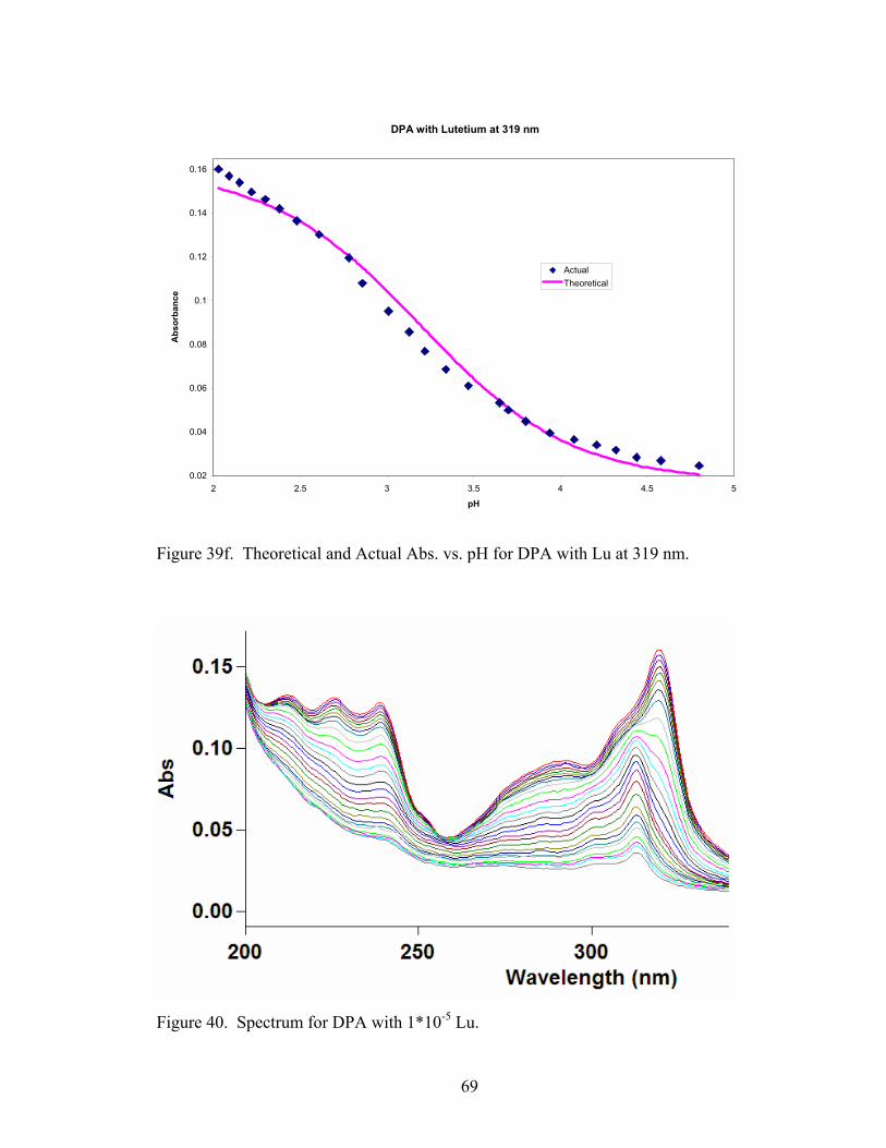
Figure 39f. Theoretical and Actual Abs. vs. pH for DPA with Lu at 319 nm.

Figure 40. Spectrum for DPA with 1*10-5 Lu.

69

Gadolinium. In Figures 41a-f, the graphs of our experimental and theoretical

absorbances plotted against pH are shown for DPA with gadolinium at various

wavelengths. The wavelengths at which experimental absorbances were recorded at are

213 nm, 225 nm, 239 nm, 291 nm, 311 nm, and 319 nm. The coefficient of

determination for the best-fit curve fitting the theoretical absorbances to the

corresponding dilution-adjusted experimental experimental absorbances in their

correlation with experimental pH was 0.9993. The standard error in the fitting of the

plots in Figures 41a-f was 0.0024. The resulting log K for DPA with gadolinium was

6.49 ± 0.06.

DPA with Gadolinium at 213 nm

0.25

0.255

0.26

0.265

0.27

0.275

0.28

0.285

0.29

0.295

0.3

0.305

2 2.5 3 3.5 4 4.5

pH

Abs

orba

nce

ActualTheoretical

Figure 41a. Theoretical and Actual Abs. vs. pH for DPA with Gd at 213 nm.

70


0.085

0.095

0.105

0.115

0.125

0.135

0.145

0.155

0.165

2 2.5 3 3.5 4 4.5

pH

Abs

orba

nce

ActualTheoretical

Figure 41b. Theoretical and Actual Abs. vs. pH for DPA with Gd at 239 nm.


0.03

0.04

0.05

0.06

0.07

0.08

0.09

0.1

0.11

2 2.5 3 3.5 4 4.5

pH

Abs

orba

nce

ActualTheoretical

Figure 41c. Theoretical and Actual Abs. vs. pH for DPA with Gd at 291 nm.

71


0

0.01

0.02

0.03

0.04

0.05

0.06

0.07

0.08

2 2.5 3 3.5 4 4.5

pH

Abs

orba

nce Actual

Theoretical

Figure 41d. Theoretical and Actual Abs. vs. pH for DPA with Gd.


0.01

0.02

0.03

0.04

0.05

0.06

0.07

0.08

0.09

0.1

2 2.5 3 3.5 4 4.5

pH

Abs

orba

nce

ActualTheoretical

Figure 41e. Theoretical and Actual Abs. vs. pH for DPA with Gd.

72


-0.01

0.01

0.03

0.05

0.07

0.09

0.11

0.13

0.15

2 2.5 3 3.5 4 4.5

pH

Abs

orba

nce

ActualTheoretical

Figure 41f. Theoretical and Actual Abs. vs. pH for DPA with Gd.

Figure 42. Spectrum for DPA with 1*10-5 Gd.

73

Strontium. In Figures 43a-f, the graphs of our experimental and theoretical absorbances

plotted against pH are shown for DPA with strontium at various wavelengths. The






resulting log K for DPA with strontium was 8.02 ± 0.08.

DPA with Strontium at 213 nm

0.08

0.085

0.09

0.095

0.1

0.105

0.11

0.115

0.12

2 2.5 3 3.5 4 4

pH

Abs

orba

nce

.5

actualtheoretical

Figure 43a. Theoretical and Actual Abs. vs. pH for DPA with Sr at 213 nm.

74


0.07

0.08

0.09

0.1

0.11

0.12

2 2.5 3 3.5 4 4

pH

Abs

orba

nce

.5

actualtheoretical

Figure 43b. Theoretical and Actual Abs. vs. pH for DPA with Sr at 225 nm.


0.055

0.065

0.075

0.085

0.095

0.105

0.115

2 2.5 3 3.5 4 4

pH

Abs

orba

nce

.5

actualtheoretical

Figure 43c. Theoretical and Actual Abs. vs. pH for DPA with Sr at 239 nm.

75


0.03

0.04

0.05

0.06

0.07

0.08

0.09

2 2.5 3 3.5 4 4.5

pH

Abs

orba

nce

actualtheoretical

Figure 43d. Theoretical and Actual Abs. vs. pH for DPA with Sr at 291 nm.


0.055

0.065

0.075

0.085

0.095

0.105

0.115

2 2.5 3 3.5 4

pH

Abs

orba

nce

4.5

actualtheoretical

Figure 43e. Theoretical and Actual Abs. vs. pH for DPA with Sr at 311 nm.

76


0.03

0.05

0.07

0.09

0.11

0.13

2 2.5 3 3.5 4 4

pH

Abs

orba

nce

.5

actualtheoretical

Figure 43f. Theoretical and Actual Abs. vs. pH for DPA with Sr at 319 nm.

Figure 44. Spectrum for DPA with 1*10-3 Sr.

77

3D Fluorescence

DPA proved difficult to study in aqueous solution for fluorescence stuides. As all

these studies were performed with DPA at the concentration of 1*10-8 M, the ionic

strength was roughly two orders of magnitude less than that of the stock DPA solution

and solutions used in the UV/Vis analyses. The drop in ionic strength on the scale of 2

orders of magnitude was an effect of diluting the DPA from a micromolar stock to a

sample concentration of 1x10-8 M, and diluting with ultra pure Milli-Q without correcting

the ionic strength for dilution. This is believed be the cause of the strong inconsistencies

between runs of the same concentration of DPA and/or metal. This is believed to be an

effect of pi-stacking. The strong non-polar character of the ligand DPA is believed to

have led to aggregation of the ligand molecules, which led to the inconsistent values

between results. As such, the following fluorescence data should be viewed as valuable

in a qualitative sense, but not quantitatively.

The following two spectra given as Figures 45a-b give a 3-dimensional view of

fluorescence intensity of free DPA at the concentration of 1x10-8 M as a function of

emission and excitation wavelengths(a), and a 2-dimensional view given in (b).

78

Figure 45a. 3D Fluorescence spectrum of DPA at pH 3.5.

79

Figure 45b. Fluorescence spectrum of DPA at pH 3.5.

In comparison to the spectrum at pH 3.5, when the pH of the sample solution is

raised to 5.0, the resulting spectrum can be seen in Figure 46, with a drop in magnitude of

fluorescence. This is partly due to the further deprotonation of the nitrogens of DPA,

which leads to the further quenching of fluorescence by the electron pairs of the DPA

nitrogens. Note the autoscaled plot read to a fluorescence of 5 for the free ligand at pH

3.5, but appeared at a maximum of 3.0 for the free ligand at pH 5.0.

80

Figure 46. Fluorescence spectrum of DPA at pH 5.0.

The fluorescence spectrum of a sample solution of 1*10-8 M DPA in 1*10-2 M

calcium yielded a maximum scaling for fluorescence in Q.S.E. of 8, as shown in Figure

47. This is clearly a shifted peak as compared to the free ligand at the same pH, which

indicates complexation of the metal ion calcium by DPA and shows in intensification in

fluorescence upon binding.

81

Figure 47. 3D Fluorescence spectrum of DPA with 1*10-2 M Ca at pH 3.5.

The spectra given in Figures 48a-b respresent both the 3-dimensional(a) and

2-dimensional(b) fluorescence spectra of a sample of 1*10-8 M DPA in 1*10-8 M

cadmium. Just as in the case of calcium with DPA, we see an increase in fluorescence as

compared to the free ligand at a pH of 3.5. In the case of cadmium, there is a noted jump

in fluorescence of roughly a factor of 10 upon the binding of cadmium by DPA as

compared to the free ligand at pH 3.5. The maximum scaling of fluorescence in Q.S.E.

in Figures 48a-b in the binding of cadmium is 50.

82

Figure 48a. 3D Fluorescence spectrum of DPA with 1*10-8 M Cd at pH 3.5.

83

Figure 48b. Fluorescence spectrum of DPA with 1*10-8 M Cd at pH 3.5.

The fluorescence spectra shown in Figures 49a-b are from a sample of 1:1

DPA:lead, both at 1*10-8 M. Lead, with its lone pair effect on DPA upon binding, was

expected to show a decrease in fluorescence as compared to the free ligand DPA at pH

3.5. The maximum fluorescence scaling for figures 49a-b is 2.0. There is a peak shift, as

well as a drop in fluorescence, as is expected upon the complexation of lead with DPA.

84

Figure 49a. 3D Fluorescence spectrum of DPA with 1*10-8 M Pb at pH 3.5.

85

Figure 49b. Fluorescence spectrum of DPA with 1*10-8 M Pb at pH 3.5.

The binding of mercury was expected to yield a drop in the fluorescence intensity

as lead did. The lone pair of electrons on mercury was expected to quench the

fluorescence of DPA upon binding as compared to the free DPA. The ligand behaved as

expected, and the spectrum of 1*10-8 M DPA in 1*10-8 mercury is given in Figures 50a-

b, with 50a showing the 3-dimensional spectrum, and 50b providing the 2-dimensional

view. The spectrum of the DPA-mercury complex showed a clear shift in peak structure

86

when compared to the free DPA at pH 3.5, and also showed an overall decrease in

fluorescence.

Figure 50a. 3D Fluorescence spectrum of DPA with 1*10-8 M Hg at pH 3.5.

87

Figure 50b. Fluorescence spectrum of DPA with 1*10-8 M Hg at pH 3.5.

The spectra in Figures 51a-b are the 3-dimensional(a) and 2-dimensional(b) views

of fluorescence spectra for a sample containing 1*10-8 M of both DPA and zinc.

Complexation of zinc decreased the fluorescence of DPA upon binding. Zinc cannot

fully span the cavity and complex all the available lone pairs of electrons donated by

DPA during complexation. This presence of a lone pair not involved in a bond with the

complexed zinc serves to decrease fluorescence. Behaving similarly to mercury and lead,

88

the complexation of zinc with DPA proves to decrease the fluorescence properties of free

DPA.

Figure 51a. 3D Fluorescence spectrum of DPA with 1*10-8 M Zn at pH 3.5.

89

Figure 51b. Fluorescence spectrum of DPA with 1*10-8 M Zn at pH 3.5.

The unprecedented binding of sodium to DPA with a given formation constant of

1.95 as found by the UV/Vis method is supported by the fluorescence scan given in

Figure 52. The spectrum below shows a strong increase in the fluorescence as well as a

peak shift from the spectrum of free DPA taken at pH 5.0, which is indicative that the

sodium is binding to the DPA.

90

Figure 52. 3D Fluorescence spectrum of DPA with 1*10-1 M Na at pH 5.0.

91

COMPUTATIONAL RESULTS AND DISCUSSION

DFT Calculations- Fluoride Affinity

For the theoretical reaction shown in Figure 53 of a hexaquo-metal ion reacting

with HF resulting ion the metal ion picking up a fluoride anion and losing a water, which

picks up a proton.

Figure 53. Theoretical reaction studied for fluoride affinity.

The Gibbs’ free energy of this theoretical reaction was calculated at 298 K for seven

metals: Co, Cr, Ga, Mn, Sc, In, and Y. The idea was to correlate the calculated

thermodynamic data in the gas phase to the known formation constants of the given

metals with fluoride in the aqueous phase. Formation constants for various metal ions

with the fluoride anion are shown in Table 9.

92

Table 9. Known formation constants for metals with fluoride.

In Figures 54 and 55, the decline of free energy is accompanied by an increase in the

formation constant of a given metal with fluoride. Increasingly negative changes in free

energy for the reaction laid out in Figure 53 would be expected to correlate to an

enhanced favorability in the binding of fluoride, and larger log K values. The plots show

exactly this.

93

Figure 54. 1st-row transition metal results of correlation of formation constants with ΔG.

Figure 55. Lanthanide results for correlation of experimental log K values with ΔG.

94

Data taken within the same row correlate well using this method, however,

comparing values of Gibbs free energy change for the theoretical reaction among

variations in mass that are too large results in very poor correlation.

95

Molecular Mechanics Calculations- Chelate Ring Size

The computational data from the isodesmic reaction investigating chelate ring size

theory is given in Table 10. Four metals of group 2A to give a representative ionic radius

range of 0.66 Å to 1.43 Å.

Steric E Ionic

Radius ΔE 5m 13.506988 Mg 29.178785 0.66 -4.871193 Ca 47.425159 0.99 -3.541393 Ba 61.911716 1.34 -1.615982 Ra 66.371864 1.43 -1.876934 6m 10.158195 Mg 20.958799 Ca 40.534973 Ba 56.946941 Ra 61.146137

Table 10. Chelate Ring Size Computational Data.

The data shows a coefficient of determination of 0.969, and a correlation

coefficient of 0.984. The trend is clearly linear in Figure 56, and shows a trend of

increasing steric energy for the isodesmic reaction as the ionic radius of the complexed

metal increases. The isodesmic scheme itself involved the transfer of a metal ion from a

five-membered chelate ring complex to a six-membered chelate ring complex.

According to chelate ring size theory, larger metal ions show a greater degree of

destabilization as the chelate ring size increases. This computational data shows that as a

clearly linear trend.

96

Steric Energy vs. Ionic Radius of Complexed Metal

y = 4.2601x - 7.6838R2 = 0.969

-5

-4.5

-4

-3.5

-3

-2.5

-2

-1.50.55 0.85 1.15 1.45

Ionic Radius

Ster

ic E

(kca

l/mol

Figure 56. Plot showing computational confirmation of chelate ring size theory.

97

Molecular Mechanics Calculations- Metal-N bond Length

For the following series of calculations, no “reactions” were performed, but rather

a comparison of different metals substituted into the same ligand, DPA. The series of 18

metals listed in Table 11 were substituted into the cavity of DPA with two waters

attached. After each substitution, MM+ geometry optimizations were run on each

structure and the minimum steric energy, labeled “Steric Ecalc” in Table 11, was recorded.

Table 11. MM+ computational data for ideal M-N bond length.

The “Avg. M-N b.l.” column of Table 11 represents the average of the three metal-

nitrogen bond lengths (M-N) found in each minimized structure. The calculated steric

energy was plotted against the average M-N bond length, and is shown in Figure 57.

98

Steric Energy (kcal/mol) vs. Average M-N Bond Length (Angstroms)

4

6

8

10

12

14

16

18

1.90 2.10 2.30 2.50 2.70

Average M-N Bond Length (Angstroms)

Ster

ic E

nerg

y (k

cal/m

ol)

ComputationalBest-Fit Calculated

Figure 57. Plot for determination of ideal metal-nitrogen bond length.

The data was fit to a combination Morse potential/2nd order polynomial using six

fitting parameters (A-F)) to fit the general equation

y = A(1-e-B(x-C))2 – (Dx2 + Ex + F).

The “Steric Etheor” column of Table 11 gives the values of the steric energy as calculated

by the equation fit to the energy minimization data. The “difference” column in Table 11

gives the squared difference between the “Steric Ecalc” and “Steric Etheor” columns, and

the square root was taken of the average of these values to provide the “Avg Diff” value

at the bottom of Table 11. This “Avg Diff” cell was minimized to a lower limit of zero,

using the fitting parameters A-F in order to attain the best fit the model would allow.

The derivative of the best fit equation was taken, and the zero of the equation was found

99

to be at the point where the average M-N bond length was equal to 2.38, with a

coefficient of determination of 0.9916.

100

Molecular Mechanics Calculations- Ideal Metal Ionic Radius

Just as in the determination of the ideal M-N bond length, this determination of

the ideal metal ionic radius will involve the comparison of metal-substituted DPA energy

minimized structures. The sixteen metal ions listed in Table 12 were substituted into

DPA with two waters attached to the bound metal ion. The structures were energy

minimized, and their minimum energies were recorded in the “Steric Ecalc” column of

Table 12. The known ionic radii of the metal ions were listed as well, for the purpose of

curve fitting and plotting later in the analysis.

Table 12. MM+ computational data for ideal ionic radius.

The calculated minimum steric energies and the corresponding ionic radii of the

bound metals of each structure were plotted in Figure 58. The resultant curve was locally

parabolic, so a 2nd order polynomial was once again fit to the data, just as in the

determination of the ideal M-N bond length, utilizing the same fitting means.

In this case, the ideal metal ionic radius was found at the minimum of the fitted curve to

be at 1.12 Å.

101

Determination of Ideal Metal Ionic Radius

y = 29.976x2 - 67.307x + 44.949R2 = 0.8394

0

5

10

15

20

25

0.5 0.6 0.7 0.8 0.9 1 1.1 1.2 1.3 1.4 1.5

Ionic Radius (Angstroms)

Ste

ric E

nerg

y (k

cal/m

ol)

Figure 58. Plot for determination of ideal metal ionic radius.

The Solver statistics add-in for Microsoft Excel was used to compute the error

statistics in fitting the curve to our computational data. The standard error associated in

curve fitting is 1.53, while the coefficient of determination is 0.8394. The scatter appears

randomly distributed to either side of the curve in Figure 58.

102

CONCLUSIONS

The rigid hemicycle DPA has a binding cavity containing three nitrogen donor

atoms, and two bound hydrogens within when fully protonated. The UV/Vis

spectrophotometric analysis showed two protonation events. As pH is raised, the first of

the two protons left with a pKa1 of 2.22 ± 0.03. The remaining proton left with a pKa2

of 4.52 ± 0.06.

Upon the binding of a metal, it was found that pKa1 remained constant at 2.22, as

the first proton had to leave before metal complexation could occur. After the first proton

was lost, there was only one other event present in all metal titrations analyzed, and that

occurred at the same time as the loss of the second proton from the binding cavity. At the

time of the loss of the final proton from the cavity, the metal would complex with DPA.

While a series of ten metals were analyzed by UV/Vis spectrophotometric

titration, a few stand out from the rest. As DPA has a pair of 5-membered chelate rings

formed in the complexation of a metal by its three nitrogen donors, it is expected to bind

large metal ions. The highest two formation constants found for the complexation of a

metal by DPA were with mercury and strontium, with formation constants of 8.16 ± 0.06

and 8.02 ± 0.01, respectively. The ionic radii of mercury and strontium are 1.10 and 1.12

Å, respectively. The best-fit ionic radius for a metal complexing to DPA, as determined

by the molecular mechanics calculations run in this research was 1.12 Å. This

computational work strongly backs up the results yielding the formation constants being

associated with metals with ionic radii very close to the calculated ideal.

While it appears to be the weakest formation constant measured, sodium

complexed surprisingly strongly with DPA. The ligand EDTA is known to bind sodium

103

with a log K of 1.85, while DPA binds sodium at a log K of 1.95 ± 0.04. While EDTA is

a hexadentate ligand, meaning it has six points of attachment and six donor atoms, our

ligand DPA is tridentate, with three donor atoms and three points of attachment. Further

comparing the two, DPA contains only nitrogen donors, which prefer intermediate metal

ions as defined by HSAB theory. EDTA contains four negatively charged oxygen

donors, which would prefer harder metal ions such as sodium. This would point to

EDTA having a larger formation constant with sodium than DPA, but this is not what is

observed. It is believed that it is the very high degree of preorganization and unique

nature of the binding cleft of this hemicycle that contributes to the unexpectedly high

binding constant with sodium. The ionic radius of sodium is 0.97, which is not an “exact

fit” for the binding cleft of DPA, it is certainly a reasonable fit, being close to within a

tenth of an Angstrom to the ideal ionic radius.

Let it also be noted that all of the Lanthanide metal ions that were analyzed via

UV/Vis spectrophotometry resulted in very similar formation constants with DPA. The

metal ions lanthanum, lutetium, and gadolinium have respective ionic radii of 1.06, 0.85,

and 0.94 Å. The formation constants of lanthanum, lutetium, and gadolinium are 6.43 ±

0.04, 6.33 ± 0.02, and 6.49 ± 0.06. Lanthanum and gadolinium based upon size alone

would be expected to show the largest formation constants of the three lanthanides

analyzed, and this was proven experimentally. Lanthanum and gadolinium also show

similar values for formation constants when the standard deviation is taken into account.

Lutetium is sufficiently smaller compared to the other two lanthanides analyzed that it

does not fit as well into the binding cleft of DPA, and this partly goes to explain its lower

value for the formation constant with DPA.

104

The analysis of the formation constants of these metals with DPA was only made

possible with the development and use of the dissolution method for large hemicycles

such as DPA. After many attempts, a simple four step method was chosen. In step one, a

sub-milligram amount of the ligand is weighed into a beaker using a sufficiently accurate

balance, such as a Cahn-microgram balance. Step two involves adding directly to the

ligand the concentrated acid necessary to bring the overall solution to the desired pH. In

step three, boiling Milli-Q water is added in small amounts over a period of a few hours

to bring the solution up to volume. The final step involves roto-vapping the solution

from step three to remove any solvents such as acetone that may have contaminated the

solution during the weighing process.

While formation constants are useful information, the end goal of studying this

ligand was to develop it for a practical use, such as a sensor. The fluorescence studies

completed for DPA proved to be quite useful qualitatively, but not quantitatively.

General trends of the existence or lack of fluorescence enhancement upon addition of a

metal was apparent, but any attempt to make a calibration line proved to be futile. It is

believed that part of the problem in lack reproducability was in the composition of the

solutions, and the enhanced pi-stacking and aggregation into nanoparticles that this led to.

The samples studied by fluorescence were prepared with ionic strengths at least two

orders of magnitudes less than that of the stock solution and UV/Vis samples. This is

believed to contribute to the formation of aggregate nanoparticles of DPA molecules.

Further studies in fluorescence of DPA will involve studies completed in an ionic

strength closer to that of the stock solution, which will require running blanks reflecting

the true background medium rather than that of pure water.

105

DPA did behave exactly as expected when it comes to fluorescence with metal

ions. It fluoresced with calcium, cadmium, and also sodium. The fluorescence of the

sodium-DPA complex further indicated that the unexpected result of a log K of DPA with

sodium of 1.95 was indeed occurring. The fluorescence of DPA proved not only to not

increase, but to decrease slightly in the presence of zinc, lead, and mercury. The issues of

studying fluorescence properties in aqueous solution with DPA suspended in water would

not be expected to follow through to a sensor application, where the ligand would be

harnessed to a surface. So DPA still would have a future as a possible sensor agent for

metal ions such as calcium, cadmium, and sodium.

Ligand binding was further investigated with respect to its relationship to

thermodynamics through a series of density functional theory calculations. Good results

were obtained when thermodynamic data was compared within approximately the same

row of the periodic table. The change in gibbs free energy for a theoretical reaction

emulating the binding of a fluoride anion to a metal ion in exhange for a first shell water

molecule showed a decreasing trend as the experimental log K for fluoride for a

particular metal ion increased.

Chelate ring size was investigated through an isodesmic reaction using molecular

mechanics. The goal of finding a linear relationship between the steric energy of our

reaction and the ionic radii of complexed metal ions was successful, with a coefficient of

determination of 0.969, and a correlation coefficient of 0.984. The isodesmic reaction

involved the transfer of a metal ion from a five-membered chelate ring to a six-membered

chelate ring, and the calculations showed the reaction energy to become more positive

overall as metal ion size increased. This follows the general idea of chelate ring size

106

theory, because larger metal ions experience larger degrees of destabilization as chelate

ring size increases.

Continuing with molecular mechanics, the ideal metal ionic radius to bind to DPA

was found by the molecular mechanics MM+ calculations to be 1.12 Å, which agrees

with UV/Vis spectrophotometric results. Within the same calculation series, the ideal

average bond length between the three donor nitrogens on DPA with the complexed

metal was calculated to be 2.38 with a coefficient of determination in fitting the data of

0.9916. As the hemicycle DPA has a pair of five-membered chelate rings formed

between its three nitrogen donors and the complexed metal, it is expected from chelate

ring size theory to preferentially bind larger metal ions. Geometrically speaking, the

ideal bond length for a five-membered chelate ring would lie close to 2.5 Å, while the

ideal bond length for a six-membered ring would lie closer to 1.6 Å. The calculated bond

length is within 0.12 Å of the ideal bond length for a five-membered chelate ring donor.

While DPA proved to be difficult to study initially due to its high degree of

insolubility in aqueous solution, it proved well worth the trouble. The dissolution method

developed to study it has opened up a venue to study other ligands within its class which

were previously untouchable by our methods. It has proven to strongly bind a variety of

large metals, with strontium and mercury being the most tightly bound of the series.

With its fluorescence capability, with further study it shows promise to be a possible

sensor for metals such as cadmium, sodium, and calcium.

107

LITERATURE CITED

1. Guo Orvig, C.; Abrams, M. Chem. Rev. 1999, 99, 2201. 2. Messerschmidt, A.; Cygler, M.; Bode, W. (Eds.) Handbook of Metalloproteins; Wiley:

Hoboken, NJ, Vol. 3, 2004, pp. 443-756. 3. Dudev, T.; Lim., C. Chem. Rev. 2000, 103, 773.

4. http://w3.uniroma1.it/MEDICFISIO/FURA2.HTM 5. http://www.biotium.com/prodindex/Ca/fura2/fura2.htm 6. http://www.americanheart.org/presenter.jhtml?identifier=4493 7. Florin et al. The Need for Vigilance: The persistence of Lead Poisoning in Children.

Pediatrics 2005; 115. 1767-1768.

8. Seely, Dugal et al. EDTA Chelation Therapy for Cardiovascular Disease: A Systematic Review. BMC Cardiovascular Disorders 2005. vol 5, p 32.

9. Hancock, R. D., Martell, A. E., Chem. Rev., 1989, 89, 1875. 10. Hancock, R.D.; Martell, A. E., Metal Complexes in Aqueous Solutions; Plenum: NY,

NY, 1996. 11. Pearson, Ralph. Hard and Soft Acids and Bases. J. ACS. Vol. 85 No. 22 (1963). 12. Yang, A.H., MacGillivray, R.T., Chen, J., Luo, Y., Wang, Y., Brayer,

G.D., Mason, A.B., Woodworth, R.C., Murphy, M.E. Crystal structures of two mutants (K206Q, H207E) of the N-lobe of human transferrin with increased affinity for iron. Protein Sci. 2000, 9, pp.49-52 .

13. Cram, D.J. Science 240 (1988) 76. 14. Cram et al. Chem. Commun., 1997, 1303-1304. 15. Alberto et al. J. Am. Chem. Soc., 2001, 3135-3136. 16. Hancock, R.D., McDougall, G. Origin of macrocyclic enthalpy. J. Am. Chem. Soc.;

1980; 102(21); 6551-6553. 17. Skoog, Holler, and Nieman. Principles of Instrumental Analysis; Thompson:

Singapore, 1998.

108

Documents

METAL ION COMPLEXING AND FLUORESCENCE ... Calculations – Fluoride Affinity 32 Molecular Mechanics Calculations-Chelate Ring Size 33 Molecular Mechanics Calculations-Ideal Ionic Radius