Embed Size (px)
Citation preview

HAL Id: hal-00091746https://hal.archives-ouvertes.fr/hal-00091746
Submitted on 20 May 2013
HAL is a multi-disciplinary open accessarchive for the deposit and dissemination of sci-entific research documents, whether they are pub-lished or not. The documents may come fromteaching and research institutions in France orabroad, or from public or private research centers.
L’archive ouverte pluridisciplinaire HAL, estdestinée au dépôt et à la diffusion de documentsscientifiques de niveau recherche, publiés ou non,émanant des établissements d’enseignement et derecherche français ou étrangers, des laboratoirespublics ou privés.
Inpainting and zooming using sparse representationsJalal M. Fadili, Jean-Luc Starck, Fionn Murtagh
To cite this version:Jalal M. Fadili, Jean-Luc Starck, Fionn Murtagh. Inpainting and zooming using sparse rep-resentations. The Computer Journal, Oxford University Press (UK), 2007, 52 (1), pp.64-79.<10.1093/comjnl/bxm055>. <hal-00091746>
Inpainting and Zooming Using
Sparse Representations
M.J. FADILI1, J.-L. STARCK2 AND F. MURTAGH3,*
1GREYC CNRS UMR 6072, Image Processing Group, ENSICAEN 14050, Caen Cedex, France2CEA-Saclay, DAPNIA/SEDI-SAP, Service d’Astrophysique, F-91191 Gif sur Yvette, France
3Department of Computer Science, Royal Holloway, University of London, Egham TW20 0EX, UK
*Corresponding author: [email protected]
Representing the image to be inpainted in an appropriate sparse representation dictionary, and
combining elements from Bayesian statistics and modern harmonic analysis, we introduce an expec-
tation maximization (EM) algorithm for image inpainting and interpolation. From a statistical
point of view, the inpainting/interpolation can be viewed as an estimation problem with missing
data. Toward this goal, we propose the idea of using the EM mechanism in a Bayesian framework,
where a sparsity promoting prior penalty is imposed on the reconstructed coefficients. The EM frame-
work gives a principled way to establish formally the idea that missing samples can be recovered/
interpolated based on sparse representations. We first introduce an easy and efficient sparse-
representation-based iterative algorithm for image inpainting. Additionally, we derive its theoreti-
cal convergence properties. Compared to its competitors, this algorithm allows a high degree of
flexibility to recover different structural components in the image (piecewise smooth, curvilinear,
texture, etc.). We also suggest some guidelines to automatically tune the regularization parameter.
Keywords: EM algorithm; sparse representations; inpainting; interpolation; penalized likelihood
Received 30 June 2006; revised 15 February 2007
1. INTRODUCTION
Inpainting is to restore missing image information based upon
the still available (observed) cues from destroyed, occluded or
deliberately masked subregions of the images. The keys to
successful inpainting are to infer robustly the lost information
from the observed cues. The inpainting can also be viewed as
an interpolation or a disocclusion problem. The classical
image inpainting problem can be stated as follows. Suppose
the ideal complete image is x defined on a finite domain V
(the plane), and its degraded version (but not completely
observed) y. The observed (incomplete) image yobs is the
result of applying the lossy operatorM on y
M : y 7! yobs ¼M½y� ¼ M½x� 1� ð1Þ
where � is any composition of two arguments (e.g. ‘þ’ for
additive noise, etc.), 1 is the noise. M is defined on VnE,
where E is a Borel measurable set. A typical example of Mthat will be used throughout this paper is the binary mask; a
diagonal matrix with ones (observed pixel) or zeros (missing
pixel), and yobs is a masked image with zeros wherever
a pixel is missing. Inpainting is to recover x from yobs,
which is an inverse ill-posed problem.
1.1. State of affairs
Non-texture image inpainting has received considerable inter-
est and excitement since the pioneering paper by Masnou and
Morel [1, 2] who proposed variational principles for image
disocclusion (the term inpainting was not used yet). A recent
wave of interest in inpainting has also started from the paper
of [3], where applications in the movie industry, video and
art restoration were unified. These authors proposed nonlinear
partial differential equations (PDE) for non-texture inpainting.
Basically, the major mechanisms to get information into the
inpainting domain are:
(i) Diffusion and transport PDE/Variational principle: in
[3–6], the PDE is obtained phenomenologically, and
axiomatically in [7]. Ballester et al. in a series of
papers [8–10], proposed to solve the inpainting
problem by considering a joint interpolation of the
orthogonal direction of level lines and of the gray
levels. In [11], the authors proposed a curvature-driven
THE COMPUTER JOURNAL, 2007
# The Author 2007. Published by Oxford University Press on behalf of The British Computer Society. All rights reserved.For Permissions, please email: [email protected]
doi:10.1093/comjnl/bxm055
The Computer Journal Advance Access published July 29, 2007
diffusion image inpainting method. Chan and Shen
[12] systematically investigated inpainting based on
the Bayesian and (possibly hybrid) variational prin-
ciples with different penalizations (TV, ‘1 norm on
wavelet coefficients). By functionalizing Euler’s elas-
tica energy, Masnou and Morel [1, 2], proposed an
elastica-based variational inpainting model, and [13]
developed its mathematical foundation and a PDE
computational scheme. Following in the footsteps of
Chan and Shen, authors in [1] adapted the
Mumford–Shah image segmentation model to the
inpainting problem. Chan et al. [15] also employed a
TV variational approach for joint image inpainting
and deblurring. They have recently applied this work
to superresolution [15].
There are other recent references concerned with
PDE/variational inpainting and the interested reader
may refer for example to the UCLA CAM reports
website1 for an abundant literature (e.g. [17, 18], etc.).
For an extended survey of the mathematics involved
in the above frameworks and some applications, see
[19, Chapter 6, 20]. Note however that the main intrin-
sic limitations of these approaches is that they cannot
deal with texture inpainting. They are suitable for geo-
metrical parts of the image and perform well only for
non-texture inpainting. Thus, texture and large empty
gaps can be a major issue.
(ii) Exemplar region fill-in: the basic idea behind these
algorithms is to fill-in the missing regions with avail-
able information from some best matching candidates
(e.g. surrounding pixels/regions [21, 22], best corres-
pondence maps [23]). The goal is to synthesize a com-
plete, visually plausible and coherent image, where the
visible parts of the image serve as a reference/training
set to infer the unknown parts. For example, in [21],
the authors proposed a Markov random field-based
synthesis approach only suitable for texture inpainting.
Bertalmıo and co-workers [22, 24] adapted Meyer’s
u þ v model to decompose the image into its natural
(cartoon) and texture parts, then inpaint the natural
part using a PDE-based method and a fill-in-based
approach for the texture part following the work of
[21]. Finally, the inpainted parts are recombined.
Other authors have also proposed to first restore the
geometrical (or natural) part combined with a fill-in
texture synthesis method [25, 26]. In work by Criminisi
et al. [27], the authors proposed an algorithm that
allows one to fill-in an image progressively by
looking for best-matching prototypes in a dictionary
built from a set of patterns around the missing
subregions. Drori et al. [28] also proposed a fill-in
image completion method which bears similarities
with [27], although the fill-in step was differently
approached.
(iii) Compressed/ive Sensing: more recently, [29] intro-
duced a novel inpainting algorithm that is capable of
reconstructing both texture and cartoon image con-
tents. This algorithm is a direct extension of the Mor-
phological Component Analysis (MCA), designed for
the separation of an image into different semantic
components [30, 31]. The arguments supporting this
method were borrowed from the very exciting and
recent theory of Compressed/ive Sensing recently
developed by Donoho [32], Donoho and Tsaig [33]
and Candes et al. [34–36].
1.2. This paper
Combining elements from statistics and modern harmonic
analysis theories, we here introduce an EM algorithm [37,
38] for image inpainting/interpolation based on a penalized
maximum-likelihood formulated using linear sparse represen-
tations, i.e. x ¼ Fa, where the image x is supposed to be effi-
ciently represented by a few atoms in the dictionary.
Therefore, a sparsity promoting prior penalty is imposed on
the reconstructed coefficients. From a statistical point of
view, the inpainting can be viewed as an estimation problem
with incomplete or missing data, where the EM framework
is a very general tool in such situations. The EM algorithm for-
malizes the idea of replacing the missing data by estimated
ones from coefficients of the previous iteration, and then we
reestimate the new expansion coefficients from the complete
formed data, and iterate the process until convergence. We
here restrict ourselves to zero-mean additive white Gaussian
noise (AWGN), even if the theory of the EM can be developed
for the regular exponential family. The EM framework gives a
principled way to establish formally the idea that missing
samples can be recovered based on sparse representations.
Furthermore, owing to its well-known theoretical properties,
the EM algorithm allows us to investigate the convergence
behavior of the inpainting algorithm. Some results are
shown to illustrate our algorithm on inpainting, zooming and
disocclusion tasks.
This paper is organized as follows. In Section 2, we will
introduce the necessary ingredients of sparse representations
and concepts from modern harmonic analysis. In Section 3,
we state the inpainting problem, give the necessary material
about the EM mechanism and Bayesian estimation, and the
inpainting algorithm is also introduced. Section 4 states
some key convergence analysis results whose proofs are out-
lined in the Appendix, and discusses the influence of the regu-
larization parameter. Section 5 is devoted to presenting and
discussing experimental results including inpainting and
zooming. We conclude with a brief summary of our work
and some perspectives on its likely future development.1http://www.math.ucla.edu/applied/cam/index.html
Page 2 of 16 M.J. FADILI, J.-L. STARCK AND F. MURTAGH
THE COMPUTER JOURNAL, 2007
1.3. Notation
LetH a real Hilbert space, which is in our finite-dimensional case,
a subset of the vector space Rn. We denote by k.k2 the norm
associated with the scalar product inH, and I is the identity opera-
tor onH.The x andaare, respectively, reorderedvectorsof image
samples and transform coefficients. Let f:H 7! R < f1g, where
the domain of f is dom f ¼ fx [ H j f(x) , 1g. A function is
proper if its domain is non-empty, i.e. not identically þ1 every-
where. A function f is coercive, if limkxk2!þ1 f(x) ¼ þ1.
2. SPARSE IMAGE REPRESENTATION
2.1. Sparse representations
Suppose x [H. Anp
n �p
n image x can be written as the
superposition of (a few) elementary functions fg(s) (atoms)
parameterized by g [ G such that (G is countable)
xðsÞ ¼Xg[G
agfgðsÞ; CardG ¼ L: ð2Þ
Popular examples of G include: frequency (Fourier), scale-
translation (wavelets), scale-translation-frequency (wavelet
packets), translation-duration-frequency (cosine packets),
scale-translation-angle (e.g. curvelets, bandlets, contourlets,
wedgelets, etc.). The dictionary F is the n � L matrix whose
columns are the generating atoms ffggg[G, which are sup-
posed to be normalized to a unit ‘2-norm. The forward trans-
form is defined via a non-necessarily square full rank matrix
T ¼ FT [ RL�n, with L � N. When L . n the dictionary is
said to be redundant or overcomplete.
Owing to recent advances in modern harmonic analysis,
many redundant systems, like the undecimated wavelet trans-
form, curvelet, contourlet, steerable or complex wavelet pyra-
mids, were shown to be very effective in sparsely representing
images. By sparsity, we mean that we are seeking a good repre-
sentation of x with only very few non-zero coefficients, i.e.
kak0 � n. In most practical situations, the dictionary is
built by taking the union of one or several (sufficiently inco-
herent) transforms, generally each corresponding to an orthog-
onal basis or a tight frame. In the case of a simple orthogonal
basis, the inverse transform is trivially F ¼ TT; whereas
assuming that T is a tight frame implies that the frame operator
satisfies TTT ¼ cI, where c . 0 is the tight frame constant.
Hence, TT ¼ F is the Moore–Penrose pseudo-inverse trans-
form (corresponding to the minimal dual synthesis frame),
up to the constant c. In other words, the pseudo-inverse recon-
struction operator Tþ reduces to c21F.
2.2. Choosing a dictionary
Choosing an appropriate dictionary is a key step toward a good
sparse representation, hence inpainting and interpolation.
A core idea here is the concept of morphological diversity,
as initiated in [30]. When the transforms are amalgamated in
one dictionary, they have to be chosen such that each leads
to sparse representations over the parts of the images it is
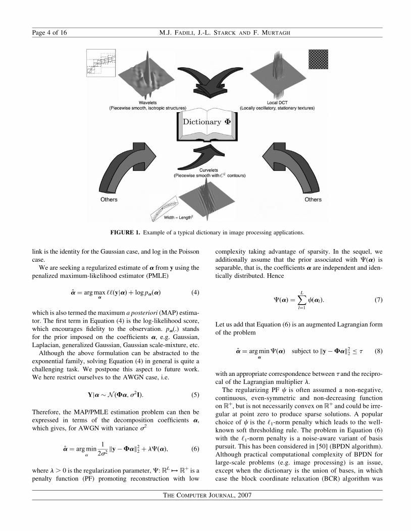
serving. Thus, for example (see Fig. 1), to represent efficiently
isotropic structures in an image, a qualifying choice is the
wavelet transform [39, 40]. The curvelet system [41, 42] is a
very good candidate for representing piecewise smooth (C2)
images away from C2 contours. The ridgelet transform [43,
44] has been shown to be very effective for representing
global lines in an image. The local discrete cosine transform
(DCT) [39] is well suited to represent locally stationary tex-
tures. These transforms are also computationally tractable par-
ticularly in large-scale applications, and never explicitly
implementing F and T. The associated implicit fast analysis
and synthesis operators have typically complexities of O(n)
(e.g. orthogonal or bi-orthogonal wavelet transform) or
O(n log n) (e.g. ridgelet, curvelet, local DCT transforms).
Another desirable requirement that the merged transforms
have to satisfy is that when a transform sparsely represents a
part in the image, it yields non-sparse representations on the
other content type. This is intimately related to the concept
of mutual incoherence, which plays a fundamental role in
sparse solutions of overcomplete (redundant) linear systems.
For a given dictionary, it is defined as the maximum in magni-
tude of the off-diagonal elements of its Gram matrix (see
e.g. [45–48] for more details).
3. PENALIZED MAXIMUM-LIKELIHOOD
ESTIMATOR WITH MISSING DATA
3.1. Penalized maximum-likelihood estimator
estimation
First, let’s ignore the missing data mechanism and consider the
complete n-dimensional observed vector (by simple reorder-
ing) y. Adopting a GLM framework, we assume that y has
a density in the classical exponential family, taking the
form [49]
fYðy;h;sÞ ¼ hðy;sÞ exphTy� AðhÞ
gðsÞ
� �ð3Þ
for some specific functions A(.), g(.) and h(.), h is the canonical
parameter and s is the scale parameter. From classical results
on exponential families [49], the mean of Y is related to hvia E[Yi] ¼ a0(hi), because typically, A(h) ¼
Pi¼1n a(hi).
There also exists a one-to-one transform, called the link func-
tion, relating E[Y] to Fa. The most important case corresponds
to the canonical link function (a0)21(.), or h ¼Fa, that is
(Fa)i ¼ (a0)21(E[Yi]). In this case, a can be viewed as par-
ameters of a canonical sub-family of the original exponential
family with sufficient statistic FTY. For instance, the canonical
INPAINTING AND ZOOMING USING SPARSE REPRESENTATIONS Page 3 of 16
THE COMPUTER JOURNAL, 2007
link is the identity for the Gaussian case, and log in the Poisson
case.
We are seeking a regularized estimate of a from y using the
penalized maximum-likelihood estimator (PMLE)
a ¼ arg maxa‘‘ðyjaÞ þ log paðaÞ ð4Þ
which is also termed the maximum a posteriori (MAP) estima-
tor. The first term in Equation (4) is the log-likelihood score,
which encourages fidelity to the observation. pa(.) stands
for the prior imposed on the coefficients a, e.g. Gaussian,
Laplacian, generalized Gaussian, Gaussian scale-mixture, etc.
Although the above formulation can be abstracted to the
exponential family, solving Equation (4) in general is quite a
challenging task. We postpone this aspect to future work.
We here restrict ourselves to the AWGN case, i.e.
Yja � NðFa;s2IÞ: ð5Þ
Therefore, the MAP/PMLE estimation problem can then be
expressed in terms of the decomposition coefficients a,
which gives, for AWGN with variance s2
a ¼ arg mina
1
2s2ky�Fak22 þ lCðaÞ; ð6Þ
where l . 0 is the regularization parameter, C: RL 7! Rþ is a
penalty function (PF) promoting reconstruction with low
complexity taking advantage of sparsity. In the sequel, we
additionally assume that the prior associated with C(a) is
separable, that is, the coefficients a are independent and iden-
tically distributed. Hence
CðaÞ ¼XL
l¼1
cðalÞ: ð7Þ
Let us add that Equation (6) is an augmented Lagrangian form
of the problem
a ¼ arg mina
CðaÞ subject to ky�Fak22 � t ð8Þ
with an appropriate correspondence between t and the recipro-
cal of the Lagrangian multiplier l.
The regularizing PF c is often assumed a non-negative,
continuous, even-symmetric and non-decreasing function
on Rþ, but is not necessarily convex on Rþ and could be irre-
gular at point zero to produce sparse solutions. A popular
choice of c is the ‘1-norm penalty which leads to the well-
known soft thresholding rule. The problem in Equation (6)
with the ‘1-norm penalty is a noise-aware variant of basis
pursuit. This has been considered in [50] (BPDN algorithm).
Although practical computational complexity of BPDN for
large-scale problems (e.g. image processing) is an issue,
except when the dictionary is the union of bases, in which
case the block coordinate relaxation (BCR) algorithm was
FIGURE 1. Example of a typical dictionary in image processing applications.
Page 4 of 16 M.J. FADILI, J.-L. STARCK AND F. MURTAGH
THE COMPUTER JOURNAL, 2007
proposed as a fast and effective algorithm [51]. Minimizers
of Equation (6) for a general class of regularizing func-
tions (neither non-necessarily differentiable nor convex)
have been characterized in a rigorous and systematic way
for the orthogonal wavelet transform in [52], and general
F in [53]. However, in the latter, implementation issues
were not considered except for the simple orthogonal case.
Inspired by the BCR, Elad [54] recently proposed a parallel
coordinate descent approach for iteratively solving Equation
(6) with overcomplete F and the ‘1-norm penalty. A conver-
gence analysis of this algorithm was recently proposed in
[55], but only with a smoothed and strictly convexified
version of the ‘1 penalty, which is an important and strong
assumption.
3.2. Derivation of E and M steps
Let us now turn to the missing data case and let us write y ¼
(yo, ymiss), where ymiss ¼ fyigi[Imis the missing data, and yo ¼
fyigi[Io. The incomplete observations do not contain all
information to apply standard methods to solve Equation
(6) and get the PMLE of u ¼ (aT, s2)T [ Q , RL� Rþ*.
Nevertheless, the EM algorithm can be applied to iteratively
reconstruct the missing data and then solve Equation (6) for
the new estimate. The estimates are iteratively refined until
convergence.
3.2.1. The E step
This step computes the conditional expectation of the pena-
lized log-likelihood of complete data, given yo and current
parameters u (t) ¼ (a (t)T
, s2(t)
)T
Q ujuðtÞ� �
¼ E ‘‘ðyjuÞ � lCðaÞjyo;uðtÞ
� �¼ E ‘‘ðyjuÞjyo; u
ðtÞ� �
� lCðaÞ: ð9Þ
For regular exponential families, the E step reduces to finding
the expected values of the sufficient statistics of the complete
data y given observed data yo and the estimate of a (t) and s2(t)
.
Then, as the noise is zero-mean white Gaussian, the E-step
reduces to calculating the conditional expected values and
the conditional expected squared values of the missing data,
that is
yðtÞi ¼ E yijF; yo;a
ðtÞ;s2ðtÞh i
¼yi; for observed data; i [ Io;
ðFaðtÞÞi for missing data; i [ Im;
(
and Ehy2
i jF; yo;aðtÞ;s2ðtÞ
i¼
y2i ; i [ Io;
ðFaðtÞÞ2i þ s2ðtÞ ; i [ Im:
(
ð10Þ
3.2.2. The M step
This step consists of maximizing the penalized surrogate func-
tion with the missing observations replaced by their estimates
in the E step at iteration t, that is
uðtþ1Þ ¼ arg minu[Q
�Q ujuðtÞ� �
: ð11Þ
Thus, the M step updates s2(tþ1)
according to
s2ðtþ1Þ
¼1
n
Xi[Io
yi � FaðtÞ� �
i
� �2þðn� noÞs
2ðtÞ
" #; ð12Þ
where no ¼ trM ¼ CardIo is the number of observed pixels.
Note that at convergence, we will have
s2�!1
no
Xi[Io
ðyi � ðFaÞiÞ2
which is the maximum-likelihood estimate of the noise vari-
ance inside the mask (i.e. with observed pixels).
As far as the update equation of a (tþ1) is concerned, this
depends not only on the structure of the dictionary F (i.e.
basis, tight frame, etc.), but also on the properties of the PF
c (i.e. smooth/non-smooth, convex/non-convex). These two
parameters also have a clear impact on the convergence beha-
vior of the inpainting algorithm. Important cases will be
treated separately in Section 4. In all cases, the overall struc-
ture of the EM-based inpainting algorithm is as follows.
Algorithm 1
Require: Observed image yobs ¼My and a maskM, t ¼ 0, initial
a (0)
1: repeat
2: E Step
3: Update the image estimate:
yðtÞ ¼ yobs þ ðI�MÞFaðtÞ ¼ FaðtÞ þ ðyobs �MFaðtÞÞ ð13Þ4: M Step
5: Solve Equation 6 with reconstructed y (t) substituted for y, and
get a (tþ1).
6: If desired, update s2(tþ1)
according to Equation 12.
7: t ¼ t þ 1,
8: until Convergence.
9: Reconstruct x from a.
If s2 happens to be known, step 6 can be dropped from the
updating scheme.
4. CONVERGENCE PROPERTIES
In this section, we shall give both the updating rules of a (tþ1)
and the convergence properties of the corresponding EM
INPAINTING AND ZOOMING USING SPARSE REPRESENTATIONS Page 5 of 16
THE COMPUTER JOURNAL, 2007
algorithm (and its variants) for different penalties and types of
dictionaries (the columns of which are always supposed to be
normalized to a unit ‘2-norm). Convergence is examined in
both the weak and strong topologies.
The convergence properties of the EM algorithm and its
generalizations [e.g. GEM, expectation conditional maximiza-
tion (ECM), see [38, 56]] have deeply been investigated by
many authors (see, e.g. [37, 38, 57]). However, most of their
results heavily rely on the smoothness of the log-likelihood
function or its penalized form, hence on the regularity of the
penalty c (e.g. Q(.j.) is C1 for many results to hold [57]).
But, to produce sparse solutions, we are mainly concerned
with non-smooth penalties. Thus, most of classical conver-
gence results of the EM and its variants do not hold here.
We therefore need more involved arguments that we mainly
borrow from non-smooth convex analysis and the optimi-
zation literature.
4.1. F is a basis
In this case, F is a bijective bounded linear operator. Algor-
ithm 1 is an EM, which can be solved for the coefficients a,
or equivalently, in terms of the image samples x.
Many sparsity promoting PFs have been proposed in the
literature. Although they differ in convexity, boundedness,
smoothness and differentiability, they generally share some
common features that we state here as general conditions for
a family of PFs considered in our setting. Suppose that:
H1. c is even-symmetric, non-negative and non-decreasing
on [0, þ1), and c(0) ¼ 0.
H2. c is twice differentiable on R\f0g, but not necessarily
convex.
H3. c is continuous on R, it is not necessarily smooth at
zero and admits a positive right derivative at zero
c0þð0Þ ¼ limh!0þ ðcðhÞ=hÞ . 0.
H4. The function a þ lc 0(a) is unimodal on (0, þ1).
Among the most popular PFs satisfying the above require-
ments, we cite c(a) ¼ jajp, 0 , p � 2 (generalized Gaussian
prior), c(a) ¼p
(a2þ n), n � 0, the SCAD penalties [52];
see, e.g. [52, 58] for a review of others.
PROPOSITION 1. If c respects H1–H4,
(i) The step has exactly one solution decoupled in each
coordinate zl ¼ fTl y (t):
alðzlÞ ¼0; ifjzlj � ls2c0þð0Þ;zl � ls2c0ðalÞ; ifjzlj . ls2c0þð0Þ;
�ð14Þ
which is continuous in zl.
(ii) The sequence of observed penalized likelihoods con-
verges (actually increases) monotonically to a statio-
nary point of the penalized likelihood.
(iii) All limit points of the EM inpainting sequence fx (t),
t �0g generated by Algorithm 1 are stationary points
of the penalized likelihood.
See Appendix for the proof.
PROPOSITION 2. If c satisfies H1–H4, is coercive and proper
convex.
(i) The inpainting problem has at least one solution.
(ii) The inpainting problem has exactly one solution if c is
strictly convex.
(iii) The instance of iterates fx (t), t � 0g is asymptotically
regular, i.e. kx (tþ1) 2 x (t)k ! 0, and converges
weakly to a fixed point.
(iv) If c(a) ¼ jajp, 1 � p � 2, the sequence of iterates con-
verges strongly to a solution of the inpainting problem.
See Appendix for the proof.
REMARK 1.
(i) When c(a) ¼ jaj, the shrinkage operator is the popular
soft thresholding rule. The EM inpainting with a basis
is then an iterative soft thresholding, which is strongly
convergent. Strong convergence can also happen with
other penalties thanc(a) ¼ jajp, p [ [1, 2]. For instance,
any strongly convex functioncwill imply strong conver-
gence (see [59, Corollary 5.16 and Proposition 3.6]).
(ii) The sequence of inpainting iterates is asymptotically
regular. This furnishes a simple stopping rule test, typi-
cally kx (tþ1)2 x (t)k ,d for sufficiently small d . 0.
(iii) If one has additional constraints to be imposed on the
solution such as forcing the image to lie in some closed
convex subset ofH (e.g. positive cone), the iteration in
Equation (A.2) can be easily adapted by incorporating
the projector onto the constraint set, e.g. replace DF,l
by Pþ 8 DF,l, (Pþx)i ¼ max(xi, 0).
4.2. F is a frame
F is no longer a bijective linear operator (surjective but not
injective). Consequently, the EM step will be solved in
terms of the transform coefficients. The inpainted image is
reconstructed after convergence of the EM algorithm. This
is a major distinction with the previous case of a basis.
Indeed, when solving the problem in terms of image (or
signal) samples, the solution x is allowed to be an arbitrary
vector over Rn, whereas the solution image is confined to
the column space of F when solving in terms of coefficients
a. This distinction holds true except when F is orthogonal.
We therefore propose the following proximal Landweber-like
iterative scheme, which summarizes the E and M steps
aðtþ1Þ ¼ Smls2 aðtÞ þ mFT yobs �MFaðtÞ� �� �
; m . 0;
ð15Þ
Page 6 of 16 M.J. FADILI, J.-L. STARCK AND F. MURTAGH
THE COMPUTER JOURNAL, 2007
where Smls2 is the componentwise shrinkage operator associ-
ated with Equation (14) with parameter mls2. Again,
the questions we want to answer are, for a general frame,
(i) does this algorithm converge, (ii) what is the convergence
behavior of such an iterative scheme, (iii) can the iteration
be computed efficiently? The answer to the first question is
yes under assumptions similar to the ones stated for the
basis case. This will be summarized shortly in a general
result together with an answer to question (ii). As far as
point (iii) is concerned, a positive answer cannot be given in
general since multiplications by F and FT are involved.
A very interesting case happens when the dictionary is a
tight frame. In such a case, following the discussion in
Section 2 (see also Remark 2), multiplications by F and T
are never explicitly implemented (fast implicit analysis and
synthesis operators are used instead).
We are now ready to state a convergence result for frames
PROPOSITION 3. Suppose that c satisfies H1–H4, is coercive
and proper convex. Moreover, suppose that 0 , m , 2/B,
where B is the frame upper bound. Then the following holds:
(i) The inpainting problem has at least one solution.
(ii) The inpainting problem has exactly one solution if c is
strictly convex.
(iii) The instance of coefficient iterates fa(t), t � 0g is
asymptotically regular and converges weakly to a
solution of the inpainting algorithm.
(iv) If c(a) ¼ jajp, 1 � p � 2, the sequence of coefficient
iterates converges strongly to a solution of the inpaint-
ing problem.
See Appendix for the proof.
REMARK 2.
(i) Again, for c(a) ¼ jaj, the EM inpainting with a frame
is a strongly convergent iterative soft thresholding.
Note also that the strong convexity of c is sufficient
for assertion (iv) in Proposition 3 to remain true.
(ii) Note that with frames, it becomes less straightforward
to impose some side constraints on the solution such as
positivity, compared to the previous case of bases.
(iii) An interesting special case of Equation (15) arises
when F is a tight frame (A ¼ B, Tþ ¼ B21F),
m ¼ B21 (2), and c (a) ¼ jaj. Letting k(t) ¼ Tyobs/B
þ (I 2 TMTþ)a(t), and specializing Equation (14)
to soft thresholding, Equation (15) becomes
aðtþ1Þl ¼
0; ifjkðtÞl j � ls2=B;
kðtÞl � signðkðtÞl Þls2=B; if jkðtÞl j . ls2=B:
(
ð16Þ
Except for the scaling by B, it turns out that this itera-
tion is a simple shrinkage applied to the data recon-
structed at the E step. It embodies an (implicit)
reconstruction step followed by an analysis and a
shrinkage step, and is very efficient to compute.
A similar iteration can be developed for any other
rule corresponding to any other appropriate penalty.
4.3. F is a union of transforms
Let us now assume the general case where the dictionary is a
union of K sufficiently incoherent transforms, that is F ¼ [F1,
. . . , FK]. In this case, the M step of the inpainting becomes
more complicated and computationally unattractive.
However, this maximization becomes much simpler when
carried out with respect to each transform coefficient with
the other coefficients held constant. In the statistical literature,
this generalized version of the EM is termed ECM [56, 60, 61].
Without the E step, this algorithm is also known as (block)
coordinate relaxation in optimization theory [62, 63].
More precisely, ECM replaces each M step of the EM, by a
cyclic sequence of K conditional optimization steps, each of
which minimizes the surrogate functional Q over ak, k [ f1,
. . . , Kg, with the other transform coefficients ak0=k fixed at
their previous value. The M step in Algorithm 1 then
becomes (we omit the update of s for briefness),
Compute the residual r (t) ¼ yobs 2MP
k¼1K Fkak
(t),
for Each transform k[ f1, . . . ,Kg in the dictionary do
CM Step: Solve the optimization problem
aðtþ1Þk ¼ arg min
ak
1
2s2
��� rðtÞ þFkaðtÞk
� ��Fkak
���2
2
þ lkCðakÞ ð17Þ
end for
The optimization subproblem for each k can be solved by
adapting results of the previous two sections depending on
whether Fk is a basis or a tight frame. Let us also mention
that a variation of the above ECM, termed multi-cycle ECM
in [56], would be to include an E step before each CM step,
which is equivalent to putting the E and CM steps inside the
loop over transforms.
Under appropriate regularity conditions on the complete
data penalized likelihood, it has been shown that the ECM
extension (which is actually a Generalized EM; see [37])
shares all the appealing convergence properties of the GEM
such as monotonically increasing the likelihood, convergence
(in the weak topology) to a stationary point, local or global
minimum, etc. (see [56, 57] for more details). However, for
many of their results to apply, smoothness and strict convexity
of the PF are again important assumptions (PF must be C1),2See the proof of Proposition 3 for the definition of A and B.
INPAINTING AND ZOOMING USING SPARSE REPRESENTATIONS Page 7 of 16
THE COMPUTER JOURNAL, 2007

which is not the case for the sparsity-promoting penalties
adopted here.
One strategy to circumvent this difficulty is to smooth at
zero the family of PFs we consider. Typically, many PFs ful-
filling requirements H1–H4 may be recast as functions of jaj.
Then, one may operate the change of variable in c(jaj) to
c(p
(a2þ n)) with sufficiently small n . 0. For example, the
PF corresponding to the ‘p-norm may be replaced with
(a2þ n)p/2, or with the function proposed in [55]. The latter
approximation has the advantage of providing a closed-form,
but approximate solution to Equation (14). Note also that
these approximations are strict convexification of the original
‘p PF. Hence, with the latter smooth and strictly convex PF
approximations, by straightforward adaptation of the results
in [56, 57], it can easily be shown that the penalized likelihood
converges monotonically to a stationary point, and that the
sequence of multi-cycle ECM iterates converges (weakly) to
the unique stationary point which is also the global maximizer
of the penalized likelihood.
The other strategy is to extend convergence results of the
ECM to non-smooth PFs. As in the previous sections, this
will be accomplished by exploiting the separable structure of
PF and appealing to more elaborated tools in optimization
theory, namely (block) coordinate relaxation-based minimi-
zation methods for non-differentiable functions [63, 64].
Note that the BCR algorithm has already been used for
‘1- regularized sparse denoising problems with overcomplete
dictionaries, but only for dictionaries which are a union of
bases, while our algorithm stated below will be valid even
for more complicated dictionaries and PFs.
4.3.1. General algorithm and its properties
Here is now our general multi-cycle ECM inpainting algori-
thm for dictionaries that are a union of several (incoherent)
transforms:
Algorithm 2
Require: Observed image yobs and a maskM, t ¼ 0, initial a(0),
8k [ f1, . . . , Kg, 0 , mk , 2/Bk,
1: repeat
2: Select a transform k [ f1, . . . , Kg with a cyclic rule.
3: r (t) ¼ yobs 2MP
k¼1K Fkak
(t),
4: for m ¼ 1 to M do
5: Update,
aðtþm=MÞk ¼ Smklks2 a
ðtþðm�1Þ=MÞk þ mkF
Tk
hrðtÞ þMFka
ðtÞk
� ��
�MFkaðtþðm�1Þ=MÞk Þ� ð18Þ
6: end for
7: t ¼ t þ 1,
8: until Convergence.
9: Reconstruct x from a.
Note that for a single transform, this algorithm reduces to
Equations (A.2) and (15) for respective corresponding cases.
The following result establishes the convergence behavior
of the multi-cycle ECM.
PROPOSITION 4 Suppose that c is a coercive proper convex
satisfying H1–H4. Then, the penalized likelihood converges
(increasingly) monotonically, and the sequence of coefficient
iterates fa(t), t � 0g generated by the multi-cycle ECM Algori-
thm 2 is defined, bounded and converges to a solution of the
inpainting algorithm.
See Appendix for the proof.
4.4. Choice of the regularization parameter
In this section, we aim at giving some guidelines for alleviat-
ing the somewhat delicate and challenging problem of choos-
ing the regularization parameter l. So far, we have
characterized the solution for a particular choice of l. In par-
ticular, for sufficiently large l (e.g. l � kTyobsk1/s2 for the
‘1-norm PF), the inpainting solution will coincide with the
sparsest one (i.e. a ¼ 0). But this will be at the price of very
bad data fidelity, and thus l is a regularization parameter
that should not be chosen too large.
One attractive solution is based upon the following obser-
vation. At early stages of the algorithm, posterior distribution
of a is unreliable because of missing data. One should then
consider a large value of l (e.g. þ1 or equivalently l �
kTyobsk1/s2 for the ‘1-norm PF) to favor the penalty term.
Then, l is monotonically decreased (e.g. according to a
linear schedule). For each ls2� ts (where t is typically 3
to 4 to reject the noise), the ECM inpainting solution is com-
puted and serves as an initialization for the next value of l.
This procedure has a flavor of deterministic annealing [65],
where the role of the regularization parameter parallels that
of the temperature. This procedure is also closely related to
homotopy continuation and path following methods [66] and
[67]. These aspects are now under investigation and will be
deferred to a future paper.
5. EXPERIMENTAL RESULTS
To illustrate the potential applicability of the ECM inpainting
algorithm, we applied it to a wide range of problems including
inpainting, interpolation of missing data and zooming. Both
synthetic and real images are tested. In all experiments, the
convex ‘1 penalty was used. For the case of dictionaries
built from multiple transforms, and with the multi-cycle
ECM Algorithm 2, l was the same for all transforms and
mk ¼ Bk21, 8k[ f1, . . . , Kg.
The first example is depicted in Fig. 2 with Lena, where
80% pixels were missing, with huge gaps. The dictionary con-
tained the fast curvelet transform (Second generation tight
frame curvelets [42]). The final threshold parameter was
fixed to the value 3s. This example is very challenging, and
the inpainting algorithm performed impressively well. It
managed to recover most important details of the image that
Page 8 of 16 M.J. FADILI, J.-L. STARCK AND F. MURTAGH
THE COMPUTER JOURNAL, 2007
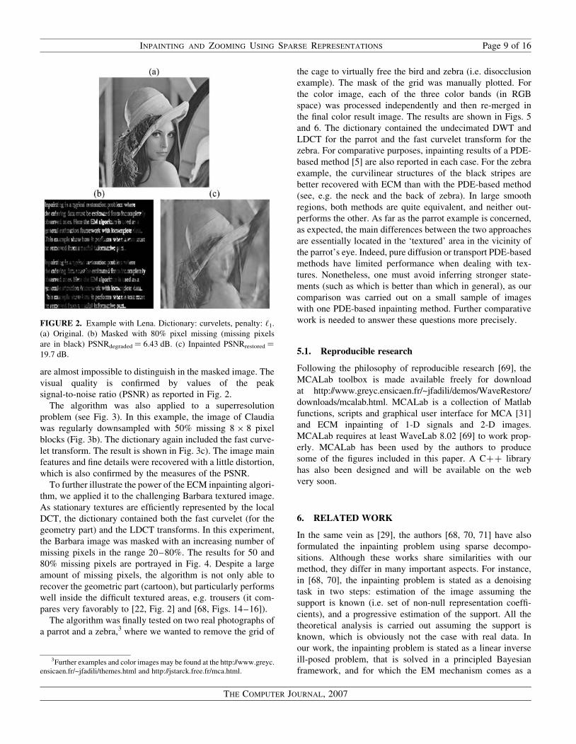
are almost impossible to distinguish in the masked image. The
visual quality is confirmed by values of the peak
signal-to-noise ratio (PSNR) as reported in Fig. 2.
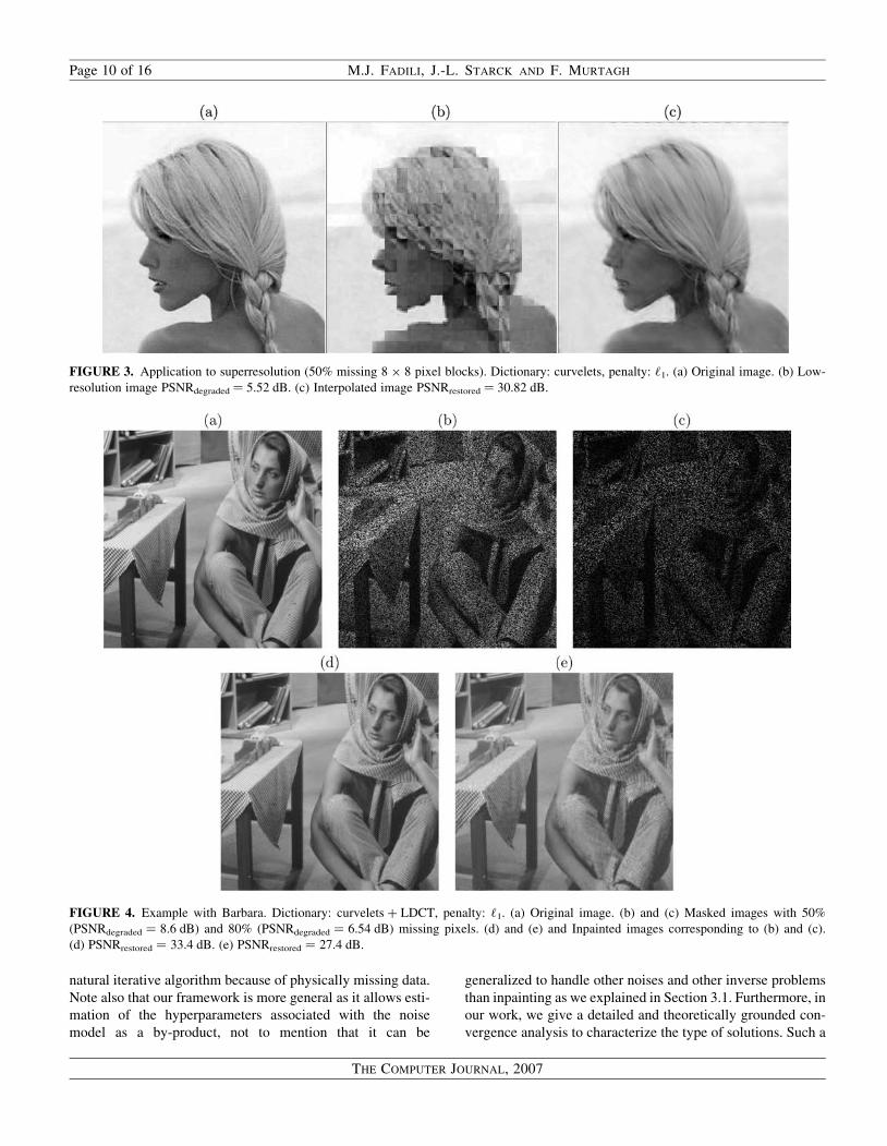
The algorithm was also applied to a superresolution
problem (see Fig. 3). In this example, the image of Claudia
was regularly downsampled with 50% missing 8 � 8 pixel
blocks (Fig. 3b). The dictionary again included the fast curve-
let transform. The result is shown in Fig. 3c). The image main
features and fine details were recovered with a little distortion,
which is also confirmed by the measures of the PSNR.
To further illustrate the power of the ECM inpainting algori-
thm, we applied it to the challenging Barbara textured image.
As stationary textures are efficiently represented by the local
DCT, the dictionary contained both the fast curvelet (for the
geometry part) and the LDCT transforms. In this experiment,
the Barbara image was masked with an increasing number of
missing pixels in the range 20–80%. The results for 50 and
80% missing pixels are portrayed in Fig. 4. Despite a large
amount of missing pixels, the algorithm is not only able to
recover the geometric part (cartoon), but particularly performs
well inside the difficult textured areas, e.g. trousers (it com-
pares very favorably to [22, Fig. 2] and [68, Figs. 14–16]).
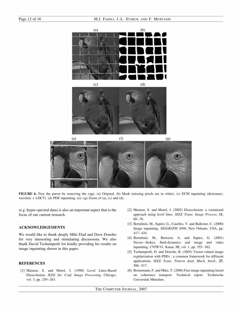
The algorithm was finally tested on two real photographs of
a parrot and a zebra,3 where we wanted to remove the grid of
the cage to virtually free the bird and zebra (i.e. disocclusion
example). The mask of the grid was manually plotted. For
the color image, each of the three color bands (in RGB
space) was processed independently and then re-merged in
the final color result image. The results are shown in Figs. 5
and 6. The dictionary contained the undecimated DWT and
LDCT for the parrot and the fast curvelet transform for the
zebra. For comparative purposes, inpainting results of a PDE-
based method [5] are also reported in each case. For the zebra
example, the curvilinear structures of the black stripes are
better recovered with ECM than with the PDE-based method
(see, e.g. the neck and the back of zebra). In large smooth
regions, both methods are quite equivalent, and neither out-
performs the other. As far as the parrot example is concerned,
as expected, the main differences between the two approaches
are essentially located in the ‘textured’ area in the vicinity of
the parrot’s eye. Indeed, pure diffusion or transport PDE-based
methods have limited performance when dealing with tex-
tures. Nonetheless, one must avoid inferring stronger state-
ments (such as which is better than which in general), as our
comparison was carried out on a small sample of images
with one PDE-based inpainting method. Further comparative
work is needed to answer these questions more precisely.
5.1. Reproducible research
Following the philosophy of reproducible research [69], the
MCALab toolbox is made available freely for download
at http://www.greyc.ensicaen.fr/~jfadili/demos/WaveRestore/
downloads/mcalab.html. MCALab is a collection of Matlab
functions, scripts and graphical user interface for MCA [31]
and ECM inpainting of 1-D signals and 2-D images.
MCALab requires at least WaveLab 8.02 [69] to work prop-
erly. MCALab has been used by the authors to produce
some of the figures included in this paper. A Cþþ library
has also been designed and will be available on the web
very soon.
6. RELATED WORK
In the same vein as [29], the authors [68, 70, 71] have also
formulated the inpainting problem using sparse decompo-
sitions. Although these works share similarities with our
method, they differ in many important aspects. For instance,
in [68, 70], the inpainting problem is stated as a denoising
task in two steps: estimation of the image assuming the
support is known (i.e. set of non-null representation coeffi-
cients), and a progressive estimation of the support. All the
theoretical analysis is carried out assuming the support is
known, which is obviously not the case with real data. In
our work, the inpainting problem is stated as a linear inverse
ill-posed problem, that is solved in a principled Bayesian
framework, and for which the EM mechanism comes as a
FIGURE 2. Example with Lena. Dictionary: curvelets, penalty: ‘1.
(a) Original. (b) Masked with 80% pixel missing (missing pixels
are in black) PSNRdegraded ¼ 6.43 dB. (c) Inpainted PSNRrestored ¼
19.7 dB.
3Further examples and color images may be found at the http://www.greyc.
ensicaen.fr/~jfadili/themes.html and http://jstarck.free.fr/mca.html.
INPAINTING AND ZOOMING USING SPARSE REPRESENTATIONS Page 9 of 16
THE COMPUTER JOURNAL, 2007
natural iterative algorithm because of physically missing data.
Note also that our framework is more general as it allows esti-
mation of the hyperparameters associated with the noise
model as a by-product, not to mention that it can be
generalized to handle other noises and other inverse problems
than inpainting as we explained in Section 3.1. Furthermore, in
our work, we give a detailed and theoretically grounded con-
vergence analysis to characterize the type of solutions. Such a
FIGURE 4. Example with Barbara. Dictionary: curvelets þ LDCT, penalty: ‘1. (a) Original image. (b) and (c) Masked images with 50%
(PSNRdegraded ¼ 8.6 dB) and 80% (PSNRdegraded ¼ 6.54 dB) missing pixels. (d) and (e) and Inpainted images corresponding to (b) and (c).
(d) PSNRrestored ¼ 33.4 dB. (e) PSNRrestored ¼ 27.4 dB.
FIGURE 3. Application to superresolution (50% missing 8 � 8 pixel blocks). Dictionary: curvelets, penalty: ‘1. (a) Original image. (b) Low-
resolution image PSNRdegraded ¼ 5.52 dB. (c) Interpolated image PSNRrestored ¼ 30.82 dB.
Page 10 of 16 M.J. FADILI, J.-L. STARCK AND F. MURTAGH
THE COMPUTER JOURNAL, 2007

convergence study is lacking in the work of [70, 71]. The
method in [70] can only handle dictionaries, which are
union of orthonormal bases, and the one in [71] proposes the
same algorithm as [70] with a dictionary formed by a single
tight frame (framelet). Our method seems to be more
general and naturally deals with any dictionary (union of trans-
forms that correspond to frames or tight frames such as the
curvelet transform). Hence, our algorithm can be used with
richer overcomplete dictionaries (beyond union of bases)
that are able to provide us with sparser representations of a
wide range of images based on their morphological content.
Additionally, we would like to make a connection with the
emerging theory which goes by the name of ‘compressive
sampling’ or ‘compressed sensing’ as recently developed by
Donoho [32] and Donoho and Tsiag [33] and Candes et al.
[34–36]. Roughly speaking, this theory establishes in a prin-
cipled way that it is possible to reconstruct images or signals
accurately from a number of samples which is far smaller
than the number of pixels in the image, if the image or signal
is sparse (compressible) enough in some dictionary. In fact,
accurate and sometimes exact recovery is possible by solving
a simple convex optimization problem. Such a theory, although
directed toward random sensing matrices, provides a theoreti-
cal justification as to why algorithms such as ours work so
well in an application such as image inpainting and zooming.
7. SUMMARY AND CONCLUSION
A novel and flexible inpainting algorithm has been presented.
Its theoretical properties were systematically investigated and
established in various scenarios. To demonstrate potential
applications of the algorithm, examples including inter-
polation, zooming (superresolution) and disocclusion were
considered. Several interesting perspectives of this work are
under investigation. We can cite the formal investigation of
the influence of the regularization parameter (path following/
homotopy continuation). Extension to multi-valued images
FIGURE 5. Free the zebra by removing the cage. (a) Original. (b) Mask (missing pixels are in white). (c) ECM inpainting (dictionary: curvelets).
(d) PDE inpainting.
INPAINTING AND ZOOMING USING SPARSE REPRESENTATIONS Page 11 of 16
THE COMPUTER JOURNAL, 2007
(e.g. hyper-spectral data) is also an important aspect that is the
focus of our current research.
ACKNOWLEDGEMENTS
We would like to thank deeply Miki Elad and Dave Donoho
for very interesting and stimulating discussions. We also
thank David Tschumperle for kindly providing his results on
image inpainting shown in this paper.
REFERENCES
[1] Masnou, S. and Morel, J. (1998) Level Lines-Based
Disocclusion. IEEE Int. Conf. Image Processing, Chicago,
vol. 3, pp. 259–263.
[2] Masnou, S. and Morel, J. (2002) Disocclusion: a variational
approach using level lines. IEEE Trans. Image Process, 11,
68–76.
[3] Bertalmıo, M., Sapiro, G., Caselles, V. and Ballester, C. (2000)
Image inpainting. SIGGRAPH 2000, New Orleans, USA, pp.
417–424.
[4] Bertalmıo, M., Bertozzi, A. and Sapiro, G. (2001)
Navier–Stokes, fluid-dynamics and image and video
inpainting. CVPR’01, Kauai, HI, vol. 1, pp. 355–362.
[5] Tschumperle, D. and Deriche, R. (2005) Vector-valued image
regularization with PDEs : a common framework for different
applications. IEEE Trans. Pattern Anal. Mach. Intell., 27,
506–517.
[6] Bornemann, F. and Marz, T. (2006) Fast image inpainting based
on coherence transport. Technical report. Technische
Universitat Munchen.
FIGURE 6. Free the parrot by removing the cage. (a) Original. (b) Mask (missing pixels are in white). (c) ECM inpainting (dictionary:
wavelets þ LDCT). (d) PDE inpainting. (e)–(g) Zoom of (a), (c) and (d).
Page 12 of 16 M.J. FADILI, J.-L. STARCK AND F. MURTAGH
THE COMPUTER JOURNAL, 2007
[7] Caselles, V., Morel, J. and Sbert, C. (1998) An axiomatic
approch to image interpolation. IEEE Trans. Image Process,
7, 376–386.
[8] Ballester, C., Caselles, V., Verdera, J., Sapiro, G. and Bertalmıo,
M. (2001) A Variational Model for Filling-in Gray Level and
Color Images. IEEE Int. Conf. Computer Vision, Vancouver,
Canada, pp. 10–16.
[9] Ballester, C., Bertalmıo, M., Caselles, V., Sapiro, G.
and Verdera, J. (2001) Filling-in by joint interpolation of
vector fields and gray levels. IEEE Trans. Image Process, 10,
1200–1211.
[10] Ballester, C., Caselles, V. and Verdera, J. (2003) Disocclusion
by joint interpolation of vector fields and gray levels.
Multiscale Modeling and Simul., 2, 80–123.
[11] Chan, T. and Shen, J. (2001) Non-texture inpainting by
curvature-driven diffusions (cdd). J. Vis. Commun. Image
Represent., 12, 436–449.
[12] Chan, T. and Shen, J. (2001) Mathematical models for local
non-texture inpainting. SIAM J. Appl. Math., 62, 1019–1043.
[13] Chan, T., Kang, S.H. and Shen, J. (2002) Euler’s elastica and
curvature based inpainting. SIAM J. Appl. Math., 63, 564–592.
[14] Esedoglu, S. and Shen, J. (2002) Digital image inpainting by the
Mumford-Shah-Euler image model. Eur. J. Appl. Math., 13,
353–370.
[15] Chan, T.F., Yip, A.M. and Park, F.E. (2004) Simultaneous total
variation image inpainting and blind deconvolution.
Int. J. Imaging Syst. Technol., 15, 92–102.
[16] Chan, T.F., Ng, M.K., Yau, A.C. and Yip, A.M. (2006)
Superresolution image reconstruction using fast inpainting
algorithms. Technical report. UCLA CAM.
[17] Song, B. (2003) Topics in Variational PDE Image
Segmentation, Inpainting and Denoising. PhD Thesis,
University of California, LA.
[18] Bertozzi, A., Esedoglu, S. and Gillette, A. (2007) Inpainting by
the Cahn-Hilliard equation. IEEE Trans. Image Process, 16,
285–291.
[19] Chan, T.F. and Shen, J.J. (2005) Image Processing and
Analysis-Variational, PDE, Wavelet, and Stochastic Methods.
SIAM, Philadelphia.
[20] Bertalmıo, M., Caselles, V., Haro, G. and Sapiro, G. (2005) The
State of the Art of Image and Surface Inpainting. In Paragios,
N., Faugeras, O. and Chen, Y. (eds.), Mathematical Models in
Computer Vision: The Handbook, pp. 309–322. Springer-
Verlag, Berlin.
[21] Efros, A.A. and Leung, T.K. (1999) Texture Synthesis by
Non-Parametric Sampling. IEEE Int. Conf. Computer Vision,
Kerkyra, Greece, pp. 1033–1038.
[22] Bertalmıo, M., Vese, L., Sapiro, G. and Osher, S. (2003)
Simultaneous structure and texture image inpainting. IEEE
Trans. Image Process, 12, 882–889.
[23] Demanet, L., Song, B. and Chan, T. (2003) Image Inpainting by
Correspondence Maps: A Deterministic Approach. VLSM, Nice,
France.
[24] Rane, S., Bertalmio, M. and Sapiro, G. (2002) Structure and
texture filling-in of missing image blocks for wireless
transmission and compression applications. IEEE Trans.
Image Process, 12, 296–303.
[25] Jia, J. and Tang, C.-K. (2003) Image Repairing: Robust Image
Synthesis By Adaptive Nd Tensor Voting. IEEE CVPR, vol. 1,
pp., 643–650.
[26] Acton, S.T., Mukherjee, D.P., Havlicek, J.P. and Bovik, A.C.
(2001) Oriented texture completion by AM-FM
reaction-diffusion. IEEE Trans. Image Process, 10, 885–896.
[27] Criminisi, A., Perez, P. and Toyama, K. (2004) Region filling
and object removal by examplar-based image inpainting.
IEEE Trans. Image Process, 13, 1200–1212.
[28] Drori, I., Cohen-Or, D. and Yeshurun, H. (2003) Fragment-based
image completion. ACM Trans. Graph., 22, 303–312.
[29] Elad, M., Starck, J.-L., Querre, P. and Donoho, D. (2005)
Simultaneous cartoon and texture image inpainting. Appl.
Comput. Harmon. Anal., 19, 340–358.
[30] Starck, J.-L., Elad, M. and Donoho, D. (2005) Image
decomposition via the combination of sparse representatntions
and variational approach. IEEE Trans. Image Process, 14,
1570–1582.
[31] Starck, J.-L., Elad, M. and Donoho, D. (2004) Redundant
multiscale transforms and their application for morphological
component analysis. Adv. Imag. Electron Phys., 132, 287–348.
[32] Donoho, D.L. (2004) Compressed sensing. Technical report.
Stanford University, Department of Statistics.
[33] Donoho, D. and Tsaig, Y. (2006) Extensions of compressed
sensing. EURASIP J. Appl. Signal Process., 86, 549–571.
[34] Candes, E., Romberg, J. and Tao, T. (2004) Robust uncertainty
principles: Exact signal reconstruction from highly incomplete
frequency information. Technical report. CalTech, Applied
and Computational Mathematics.
[35] Candes, E. and Tao, T. (2005) Stable signal recovery from noisy
and incomplete observations. Technical report. CalTech,
Applied and Computational Mathematics.
[36] Candes, E. and Tao, T. (2004) Near optimal signal recovery from
random projections: universal encoding strategies? Technical
report. CalTech, Applied and Computational Mathematics.
[37] Dempster, A., Laird, N. and Rubin, D. (1977) Maximum
likelihood from incomplete data via the EM algorithm. J. Roy.
Stat. Soc. B, 39, 1–38.
[38] Little, R. and Rubin, D. (1987) Statistical Analysis with Missing
Data. Wiley, New York.
[39] Mallat, S.G. (1998) A Wavelet Tour of Signal Processing (2nd
edn). Academic Press.
[40] Starck, J.-L., Murtagh, F. and Bijaoui, A. (1998) Image
Processing and Data Analysis: The Multiscale Approach.
Cambridge University Press.
[41] Candes, E.J. and Donoho, D.L. (1999) Curvelets—a
surprisingly effective nonadaptive representation for objects
with edges. In Cohen, A., Rabut, C. and Schumaker, L. (eds.),
Curve and Surface Fitting: Saint-Malo 1999, Vanderbilt
University Press, Nashville, TN.
[42] Candes, E., Demanet, L., Donoho, D. and Ying, L. (2006) Fast
discrete curvelet transforms. SIAM Multiscale Modeling Simul.,
5, 861–899.
INPAINTING AND ZOOMING USING SPARSE REPRESENTATIONS Page 13 of 16
THE COMPUTER JOURNAL, 2007
[43] Candes, E. and Donoho, D. (1999) Ridgelets: the key to high
dimensional intermittency? Philos. Trans. R. Soc. Lond. A,
357, 2495–2509.
[44] Starck, J.L., Candes, E. and Donoho, D.L. (2002) The curvelet
transform for image denoising. IEEE Trans. Image Process, 11,
670–684.
[45] Donoho, D. and Elad, M. (2003) Optimally sparse
representation in general (non-orthogonal) dictionaries via ‘1
minimization. Proc. Natl Acad. Sci., 100, 2197–2202.
[46] Bruckstein, A. and Elad, M. (2002) A generalized uncertainty
principle and sparse representation in pairs of RN bases. IEEE
Trans. Inf. Theory, 48, 2558–2567.
[47] Gribonval, R. and Nielsen, M. (2003) Sparse representations in
unions of bases. IEEE Trans. Inf. Theory, 49, 3320–3325.
[48] Tropp, T. (2004) Topics in sparse approximation. PhD Thesis,
University of Texas, Austin.
[49] Bickel, P. and Docksum, K. (2001) Mathematical Statistics: Basic
Ideas and Selected Topics (2nd edn). Prentice-Hall, London.
[50] Chen, S.S., Donoho, D.L. and Saunders, M.A. (1999) Atomic
decomposition by basis pursuit. SIAM J. Sci. Comput., 20, 33–61.
[51] Sardy, S., Bruce, A. and Tseng, P. (2000) Block coordinate
relaxation methods for nonparametric wavelet denoising.
J. Comput. Graph. Stat., 9, 361–379.
[52] Antoniadis, A. and Fan, J. (2001) Regularization of wavelets
approximations. J. Am. Stat. Assoc., 96, 939–963.
[53] Nikolova, M. (2000) Local strong homogeneity of a regularized
estimator. SIAM J. Appl. Math., 61, 633–658.
[54] Elad, M. (2005) Why simple shrinkage is still relevant for
redundant representations? Technical report. Department of
Computer Science, Technion.
[55] Elad, M., Matalon, B. and Zibulevsky, M. (2006) Coordinate
and subspace optimization methods for linear least squares
with non-quadratic regularization. Technical report.
Department of Computer Science, Technion.
[56] Meng, X.L. and Rubin, D.B. (1993) Maximum likelihood
estimation via the ECM algorithm: a general framework.
Biometrika, 80, 267–278.
[57] Wu, C. (1983) On the convergence properties of the EM
algorithm. Ann. Stat., 11, 95–103.
[58] Nikolova, M. (2005) Analysis of the recovery of edges in
images and signals by minimizing nonconvex regularized
least-squares. SIAM J. Multiscale Modeling Simul., 4, 960–991.
[59] Combettes, P.L. and Wajs, V.R. (2005) Signal recovery by
proximal forward-backward splitting. SIAM J. Multiscale
Modeling Simul., 4, 1168–1200.
[60] Meng, X.L. and Rubin, D.B. (1992) Recent extensions to the
EM algorithm. In Bernardo, J., Berger, J., Dawid, A.
and Smith, A. (eds.), Bayesian Statistics, pp. 307–320.
Oxford University Press.
[61] Meng, X.L. (1994) On the rate of convergence of the ECM
algorithm. Ann. Stat., 22, 326–339.
[62] Ciarlet, P.G. (1982) Introduction a l’Analyse Numerique
Matricielle et a l’Optimisation. Masson, Paris.
[63] Glowinski, R., Lions, J. and Tremolieres, R. (1976) Analyse
NumeriquedesInequationsVariationnelles(1stedn).Dunod,Paris.
[64] Tseng, P. (2001) Convergence of a block coordinate descent
method for nondifferentiable minimizations. J. Optim. Theory
Appl., 109, 457–494.
[65] Ueda, N. and Nakano, R. (1998) Deterministic annealing EM
algorithm. Neural Netw., 11, 271–282.
[66] Efron, B., Hastie, T., Johnstone, I. and Tibshirani, R. (2004)
Least angle regression. Ann. Stat., 32, 407–499.
[67] Donoho, D., Tsaig, Y., Drori, I. and Starck, J.-K. (2006) Sparse
solution of underdetermined linear equations of stagewise
orthogonal matching pursuit. Technical Report. Dept. of
Statistics, Stanford University.
[68] Guleryuz, O. (2006) Nonlinear approximation based image
recovery using adaptive sparse reconstructions and iterated
denoising. Part II: adpative algorithms. IEEE Trans. Image
Process, 15, 555–571.
[69] Buckheit, J. and Donoho, D. (1995) Wavelab and Reproducible
Research. In Antoniadis, A. (ed.), Wavelets and Statistics.
Springer.
[70] Guleryuz, O. (2006) Nonlinear approximation based image
recovery using adaptive sparse reconstructions and iterated
denoising. Part I: theory. IEEE Trans. Image Process, 15, 539–554.
[71] Chan, R., Shen, L. and Shen, Z. (2005) A framelet-based
approach for image inpainting. Technical report. The Chinese
University of Hong Kong.
[72] Opial, Z. (1967) Weak convergence of the sequence of
successive approximations for nonexpansive mappings. Bull.
Am. Math. Soc., 73, 591–597.
[73] Daubechies, I., Defrise, M. and Mol, C.D. (2004) An iterative
thresholding algorithm for linear inverse problems with a
sparsity constraint. Comm. Pure Appl. Math., 57, 1413–1541.
8. APPENDIX
8.1. Proof of Proposition 1
Proof. Proof of (i) follows the same lines as in [52, 53]. When
F is a basis, the solution to Equation (6) is a componentwise
minimization problem. When z ¼ 0, it is clear that the unique
minimizer is a ¼ 0. Moreover, as the functional to be mini-
mized is even-symmetric (owing to H), the solution function
is odd, i.e. a(2z) ¼ 2a(z). Thus, we study the problem
only for z . 0. By differentiating (using H3), we have
a ¼ z� ls2c0ðaÞ: ðA:1Þ
Using a simple contradiction argument, a and z necessarily
have the same sign. Indeed, assume that a � 0 when z . 0.
But, by H1, the right-hand side of Equation (A.1) is positive,
contradicting our initial assumption. Thus, if z � minb�0
b þ ls2c 0(b) ¼ T, the only positive solution to Equation
(A.1) is a ¼ 0. On the other hand, when z . T, Equation
(A.1) may have many solutions. For c convex, it is trivial to
see that a þ ls2c 0(a) is one-to-one for z . T, hence the solu-
tion is unique. Otherwise, owing to H4, the componentwise
derivative written in Equation (A.1) has two possible zero
Page 14 of 16 M.J. FADILI, J.-L. STARCK AND F. MURTAGH
THE COMPUTER JOURNAL, 2007

crossings on (0, þ 1), but only the larger one is the minimum
occurring at a strictly positive a. Finally, to ensure continuity
of a(z) at T, T is necessarily ls2c 0þ(0).
Assertions (ii) and (iii) follow as a direct application of [57,
Theorem 2], as since the surrogate functional Q(aja(t)) is con-
tinuous in both arguments (see H3). A
8.2. Proof of Proposition 2
Proof. Existence statement (i) is a consequence of coercivity,
which is a sufficient condition for the inpainting problem to
have a solution.
Uniqueness assertion (ii) follows as a consequence of [59,
Proposition 5.15(ii)(a)], as MF is not necessarily bounded
below.
To prove (iii), let us define the sequence of iterates
xðtþ1Þ ¼ DF;l yobs þ ðI�MÞxðtÞ
� �; ðA:2Þ
where DF,l ¼ FSls2FT consists of applying the transform
T ¼ FT, the componentwise shrinkage operator associated
with Equation (14) with a parameter ls2, and then reconstruct.
LEMMA 1. If c 0(.) is non-decreasing, DF,l is a non-
expansive operator.
Proof. Since the ‘2-norm is invariant under orthonormal
transformations (F), it is sufficient to prove that, 8 z, z0 [ R
jaðzÞ � a0ðz0Þj � jz� z0j: ðA:3Þ
This is just checked in all possible cases.
(i) If jzj � T and jz0j � T, ja(z) 2 a0(z0)j ¼ 0 � j z 2 z0j.
(ii) Conversely, consider z and z0 to have the same sign and
jzj. T and jz0j . T, the function z(a) ¼ a þ ls2c 0(a)
is one-to-one monotonically increasing with derivative
uniformly bounded below by 1, hence verifying
Equation (A.3).
(iii) If z . T and z0 ,2T, ja(z) 2 a0(z0)j ¼ jz 2 z0 2
ls2(c 0(a) 2 c 0(a0))j, jz 2 z0j.
(iv) If z . T and jz0j, T, by monotonicity of c 0:
jaðzÞj � a0ðz0Þj ¼ jz� ls2c0ðaÞj
� jz� ls2c0þð0Þj
� jz� z0j: ðA:4Þ
A
It is now straightforward to see that
kxðtþ1Þ � xðtÞk2 � k I�Mð ÞðxðtÞ � xðt�1ÞÞk2
, kxðtÞ � xðt�1Þk2: ðA:5Þ
The last strict inequality holds whenever some data is missing
(i.e. avoiding the trivial identity mask). Furthermore, by stan-
dard properties of the EM (see Proposition 1(ii)), Q(x (tþ1)jx (t))
and the penalized log-likelihood ‘c increase monotonically.
Therefore, from the definition of the surrogate functional
Q(.j.) in Equation (9):
Qðxðtþ1ÞjxðtÞÞ ¼ ‘‘ðyojxðtþ1ÞÞ � lC FTxðtþ1Þ
� ��
1
2s2I�MÞð xðtþ1Þ � xðtÞ
� � 2
2
¼ ‘‘cðyojxðtþ1ÞÞ
�1
2s2I�MÞð xðtþ1Þ � xðtÞ
� � 2
2
� QðxðtÞjxðtÞÞ ¼ ‘‘cðyojxðtÞÞ: ðA:6Þ
Thus,
XN
t¼0
ðI�MÞ xðtþ1Þ � xðtÞ� � 2
2
� 2s2XN
t¼0
‘‘cðyojxðtþ1ÞÞ � ‘‘cðyojx
ðtÞÞ� �
� 2s2 ‘‘cðyojxðNÞÞ � ‘‘cðyojx
ð0ÞÞ� �
� �2s2‘‘cðyojxð0ÞÞ , þ1: ðA:7Þ
It follows that the seriesP
t¼0Nkx (tþ1) 2 x (t)
k22 is bounded uni-
formly in N, so thatP
t¼01kx (tþ1) 2 x (t)
k22 converges. Thus,
the sequence of iterates is asymptotically regular. Finally, as
the set of fixed points is non-empty (coercivity), DF,l is non-
expansive and the sequence x (t) is asymptotically regular. By
application of Opial’s theorem [72], statement (iii) follows.
The proof provided here bears similarities with the one
given in [73].
To prove statement (iv), it is sufficient to identify our
problem with the one considered by Combettes and Wajs
[59, Problem 5.13], and their fixed-point iteration [59, Pro-
blems (5.24) and (5.25)] with ours. It turns out that the shrink-
age operator Sls2 in Equation (14) is the Moreau proximity
operator associated with the convex function c, the lossy
operatorM is a bounded linear operator, and F is a bijective
bounded linear operator. Thus, strong convergence follows
from [59, Corollary 5.19]. A
8.3. Proof of Proposition 3
Proof. The proof for frames is less straightforward that for a
basis. To prove our result, we invoke a theorem due to [59,
Theorem 5.5]. For the sake of completeness and the reader’s
convenience, we here state in full some of their results relevant
to our setting, but without a proof.
INPAINTING AND ZOOMING USING SPARSE REPRESENTATIONS Page 15 of 16
THE COMPUTER JOURNAL, 2007
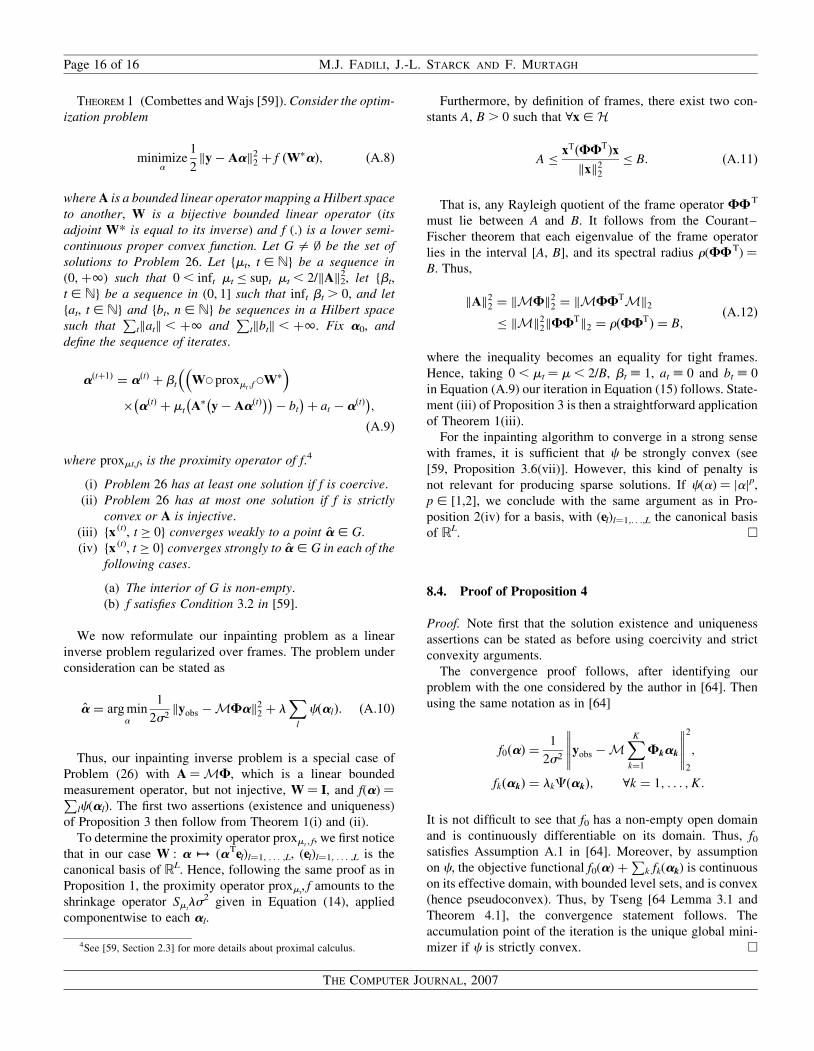
THEOREM 1 (Combettes and Wajs [59]). Consider the optim-
ization problem
minimizea
1
2ky� Aak2
2 þ f ðWaÞ; ðA:8Þ
where A is a bounded linear operator mapping a Hilbert space
to another, W is a bijective bounded linear operator (its
adjoint W* is equal to its inverse) and f (.) is a lower semi-
continuous proper convex function. Let G = ; be the set of
solutions to Problem 26. Let fmt, t [ Ng be a sequence in
(0, þ1) such that 0 , inft mt � supt mt , 2/kAk22, let fbt,
t [ Ng be a sequence in (0, 1] such that inft bt . 0, and let
fat, t [ Ng and fbt, n [ Ng be sequences in a Hilbert space
such thatP
tkatk , þ1 andP
tkbtk, þ1. Fix a0, and
define the sequence of iterates.
aðtþ1Þ ¼ aðtÞ þ bt WW proxmt;fWW
�� aðtÞ þ mt A y� AaðtÞ
� �� �� bt
� �þ at � aðtÞ
�;
ðA:9Þ
where proxmt,f, is the proximity operator of f.4
(i) Problem 26 has at least one solution if f is coercive.
(ii) Problem 26 has at most one solution if f is strictly
convex or A is injective.
(iii) fx (t), t � 0g converges weakly to a point a [ G.
(iv) fx (t), t � 0g converges strongly to a [ G in each of the
following cases.
(a) The interior of G is non-empty.
(b) f satisfies Condition 3.2 in [59].
We now reformulate our inpainting problem as a linear
inverse problem regularized over frames. The problem under
consideration can be stated as
a ¼ arg mina
1
2s2kyobs �MFak22 þ l
Xl
cðalÞ: ðA:10Þ
Thus, our inpainting inverse problem is a special case of
Problem (26) with A ¼MF, which is a linear bounded
measurement operator, but not injective, W ¼ I, and f(a) ¼Plc(al). The first two assertions (existence and uniqueness)
of Proposition 3 then follow from Theorem 1(i) and (ii).
To determine the proximity operator proxmt , f, we first notice
that in our case W : a 7! (aTel)l¼1, . . . ,L, (el)l¼1, . . . ,L is the
canonical basis of RL. Hence, following the same proof as in
Proposition 1, the proximity operator proxmt, f amounts to the
shrinkage operator Smtls2 given in Equation (14), applied
componentwise to each al.
Furthermore, by definition of frames, there exist two con-
stants A, B . 0 such that 8x [H
A �xTðFFT
Þx
kxk22� B: ðA:11Þ
That is, any Rayleigh quotient of the frame operator FFT
must lie between A and B. It follows from the Courant–
Fischer theorem that each eigenvalue of the frame operator
lies in the interval [A, B], and its spectral radius r(FFT) ¼
B. Thus,
kAk22 ¼ kMFk22 ¼ kMFFT
Mk2
� kMk22kFFTk2 ¼ rðFFT
Þ ¼ B;ðA:12Þ
where the inequality becomes an equality for tight frames.
Hence, taking 0 , mt ¼ m , 2/B, bt ; 1, at ; 0 and bt ; 0
in Equation (A.9) our iteration in Equation (15) follows. State-
ment (iii) of Proposition 3 is then a straightforward application
of Theorem 1(iii).
For the inpainting algorithm to converge in a strong sense
with frames, it is sufficient that c be strongly convex (see
[59, Proposition 3.6(vii)]. However, this kind of penalty is
not relevant for producing sparse solutions. If c(a) ¼ jajp,
p [ [1,2], we conclude with the same argument as in Pro-
position 2(iv) for a basis, with (el)l¼1,. . .,L the canonical basis
of RL. A
8.4. Proof of Proposition 4
Proof. Note first that the solution existence and uniqueness
assertions can be stated as before using coercivity and strict
convexity arguments.
The convergence proof follows, after identifying our
problem with the one considered by the author in [64]. Then
using the same notation as in [64]
f0ðaÞ ¼1
2s2yobs �M
XK
k¼1
Fkak
2
2
;
fkðakÞ ¼ lkCðakÞ; 8k ¼ 1; . . . ;K:
It is not difficult to see that f0 has a non-empty open domain
and is continuously differentiable on its domain. Thus, f0satisfies Assumption A.1 in [64]. Moreover, by assumption
on c, the objective functional f0(a) þP
k fk(ak) is continuous
on its effective domain, with bounded level sets, and is convex
(hence pseudoconvex). Thus, by Tseng [64 Lemma 3.1 and
Theorem 4.1], the convergence statement follows. The
accumulation point of the iteration is the unique global mini-
mizer if c is strictly convex. A4See [59, Section 2.3] for more details about proximal calculus.
Page 16 of 16 M.J. FADILI, J.-L. STARCK AND F. MURTAGH
THE COMPUTER JOURNAL, 2007


![0804 EAV (CFA610)[1]](https://img.pdfslide.us/doc/110x75/577d39a41a28ab3a6b9a3fc6/0804-eav-cfa6101.jpg)