Meta-programming with Names and Necessity

Aleksandar Nanevski

November 2002CMU-CS-02-123R

School of Computer ScienceCarnegie Mellon University

Pittsburgh, PA 15213

This report is a significant revision of and supersedes the version published in April 2002 under the

number CMU-CS-02-123

Abstract

Meta-programming is a discipline of writing programs in a certain programming language that generate,manipulate or execute programs written in another language. In a typed setting, meta-programming lan-guages usually contain a modal type constructor to distinguish the level of object programs (which are themanipulated data) from the meta programs (which perform the computations). In functional programming,modal types of object programs generally come in two flavors: open and closed, depending on whether theexpressions they classify may contain any free variables or not. Closed object programs can be executedat run-time by the meta program, but the computations over them are more rigid, and typically produceless efficient residual code. Open object programs provide better inlining and partial evaluation, but onceconstructed, expressions of open modal type cannot be evaluated.Recent work in this area has focused on combining the two notions into a sound type system. We present anovel calculus to achieve this, which we call ν�. It is based on adding the notion of names inspired by thework on Nominal Logic and FreshML to the λ�-calculus of proof terms for the necessity fragment of modallogic S4. The resulting language provides a more fine-grained control over free variables of object programswhen compared to the existing languages for meta-programming. In addition, we extend our calculus withprimitives for inspection and destruction of object programs at run-time in a type-safe manner.

Keywords: meta-programming, modal logic, nominal logic, higher-order abstract syntax, staged com-putation, run-time code generation, symbolic computation

Contents

1 Introduction 1

2 Modal λ�-calculus 3

3 Modal calculus of names 43.1 Motivation, syntax and overview . . . . . . . . . . . . . . . . . . . . . . . . . . . . . . . . . . 43.2 Explicit substitutions . . . . . . . . . . . . . . . . . . . . . . . . . . . . . . . . . . . . . . . . . 83.3 Type system . . . . . . . . . . . . . . . . . . . . . . . . . . . . . . . . . . . . . . . . . . . . . 93.4 Structural properties . . . . . . . . . . . . . . . . . . . . . . . . . . . . . . . . . . . . . . . . . 123.5 Operational semantics . . . . . . . . . . . . . . . . . . . . . . . . . . . . . . . . . . . . . . . . 15

4 Support polymorphism 16

5 Intensional analysis of higher-order syntax 185.1 Syntax and typechecking . . . . . . . . . . . . . . . . . . . . . . . . . . . . . . . . . . . . . . . 185.2 Operational semantics . . . . . . . . . . . . . . . . . . . . . . . . . . . . . . . . . . . . . . . . 20

6 Related work 23

7 Conclusions and future work 25

8 Acknowledgment 26

Bibliography 26

A Proofs 28A.1 Structural properties . . . . . . . . . . . . . . . . . . . . . . . . . . . . . . . . . . . . . . . . . 28A.2 Substitution principles . . . . . . . . . . . . . . . . . . . . . . . . . . . . . . . . . . . . . . . . 30A.3 Operational semantics . . . . . . . . . . . . . . . . . . . . . . . . . . . . . . . . . . . . . . . . 35A.4 Intensional analysis of higher-order syntax . . . . . . . . . . . . . . . . . . . . . . . . . . . . . 37

1 Introduction

Meta-programming is a paradigm referring to the ability to algorithmically compose programs of a certainobject language, through a program written in a meta-language. A particularly intriguing instance of thisconcept, and the one we are interested in in this work, is when the meta and the object language are: (1)the same, or the object language is a subset of the meta language; and (2) typed functional languages. Alanguage satisfying (1) adds the possibility to also invoke the generated programs at run-time. We refer tothis setup as homogeneous meta-programming.

Among some of the advantages of meta-programming and of its homogeneous and typed variant wedistinguish the following (and see [She01] for a comprehensive analysis).

Efficiency. Rather than using one general procedure to solve many different instances of a problem, aprogram can generate specialized (and hence more efficient) subroutines for each particular case. If thelanguage is capable of executing thus generated procedures, the program can choose dynamically, dependingon a run-time value of a certain variable or expression, which one is most suitable to invoke. This is the ideabehind the work on run-time code generation [LL96, WLP98, WLPD98] and the functional programmingconcept of staged computation [DP01].

Maintainability. Instead of maintaining a number of specialized, but related, subprograms, it is easier tomaintain their generator. In a language capable of invoking the generated code, there is an added bonus ofbeing able to accentuate the relationship between the synthesized code and its producer; the subroutines canbe generated and bound to their respective identifiers in the initialization stage of the program execution,rather then generated and saved into a separate file of the build tree for later compilation and linking.

1

Languages in which object programs can not only be composed and executed but also have their structureinspected add further advantages. Efficiency benefits from various optimizations that can be performedknowing the structure of the code. For example, Griewank reports in [Gri89] on a way to reuse commonsubexpressions of a numerical function in order to compute its value at a certain point and the value of itsn-dimensional gradient, but in such a way that the complexity of both evaluations performed together doesnot grow with n. Maintainability (and in general the whole program development process) benefits from thepresence of types on both the level of synthesized code, and on the level of program generators. Finally, thereare applications from various domains, which seem to call for the capability to execute a certain functionas well as recurse over its structure: see [Roz93] for examples in computer graphics and numerical analysis,and [RP02] for an example in machine learning and probabilistic modeling.

Recent developments in type systems for meta-programming have been centered around two particularmodal lambda calculi: λ� and λ©. The λ�-calculus is the proof-term language for the modal logic S4,whose necessity constructor � annotates valid propositions [DP01, PD01]. The type �A has been used inrun-time code generation to classify generators of code of type A [WLP98, WLPD98]. The λ©-calculus isthe proof-term language for discrete linear temporal logic, and the type ©A classifies terms associated withthe subsequent time moment. The intended application of λ© is in partial evaluation because the typingannotation of a λ©-program can be seen as its binding-time specification [Dav96]. Both calculi provide adistinction between levels (or stages) of terms, and this explains their use in meta-programming. The lowest,level 0, is the meta language, which is used to manipulate the terms on level 1 (terms of type �A in λ�

and ©A in λ©). This first level is the meta language for the level 2 containing another stratum of boxedand circled types, etc. For purposes of meta-programming, the type �A is also associated with closed code– it classifies closed object terms of type A. On the other hand, the type ©A is the type of postponed code,because it classifies object terms of type A which are associated with the subsequent time moment. Theimportant property of λ© is that its terms at a certain temporal level n may refer to variables which are onthe same temporal level n. Because these variables can be predeclared in the context, the postponed codetype of λ© is frequently conflated with the notion of open code. The abstract concept of open code (notnecessarily that of λ©) is obviously more general than that of closed code, and it is certainly desirable toendow a meta-programming language with it. As already observed in [Dav96] in the context of λ©, workingwith open code is more flexible and results in better and more optimized residual programs. However, wealso want to run the generated object programs when they are closed, and unfortunately, the modal type ofλ© does not provide for this.

There have been several proposed type systems which incorporate the the advantages from both languages,most notable being MetaML [MTBS99, Tah99, CMT00, CMS01]. MetaML defines its notion of open codeto be that of the postponed code of λ© and then introduces closed code as a refinement – as open codewhich happens to contain no free variables. Our calculus, which we call ν�, has the opposite approach.Rather than refining the notion of postponed code of λ©, we relax the notion of closed code of λ�. We startwith the system of λ�, but provide the additional expressiveness by allowing the code to contain specifiedobject variables as free (and rudiments of this idea have already been considered in [Nie01]). The fact thata given code expression depends on a set of free variables will be reflected in its type. The object variablesthemselves are represented by a separate semantic category of names (also called symbols or atoms), whichadmits equality. The treatment of names is inspired by the work on Nominal Logic and FreshML by Pitts andGabbay [GP02, PG00, Pit01, Gab00]. This design choice lends itself well to the addition, in an orthogonalway, of intensional code analysis, which we also undertake for a fragment of our language. Thus, we can alsotreat our object expressions as higher-order syntactic data; they can not only be evaluated, but can also becompared for structural equality and destructed via pattern-matching, much in the same way as one wouldwork with any abstract syntax tree.

The rest of the document is organized as follows: Section 2 is a brief exposition of the previous workon λ�. The type system of ν� and its properties are described in Section 3, while Section 4 describesparametric polymorphism in sets of names. Intensional analysis of higher-order syntax is introduced inSection 5. Finally, we illustrate the type system with example programs, before discussing the related workin Section 6. This paper supersedes the previously published [Nan02].

2

2 Modal λ�-calculus

This section reviews the previous work on the modal λ�-calculus and its use in meta-programming toseparate, through the mechanism of types, the realms of meta-level programs and object-level programs.The λ�-calculus is the proof-term calculus for the necessitation fragment of modal logic S4 [PD01, DP01].Chronologically, it came to be considered in functional programming in the context of specialization forpurposes of run-time code generation [WLP98, WLPD98]. For example, consider the exponentiation function,presented below in ML-like notation.

fun exp1 (n : int) (x : int) : int =if n = 0 then 1 else x * exp1 (n-1) x

The function exp1 : int -> int -> int is written in curried form so that it can be applied when only apart of its input is known. For example, if an actual parameter for n is available, exp1(n) returns a functionfor computing the n-th power of its argument. In a practical implementation of this scenario, however, theoutcome of the partial instantiation will be a closure waiting to receive an actual parameter for x before itproceeds with evaluation. Thus, one can argue that the following reformulation of exp1 is preferable.

fun exp2 (n : int) : int -> int =if n = 0 then λx:int.1else

let val u = exp2 (n - 1)in

λx:int. x * u(x)end

Indeed, when only n is provided, but not x, the expression exp2(n) performs computation steps based onthe value of n to produce a residual function specialized for computing the n-th power of its argument. Inparticular, the obtained residual function will not perform any operations or take decisions at run-time basedon the value of n; in fact, it does not even depend on n – all the computation steps dependent on n havebeen taken during the specialization.

A useful intuition for understanding the programming idiom of the above example, is to view exp2 as aprogram generator; once supplied with n, it generates the specialized function for computing n-th powers.This immediately suggests a distinction in the calculus between two stages (or levels): the meta and theobject stage. The object stage of an expression encodes λ-terms that are to be viewed as data – as results of aprocess of code generation. In the exp2 function, such terms would be (λx:int.1) and (λx:int. x * u(x)).The meta stage describes the specific operations to be performed over the expressions from the object stage.This is why the above-illustrated programming style is referred to as staged computation.

The idea behind the type system of λ� is to make explicit the distinction between meta and object stages.It allows the programmer to specify the intended staging of a term by annotating object-level subterms of theprogram. Then the type system can check whether the written code conforms to the staging specifications,making staging errors into type errors. The syntax of λ� is presented below.

Types A : : = b | A1 → A2 | �ATerms e : : = c | x | u | λx:A. e | e1 e2 | box e | let box u = e1 in e2

V alue variable contexts Γ : : = · | Γ, x:AExpression variable contexts ∆ : : = · | ∆, u:AV alues v : : = c | λx:A. e | box e

There are several distinctive features of the calculus, arising from the desire to differentiate between thestages. The most important is the new type constructor �. It is usually referred to as modal necessity, as onthe logic side it is a necessitation modifier on propositions [PD01]. In our meta-programming application, itis used to classify object-level terms. Its introduction and elimination forms are the term constructors boxand let box, respectively. If e is an object term of type A, then box e would be a meta term of type �A.The box term constructor encases the object term e so that it can be accessed and manipulated by the metapart of the program. The elimination form let box u = e1 in e2 does the opposite; it takes the object term

3

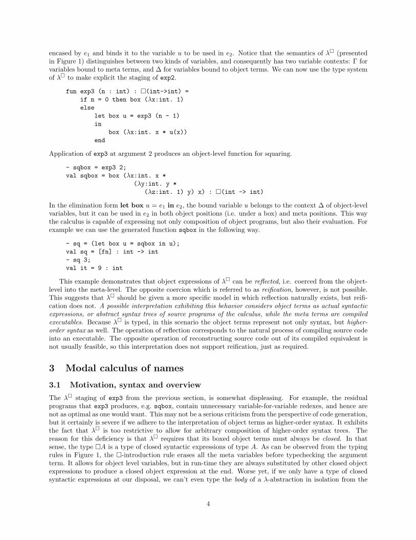
encased by e1 and binds it to the variable u to be used in e2. Notice that the semantics of λ� (presentedin Figure 1) distinguishes between two kinds of variables, and consequently has two variable contexts: Γ forvariables bound to meta terms, and ∆ for variables bound to object terms. We can now use the type systemof λ� to make explicit the staging of exp2.

fun exp3 (n : int) : �(int->int) =if n = 0 then box (λx:int. 1)else

let box u = exp3 (n - 1)in

box (λx:int. x * u(x))end

Application of exp3 at argument 2 produces an object-level function for squaring.

- sqbox = exp3 2;val sqbox = box (λx:int. x *

(λy:int. y *(λz:int. 1) y) x) : �(int -> int)

In the elimination form let box u = e1 in e2, the bound variable u belongs to the context ∆ of object-levelvariables, but it can be used in e2 in both object positions (i.e. under a box) and meta positions. This waythe calculus is capable of expressing not only composition of object programs, but also their evaluation. Forexample we can use the generated function sqbox in the following way.

- sq = (let box u = sqbox in u);val sq = [fn] : int -> int- sq 3;val it = 9 : int

This example demonstrates that object expressions of λ� can be reflected, i.e. coerced from the object-level into the meta-level. The opposite coercion which is referred to as reification, however, is not possible.This suggests that λ� should be given a more specific model in which reflection naturally exists, but reifi-cation does not. A possible interpretation exhibiting this behavior considers object terms as actual syntacticexpressions, or abstract syntax trees of source programs of the calculus, while the meta terms are compiledexecutables. Because λ� is typed, in this scenario the object terms represent not only syntax, but higher-order syntax as well. The operation of reflection corresponds to the natural process of compiling source codeinto an executable. The opposite operation of reconstructing source code out of its compiled equivalent isnot usually feasible, so this interpretation does not support reification, just as required.

3 Modal calculus of names

3.1 Motivation, syntax and overview

The λ� staging of exp3 from the previous section, is somewhat displeasing. For example, the residualprograms that exp3 produces, e.g. sqbox, contain unnecessary variable-for-variable redexes, and hence arenot as optimal as one would want. This may not be a serious criticism from the perspective of code generation,but it certainly is severe if we adhere to the interpretation of object terms as higher-order syntax. It exhibitsthe fact that λ� is too restrictive to allow for arbitrary composition of higher-order syntax trees. Thereason for this deficiency is that λ� requires that its boxed object terms must always be closed. In thatsense, the type �A is a type of closed syntactic expressions of type A. As can be observed from the typingrules in Figure 1, the �-introduction rule erases all the meta variables before typechecking the argumentterm. It allows for object level variables, but in run-time they are always substituted by other closed objectexpressions to produce a closed object expression at the end. Worse yet, if we only have a type of closedsyntactic expressions at our disposal, we can’t even type the body of a λ-abstraction in isolation from the

4

Typechecking

x:A ∈ Γ

∆; Γ ` x : A

u:A ∈ ∆

∆; Γ ` u : A

∆; (Γ, x:A) ` e : B

∆; Γ ` λx:A. e : A→ B

∆; Γ ` e1 : A→ B ∆; Γ ` e2 : A

∆; Γ ` e1 e2 : B

∆; · ` e : A

∆; Γ ` box e : �A

∆; Γ ` e1 : �A (∆, u:A); Γ ` e2 : B

∆; Γ ` let box u = e1 in e2 : B

Operational semantics

e1 7−→ e′1

e1 e2 7−→ e′1 e2

e2 7−→ e′2

v1 e2 7−→ v1 e′2

(λx:A. e) v 7−→ [v/x]e

e1 7−→ e′1

let box u = e1 in e2 7−→ let box u = e′1 in e2let box u = box e1 in e2 7−→ [e1/u]e2

Figure 1: Typing and evaluation rules for λ�.

λ-binder itself – subterms of a closed term are not necessarily closed themselves. Thus, it would be impossibleto ever inspect, destruct or recurse over object-level expressions with binding structure.

The solution should be to extend the notion of object level to include not only closed syntactic expressions,but also expressions with free variables. This need has long been recognized in the meta-programmingcommunity, and Section 6 discusses several different meta-programming systems and their solutions to theproblem. The technique predominantly used in these solutions goes back to the Davies’ λ©-calculus [Dav96].The type constructor© of this calculus corresponds to discrete temporal logic modality for propositions trueat the subsequent time moment. In meta-programming setup, the modal type ©A stands for open objectexpression of type A, where the free variables of the object expression are modeled by meta-variables fromthe subsequent time moment, bound somewhere outside of the expression.

Our ν�-calculus adopts a different approach. It seems that for purposes of higher-order syntax, onecannot equate bound meta-variables with free variables of object expressions. For, imagine recursing overtwo syntax trees with binding structure to compare them for syntactic equality modulo α-conversion. When-ever a λ-abstraction is encountered in both expressions, we need to introduce a new entity to stand for thebound variable of that λ-abstraction, and then recursively proceed comparing the bodies of the abstrac-tions. But then, introducing this new entity standing for the λ-bound variable must not change the typeof the surrounding term. In other words, free variables of object expressions cannot be introduced into thecomputation as λ-bound variables, as it is the case in λ© and other languages based on it.

Thus, we start with the λ�-calculus, and introduce a separate semantic category of names, motivatedby the works of Pitts and Gabbay [PG00, GP02], and also of Odersky [Ode94]. Just as before, object andmeta stages are separated through the �-modality, but now object terms can use names to encode abstractsyntax trees with free variables. The names appearing in an object term will be apparent from its type.In addition, the type system must be instrumented to keep track of the occurrences of names, so that thenames are prevented from slipping through the scope of their introduction form.

Informally, a term depends on a certain name if that name appears in the meta-level part of the term.The set of names that a term depends on is called the support of the term. The situation is analogous tothat in polynomial algebra, where one is given a base structure S and a set of indeterminates (or generators)I and then freely adjoins S with I into a structure of polynomials. In our setup, the indeterminates are thenames, and we build “polynomials” over the base structure of ν� expressions. For example, assuming for amoment that X and Y are names of type int, and that the usual operations of addition, multiplication and

5

exponentiation of integers are primitive in ν�, the term

e1 = X3 + 3X2Y + 3XY 2 + Y 3

would have type int and support set {X,Y }. The names X and Y appear in e1 at the meta level, andindeed, notice that in order to evaluate e1 to an integer, we first need to provide definitions for X and Y .On the other hand, if we box the term e1, we obtain

e2 = box (X3 + 3X2Y + 3XY 2 + Y 3)

which has the type �(int[X,Y ]), but its support is the empty set, as the names X and Y only appear atthe object level (i.e. under a box). Thus, the support of a term (in this case e1) becomes part of the typeonce the term itself is boxed. This way, the types maintain the information about the support of subtermsat all stages. For example, assuming that our language have pairs, the term

e3 = 〈X2,box Y 2〉

would have the type int×�(int[Y ]) with support {X}.We are also interested in compiling and evaluating syntactic entities in ν� when they have empty support

(i.e. when they are closed). Thus, we need a mechanism to eliminate a name from a given expression’ssupport, eventually turning unexecutable expressions into executable ones. For that purpose, we use explicitsubstitutions. An explicit substitution provides definitions for names which appear at a meta-level in acertain expression. Notice the emphasis on the meta-level; explicit substitutions do not substitute underboxes, as names appearing at the object level of a term do not contribute to the term’s support. This way,explicit substitutions provide extensions, i.e., definitions for names, while still allowing names under boxesto be used for the intensional information of their identity (which we utilize in Section 5).

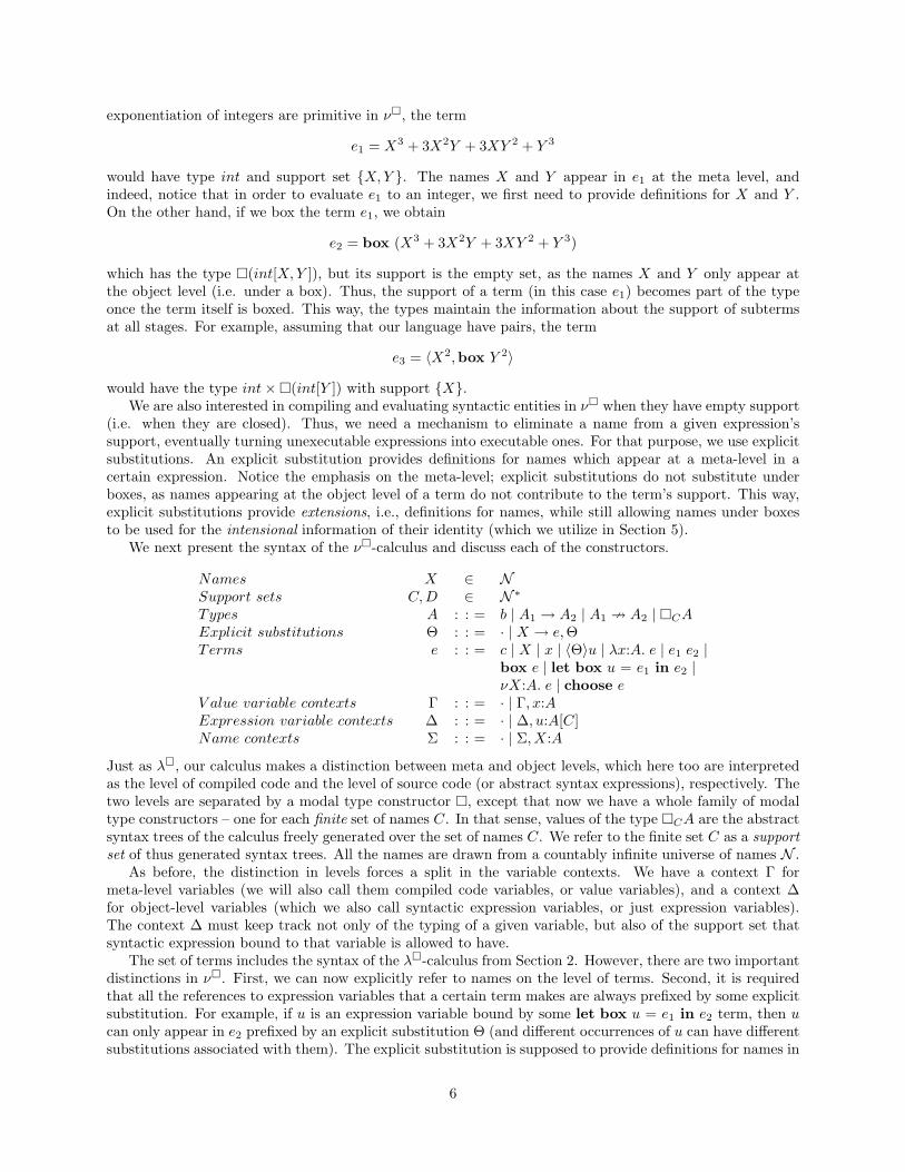
We next present the syntax of the ν�-calculus and discuss each of the constructors.

Names X ∈ NSupport sets C,D ∈ N ∗Types A : : = b | A1 → A2 | A1 9 A2 | �CAExplicit substitutions Θ : : = · | X → e,ΘTerms e : : = c | X | x | 〈Θ〉u | λx:A. e | e1 e2 |

box e | let box u = e1 in e2 |νX:A. e | choose e

V alue variable contexts Γ : : = · | Γ, x:AExpression variable contexts ∆ : : = · | ∆, u:A[C]Name contexts Σ : : = · | Σ, X:A

Just as λ�, our calculus makes a distinction between meta and object levels, which here too are interpretedas the level of compiled code and the level of source code (or abstract syntax expressions), respectively. Thetwo levels are separated by a modal type constructor �, except that now we have a whole family of modaltype constructors – one for each finite set of names C. In that sense, values of the type �CA are the abstractsyntax trees of the calculus freely generated over the set of names C. We refer to the finite set C as a supportset of thus generated syntax trees. All the names are drawn from a countably infinite universe of names N .

As before, the distinction in levels forces a split in the variable contexts. We have a context Γ formeta-level variables (we will also call them compiled code variables, or value variables), and a context ∆for object-level variables (which we also call syntactic expression variables, or just expression variables).The context ∆ must keep track not only of the typing of a given variable, but also of the support set thatsyntactic expression bound to that variable is allowed to have.

The set of terms includes the syntax of the λ�-calculus from Section 2. However, there are two importantdistinctions in ν�. First, we can now explicitly refer to names on the level of terms. Second, it is requiredthat all the references to expression variables that a certain term makes are always prefixed by some explicitsubstitution. For example, if u is an expression variable bound by some let box u = e1 in e2 term, then ucan only appear in e2 prefixed by an explicit substitution Θ (and different occurrences of u can have differentsubstitutions associated with them). The explicit substitution is supposed to provide definitions for names in

6

the expression bound to u. When the reference to the variable u is prefixed by an empty substitution, insteadof 〈·〉u we will simply write u. The explicit substitutions used in ν�-calculus are simultaneous substitutions.We assume that the syntactic presentation of a substitution never defines a denotation for the same nametwice.

Example 1 Assuming that X and Y are names of type int, the code segment below creates a polynomialover X and Y and then evaluates it at the point (X = 1, Y = 2).

- let box u = box (X3 + 3X2Y + 3XY2 + Y3)in

〈X -> 1, Y -> 2〉 uend

val it = 27 : int

�

The terms νx:A. e and choose e are the introduction and elimination form for the type constructorA 9 B. The term νX:A. e binds a name X of type A that can subsequently be used in e. The termchoose picks a fresh name of type A, substitutes it for the name bound in the argument ν-abstraction oftype A9 B, and proceeds to evaluate the body of the abstraction. To prevent the bound name in νX:A. efrom escaping the scope of its definition and thus creating an observable effect, the type system will enforcea discipline on the occurrence of X in e; X can appear in e only in the scope of some explicit substitutionwhich provides it with a definition, or in computationally irrelevant (i.e. dead code) positions.

Finally, enlarging an appropriate context by a new variable or a name is subject to Barendregt’s VariableConvention: the new variables and names are assumed distinct, or are renamed in order not to clash withalready existing ones. Terms which differ only in the syntactic representation of their bound variablesand names are considered equal. The binding forms in the language are λx:A. e, let box u = e1 in e2

and νX:A. e. As usual, capture-avoiding substitution [e1/x]e2 of expression e1 for the variable x in theexpression e2 is defined to rename bound variables and names when descending into their scope. Given aterm e, we denote by fv(e) and fn(e) the set of free variables of e and the set of names appearing in e at themeta-level. In addition, we overload the function fn so that given a type A and a support set C, fn(A[C])is the set of names appearing in A or C.

Example 2 To illustrate our new constructors, we present a version of the staged exponentiation functionthat we can write in ν�-calculus. In this and in other examples we resort to concrete syntax in ML fashion,and assume the presence of the base type of integers, recursive functions and let-definitions. In any case,these additions do not impose any theoretical difficulties.

fun exp (n : int) : �(int -> int) =choose (νX : int.

let fun exp’ (m : int) : �Xint =if m = 0 then box 1else

let box u = exp’ (m - 1)in

box (X * u)end

inlet box v = exp’ (n)in

box (λx:int. 〈X -> x〉 v)end

end)

7

- sq = exp 2;val sq = box (λx:int. x * (x * 1)) : �(int->int)

The function exp takes an integer n and generates a fresh name X of integer type. Then it calls the helperfunction exp’ to build the expression v = X ∗ · · · ∗X︸ ︷︷ ︸

n

∗1 of type int and support {X}. Finally, it turns

the expression v into a function by explicitly substituting the name X in v with a newly introduced boundvariable x. Notice that the generated residual code for sq does not contain any unnecessary redexes, incontrast to the λ� version of the program from Section 2. �

3.2 Explicit substitutions

In this section we formally introduce the concept of explicit substitution over names and define related oper-ations. As already outlined before, substitutions will serve to provide definitions for names, thus effectivelyremoving the substituting names from the support of the term in which they appear. Once the term hasempty support, it can be compiled and evaluated.

Definition 1 (Explicit substitution, its domain and range)An explicit substitution is a function from the set of names to the set of terms

Θ : N → Terms

Given a substitution Θ, its domain dom(Θ) is the set of names that the substitution does not fix. In otherwords

dom(Θ) = {X ∈ N | Θ (X) 6= X}

Range of a substitution Θ is the image of dom(Θ) under Θ:

range(Θ) = {Θ (X) | X ∈ dom(Θ)}

For the purposes of this work, we only consider substitutions with finite domains. A substitution Θ witha finite domain has a finitary syntactical representation as a set of ordered pairs X → e, relating a nameX from dom(Θ), with its substituting expression e. The opposite also holds – any finite and functionalset of ordered pairs of names and expressions determines a unique substitution. We will frequently equatea substitution and its syntactic representation when it does not result in ambiguities. Just as customary,we denote by fv(Θ) the set of free variables in the terms from range(Θ). The set of names appearing inrange(Θ) is denoted by fn(Θ).

Each substitution can be uniquely extended to a function over arbitrary terms in the following way.

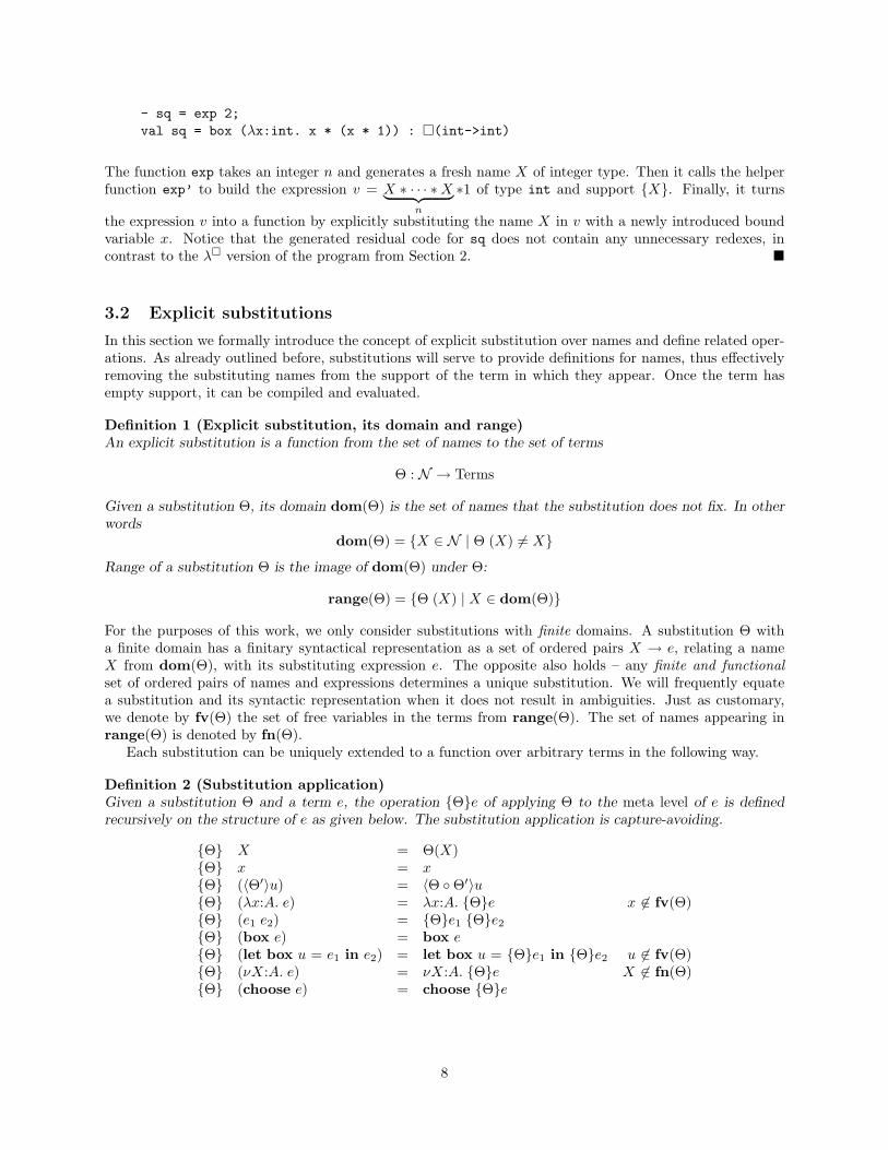
Definition 2 (Substitution application)Given a substitution Θ and a term e, the operation {Θ}e of applying Θ to the meta level of e is definedrecursively on the structure of e as given below. The substitution application is capture-avoiding.

{Θ} X = Θ(X){Θ} x = x{Θ} (〈Θ′〉u) = 〈Θ ◦Θ′〉u{Θ} (λx:A. e) = λx:A. {Θ}e x 6∈ fv(Θ){Θ} (e1 e2) = {Θ}e1 {Θ}e2

{Θ} (box e) = box e{Θ} (let box u = e1 in e2) = let box u = {Θ}e1 in {Θ}e2 u 6∈ fv(Θ){Θ} (νX:A. e) = νX:A. {Θ}e X 6∈ fn(Θ){Θ} (choose e) = choose {Θ}e

8

The most important aspect of the above definition is that substitution application does not recursivelydescend under box. This is of utmost importance for the soundness of our language as it preserves thedistinction between the meta and the object levels. It is also justified, as explicit substitutions are intendedto only remove names which are in the support of a term, and names appearing under box do not contributeto the support.

The operation of substitution application depends upon the operation of substitution composition Θ1◦Θ2,which we define next.

Definition 3 (Composition of substitutions)Given two substitutions Θ1 and Θ2 with finite domains, their composition Θ1 ◦Θ2 is the substitution definedas

(Θ1 ◦Θ2)(X) = {Θ1}(Θ2(X))

The composition of two substitutions with finite domains is well-defined, as the resulting mapping fromnames to terms is finite. Indeed, for every name X 6∈ dom(Θ1)∪dom(Θ2), we have that (Θ1 ◦Θ2)(X) = X,and therefore dom(Θ1 ◦Θ2) ⊆ dom(Θ1) ∪ dom(Θ2). Now, since this dom(Θ1 ◦Θ2) is finite, the syntacticrepresentation of the composition can easily be computed as the set

{X → {Θ1}(Θ2 (X)) | X ∈ dom(Θ1) ∪ dom(Θ2)}

It would occasionally be beneficial to represent this set as a disjoint union of two smaller sets Θ′1 and Θ′2defined as:

Θ′1 = {X → Θ1 (X) | X ∈ dom(Θ1) \ dom(Θ2)}Θ′2 = {X → {Θ1}(Θ2 (X)) | X ∈ dom(Θ2)}

It is important to notice that, though the definitions of substitution application and substitution com-position are mutually recursive, both the operations are terminating. Substitution application is definedinductively over the structure of its argument, so the size of terms on which it operates is always decreasing.Composing substitutions with finite domain also terminates. Indeed, as the above equations show, only afinite amount of work is needed to compute the domain of a composition. After the domain is obtained, thesyntactic representation of the composition is computed in finite time by substitution application.

3.3 Type system

The type system of our ν�-calculus consists of two mutually recursive judgments:

Σ; ∆; Γ ` e : A [C]

andΣ; ∆; Γ ` 〈Θ〉 : [C]⇒ [D]

Both of them are hypothetical and work with three contexts: context of names Σ, context of expressionvariables ∆, and a context of value variables Γ (the syntactic structure of all three contexts is given inSection 3.1). The first judgment is the typing judgment for expressions. Given an expression e it checkswhether e has type A, and is generated by the support set C. The second judgment types the explicitsubstitutions. Given a substitution Θ and two support sets C and D, the substitution has the type [C]⇒ [D]if it maps expressions of support C to expressions of support D. This intuition will be proved in Section 3.4.

The contexts deserve a few more words. Because the types of ν�-calculus depend on names, and types ofnames can depend on other names as well, we must impose some conditions on well-formedness of contexts.Henceforth, variable contexts ∆ and Γ will be well-formed relative to Σ if Σ declares all the names thatappear in the types of ∆ and Γ. A name context Σ is well-formed if every type in Σ uses only namesdeclared to the left of it. Further, we will often abuse the notation and write Σ = Σ′, X:A to define the setΣ′ obtained after removing the name X from the context Σ. Obviously, Σ′ does not have to be a well-formedcontext, as types in it may depend on X, but we will always transform Σ′ into a well-formed context before

9

Explicit substitutions

C ⊆ D

Σ; ∆; Γ ` 〈 〉 : [C]⇒ [D]

Σ; ∆; Γ ` e : A [D] Σ; ∆; Γ ` 〈Θ〉 : [C \ {X}]⇒ [D] X:A ∈ Σ

Σ; ∆; Γ ` 〈X → e,Θ〉 : [C]⇒ [D]

Hypothesis

X:A ∈ Σ

Σ; ∆; Γ ` X : A [X,C] Σ; ∆; (Γ, x:A) ` x : A [C]

Σ; (∆, u:A[C]); Γ ` 〈Θ〉 : [C]⇒ [D]

Σ; (∆, u:A[C]); Γ ` 〈Θ〉u : A [D]

λ-calculus

Σ; ∆; (Γ, x:A) ` e : B [C]

Σ; ∆; Γ ` λx:A. e : A→ B [C]

Σ; ∆; Γ ` e1 : A→ B [C] Σ; ∆; Γ ` e2 : A [C]

Σ; ∆; Γ ` e1 e2 : B [C]

Modality

Σ; ∆; · ` e : A [C]

Σ; ∆; Γ ` box e : �CA [D]

Σ; ∆; Γ ` e1 : �DA [C] Σ; (∆, u:A[D]); Γ ` e2 : B [C]

Σ; ∆; Γ ` let box u = e1 in e2 : B [C]

Names

(Σ, X:A); ∆; Γ ` e : B [C] X 6∈ fn(B[C])

Σ; ∆; Γ ` νX:A. e : A9 B [C]

Σ; ∆; Γ ` e : A9 B [C]

Σ; ∆; Γ ` choose e : B [C]

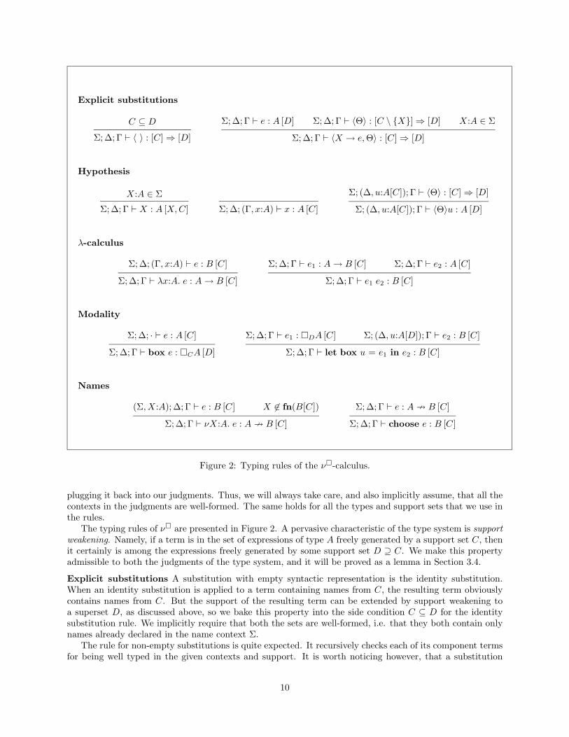
Figure 2: Typing rules of the ν�-calculus.

plugging it back into our judgments. Thus, we will always take care, and also implicitly assume, that all thecontexts in the judgments are well-formed. The same holds for all the types and support sets that we use inthe rules.

The typing rules of ν� are presented in Figure 2. A pervasive characteristic of the type system is supportweakening. Namely, if a term is in the set of expressions of type A freely generated by a support set C, thenit certainly is among the expressions freely generated by some support set D ⊇ C. We make this propertyadmissible to both the judgments of the type system, and it will be proved as a lemma in Section 3.4.

Explicit substitutions A substitution with empty syntactic representation is the identity substitution.When an identity substitution is applied to a term containing names from C, the resulting term obviouslycontains names from C. But the support of the resulting term can be extended by support weakening toa superset D, as discussed above, so we bake this property into the side condition C ⊆ D for the identitysubstitution rule. We implicitly require that both the sets are well-formed, i.e. that they both contain onlynames already declared in the name context Σ.

The rule for non-empty substitutions is quite expected. It recursively checks each of its component termsfor being well typed in the given contexts and support. It is worth noticing however, that a substitution

10

Θ can be given a type [C] ⇒ [D] where the “domain” support set C is completely unrelated to the setdom(Θ). In other words, the substitution can provide definitions for more names or for less names thanthe typing judgment actually cares for. For example, the substitution Θ = (X → 10, Y → 20) has domaindom(Θ) = {X,Y }, but it can be given (among others) the typings: [ ] ⇒ [ ], [X] ⇒ [ ], as well as[X,Y, Z]⇒ [Z].

Hypothesis rules Since there are three kinds of variable contexts, we have three hypothesis rules. Firstis the rule for names. A name X can be used provided it has been declared in Σ and is accounted forin the supplied support set. The implicit assumption is that the support set C is well-formed, i.e. thatC ⊆ dom (Σ) The rule for value variables is straightforward. The typing x:A can be inferred, if x:A isdeclared in Γ. The actual support of such a term can be any support set C as long as it is well-formed, whichis implicitly assumed. Expression variables occur in a term always prefixed with an explicit substitution.The rule for expression variables has to check if the expression variable is declared in the context ∆ and ifits corresponding substitution has the appropriate type.

λ-calculus fragment The rule for λ-abstraction is quite standard. Its implicit assumption is that theargument type A is well-formed in name context Σ before it is introduced into the variable context Γ.Application rule checks both the function and the application argument against the same support set.

Modal fragment Just as in λ�-calculus, the meaning of the rule for �-introduction is to ensure that theboxed expression e represents an abstract syntax tree. It checks e for having a given type in a context withoutcompile code variables. The support that e has to match is supplied as an index to the 2 constructor. Onthe other hand, the support for the whole expression box e is empty, as the expression obviously does notcontain any names at the meta level. Thus, the support can be arbitrarily weakened to any well-formedsupport set D. The �-elimination rule is also a straightforward extension of the corresponding λ� rule. Theonly difference is that the bound expression variable u from the context ∆ now has to be stored with itssupport annotation.

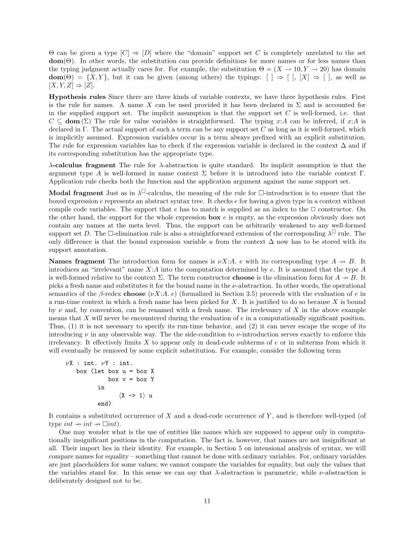
Names fragment The introduction form for names is νX:A. e with its corresponding type A 9 B. Itintroduces an “irrelevant” name X:A into the computation determined by e. It is assumed that the type Ais well-formed relative to the context Σ. The term constructor choose is the elimination form for A9 B. Itpicks a fresh name and substitutes it for the bound name in the ν-abstraction. In other words, the operationalsemantics of the β-redex choose (νX:A. e) (formalized in Section 3.5) proceeds with the evaluation of e ina run-time context in which a fresh name has been picked for X. It is justified to do so because X is boundby ν and, by convention, can be renamed with a fresh name. The irrelevancy of X in the above examplemeans that X will never be encountered during the evaluation of e in a computationally significant position.Thus, (1) it is not necessary to specify its run-time behavior, and (2) it can never escape the scope of itsintroducing ν in any observable way. The the side-condition to ν-introduction serves exactly to enforce thisirrelevancy. It effectively limits X to appear only in dead-code subterms of e or in subterms from which itwill eventually be removed by some explicit substitution. For example, consider the following term

νX : int. νY : int.box (let box u = box X

box v = box Yin

〈X -> 1〉 uend)

It contains a substituted occurrence of X and a dead-code occurrence of Y , and is therefore well-typed (oftype int9 int9 �int).

One may wonder what is the use of entities like names which are supposed to appear only in computa-tionally insignificant positions in the computation. The fact is, however, that names are not insignificant atall. Their import lies in their identity. For example, in Section 5 on intensional analysis of syntax, we willcompare names for equality – something that cannot be done with ordinary variables. For, ordinary variablesare just placeholders for some values; we cannot compare the variables for equality, but only the values thatthe variables stand for. In this sense we can say that λ-abstraction is parametric, while ν-abstraction isdeliberately designed not to be.

11

It is only that names appear irrelevant because we have to force a certain discipline upon their usage.In particular, before leaving the local scope of some name X, as determined by its introducing ν, we haveto “close up” the resulting expression if it depends significantly on X. This “closure” can be achieved byturning the expression into a λ-abstraction by means of explicit substitutions. Otherwise, the introductionof the new name will be an observable effect. To paraphrase, when leaving the scope of X, we have to turnthe “polynomials” depending on X into functions. An illustration of this technique is the program alreadypresented in Example 2.

The previous version of this work [Nan02] did not use the constructors ν and choose, but rather combinedthem into a single constructor new. This is also the case in the work of Pitts and Gabbay [PG00]. Thedecomposition is given by the equation

new X:A in e = choose (νX:A. e)

We have decided on this reformulation in order to make the types of the language follow more closely theintended meaning of the terms and thus provide a stronger logical foundation for the calculus.

3.4 Structural properties

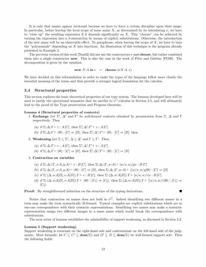
This section explores the basic theoretical properties of our type system. The lemmas developed here will beused to justify the operational semantics that we ascribe to ν�-calculus in Section 3.5, and will ultimatelylead to the proof of the Type preservation and Progress theorems.

Lemma 4 (Structural properties of contexts)1. Exchange Let Σ′, ∆′ and Γ′ be well-formed contexts obtained by permutation from Σ, ∆ and Γ

respectively. Then

(a) if Σ; ∆; Γ ` e : A [C], then Σ′; ∆′; Γ′ ` e : A [C]

(b) if Σ; ∆; Γ ` 〈Θ〉 : [C]⇒ [D], then Σ′; ∆′; Γ′ ` 〈Θ〉 : [C]⇒ [D], then

2. Weakening Let Σ ⊆ Σ′, ∆ ⊆ ∆′ and Γ ⊆ Γ′. Then

(a) if Σ; ∆; Γ ` e : A [C], then Σ′; ∆′; Γ′ ` e : A [C]

(b) if Σ; ∆; Γ ` 〈Θ〉 : [C]⇒ [D], then Σ′; ∆′; Γ′ ` 〈Θ〉 : [C]⇒ [D]

3. Contraction on variables

(a) if Σ; ∆; (Γ, x:A, y:A) ` e : B [C], then Σ; ∆; (Γ, w:A) ` [w/x,w/y]e : B [C]

(b) if Σ; ∆; (Γ, x:A, y:A) ` 〈Θ〉 : [C]⇒ [D], then Σ; ∆; (Γ, w:A) ` 〈[w/x,w/y]Θ〉 : [C]⇒ [D]

(c) if Σ; (∆, u:A[D], v:A[D]); Γ ` e : B [C], then Σ; (∆, w:A[D]); Γ ` [w/u,w/v]e : B [C].

(d) if Σ; (∆, u:A[D], v:A[D]); Γ ` 〈Θ〉 : [C1] ⇒ [C2], then Σ; (∆, w:A[D]); Γ ` 〈[w/u,w/v]Θ〉 : [C1] ⇒[C2].

Proof: By straightforward induction on the structure of the typing derivations. �

Notice that contraction on names does not hold in ν�. Indeed identifying two different names in aterm may make the term syntactically ill-formed. Typical examples are explicit substitutions which are inone-one correspondence with their syntactic representations. Identifying two names may make a syntacticrepresentation assign two different images to a same name which would break the correspondence withsubstitutions.

The next series of lemmas establishes the admissibility of support weakening, as discussed in Section 3.3.

Lemma 5 (Support weakening)Support weakening is covariant on the right-hand side and contravariant on the left-hand side of the judg-ments. More formally, let C ⊆ C ′ ⊆ dom(Σ) and D′ ⊆ D ⊆ dom(Σ) be well-formed support sets. Thenthe following holds:

12

1. if Σ; ∆; Γ ` e : A [C], then Σ; ∆; Γ ` e : A [C ′].

2. if Σ; ∆; Γ ` 〈Θ〉 : [D]⇒ [C], then Σ; ∆; Γ ` 〈Θ〉 : [D]⇒ [C ′].

3. if Σ; (∆, u:A[D]); Γ ` e : B [C], then Σ; (∆, u:A[D′]); Γ ` e : B [C]

4. if Σ; ∆; Γ ` 〈Θ〉 : [D]⇒ [C], then Σ; ∆; Γ ` 〈Θ〉 : [D′]⇒ [C].

Proof: The first two statements are proved by straightforward simultaneous induction on the given deriva-tions. The third and the fourth part are proved by induction on the structure of their respective derivations.

�

Lemma 6 (Support extension)Let D ⊆ dom(Σ) be a well-formed support set. Then the following holds:

1. if Σ; (∆, u:A[C1]); Γ ` e : B [C2] then Σ; (∆, u:A[C1 ∪D]); Γ ` e : B [C2 ∪D]

2. if Σ; ∆; Γ ` 〈Θ〉 : [C1]⇒ [C2], then Σ; ∆; Γ ` 〈Θ〉 : [C1 ∪D]⇒ [C2 ∪D]

Proof: By induction on the structure of the derivations. �

Lemma 7 (Substitution merge)If Σ; ∆; Γ ` 〈Θ〉 : [C1] ⇒ [D] and Σ; ∆; Γ ` 〈Θ′〉 : [C2] ⇒ [D] where dom(Θ) ∩ dom(Θ′) = ∅, then〈Θ,Θ′〉 : [C1 ∪ C2]⇒ [D].

Proof: By induction on the structure of Θ′. �

The following lemma shows that the intuition behind the typing judgment for explicit substitution ex-plained in Section 3.3 is indeed valid.

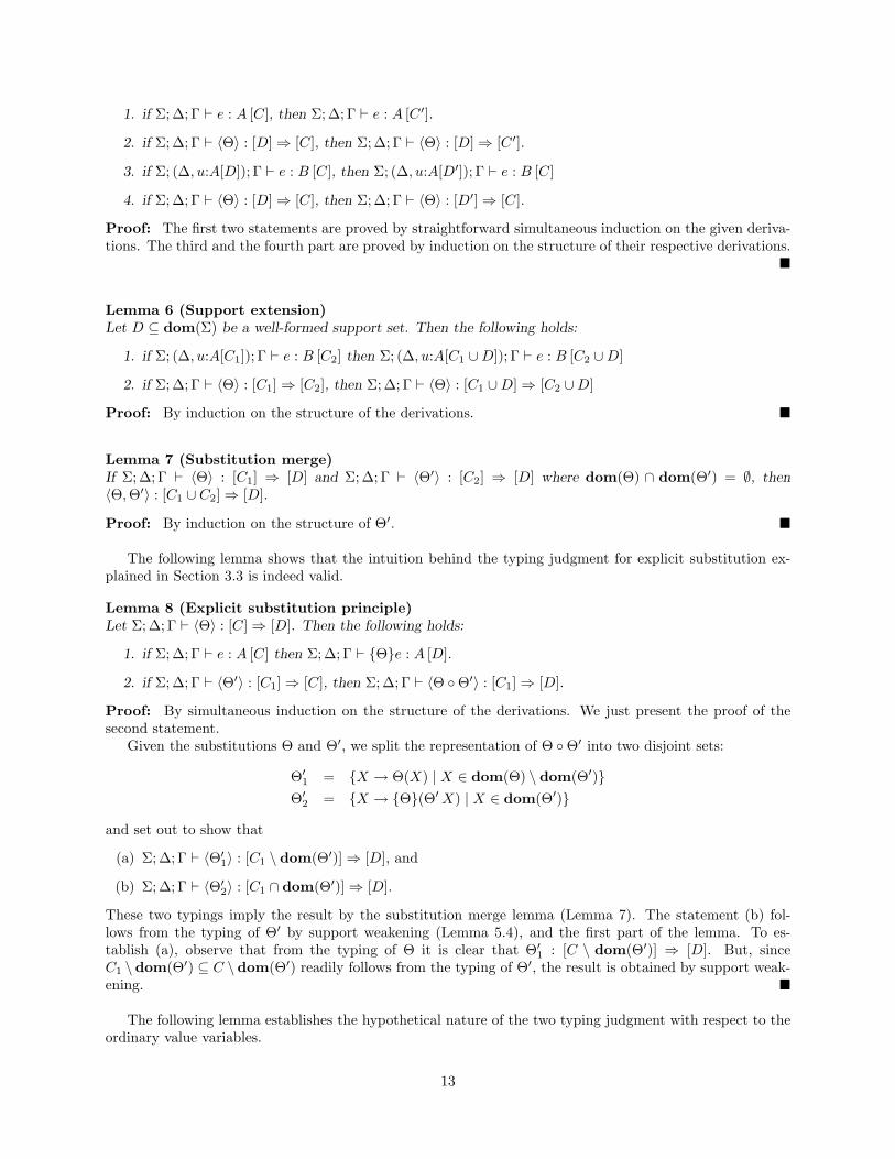
Lemma 8 (Explicit substitution principle)Let Σ; ∆; Γ ` 〈Θ〉 : [C]⇒ [D]. Then the following holds:

1. if Σ; ∆; Γ ` e : A [C] then Σ; ∆; Γ ` {Θ}e : A [D].

2. if Σ; ∆; Γ ` 〈Θ′〉 : [C1]⇒ [C], then Σ; ∆; Γ ` 〈Θ ◦Θ′〉 : [C1]⇒ [D].

Proof: By simultaneous induction on the structure of the derivations. We just present the proof of thesecond statement.

Given the substitutions Θ and Θ′, we split the representation of Θ ◦Θ′ into two disjoint sets:

Θ′1 = {X → Θ(X) | X ∈ dom(Θ) \ dom(Θ′)}Θ′2 = {X → {Θ}(Θ′X) | X ∈ dom(Θ′)}

and set out to show that

(a) Σ; ∆; Γ ` 〈Θ′1〉 : [C1 \ dom(Θ′)]⇒ [D], and

(b) Σ; ∆; Γ ` 〈Θ′2〉 : [C1 ∩ dom(Θ′)]⇒ [D].

These two typings imply the result by the substitution merge lemma (Lemma 7). The statement (b) fol-lows from the typing of Θ′ by support weakening (Lemma 5.4), and the first part of the lemma. To es-tablish (a), observe that from the typing of Θ it is clear that Θ′1 : [C \ dom(Θ′)] ⇒ [D]. But, sinceC1 \dom(Θ′) ⊆ C \dom(Θ′) readily follows from the typing of Θ′, the result is obtained by support weak-ening. �

The following lemma establishes the hypothetical nature of the two typing judgment with respect to theordinary value variables.

13

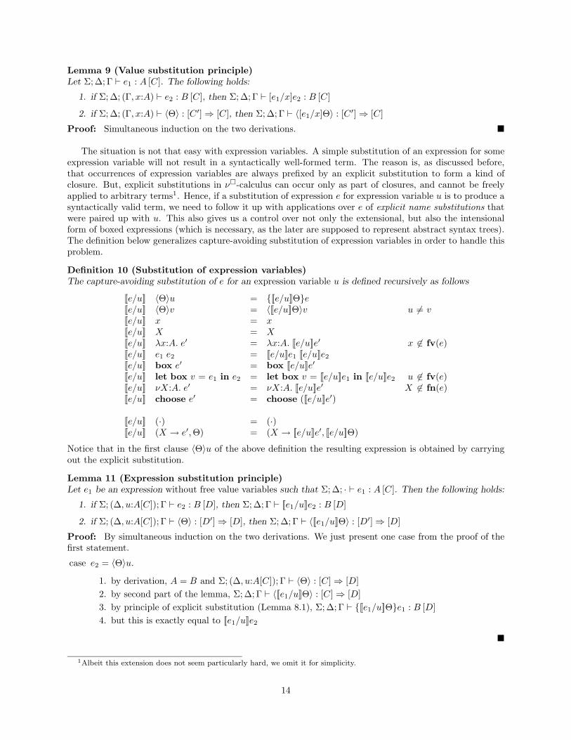
Lemma 9 (Value substitution principle)Let Σ; ∆; Γ ` e1 : A [C]. The following holds:

1. if Σ; ∆; (Γ, x:A) ` e2 : B [C], then Σ; ∆; Γ ` [e1/x]e2 : B [C]

2. if Σ; ∆; (Γ, x:A) ` 〈Θ〉 : [C ′]⇒ [C], then Σ; ∆; Γ ` 〈[e1/x]Θ〉 : [C ′]⇒ [C]

Proof: Simultaneous induction on the two derivations. �

The situation is not that easy with expression variables. A simple substitution of an expression for someexpression variable will not result in a syntactically well-formed term. The reason is, as discussed before,that occurrences of expression variables are always prefixed by an explicit substitution to form a kind ofclosure. But, explicit substitutions in ν�-calculus can occur only as part of closures, and cannot be freelyapplied to arbitrary terms1. Hence, if a substitution of expression e for expression variable u is to produce asyntactically valid term, we need to follow it up with applications over e of explicit name substitutions thatwere paired up with u. This also gives us a control over not only the extensional, but also the intensionalform of boxed expressions (which is necessary, as the later are supposed to represent abstract syntax trees).The definition below generalizes capture-avoiding substitution of expression variables in order to handle thisproblem.

Definition 10 (Substitution of expression variables)The capture-avoiding substitution of e for an expression variable u is defined recursively as follows

[[e/u]] 〈Θ〉u = {[[e/u]]Θ}e[[e/u]] 〈Θ〉v = 〈[[e/u]]Θ〉v u 6= v[[e/u]] x = x[[e/u]] X = X[[e/u]] λx:A. e′ = λx:A. [[e/u]]e′ x 6∈ fv(e)[[e/u]] e1 e2 = [[e/u]]e1 [[e/u]]e2

[[e/u]] box e′ = box [[e/u]]e′

[[e/u]] let box v = e1 in e2 = let box v = [[e/u]]e1 in [[e/u]]e2 u 6∈ fv(e)[[e/u]] νX:A. e′ = νX:A. [[e/u]]e′ X 6∈ fn(e)[[e/u]] choose e′ = choose ([[e/u]]e′)

[[e/u]] (·) = (·)[[e/u]] (X → e′,Θ) = (X → [[e/u]]e′, [[e/u]]Θ)

Notice that in the first clause 〈Θ〉u of the above definition the resulting expression is obtained by carryingout the explicit substitution.

Lemma 11 (Expression substitution principle)Let e1 be an expression without free value variables such that Σ; ∆; · ` e1 : A [C]. Then the following holds:

1. if Σ; (∆, u:A[C]); Γ ` e2 : B [D], then Σ; ∆; Γ ` [[e1/u]]e2 : B [D]

2. if Σ; (∆, u:A[C]); Γ ` 〈Θ〉 : [D′]⇒ [D], then Σ; ∆; Γ ` 〈[[e1/u]]Θ〉 : [D′]⇒ [D]

Proof: By simultaneous induction on the two derivations. We just present one case from the proof of thefirst statement.

case e2 = 〈Θ〉u.

1. by derivation, A = B and Σ; (∆, u:A[C]); Γ ` 〈Θ〉 : [C]⇒ [D]2. by second part of the lemma, Σ; ∆; Γ ` 〈[[e1/u]]Θ〉 : [C]⇒ [D]3. by principle of explicit substitution (Lemma 8.1), Σ; ∆; Γ ` {[[e1/u]]Θ}e1 : B [D]4. but this is exactly equal to [[e1/u]]e2

�

1Albeit this extension does not seem particularly hard, we omit it for simplicity.

14

Σ, e1 7−→ Σ′, e′1

Σ, (e1 e2) 7−→ Σ′, (e′1 e2)

Σ, e2 7−→ Σ′, e′2

Σ, (v1 e2) 7−→ Σ′, (v1 e′2) Σ, (λx:A. e) v 7−→ Σ, [v/x]e

Σ, e1 7−→ Σ′, e′1

Σ, (let box u = e1 in e2) 7−→ Σ′, (let box u = e′1 in e2)

Σ, (let box u = box e1 in e2) 7−→ Σ, [[e1/u]]e2

Σ, e 7−→ Σ′, e′

Σ, choose e 7−→ Σ′, choose e′ Σ, choose (νX:A. e) 7−→ (Σ, X:A), e

Figure 3: Structured operational semantics of ν�-calculus.

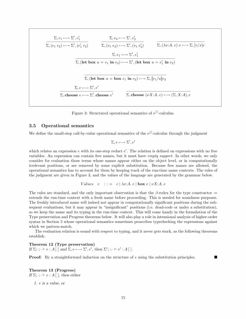
3.5 Operational semantics

We define the small-step call-by-value operational semantics of the ν�-calculus through the judgment

Σ, e 7−→ Σ′, e′

which relates an expression e with its one-step reduct e′. The relation is defined on expressions with no freevariables. An expression can contain free names, but it must have empty support. In other words, we onlyconsider for evaluation those terms whose names appear either on the object level, or in computationallyirrelevant positions, or are removed by some explicit substitution. Because free names are allowed, theoperational semantics has to account for them by keeping track of the run-time name contexts. The rules ofthe judgment are given in Figure 3, and the values of the language are generated by the grammar below.

V alues v : : = c | λx:A. e | box e | νX:A. e

The rules are standard, and the only important observation is that the β-redex for the type constructor 9extends the run-time context with a fresh name before proceeding. This is needed for soundness purposes.The freshly introduced name will indeed not appear in computationally significant positions during the sub-sequent evaluations, but it may appear in “insignificant” positions (i.e. dead-code or under a substitution),so we keep the name and its typing in the run-time context. This will come handy in the formulation of theType preservation and Progress theorems below. It will also play a role in intensional analysis of higher-ordersyntax in Section 5 whose operational semantics sometimes proscribes typechecking the expressions againstwhich we pattern-match.

The evaluation relation is sound with respect to typing, and it never gets stuck, as the following theoremsestablish.

Theorem 12 (Type preservation)If Σ; ·; · ` e : A [ ] and Σ, e 7−→ Σ′, e′, then Σ′; ·; · ` e′ : A [ ].

Proof: By a straightforward induction on the structure of e using the substitution principles. �

Theorem 13 (Progress)If Σ; ·; · ` e : A [ ], then either

1. e is a value, or

15

2. there exist a term e′ and a context Σ′ extending Σ, such that Σ, e 7−→ Σ′, e′.

Proof: By a straightforward induction on the structure of e. �

The progress theorem seems to indicate that the evaluation relation is not deterministic, as each termmay have more then one reduct. However, all these reducts are different only in the identity of the newlyintroduced irrelevant names, as the lemma below establishes.

Lemma 14 (Determinacy)If Σ; ·; · ` e : A [ ] and Σ, e 7−→ Σ1, e1 and Σ, e 7−→ Σ2, e2, then there exists a permutation of namesπ : N → N , fixing dom(Σ), such that Σ1 = π(Σ2) and e1 = π(e2).

Proof: By induction on the structure of e. The only interesting case is when e = choose (νX:A. e′). Thenit must be e1 = [X1/X]e′, e2 = [X2/X]e′, and Σ1 = (Σ, X1:A), Σ2 = (Σ, X2:A), where X1, X2 ∈ N arefresh. Obviously, the involution π = (X1 X2) which swaps these two names has the required properties. �

4 Support polymorphism

It is frequently necessary to write programs which are polymorphic in the support of their syntactic object-level arguments, because they are intended to manipulate abstract syntax trees whose support is not knownat compile time. A typical example would be a function which recurses over some syntax tree with bindingstructure When it encounters a λ-abstraction, it has to place a fresh name instead of the bound variable,and recursively continue scanning the body of the λ-abstraction, which is itself a syntactic expression butdepending on this newly introduced name.2 For such uses, we extend the ν�-calculus with a notion ofexplicit support polymorphism in the style of Girard and Reynolds [Gir86, Rey83]. It turns out that theconstructs explained here will also play a role in intensional analysis of higher-order syntax in Section 5 as arepresentation mechanism for encoding object-level functions as meta functions over object-level expressions.

The addition of support polymorphism to the simple ν�-calculus starts with syntactic changes that wesummarize below.

Support variables p, q ∈ PSupport sets C,D ∈ (N ∪ P)∗

Types A : : = . . . | ∀p. ATerms e : : = . . . | Λp. e | e [C]Name context Σ : : = . . . | Σ, pV alues v : : = . . . | Λp. e

We introduce a new syntactic category of support variables, which are intended to stand for unknown supportsets. In addition, the support sets themselves are now allowed to contain these support variables, to expressthe situation in which only a portion of a support set is unknown. Consequently, the function fn(−) mustbe updated to now return the set of names and support variables appearing in its argument. The languageof types is extended with the type ∀p. A expressing universal support quantification. Its introduction formis Λp. e, which abstracts an unknown support set p in the expression e. This Λ-abstraction will also be avalue in the extended operational semantics. The corresponding elimination form is the application e [C]whose meaning is to instantiate the unknown support set abstracted in e with the provided support set C.Because now the types can depend on names as well as on support variables, the name contexts must declareboth. We assume the same convention on well-formedness of the name context as before.

The typing judgment has to be instrumented with new rules for typing support-polymorphic abstractionand application.

(Σ, p); ∆; Γ ` e : A [C] p 6∈ C

Σ; ∆; Γ ` Λp. e : ∀p. A [C]

Σ; ∆; Γ ` e : ∀p. A [C]

Σ; ∆; Γ ` e [D] : ([D/p]A) [C]

2The calculus described here cannot support this scenario yet because it lacks type polymorphism and type-polymorphicrecursion, but support polymorphism is a necessary step in that direction.

16

The ∀-introduction rule requires that the bound variable p does not escape the scope of the constructors ∀and Λ which bind it. In particular it must be p 6∈ C. The convention also assumes implicitly that p 6∈ Σ,before it can be added. The rule for ∀-elimination substitutes the argument support set D into the typeA. It assumes that D is well-formed relative to the context Σ, i.e. that D ⊆ dom(Σ). The operationalsemantics for the new constructs is also not surprising.

Σ, e 7−→ Σ′, e′

Σ, (e [C]) 7−→ Σ′, (e′ [C]) Σ, (Λp. e) [C] 7−→ Σ, [C/p]e

The extended language satisfies the following substitution principle.

Lemma 15 (Support substitution principle)Let Σ = (Σ1, p,Σ2) and D ⊆ dom(Σ1) and denote by (−)′ the operation of substituting D for p. Then thefollowing holds.

1. if Σ; ∆; Γ ` e : A [C], then (Σ1,Σ′2); ∆′; Γ′ ` e′ : A′ [C ′]

2. if Σ; ∆; Γ ` Θ : C1 → C2, then (Σ1,Σ′2); ∆′; Γ′ ` Θ′ : C ′1 → C ′2

Proof: By simultaneous induction on the two derivations. �

The structural properties presented in Section 3.4 readily extend to the new language with supportpolymorphism. We present the extended versions, as well as their proofs, in the Appendix. The same istrue of the Type preservation and Progress theorems (Theorem 12 and 13) whose additional cases involvingsupport abstraction and application are handled using the above Lemma 15.

Example 3 In a support-polymorphic ν�-calculus we can slightly generalize the program from Example 2by pulling out the helper function exp’ and parametrizing it over the exponentiating expression. In theconcrete syntax below we symbolize by [p] that p is a support variable abstracted in the function definition.

fun exp’ [p] (e : �pint) (n : int) : �pint =if n = 0 then box 1else

let box u = exp’ [p] e (n - 1)box w = e

inbox (u * w)

end

fun exp (n : int) : �(int -> int) =choose (νX : int.

let box w = exp’ [X] (box X) nin

box (λx:int. 〈X -> x〉 w)end)

- sq = exp 2;val sq = box (λx:int. x * (x * 1)) : �(int->int)

�

In the development of the ν�-calculus we have had a particular semantic interpretation in mind of objectlevel expressions as abstract syntax trees representing templates for source programs. This interpretationwill be exploited in an essential way in Section 5. Notice, however, that the fragment presented thus far isnot necessarily committed to viewing the object expressions as syntax. It is quite possible (and it remainsan important future work) that boxed expressions of core ν� with support polymorphism can be storedin run-time in some intermediate or even compiled form, which might be beneficial to the efficiency of thecalculus.

17

5 Intensional analysis of higher-order syntax

5.1 Syntax and typechecking

As explained in Section 3, we interpret the type �CA as a set of syntactic expressions of type A freelygenerated over the set of “indeterminates” C. The calculus presented so far was capable of constructingvalues of type �CA, but it is obviously desirable to provide capabilities for inspecting and destructing thesesyntax trees. Here we extend the support-polymorphic ν�-calculus with primitives for pattern-matchingagainst syntactic expressions with binding structure. For reasons of simplicity, we develop the extension inthe setup of our calculus, where the languages used in the meta and the object levels are the same. But thisis not necessary, as the same mechanism would work for any object level calculus with binding structure.As a matter of fact, it is probably more appropriate to emphasize the distinction between meta and objectcalculi, because even the pattern-matching presented here can recognize only a subset of term constructors ofν�. In particular, we can only test if an expression is a name, or a λ-abstraction or an application. It is notclear whether the expressiveness of pattern-matching can be extended to handle a larger subset of the object-language without significant additions to the meta-language. But this would in turn require extensions topattern-match against the additions, which would in turn require new extensions to the meta-language, andso on.

The syntactic additions that we consider in this section are summarized in the the table below.

Pattern variables w ∈ WHigher-order patterns π : : = (w x1 . . . xn):A[C] | X | x | λx:A. π | π1 π2

Pattern assignments σ : : = · | w → e, σTerms e : : = . . . | case e of box π ⇒ e1 else e2

We use higher-order patterns [Mil90] to match against syntactic expressions with binding structure. Higher-order patterns introduce two unrelated notions of variables that we must distinguish between. First is theconcept of free variables. These are introduced by patterns for binding structure λx:A. π and are syntacticentities that can match only themselves. Second is the concept of pattern variables. They are placeholdersintended to bind syntactic subexpressions in the process of matching and pass them to the subsequentcomputation. We use x, y and variants to range over bound variables, and w and variants to range overpattern variables.

The basic pattern (w x1 . . . xn):A[C] declares a pattern variable w which will be allowed to match asyntactic expression of type A and support C subject to the condition that the expression’s free variables areamong x1, . . . , xn. Pattern X matches a name X from the global name context. Pattern λx:A. π matches aλ-abstraction of domain type A. It declares a new free variable x which is local to the pattern, and demandsthat the body of the matched expression conforms to the pattern π. A free variable x matches only thepattern x. Pattern π1 π2 matches a syntactic expression representing application. Notice that the decisionto explicitly assign types to every pattern variable forces the pattern for application to be monomorphic.In other words, the application pattern cannot match a pair of expressions representing a function and itsargument if the domain type of the function is now known in advance. It is an important future work toextend intensional analysis to allow patterns which are type-polymorphic in this sense. The patterns areassumed to be linear, i.e. no pattern variable occurs twice.

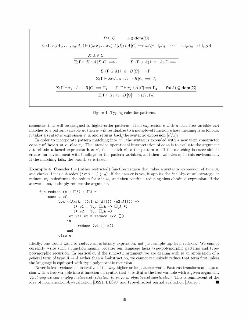
The typing judgment for patterns has the form

Σ; Γ ` π : A [C] =⇒ Γ1

It is hypothetical in the global context of names Σ, and the context of locally declared free variables Γ. Itchecks whether the pattern π has type A and support C and if the pattern variables from π conform tothe typings given in the residual context Γ1. The typing rules are presented in Figure 4. Most of them arestraightforward and we do not explain them, but the rule for pattern variables deserves special attention.As it shows, in order for the pattern expression (w x1 . . . xn):A[C] to be well-typed, the free variablesx1:A1, . . . , xn:An have to be declared in the local context Γ and the support set D ⊆ C. Then w will matchonly expressions of type A with the given free variables and the names declared in D. The residual contexttypes w as a meta-level function over types �pAi with polymorphic support. This hints at the operational

18

D ⊆ C p 6∈ dom(Σ)

Σ; (Γ, x1:A1, . . . , xn:An) ` ((w x1 . . . xn):A[D]) : A [C] =⇒ w:∀p. �pA1 → · · · → �pAn → �p,DA

X:A ∈ Σ

Σ; Γ ` X : A [X,C] =⇒ · Σ; (Γ, x:A) ` x : A [C] =⇒ ·

Σ; (Γ, x:A) ` π : B [C] =⇒ Γ1

Σ; Γ ` λx:A. π : A→ B [C] =⇒ Γ1

Σ; Γ ` π1 : A→ B [C] =⇒ Γ1 Σ; Γ ` π2 : A [C] =⇒ Γ2 fn(A) ⊆ dom(Σ)

Σ; Γ ` π1 π2 : B [C] =⇒ (Γ1,Γ2)

Figure 4: Typing rules for patterns.

semantics that will be assigned to higher-order patterns. If an expression e with a local free variable x:Amatches to a pattern variable w, then w will residualize to a meta-level function whose meaning is as follows:it takes a syntactic expression e′:A and returns back the syntactic expression [e′/x]e.

In order to incorporate pattern matching into ν�, the syntax is extended with a new term constructorcase e of box π ⇒ e1 else e2. The intended operational interpretation of case is to evaluate the argumente to obtain a boxed expression box e′, then match e′ to the pattern π. If the matching is successful, itcreates an environment with bindings for the pattern variables, and then evaluates e1 in this environment.If the matching fails, the branch e2 is taken.

Example 4 Consider the (rather restricted) function reduce that takes a syntactic expression of type A,and checks if it is a β-redex (λx:A. w1) (w2). If the answer is yes, it applies the “call-by-value” strategy: itreduces w2, substitutes the reduct for x in w1 and then continue reducing thus obtained expression. If theanswer is no, it simply returns the argument.

fun reduce (e : �A) : �A =case e of

box ((λx:A. ((w1 x):A[])) (w2:A[])) =>(* w1 : ∀q. �qA -> �qA *)(* w2 : ∀q. �qA *)

let val e2 = reduce (w2 [])in

reduce (w1 [] e2)end

else e

Ideally, one would want to reduce an arbitrary expression, not just simple top-level redexes. We cannotcurrently write such a function mainly because our language lacks type-polymorphic patterns and type-polymorphic recursion. In particular, if the syntactic argument we are dealing with is an application of ageneral term of type A→ A rather than a λ-abstraction, we cannot recursively reduce that term first unlessthe language is equipped with type-polymorphic recursion.

Nevertheless, reduce is illustrative of the way higher-order patterns work. Patterns transform an expres-sion with a free variable into a function on syntax that substitutes the free variable with a given argument.That way we can employ meta-level reduction to perform object-level substitution. This is reminiscent of theidea of normalization-by-evaluation [BS91, BES98] and type-directed partial evaluation [Dan96]. �

19

The typing rule for case is:

Σ; ∆; Γ ` e : �DA [C] Σ; · ` π : A [D] =⇒ Γ1 Σ; ∆; (Γ,Γ1) ` e1 : B [C] Σ; ∆; Γ ` e2 : B [C]

Σ; ∆; Γ ` case e of box π ⇒ e1 else e2 : B [C]

Observe that the second premise of the rule requires an empty variable context, so that patterns cannotcontain outside value or expression variables. However (and this is important), they can contain names. Itis easy to incorporate the new syntax into the language. We first extend explicit substitution over the newcase construct

{Θ} (case e of box π ⇒ e1 else e2) = case ({Θ}e) of box π ⇒ ({Θ}e1) else ({Θ}e2)

and similarly for expression substitution, and then all the structural properties derived in Section 3.4 easilyhold. The only complication comes in handling names and support substitution because patterns are allowedto depend on names and support variables from the global context Σ. However, the lemmas below establishthe required invariants.

Lemma 16 (Structural properties of pattern matching)1. Exchange Let Σ′, Γ′ and Γ′1 be well-formed contexts obtained by permutation from Σ, Γ and Γ1

respectively and Σ; Γ ` π : A [C] =⇒ Γ1. Then Σ′; Γ′ ` π : A [C] =⇒ Γ′1

2. Weakening Let Σ ⊆ Σ′ and Σ; Γ ` π : A [C] =⇒ Γ1. Then Σ′; Γ ` π : A [C] =⇒ Γ1

Proof: By straightforward introduction on the structure of the typing derivations. �

Lemma 17 (Support substitution principle for pattern matching)Let Σ = (Σ1, p,Σ2) and D ⊆ dom(Σ1) and denote by (−)′ the operation of substituting D for p. Assumealso that Σ; Γ ` π : A [C] =⇒ Γ1. Then (Σ1,Σ′2); Γ′ ` π′ : A′ [C ′] =⇒ Γ′1.

Proof: By straightforward induction on the structure of π. �

5.2 Operational semantics

Operational semantics for pattern matching is given through the new judgment

Σ; Γ ` e� π =⇒ σ

which reads: in a global context of names and support variables Σ and a context of locally declared freevariables Γ the matching of the expression e to the pattern π generates an assignment of values σ to thepattern variables of π. The rules for this judgment are given in Figure 5. Most of the rules are self-evident,but the rule for pattern variables deserves more attention. Its premise requires a run-time typecheck of theexpression e in the given contexts. That is why the operational semantics of ν�-calculus (see Section 3.5)must carry around at run-time the list of currently defined names and their typings. The following lemmarelates the typing judgment for patterns and their operational semantics.

Lemma 18 (Soundness of pattern matching)Let π be a pattern such that Σ; Γ ` π : A [C] =⇒ Γ1, where Γ1 = (w1:A1, . . . , wn:An). Furthermore, lete be an expression matching π to produce a pattern assignment σ, i.e. Σ; Γ ` e � π : A =⇒ σ. Thenσ = (w1 → e1, . . . , wn → en) where Σ; ·; · ` ei : A1, for every i = 1, . . . , n.

Notice that in the lemma we did not require that e be well-typed, or even syntactically well-formed. If itwere not well-formed, the matching simply would not succeed.

Proof: By induction on the structure of π. We present the base case below.

20

Σ; ·; (x1:A1, . . . , xn:An) ` e : A [D]

Σ; (Γ, x1:A1, . . . , xn:An) ` e� ((w x1 . . . xn):A[D]) : A =⇒ [w → Λp. λyi:�pAi. let box xi = yi in box e]

(Σ, X:A); Γ ` X �X : A =⇒ · Σ; (Γ, x:A) ` x� x : A =⇒ ·

Σ; (Γ, x:A) ` e� π : B =⇒ σ

Σ; Γ ` λx:A. e� λx:A. π : (A→ B) =⇒ σ

Σ; Γ ` e1 � π1 : A→ B =⇒ σ1 Σ; Γ ` e2 � π2 : A =⇒ σ2

Σ; Γ ` e1 e2 � π1 π2 : B =⇒ (σ1, σ2)

Figure 5: Operational semantics for pattern matching.

case π = (w x1 . . . xn):A[D], where Γ = Γ2, xi:Ai.

1. let e′ = (Λp. λyi:�pAi. let box xi = yi in box e) and A′ = ∀p. �pA1 → · · · → �pAn → �p,DA2. by typing derivation, D ⊆ C and xi:Ai ∈ Γ and also Γ1 = (w:A′)

3. by matching derivation, Σ; ·; (x1:A1, . . . , xn:An) ` e : A [D], and σ = (w → e′)

4. by straightforward structural induction, Σ; (x1:A1, . . . , xn:An); · ` e : A [D]

5. by support weakening, (Σ, p); (x1:A1[p], . . . , xn:An[p]); · ` e : A [D, p]

6. and thus also, (Σ, p); (x1:A1[p], . . . , xn:An[p]); · ` box e : �D,pA [ ]

7. and (Σ, p); ·; (y1:�pA1, . . . , yn:�pAn) ` let box xi = yi in box e : �D,pA [ ]

8. and finally, Σ; ·; · ` e′ : A′ [ ]

�The last piece to be added is the operational semantics for the case statement, and the required rules aregiven below. Notice that the premise of last rule makes use of the fact that the operational semantics forpatterns is deterministic; the rule applies if the expression and e and the pattern π cannot be matched.

Σ, e 7−→ Σ′, e′

Σ, (case e of box π ⇒ e1 else e2) 7−→ Σ′, (case e′ of box π ⇒ e1 else e2)

Σ; · ` e� π : A =⇒ (w1 → e′1, . . . , wn → e′n)

Σ, (case box e of box π ⇒ e1 else e2) 7−→ Σ, [e′1/w1, . . . , e′n/wn]e1

Σ; · ` e� π 6=⇒ σ for any σ

Σ, (case box e of box π ⇒ e1 else e2) 7−→ Σ, e2

Finally, using the lemmas established in this section, we can augment the proof of the Type preservation andProgress theorems (Theorem 12 and 13) to cover the extended language. The complete proof is presentedin the Appendix.

Example 5 The following examples present a generalization of our old exponentiation function. Instead ofpowering only integers, we can power functions too, i.e. have a functional computing f 7→ λx. (fx)n. Thefunctional is passed the source code for f , and an integer n, and returns the source code for λx. (fx)n. Theidea is to have the resulting source code be as optimized as possible, while still computing the extensionallysame result. We rely on programs presented in Section 2 and Examples 2 and 3.

For comparison, we first present a λ� version of the function-exponentiating functional.

21

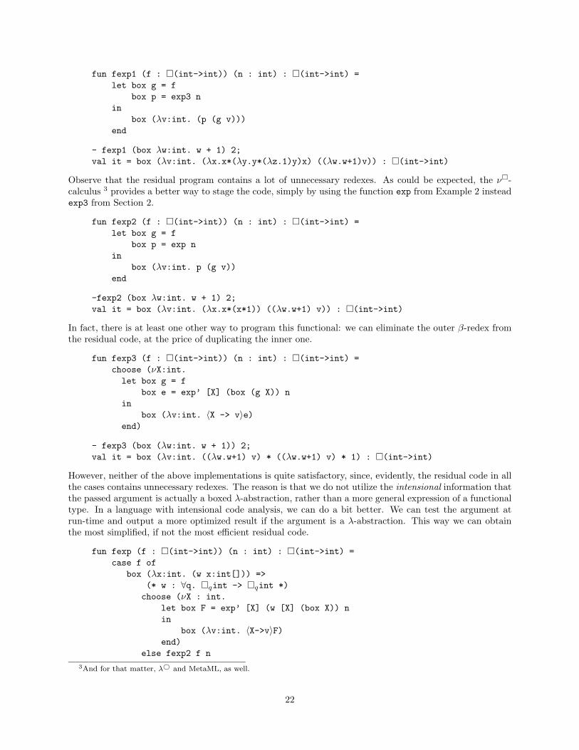
fun fexp1 (f : �(int->int)) (n : int) : �(int->int) =let box g = f

box p = exp3 nin

box (λv:int. (p (g v)))end

- fexp1 (box λw:int. w + 1) 2;val it = box (λv:int. (λx.x*(λy.y*(λz.1)y)x) ((λw.w+1)v)) : �(int->int)

Observe that the residual program contains a lot of unnecessary redexes. As could be expected, the ν�-calculus 3 provides a better way to stage the code, simply by using the function exp from Example 2 insteadexp3 from Section 2.

fun fexp2 (f : �(int->int)) (n : int) : �(int->int) =let box g = f

box p = exp nin

box (λv:int. p (g v))end

-fexp2 (box λw:int. w + 1) 2;val it = box (λv:int. (λx.x*(x*1)) ((λw.w+1) v)) : �(int->int)

In fact, there is at least one other way to program this functional: we can eliminate the outer β-redex fromthe residual code, at the price of duplicating the inner one.

fun fexp3 (f : �(int->int)) (n : int) : �(int->int) =choose (νX:int.let box g = f

box e = exp’ [X] (box (g X)) nin

box (λv:int. 〈X -> v〉e)end)

- fexp3 (box (λw:int. w + 1)) 2;val it = box (λv:int. ((λw.w+1) v) * ((λw.w+1) v) * 1) : �(int->int)

However, neither of the above implementations is quite satisfactory, since, evidently, the residual code in allthe cases contains unnecessary redexes. The reason is that we do not utilize the intensional information thatthe passed argument is actually a boxed λ-abstraction, rather than a more general expression of a functionaltype. In a language with intensional code analysis, we can do a bit better. We can test the argument atrun-time and output a more optimized result if the argument is a λ-abstraction. This way we can obtainthe most simplified, if not the most efficient residual code.

fun fexp (f : �(int->int)) (n : int) : �(int->int) =case f of

box (λx:int. (w x:int[])) =>(* w : ∀q. �qint -> �qint *)choose (νX : int.

let box F = exp’ [X] (w [X] (box X)) nin

box (λv:int. 〈X->v〉F)end)

else fexp2 f n

3And for that matter, λ© and MetaML, as well.

22

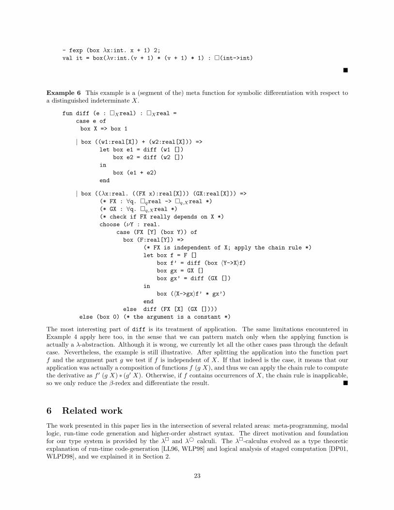
- fexp (box λx:int. x + 1) 2;val it = box(λv:int.(v + 1) * (v + 1) * 1) : �(int->int)

�

Example 6 This example is a (segment of the) meta function for symbolic differentiation with respect toa distinguished indeterminate X.

fun diff (e : �Xreal) : �Xreal =case e ofbox X => box 1

| box ((w1:real[X]) + (w2:real[X])) =>let box e1 = diff (w1 [])

box e2 = diff (w2 [])in

box (e1 + e2)end

| box ((λx:real. ((FX x):real[X])) (GX:real[X])) =>(* FX : ∀q. �qreal -> �q,Xreal *)(* GX : ∀q. �q,Xreal *)(* check if FX really depends on X *)choose (νY : real.

case (FX [Y] (box Y)) ofbox (F:real[Y]) =>

(* FX is independent of X; apply the chain rule *)let box f = F []

box f’ = diff (box 〈Y->X〉f)box gx = GX []box gx’ = diff (GX [])

inbox (〈X->gx〉f’ * gx’)

endelse diff (FX [X] (GX [])))

else (box 0) (* the argument is a constant *)

The most interesting part of diff is its treatment of application. The same limitations encountered inExample 4 apply here too, in the sense that we can pattern match only when the applying function isactually a λ-abstraction. Although it is wrong, we currently let all the other cases pass through the defaultcase. Nevertheless, the example is still illustrative. After splitting the application into the function partf and the argument part g we test if f is independent of X. If that indeed is the case, it means that ourapplication was actually a composition of functions f (g X), and thus we can apply the chain rule to computethe derivative as f ′ (g X) ∗ (g′ X). Otherwise, if f contains occurrences of X, the chain rule is inapplicable,so we only reduce the β-redex and differentiate the result. �

6 Related work

The work presented in this paper lies in the intersection of several related areas: meta-programming, modallogic, run-time code generation and higher-order abstract syntax. The direct motivation and foundationfor our type system is provided by the λ� and λ© calculi. The λ�-calculus evolved as a type theoreticexplanation of run-time code-generation [LL96, WLP98] and logical analysis of staged computation [DP01,WLPD98], and we explained it in Section 2.

23

The calculus λ©, formulated by Davies in [Dav96], is the first attempt at handling object expressionswith free variables. It is the proof-term calculus for discrete temporal logic, and it provides a notion of openobject expression where the free variables of the object expression are represented by meta variables on asubsequent temporal level. The original motivation of λ© was to develop a type system for binding-timeanalysis in the setup of partial evaluation, but it was quickly adopted for meta-programming through thedevelopment of MetaML [MTBS99, Tah99, Tah00].

MetaML adopts the “open code” type constructor of λ© and generalizes the language with severalfeatures. The most important one is the addition of a type refinement for “closed code”. Values classified bythese “closed code” types are those “open code” expressions which happen to not depend on any free metavariables. It might be of interest here to point out a certain relationship between our concept of names andthe phenomenon which occurs in the extension of MetaML with references [CMT00, CMS01]. A reference inMetaML must not be assigned an open code expression. Indeed, in such a case an eventual free variable fromthe expression may escape the scope of the λ-binder that introduced it. For technical reasons, however, thisactually cannot be prohibited, so the authors resort to a hygienic handling of scope extrusion by annotatinga term with the list of free variables that it is allowed to contain in dead-code positions. These dead-codeannotations are not a type constructor in MetaML, and the dead-code variables belong to the same syntacticcategory as ordinary variables, but they nevertheless very much compare to our names and ν-abstraction.Thus, it seems that names are important for meta-programming, even if one is not interested in intensionalcode analysis.

Another interesting calculus for meta-programming is Nielsen’s λ[] described in [Nie01]. It is based onthe same idea as our ν�-calculus – instead of defining the notion of closed code as a refinement of opencode of λ© or MetaML, it relaxes the notion of closed code of λ�. Where we use names to stand for freevariables of object expression, λ[] uses variables introduced by box (which thus becomes a binding construct).Variables bound by box have the same treatment as λ-bound variables. The type-constructor � is updatedto reflect the types (but not the names) of variables that its corresponding box binds, and thus it becomesquestionable whether it can be used for intensional analysis of higher-order syntax. The language also lacks aconcept corresponding to our support polymorphism which is one of the important ingredients for intensionalanalysis.

Nielsen and Taha in [NT03] present another system for combining the notions of closed and open code. Itis based on λ� but it can explicitly name the object stages of computation through the notion of environmentclassifiers. Because the stages are explicitly named, each stage can be revisited multiple times and extendedwith new bound variables. This provides a functionality of open code. In many respects, the environmentclassifiers behave like universally quantified bound variables. In fact, it seems that environment classifiersand our support polymorphism are formalizing the same phenomenon in different base calculi.

Coming from the direction of higher-order abstract syntax [PE88], probably the first work pointing to theimportance of a “non-parametric” binder like our ν-abstraction is Miller’s [Mil90]. The connection of higher-order abstract syntax to modal logic has been recognized by Despeyroux, Pfenning and Schurmann in thesystem presented in [DPS97], which was later simplified into a two-level system in Schurmann’s dissertation[Sch00]. There are also the works of Hofmann [Hof99], which discusses various presheaf models for higher-order abstract syntax, then Fiore, Plotkin and Turi’s [FPT99] which explores untyped abstract syntax in acategorical setup, and an extension to arbitrary types by Fiore [Fio02].

However, the work that explicitly motivated our developments is the series of papers on Nominal Logicand FreshML by Pitts and Gabbay [GP02, PG00, Pit01, Gab00]. The names of Nominal Logic are introducedas the urelements of Fraenkel-Mostowsky set theory. FreshML is a language for manipulation of object syntaxwith binding structure based on this model. Its primitive notion is that of swapping of two names which isthen used to define the operations of name abstraction (producing an α-equivalence class with respect to theabstracted name) and name concretion (providing a specific representative of an α-equivalence class). Theearlier version of our paper [Nan02] contained these two operations, which were almost orthogonal to add.Name abstraction was used to encode abstract syntax trees which depend on a name whose identity is notknown. Typically, the need for this would appear during pattern-matching of λ-binders when a new namemust be introduced to stand for the bound variable. Since this name is out of the scope of the subsequentcomputation branch, it has to be abstracted. In the current version, that role is given to λ-abstraction andsupport polymorphism as illustrated in Example 4.

24

Unlike our calculus, FreshML does not keep track of a support of a term, but rather its complement.FreshML introduces names in a computation by a construct new X in e, which can roughly be interpretedin ν�-calculus as

new X in e = choose (νX. e)

Except in dead-code position, the name X can appear in e in a scope of an abstraction which hides X.One of the main differences between FreshML and ν� is that names in FreshML are run-time values – itis possible in FreshML to evaluate a term with a non-empty support. On the other hand, while our namescan have arbitrary types, FreshML names must be of a single type atm (though this can be generalizedto an arbitrary family of types disjoint from the types of the other values of the language). Our calculusallows the general typing for names thanks to the modal distinction of meta and object levels. For example,without the modality, but with names of arbitrary types, a function defined on integers will always have toperform run-time checks to test if its argument is a valid integer (in which case the function is applied), orif its argument is a name (in which case the evaluation is suspended, and the whole expression becomes asyntactic entity). An added bonus is that ν� can support an explicit name substitution as primitive, whilesubstitution must be user-defined in FreshML.

On the logic side, the direct motivation for this paper comes from Pfenning and Davies’ [PD01] whichpresents a natural deduction formulation for propositional S4. But in general, the interaction betweenmodalities, syntax and names has been of interest to logicians for quite some time. For example, logics thatcan encode their own syntax are the topic of Godel’s Incompleteness theorems, and some references in thatdirection are Montague’s [Mon63] and Smorynski’s [Smo85]. Attardi’s viewpoints [AS95] and McCarthy’scontexts [McC93] are similar to our notion of support, and are used to express relativized truth. Finally,the names from ν� resemble virtual individuals of Scott [Sco70] and also [Sco79], non-rigid designators ofFitting and Mendelsohn [FM99], and names of Kripke [Kri80]. All this classical work seems to indicate thatmeta-programming and higher-order syntax are just but a concrete instance of a much broader abstractphenomenon. We hope to draw on the cited work for future developments.

7 Conclusions and future work

This paper presents the ν�-calculus, which is a typed functional language for meta-programming, employinga novel way to define a modal type of syntactic object programs with free variables. The system combinesthe λ�-calculus [PD01] with the notion of names inspired by developments in FreshML and Nominal Logic[PG00, GP02, Pit01, Gab00]. The motivation for combining λ� with names comes from the long-recognizedneed of meta-programming to handle object programs with free variables [Dav96, Tah99, MTBS99]. Inour setup, the λ�-calculus provides a way to encode closed syntactic code expressions, and names serve tostand for the eventual free variables. Taken together, they give us a way to encode open syntactic programexpressions, and also compose, evaluate, inspect and destruct them. Names can be operationally thought ofas locations which are tracked by the type system, so that names cannot escape the scope of their introductionform. The set of names appearing in the meta level of a term is called support of a term. Support of a termis reflected in the typing of a term, and a term can be evaluated only if its support is empty.

We also considered constructs for support polymorphism and for intensional analysis of higher-ordersyntax. The later is a pattern-matching mechanism to compare, inspect and destruct object expressions atrun-time. We hope this feature can find its use in programming code optimizations in a setup of scientificand symbolic computation.

The ν�-calculus presented here supersedes the language considered in the previous version of this paper[Nan02]. Some of the changes we have adopted involve simplification of the operational semantics and theconstructs for handling names. Furthermore, we decomposed the name introduction form new into two newconstructors ν and choose which are now introduction and elimination form for a new type constructorA9 B. This gives a stronger logical foundation to the calculus, as now the level of types follows much moreclosely the behavior of the terms of the language. We hope to further investigate these logical properties.Some immediate future work in this direction would include the embedding of discrete-time temporal logicand monotone discrete temporal logic into the logic of types of ν�, and also considering the proof-irrelevancymodality of [Pfe01] and [AB01] to classify terms of unknown support.

25

8 Acknowledgment

First and foremost, I would like to thank my advisor Frank Pfenning for all his invaluable contributions tothis work, his strategic guidance and, above all, his tireless support. This document would have never seenthe light without him. I am also indebted to Dana Scott, Bob Harper, Peter Lee and Andrew Pitts for theirhelpful comments on the earlier version of the paper.

References

[AB01] Steve Awodey and Andrej Bauer. Propositions as [Types]. Technical Report IML-R–34-00/01–SE, Institut Mittag-Leffler, The Royal Swedish Academy of Sciences, 2001.

[AS95] Giuseppe Attardi and Maria Simi. A formalization of viewpoints. Fundamenta Informaticae,23(3):149–173, 1995.

[BES98] Ulrich Berger, Matthias Eberl, and Helmut Schwichtenberg. Normalization by evaluation. InBernhard Moller and John V. Tucker, editors, Prospects for Hardware Foundations, volume 1546of Lecture Notes in Computer Science, pages 117–137. Springer, 1998.

[BS91] Ulrich Berger and Helmut Schwichtenberg. An inverse of the evaluation functional for typedlambda-calculus. In LICS’91: Logic in Computer Science, pages 203–211, Amsterdam, 1991.

[CMS01] Cristiano Calcagno, Eugenio Moggi, and Tim Sheard. Closed types for a safe imperative MetaML.Journal of Functional Programming, 2001. To appear.

[CMT00] Cristiano Calcagno, Eugenio Moggi, and Walid Taha. Closed types as a simple approach to safeimperative multi-stage programming. In Ugo Montanari, Jose D. P. Rolim, and Emo Welzl,editors, Automata, Languages and Programming, volume 1853 of Lecture Notes in ComputerScience, pages 25–36. Springer, 2000.

[Dan96] Olivier Danvy. Type-directed partial evaluation. In POPL’96: Principles of Programming Lan-guages, pages 242–257, St. Petersburg Beach, Florida, 1996.

[Dav96] Rowan Davies. A temporal logic approach to binding-time analysis. In LICS’96: Logic inComputer Science, pages 184–195, New Brunswick, New Jersey, 1996.

[DP01] Rowan Davies and Frank Pfenning. A modal analysis of staged computation. Journal of theACM, 48(3):555–604, 2001.

[DPS97] Joelle Despeyroux, Frank Pfenning, and Carsten Schurmann. Primitive recursion for higher-orderabstract syntax. In Philippe de Groote and J. Roger Hindley, editors, Typed Lambda Calculi andApplications, volume 1210 of Lecture Notes in Computer Science, pages 147–163. Springer, 1997.

[Fio02] Marcelo Fiore. Semantic analysis of normalization by evaluation for typed lambda calculus.In PPDP’02: Principles and Practice of Declarative Programming, pages 26–37, Pittsburgh,Pennsylvania, 2002.

[FM99] Melvin Fitting and Richard L. Mendelsohn. First-Order Modal Logic. Kluwer, 1999.

[FPT99] Marcelo Fiore, Gordon Plotkin, and Daniele Turi. Abstract syntax and variable binding. InLICS’99: Logic in Computer Science, pages 193–202, Trento, Italy, 1999.

[Gab00] Murdoch J. Gabbay. A Theory of Inductive Definitions with α-Equivalence. PhD thesis, Cam-bridge University, August 2000.

[Gir86] Jean-Yves Girard. The system F of variable types, fifteen years later. Theoretical ComputerScience, 45(2):159–192, 1986.

26

[GP02] Murdoch J. Gabbay and Andrew M. Pitts. A new approach to abstract syntax with variablebinding. Formal Aspects of Computing, 13:341–363, 2002.

[Gri89] Andreas Griewank. On automatic differentiation. In Masao Iri and Kunio Tanabe, editors,Mathematical Programming: Recent Developments and Applications, pages 83–108. Kluwer, 1989.

[Hof99] Martin Hofmann. Semantical analysis of higher-order abstract syntax. In LICS’99: Logic inComputer Science, pages 204–213, Trento, Italy, 1999.

[Kri80] Saul A. Kripke. Naming and Necessity. Harvard University Press, 1980.

[LL96] Peter Lee and Mark Leone. Optimizing ML with run-time code generation. In PLDI’96: Pro-gramming Language Design and Implementation, pages 137–148, 1996.

[McC93] John McCarthy. Notes on formalizing context. In IJCAI’93: International Joint Conference onArtificial Intelligence, pages 555–560, Chambery, France, 1993.

[Mil90] Dale Miller. An extension to ML to handle bound variables in data structures. In Proceedings ofthe First Esprit BRA Workshop on Logical Frameworks, pages 323–335, Antibes, France, 1990.

[Mon63] Richard Montague. Syntactical treatment of modalities, with corollaries on reflexion principlesand finite axiomatizability. Acta Philosophica Fennica, 16:153–167, 1963.

[MTBS99] Eugenio Moggi, Walid Taha, Zine-El-Abidine Benaissa, and Tim Sheard. An idealized MetaML:Simpler, and more expressive. In ESOP’99: European Symposium on Programming, pages 193–207, Amsterdam, 1999.

[Nan02] Aleksandar Nanevski. Meta-programming with names and necessity. In ICFP’02: InternationalConference on Functional Programming, pages 206–217, Pittsburgh, Pennsylvania, 2002.

[Nie01] Michael Florentin Nielsen. Combining closed and open code. Unpublished, 2001.

[NT03] Michael Florentin Nielsen and Walid Taha. Environment classifiers. In POPL’03: Principles ofProgramming Languages, New Orleans, Louisiana, 2003. To appear.

[Ode94] Martin Odersky. A functional theory of local names. In POPL’94: Principles of ProgrammingLanguages, pages 48–59, Portland, Oregon, 1994.

[PD01] Frank Pfenning and Rowan Davies. A judgmental reconstruction of modal logic. MathematicalStructures in Computer Science, 11(4):511–540, 2001.

[PE88] Frank Pfenning and Conal Elliott. Higher-order abstract syntax. In PLDI’88: ProgrammingLanguage Design and Implementation, pages 199–208, Atlanta, Georgia, 1988.

[Pfe01] Frank Pfenning. Intensionality, extensionality, and proof irrelevance in modal type theory. InLICS’01: Logic in Computer Science, pages 221–230, Boston, Massachusetts, 2001.

[PG00] Andrew M. Pitts and Murdoch J. Gabbay. A metalanguage for programming with bound namesmodulo renaming. In Roland Backhouse and Jose Nuno Oliveira, editors, Mathematics of Pro-gram Construction, volume 1837 of Lecture Notes in Computer Science, pages 230–255. Springer,2000.

[Pit01] Andrew M. Pitts. Nominal logic: A first order theory of names and binding. In Naoki Kobayashiand Benjamin C. Pierce, editors, Theoretical Aspects of Computer Software, volume 2215 ofLecture Notes in Computer Science, pages 219–242. Springer, 2001.

[Rey83] John C. Reynolds. Types, abstraction and parametric polymorphism. In R. E. A. Mason, editor,Information Processing ’83, pages 513–523. Elsevier, 1983.

[Roz93] Guillermo J. Rozas. Translucent procedures, abstraction without opacity. Technical ReportAITR-1427, Massachusetts Institute of Technology Artificial Intelligence Laboratory, 1993.

27

[RP02] Norman Ramsey and Avi Pfeffer. Stochastic lambda calculus and monads of probability distri-butions. In POPL’02: Principles of Programming Languages, pages 154–165, Portland, Oregon,2002.

[Sch00] Carsten Schurmann. Automating the Meta-Theory of Deductive Systems. PhD thesis, CarnegieMellon University, 2000.

[Sco70] Dana Scott. Advice on modal logic. In Karel Lambert, editor, Philosophical Problems in Logic,pages 143–173. Dordrecht: Reidel, 1970.

[Sco79] Dana Scott. Identity and existence in intuitionistic logic. In Michael Fourman, Chris Mulvey,and Dana Scott, editors, Applications of Sheaves, volume 753 of Lecture Notes in Mathematics,pages 660–696. Springer, 1979.

[She01] Tim Sheard. Accomplishments and research challenges in meta-programming. In Walid Taha,editor, Semantics, Applications, and Implementation of Program Generation, volume 2196 ofLecture Notes in Computer Science, pages 2–44. Springer, 2001.

[Smo85] C. Smorynski. Self-Reference and Modal Logic. Springer, 1985.

[Tah99] Walid Taha. Multi-Stage Programming: Its Theory and Applications. PhD thesis, Oregon Grad-uate Institute of Science and Technology, 1999.

[Tah00] Walid Taha. A sound reduction semantics for untyped CBN multi-stage computation. Or, thetheory of MetaML is non-trival. In PEPM’00: Partial Evaluation and Semantics-Based ProgramManupulation, pages 34–43, Boston, Massachusetts, 2000.

[WLP98] Philip Wickline, Peter Lee, and Frank Pfenning. Run-time code generation and Modal-ML.In PLDI’98: Programming Language Design and Implementation, pages 224–235, Montreal,Canada, 1998.

[WLPD98] Philip Wickline, Peter Lee, Frank Pfenning, and Rowan Davies. Modal types as staging specifi-cations for run-time code generation. ACM Computing Surveys, 30(3es), 1998.

A Proofs

A.1 Structural properties

Lemma 5 (Support weakening)Let C ⊆ C ′ ⊆ dom(Σ) and D′ ⊆ D ⊆ dom(Σ) be well-formed support sets. Then the following holds:

1. if Σ; ∆; Γ ` e : A [C], then Σ; ∆; Γ ` e : A [C ′].

2. if Σ; ∆; Γ ` 〈Θ〉 : [D]⇒ [C], then Σ; ∆; Γ ` 〈Θ〉 : [D]⇒ [C ′].

3. if Σ; (∆, u:A[D]); Γ ` e : B [C], then Σ; (∆, u:A[D′]); Γ ` e : B [C]

4. if Σ; ∆; Γ ` 〈Θ〉 : [D]⇒ [C], then Σ; ∆; Γ ` 〈Θ〉 : [D′]⇒ [C].

Proof: The first two statements are proved by straightforward simultaneous induction on the given deriva-tions. We present only selected cases.

1. case e = 〈Θ〉u.

(a) by derivation, u:A[C ′′] ∈ ∆ and Σ; ∆; Γ ` 〈Θ〉 : [C ′′]⇒ [C](b) by 2. Σ; ∆; Γ ` 〈Θ〉 : [C ′′]⇒ [C ′](c) result follows by typing

28

2. case Θ = (·)By derivation, D ⊆ C ⊆ C ′ so the result follows by the typing rules.

case Θ = (X → e′,Θ′).

(a) by derivation, Σ; ∆; Γ ` e′ : A [C] and Σ; ∆; Γ ` 〈Θ′〉 : [D \ {X}]⇒ [C](b) by 1. Σ; ∆; Γ ` e′ : A [C ′](c) by induction hypothesis, Σ; ∆; Γ ` 〈Θ′〉 : [D \ {X}]⇒ [C ′](d) result follows by typing

3. Induction on the structure of the derivation.

case e = 〈Θ〉u.

(a) by derivation, Σ; (∆, u:A[D]); Γ ` 〈Θ〉 : [D]⇒ [C](b) by induction on the structure of Θ, we get Σ; (∆, u:A[D]); Γ ` 〈Θ〉 : [D]⇒ [C](c) by 4. Σ; (∆, u:A[D]); Γ ` 〈Θ〉 : [D′]⇒ [C](d) result follows by typing

4. Induction on the structure of the derivation.

case Θ = (·). Then D′ ⊆ D ⊆ C.

case Θ = (X → e,Θ′).

(a) by derivation, Σ; ∆; Γ ` 〈Θ′〉 : [D \ {X}]⇒ [C] and Σ; ∆; Γ ` e : A [C](b) by induction hypothesis, Σ; ∆; Γ ` 〈Θ′〉 : [D′ \ {X}]⇒ [C](c) result follows by typing

�

Lemma 6 (Support extension)Let D ⊆ dom(Σ) be a well-formed support set. Then the following holds:

1. if Σ; (∆, u:A[C1]); Γ ` e : B [C2] then Σ; (∆, u:A[C1 ∪D]); Γ ` e : B [C2 ∪D]

2. if Σ; ∆; Γ ` 〈Θ〉 : [C1]⇒ [C2], then Σ; ∆; Γ ` 〈Θ〉 : [C1 ∪D]⇒ [C2 ∪D]

Proof:

1. By induction on the structure of the derivation.

case e = x,X is trivially true by support weakening.

case e = 〈Θ〉u, where A = B.

(a) by derivation, Σ; (∆, u:A[C1]); Γ ` 〈Θ〉 : [C1]⇒ [C2](b) by induction on the structure of Θ, we get Σ; (∆, u:A[C1 ∪D]); Γ ` 〈Θ〉 : [C1]⇒ [C2 ∪D](c) by 2. Σ; (∆;u:A[C1 ∪D]); Γ ` 〈Θ〉 : [C1 ∪D]⇒ [C2 ∪D](d) result follows by typing

2. By induction on the structure of the derivation.

case Θ = (X → e,Θ′), where X:A ∈ Σ.

(a) by derivation, Σ; ∆; Γ ` e : A [C2] and Σ; ∆; Γ ` 〈Θ′〉 : [C1 \ {X}]⇒ [C2](b) by support weakening, Σ; ∆; Γ ` e : A [C2 ∪D](c) by induction hypothesis and support weakening, Σ; ∆; Γ ` 〈Θ′〉 : [(C1 ∪D) \ {X}]⇒ [C2 ∪D](d) result follows by typing

29

�

Lemma 7 (Substitution merge)If Σ; ∆; Γ ` 〈Θ〉 : [C1] ⇒ [D] and Σ; ∆; Γ ` 〈Θ′〉 : [C2] ⇒ [D] where dom(Θ) ∩ dom(Θ′) = ∅, then〈Θ,Θ′〉 : [C1 ∪ C2]⇒ [D].Proof: By induction on the structure of Θ′.

case Θ′ = (·). Then C2 ⊆ D and results follow by support extension (Lemma 6.2).

case Θ′ = (X → e,Θ′1).

1. by derivation, Σ; ∆; Γ ` 〈Θ′1〉 : [C2 \ {X}]⇒ [D]

2. by induction hypothesis, Σ; ∆; Γ ` 〈Θ,Θ′1〉 : [C1 ∪ (C2 \ {X})]⇒ [D]

3. by support weakening, Σ; ∆; Γ ` 〈Θ,Θ′1〉 : [(C1 ∪ C2) \ {X}]⇒ [D]

4. result follows by typing

�

A.2 Substitution principles

Lemma 8 (Explicit substitution principle)Let Σ; ∆; Γ ` 〈Θ〉 : [C]⇒ [D]. Then the following holds:

1. if Σ; ∆; Γ ` e : A [C] then Σ; ∆; Γ ` {Θ}e : A [D].

2. if Σ; ∆; Γ ` 〈Θ′〉 : [C1]⇒ [C], then Σ; ∆; Γ ` 〈Θ ◦Θ′〉 : [C1]⇒ [D].

Proof: By simultaneous induction on the structure of the derivations. We just present selected cases.

1. case e = x. The judgment is derived by weakening at the hypothesis, so we can also derive x:A[D].This is sufficient, as {Θ}x = x.

case e = 〈Θ′〉u.

(a) by derivation, u : A [C1] ∈ ∆ and Σ; ∆; Γ ` 〈Θ′〉 : [C1]⇒ [C].(b) by 2. Σ; ∆; Γ ` 〈Θ ◦Θ′〉 : [C1]⇒ [D].(c) result follows by typing

case e = X, where X:A ∈ Σ.

(a) by derivation, X ∈ C.(b) if X ∈ dom(Θ) with e′ = Θ (X), then by typing of Θ, Σ; ∆; Γ ` e′ : A [D](c) if X 6∈ dom(Θ), then by derivation of Θ, it must be X ∈ D since we assumed X ∈ C(d) by support weakening, Σ; ∆; Γ ` X : A [D](e) result follows by typing

2. Given the substitutions Θ and Θ′, we split the representation of Θ ◦Θ′ into two disjoint sets:

Θ′1 = {X → Θ(X) | X ∈ dom(Θ) \ dom(Θ′)}Θ′2 = {X → {Θ}(Θ′X) | X ∈ dom(Θ′)}

and set out to show that

(a) Σ; ∆; Γ ` 〈Θ′1〉 : [C1 \ dom(Θ′)]⇒ [D], and

(b) Σ; ∆; Γ ` 〈Θ′2〉 : [C1 ∩ dom(Θ′)]⇒ [D].

30

These two typings imply the result by the substitution merge lemma (Lemma 7). The statement (b)follows from the typing of Θ′ by support weakening (Lemma 5.4), and the first part of the lemma. Toestablish (a), observe that from the typing of Θ it is clear that Θ′1 : [C \ dom(Θ′)]⇒ [D]. But, sinceC1 \ dom(Θ′) ⊆ C \ dom(Θ′) readily follows from the typing of Θ′, the result is obtained by supportweakening.

�

Lemma 9 (Value substitution principle)Let Σ; ∆; Γ ` e1 : A [C]. The following holds:

1. if Σ; ∆; (Γ, x:A) ` e2 : B [C], then Σ; ∆; Γ ` [e1/x]e2 : B [C]

2. if Σ; ∆; (Γ, x:A) ` 〈Θ〉 : [C ′]⇒ [C], then Σ; ∆; Γ ` 〈[e1/x]Θ〉 : [C ′]⇒ [C]

Proof: Simultaneous induction on the two derivations.

1. case e2 = x,X obvious.

case e2 = 〈Θ〉u.

(a) by derivation, Σ; ∆; (Γ, x:A) ` 〈Θ〉 : [C ′]⇒ [C] and u : B [C ′] ∈ ∆.(b) by 2., Σ; ∆; Γ ` 〈[e1/x]Θ〉 : [C ′]⇒ [C](c) result follows by typing.

case e2 = λy:B′. e′, where B = B′ → B′′.

(a) by derivation, Σ; ∆; (Γ, x:A, y:B′) ` e′ : B′′ [C](b) by induction hypothesis, Σ; ∆; (Γ, y:B′) ` [e1/x]e′ : B′′ [C](c) result follows by typing

case e2 = e′ e′′.

(a) by derivation, Σ; ∆; (Γ, x:A) ` e′ : B′ → B [C] and Σ; ∆; (Γ, x:A) ` e′′ : B′ [C](b) by induction hypothesis, Σ; ∆; Γ ` [e1/x]e′ : B′ → B [C], and Σ; ∆; Γ ` [e1/x]e′′ : B′ [C](c) result follows by typing

case e2 = box e′.Trivial, since x 6∈ fv(e′).

case e2 = let box u = e′ in e′′.

(a) by derivation, Σ; ∆; (Γ, x:A) ` e′ : �C′B′ [C] and Σ; (∆, u:B′[C ′]); (Γ, x:A) ` e′′ : B [C](b) by induction hypothesis, Σ; ∆; Γ ` [e1/x]e′ : �C′B′ [C] and Σ; (∆, u:B′[C ′]); Γ ` [e1/x]e′′ :

B [C].(c) result follows by typing

case e2 = νX:B′. e′, where B = B′ 9 B′′.

(a) by derivation, (Σ, X:B′); ∆; (Γ, x:A) ` e′ : B′′ [C] and X 6∈ fn(B′′[C])(b) by induction hypothesis, (Σ, X:B′); ∆; Γ ` [e1/x]e′ : B′′ [C](c) result follows by typing

case e2 = choose e′, where Σ = (Σ′, X:B′).

(a) by derivation, Σ′; ∆; (Γ, x:A) ` e′ : B′ 9 B [C](b) by induction hypothesis, Σ′; ∆; Γ ` [e1/x]e′ : B′ 9 B [C](c) result follows by typing

case e2 = Λp. e′ where B = ∀p. B′.(a) by derivation, (Σ, p); ∆; (Γ, x:A) ` e′ : B′ [C](b) by induction hypothesis, (Σ, p); ∆; Γ ` [e1/x]e′ : B′ [C]

31

(c) result follows by typing

case e2 = e′ [C ′], where B = [C ′/p]B′.

(a) by derivation, Σ; ∆; (Γ, x:A) ` e′ : ∀p. B′ [C](b) by induction hypothesis, Σ; ∆; Γ ` [e1/x]e′ : ∀p. B′ [C](c) result follows by typing

case e2 = case e′ of box π ⇒ e′1 else e′2.

(a) by derivation:i. Σ; ∆; (Γ, x:A) ` e′ : �DA1 [C]ii. Σ; · ` π : A1 [D] =⇒ Γ1

iii. Σ; ∆; (Γ, x:A,Γ1) ` e′1 : B [C]iv. Σ; ∆; (Γ, x:A) ` e′2 : B [C]

(b) by induction hypothesis:i. Σ; ∆; Γ ` [e1/x]e′ : �DA1 [C]ii. Σ; ∆; (Γ,Γ1) ` [e1/x]e′1 : B [C]iii. Σ; ∆; Γ ` [e1/x]e′2 : B [C]

(c) result follows by typing

2. case Θ = (·) is trivial.

case Θ = (X → e′,Θ′).

(a) by derivation, Σ; ∆; (Γ, x:A) ` e′ : B′ [C] and Σ; ∆; (Γ, x:A) ` 〈Θ′〉 : [C ′ \ {X}]⇒ [C](b) by 1. Σ; ∆; Γ ` [e1/x]e′ : B′ [C](c) by induction hypothesis, Σ; ∆; Γ ` 〈[e1/x]Θ′〉 : [C ′ \ {X}]⇒ [C](d) result follows by typing

�

Lemma 11 (Expression substitution principle)Let e1 be an expression without free value variables such that Σ; ∆; · ` e1 : A [C]. Then the following holds:

1. if Σ; (∆, u:A[C]); Γ ` e2 : B [D], then Σ; ∆; Γ ` [[e1/u]]e2 : B [D]

2. if Σ; (∆, u:A[C]); Γ ` 〈Θ〉 : [D′]⇒ [D], then Σ; ∆; Γ ` 〈[[e1/u]]Θ〉 : [D′]⇒ [D]

Proof:

1. By simultaneous induction on the two derivations.

case e2 = x,X obvious.

case e2 = 〈Θ〉u.

(a) by derivation, A = B and Σ; (∆, u:A[C]); Γ ` 〈Θ〉 : [C]⇒ [D](b) by 2. Σ; ∆; Γ ` 〈[[e1/u]]Θ〉 : [C]⇒ [D](c) by principle of explicit substitution (Lemma 8.1), Σ; ∆; Γ ` {[[e1/u]]Θ}e1 : B [D](d) but this is exactly equal to [[e1/u]]e2

case e2 = 〈Θ〉v, where v:B[D′] ∈ ∆

(a) by derivation, Σ; (∆, u:A[C]); Γ ` 〈Θ〉 : [D′]⇒ [D](b) by 2., Σ; ∆; Γ ` 〈[[e1/u]]Θ〉 : [D′]⇒ [D](c) result follows by typing

case e2 = λx:B′. e′, where B = B′ → B′′.

32

(a) by derivation, Σ; (∆, u:A[C]); (Γ, x:B′) ` e′ : B′′ [D](b) by induction hypothesis, Σ; ∆; (Γ, x:B′) ` [[e1/u]]e′ : B′′ [D](c) result follows by typing

case e2 = e′ e′′.

(a) by derivation, Σ; (∆, u:A[C]); Γ ` e′ : B′ → B [D] and also Σ; (∆, u:A[C]); Γ ` e′′ : B′ [D](b) by induction hypothesis, Σ; ∆; Γ ` [[e1/u]]e′ : B′ → B [D], and also Σ; ∆; Γ ` [[e1/u]]e′′ : B′ [D](c) result follows by typing

case e2 = box e′, where B = �D′B′

(a) by derivation, Σ; (∆, u:A[C]); Γ ` e′ : B′ [D′](b) by induction hypothesis, Σ; ∆; Γ ` [[e1/u]]e′ : B′ [D′](c) result follows by typing

case e2 = let box v = e′ in e′′.

(a) by derivation, Σ; (∆, u:A[C]); Γ ` e′ : �D′B′ [D] and also Σ; (∆, u:A[C], v:B′[D′]); Γ ` e′′ :B [D]

(b) by induction hypothesis, Σ; ∆; Γ ` [[e1/u]]e′ : �D′B′ [D] and Σ; (∆, v:B′[D′]); Γ ` [[e1/u]]e′′ :B [D].

(c) result follows by typing

case e2 = νX:B′. e′, where B = B′ 9 B′′.

(a) by derivation, (Σ, X:B′); (∆, u:A[C]); Γ ` e′ : B′′ [D] and also X 6∈ fn(B′′[D])(b) by induction hypothesis, (Σ, X:B′); ∆; ∆ ` [[e1/u]]e′ : B′′ [D](c) result follows by typing

case e2 = choose e′, where Σ = (Σ′, X:B′).

(a) by derivation, Σ′; (∆, u:A[C]); Γ ` e′ : B′ 9 B [D](b) by induction hypothesis, Σ′; ∆; Γ ` [[e1/u]]e′ : B′ 9 B [D](c) result follows by typing

case e2 = Λp. e′ where B = ∀p. B′.(a) by derivation, (Σ, p); (∆, u:A[C]); Γ ` e′ : B′ [D](b) by induction hypothesis, (Σ, p); ∆; Γ ` [[e1/u]]e′ : B′ [D](c) result follows by typing

case e2 = e′ [D′], where B = [D′/p]B′.

(a) by derivation, Σ; (∆, u:A[C]); Γ ` e′ : ∀p. B′ [D](b) by induction hypothesis, Σ; ∆; Γ ` [[e1/u]]e′ : ∀p. B′ [D](c) result follows by typing

case e2 = case e′ of box π ⇒ e′1 else e′2.

(a) by derivation:i. Σ; (∆, u:A[C]); Γ ` e′ : �D′A1 [D]ii. Σ; · ` π : A1 [D′] =⇒ Γ1

iii. Σ; (∆, u:A[C]); (Γ,Γ1) ` e′1 : B [D]iv. Σ; (∆, u:A[C]); Γ ` e′2 : B [D]

(b) by induction hypothesis:i. Σ; ∆; Γ ` [[e1/u]]e′ : �D′A1 [D]ii. Σ; ∆; (Γ,Γ1) ` [[e1/u]]e′1 : B [D]iii. Σ; ∆; Γ ` [[e1/u]]e′2 : B [D]

33

(c) result follows by typing

2. case Θ = (·) is trivial.

case Θ = (X → e′,Θ′).

(a) by derivation, Σ; (∆, u:A[C]); Γ ` e′ : B′ [D] and also Σ; (∆, u:A[C]); Γ ` 〈Θ′〉 : [D′ \ {X}]⇒[D]

(b) by 1., Σ; ∆; Γ ` [[e1/u]]e′ : B′ [D](c) by induction hypothesis, Σ; ∆; Γ ` 〈[[e1/u]]Θ′〉 : [D′ \ {X}]⇒ [D](d) result follows by typing

�

Lemma 15 (Support substitution principle)Let Σ = (Σ1, p,Σ2) and D ⊆ dom(Σ1) and denote by (−)′ the operation of substituting D for p. Then thefollowing holds.

1. if Σ; ∆; Γ ` e : A [C], then (Σ1,Σ′2); ∆′; Γ′ ` e′ : A′ [C ′]

2. if Σ; ∆; Γ ` Θ : C1 → C2, then (Σ1,Σ′2); ∆′; Γ′ ` Θ′ : C ′1 → C ′2

Proof:

1. case e = x,X is trivial.

case e = 〈Θ〉u.

(a) by derivation Σ; ∆; Γ ` Θ : C1 → C and u:A[C1] ∈ ∆(b) by definition u:A′[C ′1] ∈ ∆′

(c) by 2. (Σ1,Σ′2); ∆′; Γ′ ` Θ′ : C ′1 → C ′

(d) result follows by typing

case e = λx:A1. e1 where A = A1 → A2.

(a) by derivation, Σ; ∆; (Γ, x:A1) ` e1 : A2 [C](b) by induction hypothesis, (Σ1,Σ′2); ∆′; (Γ′, x:A′1) ` e′1 : A′2 [C ′](c) result follows by typing

case e = e1 e2.

(a) by derivation, Σ; ∆; Γ ` e1 : A1 → A [C], and Σ; ∆; Γ ` e2 : A1 [C](b) by induction hypothesis (Σ1,Σ′2); ∆′; Γ′ ` e′1 : A′1 → A′ [C ′] and (Σ1,Σ′2); ∆′; Γ′ ` e′2 : A′1 [C ′](c) result follows by typing

case e = box e1, where A = �C1A1.

(a) by derivation, Σ; ∆; Γ ` e1 : A1 [C1](b) by induction hypothesis, (Σ1,Σ′2); ∆′; Γ′ ` e′1 : A′1 [C ′1](c) result follows by typing

case e = let box u = e1 in e2

(a) by derivation, Σ; ∆; Γ ` e1 : �C1A1 [C] and Σ; (∆, u:A1[C1]); Γ ` e2 : A [C](b) by induction hypothesis, (Σ1,Σ′2); ∆′; Γ′ ` e′1 : �C′1A

′1 [C ′] and (Σ1,Σ′2); (∆′, u:A′1[C ′1]); Γ′ `

e′2 : A′ [C ′](c) result follows by typing

case e = νX:A. e1 where A = A1 9 A2

(a) by derivation, (Σ, X:A); ∆; Γ ` e1 : A2 [C](b) by induction hypothesis (Σ1,Σ′2, X:A′); ∆′; Γ′ ` e′1 : A′2 [C ′]

34

(c) result follows by typing

case e = choose e1.

(a) by derivation, Σ; ∆; Γ ` e1 : A1 9 A [C](b) by induction hypothesis (Σ1,Σ′2); ∆′; Γ′ ` e′1 : A′1 9 A′ [C ′](c) result follows by typing

case e = Λq. e1 where A = ∀q. A1.

(a) by derivation, (Σ, q); ∆; Γ ` e1 : A1 [C](b) by induction hypothesis, (Σ1,Σ′2, q); ∆′; Γ′ ` e′1 : A′1 [C ′](c) result follows by typing

case e = e1 [C1].

(a) by derivation, Σ; ∆; Γ ` e1 : ∀q. A1 [C] and A = [C1/q]A1

(b) by induction hypothesis, (Σ1,Σ′2); ∆′; Γ′ ` e′1 : ∀q. A′1 [C ′](c) it is easy to see that [C ′1/q]A

′1 = ([C1/q]A1)′

(d) result follows by typing

case e = case e0 of box π ⇒ e1 else e2.

(a) by derivation:i. Σ; ∆; Γ ` e0 : �D1A1 [C]ii. Σ; · ` π : A1 [D1] =⇒ Γ1

iii. Σ; (Γ,Γ1) ` e1 : A [C]iv. Σ; Γ ` e2 : A [C]

(b) by induction hypothesis:i. (Σ1,Σ′2); ∆′; Γ′ ` e′0 : �D′1A

′1 [C ′]

ii. (Σ1,Σ′2); (Γ′,Γ′1) ` e′1 : A′ [C ′]iii. (Σ1,Σ′2); Γ′ ` e′2 : A′ [C ′]

(c) by principle of support substitution for pattern (Lemma 17), (Σ1,Σ′2); · ` π′ : A′1 [D′1] =⇒ Γ′1(d) result follows by typing

2. case Θ = (·) is trivial.

case Θ = (X → e1,Θ1), where X:B ∈ Σ.

(a) by derivation, Σ; ∆; Γ ` e1 : B [D] and Σ; ∆; Γ ` Θ1 : C1 \ {X} → C2

(b) by 1. (Σ1,Σ′2); ∆′; Γ′ ` e′1 : B′ [C ′2](c) by induction hypothesis, (Σ1,Σ′2); ∆′; Γ′ ` Θ′1 : C ′1 \ {X} → C ′2(d) result follows by typing

�

A.3 Operational semantics

Theorem 12 (Type preservation)If Σ; ·; · ` e : A [ ] and Σ, e 7−→ Σ′, e′, then Σ′; ·; · ` e′ : A [ ].Theorem 13 (Progress)If Σ; ·; · ` e : A [ ], then either

1. e is a value, or

2. there exist a term e′ and a context Σ′ extending Σ, such that Σ, e 7−→ Σ′, e′.

35

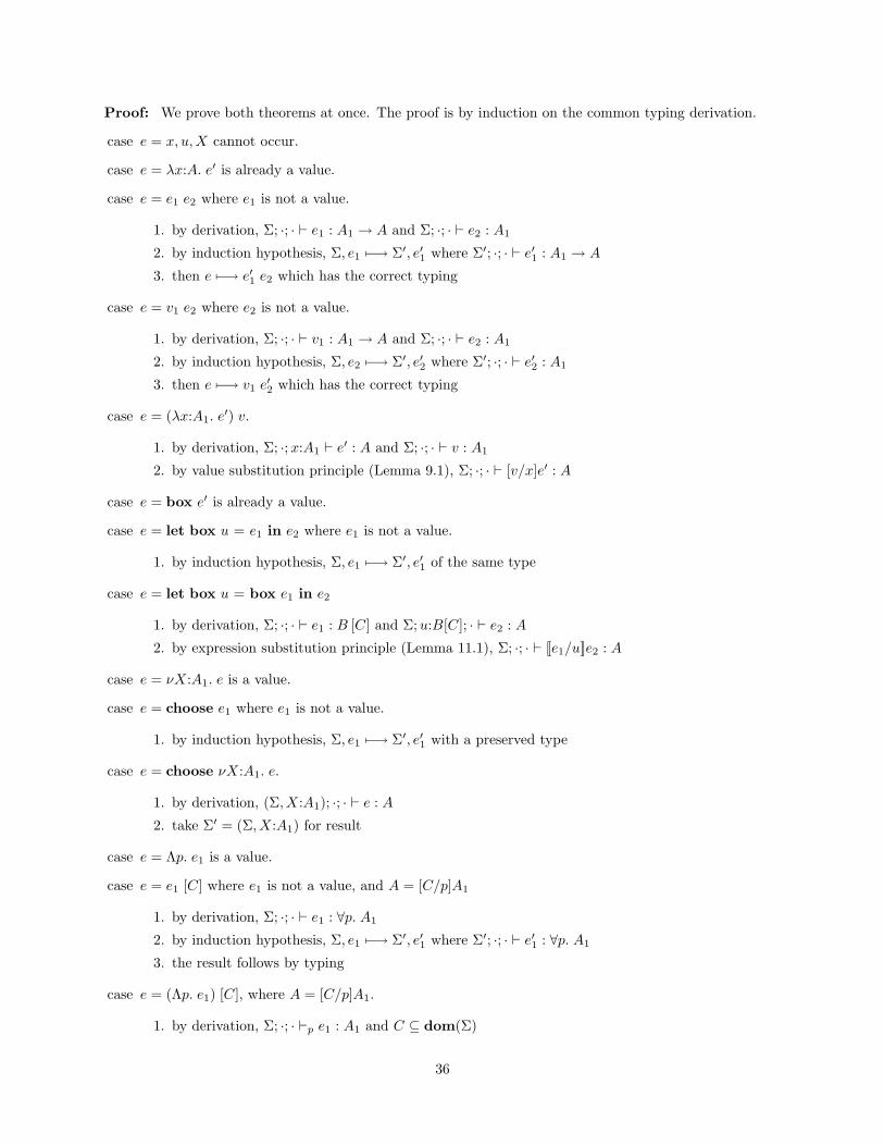
Proof: We prove both theorems at once. The proof is by induction on the common typing derivation.

case e = x, u,X cannot occur.

case e = λx:A. e′ is already a value.

case e = e1 e2 where e1 is not a value.

1. by derivation, Σ; ·; · ` e1 : A1 → A and Σ; ·; · ` e2 : A1

2. by induction hypothesis, Σ, e1 7−→ Σ′, e′1 where Σ′; ·; · ` e′1 : A1 → A

3. then e 7−→ e′1 e2 which has the correct typing

case e = v1 e2 where e2 is not a value.

1. by derivation, Σ; ·; · ` v1 : A1 → A and Σ; ·; · ` e2 : A1

2. by induction hypothesis, Σ, e2 7−→ Σ′, e′2 where Σ′; ·; · ` e′2 : A1

3. then e 7−→ v1 e′2 which has the correct typing

case e = (λx:A1. e′) v.

1. by derivation, Σ; ·;x:A1 ` e′ : A and Σ; ·; · ` v : A1

2. by value substitution principle (Lemma 9.1), Σ; ·; · ` [v/x]e′ : A

case e = box e′ is already a value.

case e = let box u = e1 in e2 where e1 is not a value.

1. by induction hypothesis, Σ, e1 7−→ Σ′, e′1 of the same type

case e = let box u = box e1 in e2

1. by derivation, Σ; ·; · ` e1 : B [C] and Σ;u:B[C]; · ` e2 : A

2. by expression substitution principle (Lemma 11.1), Σ; ·; · ` [[e1/u]]e2 : A

case e = νX:A1. e is a value.

case e = choose e1 where e1 is not a value.

1. by induction hypothesis, Σ, e1 7−→ Σ′, e′1 with a preserved type

case e = choose νX:A1. e.

1. by derivation, (Σ, X:A1); ·; · ` e : A

2. take Σ′ = (Σ, X:A1) for result

case e = Λp. e1 is a value.

case e = e1 [C] where e1 is not a value, and A = [C/p]A1

1. by derivation, Σ; ·; · ` e1 : ∀p. A1

2. by induction hypothesis, Σ, e1 7−→ Σ′, e′1 where Σ′; ·; · ` e′1 : ∀p. A1

3. the result follows by typing

case e = (Λp. e1) [C], where A = [C/p]A1.

1. by derivation, Σ; ·; · `p e1 : A1 and C ⊆ dom(Σ)

36

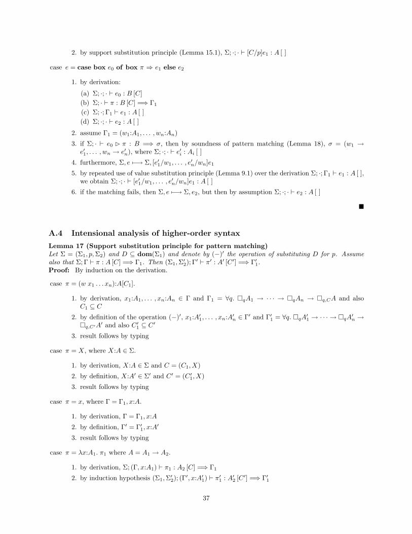
2. by support substitution principle (Lemma 15.1), Σ; ·; · ` [C/p]e1 : A [ ]

case e = case box e0 of box π ⇒ e1 else e2

1. by derivation:

(a) Σ; ·; · ` e0 : B [C](b) Σ; · ` π : B [C] =⇒ Γ1

(c) Σ; ·; Γ1 ` e1 : A [ ](d) Σ; ·; · ` e2 : A [ ]

2. assume Γ1 = (w1:A1, . . . , wn:An)

3. if Σ; · ` e0 � π : B =⇒ σ, then by soundness of pattern matching (Lemma 18), σ = (w1 →e′1, . . . , wn → e′n), where Σ; ·; · ` e′i : Ai [ ]

4. furthermore, Σ, e 7−→ Σ, [e′1/w1, . . . , e′n/wn]e1

5. by repeated use of value substitution principle (Lemma 9.1) over the derivation Σ; ·; Γ1 ` e1 : A [ ],we obtain Σ; ·; · ` [e′1/w1, . . . , e

′n/wn]e1 : A [ ]

6. if the matching fails, then Σ, e 7−→ Σ, e2, but then by assumption Σ; ·; · ` e2 : A [ ]

�

A.4 Intensional analysis of higher-order syntax

Lemma 17 (Support substitution principle for pattern matching)Let Σ = (Σ1, p,Σ2) and D ⊆ dom(Σ1) and denote by (−)′ the operation of substituting D for p. Assumealso that Σ; Γ ` π : A [C] =⇒ Γ1. Then (Σ1,Σ′2); Γ′ ` π′ : A′ [C ′] =⇒ Γ′1.Proof: By induction on the derivation.

case π = (w x1 . . . xn):A[C1].

1. by derivation, x1:A1, . . . , xn:An ∈ Γ and Γ1 = ∀q. �qA1 → · · · → �qAn → �q,CA and alsoC1 ⊆ C

2. by definition of the operation (−)′, x1:A′1, . . . , xn:A′n ∈ Γ′ and Γ′1 = ∀q. �qA′1 → · · · → �qA′n →�q,C′A′ and also C ′1 ⊆ C ′

3. result follows by typing

case π = X, where X:A ∈ Σ.

1. by derivation, X:A ∈ Σ and C = (C1, X)

2. by definition, X:A′ ∈ Σ′ and C ′ = (C ′1, X)

3. result follows by typing

case π = x, where Γ = Γ1, x:A.

1. by derivation, Γ = Γ1, x:A

2. by definition, Γ′ = Γ′1, x:A′

3. result follows by typing

case π = λx:A1. π1 where A = A1 → A2.

1. by derivation, Σ; (Γ, x:A1) ` π1 : A2 [C] =⇒ Γ1

2. by induction hypothesis (Σ1,Σ′2); (Γ′, x:A′1) ` π′1 : A′2 [C ′] =⇒ Γ′1

37

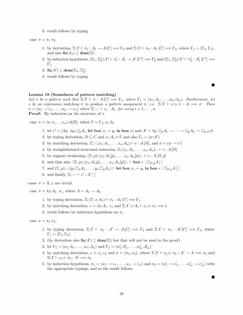
3. result follows by typing

case π = π1 π2.

1. by derivation, Σ; Γ ` π1 : A1 → A [C] =⇒ Γ2 and Σ; Γ ` π2 : A1 [C] =⇒ Γ3, where Γ1 = (Γ2,Γ3),and also fn(A1) ⊆ dom(Σ)

2. by induction hypothesis, (Σ1,Σ′2); Γ′ ` π′1 : A′1 → A′ [C ′] =⇒ Γ′2 and (Σ1,Σ′2); Γ′ ` π′2 : A′1 [C ′] =⇒Γ′3

3. fn(A′) ⊆ dom(Σ1,Σ′2)

4. result follows by typing

�

Lemma 18 (Soundness of pattern matching)Let π be a pattern such that Σ; Γ ` π : A [C] =⇒ Γ1, where Γ1 = (w1:A1, . . . , wn:An). Furthermore, lete be an expression matching π to produce a pattern assignment σ, i.e. Σ; Γ ` e � π : A =⇒ σ. Thenσ = (w1 → e1, . . . , wn → en) where Σ; ·; · ` ei : A1, for every i = 1, . . . , n.Proof: By induction on the structure of π.

case π = (w x1 . . . xn):A[D], where Γ = Γ2, xi:Ai.

1. let e′ = (Λp. λyi:�pAi. let box xi = yi in box e) and A′ = ∀p. �pA1 → · · · → �pAn → �p,DA2. by typing derivation, D ⊆ C and xi:Ai ∈ Γ and also Γ1 = (w:A′)

3. by matching derivation, Σ; ·; (x1:A1, . . . , xn:An) ` e : A [D], and σ = (w → e′)

4. by straightforward structural induction, Σ; (x1:A1, . . . , xn:An); · ` e : A [D]

5. by support weakening, (Σ, p); (x1:A1[p], . . . , xn:An[p]); · ` e : A [D, p]

6. and thus also, (Σ, p); (x1:A1[p], . . . , xn:An[p]); · ` box e : �D,pA [ ]

7. and (Σ, p); ·; (y1:�pA1, . . . , yn:�pAn) ` let box xi = yi in box e : �D,pA [ ]

8. and finally, Σ; ·; · ` e′ : A′ [ ]

cases π = X,x are trivial.

case π = λx:A1. π1, where A = A1 → A2.

1. by typing derivation, Σ; (Γ, x:A1) ` π1 : A2 [C] =⇒ Γ1

2. by matching derivation, e = λx:A1. e1 and Σ; Γ, x:A1 ` e1 � π1 =⇒ σ

3. result follows by induction hypothesis on π1

case π = π2 π3.

1. by typing derivation, Σ; Γ ` π2 : A′ → A [C] =⇒ Γ2 and Σ; Γ ` π3 : A′ [C] =⇒ Γ3, whereΓ1 = (Γ2,Γ3)

2. (by derivation also fn(A′) ⊆ dom(Σ) but that will not be used in the proof)

3. let Γ1 = (w1:A1, . . . , wn:An) and Γ2 = (w′1:A′1, . . . , w′m:A′m)

4. by matching derivation, e = e2 e3 and σ = (σ2, σ3), where Σ; Γ ` e2 � π2 : A′ → A =⇒ σ2 andΣ; Γ ` e3 � π3 : A′ =⇒ σ3

5. by induction hypothesis, σ1 = (w1 → e1, . . . , wn → en) and σ2 = (w′1 → e′1, . . . , w′m → e′m) with

the appropriate typings, and so the result follows

�

38