Embed Size (px)
Citation preview

Meta-Analysis using HLM 6.0
Yaacov Petscher
Florida Center for Reading Research
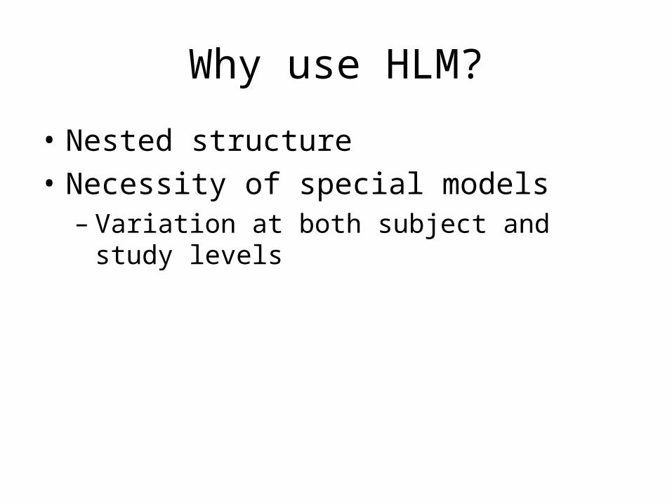
Why use HLM?
• Nested structure
• Necessity of special models– Variation at both subject and study levels
“Special Case” of HLM
• If ES are based on n ≥ 30, we assume approximate normal distribution with sampling variance assumed to be known
• V-known models run in Interactive Mode– Time to brush up on your DOS command
code!
Standardized Mean Difference
• No raw data for us– Must rely on stats to be converted to single
metric
• Many types of statistics that may be usedZ t M/SD
χ² F p-value
r r²
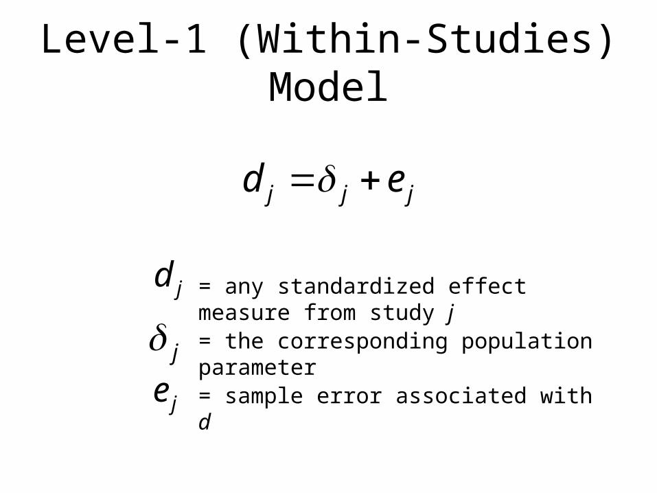
Level-1 (Within-Studies) Model
jjj ed
jd = any standardized effect measure from study j
j = the corresponding population parameter
je = sample error associated with d
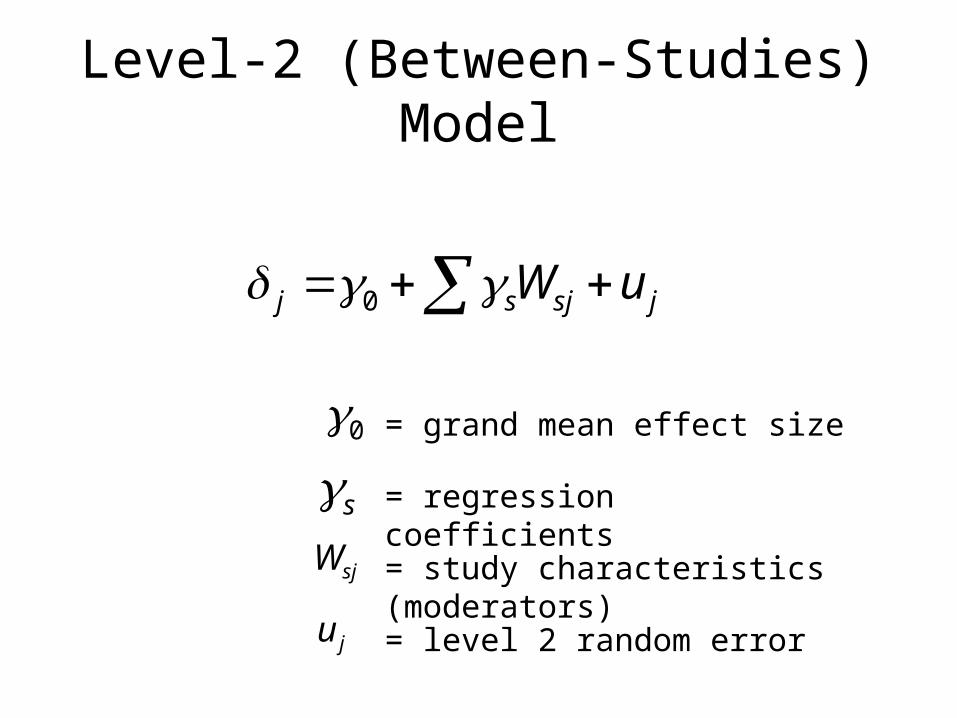
Level-2 (Between-Studies) Model
jsjsj uW 0
0 = grand mean effect size
s = regression coefficients
sjW = study characteristics (moderators)
ju = level 2 random error

Combined Model
s
jjssj euWd 0
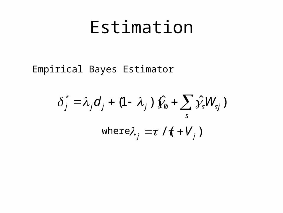
Estimation
s
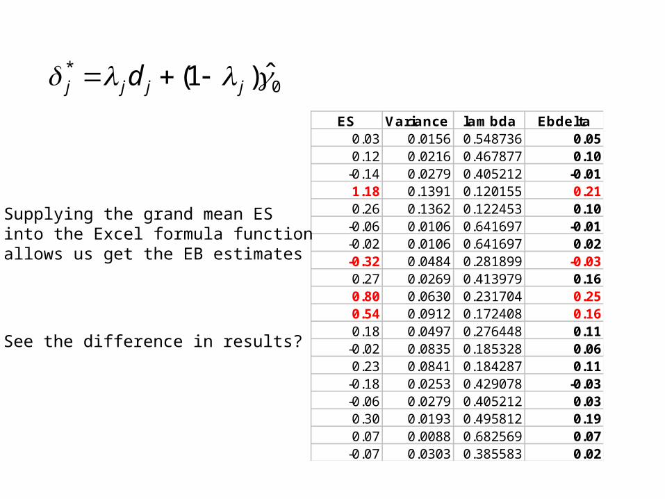
sjsjjjj Wd )ˆˆ)(1( 0*
Empirical Bayes Estimator
)/( jj V where
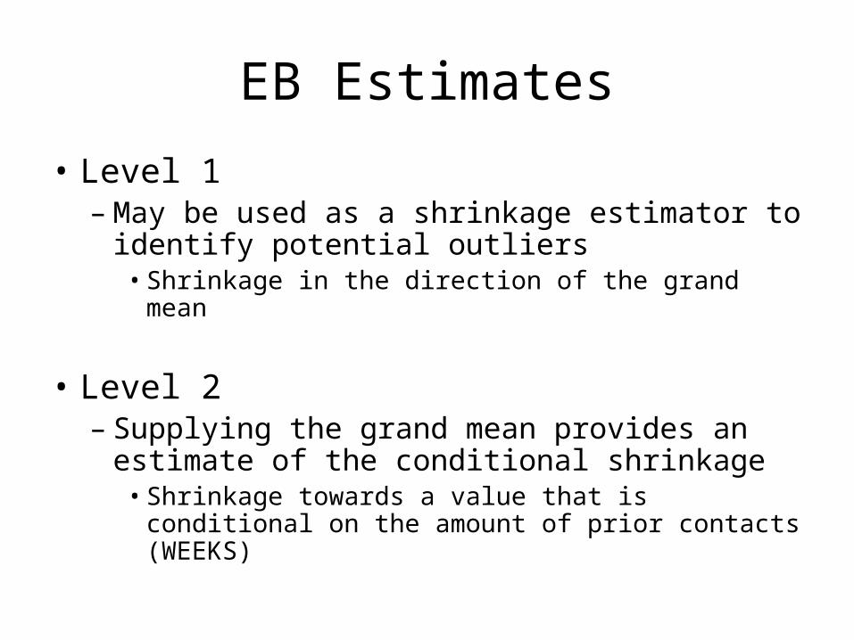
EB Estimates
• Level 1– May be used as a shrinkage estimator to
identify potential outliers • Shrinkage in the direction of the grand mean
• Level 2– Supplying the grand mean provides an
estimate of the conditional shrinkage • Shrinkage towards a value that is conditional on
the amount of prior contacts (WEEKS)
The following example will be run using data from Raudenbush & Bryk
Chapter 7 data (pg 211)
The Effect of Teacher Expectancy on Pupil IQ
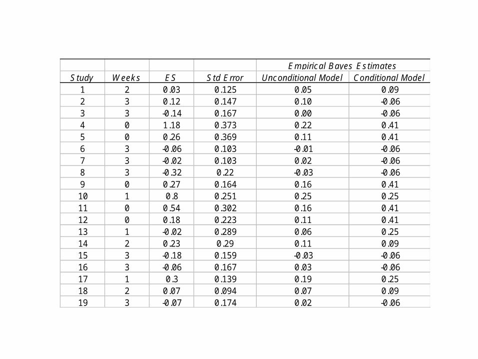
Study Week s ES Std Error Unconditional Model Conditional Model1 2 0.03 0.125 0.05 0.092 3 0.12 0.147 0.10 -0.063 3 -0.14 0.167 0.00 -0.064 0 1.18 0.373 0.22 0.415 0 0.26 0.369 0.11 0.416 3 -0.06 0.103 -0.01 -0.067 3 -0.02 0.103 0.02 -0.068 3 -0.32 0.22 -0.03 -0.069 0 0.27 0.164 0.16 0.4110 1 0.8 0.251 0.25 0.2511 0 0.54 0.302 0.16 0.4112 0 0.18 0.223 0.11 0.4113 1 -0.02 0.289 0.06 0.2514 2 0.23 0.29 0.11 0.0915 3 -0.18 0.159 -0.03 -0.0616 3 -0.06 0.167 0.03 -0.0617 1 0.3 0.139 0.19 0.2518 2 0.07 0.094 0.07 0.0919 3 -0.07 0.174 0.02 -0.06
Empirical Bayes Estimates
Some Calculations
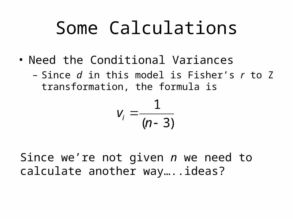
• Need the Conditional Variances– Since d in this model is Fisher’s r to Z transformation,
the formula is
)3(
1
n
vi
Since we’re not given n we need to calculate another way…..ideas?
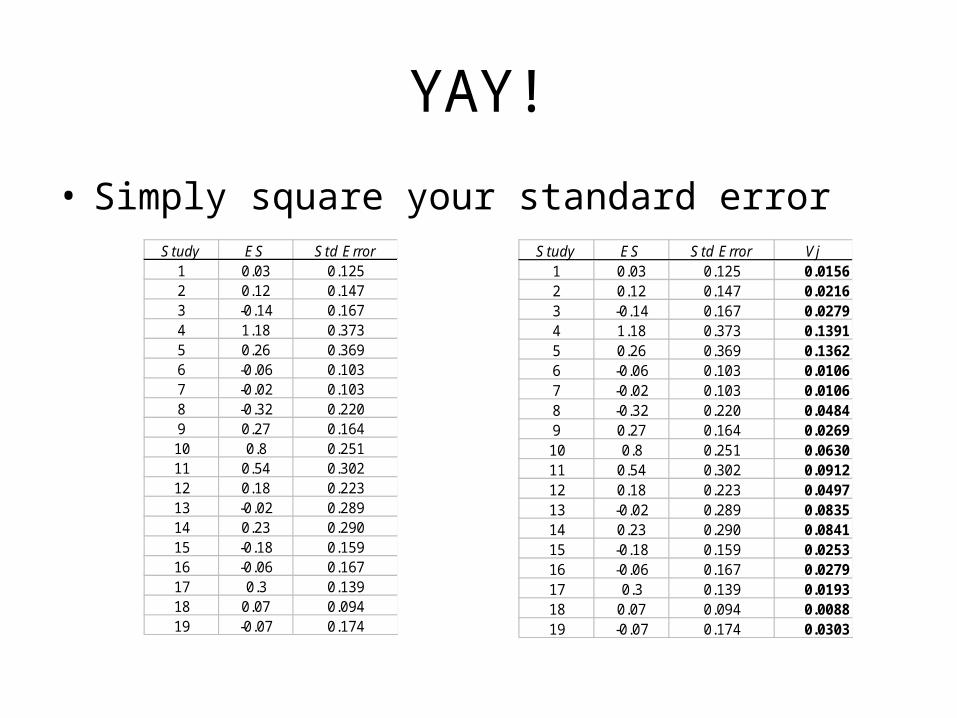
YAY!
• Simply square your standard errorStudy ES Std Error
1 0.03 0.1252 0.12 0.1473 -0.14 0.1674 1.18 0.3735 0.26 0.3696 -0.06 0.1037 -0.02 0.1038 -0.32 0.2209 0.27 0.16410 0.8 0.25111 0.54 0.30212 0.18 0.22313 -0.02 0.28914 0.23 0.29015 -0.18 0.15916 -0.06 0.16717 0.3 0.13918 0.07 0.09419 -0.07 0.174
Study ES Std Error Vj1 0.03 0.125 0.01562 0.12 0.147 0.02163 -0.14 0.167 0.02794 1.18 0.373 0.13915 0.26 0.369 0.13626 -0.06 0.103 0.01067 -0.02 0.103 0.01068 -0.32 0.220 0.04849 0.27 0.164 0.026910 0.8 0.251 0.063011 0.54 0.302 0.091212 0.18 0.223 0.049713 -0.02 0.289 0.083514 0.23 0.290 0.084115 -0.18 0.159 0.025316 -0.06 0.167 0.027917 0.3 0.139 0.019318 0.07 0.094 0.008819 -0.07 0.174 0.0303
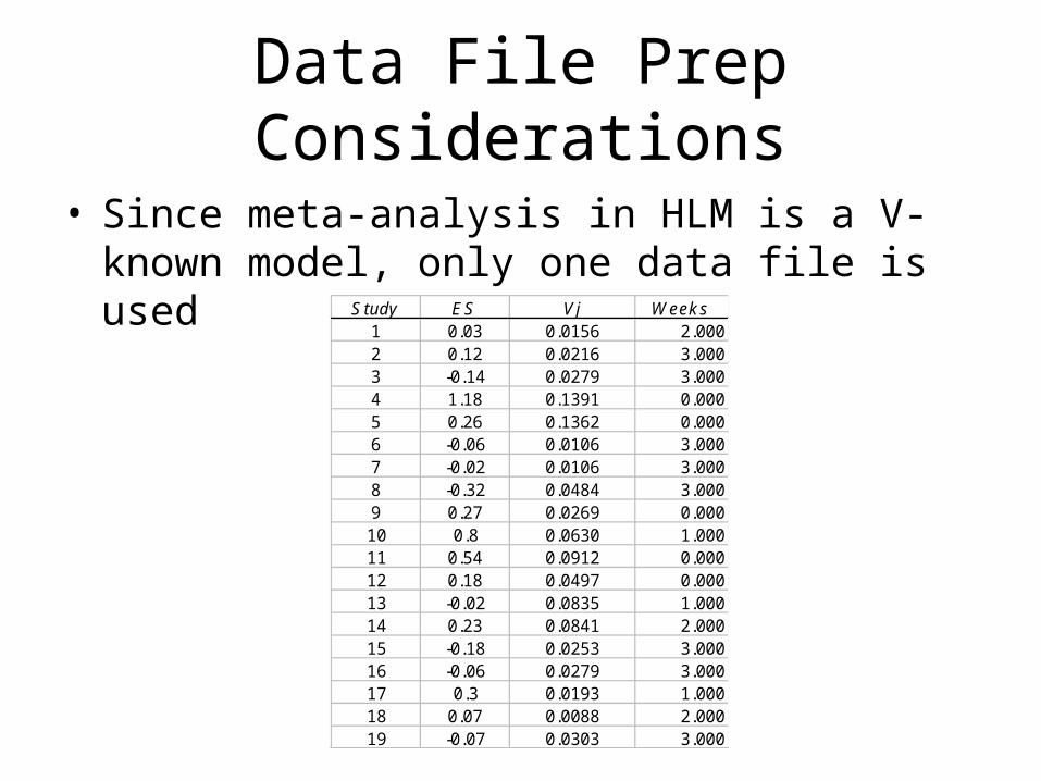
Data File Prep Considerations
• Since meta-analysis in HLM is a V-known model, only one data file is used
Study ES Vj Week s1 0.03 0.0156 2.0002 0.12 0.0216 3.0003 -0.14 0.0279 3.0004 1.18 0.1391 0.0005 0.26 0.1362 0.0006 -0.06 0.0106 3.0007 -0.02 0.0106 3.0008 -0.32 0.0484 3.0009 0.27 0.0269 0.00010 0.8 0.0630 1.00011 0.54 0.0912 0.00012 0.18 0.0497 0.00013 -0.02 0.0835 1.00014 0.23 0.0841 2.00015 -0.18 0.0253 3.00016 -0.06 0.0279 3.00017 0.3 0.0193 1.00018 0.07 0.0088 2.00019 -0.07 0.0303 3.000
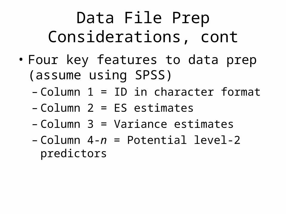
Data File Prep Considerations, cont
• Four key features to data prep (assume using SPSS)– Column 1 = ID in character format– Column 2 = ES estimates – Column 3 = Variance estimates– Column 4-n = Potential level-2 predictors
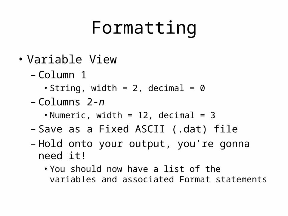
Formatting
• Variable View– Column 1
• String, width = 2, decimal = 0
– Columns 2-n• Numeric, width = 12, decimal = 3
– Save as a Fixed ASCII (.dat) file– Hold onto your output, you’re gonna need it!
• You should now have a list of the variables and associated Format statements
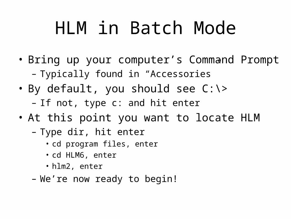
HLM in Batch Mode
• Bring up your computer’s Command Prompt– Typically found in “Accessories”
• By default, you should see C:\>– If not, type c: and hit enter
• At this point you want to locate HLM– Type dir, hit enter
• cd program files, enter• cd HLM6, enter• hlm2, enter
– We’re now ready to begin!
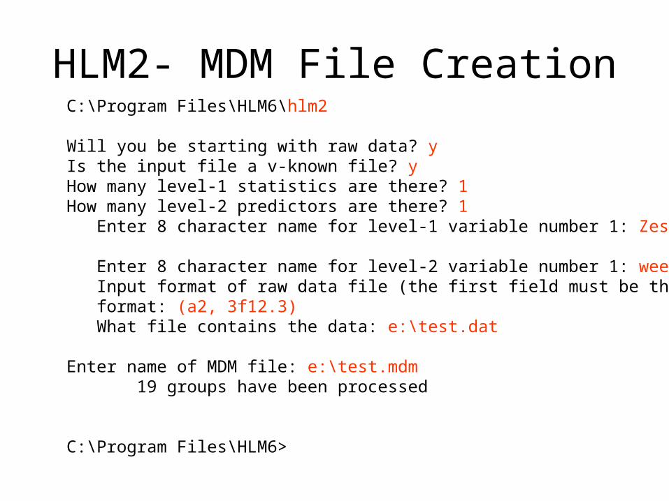
HLM2- MDM File CreationC:\Program Files\HLM6\hlm2
Will you be starting with raw data? yIs the input file a v-known file? yHow many level-1 statistics are there? 1How many level-2 predictors are there? 1 Enter 8 character name for level-1 variable number 1: Zes
Enter 8 character name for level-2 variable number 1: weeks Input format of raw data file (the first field must be the character ID) format: (a2, 3f12.3) What file contains the data: e:\test.dat
Enter name of MDM file: e:\test.mdm 19 groups have been processed
C:\Program Files\HLM6>
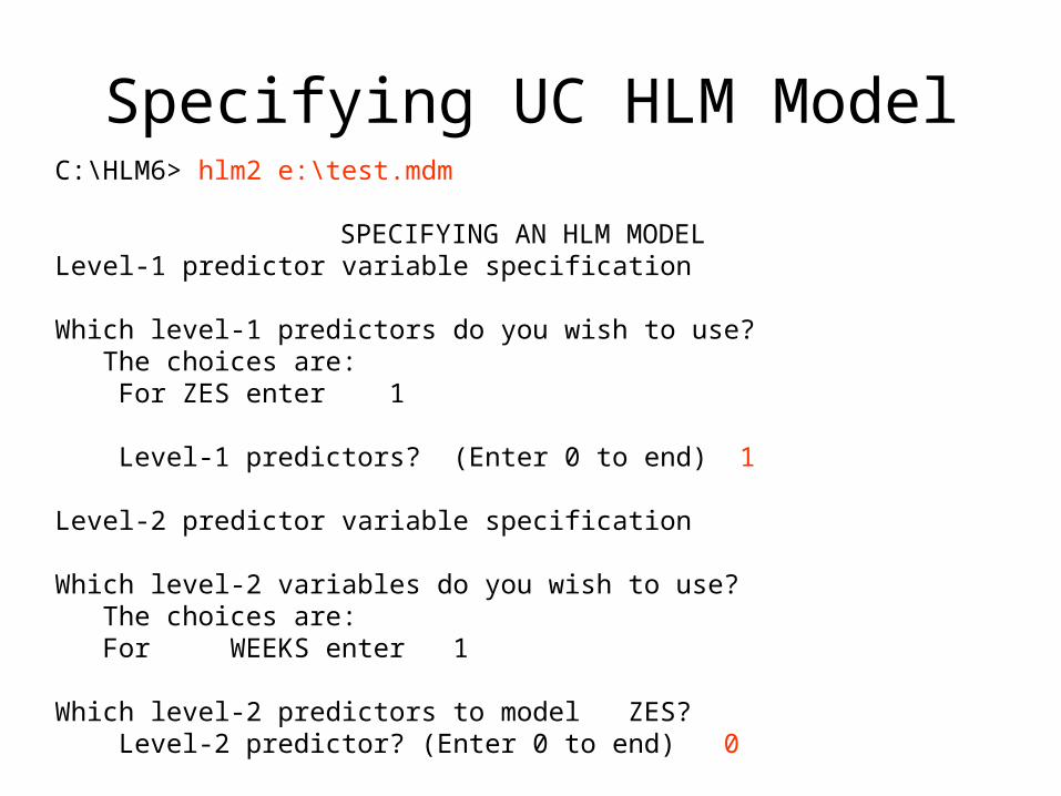
Specifying UC HLM ModelC:\HLM6> hlm2 e:\test.mdm
SPECIFYING AN HLM MODEL Level-1 predictor variable specification
Which level-1 predictors do you wish to use? The choices are: For ZES enter 1
Level-1 predictors? (Enter 0 to end) 1
Level-2 predictor variable specification
Which level-2 variables do you wish to use? The choices are: For WEEKS enter 1
Which level-2 predictors to model ZES? Level-2 predictor? (Enter 0 to end) 0
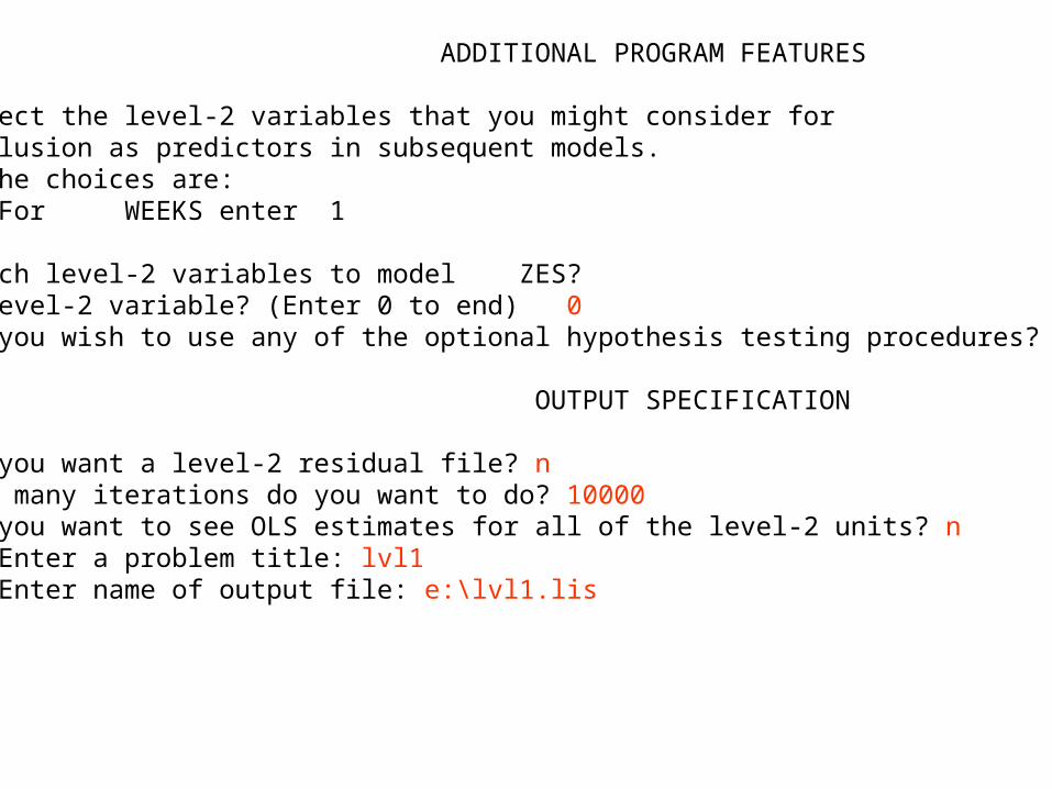
ADDITIONAL PROGRAM FEATURES
Select the level-2 variables that you might consider for Inclusion as predictors in subsequent models. The choices are: For WEEKS enter 1
Which level-2 variables to model ZES? Level-2 variable? (Enter 0 to end) 0Do you wish to use any of the optional hypothesis testing procedures? n
OUTPUT SPECIFICATION
Do you want a level-2 residual file? nHow many iterations do you want to do? 10000Do you want to see OLS estimates for all of the level-2 units? n Enter a problem title: lvl1 Enter name of output file: e:\lvl1.lis
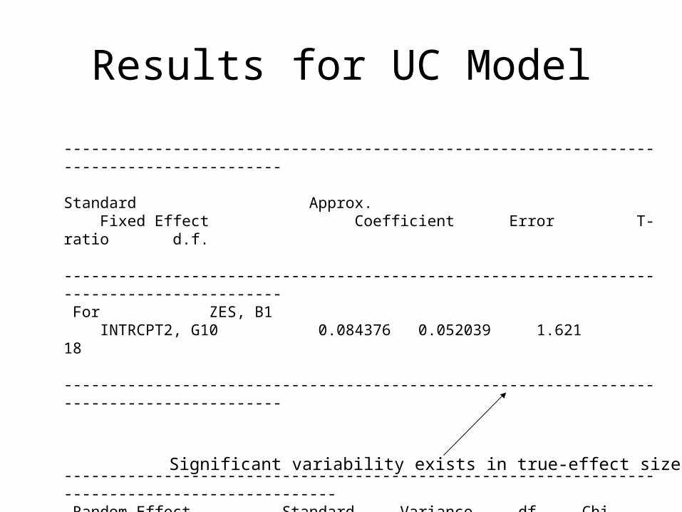
Results for UC Model ----------------------------------------------------------------------------------------- Standard Approx. Fixed Effect Coefficient Error T-ratio d.f. ----------------------------------------------------------------------------------------- For ZES, B1 INTRCPT2, G10 0.084376 0.052039 1.621 18 -----------------------------------------------------------------------------------------
----------------------------------------------------------------------------------------------- Random Effect Standard Variance df Chi-square P-value Deviation Component ------------------------------------------------------------------------------------------------ ZES, U1 0.13896 0.01931 18 36.25115 0.007 ------------------------------------------------------------------------------------------------
Significant variability exists in true-effect sizes
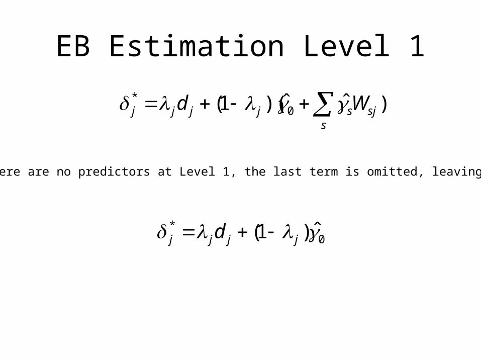
EB Estimation Level 1
s
sjsjjjj Wd )ˆˆ)(1( 0*
Since there are no predictors at Level 1, the last term is omitted, leaving us with
0* ˆ)1( jjjj d
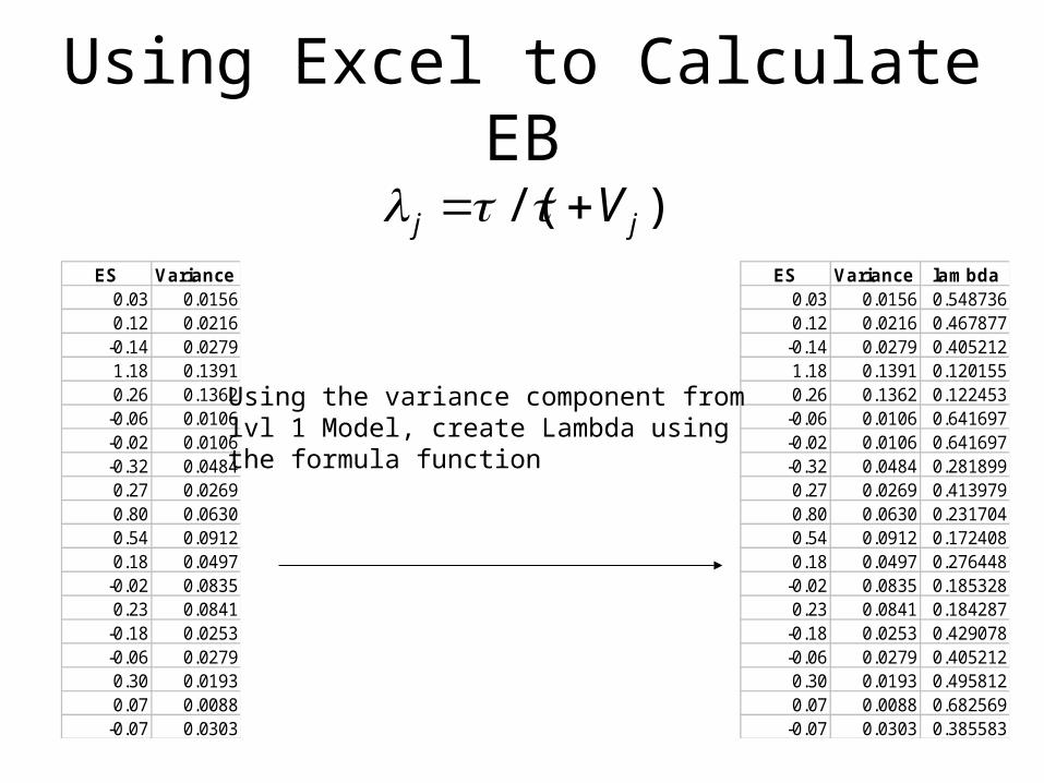
Using Excel to Calculate EB
)/( jj V ES Variance
0.03 0.01560.12 0.0216
-0.14 0.02791.18 0.13910.26 0.1362
-0.06 0.0106-0.02 0.0106-0.32 0.04840.27 0.02690.80 0.06300.54 0.09120.18 0.0497
-0.02 0.08350.23 0.0841
-0.18 0.0253-0.06 0.02790.30 0.01930.07 0.0088
-0.07 0.0303
ES Variance lambda0.03 0.0156 0.5487360.12 0.0216 0.467877
-0.14 0.0279 0.4052121.18 0.1391 0.1201550.26 0.1362 0.122453
-0.06 0.0106 0.641697-0.02 0.0106 0.641697-0.32 0.0484 0.2818990.27 0.0269 0.4139790.80 0.0630 0.2317040.54 0.0912 0.1724080.18 0.0497 0.276448
-0.02 0.0835 0.1853280.23 0.0841 0.184287
-0.18 0.0253 0.429078-0.06 0.0279 0.4052120.30 0.0193 0.4958120.07 0.0088 0.682569
-0.07 0.0303 0.385583
Using the variance component fromlvl 1 Model, create Lambda usingthe formula function
0* ˆ)1( jjjj d
ES Variance lambda Ebdelta0.03 0.0156 0.548736 0.050.12 0.0216 0.467877 0.10
-0.14 0.0279 0.405212 -0.011.18 0.1391 0.120155 0.210.26 0.1362 0.122453 0.10
-0.06 0.0106 0.641697 -0.01-0.02 0.0106 0.641697 0.02-0.32 0.0484 0.281899 -0.030.27 0.0269 0.413979 0.160.80 0.0630 0.231704 0.250.54 0.0912 0.172408 0.160.18 0.0497 0.276448 0.11
-0.02 0.0835 0.185328 0.060.23 0.0841 0.184287 0.11
-0.18 0.0253 0.429078 -0.03-0.06 0.0279 0.405212 0.030.30 0.0193 0.495812 0.190.07 0.0088 0.682569 0.07
-0.07 0.0303 0.385583 0.02
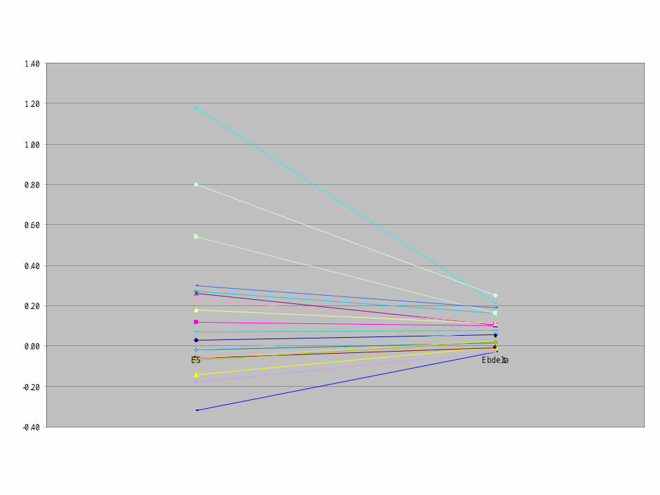
Supplying the grand mean ESinto the Excel formula function allows us get the EB estimates
See the difference in results?
-0.40
-0.20
0.00
0.20
0.40
0.60
0.80
1.00
1.20
1.40
ES Ebdelta
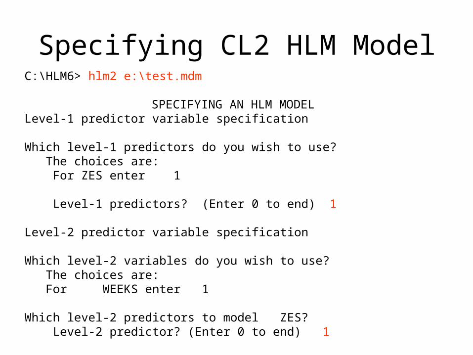
Specifying CL2 HLM ModelC:\HLM6> hlm2 e:\test.mdm
SPECIFYING AN HLM MODEL Level-1 predictor variable specification
Which level-1 predictors do you wish to use? The choices are: For ZES enter 1
Level-1 predictors? (Enter 0 to end) 1
Level-2 predictor variable specification
Which level-2 variables do you wish to use? The choices are: For WEEKS enter 1
Which level-2 predictors to model ZES? Level-2 predictor? (Enter 0 to end) 1
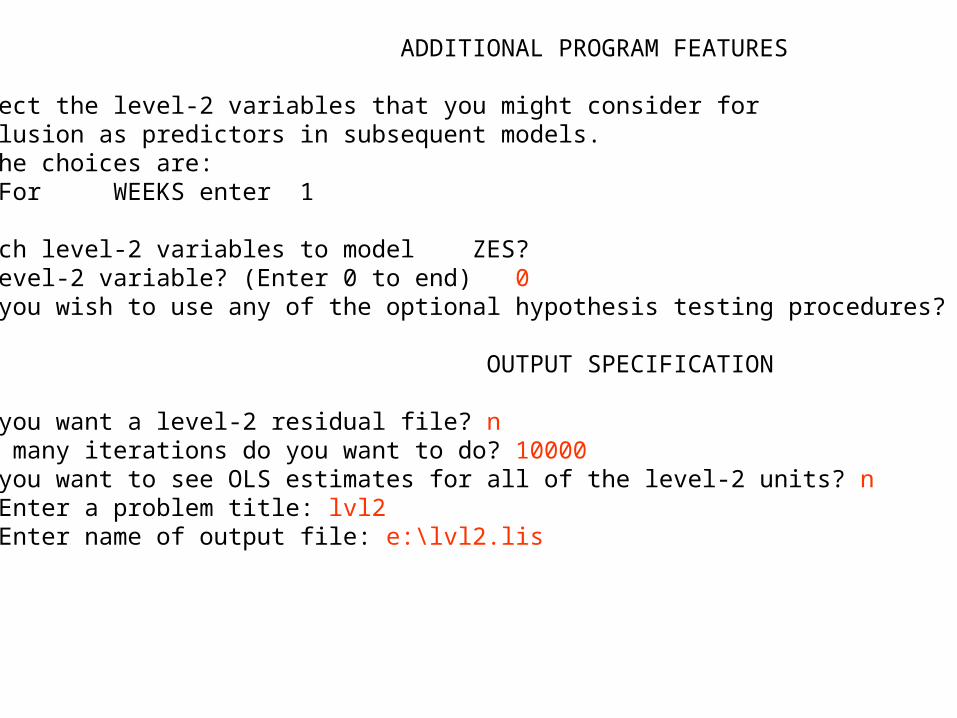
ADDITIONAL PROGRAM FEATURES
Select the level-2 variables that you might consider for Inclusion as predictors in subsequent models. The choices are: For WEEKS enter 1
Which level-2 variables to model ZES? Level-2 variable? (Enter 0 to end) 0Do you wish to use any of the optional hypothesis testing procedures? n
OUTPUT SPECIFICATION
Do you want a level-2 residual file? nHow many iterations do you want to do? 10000Do you want to see OLS estimates for all of the level-2 units? n Enter a problem title: lvl2 Enter name of output file: e:\lvl2.lis
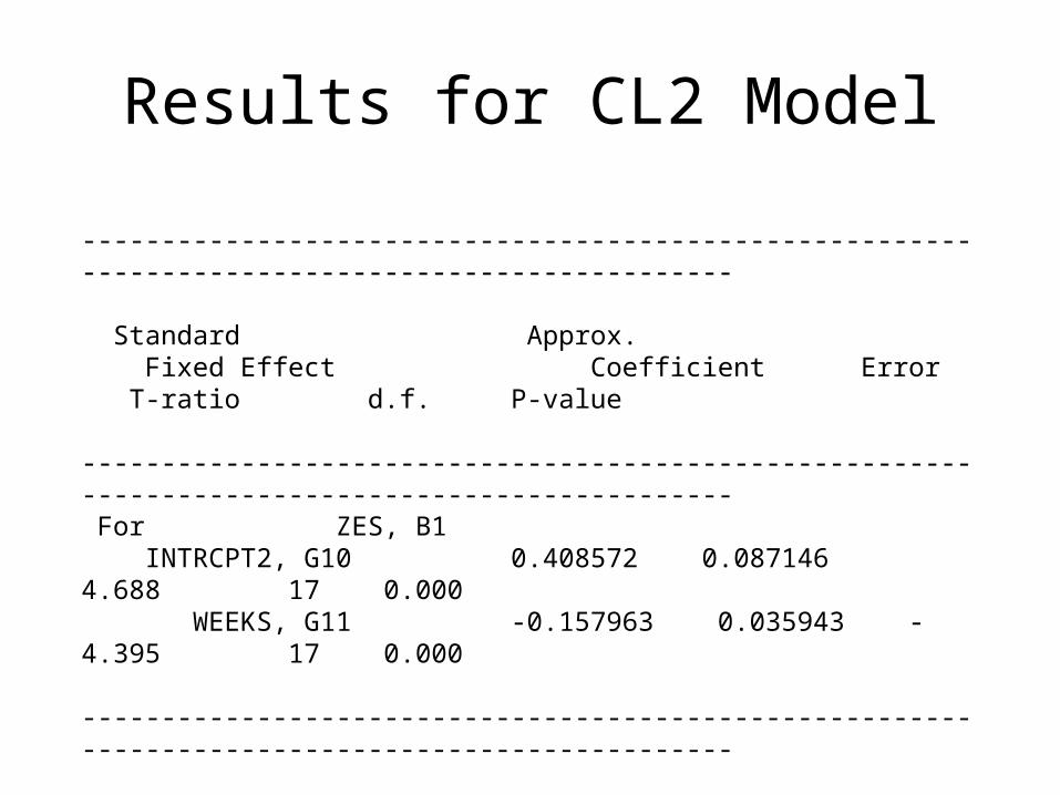
Results for CL2 Model
------------------------------------------------------------------------------------------------- Standard Approx. Fixed Effect Coefficient Error T-ratio d.f. P-value ------------------------------------------------------------------------------------------------- For ZES, B1 INTRCPT2, G10 0.408572 0.087146 4.688 17 0.000 WEEKS, G11 -0.157963 0.035943 -4.395 17 0.000 -------------------------------------------------------------------------------------------------
------------------------------------------------------------------------------------------------ Random Effect Standard Variance df Chi-square P-value Deviation Component ------------------------------------------------------------------------------------------------ ZES, U1 0.00283 0.00001 17 16.53614 >.500 ------------------------------------------------------------------------------------------------

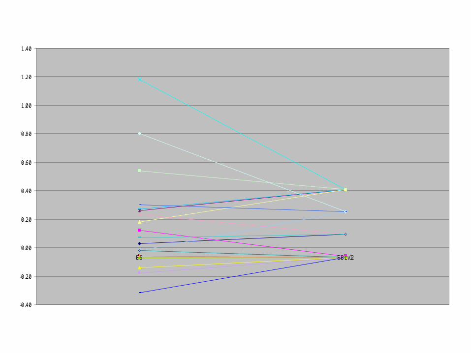
EB Estimation Level 2
Since then = 0 and we’re left with 0ˆ )/( jj V
jj WEEKS)(ˆˆ 10*
ES Weeks EBLvl20.03 2 0.090.12 3 -0.06
-0.14 3 -0.071.18 0 0.410.26 0 0.41
-0.06 3 -0.07-0.02 3 -0.07-0.32 3 -0.070.27 0 0.410.80 1 0.250.54 0 0.410.18 0 0.41-0.02 1 0.250.23 2 0.09
-0.18 3 -0.07-0.06 3 -0.070.30 1 0.250.07 2 0.09
-0.07 3 -0.07
Using G10 and G11, we can calculatethe EB estimates for Level 2
-0.40
-0.20
0.00
0.20
0.40
0.60
0.80
1.00
1.20
1.40
ES EBLvl2
EB Estimation Level 2
• Since our Level-2 predictor takes on one of four different values, the shrinkage is towards one of the four points.

End(for now)